subsea compression gullfaks sør satellite field -...
TRANSCRIPT

FAKULTET FOR INGENIØRVITENSKAP OG TEKNOLOGI, NTNU
Subsea compression Gullfaks
Sør satellite field EiT - Gullfaks village 2013
Group 1
Teyyub Amirbayov, Juan Carlos Gloria Lopez, Dicky Harishidayat, Ailo Aasen, Ole Christian Auran
and Malin Kristina Salmi Stavrum
05/02/2013

1
Abstract
To achieve a higher gas recovery from the Gullfaks Sør field, Statoil has planned to implement subsea
compression in the Gullfaks Sør field in October 2015. The project focus was to find a simple way to
model this, and to evaluate the effect of the subsea compressor on the net present value (NPV). We
considered two subsea production templates (L- and M-template), both during pre-compression and
after installation. We try to determine the value of the compressor by comparing the NPVs in different
scenarios, with and without subsea compression. In addition to subsea compression, we have evaluated
different strategies of enhancing production, like optimizing the production strategy and doing low-
pressure separation. In addition, we have tried to model the compressor and validate its characteristics,
and also done some flow assurance related to hydrate formation.

2
Preface This report is written as part of TPG 4851 Experts in Team, Gullfaks Village spring 2013, in
cooperation with the Statoil Gullfaks license in Bergen. The goal of this village has been to review
new ways to increase the gas recovery from the satellite field, Gullfaks Sør by installing new subsea
equipment or other modifications.
We would like to thank the village supervisors Professor Michael Golan, Professor Jon Kleppe, PhD
students Milan Edvard Wolf Stanko, Mayembe Joao Bartolome and Jesus Alberto De Andrade
Correia, and associate professor Jan Ivar Jensen for helpful guidance throughout the project.
We would also like to thank the project supervisor Hallstein M. Ånesand and Petter Eltvik in Statoil.
Trondheim, May 2013
Teyyub Amirbayov, Ailo Aasen
Juan Carlos Glora Lopez
Ole Christian Auran
Dicky Harishidayat
Malin Kristina Salmi Stavrum

3
Table of Contents
Abstract........................................................................................................................................ 1
Preface ......................................................................................................................................... 2
1. Introduction........................................................................................................................... 4
2. Part A ................................................................................................................................... 7
2.1 Method of execution ....................................................................................................... 7
2.2 Results and discussion .................................................................................................... 8
2.2.1 Compressor map ....................................................................................................11
3. Part B...................................................................................................................................12
3.1 Material balance calculations based on black oil properties ....................................................12
3.1.1 Results from IPT- Material balance................................................................................16
3.2 Wet gas compression ..........................................................................................................19
3.2.1 Compressor validation ..................................................................................................19
3.2.2 Wet gas compressors in parallel .....................................................................................21
3.2.3 Wet gas compressors in series .......................................................................................21
3.3 Flow assurance, hydrate formation .......................................................................................22
3.3.1 14” Pipeline ...........................................................................................................24
3.3.2 8” pipeline .............................................................................................................24
3.4 Production management in different scenarios ......................................................................25
3.4.1 Modifying the Excel model from part A .........................................................................26
3.4.2 Scenario 1B: Shutting down one of the pipes in 2015 ......................................................27
3.4.1 Scenario 2B: The best case - finding an optimal production strategy ................................27
4. Economical calculations ...........................................................................................................31
4.1 General economy ................................................................................................................31
4.2 Evaluating the NPV of the compressor project in different scenarios ......................................33
4.2 Evaluating the production management scenarios..................................................................35
5. Summary and recommendations ................................................................................................37
List of Symbols, abbrevation and Quantities used...........................................................................38
Literature.....................................................................................................................................39
List of appendix ...........................................................................................................................40

4
1. Introduction
The Gullfaks field started producing oil and gas December 1986. After the discovery in 1978, the field
was assigned to three Norwegian companies: Statoil, Norsk Hydro and Saga Petroleum, with Statoil as
the operator. Since production-start, Statoil has used new technologies, such as horizontal and long-
ranged wells and alternating water and gas injections to achieve a high recovery for oil and gas from
the field. The recovery factor of Gullfaks today is estimated to be 59 %, but the goal is increasing it to
62%. Increasing the oil and gas recovery is the key concept for the Gullfaks Village.
The Gullfaks field lies in block 34/10 of the northern part of the North Sea. The main field has three
production platforms (A, B and C) with concrete substructure. The satellite fields Gullfaks Sør,
Rimfaks, Skinfaks og Gullveig has been developed with subsea wells which are remotely operated
from Gullfaks A and C platforms. The Gullfaks field is illustrated in figure 1. [1]
Figure 1 Map of Gullfaks area. The subsea satellite Gullfaks Sør field is shown in the blue circle, to the south of the
Gullfaks main field. [2]
The object for this project was to boost and sustain gas and condensate production from the Gullfaks
Sør subsea satellite field for template L and M. The L and M templates are illustrated in the Gullfaks

5
field layout in figure 2. Gullfaks Sør lies in the blocks 34/10 and 33/12, and the water depth of the
satellite area is in the range from 130- to 220 meter. Gas from the L- and M field is transported by
2*14” pipeline of 14 km length to Gullfaks C. On the platform the gas is treated and then further
transported by pipeline to Kårstø, Stavanger. The gas produced from the Gullfaks Sør field contains
condensate which makes the gas more valuable. [3]
Figure 2 Layout for the satellites fields Gullfaks Sør, Gullveig, Rimfaks and Skinnfaks. [4]
To achieve a higher gas recovery factor from the Gullfaks Sør field, Statoil is installing a multi-phase
subsea compressor which is planned to start in 2015. The technology of a multi-phase compressor
makes it possible for increased boosting of gas containing condensate and water, which earlier had to
be removed upstream in conventional compressors. [5]
Statoil has estimated that the reservoir pressure in the Gullfaks Sør field is reduced to its limit to
obtain the 10 MSm3/day plateau in 2015, and therefore the compression is essential to keep the plateau
production. The wet gas compression combined with low-pressure modification (LPM) in a later phase
can increase the recovery factor from the Gullfaks field from 62% to 74%. Low-pressure modification
means reducing the separator pressure of the first stage separator at the platform. [6]
The implementation of the wet gas compressor is estimated to give an extra 22 million barrels and 3
billion standard cubic meter gas from the Gullfaks Sør Brent reservoir. Statoil has invested
approximately 3 billion NOK in the wet gas compressor project at the Gullfaks Sør field. [6]

6
A sketch of the L- and M template with the multi-phase compressor system is illustrated in figure 3.
The M- template is only operating three wells and not four as shown in figure 3.
The project was divided in two tasks, A and B. In part A, a simple dry gas model was made in excel to
try to extend the natural plateau of 10 MSm3/day as long as possible.
In part B several cases were studied. First of all a material balance excel sheet provided made by PhD
Milan Stanko was used to see if the assumptions used in part A could be used for the wet gas model.
The compressor arrangement was studied to see if the compressors were to run in parallel or in series,
and at what time this should happen. A simple wet gas compressor model was made in HYSYS, low
pressure modification was used to prolong the plateau. Since the overall goal of the Gullfaks village is
to increase the recovery factor and value of the Gullfaks field, this motivates the flow optimization we
have done, where we utilize all the value-enhancing technology (e.g. the compressor) at our disposal,
and come up with an optimal production strategy. This was time-consuming work, but fortunately it
has a conclusion that is easy to understand.
Figure 3 Template L and M. Sketch courtesy of technical supervisor Michael Golan. [7]

7
2. Part A
In part A, a model was established in Excel, using the following main assumptions:
Dry gas only
Isothermal equations valid
Only horizontal flow from templates to platform, neglecting vertical pressure loss in
riser
Project start: January 1st 2009
Project ends when production goes below 5 MSm3/day
Used two 14” pipes after towhead, 8” not used
No low-pressure modification
All 7 wells are identical
Wells in the same template have the same wellhead pressure
Also a simulation was run; we will refer to this as Scenario A. The economic analysis is done in part
B, section 4.
2.1 Method of execution
After being presented the relevant data for template L and M (appendix 1) and a simplified set of
governing equations (1-4), an excel model was made. The excel sheet made in part A is presented in
appendix 2.
Material balance to calculate reservoir pressure:
(
) (
) (1)
Pressure in horizontal pipeline:
(
)
(2)
Tubing equation:
(
)
(3)
Inflow equation reservoir to wellfloor
(
) (4)
where pR is reservoir pressure, pi the initial pressure, zR, zi are compressibility factors, G is the gas
initially in place, is the gas produced, CFL is the pre-compression spool coefficient, CT is the Tubing
coefficient, CR the Reservoir coefficient, pwf is the wellfloor pressure.
8
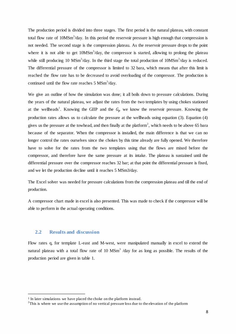
The production period is divided into three stages. The first period is the natural plateau, with constant
total flow rate of 10MSm3/day. In this period the reservoir pressure is high enough that compression is
not needed. The second stage is the compression plateau. As the reservoir pressure drops to the point
where it is not able to get 10MSm3/day, the compressor is started, allowing to prolong the plateau
while still producing 10 MSm3/day. In the third stage the total production of 10MSm
3/day is reduced.
The differential pressure of the compressor is limited to 32 bara, which means that after this limit is
reached the flow rate has to be decreased to avoid overloading of the compressor. The production is
continued until the flow rate reaches 5 MSm3/day.
We give an outline of how the simulation was done; it all boils down to pressure calculations. During
the years of the natural plateau, we adjust the rates from the two templates by using chokes stationed
at the wellheads1. Knowing the GIIP and the we know the reservoir pressure. Knowing the
production rates allows us to calculate the pressure at the wellheads using equation (3). Equation (4)
gives us the pressure at the towhead, and then finally at the platform2, which needs to be above 65 bara
because of the separator. When the compressor is installed, the main difference is that we can no
longer control the rates ourselves since the chokes by this time already are fully opened. We therefore
have to solve for the rates from the two templates using that the flows are mixed before the
compressor, and therefore have the same pressure at its intake. The plateau is sustained until the
differential pressure over the compressor reaches 32 bar; at that point the differential pressure is fixed,
and we let the production decline until it reaches 5 MSm3/day.
The Excel solver was needed for pressure calculations from the compression plateau and till the end of
production.
A compressor chart made in excel is also presented. This was made to check if the compressor will be
able to perform in the actual operating conditions.
2.2 Results and discussion
Flow rates q, for template L-east and M-west, were manipulated manually in excel to extend the
natural plateau with a total flow rate of 10 MSm3 /day for as long as possible. The results of the
production period are given in table 1.
1 In later simulations we have placed the choke on the platform instead. 2This is where we use the assumption of no vertical pressure loss due to the elevation of the platform

9
Table 1 Results of the end of natural-, compression plateau and production.
End of: Year
Natural plateau June 2016
Compression plateau July 2018
Production January 2025
Figure 4 illustrates the flow rate for template L and M during the production period from 2009 to
2025. Figure 5 and 6 illustrates the pressures for the well-head, well flow, reservoir, separator,
towhead and template during the production period for template L and M respectively. In these figures
the choke is the difference betwen pwh and Ptemplate. The graph for Ptemplate lies underneath Ptowhead , since
the pressure loss from the template to the towhead is negligible.
Figure 4 Flow rate of template L and M versus time in production period
Figure 5 Well head-, well flow-, reservoir-, separator-, towhead- and template pressure for template-L versus time.
000,0E+0
1,0E+6
2,0E+6
3,0E+6
4,0E+6
5,0E+6
6,0E+6
7,0E+6
8,0E+6
9,0E+6
Flo
w r
ate
q (
Sm3
/da
y)
Year
Template L,East
Template M,West
-50
0
50
100
150
200
250
300
Pre
ssu
re (b
ara
)
Year
Template L
P Well head
P well flow
P reservoar
P seperator
P towhead
P template

10
Figure 6 Well head-, well flow-, reservoir-, separator-, towhead- and template pressure for template M versus time.
The total decreasing production flow rate is illustrated in figure 7.
Figure 7 The total flow rate for template M and L in between year 2008 - 2024.
As can be seen in Figure 4, during the natural plateau we increased the production from L and
decreased production from M. This is related to the fact that the GIIP for the two reservoirs differ by a
factor of 3.
In figure 5 and 6, we give an overview of how the pressures at some stages in the transport of the gas
from the reservoir on its way to the platform.
-50
0
50
100
150
200
250P
ress
ure
(ba
ra)
Year
Template M
P well head
P well flow
P reservoar
P seperator
P Towhead
P template
000,0E+0
2,0E+6
4,0E+6
6,0E+6
8,0E+6
10,0E+6
12,0E+6
Tota
l flo
w r
ate
, q (
Sm3
/day
)
Year
Flow rate, q total

11
The recovery factors for field L and M at the end of production, can be viewed in figure 8, and were
determined to be 0.61 and 0.71 respectively.
2.2.1 Compressor map
After running tests on the compressor, Framo Engineering claims the compressor has no operational
constrains related to Surge (minimum flow rate), stone wall (maximum flow rate), or mechanical
issues. No information have been given on minimal suction pressure of the compressor, this is
therefore not included as a constraint. Constraints related to the compressor are as follows:
Compressor speed: N= (2000-4500) rpm. A recommendation from Framo Engineering.
Discharge temperature: Td < 110°C. This limitation is related to buckling of the pipe.
Minimum inlet temperature is set to 35°C.
Power consumption of each compressor is set to a maximum of 5MW.
Maximum pressure increase over one compressor (ΔP) is 32 bar.
Maximum pressure increase over both compressors is 60 bar
Maximum flow capacity of each compressor is 6000 m3/h.
Results from the compressor map is based on the flow rates and pressures from the excel file
(appendix 1). One compressor map was made for each year. For each year the compressors were set in
parallel and in series. Variables changing during the test were suction pressure, discharge pressure and
inlet flow. The inlet temperature was fixed at 35°C. The compressor maps are illustrated in appendix
3.
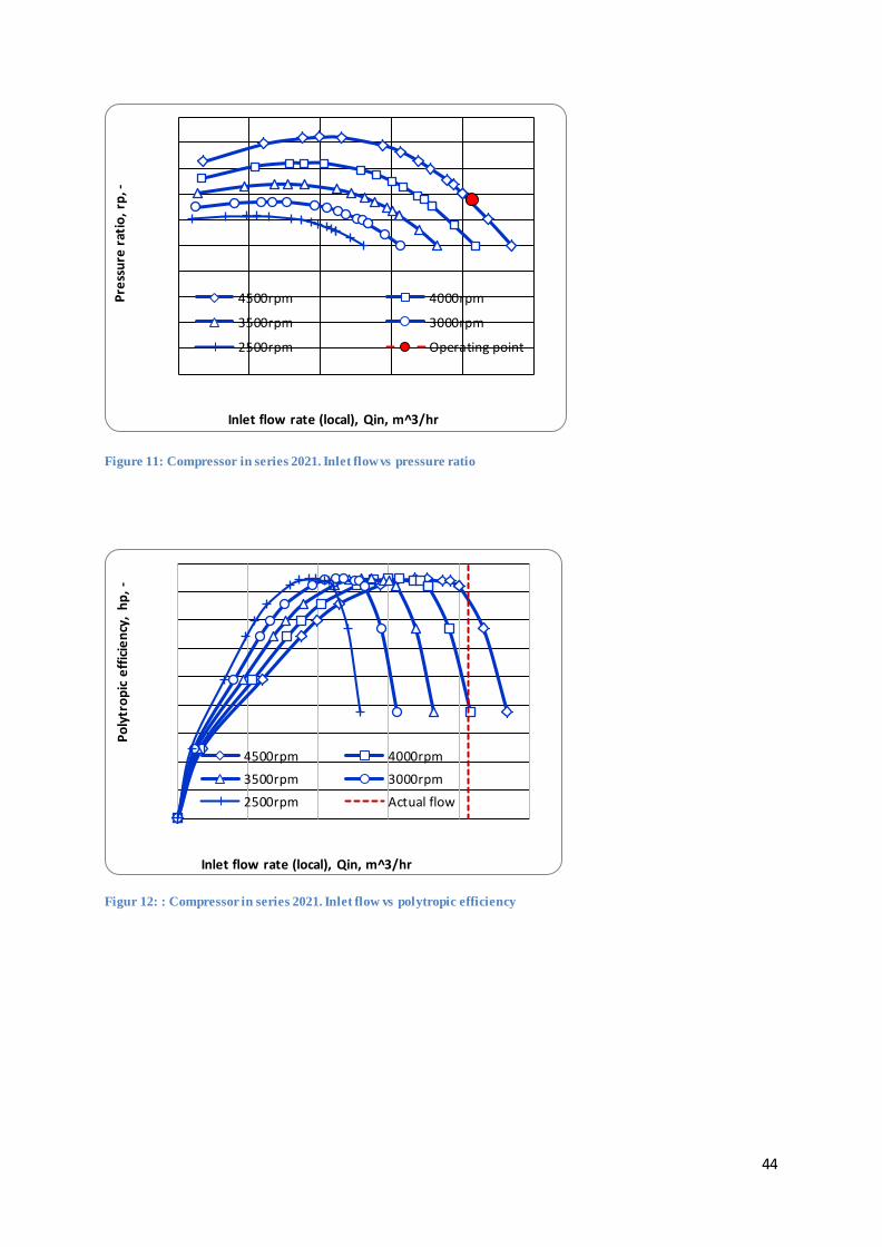
The results shows that from 2016-2021 the flow is too big for one single compressor to handle, so the
compressors need to be arranged in parallel. From 2021 the flow is reduced a lot, so now the main
parameter is the pressure ratio of the compressors. If the compressors are kept in parallel, the
limitation of the pressure ratio is exceeded. Therefore the arrangement is changed to series from 2021.
This will fix the compressor ratio, and also manage the total flow rate.
0
0,1
0,2
0,3
0,4
0,5
0,6
0,7
0,8R
eco
very
fa
cto
r (G
p/G
)
Year
Recovery factor L
Recovery factor M
Figure 8 Recovery factor for template L and M

12
3. Part B
In part A the main production model was established, a technical overview of the compressor
characteristics was given and Scenario A with no LPM was simulated. In part B, the dry gas
assumption was validated from part A, and the dry gas model was expanded to include condensate.
Further a thorough validation of the compressor characteristics was performed. Two new production
scenarios were the treated. In the first, scenario 1B, the production is subject to restrictions on what
pipes which can be used to transport the gas from the templates to the platform. In the second scenario,
2B, there are no restrictions, and in addition the production strategy for the templates was optimized.
Scenario 2B is the best-case scenario, and the production strategy developed is of interest in its own
right.
The economic analysis has two main objectives: One is to evaluate the NPV of the compression
project in each of the three scenarios. The second is to give the total NPV for each of the simulated
cases, showing how the conditions/assumptions on the production affect the total value of the project.
The report is concluded with a summary of conclusions and recommendations.
3.1 Material balance calculations based on black oil properties
In part A of the project one of our main assumptions was a dry gas model, and condensate was not
considered. To evaluate this assumption a modified black oil formulation was used instead of
traditional formulation.
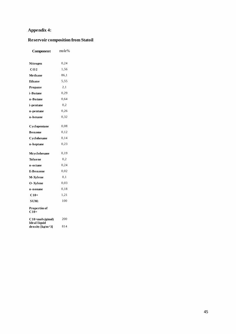
In order to calculate the amount of condensate produced from Gullfaks C, certain properties from the
condensate produced is needed. To generate these properties, HYSYS was used. Composition of the
gas- condensate in the reservoir was provided by Statoil, and can be viewed in the appendix 4. The
following equations and steps show the foundation of the calculations, and are included to give a
general overview of the method. Calculations done for oil from reservoir gas are taken into account
and the complete calculation method used can be viewed in appendix(4). It is important to specify that
the calculation method was implemented in a Excel sheet called Material Balance (MATBAL) made
by PhD Milan Stanko at NTNU, and that this sheet simply was used to generate the black oil
parameters by changing reservoir pressure using HYSYS. The calculations are based on the Whitson
balance.[8]
13
For the traditional BO formulation three properties is used to relate surface and reservoir volumes,
shown in equations 5-7:
(5)
(6)
(7)
“These three properties constitute the traditional black-oil PVT formulation, which has the
following assumptions:
1. Reservoir oil consists of two surface “components,” stock-tank oil and surface total separator
gas.
2. Reservoir gas does not yield liquids when brought to the surface.
3. Surface gas released from the reservoir oil has the same properties as the reservoir gas.
4. Properties of stock-tank oil and surface gas do not change during depletion of a reservoir.”
The modified Black Oil model includes an oil condensate, while still being simpler than solving a
problem using component by component basis. The four Modified Black Oil(MBO) PVT parameters,
oil formation volume factor (Bo) , solution gas-oil ratio (Rs), dry gas formation volume factor (Bgd),
solution oil-gas ratio (rs) are defined as
(8)
(9)
(10)
(11)

14
Where,
reservoir-oil volume,
volume of stock-tank oil produced from the reservoir oil,
volume of surface gas produced from the reservoir oil,
reservoir gas volume,
volume of surface gas produced from the reservoir gas,
stock-tank oil (condensate) produced from the reservoir gas.
From these definitions, a spreadsheet in HYSYS was made, and implemented further on in IPT-
Material balance. Table 2 shows the values generated in HYSYS, for different pressures. The
simulation was performed in steady state, so the pressures were changed manually for each pressure
step. Muo and Mug is the viscosity of the reservoir oil and reservoir gas respectively. Also densities
for each material stream is provided; denog, denoo, dengo and dengg. Gammao and gammag is
defined as:
(12)
(13)

15
Table 2 Black oil properties from HYSYS .
p Bo Bg Rs rs mu
o
mug deno
g
deno
o
gamma
o
deng
o
deng
g
gamma
g
bar
a
m3/Sm
3
m3/Sm
3
Sm3/Sm
3
Sm3/Sm
3
cp cp Kg/m3 Kg/m
3
- Kg/m
3
Kg/m
3
-
240 1,656 0,006 187,96 1,02E-
04
0,19
3
2,27
E-02
793,43
0
802,6
2
0,989 0,890 0,821 1,084
220 1,591 0,006 164,44 8,16E-
05
0,20
9
2,15
E-02
793,06
5
802,2
6
0,989 0,897 0,822 1,092
200 1,533 0,007 143,04 6,46E-
05
0,22
4
2,05
E-02
792,94 801,8
9
0,989 0,905 0,823 1,100
180 1,478 0,007 123,40 5,05E-
05
0,24
1
1,96
E-02
793,03 801,5
2
0,989 0,914 0,824 1,109
160 1,425 0,008 105,22 3,92E-
05
0,25
8
1,87
E-02
793,23 801,1
7
0,990 0,923 0,825 1,119
140 1,375 0,009 88,29 3,04E-
05
0,27
7
1,79
E-02
793,30 800,9
0
0,991 0,932 0,825 1,130
120 1,327 0,011 72,47 2,40E-
05
0,29
7
1,72
E-02
792,94 800,7
5
0,990 0,942 0,825 1,141
100 1,281 0,013 57,63 1,95E-
05
0,31
9
1,66
E-02
791,85 800,8
1
0,989 0,951 0,825 1,153
80 1,239 0,016 43,74 1,69E-
05
0,34
3
1,60
E-02
789,87 801,2
1
0,986 0,961 0,826 1,163
60 1,200 0,022 30,69 1,58E-
05
0,37
2
1,55
E-02
787,46 802,0
9
0,982 0,964 0,827 1,165

16
3.1.1 Results from IPT- Material balance
In the following section results from the MATBAL is shown. In MATBAL a comparison between dry
gas and wet gas can be plotted, and the difference can therefore be analyzed. Results from MATBAL
was further on implemented in the economic analysis to evaluate the condensate produced.
Figure 9: Gas condensate and dry gas production vs time for template L
Figure 10: Gas condensate and dry gas production vs time for template M
17
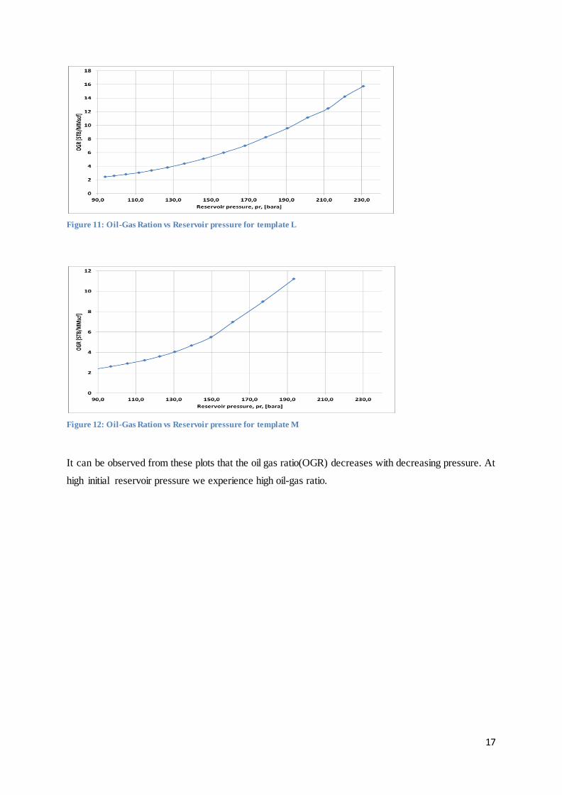
Figure 11: Oil-Gas Ration vs Reservoir pressure for template L
Figure 12: Oil-Gas Ration vs Reservoir pressure for template M
It can be observed from these plots that the oil gas ratio(OGR) decreases with decreasing pressure. At
high initial reservoir pressure we experience high oil-gas ratio.

18
Figur 13: Reservoir pressure and condensate production for template L
Figure 14: Reservoir pressure and condensate production for template M
In the Part A of the Gullfaks project a dry gas model was one of the main assumptions. In the reality
there is some amount of condensate coming out to the surface from the reservoir gas. In our

19
calculations the main goal was to find out the effect of wet gas and to check whether or not our dry gas
assumption was valid.
As shown in the plots there is a slight difference between the gas-condensate and dry gas models, but
the difference is so small that it is negligible. Therefore we concluded that our assumption is valid,
based on comparison of reservoir pressure and condensate production.
3.2 Wet gas compression
At high pressures and temperatures, the ideal gas behavior is not valid due to changes in fluid
properties. Therefore we need a correlation for this. In HYSYS, one option is to choose the Schultz
equation. This is a polytrophic calculation method which takes into account the real gas behavior. The
procedure assumes a polytrophic compression path based on averaged gas properties of inlet and outlet
conditions.
The presence of liquid increases the flow complexity in the compressor. Fluid properties may vary
through the compression process due to energy transfer between the phases. The dry gas performance
analysis becomes insufficient when analyzing wet gas compressor performance. A detailed analysis of
the fluid properties along the compression path is essential to assure correct calculations. The phase
exchange during wet gas compression is not accounted for when utilizing averaged gas properties as in
the Schultz procedure.
Another important thing is that the amount of liquid present in the compression process will reduce the
discharge temperature of the compressor. [9]
3.2.1 Compressor validation
As of today there exists no method of modeling a multiphase compressor. There are several
approaches on how to do it, but no general model implemented in a simulation program. One approach
of modeling the subsea process in Gullfaks south is to put a separator upstream the compressor. Here
the gas and liquid will be separated into two separated phases. Further on you insert a pump to pump
the liquid, and a compressor to compress the gas. The outlet streams of the compressor and the pump
get mixed together at the end, and now you can compare the total effect of the compressor and the
pump. An arrangement on how this could be done in HYSYS, is illustrated in the figure 15.

20
Figure 15 Reservoir stream separated in HYSYS
Another approach is to simulate the compressor in HYSYS as a wet compressor. One of the
differences between this approach, and the one mentioned above is that the cooling effect of the liquid
will now be present in the simulation.
To validate the compressor characteristics, a comparison with the Excel sheet provided by the Gullfaks
Village and a steady state simulation in HYSYS was done. The main goal of this comparison was to
check the cooling effect of the liquid in the wet gas, related to the constraint of the discharge
temperature of the compressor. Also a comparison of the power consumption was of interest.
The Excel sheet is based on test results from Framo Engineering, and calculates compression based on
dry gas behavior. The excel sheet uses ideal gas behavior, and the Z-factor to calculate the output
parameters of the compressor. The HYSYS model is based on the reservoir composition given by
Statoil, with an initial vapor phase fraction of 0,9619 and a liquid phase fraction of 0,0381. Peng
Robinson was used as equation of state.
Temperature of the inlet stream to the compressor was kept constant at 35°C. Suction pressure,
discharge pressure and flow rate was changed according to the flow optimization sheet from Excel.
For each compressor curve, the polytrophic efficiency was corrected for, by using the excel sheet.
One of the assumptions done in this comparison is that the polytrophic efficiency is the same for the
dry gas and the wet gas. Meaning that we neglect the effect the liquid in the wet gas will have on the
polytrophic efficiency.
For each simulation, values was taken from HYSYS, and implemented into Excel. From Excel the
polytropic effiency was taken, and used in HYSYS. Results were then compared. Only the main

21
results will be mentioned in the following sections. For all results, see appendix(...) Simulation was
performed for compressors arranged in parallel and series.
3.2.2 Wet gas compressors in parallel
For the compressor arrangement in parallel, a splitter was inserted to split the reservoir stream in half,
giving the compressors the same flow. A picture of the arrangement can be viewed in the figure 16. In
the figure the compressors turn yellow because of the liquid content in the gas.
Figure 16 Wet gas compressors in parallel in HYSYS
The two different methods give a large difference in discharge temperature. The discharge temperature
from Excel is throughout higher than the discharge temperature from HYSYS. The difference lies
between 14-41 %. The main reason for this is due to the cooling effect from the liquid.
The difference in power consumption was fairly small, 2-10%, where the power consumption from the
Excel sheet was higher throughout the comparison.
3.2.3 Wet gas compressors in series
In series, the compressors were arranged so that the middle pressure corresponded to the optimum in
two- stage compression. This is when the pressure ratios are equal (equation 14-15) [10]
(14)
Rearranging this equation we get
√ (15)
Where:
P1: Suction pressure of first compressor
P2: Middle pressure between compressors
P3: Discharge of second compressor
22
Because of limitations for the Excel sheet, only the first compressor in series was evaluated. The
simulation in HYSYS is illustrated in figure 17.
Figure 17 Wet gas compressors in series in HYSYS.
The results show a higher discharge temperature from the Excel sheet compared to the simulation in
HYSYS. The difference is between 9-30%. Somewhat a lower difference compared to the parallel
simulation, but still significant. Again the cooling effect of the liquid is the main factor why the
discharge temperature from HYSYS is lower.
The difference in power consumption was 3-6%, where the power consumption from the Excel sheet
was higher throughout the comparison.
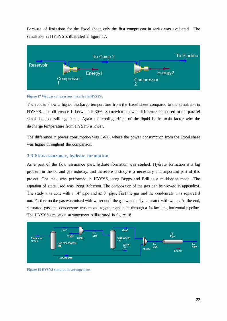
3.3 Flow assurance, hydrate formation
As a part of the flow assurance part, hydrate formation was studied. Hydrate formation is a big
problem in the oil and gas industry, and therefore a study is a necessary and important part of this
project. The task was performed in HYSYS, using Beggs and Brill as a multiphase model. The
equation of state used was Peng Robinson. The composition of the gas can be viewed in appendix4.
The study was done with a 14” pipe and an 8” pipe. First the gas and the condensate was separated
out. Further on the gas was mixed with water until the gas was totally saturated with water. At the end,
saturated gas and condensate was mixed together and sent through a 14 km long horizontal pipeline.
The HYSYS simulation arrangement is illustrated in figure 18.
Figure 18 HYSYS simulation arrangement

23
A phase envelope was made for the reservoir gas, to check the hydrate formation curve. From the
curve it can be seen that the hydrate formation temperature is approximately 25°C. This means that
hydrates will form if the temperature drops below 25°C, in the 14 km pipeline. The phase envelope
taken from HYSYS is illustrated in figure 19.
Figure 19 Phase envelope of reservoir gas from HYSYS
In the analysis a constant seabed temperature of 4°C was assumed [9], and also the riser was
neglected.

24
3.3.1 14” Pipeline
The fixed parameters for the 14” pipe is given in table 3. Temperature and pressure of the gas and
condensate entering the pipeline was set to 90°C and 73 bara respectively.
Table 3 Fixed parameters of 14” pipe
14” pipe
Length [km] 14
Elevation change [m] 0
Outer diameter [mm] 355,6
Inner diameter [mm] 320,0
Material Mild steel
Roughness [m] 4,572e-05
Pipe wall conductivity [W/mK] 45
Overall seawater temperature [°C] 4
During the simulation, sensitivity analysis was done by changing flow rate and overall heat transfer
coefficient. The flow rates was taken from the flow optimization part, and varied between 2,5MSm3/d
- 5,0MSm3/d. Minimum overall heat transfer coefficient was chosen to be 1,0 W/m
2K. A step of 1,0
W/m2K was used in the sensitivity analysis.
From the results of the sensitivity analysis it can be shown that hydrates start forming when the overall
heat transfer coefficient is increased to 7.0. This happens when the flow is 2.5MSm3/d, and the
temperature out of the pipeline is then 22.89°C.
3.3.2 8” pipeline
The same study was done for the 8” pipeline. The fixed parameters for the 8” pipeline are given in
table 4. Temperature and pressure of the gas and condensate entering the pipeline was set to 90°C and
73 bara respectively.

25
Table 4 Fixed parameters of 8” pipe
8” pipe
Length [km] 14
Elevation change [m] 0
Outer diameter [mm] 203,2
Inner diameter [mm] 197,0
Material Mild steel
Roughness [m] 4,572e-05
Pipe wall conductivity [W/mK] 45
Overall seawater temperature [°C] 4
During the simulation, sensitivity analysis was done by changing flow rate and overall heat transfer
coefficient. The flow rates was taken from the flow optimization part, and varied between 0,4MSm3/d
– 1,4MSm3/d. Minimum overall heat transfer coefficient was chosen to be 0,5 W/m
2K. A step of 0,5
W/m2K was used in the sensitivity analysis.
From the results of the sensitivity analysis it can be shown that hydrates start forming when the overall
heat transfer coefficient is increased to 2.0. This happens when the flow is 0.4 MSm3/d, and the
temperature out of the pipeline is then 23.72°C.
Table 5 Results for both 14" and 8" pipe
14” 8”
OHTC [W/m2K] 7 2
Flow rate [MSm3/d] 2,5 0,4
Outlet temperature [°C] 22,9 23,7
3.4 Production management in different scenarios
While previous sections have been centered on aspects of our model and technical investigations
related to the compressor, the rest of the report will focus on production management. More

26
specifically, in addition to Scenario A, two more scenarios are simulated with the model. The first one,
Scenario 1B, is straightforward to simulate, and only a brief discussion of this scenario is given.
Scenario 2B however, is a best-case scenario interesting in its own right, and a detailed description is
given.
Each of the three scenarios has two subcases: one with subsea compression and one without, where all
of the other conditions (production strategy, LPM or what pipes you are using) are fixed. There are
thus six cases in total. Simulating all these cases serves two purposes:
1. One gets the NPV of the compressor project under different operating conditions, giving a
more nuanced view of how robust the compressor investment is.
2. One gets the NPV for the total project under different operating conditions, showing the
effect of the differences in the cases compared to the project as a whole.
3.4.1 Modifying the Excel model from part A
While the model established in part A is good and outputs realistic numbers, some aspects were
changed in part B.
In part A, flows were assumed to mix in the towhead, but it later became clear that there is no mixing3,
and the model was changed accordingly. Mixing at the towhead before sending the flow through the
14 km pipes has the benefit of equalizing flows, meaning less pressure loss. Note also that mixing at
towhead will automatically make all seven wellhead pressures equal at the end of the natural plateau,
as the pressure loss is negligible in the flow lines connecting the templates with the towhead.
In Scenario 1B and 2B the pipes that are used changes, and when compression starts, one has to solve
for the flow distribution in the pipes going out of the compressor. Nature will of course arrange itself
so as to make the pressures at the end of the pipes equal. If two identical 14” pipes are used, the flow
will just split in half. Let’s consider the case with one 14”. This is the situation in Scenario 1B. Going
back to the equation governing pressure loss: (
) , the flow distribution is found with
simple algebra
(
)
(16)
Where is the total flow rate, is the rate through the 8” etc. Here will be the separator
pressure, while is the pressure at the compressor outlet. Other situations, for example the case with
two 14”s and one 8” as in Scenario 2B, is handled similarly.
3 Statoil/FRAMO staff in Bergen

27
As previously mentioned, the choke is what makes it possible to control the rates during the natural
plateau. The original model in part A assumes subsea choking, but this was later dropped, and the
model was changed to implement platform choking. The main difference in the pressure calculations
from part A is that to find the pressure difference over the choke, calculations are done upstream
instead of downstream. A question that arises is what the effect choking on the platform contra the
seabed has. One obvious effect is of course that it raises the pressure of the gas in the pipes on its way
to the platform. We haven’t investigated what effect this has4, but we stress that the placement of the
chokes doesn’t affect how long one can sustain the natural plateau. This is basically because placing
the chokes at the platform and having them fully open, is indistinguishable from placing the chokes at
the seabed and having them fully open.5
Finally, in Scenario 1B and Scenario 2B, low-pressure modification (LPM) is used. Compression is a
way to add pressure energy to the flow. Lowering the separator pressure reduces the pressure energy
required after transport to the platform. The default high-pressure separation is set to 65 bara, and this
is lowered to 25 bara over the period of a year. It is always initialized at the point where the plateau
would have otherwise ended. The result of performing low pressure modification is an extension of the
natural plateau with a production of 10 MSm3/day.
3.4.2 Scenario 1B: Shutting down one of the pipes in 2015
In this scenario high-pressure gas from the N-template will occupy the pipeline from the M-template
in 2015, which means that the gas from the M-template will have to go through the 8” from that point
on. Up to that point flows are as usual sent through separate 14” pipes. There will be an economical
loss from this when losing a pipe, since this means that more flow has to go through the remaining
pipes, increasing pressure loss due to friction. This means that total flow has to be lowered to
compensate, and the model verifies this. The simulation shows that the natural plateau can be
maintained until compression installation, if we lower the total flow to 9.85MSm3/day at the start of
2015. After compression installation, the production of course goes back up to 10MSm3/day. It may be
possible to do some kind of pressure analysis as above, preventing one from doing this slight lowering
of the plateau in the months before compressor installation, but this has not been investigated further.
3.4.1 Scenario 2B: The best case - finding an optimal production strategy
The overall goal of the Gullfaks village is to increase the recovery factor and value of the Gullfaks
field. This motivates the flow optimization performed, where all the value-enhancing technology (e.g.
the compressor) is utilized at our disposal, and come up with an optimal production strategy. To be
more specific, the optimization is as given:
4 Our chief technical supervisor, Professor Golan, indicated possible effects related to slugging. 5 This may be either obvious or unclear. The point is that placement of chokes won’t affect the simulation results.

28
Objective : Maximize the NPV of the project.
Assumptions : The 8” can be used freely; subsea compression is started at the end of the
natural plateau; LP-modification is started at the end of the compression plateau.6 Production
is stopped when the total flow drops to 5 MSm3/day.
In reality, Statoil has already decided on using both subsea compression and LP-modification, and
therefore it is interesting to optimize this case.
To optimize production, a good strategy of producing the fields is needed. A critical factor in this
respect is pressure loss of the gas between the reservoir and the platform; indeed the whole point of
installing the subsea compressor is to add pressure energy to the flow. In doing this, there has been
used intuition coming from the equation governing pressure loss in the pipe, (
) ,
where is the flow rate, is a constant depending on the pipe, and and are respectively the
initial and final pressure. This is a nonlinear equation, but it is easier to assess the pressure drop
if we linearize it using that the ratio
at our scales, to get
(
)
(17)
From equation 13 it can be seen that the pressure loss goes approximately quadratically with the flow
and inversely with the initial pressure.
The goal of the project is to maximize the NPV, and since the time-value of money decreases, a dollar
today is better than a dollar tomorrow. Also the gas prices are projected to decline, so one should
definitely strive to get out as much gas as possible early on. This reasoning shows that to get a high
NPV, it is preferable with a long plateau, and this has been the main focus of the optimization.
Sustaining the natural plateau for as long as possible also has other benefits, both since compression in
practice costs money, and because it provides extra time to deal with contingencies, for instance start-
up problems of the compressor.
What can be read out of the linearized pressure equation is this: to minimize the total pressure loss
with a fixed total flow rate, the flow in the flow in the pipes should be equalized. The model shows
that the largest pressure drop of the gas on its way to the platform is through the actual wells (the 7”
tubing). Since the ratio of the number of wells in the L- and M-templates is 4/3, the most pressure-
economical production is to produce from the templates roughly the same ratio, which during the
plateau amounts to about 6 MSm3/day from M-template and 4 MSm
3/day from the L-template. These
are precisely the ”target rates” given in the project description from Statoil. The problem which
becomes apparent after studying the results from the part A simulation in the Appendix is that since
6 In particular, we don’t optimize the timing of LP-modification.
29
the M-reservoir is depleted relatively faster than the L-reservoir, even if the production starts out with
the 4/3-ratio, the production rate from L has to increase to maintain the plateau.
The key point in our optimized strategy is to not try to use the 4/3-ratio for the rates throughout the
natural plateau. In the early years, when the reservoir pressure is still high, one can choke as one wants
and still produce 10 MSm3/day, because the reservoir pressure in our model only depends on how
much we have depleted compared to the GIIP. What one should strive for is to have this “pressure-
efficient” 4/3-ratio at the end of the natural plateau, and it is this criterion that guides us when deciding
how to choke.
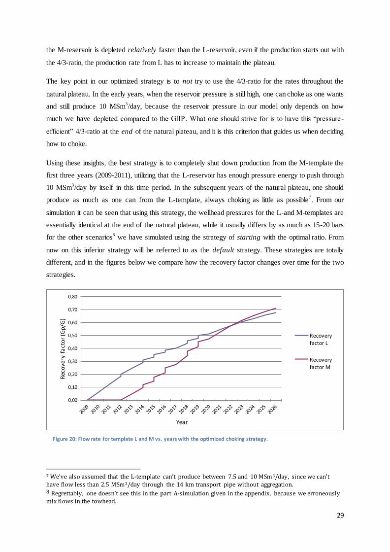
Using these insights, the best strategy is to completely shut down production from the M-template the
first three years (2009-2011), utilizing that the L-reservoir has enough pressure energy to push through
10 MSm3/day by itself in this time period. In the subsequent years of the natural plateau, one should
produce as much as one can from the L-template, always choking as little as possible7. From our
simulation it can be seen that using this strategy, the wellhead pressures for the L-and M-templates are
essentially identical at the end of the natural plateau, while it usually differs by as much as 15-20 bars
for the other scenarios8 we have simulated using the strategy of starting with the optimal ratio. From
now on this inferior strategy will be referred to as the default strategy. These strategies are totally
different, and in the figures below we compare how the recovery factor changes over time for the two
strategies.
7 We’ve also assumed that the L-template can’t produce between 7.5 and 10 MSm3/day, since we can’t have flow less than 2.5 MSm3/day through the 14 km transport pipe without aggregation. 8 Regrettably, one doesn’t see this in the part A-simulation given in the appendix, because we erroneously mix flows in the towhead.
0,00
0,10
0,20
0,30
0,40
0,50
0,60
0,70
0,80
Rec
ove
ry f
act
or
(Gp
/G)
Year
Recoveryfactor L
Recoveryfactor M
Figure 20: Flow rate for template L and M vs. years with the optimized choking strategy.
30
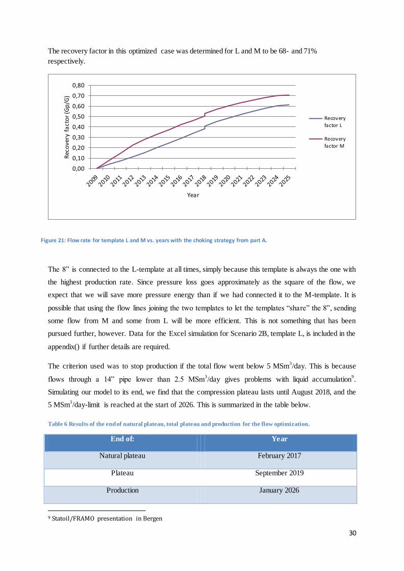
The recovery factor in this optimized case was determined for L and M to be 68- and 71%
respectively.
The 8” is connected to the L-template at all times, simply because this template is always the one with
the highest production rate. Since pressure loss goes approximately as the square of the flow, we
expect that we will save more pressure energy than if we had connected it to the M-template. It is
possible that using the flow lines joining the two templates to let the templates “share” the 8”, sending
some flow from M and some from L will be more efficient. This is not something that has been
pursued further, however. Data for the Excel simulation for Scenario 2B, template L, is included in the
appendix() if further details are required.
The criterion used was to stop production if the total flow went below 5 MSm3/day. This is because
flows through a 14” pipe lower than 2.5 MSm3/day gives problems with liquid accumulation
9.
Simulating our model to its end, we find that the compression plateau lasts until August 2018, and the
5 MSm3/day-limit is reached at the start of 2026. This is summarized in the table below.
Table 6 Results of the end of natural plateau, total plateau and production for the flow optimization.
End of: Year
Natural plateau February 2017
Plateau September 2019
Production January 2026
9 Statoil/FRAMO presentation in Bergen
0,00
0,10
0,20
0,30
0,40
0,50
0,60
0,70
0,80
Rec
ove
ry f
act
or
(Gp
/G)
Year
Recovery
factor L
Recovery
factor M
Figure 21: Flow rate for template L and M vs. years with the choking strategy from part A.

31
Stopping the production when reaching 5 MSm3/day is of course a major restriction in our model, but
we have later gotten indications that Statoil’s own simulation has been run several years longer.
According to our findings, this is impossible with the lower flow limit we have been using. Therefore
there has to be a way to avoid the problem of flow aggregation. One idea we have to achieve this is to
utilize that installing the compressor also means that you will have a manifold before the towhead, as
illustrated in the compressor sketch in part A. Therefore, it is possible to shut down one of the 14”s
and send the flow just through the 8” and the remaining 14”, increasing the flow rate through these
pipe. You will lose more pressure energy this way, but you can keep on producing longer. If this for
some reason does not work, and if it is economically viable, there is plenty of time to develop new
technology to deal with the aggregation problem before 2026.
As a final way to test our optimized production strategy, we’ve compared it with the default
production strategy in a ’zero-case’: a scenario without compressor, LPM, and just using the two 14”s
(together with the usual lower production limit). The optimized strategy had a recovery factor 0.76%
higher than the default strategy, with production in both cases stopping in January 2022.
We think it is interesting that playing with production rates and the 8” can extend the plateau by over
half a year. Of course everything depends on the correctness of our model; especially the equation for
the reservoir pressure. As a final observation, note that shutting down the pipe from the M-template in
2009-2011 frees this pipe up for other uses. This brings us over to Scenario 2, which is directly linked
to this.
4. Economical calculations
The economic analysis includes the evaluation of the economic value of compression in three different
scenarios and the economic value of production management in 6 different cases.
4.1 General economy
In order to evaluate the economic value of each of the different scenarios and to evaluate the economic
value of the compressor in our project an economic analysis was made with the following
assumptions:
Fixed 2013 Costs and oil/gas prices
1 USD = 6 NOK
Oil Price: 100 USD13/barrel
Gas Price: 2,30 NOK13/Sm3
Net Present Value estimated at 8% discount factor.
Taxation of net cash flow: 78%
No depreciation

32
All the assumptions were provided by Statoil. For the Capital Expenditures (CAPEX) the following
expenditures were taken into account:
Framo Engineering $156,380,316 USD for engineering, procurement and subsea compressor
construction.
Nexans $100,778,426 USD for 16.5 km of subsea power umbilical.
Subsea7 $70,000,000 USD for engineering, installation and commissioning of a 10 mile
integrated power service umbilical, a protection structure, a subsea compressor station,
pipeline spools and tie-ins.
1,000 MNOK for Low Pressure Modification.
The cost distribution for the Compressor CAPEX is 20% in year n-2, 40 % in year n-1 and 40
% in year n, where n is year the compressor started.
For the Operational Expenditures (OPEX) the analysis includes the following:
Operational Cost per year for Energy, CO2 and NOX provided by Statoil.
Sorco Contract for upgrading and replacement of control system, instrumentation and cables.
Electricity for compressor considering assuming an average power consumption of 7.5 MW,
and the price of kWh being 0,50 NOK.
For water production we assumed and water gas ratio (WGR) of 15 m3/million Sm
3 in 2009 and
increasing 0.25 m3/million Sm
3 per year.
Figure 22: Comparison of revenues from oil and gas
1,00E+04
1,00E+05
1,00E+06
1,00E+07
1,00E+08
1,00E+09
1,00E+10
2005 2010 2015 2020 2025 2030
USD
Calendar Years
Gas Revenues
Oil Revenues
33
Seeing as the revenues from oil are so small compared to the revenues from gas, the oil is simply
ignored in our calculations.
4.2 Evaluating the NPV of the compressor project in different scenarios
As previously stated, the aim of the economic analysis is to evaluate the value added by the subsea
compressor in three scenarios, which we summarize here:
Scenario A: Do not use LPM, use two 14” pipes, default production strategy
Scenario 1B: Use LPM, two 14” pipes and one 8” pipe, default production strategy
Scenario 2B: Use LPM, from 2015 use one 14” pipe and one 8” pipe, optimized production
strategy
The analysis in each of these scenarios is based on simulating two cases: one with compression and
one without, keeping other variables fixed. To find out what value the compression project has in the
different scenarios, revenues coming from the extra gas produced was used and then compared with
the CAPEX and OPEX for the project, discounted and taxed as above.
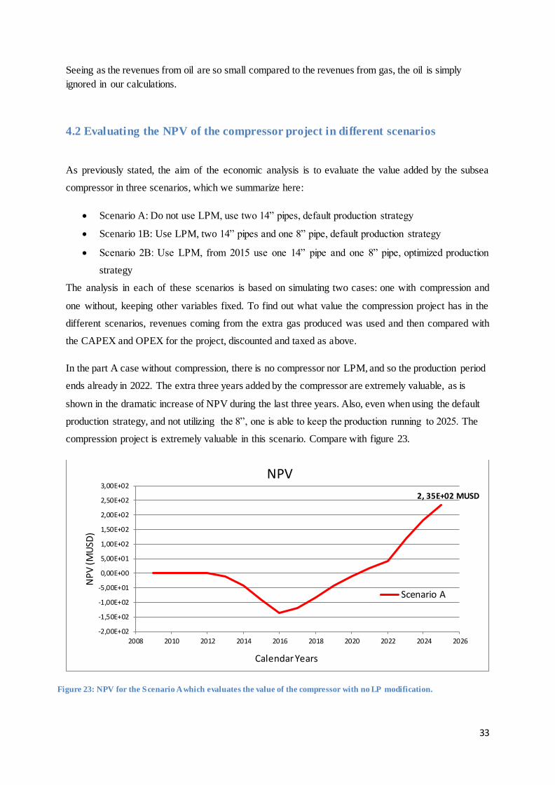
In the part A case without compression, there is no compressor nor LPM, and so the production period
ends already in 2022. The extra three years added by the compressor are extremely valuable, as is
shown in the dramatic increase of NPV during the last three years. Also, even when using the default
production strategy, and not utilizing the 8”, one is able to keep the production running to 2025. The
compression project is extremely valuable in this scenario. Compare with figure 23.
-2,00E+02
-1,50E+02
-1,00E+02
-5,00E+01
0,00E+00
5,00E+01
1,00E+02
1,50E+02
2,00E+02
2,50E+02
3,00E+02
2008 2010 2012 2014 2016 2018 2020 2022 2024 2026
NP
V (M
USD
)
Calendar Years
NPV
Scenario A
Figure 23: NPV for the Scenario A which evaluates the value of the compressor with no LP modification.
2, 35E+02 MUSD
34
Table 7 shows the Break Even and the Internal Rate of Return for Scenario A.
Table 7: Break even and internal rate of return (IRR), scenario A
Scenario Break Even IRR
A, compression 2020 26,30 %
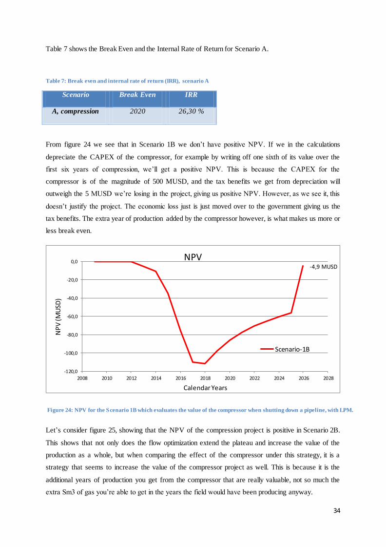
From figure 24 we see that in Scenario 1B we don’t have positive NPV. If we in the calculations
depreciate the CAPEX of the compressor, for example by writing off one sixth of its value over the
first six years of compression, we’ll get a positive NPV. This is because the CAPEX for the
compressor is of the magnitude of 500 MUSD, and the tax benefits we get from depreciation will
outweigh the 5 MUSD we’re losing in the project, giving us positive NPV. However, as we see it, this
doesn’t justify the project. The economic loss just is just moved over to the government giving us the
tax benefits. The extra year of production added by the compressor however, is what makes us more or
less break even.
Let’s consider figure 25, showing that the NPV of the compression project is positive in Scenario 2B.
This shows that not only does the flow optimization extend the plateau and increase the value of the
production as a whole, but when comparing the effect of the compressor under this strategy, it is a
strategy that seems to increase the value of the compressor project as well. This is because it is the
additional years of production you get from the compressor that are really valuable, not so much the
extra Sm3 of gas you’re able to get in the years the field would have been producing anyway.
-4,9 MUSD
-120,0
-100,0
-80,0
-60,0
-40,0
-20,0
0,0
2008 2010 2012 2014 2016 2018 2020 2022 2024 2026 2028
NP
V (M
USD
)
Calendar Years
NPV
Scenario-1B
Figure 24: NPV for the Scenario 1B which evaluates the value of the compressor when shutting down a pipeline, with LPM.

35
To sum up, the compression project seems to gravitate around an NPV of 0 if we use LPM and respect
the 5 Msm3/day lower flow limit, and doesn’t seem to be a robust investment under these restrictions.
We need to continue for additional years for the compression to be valuable.
4.2 Evaluating the production management scenarios.
In this section the total NPVs for all six cases are given. As pointed out earlier, this is interesting
because one gets the NPV for the total project under different operating conditions, showing the effect
of the differences in the cases compared to the scale of the entire project. In figure 26 the NPVs for the
cases are plotted as a function of time.
50,3 MUSD
-120,0
-100,0
-80,0
-60,0
-40,0
-20,0
0,0
20,0
40,0
60,0
2008 2010 2012 2014 2016 2018 2020 2022 2024 2026 2028
NP
V (M
USD
)
Calendar Years
NPV
Scenario 2B
Figure 25: NPV for the Scenario 2B which evaluates the value of the compressor with flow optimization.

36
The effects of no expenditures related to the compressor and LPM are seen in the early years for
Scenario A without compression, giving it the best NPV in the early years. After the natural plateau
has ended the scenarios with the value-enhancing technology begin to dominate.
Table 8: NPV and Recovery Factors for different scenarios.
Scenarios NPV (Billion
USD)
Recovery
Factor
A, no compression 2.53 0.508
A , compression 2.69 0.634
1B, no compression 2.85 0.633
1B, compression 2.86 0.677
2B, no compression 2.87 0.651
2B, compression 2.89 0.687
Table 8 really summarizes everything. This table also indicates the benefits of LPM, which adds a lot
of value to the project. Note that the value added to the project by the compressor is much higher if
0,00E+00
5,00E+02
1,00E+03
1,50E+03
2,00E+03
2,50E+03
3,00E+03
3,50E+03
2008 2010 2012 2014 2016 2018 2020 2022 2024 2026 2028
NP
V (M
USD
)
Calendar Years
NPV for Different Scenarios
Scenario A No CompressorScenario A CompressorScenario 1B No CompressorScenario 1B CompressorScenario 2B No CompressorScenario 2B Compressor
Figure 26: NPV plot showing the economic effect of producing in 6 different cases.

37
LPM isn’t used. Much of the benefits related to compression seem to drown in the value added by the
LPM.
Also, we see that the NPVs for the two cases within the same scenario are ordered in the correct way
according to the results from section 4.2.
5. Summary and recommendations
All in all, it seems that that our simple model was a good approximation to reality. The results we have
achieved seems reasonable and coherent.
Related to the performance of the compressor, a complete wet gas model would have been of great
value in this project. With this, more realistic simulations could have been done to evaluate the
performance of the compressor.
We have explored the NPV of the compression project under three different scenarios; in one of these
we have optimized the production strategy, and we have seen that it outperforms our so-called
‘default’-strategy. The 5 MSm3/day lower production limit we have used entails that the project will
end in 2025-2026. Our economic analysis indicates that the project is not economically robust, but it
seems that a lower flow limit will make the NPV positive. The critical factor is really how long the
project has been run. If it’s only run until the 5 MSm3/day limit, our conclusion is that the project is
not economically feasible.

38
List of Symbols, abbrevation and Quantities used
CAPEX Capital expenditure
Ct Tubing coefficient 7" (ID=6.094")
DPchoke Pressure difference over the choke
Error suction Difference between pressures when mixing flows at the compressor intake
(in reality 0)
Error ∆P2 Difference in ∆P fixed compressor and ∆P
GIIP Gas initially in place
GP Gas produced
∆GP Change in gas produced
GP/G(GIIP) Recovery factor
h Hour
kW Kilowatt
LPM Low-pressure modification
m Meter
N Compressor speed (rpm)
OPEX Operation expenditure
Plateau Period with total production 10 Msm3/day
Pi Initial reservoir pressure
Pr Reservoir pressure
Psep Separator pressure on platform
Ptowhead Towhead pressure
Ptemplate Template pressure
Psuck Suction pressure compressor
Psuck average Average suction pressure compressor
∆Pcomressor Pressure change over the compressor
P change in pressure
∆Pfixed Fixed change in pressure over the compressor
qf Flow rate from template L or M
qw Flow rate from well
qTot The total flow rate from template L and M
Rs Solution Gas oil Ratio
Sm3/day Standard cubic meters per day
T Temperature change
Z Compressibility factor
Td Discharge temperature
TR Temperature reservoir
C Degree centigrade
39
Literature 1. Statoil,
URL:http://www.statoil.com/no/ouroperations/explorationprod/ncs/gullfaks/pages/default.asp
x, Published 2007-09-26, 14:13 CET. Updated 2013-04-09, 08:19 CET. 26/4-2013
2. Statoil,URL:http://www.statoil.com/no/OurOperations/ExplorationProd/ncs/Gullfaks/Pages/G
ullfaksSouth.aspx, 10/4-2013
3. Powerpoint presentation given by Anne Margrete Solheim in Bergen 20.02.2013, Statoil
4. Statoil,URL:http://www.statoil.com/no/NewsAndMedia/PressRoom/Downloads/gullfaks_fiel
d_layout.jpg. 26/4-2013.
5. Offshore, A. Gilja, 6/5-2009,
URL:http://www.offshore.no/sak/24835_lovende_subsea_teknologikontrakt_til_framo 26/4-
2013
6. Offshore, J. Økland, 22/5-2012,
URL:http://www.offshore.no/sak/35196_tre_milliarder_girer_om_gullfaks_soer 26/4-2013
7. M, Golan, Sketch of process layout, 2013
8. Curtis H. Whitson and Michael R. Brule, 2000
9. S.C. Amundsen, “Wet Gas Compression”, NTNU, Master Thesis, 2009
10. Gudmundsson, JS. Kompresjon og Kompressorer, 2010
11. Boosting heating of subsea pipelines, 2003

40
List of appendix
Appendix 1
Relevant data from L and M template
Appendix 2
Excel sheet Part A
Appendix 3
Compressor map Part A
Appendix 4 Reservoir composition from Statoil
Appendix 5
HYSYS arrangement to generate black oil properties
Appendix 6
Results from comparison of dry gas model in excel and wet gas model in
HYSYS, Parallel
Appendix 7
Results from comparison of dry gas model in excel and wet gas model in
HYSYS, Series
Appendix 8
Results from sensitivity analyses regarding hydrate formation temperature
Appendix 9 Flow optimization Scenario 2B with compression, L-template
41
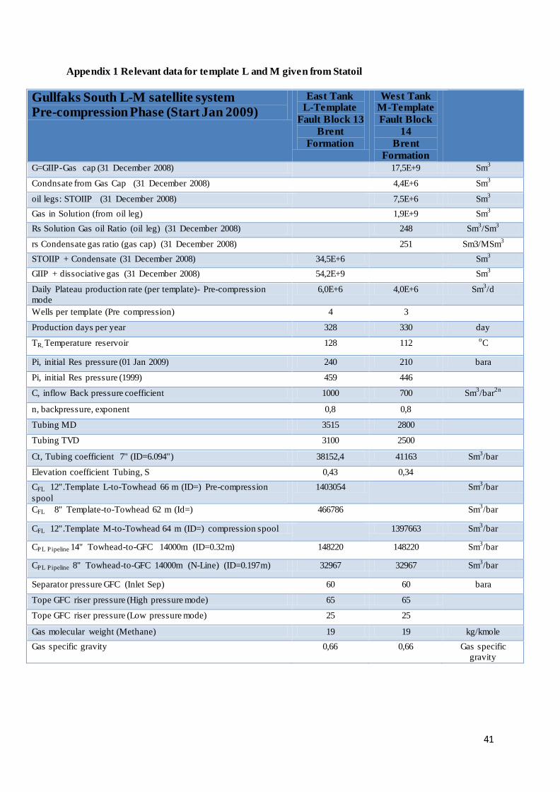
Appendix 1 Relevant data for template L and M given from Statoil
Gullfaks South L-M satellite system Pre-compression Phase (Start Jan 2009)
East Tank L-Template
Fault Block 13
Brent
Formation
West Tank M-Template
Fault Block
14
Brent
Formation
G=GIIP-Gas cap (31 December 2008) 17,5E+9 Sm3
Condnsate from Gas Cap (31 December 2008) 4,4E+6 Sm3
oil legs: STOIIP (31 December 2008) 7,5E+6 Sm3
Gas in Solution (from oil leg) 1,9E+9 Sm3
Rs Solution Gas oil Ratio (oil leg) (31 December 2008) 248 Sm3/Sm
3
rs Condensate gas ratio (gas cap) (31 December 2008) 251 Sm3/MSm3
STOIIP + Condensate (31 December 2008) 34,5E+6 Sm3
GIIP + dissociative gas (31 December 2008) 54,2E+9 Sm3
Daily Plateau production rate (per template)- Pre-compression
mode
6,0E+6 4,0E+6 Sm3/d
Wells per template (Pre compression) 4 3
Production days per year 328 330 day
TR, Temperature reservoir 128 112 oC
Pi, initial Res pressure (01 Jan 2009) 240 210 bara
Pi, initial Res pressure (1999) 459 446
C, inflow Back pressure coefficient 1000 700 Sm3/bar
2n
n, backpressure, exponent 0,8 0,8
Tubing MD 3515 2800
Tubing TVD 3100 2500
Ct, Tubing coefficient 7" (ID=6.094") 38152,4 41163 Sm3/bar
Elevation coefficient Tubing, S 0,43 0,34
CFL 12".Template L-to-Towhead 66 m (ID=) Pre-compression
spool
1403054 Sm3/bar
CFL 8" Template-to-Towhead 62 m (Id=) 466786 Sm3/bar
CFL 12".Template M-to-Towhead 64 m (ID=) compression spool 1397663 Sm3/bar
CPL Pipeline 14" Towhead-to-GFC 14000m (ID=0.32m) 148220 148220 Sm3/bar
CPL Pipeline 8" Towhead-to-GFC 14000m (N-Line) (ID=0.197m) 32967 32967 Sm3/bar
Separator pressure GFC (Inlet Sep) 60 60 bara
Tope GFC riser pressure (High pressure mode) 65 65
Tope GFC riser pressure (Low pressure mode) 25 25
Gas molecular weight (Methane) 19 19 kg/kmole
Gas specific gravity 0,66 0,66 Gas specific
gravity
42
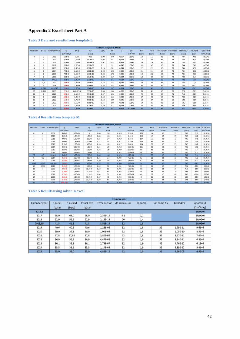
Appendix 2 Excel sheet Part A
Table 3 Data and results from template L
Table 4 Results from template M
Table 5 Results using solver in excel
Year cont ∆ time Calender year qf ∆ G p Gp Gp/G PR Z qw Pwf Pwh Psep 2x14'' Ptowhead Ptemp 12'' DpChoke q tot field
(Sm3/day) (Sm3) (bara) (Sm3/d) (bara) (bara) (bara) (bara) (bara) (bar) (Sm3/day)
0 0 2009 6,0E+6 0,00 0,00 0,00 240 0,957 1,5E+6 220 173 65 73 73,4 99,8 10,0E+6
1 1 2010 6,0E+6 2,0E+9 1,97E+09 0,04 231 0,953 1,5E+6 210 165 65 73 73,4 91,9 10,0E+6
2 1 2011 6,0E+6 2,0E+9 3,94E+09 0,07 222 0,948 1,5E+6 199 156 65 73 73,4 83,0 10,0E+6
3 1 2012 6,0E+6 2,0E+9 5,90E+09 0,11 212 0,945 1,5E+6 189 147 65 73 73,4 74,0 10,0E+6
4 1 2013 6,9E+6 2,3E+9 8,17E+09 0,15 201 0,941 1,7E+6 171 131 65 73 73,4 57,6 10,0E+6
5 1 2014 7,5E+6 2,5E+9 1,06E+10 0,20 190 0,938 1,9E+6 154 114 65 73 73,4 40,8 10,0E+6
6 1 2015 7,5E+6 2,5E+9 1,31E+10 0,24 178 0,936 1,9E+6 140 102 65 73 73,4 28,3 10,0E+6
7 1 2016 8,0E+6 2,6E+9 1,57E+10 0,29 167 0,934 2,0E+6 120 82 65 73 73,5 8,2 10,0E+6
7,5 0,5 2016,5 8,0E+6 1,3E+9 1,70E+10 0,31 161 0,934 2,0E+6 112 73 65 73 73,5 0,0 10,0E+6
8 0,5 2017 7,8E+6 1,3E+9 1,83E+10 0,34 155 0,934 1,9E+6 105 68 65 73 73,4 -5,2 10,0E+6
9 1 2018 7,6E+6 2,5E+9 2,08E+10 0,38 144 0,934 1,9E+6 90 53 65 73 73,4 -20,2 10,0E+6
9,645 0,645 2018,645 7,6E+6 1,6E+9 2,24E+10 0,41 137 0,934 1,9E+6 80 42 65 73 73,4 -31,7 10,0E+6
10 0,355 2019 7,3E+6 846,6E+6 2,33E+10 0,43 134 0,935 1,8E+6 78 41 65 73 72,8 -31,9 9,6E+6
11 1 2020 6,5E+6 2,1E+9 2,54E+10 0,47 125 0,936 1,6E+6 72 39 65 71 71,2 -31,9 8,5E+6
12 1 2021 5,9E+6 1,9E+9 2,73E+10 0,50 116 0,938 1,5E+6 67 38 65 70 70,0 -31,9 7,6E+6
13 1 2022 5,3E+6 1,7E+9 2,91E+10 0,54 109 0,940 1,3E+6 63 37 65 69 69,0 -31,9 6,8E+6
14 1 2023 4,8E+6 1,6E+9 3,06E+10 0,56 103 0,941 1,2E+6 59 36 65 68 68,2 -31,9 6,1E+6
15 1 2024 4,3E+6 1,4E+9 3,20E+10 0,59 97 0,943 1,1E+6 56 36 65 68 67,6 -31,9 5,4E+6
16 1 2025 3,9E+6 1,3E+9 3,33E+10 0,61 91 0,945 972,9E+3 54 35 65 67 67,1 -31,9 4,9E+6
East tank, template L, 4 Wells
Year cont ∆ time Calender year qf ∆ Gp Gp Gp/G PR Z qw Pwf Pwh Psep 2x14'' Ptowhead Ptemp 12'' DpChoke q tot field
(Sm3/day) (Sm3) (bara) (sm3/d) (bara) (bara) (bara) (bara) (bara) (bar) (Sm3/day)
0 0 2009 4,0E+6 0,0E+00 0 0,00 210 0,926 1,3E+6 178 146 65 73 73,3 72,7 10,0E+6
1 1 2010 4,0E+6 1,3E+09 1,3E+9 0,08 194 0,921 1,3E+6 158 129 65 73 73,3 56,2 10,0E+6
2 1 2011 4,0E+6 1,3E+09 2,6E+9 0,15 177 0,918 1,3E+6 137 111 65 73 73,3 37,8 10,0E+6
3 1 2012 4,0E+6 1,3E+09 4,0E+9 0,23 161 0,917 1,3E+6 116 92 65 73 73,3 18,5 10,0E+6
4 1 2013 3,1E+6 1,0E+09 5,0E+9 0,28 149 0,917 1,0E+6 114 93 65 73 73,3 19,2 10,0E+6
5 1 2014 2,5E+6 8,3E+08 5,8E+9 0,33 139 0,918 8,3E+05 111 91 65 73 73,3 18,0 10,0E+6
6 1 2015 2,5E+6 8,3E+08 6,6E+9 0,38 129 0,920 8,3E+05 99 81 65 73 73,3 7,3 10,0E+6
7 1 2016 2,0E+6 6,6E+08 7,3E+9 0,42 122 0,922 6,7E+05 98 81 65 73 73,2 7,3 10,0E+6
7,5 0,5 2016,5 2,0E+6 3,3E+08 7,6E+9 0,44 118 0,923 6,7E+05 93 77 65 73 73,2 3,3 10,0E+6
8 0,5 2017 2,2E+6 3,6E+08 8,0E+9 0,46 114 0,924 7,3E+05 83 68 65 73 73,2 -5,2 10,0E+6
9 1 2018 2,4E+6 7,8E+08 8,8E+9 0,50 105 0,928 7,8E+05 67 53 65 73 73,3 -20,3 10,0E+6
9,645 0,645 2018,645 2,4E+6 5,2E+08 9,3E+9 0,53 99 0,930 8,1E+05 54 41 65 73 73,3 -31,9 10,0E+6
10 0,355 2019 2,3E+6 2,7E+08 9,6E+9 0,55 96 0,931 7,7E+05 53 41 65 73 72,6 -32,0 9,6E+6
11 1 2020 2,0E+6 6,5E+08 10,2E+9 0,58 88 0,935 6,6E+05 50 39 65 71 71,1 -32,0 8,5E+6
12 1 2021 1,7E+6 5,6E+08 10,8E+9 0,62 81 0,938 5,7E+05 48 38 65 70 69,9 -32,0 7,6E+6
13 1 2022 1,5E+6 4,9E+08 11,3E+9 0,64 76 0,941 4,9E+05 46 37 65 69 68,9 -32,0 6,8E+6
14 1 2023 1,3E+6 4,2E+08 11,7E+9 0,67 71 0,944 4,3E+05 45 36 65 68 68,1 -32,0 6,1E+6
15 1 2024 1,1E+6 3,7E+08 12,1E+9 0,69 67 0,947 3,7E+05 44 36 65 68 67,5 -32,0 5,4E+6
16 1 2025 969,7E+3 3,2E+08 12,4E+9 0,71 63 0,949 3,2E+05 43 35 65 67 67,0 -32,0 4,9E+6
West tank, template M, 3 Wells
Calender year P suck L P suck M P suck ave Error suction ∆P Compressor rp comp ∆P comp fix Error ∆P 2 q tot field
(bara) (bara) (bara) (Sm3/day)
2016,5 10,0E+6
2017 68,0 68,0 68,0 2,39E-15 5,2 1,1 10,0E+6
2018 52,9 52,9 52,9 2,13E-14 20 1,4 10,0E+6
2018,65 41,3 41,3 41,3 8,51E-14 32 1,8 10,0E+6
2019 40,6 40,6 40,6 1,28E-06 32 1,8 32 1,99E-11 9,6E+6
2020 39,0 39,1 39,0 1,04E-04 32 1,8 32 1,05E-10 8,5E+6
2021 37,8 37,85 37,8 3,84E-05 32 1,8 32 3,97E-11 7,6E+6
2022 36,9 36,9 36,9 4,47E-05 32 1,9 32 3,34E-11 6,8E+6
2023 36,1 36,1 36,1 2,79E-07 32 1,9 32 4,76E-12 6,1E+6
2024 35,5 35,5 35,5 1,14E-05 32 1,9 32 5,89E-12 5,4E+6
2025 35,0 35,0 35,0 4,86E-12 32 1,9 32 4,66E-05 4,9E+6
Compressor
43
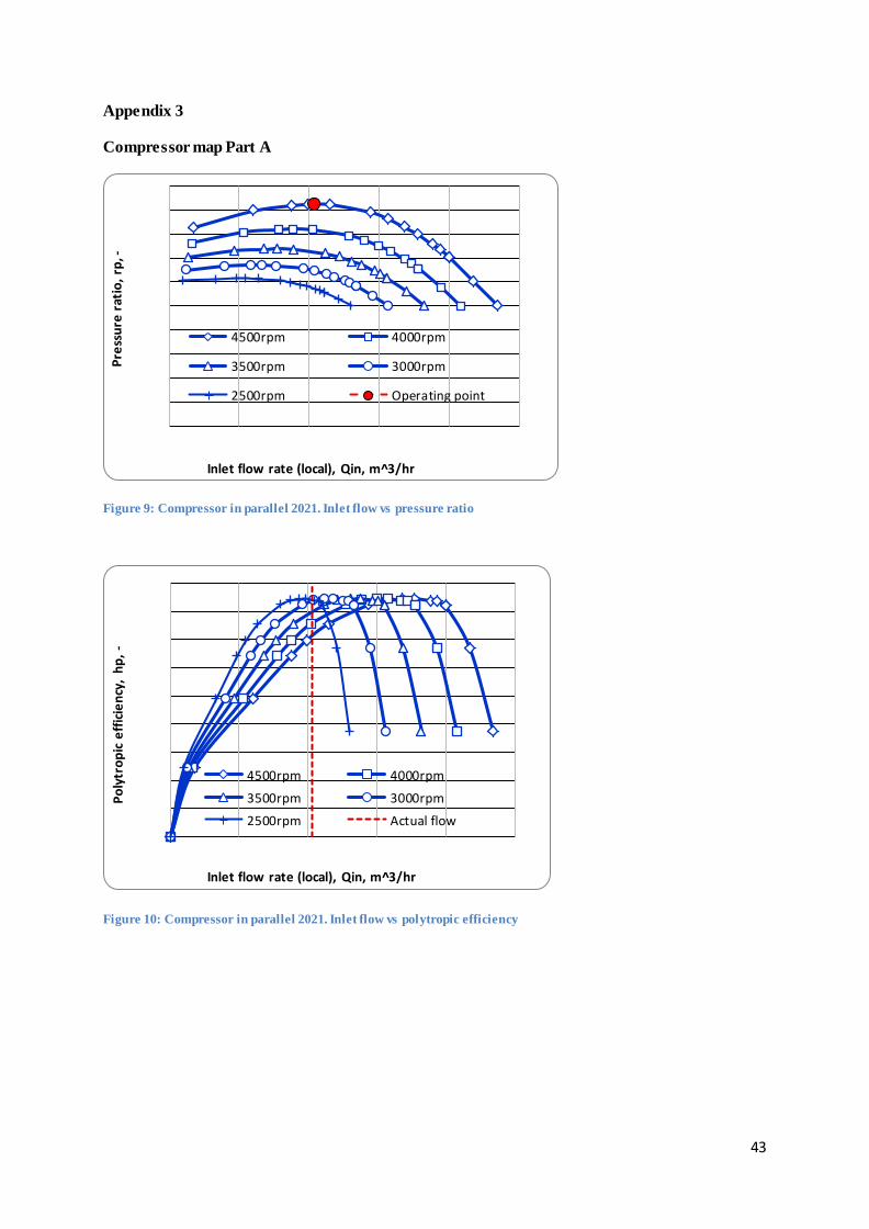
Appendix 3
Compressor map Part A
Figure 9: Compressor in parallel 2021. Inlet flow vs pressure ratio
Figure 10: Compressor in parallel 2021. Inlet flow vs polytropic efficiency
Pre
ssu
re r
atio
, rp
, -
Inlet flow rate (local), Qin, m^3/hr
4500rpm 4000rpm
3500rpm 3000rpm
2500rpm Operating point
Po
lytr
op
ic e
ffic
ien
cy,
hp
, -
Inlet flow rate (local), Qin, m^3/hr
4500rpm 4000rpm
3500rpm 3000rpm
2500rpm Actual flow
44
Figure 11: Compressor in series 2021. Inlet flow vs pressure ratio
Figur 12: : Compressor in series 2021. Inlet flow vs polytropic efficiency
Pre
ssu
re r
atio
, rp
, -
Inlet flow rate (local), Qin, m^3/hr
4500rpm 4000rpm
3500rpm 3000rpm
2500rpm Operating point
Po
lytr
op
ic e
ffic
ien
cy,
hp
, -
Inlet flow rate (local), Qin, m^3/hr
4500rpm 4000rpm
3500rpm 3000rpm
2500rpm Actual flow
45
Appendix 4:
Reservoir composition from Statoil
Component mole%
Nitrogen 0,24
CO 2 1,56
Methane 86,1
Ethane 5,55
Propane 2,1
i-Butane 0,29
n-Butane 0,64
i-pentane 0,2
n-pentane 0,26
n-hexane 0,32
Cyclopentane 0,08
Benzene 0,12
Cyclohexane 0,14
n-heptane 0,23
Mcyclohexane 0,19
Toluene 0,2
n-octane 0,24
E-Benzene 0,02
M-Xylene 0,1
O -Xylene 0,03
n-nonane 0,18
C10+ 1,21
SUM: 100
Properties of C10+
C10+molv.(g/mol) 200
Ideal liquid
density [kg/m^3] 814

46
Appendix 4: Calculation method for material balance
“The basis of calculation is 1bbl reservoir bulk volume. The conservation-of-mass equations for
single-cell material balance yields the following difference equations for reservoir-oil and –gas phases
during the time step with a change in average pressure from ( ) to ( ) .”
(Curtis H. Whitson and Michael R. Brule, 2000)
In our calculations 1 year is taken as a time step.
( ) ( ) and ( ) ( ) ,
where and incremental quantities of total surface oil and total surface gas, respectively,
produced during the timestep;
[ ( )
]
and
[
( )
]
and are in STB/bbl, and are in scf/bbl, and are in scf/bbl, is in scf/STB, is
in STB/scf, and is in / scf. Other quantities used in the material-balance procedure are
( )
Application of these relations for gas-condensate reservoirs is shown step by step.
1. Specify ( ) , total surface gas produced in scf/bbl of bulk volume.
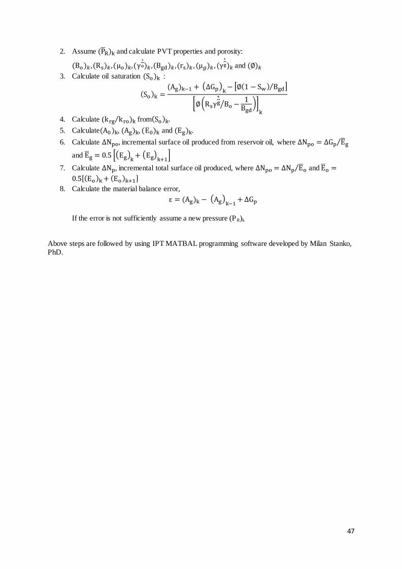
47
2. Assume ( ) and calculate PVT properties and porosity:
( ) ( ) ( ) (
) ( ) ( ) ( ) (
) and ( )
3. Calculate oil saturation ( ) :
( ) ( ) ( )
[ ( ) ⁄ ]
[ ( ⁄
)]
4. Calculate ( ⁄ ) from( ) .
5. Calculate( ) , ( ) , ( ) and ( ) .
6. Calculate incremental surface oil produced from reservoir oil, where ⁄
and [( ) ( ) ]
7. Calculate , incremental total surface oil produced, where ⁄ and
[( ) ( ) ]
8. Calculate the material balance error,
( ) ( )
If the error is not sufficiently assume a new pressure (PR)k Above steps are followed by using IPT MATBAL programming software developed by Milan Stanko, PhD.

Appendix 5:
HYSYS arrangement to generate black oil properties
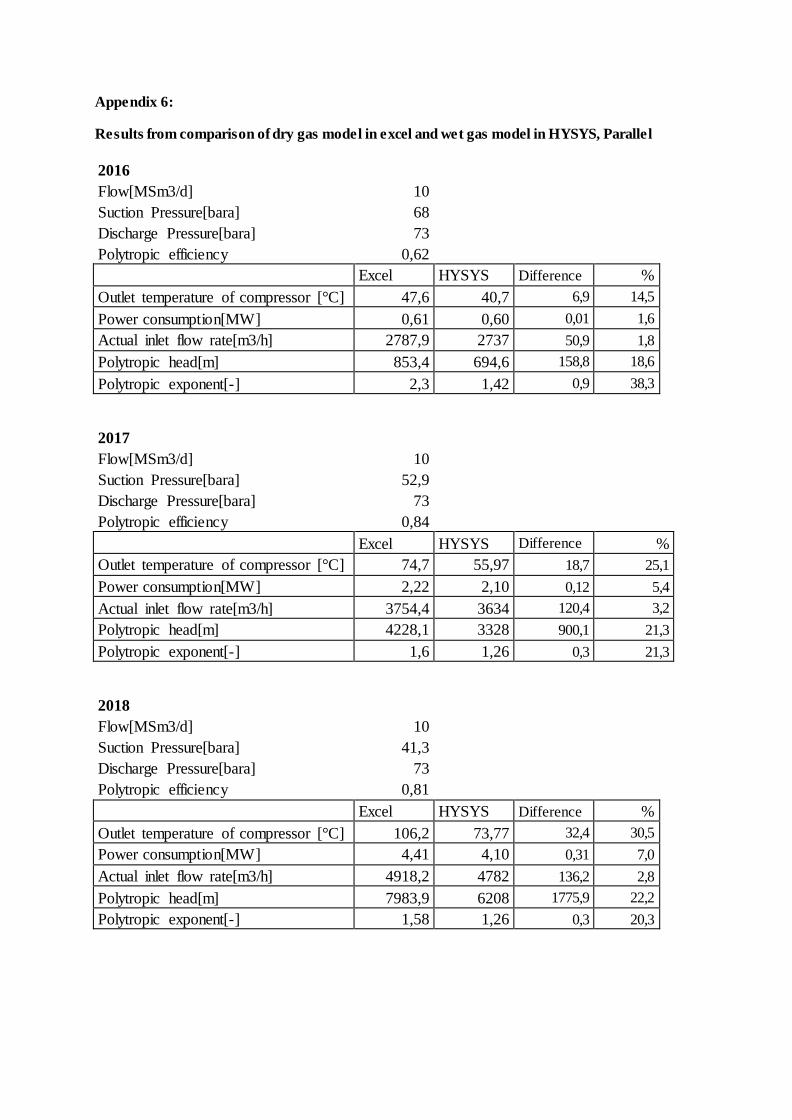
Appendix 6:
Results from comparison of dry gas model in excel and wet gas model in HYSYS, Parallel
2016
Flow[MSm3/d] 10 Suction Pressure[bara] 68 Discharge Pressure[bara] 73 Polytropic efficiency 0,62 Excel HYSYS Difference %
Outlet temperature of compressor [°C] 47,6 40,7 6,9 14,5
Power consumption[MW] 0,61 0,60 0,01 1,6
Actual inlet flow rate[m3/h] 2787,9 2737 50,9 1,8
Polytropic head[m] 853,4 694,6 158,8 18,6
Polytropic exponent[-] 2,3 1,42 0,9 38,3
2017
Flow[MSm3/d] 10 Suction Pressure[bara] 52,9 Discharge Pressure[bara] 73 Polytropic efficiency 0,84 Excel HYSYS Difference %
Outlet temperature of compressor [°C] 74,7 55,97 18,7 25,1
Power consumption[MW] 2,22 2,10 0,12 5,4
Actual inlet flow rate[m3/h] 3754,4 3634 120,4 3,2
Polytropic head[m] 4228,1 3328 900,1 21,3
Polytropic exponent[-] 1,6 1,26 0,3 21,3
2018
Flow[MSm3/d] 10
Suction Pressure[bara] 41,3
Discharge Pressure[bara] 73
Polytropic efficiency 0,81
Excel HYSYS Difference %
Outlet temperature of compressor [°C] 106,2 73,77 32,4 30,5
Power consumption[MW] 4,41 4,10 0,31 7,0
Actual inlet flow rate[m3/h] 4918,2 4782 136,2 2,8
Polytropic head[m] 7983,9 6208 1775,9 22,2
Polytropic exponent[-] 1,58 1,26 0,3 20,3

1
2019
Flow[MSm3/d] 9,6
Suction Pressure[bara] 40,6
Discharge Pressure[bara] 73
Polytropic efficiency 0,79
Excel HYSYS Difference %
Outlet temperature of compressor [°C] 110,7 75,73 35,0 31,6
Power consumption[MW] 4,5 4,17 0,33 7,3
Actual inlet flow rate[m3/h] 4802,9 4674,0 128,9 2,7
Polytropic head[m] 8273,32 6427 1846,3 22,3
Polytropic exponent[-] 1,60 1,27 0,3 20,6
2020
Flow[MSm3/d] 8,5 Suction Pressure[bara] 39 Discharge Pressure[bara] 71 Polytropic efficiency 0,75 Excel HYSYS Difference %
Outlet temperature of compressor [°C] 115,6 78,3 37,3 32,3
Power consumption[MW] 4,36 4,01 0,35 8,0
Actual inlet flow rate[m3/h] 4478,2 4322,0 156,2 3,5
Polytropic head[m] 8593,97 6619 1975,0 23,0
Polytropic exponent[-] 1,63 1,29 0,3 20,9
2021
Flow[MSm3/d] 7,6 Suction Pressure[bara] 37,8 Discharge Pressure[bara] 70 Polytropic efficiency 0,71 Excel HYSYS Difference %
Outlet temperature of compressor [°C] 121,7 82,7 39,0 32,0
Power consumption[MW] 4,27 4,02 0,25 5,9
Actual inlet flow rate[m3/h] 4129,3 4001,0 128,3 3,1
Polytropic head[m] 8911,2 7038 1873,2 21,0
Polytropic exponent[-] 1,67 1,31 0,4 21,6
2022
Flow[MSm3/d] 6,8
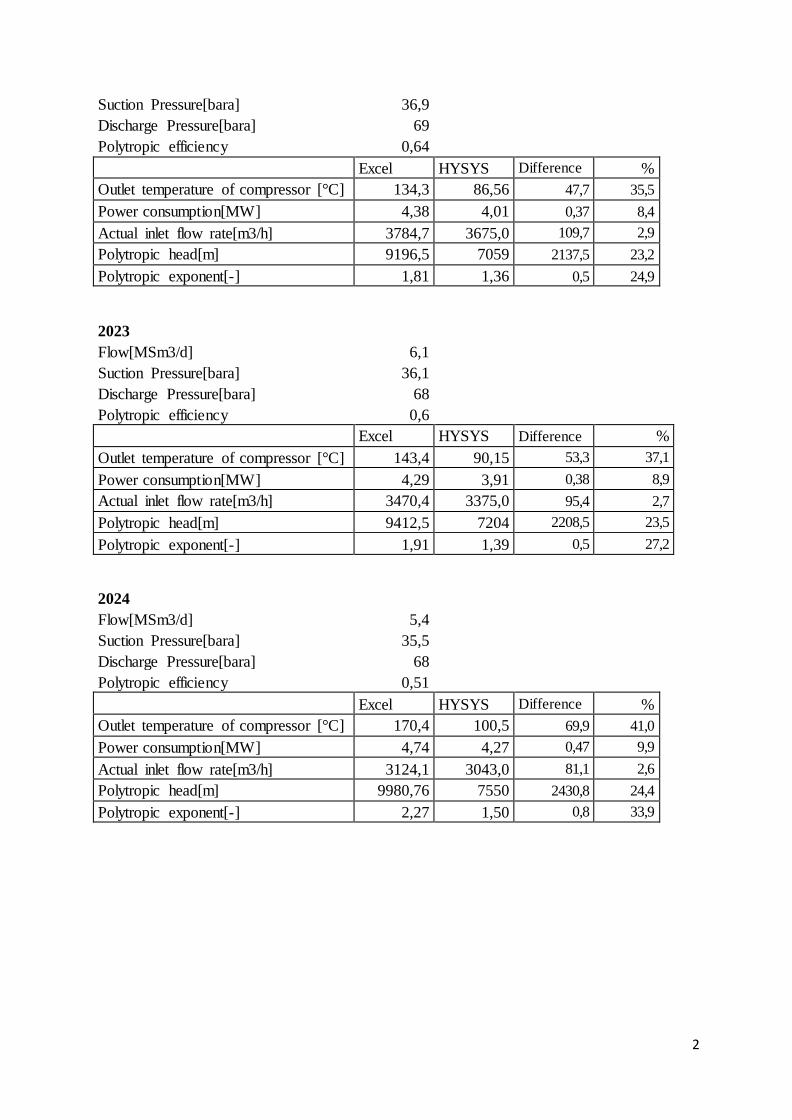
2
Suction Pressure[bara] 36,9
Discharge Pressure[bara] 69
Polytropic efficiency 0,64
Excel HYSYS Difference %
Outlet temperature of compressor [°C] 134,3 86,56 47,7 35,5
Power consumption[MW] 4,38 4,01 0,37 8,4
Actual inlet flow rate[m3/h] 3784,7 3675,0 109,7 2,9
Polytropic head[m] 9196,5 7059 2137,5 23,2
Polytropic exponent[-] 1,81 1,36 0,5 24,9
2023
Flow[MSm3/d] 6,1 Suction Pressure[bara] 36,1 Discharge Pressure[bara] 68 Polytropic efficiency 0,6 Excel HYSYS Difference %
Outlet temperature of compressor [°C] 143,4 90,15 53,3 37,1
Power consumption[MW] 4,29 3,91 0,38 8,9
Actual inlet flow rate[m3/h] 3470,4 3375,0 95,4 2,7
Polytropic head[m] 9412,5 7204 2208,5 23,5
Polytropic exponent[-] 1,91 1,39 0,5 27,2
2024
Flow[MSm3/d] 5,4 Suction Pressure[bara] 35,5 Discharge Pressure[bara] 68 Polytropic efficiency 0,51 Excel HYSYS Difference %
Outlet temperature of compressor [°C] 170,4 100,5 69,9 41,0
Power consumption[MW] 4,74 4,27 0,47 9,9
Actual inlet flow rate[m3/h] 3124,1 3043,0 81,1 2,6
Polytropic head[m] 9980,76 7550 2430,8 24,4
Polytropic exponent[-] 2,27 1,50 0,8 33,9

3
2025
Flow[MSm3/d] 4,9
Suction Pressure[bara] 35
Discharge Pressure[bara] 67
Polytropic efficiency 0,51
Excel HYSYS Difference %
Outlet temperature of compressor [°C] 177,3 104,2 73,1 41,2
Power consumption[MW] 4,6 4,14 0,46 10,0
Actual inlet flow rate[m3/h] 2875,3 2804,0 71,3 2,5
Polytropic head[m] 10053,1 7603 2450,1 24,4
Polytropic exponent[-] 2,41 1,54 0,9 36,1

4
Appendix 7:
Results from comparison of dry gas model in excel and wet gas model in HYSYS, Series
2016
Flow[MSm3/d] 10
Suction Pressure[bara] 68
Discharge Pressure[bara] 73
Middle Pressure 70,46
Polytropic efficiency 0,55
Excel HYSYS Difference %
Outlet temperature of compressor [°C] 42,0 38,08 3,9 9,3
Power consumption[MW] 0,69 0,67 0,02 2,9
Actual inlet flow rate[m3/h] 5575,9 5473,0 102,9 1,8
Polytropic head[m] 422,95 346,3 76,7 18,1
Polytropic exponent[-] 2,76 1,50 1,3 45,7
2017
Flow[MSm3/d] 10 Suction Pressure[bara] 52,9 Discharge Pressure[bara] 73 Middle Pressure 62,14 Polytropic efficiency 0,5 Excel HYSYS Difference %
Outlet temperature of compressor [°C] 68,4 50,41 18,0 26,3
Power consumption[MW] 3,74 3,54 0,20 5,3
Actual inlet flow rate[m3/h] 7508,8 7267,7 241,1 3,2
Polytropic head[m] 2094,6 1656 438,6 20,9
Polytropic exponent[-] 2,77 1,54 1,2 44,4
2018
Flow[MSm3/d] 10

5
Suction Pressure[bara] 41,3
Discharge Pressure[bara] 73
Middle Pressure 54,91
Polytropic efficiency 0,55
Excel HYSYS Difference %
Outlet temperature of compressor [°C] 86,0 60,72 25,3 29,4
Power consumption[MW] 6,31 6,00 0,31 4,9
Actual inlet flow rate[m3/h] 9836,4 9564,8 271,6 2,8
Polytropic head[m] 3880,8 3058,0 822,8 21,2
Polytropic exponent[-] 2,16 1,45 0,7 32,9
2019
Flow[MSm3/d] 9,6 Suction Pressure[bara] 40,6 Discharge Pressure[bara] 73 Middle Pressure 54,44 Polytropic efficiency 0,55 Excel HYSYS Difference %
Outlet temperature of compressor [°C] 87,7 61,52 26,2 29,9
Power consumption[MW] 6,26 5,90 0,36 5,8
Actual inlet flow rate[m3/h] 9605,7 9348,6 257,1 2,7
Polytropic head[m] 4006,7 3158,4 848,3 21,2
Polytropic exponent[-] 2,16 1,44 0,7 33,3
2020
Flow[MSm3/d] 8,5 Suction Pressure[bara] 39 Discharge Pressure[bara] 71 Middle Pressure 52,62 Polytropic efficiency 0,73 Excel HYSYS Difference %
Outlet temperature of compressor [°C] 74,1 56,53 17,6 23,7
Power consumption[MW] 4,23 3,98 0,25 5,9
Actual inlet flow rate[m3/h] 8952,4 8644,8 307,6 3,4
Polytropic head[m] 4054,3 3201,3 853,0 21,0
Polytropic exponent[-] 1,66 1,29 0,4 22,3
2021
Flow[MSm3/d] 7,6
Suction Pressure[bara] 37,8
Discharge Pressure[bara] 70
Middle Pressure 51,44

6
Polytropic efficiency 0,79
Excel HYSYS Difference %
Outlet temperature of compressor [°C] 71,3 55,82 15,5 21,7
Power consumption[MW] 3,58 3,39 0,19 5,3
Actual inlet flow rate[m3/h] 8258,6 8001,9 256,7 3,1
Polytropic head[m] 4153,1 3295,8 857,3 20,6
Polytropic exponent[-] 1,57 1,26 0,3 19,7
2022
Flow[MSm3/d] 6,8 Suction Pressure[bara] 36,9 Discharge Pressure[bara] 69 Middle Pressure 50,46 Polytropic efficiency 0,80 Excel HYSYS Difference %
Outlet temperature of compressor [°C] 71,4 55,9 15,5 21,7
Power consumption[MW] 3,21 3,05 0,16 5,0
Actual inlet flow rate[m3/h] 7569,5 7350,8 218,7 2,9
Polytropic head[m] 4217,0 3355,2 861,8 20,4
Polytropic exponent[-] 1,56 1,26 0,3 19,2
2023
Flow[MSm3/d] 6,1 Suction Pressure[bara] 36,1 Discharge Pressure[bara] 68 Middle Pressure 49,55 Polytropic efficiency 0,84 Excel HYSYS Difference %
Outlet temperature of compressor [°C] 69,6 55,2 14,4 20,7
Power consumption[MW] 2,74 2,60 0,14 5,1
Actual inlet flow rate[m3/h] 6940,7 6750,0 190,7 2,7
Polytropic head[m] 4254,7 3395,7 859,0 20,2
Polytropic exponent[-] 1,51 1,24 0,3 17,9
2024
Flow[MSm3/d] 5,4
Suction Pressure[bara] 35,5
Discharge Pressure[bara] 68
Middle Pressure 49,13
Polytropic efficiency 0,85
Excel HYSYS Difference %
Outlet temperature of compressor [°C] 70,6 55,72 14,9 21,1
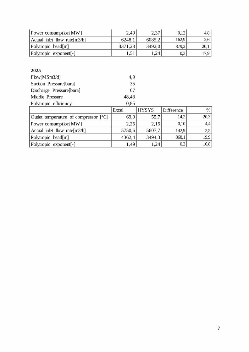
7
Power consumption[MW] 2,49 2,37 0,12 4,8
Actual inlet flow rate[m3/h] 6248,1 6085,2 162,9 2,6
Polytropic head[m] 4371,23 3492,0 879,2 20,1
Polytropic exponent[-] 1,51 1,24 0,3 17,9
2025
Flow[MSm3/d] 4,9 Suction Pressure[bara] 35 Discharge Pressure[bara] 67 Middle Pressure 48,43 Polytropic efficiency 0,85 Excel HYSYS Difference %
Outlet temperature of compressor [°C] 69,9 55,7 14,2 20,3
Power consumption[MW] 2,25 2,15 0,10 4,4
Actual inlet flow rate[m3/h] 5750,6 5607,7 142,9 2,5
Polytropic head[m] 4362,4 3494,3 868,1 19,9
Polytropic exponent[-] 1,49 1,24 0,3 16,8

8
Appendix 8:
Results from sensitivity analyses regarding hydrate formation temperature.
For the 14" pipeline
Overall Heat Transfer Coefficient [W/m2K] = 1,0
Molar Flow [kmol/h] Flow Rate[MSm3/d]
Temperature of gas out of pipeline
[°C]
4400 2,5 70,38
5300 3,0 71,99
6170 3,5 72,49
7050 4,0 72,05
7920 4,5 70,27
8810 5,0 65,09
Overall Heat Transfer Coefficient [W/m2K] = 2,0
Molar Flow [kmol/h] Flow Rate[MSm3/d]
Temperature of gas out of pipeline
[°C]
4400 2,5 57,58
5300 3,0 60,78
6170 3,5 62,54
7050 4,0 63,15
7920 4,5 62,37
8810 5,0 58,34
Overall Heat Transfer Coefficient [W/m2K]
= 3,0
Molar Flow [kmol/h] Flow Rate[MSm3/d]
Temperature of gas out of pipeline
[°C]
4400 2,5 47,25
5300 3,0 51,28
6170 3,5 53,92
7050 4,0 55,35
7920 4,5 55,34
8810 5,0 52,17
Overall Heat Transfer Coefficient [W/m2K]
= 4,0
Molar Flow [kmol/h] Flow Rate[MSm3/d]
Temperature of gas out of pipeline
[°C]
4400 2,5 39,28
5300 3,0 43,5
6170 3,5 46,57
7050 4,0 48,49
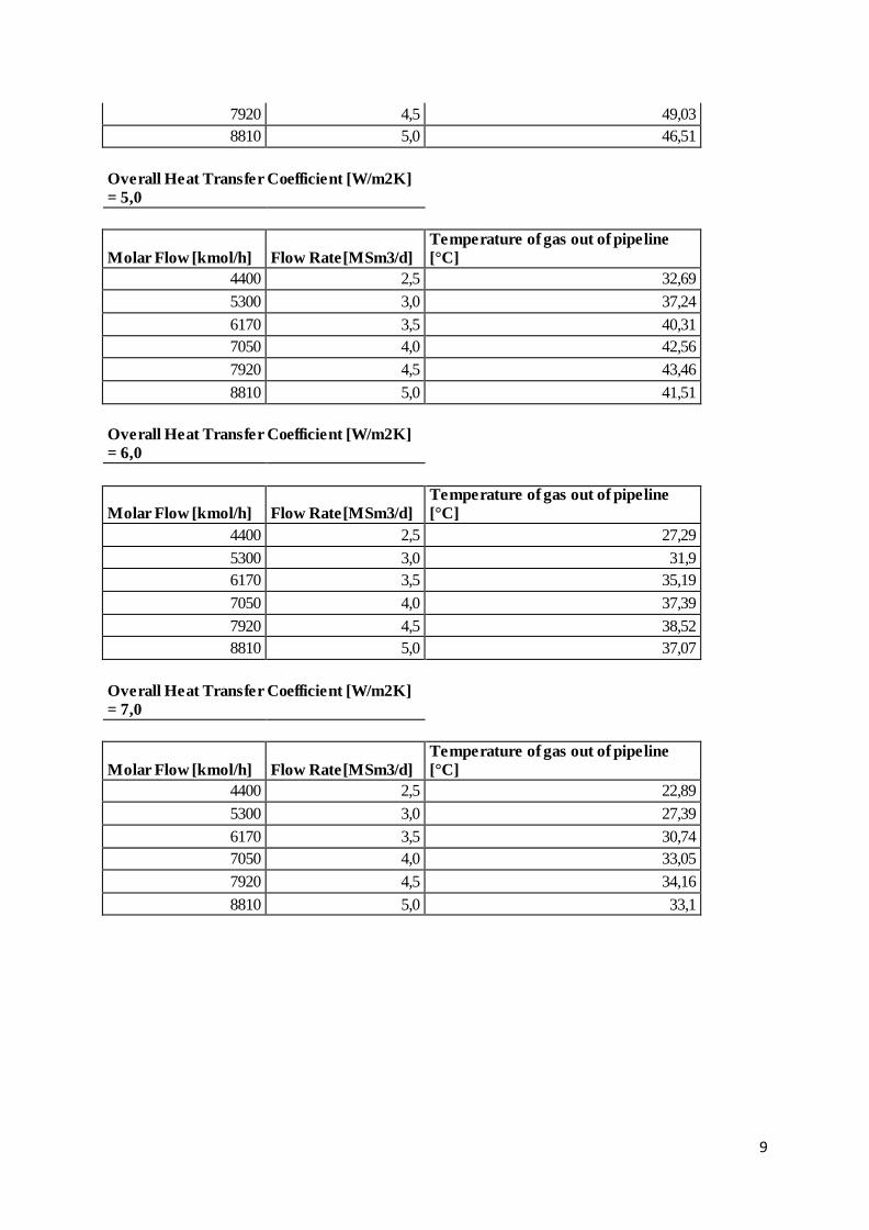
9
7920 4,5 49,03
8810 5,0 46,51
Overall Heat Transfer Coefficient [W/m2K]
= 5,0
Molar Flow [kmol/h] Flow Rate[MSm3/d]
Temperature of gas out of pipeline
[°C]
4400 2,5 32,69
5300 3,0 37,24
6170 3,5 40,31
7050 4,0 42,56
7920 4,5 43,46
8810 5,0 41,51
Overall Heat Transfer Coefficient [W/m2K]
= 6,0
Molar Flow [kmol/h] Flow Rate[MSm3/d]
Temperature of gas out of pipeline
[°C]
4400 2,5 27,29
5300 3,0 31,9
6170 3,5 35,19
7050 4,0 37,39
7920 4,5 38,52
8810 5,0 37,07
Overall Heat Transfer Coefficient [W/m2K]
= 7,0
Molar Flow [kmol/h] Flow Rate[MSm3/d]
Temperature of gas out of pipeline
[°C]
4400 2,5 22,89
5300 3,0 27,39
6170 3,5 30,74
7050 4,0 33,05
7920 4,5 34,16
8810 5,0 33,1

10
For the 8" pipeline
Overall Heat Transfer Coefficient [W/m2K] = 0,5
Molar Flow [kmol/h]
Flow Rate[MSm3/d]
Temperature of gas out of pipeline [°C]
700 0,4 61,39
1050 0,6 67,21
1400 0,8 69,43
1760 1,0 70,05
2105 1,2 69,38
2458 1,4 64,62
Overall Heat Transfer Coefficient [W/m2K] = 1,0
Molar Flow
[kmol/h]
Flow
Rate[MSm3/d]
Temperature of gas out of pipeline
[°C]
700 0,4 44,59
1050 0,6 54,34
1400 0,8 59,22
1760 1,0 61,22
2105 1,2 61,08
2458 1,4 57,73
Overall Heat Transfer Coefficient [W/m2K] = 1,5
Molar Flow
[kmol/h]
Flow
Rate[MSm3/d]
Temperature of gas out of pipeline
[°C]
700 0,4 32,28
1050 0,6 43,78
1400 0,8 50,31
1760 1,0 53,72
2105 1,2 54,47
2458 1,4 51,54
Overall Heat Transfer Coefficient [W/m2K] = 2,0
Molar Flow
[kmol/h]
Flow
Rate[MSm3/d]
Temperature of gas out of pipeline
[°C]
700 0,4 23,72
1050 0,6 35,13
1400 0,8 42,66
1760 1,0 47,02
2105 1,2 48,64
2458 1,4 46,37
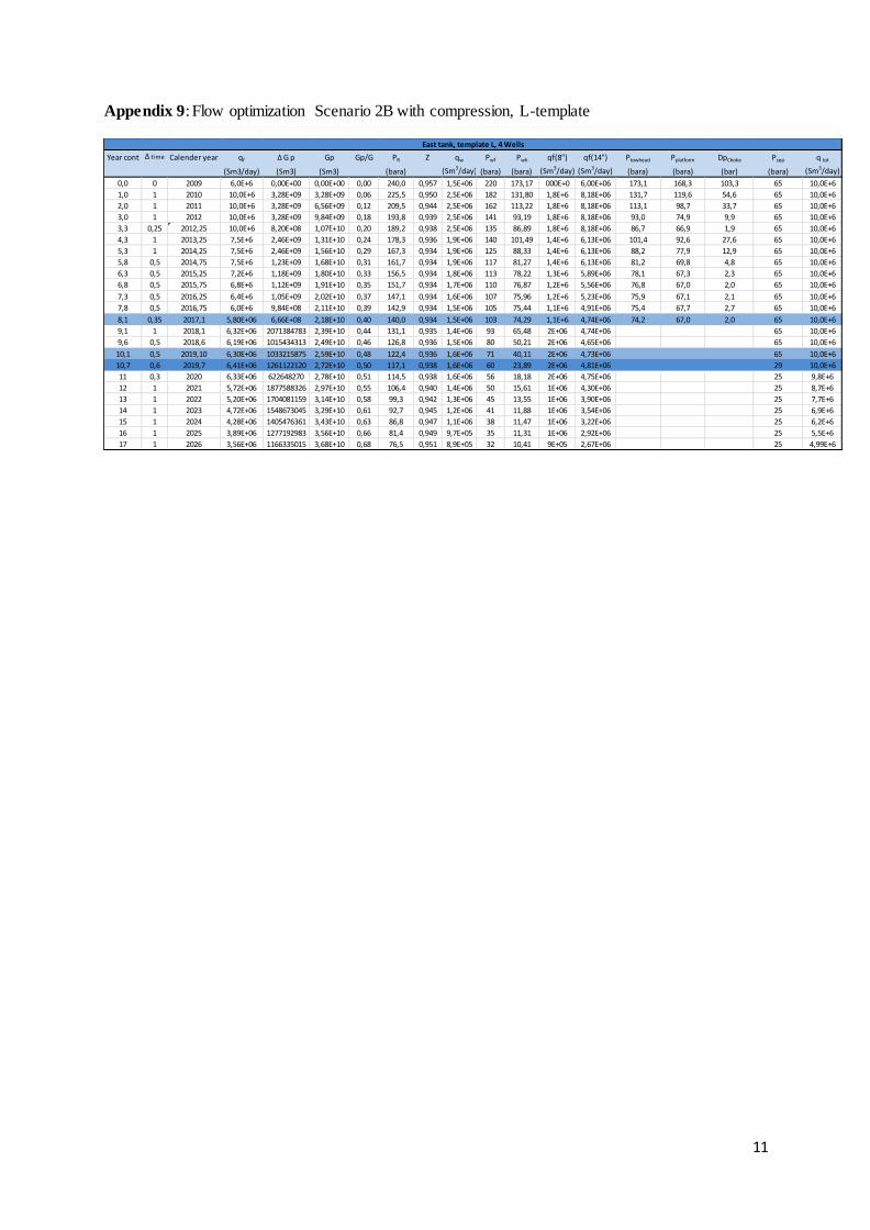
11
Appendix 9: Flow optimization Scenario 2B with compression, L-template
Year cont ∆ time Calender year qf ∆ G p Gp Gp/G PR Z qw Pwf Pwh qf(8") qf(14") Ptowhead Pplatform DpChoke Psep q tot
(Sm3/day) (Sm3) (Sm3) (bara) (Sm3/day) (bara) (bara) (Sm3/day) (Sm3/day) (bara) (bara) (bar) (bara) (Sm3/day)
0,0 0 2009 6,0E+6 0,00E+00 0,00E+00 0,00 240,0 0,957 1,5E+06 220 173,17 000E+0 6,00E+06 173,1 168,3 103,3 65 10,0E+6
1,0 1 2010 10,0E+6 3,28E+09 3,28E+09 0,06 225,5 0,950 2,5E+06 182 131,80 1,8E+6 8,18E+06 131,7 119,6 54,6 65 10,0E+6
2,0 1 2011 10,0E+6 3,28E+09 6,56E+09 0,12 209,5 0,944 2,5E+06 162 113,22 1,8E+6 8,18E+06 113,1 98,7 33,7 65 10,0E+6
3,0 1 2012 10,0E+6 3,28E+09 9,84E+09 0,18 193,8 0,939 2,5E+06 141 93,19 1,8E+6 8,18E+06 93,0 74,9 9,9 65 10,0E+6
3,3 0,25 2012,25 10,0E+6 8,20E+08 1,07E+10 0,20 189,2 0,938 2,5E+06 135 86,89 1,8E+6 8,18E+06 86,7 66,9 1,9 65 10,0E+6
4,3 1 2013,25 7,5E+6 2,46E+09 1,31E+10 0,24 178,3 0,936 1,9E+06 140 101,49 1,4E+6 6,13E+06 101,4 92,6 27,6 65 10,0E+6
5,3 1 2014,25 7,5E+6 2,46E+09 1,56E+10 0,29 167,3 0,934 1,9E+06 125 88,33 1,4E+6 6,13E+06 88,2 77,9 12,9 65 10,0E+6
5,8 0,5 2014,75 7,5E+6 1,23E+09 1,68E+10 0,31 161,7 0,934 1,9E+06 117 81,27 1,4E+6 6,13E+06 81,2 69,8 4,8 65 10,0E+6
6,3 0,5 2015,25 7,2E+6 1,18E+09 1,80E+10 0,33 156,5 0,934 1,8E+06 113 78,22 1,3E+6 5,89E+06 78,1 67,3 2,3 65 10,0E+6
6,8 0,5 2015,75 6,8E+6 1,12E+09 1,91E+10 0,35 151,7 0,934 1,7E+06 110 76,87 1,2E+6 5,56E+06 76,8 67,0 2,0 65 10,0E+6
7,3 0,5 2016,25 6,4E+6 1,05E+09 2,02E+10 0,37 147,1 0,934 1,6E+06 107 75,96 1,2E+6 5,23E+06 75,9 67,1 2,1 65 10,0E+6
7,8 0,5 2016,75 6,0E+6 9,84E+08 2,11E+10 0,39 142,9 0,934 1,5E+06 105 75,44 1,1E+6 4,91E+06 75,4 67,7 2,7 65 10,0E+6
8,1 0,35 2017,1 5,80E+06 6,66E+08 2,18E+10 0,40 140,0 0,934 1,5E+06 103 74,29 1,1E+6 4,74E+06 74,2 67,0 2,0 65 10,0E+6
9,1 1 2018,1 6,32E+06 2071384783 2,39E+10 0,44 131,1 0,935 1,4E+06 93 65,48 2E+06 4,74E+06 65 10,0E+6
9,6 0,5 2018,6 6,19E+06 1015434313 2,49E+10 0,46 126,8 0,936 1,5E+06 80 50,21 2E+06 4,65E+06 65 10,0E+6
10,1 0,5 2019,10 6,30E+06 1033215875 2,59E+10 0,48 122,4 0,936 1,6E+06 71 40,11 2E+06 4,73E+06 65 10,0E+6
10,7 0,6 2019,7 6,41E+06 1261122120 2,72E+10 0,50 117,1 0,938 1,6E+06 60 23,89 2E+06 4,81E+06 29 10,0E+6
11 0,3 2020 6,33E+06 622648270 2,78E+10 0,51 114,5 0,938 1,6E+06 56 18,18 2E+06 4,75E+06 25 9,8E+6
12 1 2021 5,72E+06 1877588326 2,97E+10 0,55 106,4 0,940 1,4E+06 50 15,61 1E+06 4,30E+06 25 8,7E+6
13 1 2022 5,20E+06 1704081159 3,14E+10 0,58 99,3 0,942 1,3E+06 45 13,55 1E+06 3,90E+06 25 7,7E+6
14 1 2023 4,72E+06 1548673045 3,29E+10 0,61 92,7 0,945 1,2E+06 41 11,88 1E+06 3,54E+06 25 6,9E+6
15 1 2024 4,28E+06 1405476361 3,43E+10 0,63 86,8 0,947 1,1E+06 38 11,47 1E+06 3,22E+06 25 6,2E+6
16 1 2025 3,89E+06 1277192983 3,56E+10 0,66 81,4 0,949 9,7E+05 35 11,31 1E+06 2,92E+06 25 5,5E+6
17 1 2026 3,56E+06 1166335015 3,68E+10 0,68 76,5 0,951 8,9E+05 32 10,41 9E+05 2,67E+06 25 4,99E+6
East tank, template L, 4 Wells