submitted to International Journal of Computer Vision June, 2002

The Dual-Bootstrap Iterative Closest Point Algorithm with

Application to Retinal Image Registration

Charles V. Stewart1 Chia-Ling Tsai1 Badrinath Roysam2

1Dept. of Computer ScienceRensselaer Polytechnic Institute

Troy, New York 12180–3590stewart,tsaic@cs.rpi.edu

2Dept. of Electrical, Computer,and

Systems EngineeringRensselaer Polytechnic Institute

Troy, New York 12180–3590roysab@rpi.edu

June 24, 2002

Abstract

A new generalization of the Iterative Closest Point (ICP) registration algorithm is introducedand incorporated into a complete algorithm for registering retinal images. ICP works by iteratingtwo steps: matching points based on the current transformation estimate and refining the esti-mate based on the matches. It requires a good initial estimate. By contrast, the Dual-BootstrapICP algorithm only requires an initial estimate that is a “toe hold” on the correct alignment —accurate only locally, over a small image region, and perhaps using a lower-order transformationthan is needed to accurately align the entire images. The algorithm iteratively “bootstraps” boththe region over which the model is accurate and the chosen transformation model, using a robustversion of standard ICP restricted to the bootstrap region during each iteration. The covarianceof the transformation estimate controls both bootstrap processes. The algorithm is designed tohandle several difficult circumstances in registration: (a) data from which relatively poor initialestimates can be reliably obtained, (b) data that has structural (geometric) complexity such asmultiple proximate curves and surfaces, (c) data that has many missing or extraneous points,and (d) image pairs that have low overlap. In registering retinal image pairs, the Dual-BootstrapICP algorithm is initialized from similarity transformation estimates obtained by matching in-dividual or pairs of vascular landmarks, and it aligns images based on blood vessel centerlinesto produce quadratic transformations. On tests involving approximately 6000 image pairs, itsuccessfully registered 99.5% of the pairs containing at least one common landmark, and 100%of the pairs containing at least one common landmark and 35% overlap or higher. This nearflawless performance enables a variety of applications.

RPI-CS-TR 02-9 2

Index terms: Registration, iterative closest point, robust estimation, retinal imaging

RPI-CS-TR 02-9 1

1 Introduction

1.1 The Iterative Closest Point Algorithm

The iterative closest point (ICP) registration algorithm was invented almost simultaneously

in the early 1990’s by several different research groups [3, 12, 14, 49, 78], and has been used

in many different applications since then [22, 43, 49, 55]. ICP is a point-based registration

algorithm, where the “points” may be raw measurements such as (x, y, z) values from range

images, intensity points in three-dimensional medical images [24, 29], and edge elements, corners

and interest points [64] that locally summarize the geometric structure of the data. ICP should

be used when correspondences between the point sets are not known and when matching based

on the properties of individual points (and their surroundings) does not produce a large enough

set of unique correspondences to precisely align the two data sets.

To fix the idea of the ICP algorithm, let I1 and I2 denote the two data sets and let θ be the

parameter vector of the transformation mapping the coordinate system of I1 onto the coordinate

system of I2. ICP iterates two main steps: (1) using a fixed estimate, θ̂, the transformation

is applied to each point from image dataset I1 and the closest point in image dataset I2 is

found as a temporary match, and (2) using constraints formed from these matches, a new best

estimate θ̂ is computed. (In some cases, matches are only formed implicitly [12].) This process

is repeated until the estimate θ̂ stabilizes. Different instantiations of the ICP algorithm use

different combinations of image points, distance metrics, and transformation models. These affect

convergence rates and accuracy, but not the general structure of the algorithm. Clearly, as an

iterative minimization algorithm, ICP requires proper initialization, and a variety of techniques

may be used: application specific constraints [54, 55], image-wide measures on the data sets such

as statistical moments and geometric attributes [35, 38], multiresolution methods [24], and initial

matching of distinctive features [16, 19, 67, 74].

The literature on ICP has concentrated on initialization, efficient matching [1, 60], and ap-

plications, while leaving the algorithmic structure unchanged. The motivating observation of

this paper is different, however: there are situations where initial estimates alone are not enough

to ensure that ICP will convergence to an accurate transformation estimate. We illustrate the

problem in the context of registering images of the human retina and then consider general prop-

erties of the problem. Figure 1 shows two different images of the same retina taken at the same

RPI-CS-TR 02-9 2

time. The viewpoint of the images is somewhat different, and different regions of the retina are

well-focused in the images. The features used in registration are the branching and cross-over

points of the vasculature (seen in Figure 1(a) and (b)) and the centerline points of the vasculature

(Figure 1(c) and (d)). The former are used for initialization of ICP, whereas the latter are used

in the iterative steps of ICP. In this case, only the landmark circled in (a) and (b) is in common

between the two images. Computing an initial similarity transformation based on aligning this

landmark and the surrounding vasculature yields the alignment shown in Figure 2(a). Starting a

robust version of ICP algorithm from this initial estimate and letting it converge yields the incor-

rect result shown in Figure 2(b). This is based on using a similarity transformation throughout

and then switching at the end to a quadratic transformation [11] that accounts for the curvature

of the retina. If instead the quadratic transformation is used immediately, a similar incorrect

result is obtained.

This example illustrates a general problem with ICP algorithms — convergence to an incor-

rect final registration starting from an initial estimate that locally appears correct. Since ICP

algorithms have been used successfully in a variety of applications, it is important to outline the

circumstances under which this problem can arise. An intuitive discussion is given here, with a

technical analysis saved for later in the paper. The problem can arise under a combination of

the following four circumstances:1

Geometric data complexity: Repetitive structures such as meshes, multiple elongated struc-

tures such as blood vessels and nerve fibers, and high-frequency structure such as in brain

images create many opportunities for mismatches when there are even small misalignments.

Such complexity raises the level of accuracy required in the initial estimate.

Data quality: Low data quality means that points and even whole structures (e.g. individual

blood vessels) can appear in one image, but be missing in another. (For the images in

Figure 1, within the region that is common between the images only 63% of the center-

line points are in common; image-wide this drops to 58%.) These “outliers” can cause

mismatches that skew the parameter estimates, converting small misalignments into much

larger ones.1We are ignoring for this paper the difficulties of multimodal registration where different imaging modalities

make completely different structures — bone vs. soft tissue — prominent [22].

RPI-CS-TR 02-9 3

(a) (b)

(c) (d)

Figure 1: Illustrating retinal fundus images of an unhealthy eye (nonexudative age-related mac-ular degeneration) together with image features used in ICP registration. Panels (a) and (b)show the images, with landmarks extracted by our retinal image tracing algorithm [8, 27]. Thelandmarks are branching and cross-over points of the retinal vasculature. These are used ininitializing ICP. Panels (c) and (d) show the centerline points obtained by the tracing algorithmand used in the iterative steps of ICP. Many inconsistencies in the two sets of traces may beobserved.

Low overlap: Low overlap can cause similar problems to low-quality data, except that there

is coherence to what’s missing — entire image regions. Low overlap is challenging for

initialization based on image-wide measures and on multiresolution methods. Moreover, it

raises the level of significance of each constraint used in registration, implying that more

accuracy is required of each.

High-order transformation models: These require more constraints to initialize and can

introduce greater distortions in the data sets. In the example shown, a 12-parameter,

RPI-CS-TR 02-9 4

(a) (b)

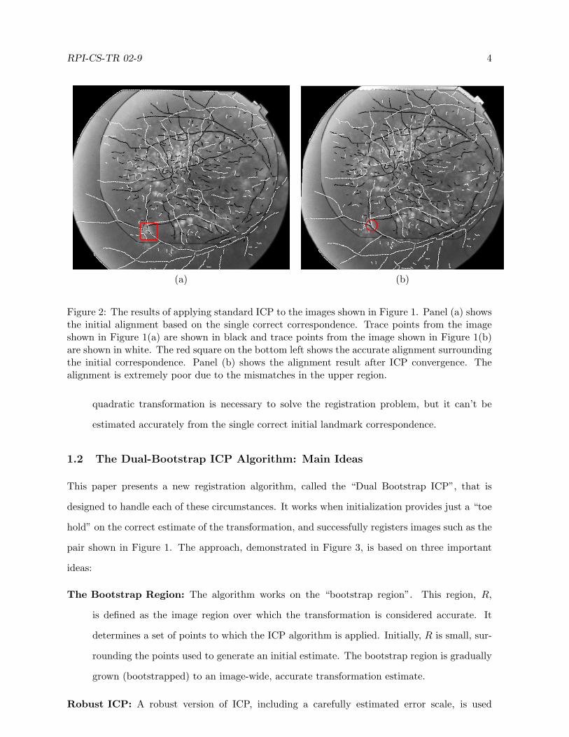
Figure 2: The results of applying standard ICP to the images shown in Figure 1. Panel (a) showsthe initial alignment based on the single correct correspondence. Trace points from the imageshown in Figure 1(a) are shown in black and trace points from the image shown in Figure 1(b)are shown in white. The red square on the bottom left shows the accurate alignment surroundingthe initial correspondence. Panel (b) shows the alignment result after ICP convergence. Thealignment is extremely poor due to the mismatches in the upper region.

quadratic transformation is necessary to solve the registration problem, but it can’t be

estimated accurately from the single correct initial landmark correspondence.

1.2 The Dual-Bootstrap ICP Algorithm: Main Ideas

This paper presents a new registration algorithm, called the “Dual Bootstrap ICP”, that is

designed to handle each of these circumstances. It works when initialization provides just a “toe

hold” on the correct estimate of the transformation, and successfully registers images such as the

pair shown in Figure 1. The approach, demonstrated in Figure 3, is based on three important

ideas:

The Bootstrap Region: The algorithm works on the “bootstrap region”. This region, R,

is defined as the image region over which the transformation is considered accurate. It

determines a set of points to which the ICP algorithm is applied. Initially, R is small, sur-

rounding the points used to generate an initial estimate. The bootstrap region is gradually

grown (bootstrapped) to an image-wide, accurate transformation estimate.

Robust ICP: A robust version of ICP, including a carefully estimated error scale, is used

RPI-CS-TR 02-9 5

throughout the bootstrapping process to avoid skewed estimates due to mismatches.

Bootstrapping the Model: Rather than using a single, fixed transformation model, different

models are used in different bootstrap regions, starting from a simple model for the initial

bootstrap region and gradually evolving to a higher-order model as the bootstrap region

grows to describe the entire data set. Model selection techniques [7, 75], which depend

fundamentally on the parameter estimate covariance matrix, are used to automatically

select the transformation model for each bootstrap region.

Thus, the term “dual-bootstrap” refers to simultaneous growth in the bootstrap region and the

transformation model order. It is applied to one or more initial bootstrap regions independently,

ending with success when one bootstrap region R is expanded to a sufficiently-accurate, image-

wide transformation.

1.3 Retinal Image Registration

The Dual-Bootstrap ICP algorithm is described as a general technique, but then applied to

retinal image registration. This is an important application and, as shown above, illustrates the

major difficulties of ICP registration. Registering retinal images taken at different times — with

time gaps ranging from minutes, to hours, to days, to a year or more — can form the basis for

measuring (a) the effect of surgery [25, 40, 61, 69], (b) the progress of diseases [34, 41, 42, 48],

and (c) the impact of drugs and nutritional supplements [20, 28, 52]. Retinal image registration

can also be used for montaging images to obtain a complete view of the retina, and to integrate

ordinary retinal fundus images with angiograms showing blood flow in both the retinal and

choroidal vasculature [18, 73].

2 Robust ICP Problem Formulation

We start by presenting a mathematical problem formulation for point-based registration algo-

rithms. This will provide a formal context for the main contributions of the Dual-Bootstrap ICP

algorithm. One difference between this formulation and standard versions is the use of robust

estimation [31, 59, 70].

The formulation starts with two sets of point vectors, P = {pi} from image I1 and Q = {qj}

RPI-CS-TR 02-9 6

(a) (b)

(c) (d)

(e)

Figure 3: Illustrating the Dual Bootstrap ICP algorithm in retinal image registration using theimages and feature points shown in Figure 1 and the initial alignment shown in Figure 2. Ineach iteration, a robust version of ICP is applied only in the bootstrap region, Rt, indicatedby the red rectangle in each figure. The transformation is only required to be accurate in thisbootstrap region. Also in each iteration, the best transformation model (in this case, similarity,reduced-quadratic, or quadratic — see Table 1) is automatically selected and the bootstrapregion is grown. Several increments of this process are shown in the panels, and the modelselected in each bootstrapping iteration is indicated. Panel (e) shows the final alignment usinga 12-parameter quadratic model.

RPI-CS-TR 02-9 7

from image I2. These points could be as simple as (x, y, z)T coordinates taken from range images,

or they could be descriptions of edge elements, interest points [64, 68], corner locations [32], or

other image structures. The problem is to find the transformation parameters, θ, and associated

set of correspondences, C ⊂ P × Q, that minimize an appropriate error distance. A general

objective function to be minimized can be written as

E(θ, σ; C) =∑

(pi,qj)∈C

ρ(d(M(θ; pi),qj)/σ). (1)

The components of this objective function are described as follows:

• M(θ; pi) is the mapping of pi into the coordinate system of I2 based on transformation

parameter vector θ. A common and simple case of this mapping is a rigid transformation

of a point coordinate vector from <n to <n. The mapping may be more general and it

may be extended to apply to tangent vectors, normal vectors, and other geometric or even

photometric properties [23, 39].

• d(M(θ; pi),qj) is a distance metric in the coordinate system of I2 between the mapped

vector and the corresponding vector qj .2 The distance metric depends on the types of point

vectors. For detected corner points, interest points or other image landmarks, the natural

metric is the Euclidean distance. For points that are samples from smooth regions of curves

or surfaces, point-to-line or point-to-plane normal distances are generally more appropriate

[3, 14]. These alternatives are illustrated using an example in Figure 4. Algebraically, if

η̂j is the line (2d) or plane (3d) normal, then the normal distance is

d(M(θ; pi),qj) = |(M(θ; pi)− qj)T η̂j |.

Combinations of constraints are also possible.

• ρ(u) is a robust loss function [31, 59, 70], monotonically non-decreasing as a function of |u|.

A least-squares loss function is obtained by making ρ(u) = u2, but because mismatches

are common, robust loss functions, which down-grade the significance of mismatches, are

crucial [31, 59, 70]. See Figure 5 for plots of example functions.2See [33, Ch. 3] for formulations where error distances are measured in both images. These more complicated

minimization problems are beyond the scope of our discussion.

RPI-CS-TR 02-9 8

Matched landmarks

trace points

I I1 2

Current transformation

Matched

Figure 4: A schematic illustrating distance metrics on landmarks and on trace centerpoints. Theregion around a vascular landmark is shown in I1, including the landmark location itself and aseparate trace point. These are mapped onto I2 using the current transformation and matchedagainst the landmark location and trace points. The landmark location match should generatea Euclidean distance constraint, whereas the trace point match, which is in fact mismatchedslightly, should generate constraint that measures point-to-line distance. The line is the local,linear approximation to the contour, with tangent vectors shown.

0

2

4

6

8

10

12

14

-6 -4 -2 0 2 4 6

Least-squaresCauchy

Beaton-Tukey

0

0.2

0.4

0.6

0.8

1

1.2

-6 -4 -2 0 2 4 6

Least-squaresCauchy

Beaton-Tukey

(a) (b)

Figure 5: Plots of the robust loss function ρ(u) (a) and weight function w(u) = ρ′(u)/u (b)for the Beaton-Tukey biweight loss function, the Cauchy loss function and the quadratic lossfunction, which equates to least-squares estimation. The weight function is used in the itera-tively reweighted least-squares implementation of M-estimators [36]. The Beaton-Tukey is chosenbecause it most aggressively rejects outliers, providing no weight to matches with normalized dis-tances greater than about 4 standard deviations.

• σ is the error scale, which is the (robust) standard deviation of the error distances. This

must be estimated carefully: when the estimate σ̂ is too small correct correspondences may

be treated as outliers, but when σ̂ is too large mismatches may be treated as inliers. Either

case causes bias in the transformation estimate. A different issue is that as written, the

RPI-CS-TR 02-9 9

objective function shown in ( 1) is minimized by σ → ∞. This can be avoided by adding

a log(σ) term [37] or by (robustly) estimating and then fixing σ using a separate process

during minimization [70].

• To avoid the trivial minimum corresponding to C = {}, restrictions are often placed on C. A

common one is to make P a subset of the points from I1 and require a single correspondence

in C for each p ∈ P. We will make this assumption throughout the paper.

Various instantiations of the ICP algorithm differ primarily in the type of data, and the

choices of mapping function and distance metric. They also differ in the data representations

and matching techniques, but mainly these are implementation details. Once these are specified

and the data sets and initial value of θ are provided, ICP is straightforward. It simply works

by alternately fixing θ and estimating C and then fixing C and estimating θ, repeating until

convergence. Multiple starting points may be provided and the ICP algorithm may be embedded

in a multiresolution hierarchy, but our primary concern is the algorithm itself. Once substantial

improvements are made, the new algorithm can be combined with a variety of initialization

techniques. The improvements made will allow convergence to a desirable estimate from weaker

initial conditions, reducing the significance of initialization.

3 The Dual-Bootstrap ICP Algorithm

The improvements of the Dual-Bootstrap ICP algorithm are obtained through manipulating the

structure of the objective function (1) during minimization. The final minimization is the same

however. This manipulation is done in two ways:

• The image I1 point set P is not treated as fixed. Instead, it is dictated by the bootstrap

region, R, which starts as a small, compact subset of the image I1 data and eventually

grows to encompass the entire portion of I1 that overlaps I2. We denote the sequence of

regions by (R1, . . . , Rt, . . .) where the subscript t indicates the iteration number, and write

the point set as Pt = P(Rt) to indicate the region dependency.

• A set of transformation models M and associated parameter vectors θ is used, not just

a single model. We denote the model set by {M1, . . . ,Mf} and the sets of associated

parameter vectors by {θ1, . . . ,θf}. One of these models is automatically selected for each

RPI-CS-TR 02-9 10

bootstrap region, Rt. The set of models may or may not form a nested hierarchy. The

model set is needed when the data from which the estimates are initialized does not provide

enough information for a reliable estimate of the parameters of the full model. (A restricted

form of the Dual-Bootstrap ICP algorithm can be used with only a single model.) Let Mmt

denote the model selected at iteration t for region Rt, and let θ̂mt denotes the associated

estimate of the model parameter vector.

Thus, at each iteration of the Dual-Bootstrap ICP algorithm, a 6-tuple is determined:

(Rt,Pt, Ct,Mmt , θ̂mt , σ̂t).

As the algorithm converges, Rt should stabilize on the portion of I1 overlapping I2, Ct should be

a correct set of correspondences for this region, Mmt should be the full model, and θ̂mt and σ̂t

should approach the correct model and scale parameters.

3.1 Algorithm Outline

The outline of the actual algorithm is straightforward given the above discussion. It is again

important to note that the Dual-Bootstrap ICP algorithm is an iterative minimization technique

and therefore procedures outside the algorithm should provide the starting estimate. Thus, the

following description is based on a single starting estimate.

1. Establish the initial bootstrap region R1 in a small area around where the initial estimate

is computed, and initialize model Mm1 to be the lowest order model.

2. t = 1;

3. While the estimate has not converged

(a) Select the points Pt from Rt.

(b) Apply robust ICP to determine the correspondence set, Ct, the transformation esti-

mate θ̂mt , and the scale estimate σ̂t. Calculate the covariance matrix, Σmt , of the

estimate.

(c) Bootstrap the model: using the correspondence set, Ct, and the covariance matrix Σmt ,

apply a model selection technique to choose the new model Mmt+1 . If Mmt 6= Mmt+1 ,

RPI-CS-TR 02-9 11

calculate a new covariance matrix.

(d) Bootstrap the region: Use the covariance matrix, Σmt , and the new model Mmt+1

to expand the region based on the covariance propagation error. The growth rate is

inversely related to the error.

(e) Check for convergence. The algorithm will converge just like normal ICP after the

bootstrap region, Rt, stabilizes.

(f) t = t+ 1

Details are described in the following subsections.

3.2 Bootstrap Regions

For simplicity, the bootstrap regions Rt are rectangular. Other region shapes may be used

without affecting the structure of the algorithm.

3.3 Covariance and Transfer Error

The covariance matrix of the parameter vector estimate [71] is needed in both model selection and

region growth. The parameter estimate is denoted by θ̂. The covariance matrix is approximated

by the inverse Hessian of E(θ̂)

Σmt = H−1(E(θ̂mt)). (2)

Here, E(·) is as defined in Equation 1, with the correspondence set Ct fixed. Hence, the inverse

Hessian is computed just with respect to the model parameter vector. There is no need to scale

the inverse Hessian by the error variance because the error variance is included in the objective

function.

The formation of the matching constraints plays an important role in (2). These constraints

must realistically describe the information that is truly provided by a correspondence. To take

an extreme and somewhat unrealistic example, suppose the points pi are sampled from a single,

infinite line in image I1 and matched to a corresponding infinite line in I2. Let the corresponding

points found by ICP on the line be qi, and suppose just rotation and translation are being

estimated. Then, if Euclidean distance constraints are used in (1), the covariance matrix will

appear to be extremely stable, whereas if normal distance constraints (Section 2) are used, the

RPI-CS-TR 02-9 12

covariance matrix will be unstable. Clearly, the latter is correct because translation along the

line is undetermined. This is the aperture problem in registration.

The Dual-Bootstrap ICP algorithm uses Σmt in bootstrapping the model, and in bootstrap-

ping the region. In the latter, Σmt is applied to calculate the transfer uncertainty in mapping a

point from I1 to I2 [33, Ch. 4]. Let point p be an image location in I1 and let p′ = Mmt(θ̂mt ; p)

be the transformed location in I2. Computing the covariance of p′ requires the Jacobian of the

transformation:

J(p) =∂M(θ̂mt ; p)

∂p.

Combining this with Σmt gives the covariance of the transformed point:

Σp′ = J(p) Σmt J(p)T . (3)

This equation may be generalized as required when the points are more than just coordinate

locations.

3.4 Robust ICP

A robust version of the standard ICP algorithm is used as part of the Dual Bootstrap ICP

algorithm. Recall that standard ICP alternates steps of matching and parameter estimation.

The main innovations here are in robust parameter estimation and especially in error scale

estimation.

In matching, the standard ICP technique is to find the closest feature point to p′ = Mmt(θ̂mt ; p),

where p is one of the feature points in Pt selected from Rt. A variety of techniques, such as digital

distance maps [6, 21] in 2D, octree splines [72] and z-buffering [1], may be used to accelerate this

process [3, 60]. All of the matches are placed in the correspondence set Ct for this iteration.

Given Ct, the new estimate of the transformation parameters θ̂mt is computed by minimizing

Et(θmt) =∑

(p,q)∈Ct

ρ(d(Mmt(θmt ; p),q)/σ̂). (4)

As discussed earlier, ρ is a robust “loss” function. Three robust loss functions are illustrated in

Figure 5. Equation 4 may be solved using iteratively-reweighted least-squares (IRLS) [36], with

weight function w(u) = ρ′(u)/u. The minimization process alternates weight recalculation using

RPI-CS-TR 02-9 13

a fixed parameter estimate with weighted least-squares estimation of the parameters. Levenberg-

Marquardt techniques may also be used to minimize Et(·).

The choice of loss functions is motivated by looking at the associated weight functions illus-

trated in Figure 5. The least-squares loss function has a constant weight, the Cauchy weight

function descends and asymptotes at 0, while the Beaton-Tukey biweight function has a hard

limit beyond which the weight is 0. The latter is important for rejecting errors due to mismatches.

The details of the Beaton-Tukey biweight are

ρ(u) =

a2

6

[1− (1−

(ua

)2)3] |u| ≤ aa2

6 |u| > a

and

w(u) =

[1−

(ua

)2]2 |u| ≤ a

0 |u| > a.

Using, a ≈ 4.0 [36], means that correspondences producing errors larger than about 4 error

standard deviations have no weight. Other loss functions sharing this hard-limit property could

also be used.

This discussion shows why accurately estimating the error scale, σ, is crucial. Estimation of

error scale is done for each set of correspondences at the start of reweighted least-squares. We use

a technique called MUSE that automatically adjusts its estimate by determining the fraction of

(approximately) correct matches [50, 51]. This is important because sometimes more than 50%

of the feature points in Rt are mismatched. (An example of this occurs during the registration

process shown in Figure 3 when Rt covers about half the overlap between images.) Let rj =

|d(Mmt(θ̂mt ; p),q)| be the absolute error estimate for the jth correspondence using the current

estimate θ̂mt of the transformation parameters. Let r1:N , r2:N , . . . , rN :N be a rearrangement of

these values into non-decreasing order. Then for any k, r1:N , . . . , rk:N are the k smallest errors.

A scale estimate may be generated from r1:N , . . . , rk:N as

σ2k =

∑kj=1 r

2j:N

C(k,N),

where C(k,N) is a computed correction factor. This factor makes σ2k an unbiased estimate of

RPI-CS-TR 02-9 14

the variance of a normal distribution using only the first k out of N errors. The intuition behind

MUSE is seen by considering the effect of outliers on σ2k. When when k is large enough to start

to include outliers (errors from incorrect matches), values of σ2k starts to increase substantially.

When k is small enough to include only inliers, σ2k is small and approximately constant. Thus,

we can simply evaluate σ2k for a range of values of k (e.g. 0.35N, 0.40N, . . . 0.95N), and choose

the smallest σ2k. To avoid values of k that are too small, we in fact take the minimum variance

value of σ2k, not just the smallest σ2

k. Details are in [50, Chapter 3].

3.5 Bootstrapping the Model

Increasing complexity models can and should be used as the bootstrap region, Rt, increases in

size and includes more constraints. Changing the model order must be done carefully, however.

Switching to higher order models too soon causes the estimate to be distorted by noise. Switching

too late causes modeling error to increase the error scale, σ̂, and causes misalignments on the

boundaries of Rt. Both of these cause mismatching. An example of the latter is shown in Figure 6.

To select the correct model for each bootstrap region, statistical model selection techniques are

applied.

Automatic model selection is a well-studied problem [7, 75], and experimental analysis shows

that none of the techniques is ideal [7]. All techniques choose the model that optimizes a trade-off

between the fitting accuracy of high-order models and the stability of low-order models. The

current Dual-Bootstrap ICP model selection criteria is adapted from [7]. The expression is

dm2

log 2π −∑i

wir2i + log det(Σθ), (5)

where dm is the degrees of freedom in the model,∑

iwir2i is the sum of the robustly-weighted

transformation errors, and det(Σθ) is the determinant of the parameter estimate covariance

matrix. Notice that if Σθ is not full-rank, then the third term goes to −∞.

In the model bootstrap step of the Dual-Bootstrap ICP algorithm, expression (5) is evaluated

for each model, M1, . . . ,Mf , using the fixed set of matches Ct determined by robust ICP in

iteration t. For each model, iteratively-reweighted least-squares estimation is applied, and the

final weights, error residuals, and computed covariance matrix are used to evaluate (5). The

model yielding the largest value is taken as the new model, Mmt+1 .

RPI-CS-TR 02-9 15

One step that could be added is to allow rematching with different models prior to model

selection — in other words to run full robust ICP for each model. If there is a smooth transition

between models, which means that the switch in models in a fixed bootstrap region, Rt, does not

dramatically change the mapped locations of points in Rt, then this is unlikely to be necessary.

This issue is discussed further in Section 6.

The final issue in bootstrapping the model is that an appropriate set of models must be

chosen. This is an application-specific consideration, but two concerns must be addressed. First,

the models should be based on geometrically-plausible approximations to the image-wide trans-

formation. Otherwise, the added degrees of freedom can lead to improper distortions of the

transformation in response to mismatches and noise. Second, there should be a gradual increase

in the precision of the models as applied in the given application. Otherwise, the algorithm may

stay with a lower-order model too long (Figure 6) or switch to a higher-order model too early.

(a) (b)

Figure 6: An example using retinal image registration showing an example of mismatching at theborder of the region if the change in model order occurs too late. In (a) a similarity transformationis used for a large bootstrap region, and the vascular structure on the left border (indicated bythe arrow) is mismatched. (Matches are shown by the yellow line segments.) As seen in (b)this eventually causes convergence to the incorrect final transformation estimate. In our actualimplementation this mistake does not happen because bootstrap model selection switches to ahigher-order model before Rt grows to include this area of the image.

3.6 Bootstrapping the Region – Region Expansion

The bootstrap region is expanded based on transfer error (Section 3.3) for points on the bound-

ary of Rt, with lower transfer error leading to faster bootstrap region growth. In the current

RPI-CS-TR 02-9 16

algorithm, region Rt is rectangular. Each side of Rt is expanded independently, allowing more

rapid expansion where there is less ambiguity (see Figure 3). For each segment, let u be the

point in the center of the segment that defines the side (see Figure 7 for a depiction of Rt for

two-dimensional images), let d be the outward normal at u, let u′ be the transformed location

of u based on the current model and estimate, and let Σu′ be the covariance matrix for this

point (Equation 3). Note that all of these estimates are computed in a coordinate system that is

aligned with the center of Rt. The uncertainty of the transformation of u in outward direction

d, is

U(u,d) = max(1,dTΣu′d).

The change in location u is (|uTd|βU(u,d)

)d.

Here, β determines the maximum expansion rate at each side. The lower bound of 1 in U(u,d)

prevents region growth that is too rapid. Clearly, as U(u,d) → ∞, the expansion of u goes to

0. The new region Rt+1 is the rectangle (in two-dimensions) formed by the expanded sides. The

growth parameter β is set based on the desired maximum growth rate. For example, setting β

to√

2− 1 ensures that Rt does no more than double in area in each iteration.

dt = (0,1)

d = (−1,0)l

ub

ul

db

dr= (1,0)

= (0,−1)

ut

ur

expansion direction

expansion point

center of the region

Figure 7: The bootstrap region is expanded by moving out perpendicular to each side. Indirections where the estimate is more stable, expansion is faster.

RPI-CS-TR 02-9 17

4 Retinal Image Registration Using Dual-Bootstrap ICP

A major consequence of the sophisticated minimization technique of the Dual-Bootstrap ICP

algorithm is that the initial conditions from which it can converge are substantially weakened.

We have described it as requiring just a “toe hold” on an accurate alignment. This means that

the initial estimate must be accurate enough to generate (mostly) correct correspondences in the

bootstrap region in the first iteration.

For retinal image registration, this is crucial. In high-quality images of healthy retinas,

many landmarks are available to initialize matching. In lower quality images or in images of

unhealthy retinas, fewer landmarks are prominent. Therefore, we implement the Dual-Bootstrap

ICP algorithm in retina image registration to start from a similarity transformation initialized

by matching a single pair of landmarks or by matching two pairs of landmarks. The algorithm

tests many different initial correspondences, allowing the Dual-Bootstrap ICP to converge for

each. It stops and accepts as correct a registration having a stable transformation and a highly

accurate alignment. As we will see, the complete algorithm has nearly flawless performance.

Here are some of the important implementation details:

Point sets: As discussed earlier, the points (Figure 1) are the blood vessel centerlines and land-

marks — branches and cross-over points of blood vessels — extracted using an exploratory

algorithm described in [8, 66, 27]. The centerline points are characterized by location,

orientation and width, while the landmarks are characterized by their center location, the

orientation of the blood vessels that meet to form them, and the widths of these vessels

(Figure 8).

Invariants: Matches between two landmarks, one in each image, or between pairs of landmarks

in each image are generated by computing and comparing invariants [4, 53]. Invariants for

a single landmark are blood vessel width ratios and blood vessel orientations (Figure 8),

giving a five-component invariant signature vector. The invariant signature of a set of

two landmarks is a six-component vector (Figure 9). The line segment drawn between the

two landmarks forms an axis, and the orientation of each of the three landmark angles is

computed with respect to this axis, giving the six components. The combination of two

types of invariant is used because the single-landmark invariants are the limit of what can

RPI-CS-TR 02-9 18

be accomplished by matching landmarks, whereas the pair-invariants allow more flexibility

to changes in orientation and mismeasurement of blood-vessel width.

Figure 8: A landmark is characterized by a center location qc, the orientations φj of the threeblood vessels that meet to form it and the widths wj of the blood vessel. The traced vascularcenterline points are illustrated by the small, hollow circles on the leftmost vessel. Differences inorientations and the ratios of the blood vessel widths are invariant to rotation, translation andscaling of the image — a similarity transformation. The orientations themselves are invariant totranslation and scaling.

Figure 9: The invariant signature of a pair of landmarks. The line segment drawn betweenthe two landmarks forms an axis, and the orientation of each of the three landmark angles iscomputed with respect to this axis, giving a six-component signature vector.

Initial matching: The invariant signature vectors for one- and two-landmark sets are computed

separately for each image, I1 and I2, and then matched (each set separately). At least

one match is found for each signature vector. Additional matches are determined when

the Mahalanobis distance between signature vectors is within a chi-squared uncertainty

bound. Each signature match produces a set of one or two landmark correspondences.

These sets are ordered for testing by chi-squared confidence levels. For each set, a similarity

RPI-CS-TR 02-9 19

transformation is computed which generates the initial transformation.

Iterative matching: The matching constraints during iterative minimization of Dual-Bootstrap

ICP are point-to-line matches (illustrated in Figure 4). To facilitate matching, the center-

line points are stored in a digital distance map [6, 21]. The initial bootstrap region, R1,

around a single landmark correspondence is (somewhat arbitrarily) chosen to be a square

whose width is 10 times the width of the thickest blood vessel forming the landmark. The

initial bootstrap region around a pair of landmarks is the smallest rectangle enclosing what

would be the individual initial regions. Early in the minimization process, the matching

constraints are generated from the boundaries of the blood vessels in Rt, yielding two

constraints from each point. This helps constrain the magnification in the similarity trans-

formation. As the region is grown, a switch is made to matching just centerline points,

because these are more stable. The switch is made when the similarity transformation

parameter estimate is sufficiently stable based on centerline matches alone.

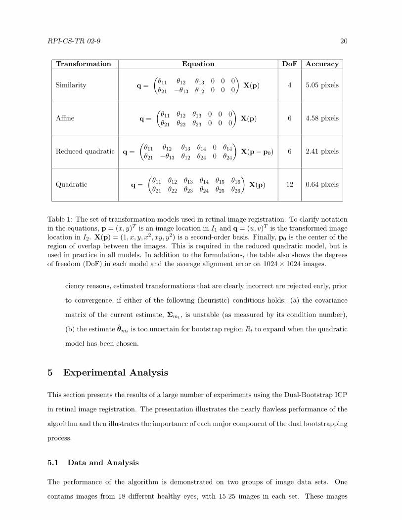
Transformation Model Set: Four transformation models have been considered: similarity,

affine, “reduced quadratic” and quadratic [9, 11] as illustrated in Table 1. All but the

reduced quadratic, which is new here, have been used in retinal image registration before.

The reduced quadratic can be derived as an approximation to the change induced in a

weak-perspective camera when a sphere rotates about its center. As seen in the table, it

has the same number of degrees of freedom as the affine model, but is much more accurate.

The affine model is in fact problematic. Its extra degrees of freedom as compared to the

similarity model allow shearing, which is unrealistic for retinal imaging. In practice, we

do not use the affine model, although the model selection technique would automatically

ignore it anyway.

Termination Criteria: The termination criteria are straightforward. For a single initial esti-

mate, the Dual-Bootstrap ICP algorithm stops bootstrap region growth when the region,

Rt, encompasses the apparent area of overlap between the two images. From then on only

the model selection and robust ICP process are applied until they converge as well. If the

median matching error of the resulting transformation is sufficiently low (threshold of 1.5

pixels, as determined empirically [11]) and the quadratic transformation parameters are

sufficiently stable, this transformation is accepted as correct. In addition, purely for effi-

RPI-CS-TR 02-9 20

Transformation Equation DoF Accuracy

Similarity q =(θ11 θ12 θ13 0 0 0θ21 −θ13 θ12 0 0 0

)X(p) 4 5.05 pixels

Affine q =(θ11 θ12 θ13 0 0 0θ21 θ22 θ23 0 0 0

)X(p) 6 4.58 pixels

Reduced quadratic q =(θ11 θ12 θ13 θ14 0 θ14

θ21 −θ13 θ12 θ24 0 θ24

)X(p− p0) 6 2.41 pixels

Quadratic q =(θ11 θ12 θ13 θ14 θ15 θ16

θ21 θ22 θ23 θ24 θ25 θ26

)X(p) 12 0.64 pixels

Table 1: The set of transformation models used in retinal image registration. To clarify notationin the equations, p = (x, y)T is an image location in I1 and q = (u, v)T is the transformed imagelocation in I2. X(p) = (1, x, y, x2, xy, y2) is a second-order basis. Finally, p0 is the center of theregion of overlap between the images. This is required in the reduced quadratic model, but isused in practice in all models. In addition to the formulations, the table also shows the degreesof freedom (DoF) in each model and the average alignment error on 1024× 1024 images.

ciency reasons, estimated transformations that are clearly incorrect are rejected early, prior

to convergence, if either of the following (heuristic) conditions holds: (a) the covariance

matrix of the current estimate, Σmt , is unstable (as measured by its condition number),

(b) the estimate θ̂mt is too uncertain for bootstrap region Rt to expand when the quadratic

model has been chosen.

5 Experimental Analysis

This section presents the results of a large number of experiments using the Dual-Bootstrap ICP

in retinal image registration. The presentation illustrates the nearly flawless performance of the

algorithm and then illustrates the importance of each major component of the dual bootstrapping

process.

5.1 Data and Analysis

The performance of the algorithm is demonstrated on two groups of image data sets. One

contains images from 18 different healthy eyes, with 15-25 images in each set. These images

RPI-CS-TR 02-9 21

show a wide range of views of each retinal fundus, and some pairs of images of the same eye

have no overlap whatsoever. The second data set contains images from 40 different eyes with

various pathologies, yielding 300 image pairs. Some of these pairs were taken at the same time,

while others were taken with time differences of months or even years. Results are presented

for the two data sets separately because the second, “pathology” set is more challenging, but

much smaller. Figure 3 illustrates the Dual-Bootstrap ICP algorithm on images of an unhealthy

retina taken at the same sitting. Figure 10 illustrates the algorithm on a pair of images taken

two months apart. Figure 11 illustrates the algorithm on a pair of images of a healthy retina.

All images in our dataset are 1024× 1024 pixels.

Measuring performance requires a means of validation, preferably ground truth. Manually

generated ground truth is extremely difficult for such a large data set, and our experience is

that this is less accurate than automatic registration anyway. Fortunately, we have a multipart

alternative strategy. First, for the set of images from any given eye, we can jointly align all

images, including pairs that have little or no overlap, using a joint, multi-image mosaicing algo-

rithm [10]. This uses constraints generated from pairwise registration, and produces quadratic

transformations (see Table 1) between all pairs of images, even ones that failed pairwise regis-

tration. (Viewing the set of images as nodes in an undirected graph and the successful pairwise

registrations as edges in the graph, the only requirement is that the graph be connected.) We

then manually validate the resulting transformations by viewing the alignment of the images. It

is important to note that no image in our data set was left out by this technique! We therefore

have “correct” transformations for all possible image pairs in our data set. The alignment error

averages less than 1 pixel.

Having these validated transformations is the basis for the crucial next step: developing

approximate upper bounds on the performance of point-based registration. Taking the set of

vascular landmarks and centerline points for each image as given and fixed, we ask the question,

“what is the best possible performance of an ICP-like registration algorithm?” Referring back

to the objective function in Equation 1, for any pair of images we can start from the “correct”

transformation and therefore find an excellent approximation to the correct set of matches (again,

with the point sets fixed). From there we can determine the covariance of the transformation

estimate. If the condition number of this matrix indicates that the transformation is sufficiently

stable, we say that a point-based registration between these image pairs is possible. Denoting

RPI-CS-TR 02-9 22

(a) (b)

(c) (d)

(e) (f)

Figure 10: Illustrating the Dual Bootstrap ICP retinal image registration algorithm on a pair ofimages from an unhealthy eye taken taken 2 months apart. The images are shown in panels (a)and (b). The vascular centerline points and landmarks are shown in (c) and (d). Panel (e) showsthe alignment of the two images based on a locally-correct initial transform. Panel (f) shows thefinal global alignment estimated by the Dual-Bootstrap ICP algorithm starting from this initialestimate.

RPI-CS-TR 02-9 23

these pairs as Mh and Mp for the healthy and pathology sets respectively, we can measure

the success rate of our algorithm as a percentage of the sizes of these two sets. This is our

first performance bound. Our second, and tighter bound, restricts Mh and Mp by eliminating

image pairs that have no common landmarks. We can discover this by using the “correct”

transformations to find corresponding landmarks. We refer to the reduced sets as M1h and

M1p. Success rates on these sets separates performance of initialization from performance of the

iterative minimization of the Dual-Bootstrap ICP algorithm and gives an idea of how well it does

given a reasonable starting point. The cardinalities of these sets are |Mh| = 5, 753, |Mp| = 369,

|M1h| = 5, 611, and |M1

p| = 361.

5.2 Overall Performance

The first and most important measure of overall performance is the success rate — the percentage

of image pairs for which a correct (within 1.5 pixels of error) transformation estimate is obtained.

This is summarized in the following table for the healthy-eye and pathology-eye datasets:

all pairs one landmark pairshealthy — Mh (%) 97.0 99.5pathology — Mp (%) 97.8 100

Table 2: Overall success rate of the Dual-Bootstrap ICP retinal image registration algorithm onhealthy-eye and pathological-eye images. The first column, labeled “all pairs”, is for all “correct”image pairs — the sets Mh and Mp. The second column, labeled “one landmark”, is for all“correct” image pairs having at least one common landmark — the sets M1

h and M1p.

These numbers are extremely high, and show virtually flawless performance of the overall

registration algorithm, including initialization, and the Dual-Bootstrap ICP algorithm in partic-

ular. (By comparison, our previous retinal image registration algorithm [11], which was based

on matching landmarks and their surroundings, was 67.1% for the healthy-eye set, Mh.) The

few failures are due to having few common landmarks or a combination of sparse centerline trace

points and low overlap. This is illustrated using a bar chart in Figure 12. To reinforce this,

for image pairs that overlap in at least 35% of the pixels and have at least one correspondence,

there were no failures. This involved over 4000 image pairs. An example pair for which the algo-

rithm failed in shown in Figure 13. These images have 32% overlap and one common landmark.

This performance means that the overall algorithm is ready for large-scale clinical testing and

RPI-CS-TR 02-9 24

(a) (b)

(c) (d)

(e) (f)

Figure 11: Illustrating the Dual Bootstrap ICP retinal image registration algorithm on a healthy-eye image pair that has 50% overlap. The images are shown in panels (a) and (b). The vascularcenterline points and landmarks are shown in (c) and (d). Panel (e) shows the alignment of thetwo images based on a locally-correct initial transform. Panel (f) shows the final global alignmentestimated by the Dual-Bootstrap ICP algorithm starting from this initial estimate.

RPI-CS-TR 02-9 25

application to change detection and visualization.

As an aside, the apparently counter-intuitive result that the pathology data set has higher

success rate is explained by the pathology image pairs having higher overlap, on average. The

healthy-eye images were deliberately taken to obtain complete views of the fundus, whereas the

pathology-eye images were taken to capture the diseased region(s).

0 0.1 0.2 0.3 0.4 0.5 0.6 0.7 0.8 0.9 10

0.1

0.2

0.3

0.4

0.5

0.6

0.7

0.8

0.9

1

fraction of overlap

succ

ess

rate

Dual_Bootstrap ICPStable

Figure 12: Plotting the percentage of successful retinal image registrations as a function ofoverlap between images. The plots include all image pairs, not just those for which a stabletransformation is available. The percentage for the Dual-Bootstrap ICP based algorithm andthe percentage of stable transformation are both shown for each interval. When the two heightsare equal, 100% success was obtained by Dual-Bootstrap ICP. Plotting the results this way showsthe overall difficulty in obtaining enough information to register at extremely low overlaps. Evenhere, however, the success rate of the algorithm nearly matches the best possible for a fixed setof points.

As a final indication of the overall algorithm, here is a summary of some additional experi-

mental details:

• Using matching of single landmarks between images resulted in a 96.7% success rate,

whereas matching pairs of landmarks from each image resulted in a 90.4% success rate.

Since the overall performance was 97.0%, the combination of both ded improve perfor-

mance, although single landmark matching alone was nearly as effective.

• The growth rate parameter, β, which is the only tuning parameter, had little effect on

the overall success rate of the algorithm. We tested values of β ranging from 0.25, which

RPI-CS-TR 02-9 26

(a) (b)

(c) (d)

Figure 13: Two images having 32% overlap and one common landmark where the Dual-BootstrapICP retinal image registration algorithm failed. The images are shown in (a) and (b) and thelandmarks and traces are shown in (c) and (d) with the common landmark circled. There aresignificant missing traces in (d). This problem has been fixed in the latest version of the tracingalgorithm.

corresponds to growing the area by at most a factor of 1.56 per iteration, to 1.0, which

corresponds to maximum area growth factor of 4 per iteration, without changing the success

rate of the algorithm. Values of β beyond 1.0 caused a very gradual reduction in the

effectiveness, with β = 8 still having a 96.6% success rate on Mh.

• The value of β =√

2 − 1, which corresponds to at most doubling the area in each itera-

tion, resulted in a median of 10 bootstrapping iterations. Larger values of β caused fewer

iterations. For example, β = 1.0 caused a median of 6 iterations.

• Over the entire dataset, including both healthy and pathology eye images, the median

RPI-CS-TR 02-9 27

number of matches tried before the algorithm succeeded was 1 and the average was 5.5.

The large difference between the median and the average is caused by a small number of

image pairs that required an extremely large number of initial estimates before success.

The worst was 746.

• The execution time required by the algorithm varied considerably with the number of initial

estimates required before success. On a 933MHz Pentium III computer running FreeBSD,

the median time was 5 seconds. Much of the time was taken in building the matching

database for pairs. Eliminating the use of pairs reduced the median time to 3.5 seconds.

5.3 Evaluation of Dual-Bootstrapping

Given the nearly flawless performance of our retinal image registration algorithm, the crucial

issue is how much of it is due to the Dual-Bootstrap ICP formulation. We can address this

by removing each of the three major components from the Dual-Bootstrap algorithm in turn:

region growth, model selection, and robust estimation. The results are summarized in Table 3

and discussed as follows.

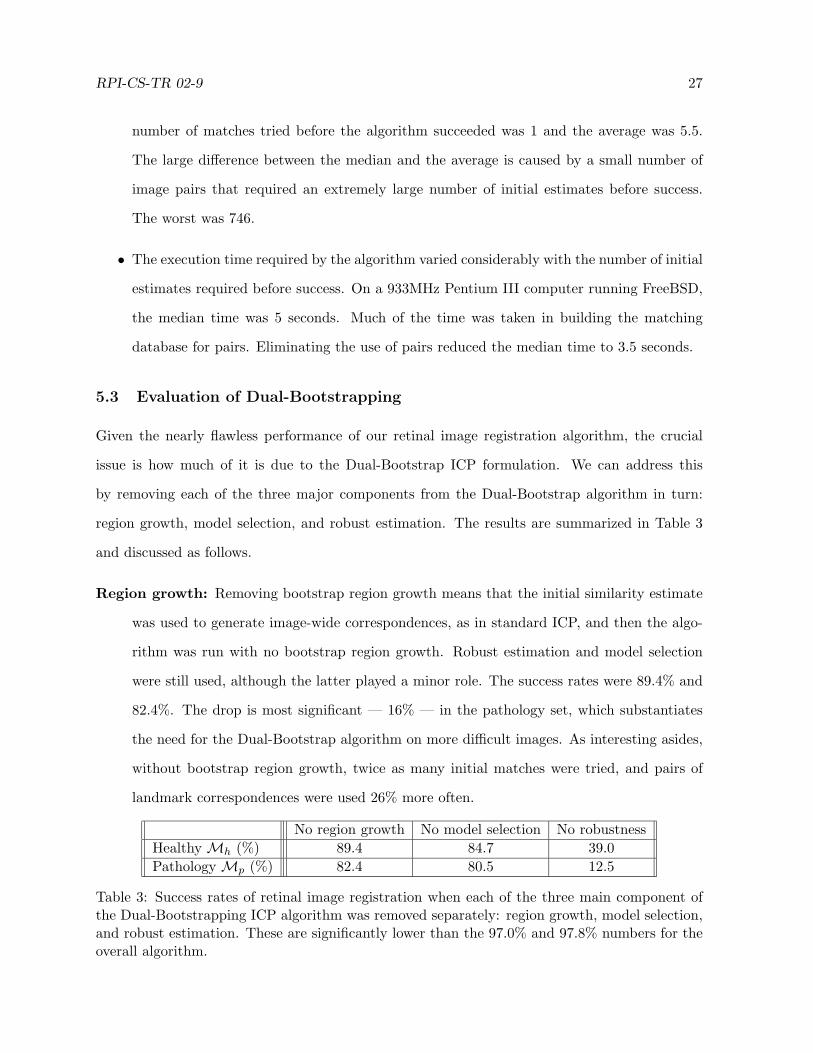
Region growth: Removing bootstrap region growth means that the initial similarity estimate

was used to generate image-wide correspondences, as in standard ICP, and then the algo-

rithm was run with no bootstrap region growth. Robust estimation and model selection

were still used, although the latter played a minor role. The success rates were 89.4% and

82.4%. The drop is most significant — 16% — in the pathology set, which substantiates

the need for the Dual-Bootstrap algorithm on more difficult images. As interesting asides,

without bootstrap region growth, twice as many initial matches were tried, and pairs of

landmark correspondences were used 26% more often.

No region growth No model selection No robustnessHealthy Mh (%) 89.4 84.7 39.0Pathology Mp (%) 82.4 80.5 12.5

Table 3: Success rates of retinal image registration when each of the three main component ofthe Dual-Bootstrapping ICP algorithm was removed separately: region growth, model selection,and robust estimation. These are significantly lower than the 97.0% and 97.8% numbers for theoverall algorithm.

RPI-CS-TR 02-9 28

Model selection: When bootstrap model selections was eliminated, a single model was used

for the entire process of bootstrap region growth and robust ICP refinement. The natural

model to use is the quadratic. The first set of quadratic parameters was estimated from the

correspondences in the initial bootstrap region. Using the quadratic model only led to a low

success rate, as shown in Table 3. On the other hand, when we initialized an intermediate

model — the reduced quadratic — from the initial bootstrap region, allow the algorithm

to run to convergence, and then switch to the quadratic transformation, performance was

much better: 94.1% on the healthy-eye set and 94.6% on the pathology-eye set. The reason

for this improvement is that the reduced quadratic is relatively accurate without requiring

too many constraints. Still, however, model selection is important for the most difficult

image pairs. Using the similarity transformation for bootstrap region growth is worse than

reduced quadratic — 91.7% and 93.0% — but not as bad as the quadratic.

Robust estimation: At first thought, the dual-bootstrapping process might seem to eliminate

the need for robust estimation, because the growth process ensures reliable correspon-

dences. This is not true, of course. By replacing the Beaton-Tukey ρ function with a

least-squares ρ function, the performance became dramatically worse (Table 3). This is

because mismatches are still clearly possible. If matching was limited to distances based on

a combination of modeling and transfer error (as will be discussed in detail in Section 6),

then robust estimation would not be as important. But, clearly this would be its own

form of robust estimation and use what amounts to a truncated quadratic. Finally, further

experiments showed that the use of MUSE scale estimator over a more common estimator

such as median absolute deviation [57] improved the effectiveness of the overall algorithm

(93.3% and 88.3%).

Clearly, these experiments show that all components of the Dual-Bootstrap algorithm are im-

portant, with importance increasing substantially for the more difficult pathology eye data set.

6 Discussion

The Dual-Bootstrap ICP algorithm has been described in general terms and then implemented

and tested in a complete technique for retinal image registration. The results far outperform any

RPI-CS-TR 02-9 29

current algorithm for this specific application. We have claimed that the algorithm is broadly

useful, however. To establish this, it is important to compare the Dual-Bootstrap ICP algorithm

(a) to other techniques that have been used to improve ICP and (b) more generally to other point-

based registration algorithms. It is also important to establish mathematically the conditions

under which it should be used rather than standard (but robust) ICP. Finally, we must consider

circumstances under which the algorithm might fail.

6.1 Comparison to Related Techniques

We compare the Dual-Bootstrap ICP algorithm to five classes of techniques that have been used

to improve ICP:

• Several published papers have used genetic algorithms and simulated annealing for a broad

search of the landscape of possible parameter estimates [5, 13, 15, 45]. Closest point

correspondences are used to evaluate each parameter estimate, with eventual application

of ICP for final refinement. The Dual-Bootstrap ICP makes such coarse search techniques

unnecessary if locally-accurate bootstrap region estimates can be obtained. Indeed, for the

retinal image registration problem our algorithm appears to be far better than currently

published techniques using genetic algorithms and simulated annealing [47, 56], based on

the results reported in the papers.

• When a significant number of distinctive features can be obtained, geometric hashing is an

efficient, reliable alignment method, especially for similarity transformations [30]. Clearly,

this assumes much more about the quality of the data than the Dual-Bootstrap ICP algo-

rithm.

• By enriching the feature set, matching can be improved, both prior to ICP and during ICP

[44, 65, 74]. Both lead to a broader domain of convergence. This approach is complementary

to the Dual Bootstrap ICP algorithm, which is designed to maximize the effectiveness of

registration for a given, fixed registration point (feature) set. Enriched features and Dual-

Bootstrap ICP can be used in combination.

• Multiresolution techniques have been used for many years in registration [24, 62, 63] and

a variety of other applications [2]. Multiresolution works from coarse descriptions of the

RPI-CS-TR 02-9 30

entire image / data set and (perhaps) simpler models, using the results at coarse resolu-

tions as starting points for finer resolution refinement. By contrast the Dual-Bootstrap

ICP algorithm, together with appropriate initialization techniques, takes a local-to-global

approach, focusing on small regions of the data first and then expanding to cover the en-

tire data set. The Dual-Bootstrap ICP algorithm could be combined with multiresolution

methods by applying it at the coarsest resolution.

• Robust techniques based on minimal subset random-sampling have been used for difficult

registration and transformation estimation problems [33, 76, 77, 79], including applications

of ICP [13, 46]. The difference that the Dual-Bootstrap ICP algorithm offers is important.

Minimal subset random sampling [26, 58] requires a sufficient set of correspondences to

generate a full model. When using the Dual-Bootstrap ICP algorithm, a much weaker

initial model may be used, with fewer initial correspondences. This implies that the Dual-

Bootstrap ICP algorithm can succeed where minimal subset random sampling fails.

• The final comparison is to the robust point matching (RPM) algorithm [17]. This uses a soft

assignment of point correspondences, smoothing-spline transformations, and deterministic

annealing to align point sets. Thus, it globally considers all matches and gradually refines

the matches and the spline transformation parameters simultaneously. This contrasts with

the Dual-Bootstrap ICP local (small region) to global (large region) refinement with gradual

incorporation of more matches. Intuitively, therefore, the Dual-Bootstrap ICP approach

seems more applicable to situations where information in small data regions provides a

“toe-hold” on the alignment. Still, because the two algorithms have been used in very

different contexts, further evaluation, perhaps on an experimental test-bed, is needed.

6.2 Utility

Since the ICP algorithm and its variants have been used successfully in a variety of applications,

it is important to address the issue of when the more sophisticated Dual-Bootstrap ICP should be

used instead. The answer is that it depends on the quality of the data, the structural complexity

of the data, and the accuracy of the initial model and parameter estimates. The following

sketches an analysis method to indicate when the Dual-Bootstrap ICP should be considered.

Suppose θ̂0 is an initial parameter estimate obtained using initial model M0. Suppose Σ0 is

RPI-CS-TR 02-9 31

the associated parameter estimate covariance matrix. In applying the standard ICP algorithm,

all points p ∈ P throughout the entire image (see Equation 1) are mapped from I1 to I2 based

on this initial estimate. Our goal is to calculate the uncertainty of this mapping, based on both

the modeling error and the transfer error for this initial estimate, and relate this to the structure

of the data.

In order to determine the modeling error, let θ0 be the optimal estimate based on the initial

model M0, and let θf be the optimal estimate based on the true/final model Mf . (Optimality

here is taken in an asymptotic sense of an estimate from a large number of correct, noise-free

correspondences.) Then, the modeling error at point p is

em(p) = d(M0(θ0; p),Mf (θf ; p)).

This is the distance between optimally mapping a point based on the initial and final models.

Clearly, if the initial and final models are the same, ep = 0.

In order to obtain the transfer error, let p′ = M0(θ0; p) be the transformation of p ∈ P.

Referring back to Equation 3, the transfer error covariance matrix of p′ is

Σp′ = J(p) Σ0 J(p)T .

Let σ2p be the maximum eigenvalue of Σp′ . This gives the maximum transfer error variance

in any direction at p′. Assuming some reasonable multiplier on the standard deviation, such

as µ = 2.5, the upper bound on the transfer error of point p due to uncertainty in the initial

estimate is

et(p) = µσp.

Finally, the combined modeling and transfer error at point p can then be defined as,

e(p) = ep + µσp

and the maximum error can be defined as

e0 = maxp∈P

e(p).

RPI-CS-TR 02-9 32

This may be interpreted by comparing e0 against the structure of the data. If e0 is larger

than or even comparable to the distance between different geometric structures in the data —

different blood vessels, different nerve fibers, different layers of the brain, different surfaces of a

complicated object — then there is substantial potential for ICP mismatches. In this case, the

Dual-Bootstrap ICP should be used in place of “standard” ICP.

Before ending this section, we offer a slightly different view on the utility of the Dual-

Bootstrap ICP algorithm. Because it works robustly from only a “toe-hold” on the alignment

between two datasets, it reduces the requirements on initialization. This can lead to a new way of

thinking about approaching a registration or alignment problem. Less cleaning and prefiltering

of the data is needed and more aggressive feature extraction and initialization techniques can be

applied. This could lead to new methods and new successes on previously difficult registration

or even recognition problems.

6.3 Potential Failures

Two conditions where the Dual-Bootstrap ICP algorithm may fail to converge following a locally

correct initialization should be mentioned:

• This first may occur when the transition between models is not captured by the match-

ing constraints generated by a low-order model. A simple, artificial example is registering

two rectangles that have a significant scaling between them by starting at a single corner

and using a Euclidean transformation (rotation and translation, no scale). Only when

the bootstrap region grows large enough to include a second corner (third side) are con-

straints available to estimate scale. At this point the implicit scale (1.0) of the Euclidean

transformation may be too far off of the true similarity transformation scale for correct

matching.

• A second condition is when each data set has two or more geometrically separated clusters

and the initial transformation is estimated only in a single cluster. As the gap between

clusters grows, the transfer error will grow with it, potentially leading to mismatches when

the bootstrap region Rt grows to include a second cluster.

While both examples are artificial, they do help to illuminate the Dual-Bootstrap method further.

The first case shows that taking the idea of weak initial estimates too far can be problematic,

RPI-CS-TR 02-9 33

especially if it ignores information, such as clean corners, available in the data. If such a cir-

cumstance were to occur in the data, then a more sophisticated method of transitioning between

models would be needed. The second case has actually appeared in rough form in our retinal

image registration experiments due to a large region of missing data. In such circumstances, the

use of accurate models becomes crucial, and this led to the discovery and introduction of the

reduced quadratic transformation.

7 Conclusions

We have introduced and applied a new generalization of the Iterative Closest Point (ICP) algo-

rithm. The Dual-Bootstrap ICP algorithm starts from an initial estimate that is only assumed to

be accurate over a small region. Using the covariance matrix of the estimated transformation pa-

rameters as its guide, it “bootstraps” both the region over which the model is applied and choice

of transformation models. It uses a robust version of standard ICP in each bootstrap iteration.

In the context of retinal image registration, when combined with an initialization technique based

on matching single landmarks or pairs of landmarks, it has shown nearly flawless performance in

matching a large set of retinal image pairs. The Dual-Bootstrap ICP algorithm should be used

in place of standard ICP when the combination of modeling and point transfer error of an initial

transformation is comparable to the distance between different curves or surfaces in the data.

Viewed another way, it substantially reduces the requirements on initial matching conditions in

a registration or alignment problem so that only a “toe hold” on the alignment is required of an

initial transformation.

The development of the algorithm raises additional challenges in registration, and these are

the focus of our ongoing work. Most importantly, in the context of retinal image registration,

the success of the algorithm, somewhat counter-intuitively, has thrown the research challenge

back at feature extraction. The algorithm so successfully exploits whatever data are available

that truly the only cause of failure is extremely poor quality image data leading to substantial

missed or spurious features. Thus, robust, low-contrast feature extraction is our ongoing focus

in retinal image registration.

RPI-CS-TR 02-9 34

8 Acknowledgements

The authors would like to thank the staff at the Center for Sight, especially Dr. Howard Tanen-

baum and Dr. Anna Majerovics, for help in understanding retinal diseases and diagnostic tech-

niques. We are thankful to Dr. Ali Can for discussions and valuable suggestions. Various portions

of this research was supported by the National Science Foundation Experimental Partnerships

grant EIA-0000417, the Center for Subsurface Sensing and Imaging Systems, under the Engi-

neering Research Centers Program of the National Science Foundation (Award Number EEC-

9986821), the National Institutes for Health grant RR14038, and by Rensselaer Polytechnic

Institute.

References

[1] R. Benjemaa and F. Schmitt. Fast global registration of 3d sampled surfaces using a multi-

z-buffer technique. Image and Vision Computing, 17(2):113–123, 1999.

[2] J. Bergen, P. Anandan, K. Hanna, and R. Hingorani. Hierarchical model-based motion

estimation. In Proceedings Second European Conference on Computer Vision, pages 237–

252, 1992.

[3] P. Besl and N. McKay. A method for registration of 3-d shapes. IEEE Transactions on

Pattern Analysis and Machine Intelligence, 14(2):239–256, 1992.

[4] T. Binford and T. Levitt. Quasi-invariants: Theory and exploitation. In Proceedings of the

DARPA Image Understanding Workshop, pages 819–829, 1993.

[5] G. Blais and M. Levine. Registering multiview range data to create 3d computer objects.

IEEE Transactions on Pattern Analysis and Machine Intelligence, 17(8):820–824, August

1995.

[6] G. Borgefors. Distance transformations in digital images. Computer Vision, Graphics, and

Image Processing, 34(3):344–371, June 1986.

[7] K. Bubna and C. V. Stewart. Model selection techniques and merging rules for range data

segmentation algorithms. Computer Vision and Image Understanding, 80:215–245, 2000.

RPI-CS-TR 02-9 35

[8] A. Can, H. Shen, J. N. Turner, H. L. Tanenbaum, and B. Roysam. Rapid automated

tracing and feature extraction from live high-resolution retinal fundus images using direct

exploratory algorithms. IEEE Trans. on Info. Tech. for Biomedicine, 3(2):125–138, 1999.

[9] A. Can, C. Stewart, and B. Roysam. Robust hierarchical algorithm for constructing a mosaic

from images of the curved human retina. In Proceedings IEEE Conference on Computer

Vision and Pattern Recognition, pages 286–292, 1999.

[10] A. Can, C. Stewart, B. Roysam, and H. Tanenbaum. A feature-based algorithm for joint, lin-

ear estimation of high-order image-to-mosaic transformations: Mosaicing the curved human

retina. IEEE Transactions on Pattern Analysis and Machine Intelligence, 24(3):412–419,

2002.

[11] A. Can, C. Stewart, B. Roysam, and H. Tanenbaum. A feature-based, robust, hierarchical

algorithm for registering pairs of images of the curved human retina. IEEE Transactions on

Pattern Analysis and Machine Intelligence, 24(3):347–364, 2002.

[12] G. Champleboux, S. Lavallee, R. Szeliski, and L. Brunie. From accurate range imaging

sensor calibration to accurate model-based 3-d object localization. In Proceedings IEEE

Conference on Computer Vision and Pattern Recognition, pages 83–89, 1992.

[13] C. Chen, Y. Hung, and J. Cheng. RANSAC-based DARCES: A new approach to fast

automatic registration of partially overlapping range images. IEEE Transactions on Pattern

Analysis and Machine Intelligence, 21(11):1229–1234, November 1999.

[14] Y. Chen and G. Medioni. Object modeling by registration of multiple range images. Image

and Vision Computing, 10(3):145–155, 1992.

[15] C. K. Chow, H. T. Tsui, T. Lee, and T. K. Lau. Medical image registration and model

construction using genetic algorithms. In Proc. of Int. Workshop on Medical Imaging and

Augmented Reality, pages 174–179, 2001.

[16] C. Chua and R. Jarvis. 3d free-form surface registration and object recognition. International

Journal of Computer Vision, 17(1):77–99, 1996.

[17] H. Chui and A. Rangarajan. A new algorithm for non-rigid point matching. In Proceedings

IEEE Conference on Computer Vision and Pattern Recognition, pages II:44–51, 2000.

RPI-CS-TR 02-9 36

[18] T. Clark, W. Freeman, and M. Goldbaum. Digital overlay of fluorescein angiograms and

fundus images for treatment of subretinal neovascularization. Retina, 12:118–26, 1992.

[19] A. Collignon, D. Vandermeulen, P. Suetens, and G. Marchal. Registration of 3d multi-

modality medical images using surfaces and point landmarks. Pattern Recognition Letters,

15(5):461–467, 1994.

[20] M. Colthurst, R. Williams, P. Hiscott, and I. Grierson. Biomaterials used in the posterior

segment of the eye. Biomaterials, 21(7):649–665, April 2000.

[21] P.-E. Danielsson. Euclidean distance mapping. Computer Graphics and Image Processing,

14:227–248, 1982.

[22] J. S. Duncan and N. Ayache. Medical image analysis: progress over two decades and

the challenges ahead. IEEE Transactions on Pattern Analysis and Machine Intelligence,

22(1):85–105, 2000.

[23] J. Feldmar and N. Ayache. Rigid, affine and locally affine registration of free-form surfaces.

International Journal of Computer Vision, 18(2):99–119, 1996.

[24] J. Feldmar, J. Declerck, G. Malandain, and N. Ayache. Extension of the ICP algorithm

to nonrigid intensity-based registration of 3d volumes. Computer Vision and Image Under-

standing, 66(2):193–206, May 1997.

[25] S. Fine. Observations following laser treatment for choroidal neovascularization. Archives

of Ophthalmology, 106:1524–1525, 1988.

[26] M. A. Fischler and R. C. Bolles. Random Sample Consensus: A paradigm for model fitting

with applications to image analysis and automated cartography. CACM, 24:381–395, 1981.

[27] K. Fritzsche, A. Can, H. Shen, C. Tsai, J. Turner, H. Tanenbuam, C. Stewart, and

B. Roysam. Automated model based segmentation, tracing and analysis of retinal vas-

culature from digital fundus images. In J. S. Suri and S. Laxminarayan, editors, State-

of-The-Art Angiography, Applications and Plaque Imaging Using MR, CT, Ultrasound and

X-rays. Academic Press, 2002.

RPI-CS-TR 02-9 37

[28] D. Geroski and H. Edelhauser. Transscleral drug delivery for posterior segment disease.

Advanced Drug Delivery Reviews, 52(1):37–48, Oct 2001.

[29] W. Grimson, T. Lozano-Perez, W. Wells, G. Ettinger, and S. White. An automatic regis-

tration method for frameless stereotaxy, image, guided surgery and enhanced reality visu-

alization. In Proceedings IEEE Conference on Computer Vision and Pattern Recognition,

pages 430–436, 1994.

[30] A. Gueziec, X. Pennec, and N. Ayache. Medical image registration using geometric hashing.

IEEE Computational Science and Engineering, 4(4):29 –41, 1997.

[31] F. R. Hampel, P. J. Rousseeuw, E. Ronchetti, and W. A. Stahel. Robust Statistics: The

Approach Based on Influence Functions. John Wiley & Sons, 1986.

[32] C. Harris and M. Stephens. A combined corner and edge detector. In Proc. 4th Alvey Vision

Conference, pages 147–151, 1988.

[33] R. Hartley and A. Zisserman. Multiple View Geometry. Cambridge University Press, 2000.

[34] T. Hellstedt and I. Immonen. Disappearance and formation rates of microaneurysms in

early diabetic retinopathy. Br. J. Ophthalmology, 6:135–139, 1999.

[35] K. Higuchi, M. Hebert, and K. Ikeuchi. Building 3-d models from unregistered range images.

Graphical Models and Image Processing, 57(4):315–333, 1995.

[36] P. W. Holland and R. E. Welsch. Robust regression using iteratively reweighted least-

squares. Commun. Statist.-Theor. Meth., A6:813–827, 1977.

[37] P. J. Huber. Robust Statistics. John Wiley & Sons, 1981.

[38] A. Johnson and M. Hebert. Surface matching for object recognition in complex 3-dimensional

scenes. Image and Vision Computing, 16(9-10):635–651, July 1998.

[39] A. Johnson and S. Kang. Registration and integration of textured 3-d data. Image and

Vision Computing, 17(2):135–147, 1999.

[40] R. Kaiser, J. Berger, M. Maguire, A. Ho, N. Javornik, and C. N. P. T. S. Group. Laser

burn intensity and the risk for choroidal neovascularization in the cnvpt fellow eye study.

Archives of Ophthalmology, 119(6):826–832, Jun 2001.

RPI-CS-TR 02-9 38

[41] C. Klaver, J. Assink, R. van Leeuwen, R. Wolfs, J. Vingerling, T. Stijnen, A. Hofman, and

P. de Jong. Incidence and progression rates of age-related maculopathy: the rotterdam

study. Investigative Ophthalmology & Visual Science, 42(10):2237–2241, Sep 2001.

[42] E. Kohner, I. Sleightholm, S. Aldington, R. Turner, and D. Matthews. Microaneurysms in

the development of diabetic retinopathy. Diabetologia, 42:1107–1112, 1999.

[43] M. Levoy, K. Pulli, B. Curless, S. Rusinkiewicz, S. Anderson, J. Davis, J. Ginsberg, J. Shade,

and D. Fulk. The Digital Michelango Project: 3d scanning of large statues. In Proceedings

of SIGGRAPH 2000, pages 131–144, 2000.

[44] Y. Liu and M. Rodrigues. Eliminating false matches in image registration through geometric

histograms from reflected correspondence vectors. In Proc. Int. Conf. on Intelligent Robots

and Systems, volume 4, pages 1997–2002, 2001.

[45] J. Luck, C. Little, and W. Hoff. Registration of range date using a hybrid simulated annealing

and iterative cloest point algorithm. In Proceedings IEEE International Conference on

Robotics and Automation, pages 3739–3744, April 2000.

[46] T. Masuda and N. Yokoya. A robust method for registration and segmentation of multiple

range images. Computer Vision and Image Understanding, 61(3):295–307, 1995.

[47] G. K. Matsopoulos, N. A. Mouravliansky, K. K. Delibasis, and K. S. Nikita. Automatic

retinal image registration scheme using global optimization techniques. IEEE Transactions

on Information Technology in Biomedicine, 3(1):47–60, 1999.

[48] D. Matthews, E. Kohner, S. Aldington, and I. Stratton. Relationship of microaneurysms

count to progression of retinopathy over 6 years in non-insulin-dependent diabetes. Diabetes,

9:117A, 1995.

[49] C.-H. Menq, H.-T. Yau, and G.-Y. Lai. Automated precision measurement of surface profile

in CAD-directed inspection. IEEE Transactions on Robotics and Automation, 8(2):268–278,

1992.

[50] J. V. Miller. Regression-Base Surface Reconstruction: Coping with Noise, Outliers, and

Discontinuities. PhD thesis, Rensselaer Polytechnic Institute, 1997.

RPI-CS-TR 02-9 39

[51] J. V. Miller and C. V. Stewart. MUSE: Robust surface fitting using unbiased scale estimates.

In Proceedings IEEE Conference on Computer Vision and Pattern Recognition, pages 300–

306, 1996.

[52] R. Mittre and W. Mieler. Retina, volume 2, chapter 111. Drug Toxicity of the Posterior

Segment. Mosby, 2001. 1779–1796.

[53] J. Mundy and A. Zisserman, editors. Geometric Invariance in Computer Vision. MIT Press,

1992.

[54] V. Murino, L. Ronchetti, U. Castellani, and A. Fusiello. Reconstruction of complex envi-

ronments by robust pre-aligned ICP. In Proc. Third Int. Conf. on 3-D Digital Imaging and

Modeling, pages 187–194, 2001.

[55] V.-D. Nguyen, V. Nzomigni, and C. Stewart. Fast and robust registration of 3d surfaces

using low curvature patches. In Proc. 2nd Int. Conf. on 3D Digital Imaging and Modeling,

pages 201–208, 1999.

[56] N. Ritter, R. Owens, J. Cooper, R. Eikelboom, and P. van Saarloos. Registration of stereo

and temporal images of the retina. IEEE Transactions on Medical Imaging, 18(5):404–418,

1999.

[57] P. J. Rousseeuw. Least median of squares regression. Journal of the American Statistical

Association, 79:871–880, 1984.

[58] P. J. Rousseeuw and C. Croux. Alternatives to the median absolute deviation. Journal of

the American Statistical Association, 88:1273–1283, 1993.

[59] P. J. Rousseeuw and A. M. Leroy. Robust Regression and Outlier Detection. John Wiley &

Sons, 1987.

[60] S. Rusinkiewicz and M. Levoy. Efficient variants of the ICP algorithm. In Proc. Third Int.

Conf. on 3-D Digital Imaging and Modeling, pages 224 –231, 2001.

[61] S. Russell and G. Hageman. Optic disc, foveal, and extrafoveal damage due to surgical

separation of the vitreous. Archives of Ophthalmology, 119(11):1653–1658, Nov 2001.

RPI-CS-TR 02-9 40

[62] H. Sawhney, S. Hsu, and R. Kumar. Robust video mosaicing through topology inference

and local to global alignment. In Proceedings 5th European Conference on Computer Vision,

volume II, pages 103–119, 1998.

[63] H. Sawhney and R. Kumar. True multi-image alignment and its application to mosaicing and

lens distortion correction. IEEE Transactions on Pattern Analysis and Machine Intelligence,

21(3):235–243, 1999.

[64] C. Schmid, R. Mohr, and C. Bauckhage. Comparing and evaluating interest points. In

Proceedings IEEE International Conference on Computer Vision, pages 230–235, 1998.

[65] G. Sharp, S. Lee, and D. Wehe. ICP registration using invariant features. IEEE Transactions

on Pattern Analysis and Machine Intelligence, 24(1):90–102, 2002.

[66] H. Shen, B. Roysam, C. Stewart, J. Turner, and H. Tanenbaum. Optimal scheduling of

tracing computations for real-time vascular landmark extraction from retinal fundus images.

IEEE Transactions on Information Technology in Biomedicine, 5(1):77–91, Mar 2001.

[67] H. Shen, C. Stewart, B. Roysam, G. Lin, and H. Tanenbaum. Frame-rate spatial referencing

based on invariant indexing and alignment with application to laser retinal surgery. In

Proceedings IEEE Conference on Computer Vision and Pattern Recognition, volume 1, pages

79–86, 2001.

[68] J. Shi and C. Tomasi. Good features to track. In Proceedings IEEE Conference on Computer

Vision and Pattern Recognition, pages 593–600, 1994.

[69] G. Soubrane, C. Coscas, G. amd Francais, and F. Koenig. Occult subretinal new vessels in

age-related macular degeneration. Ophthalmology, 97:649–657, 1990.

[70] C. V. Stewart. Robust parameter estimation in computer vision. SIAM Reviews, 41(3),

September 1999.

[71] A. Stoddart, S. Lemke, A. Hilton, and T. Renn. Estimating pose uncertainty for surface

registration. Image and Vision Computing, 16(2):111–120, 1998.

[72] R. Szeliski and S. Lavallee. Matching 3-d anatomical surfaces with non-rigid deformations

using octree-splines. International Journal of Computer Vision, 18(2):171–186, 1996.

RPI-CS-TR 02-9 41

[73] The Macular Photocoagulation Study Group. The use of fundus photographs and fluorescein

angiograms in the identification and treatment of choroidal neovascularization in the macular

photocoagulation study. Ophthalmology, 96:1526–1534, 1989.

[74] J. Thirion. New feature points based on geometric invariants for 3d image registration.

International Journal of Computer Vision, 18(2):121–137, 1996.

[75] P. Torr. An assessment of information criteria for motion model selection. In Proceedings

IEEE Conference on Computer Vision and Pattern Recognition, pages 47–52, 1997.

[76] P. Torr and D. Murray. The development and comparison of robust methods for estimating

the fundamental matrix. International Journal of Computer Vision, 24(3):271–300, 1997.

[77] P. Torr and A. Zisserman. MLESAC: A new robust estimator with application to estimating

image geometry. Computer Vision and Image Understanding, 78(1):138–156, April 2000.

[78] Z. Zhang. Iterative point matching for registration of free-form curves and surfaces. Inter-

national Journal of Computer Vision, 13(2):119–152, 1994.

[79] Z. Zhang. Determining the epipolar geometry and its uncertainty: A review. International

Journal of Computer Vision, 27(2):161–195, 1998.