submitted to ieee transactions on image processing 1 …

SUBMITTED TO IEEE TRANSACTIONS ON IMAGE PROCESSING 1

Image Co-skeletonization via Co-segmentationKoteswar Rao Jerripothula, Member, IEEE, Jianfei Cai, Senior Member, IEEE, Jiangbo Lu, Senior Member, IEEE,

and Junsong Yuan, Senior Member, IEEE

Abstract—Recent advances in the joint processing of imageshave certainly shown its advantages over individual process-ing. Different from the existing works geared towards co-segmentation or co-localization, in this paper, we explore anew joint processing topic: image co-skeletonization, which isdefined as joint skeleton extraction of objects in an imagecollection. Object skeletonization in a single natural image is achallenging problem because there is hardly any prior knowledgeabout the object. Therefore, we resort to the idea of object co-skeletonization, hoping that the commonness prior that existsacross the images may help, just as it does for other jointprocessing problems such as co-segmentation. We observe thatthe skeleton can provide good scribbles for segmentation, andskeletonization, in turn, needs good segmentation. Therefore,we propose a coupled framework for co-skeletonization and co-segmentation tasks so that they are well informed by each other,and benefit each other synergistically. Since it is a new problem,we also construct a benchmark dataset by annotating nearly1.8k images spread across 38 categories. Extensive experimentsdemonstrate that the proposed method achieves promising resultsin all the three possible scenarios of joint-processing: weakly-supervised, supervised, and unsupervised.

Index Terms—skeletonization, segmentation, joint processing.

I. INTRODUCTION

Our main objective in this paper is to exploit joint pro-cessing [2], [3], [4], [5], [6], [7], [8], [9], [10], [11], [12]to extract skeletons of the objects in natural images. We callit object co-skeletonization. By objects, we mean somethingwhich interests the viewer more compared to the backgroundregions such as sky, roads, mountains, and sea in its presence.Automatic skeletonization of such objects has many applica-tions such as image search, image synthesis, and training datageneration for object detectors [13]. However, it is difficult tosolve this problem as a standalone task, for it requires somesupport or other. In literature, existing methods either need pre-segmentation [14], [15] of the object in the image or ground-truth skeletons for the training images to learn [16], [17] toperform skeletonization on test images. Even the recent deeplearning [18], [19], [20] based method [21] (extended in [22])requires not only the skeleton location information for trainingbut also the skeleton scale information. Such scale informationessentially accounts for shape information, since it is thedistance between a skeleton point and the nearest boundarypoint of the object. Providing such additional scale annotationhas shown significant improvement in performance for [21]

A preliminary version of this work appears in CVPR’17 [1]. K. R. Jer-ripothula is with IIIT Delhi, India, J. Cai is with Monash University, Australia,J. Lu is with Shenzhen Cloudream Technology Co., Ltd. and J. Yuan is withUniversity at Buffalo, United States of America. E-mail: [email protected],[email protected], [email protected] and [email protected]. [email protected] for further questions about this work.

Source images

Skeletons Segmentations Joint Optimization

Co-segmentation Co-skeletonization

Scribbles

Shapes

Fig. 1. Image co-skeletonization via co-segmentation. Skeletons are in yellow.

over [23] that can make use of only skeleton annotations whiletaking the deep learning [24], [25], [26] approach.

In contrast, in this paper, we propose a problem calledco-skeletonization, which doesn’t need to depend upon anykind of annotations exclusively. Instead, we rely on the jointprocessing, where the central idea is to exploit the com-monness of the images. Also, inspired by [21], we leveragealready existing another joint processing idea named objectco-segmentation [2], [27], [28], [29] to provide the additionalrequired shape information to our co-skeletonization problem.Interestingly, it turns out that co-skeletonization can also helpco-segmentation in return by providing scribble informationrequired for segmentation. In this way, both co-skeletonizationand co-segmentation benefit each other synergistically. Wecouple these two tasks to achieve what we call ”Image Co-skeletonization via Co-segmentation,” as shown in Fig. 1. Un-like the existing methods like [21], [23], which function onlyin the supervised scenario, by exploiting commonness, theproposed method manages to function in all the three possiblescenarios: weakly-supervised, supervised, and unsupervised.

There are several challenges involved in performing co-skeletonization and coupling it with co-segmentation. First,existing skeletonization algorithms [15], [30], [14], [31] canyield a good skeleton provided a good and smooth shapeis provided, for they are quite sensitive to the given shape,as shown for the image in Fig. 2(a) which has unsmoothsegmentation. The skeleton produced by [15] in Fig. 2(a)has too many unnecessary branches, while a more desirableskeleton to represent the cheetah would be the one obtainedby our modified method in Fig. 2(c). Thus, the quality ofthe provided shape becomes crucial, which is challenging

arX

iv:2

004.

0557

5v1

[cs

.CV

] 1

2 A

pr 2

020


(a) (b) (c)

(d) (e)

Fig. 2. Example challenges of co-skeletonization. The quality of segmentationaffects the quality of skeletonization. (b) The result of [15] for (a). (c) Ourresult. Skeletons lie on homogeneous regions, such as in (d) and (e), whichare difficult to be detected and described.

for the conventional co-segmentation methods because theircomplicated way of co-labeling many images may not providegood and smooth shapes. Second, the joint processing ofskeletons across multiple images is quite tricky. Because mostof the skeleton points generally lie in homogeneous regions, asshown in Fig. 2(d) and (e), it is not easy to detect and describethem for matching. Third, how to couple the two tasks so thatthey can synergistically assist each other is another challenge.

Our key observation is that we can exploit the inherent inter-dependencies of the two tasks to achieve better results jointly.For example, in Fig. 3, although the initial segmentation ispoor, most of the skeleton pixels remain on the horse body.These skeleton pixels gradually improve the segmentationby providing good scribble information for segmentation inthe subsequent iterations of joint processing. In turn, skele-tonization also becomes better as the segmentation improves.Our other observation is that we can exploit the structure-preserving property of dense correspondence techniques toovercome the skeleton matching problem. Thanks to thesmoothness constraint in its optimization framework, densecorrespondence has this useful structure-preserving property.

To the best of our knowledge, there is only one datasetwhere co-skeletonization could be performed in a weakly-supervised manner (with similar images collected at oneplace), i.e., WH-SYMMAX dataset [17], and it only containshorse images. To extensively evaluate co-skeletonization onseveral categories, we constructed a benchmark dataset namedCO-SKEL dataset in our preliminary work [1]. It consisted ofimages ranging from animals, birds, flowers to humans witha total of 26 categories. However, the size of the dataset wassmall (about 350 images only). In this paper, we present alarger and more challenging dataset containing around 1.8kimages, which are categorized into 38 categories. We call thislarger dataset as the CO-SKELARGE dataset. Efficient objectskeletonization in such large datasets has been made possiblein this paper through our speeded-up extension proposed inthis paper. In the speeded-up extension, priors of key imagesare computed first, and then they are propagated to otherimages. Such an approach speeds up the process significantly.

Fig. 3. Inherent interdependencies of co-skeletonization and co-segmentationcan be exploited to achieve better results through a coupled iterative optimiza-tion process.

Moreover, since our method doesn’t depend on annotationsexclusively, we perform extensive experiments on variousdatasets using all the three approaches: weakly-supervised(only category-label annotations), supervised (skeleton andsegmentation annotations) and unsupervised (no annotations).The proposed method achieves promising results in all threescenarios.

We would like to point out that compared with our con-ference version [1], this journal submission includes the fol-lowing significant extensions. 1) We construct a larger andmore challenging dataset named CO-SKELARGE dataset.2) We employ key prior propagation idea to speed up theprocess while handling large datasets. 3) We now provide moredetailed experimental results covering all the three possiblejoint processing scenarios: weakly-supervised, supervised, andunsupervised.

II. RELATED WORK

A. Skeletonization

The research on skeletonization can be divided into threecategories. First, there are some algorithms, such as [30],[14], [31], which can perform skeletonization if the segmentedshape of the object is given. Generally, these algorithms aresensitive to distortions of the given shape. However, thisproblem can be tackled through methods such as pruning[15]. Second, there are also some traditional image processingmethods [32], [33], [34], which can generate skeletons byexploiting gradient intensity maps. However, they generateskeletons even for stuff such as sky, sea, and mountains. Insuch a case, we usually need some object mask to suppressthem. Third, there are also supervised learning based methods,which require ground-truth skeletons for some images to traina model. This class of methods includes both the traditionalmachine learning based methods [16], [17] and the recent deeplearning based methods [23], [21]. The performance of thetraditional machine learning based methods, however, is notso satisfactory due to the limited feature learning capabilityin homogeneous regions. On the contrary, the recent deeplearning based methods have made remarkable progress in theskeletonization as reported in [21], [22].Somewhat similar to


the skeletonization, there are also results reported on key-pointdetection in [26], which is an extension of [35]. However,it is all at the cost of requiring a complex training processon a substantial amount of annotated data (including key-points). Note that such methods are functional only in thesupervised scenario. In contrast, our method depends on jointprocessing and can function in all three possible scenarios:weakly-supervised, supervised, and unsupervised. Also, suchmethods can reliably be applied only to the object categoriesthat have been included during the training process. In contrast,our joint processing based method can work on any category.If there is no annotated data available for a particular category,we can always take the weakly-supervised perspective andapply our method. And, if images are not categorized also,we can then take the unsupervised perspective.

B. Segmentation

Image segmentation is a classical problem, and there aremany types of approaches like interactive segmentation [36],[37], image co-segmentation [38], [39], [40], semantic seg-mentation [41], etc. While interactive segmentation needshuman efforts, image co-segmentation exploits inter-imagecommonness prior to help segment the individual image. Dif-ferent from foreground extraction that deals only with binarylabels, semantic image segmentation deals with multiple labelsfor giving semantic meaning to each pixel. In the past fewyears, deep learning based methods such as fully convolutionnetworks (FCN) have greatly advanced the performance ofsemantic image segmentation. Later, to decrease the annotationburden, [42] proposed a joint framework to combine scribble-based interactive segmentation with FCN based semantic seg-mentation [41] so that they can assist each other. In a similarspirit, in this work, we propose to couple two tasks named co-skeletonization and co-segmentation for mutual assistance. Co-segmentation is another type of segmentation where we jointlysegment multiple images while exploiting the commonnessprior existing across them. It was introduced by Rother etal. [2] using histogram matching for accomplishing this task.Since then, many co-segmentation methods have been pro-posed to either improve the segmentation in terms of accuracyand processing speed [43], [44], [45], [46], [47], [48] or scalefrom image pair to multiple images [49], [50], [51], [52].Inspired by co-segmentation, we have introduced a new taskcalled co-skeletonization that also exploits commonness butfor the purpose of skeletonization. And since co-segmentationcan provide the required shape in co-skeletonization, wecouple these two joint processing tasks.

III. PROPOSED METHOD

In this section, we propose our joint framework for co-skeletonization and co-segmentation. The idea is to use skele-tons generated from co-skeletonization as scribbles requiredin co-segmentation and use segmentations generated from co-segmentation as shapes required in co-skeletonization. In thismanner, the two tasks become interdependent of each other.Meanwhile, commonness across the images is exploited to

generate co-skeleton and co-segment priors using structure-preserving dense correspondence. Thus, empowered by thesepriors and interdependence between the two tasks, we jointlyoptimize our co-skeletonization and co-segmentation problemswhile taking into consideration their respective smoothnessconstraints.

A. Overview of Our Approach

Given a set of m images, denoted by I = {I1, I2, · · · , Im},we aim to create two output sets: K = {K1,K2, · · · ,Km}and O = {O1, O2, · · · , Om}, comprising of skeleton masksand segmentation masks, respectively, where Ki(p), Oi(p) ∈{0, 1} indicating whether a pixel p is a skeleton pixel (Ki(p) =1) and whether it is a foreground pixel (Oi(p) = 1).

Our overall objective function for an image Ii is defined as

minKi,Oi

λψpr(Ki, Oi|Ni) + ψin(Ki, Oi|Ii) + ψsm(Ki, Oi|Ii)

s.t. Ki ⊆ma(Oi)(1)

where the first term ψpr accounts for the inter-image priorsfrom a set of neighbor images denoted as Ni, the second termψin is to enforce the interdependence between the skeletonKi and the shape/segmentation Oi in image Ii, the third termψsm is the smoothness term to enforce smoothness, and λ isa parameter to control the influence of the inter-image priorterm. The constraint in (1) means the skeleton must be a subsetof the medial axis (ma) [14] of the shape. Regarding neighborimages note that they are obtained using different approachesin different scenarios. In the weakly-supervised scenario, theyare obtained using the k-means clustering approach on therespective category of the dataset. In the supervised scenario,they are collected using the kNN approach on the trainingdataset. In the unsupervised scenario, they are obtained usingthe k-means clustering approach on the entire dataset.

We resort to the typical alternative optimization strategy tosolve (1), i.e., dividing (1) into two sub-problems and solvethem iteratively. In particular, one sub-problem is as follows.Given the shape Oi, we solve co-skeletonization by

minKi

λψkpr(Ki|Ni) + ψkin(Ki|Oi) + ψksm(Ki)

s.t. Ki ⊆ma(Oi).(2)

The other sub-problem is that given the skeleton Ki, we solveco-segmentation by

minOi

λψopr(Oi|Ni) + ψoin(Oi|Ki, Ii) + ψosm(Oi|Ii). (3)

If we treat both the inter-image prior term ψkpr and theshape prior term ψkin as a combined prior, (2) turns out tobe a skeleton pruning problem and can be solved using theapproach similar to [15], where branches in the skeleton areiteratively removed as long as it reduces the overall energy.Similarly, if we combine both the inter-image prior ψopr and theskeleton prior ψoin as the data term, (3) becomes a standardMRF-based segmentation formulation, which can be solvedusing GrabCut [36]. Thus, compared with the existing works,the key differences of our formulation lie in the designed inter-image prior terms as well as the interdependence terms, whichlink the co-skeletonization and co-segmentation together.


Weakly Supervised

Supervised

Unsupervised

Saliency Initialization

Saliency Initialization

Ground-truth Initialization

Category Labeled Dataset

Training Dataset

Completely Unlabeled

Dataset

Fig. 4. Our method works in all three scenarios: weakly-supervised, supervised and unsupervised. The dataset composition and our initialization varyaccordingly. Bordered images are the selected neighbors for the considered image.

In literature, several works have taken such an alternativeoptimization approach while combining different complicatedmodalities. A representative work is [51] where masks andcorrespondences were alternatively obtained. However, onegood thing about such an approach is that the neighborhoodsof images become better progressively if we use the resultsobtained at every iteration for seeking it, as reported in thesame work. Given that, we can be convinced that skeletonscombined with improving joint processing give better fore-ground seeds for segmentation, and segmentation combinedwith improving joint processing gives good shapes for skele-tonization. This kind of iteratively solving (2) and (3) requiresinitialization first of all. For this purpose, we propose toinitialize O by Otsu thresholded saliency maps [53] and Kby the medial axis mask [14]. From experiments, we foundthat [53] gave us the best results; otherwise, our method is notdependent on a particular method. Note that, in the supervisedscenario, the training images are initialized using ground-truthskeletons as initial skeletons. We use the same ground-truthskeletons to generate initial segmentation masks as well usinggrabcut, which are denoted by gc. We can easily generatea bounding box required in the grabcut using a skeleton.Different scenarios have been made clear in Fig. 4. Alg. 1summarizes our approach, where (ψpr+ψin+ψsm)(t) denotesthe objective function value of (1) at the tth iteration andψpr = ψkpr + ψopr, ψin = ψkin + ψoin, ψsm = ψksm + ψosm.

B. Object Co-skeletonization

As shown in Alg. 1, the step of object co-skeletonization isto obtain K(t+1) by minimizing (2), given the shape O(t+1)

and the previous skeleton set Kt. Considering the constraintof K(t+1)

i ∈ ma(O(t+1)i ), we only need to search skeleton

Algorithm 1: Our approach for solving (1). Note thatma(·) and gc(·) denote medial axis and grabcut algorithm.

Data: An image set I.Result: Sets O and K containing segmentations and

skeletons of images in IInitialization: ∀Ii ∈ I,if Ii ∈ testset then

O(0)i = Otsu thresholded saliency map andK

(0)i = ma(O

(0)i )

endelse

K(0)i = skeleton annotation and O(0)

i = gc(K(0)i )

endProcess: ∀Ii ∈ I,do

1) Obtain O(t+1)i by solving (3) using [36] with O(t)

and K(t)i .

2) Obtain K(t+1)i by solving (2) using [15] with K(t)

and O(t+1)i , s.t. K(t+1)

i ∈ma(O(t+1)i ).

while (λψpr+ψin+ψsm)(t+1) ≤ (λψpr+ψin+ψsm)(t);O ← O(t) and K ← K(t)

pixels from the medial axis pixels. We build up our solutionbased on [15], but with our carefully designed individual termsfor (2) as explained below.

Prior Term (ψkpr): In the object co-skeletonization, a goodskeleton pixel is the one that is repetitive across images. Toaccount for this repetitiveness, we need to find correspondingskeleton pixels in other images. However, skeleton pixelsusually lie in homogeneous regions (see Fig. 2(d)&(e)) and


are thus challenging to match. Thus, instead of trying to matchsparse skeleton pixels, we make use of dense correspondencesusing SIFT Flow [54], which preserve the skeleton and seg-mentation structures well, as shown in Fig. 5.

Once the correspondence is established, we utilize thewarped skeleton pixels from neighboring images to developthe prior term. Particularly, we align all the neighboringimages’ tth iteration’s skeleton maps to the concerned imageIi, and generate a co-skeleton prior at the (t + 1)th iterationas

K(t+1)i =

K(t)i +

∑Ij∈Ni

Wij(K

(t)j )

|Ni|+ 1(4)

where we align other skeleton maps using a warping functionWi

j [54] and then average them with Ii’s own skeleton map.Note that neighbors Ni are obtained in the GIST feature [55]domain. For simplicity, we drop the superscriptions such as(t+ 1) in all the following derivations.

Considering that the corresponding skeleton pixels fromother images may not exactly align with the skeleton pixelsof the considered image, we define our inter-image prior termas

ψkpr(Ki|Ni) =−∑p∈Di

Ki(p) log(1 +

∑q∈N(p)

Ki(q))

∑p∈Di

Ki(p). (5)

Eq. (5) essentially measures the consistency among image Ii’sown skeleton mask and the recommended skeleton mask fromits neighbor images. Note that Di represents pixel domain ofIi and we accumulate the co-skeleton prior scores in a certainneighborhood N(p) for each pixel p to account for the roughskeleton alignment across the images.

Interdependence Term (ψkin): Our interdependence term issimilar to the traditional data term in skeleton pruning, i.e., itenforces that the skeleton should provide a good reconstructionof the given shape, which medial axis already does well. How-ever, a medial axis often contains spurious branches, while thenoisy shapes obtained from imperfect co-segmentation onlymake this worse. To avoid spurious branches, we prefer asimplified skeleton whose reconstructed shape is expected tobe smooth while still preserving the main structure of the givenshape (see Fig. 6 for example). On the other hand, we do notwant an over-simplified skeleton whose reconstructed shape islikely to miss some important parts (see the 4th column ofFig. 6). Therefore, we expect the reconstructed shape fromthe skeleton to match the given shape, but not necessary to beexactly the same as the given shape. In this spirit, we defineour interdependence term ψkin as

ψkin(Ki|Oi) = −α log|R(Ki, Oi) ∩Oi||R(Ki, Oi) ∪Oi|

(6)

where we use IoU to measure the closeness between thereconstructed shape R(Ki, Oi) and the given shape Oi, andα is the normalization factor as defined in [15]. Note thatthis term has been differently defined compared to the [15],which uses the simple difference between the two maps.

(a) (b) (c)

Fig. 5. Dense correspondences preserve the skeleton and segmentationstructures roughly. Here (a) is warped to generate (b) to be used as a priorfor (c).

Source image

Shape & medial axis

Reconstructed shape & skeleton

Missing parts

Hump?

Leg?

Fig. 6. Shape reconstruction from skeleton. Compared to the reconstructedshape from the medial axis (2nd column), the reconstructed shape (3rdcolumn) from our simplified skeleton is simpler and smoother while stillpreserving the main structure. Nevertheless, we do not want an over-simplifiedskeleton, which will result in missing important parts in the correspondingshape reconstruction (4th column).

The reconstructed shape R(Ki, Oi) is basically the union ofmaximal disks at skeleton pixels [15], i.e.,

R(Ki, Oi) =⋃

p∈Ki|Ki(p)=1

d(p,Oi) (7)

where d(p,Oi) denotes the maximal disk at skeleton pixel pfor the given Oi, and the maximal disk is the disk that exactlyfits within Oi with skeleton pixel p as the center.

Smoothness Term (ψksm): To ensure a smoother and sim-pler skeleton, we aim for a skeleton whose: (i) branchesare less in number and (ii) branches are long. Our criteriadiscourage skeletons with spurious branches while at the sametime encouraging skeletons with structure-defining branches.This is different from the criteria in [15] which only aimsfor less number of skeleton pixels. Specifically, we define thesmoothness term ψksm as

ψksm(Ki) = |b(Ki)| ×|b(Ki)|∑u=1

1

length(bu(Ki)

) (8)

where b(Ki) = {b1(Ki), · · · , b|b(Ki)|(Ki)} denotes the set ofbranches of the skeleton Ki. In this way, we punish skeletons


having either large number of branches (through |b(Ki)|) orhaving short branches

(through 1/length

(bu(Ki)

)).

C. Object Co-segmentation

The object co-segmentation problem here is as follows.Given the skeleton Ki, find the optimal Oi that minimizesthe objective function defined in Eq. (3). The individual termsin Eq. (3) are defined in the following manner.

Prior Term (ψopr): We generate an inter-image co-segmentprior, similar to that for co-skeletonization. In particular, wealign segmentation masks of neighboring images and fusethem with that of the concerned image, i.e.,

Oi =

Oi +∑

Ij∈Ni

Wij(Oj)

|Ni|+ 1(9)

where Wij is the same warping function from image j to

image i as used object co-skeletonization. Then, with the helpof Oi, we define our inter-image prior term as

ψopr(Oi|Ni) =∑p∈Di

−

(Oi(p) log

( 1

|N(p)|∑q∈N(p)

Oi(q))

+(1−Oi(p)

)log(1− 1

|N(p)|∑q∈N(p)

Oi(q)))(10)

which encourages the shape to be consistent with Oi. Hereagain we account for pixel correspondence errors by neigh-borhood N(p) averaging in the pixel domain Di.

Interdependence Term (ψoin): For the co-segmentationprocess to benefit from co-skeletonization, our basic idea is tobuild foreground and background appearance models based onthe given skeleton Ki. Notably, we use GMM for appearancemodels. The foreground GMM model is learned using Ki

(i.e., treating skeleton pixels as foreground seeds), whereasthe background GMM is learned using the background partof Ki’s reconstructed shape R(Ki, Oi). In this manner, theappearance model is developed entirely using the skeleton.Note that, in the beginning, it is not robust to build up theGMM appearance models in this manner since the initialskeleton extracted based on saliency is not reliable at all. Thus,at initialization, we develop the foreground and backgroundappearance models based on the inter-image priors Ki andOi, respectively.

Denoting θ(Ki, Ii) as the developed appearance models, wedefine the interdependence term ψoin as

ψoin(Oi|Ki, Ii) =∑p∈Di

− log

(P(Oi(p) | θ(Ki, Ii), Ii(p)

))(11)

where P(Oi(p) | θ(Ki, Ii), Ii(p)

)denotes how likely a pixel

of color I(p) will take the label Oi(p) given θ(Ki, Ii). ψoinis similar to the data term in the interactive segmentationmethod [36].

Smoothness Term (ψosm): For ensuring smooth foregroundand background segments, we simply adopt the smoothnessterm of GrabCut [36], i.e.,

ψosm(Oi|Ii) = γ∑

(p,q)∈Ei

[Oi(p) 6= Oi(q)]e(−β||Ii(p)−Ii(q)||2)

(12)where Ei denotes the set of neighboring pixel pairs in theimage Ii, and γ and β are segmentation smoothness relatedparameters as discussed in [36].

D. Key Prior Propagation

In the approach discussed so far, particularly in weakly-supervised and unsupervised scenarios, neighbors were othermembers in a cluster. Therefore, the interaction effectivelyinvolved aligning each image w.r.t. each image in a clusterfor generating the individual priors. Note that these alignmentsare computationally expensive. So, the current approach needssome modification while dealing with large datasets. To over-come this problem, we assume that the alignment is precise,which means that the same sets of corresponding pixels gettogether every time we try to collect them for different imagesin the cluster. In case this assumption holds, collecting thepixels for each image appears to be repetitive. We can speedup this process by collecting them only once and propagateback the generated priors to others. We call such priors askey priors. For this purpose, for any cluster, we choose thenearest image of the cluster-center as the key image, say Inin the nth cluster Cn, for which we first get correspondingpixels and compute the key priors. Then we propagate thesepriors to other cluster members by aligning back for formingtheir priors. Specifically, we get key co-skeleton prior at anyiteration using

K(t+1)n =

K(t)n +

∑Ij∈Cn,Ij 6=In

Wnj (K

(t)j )

|Cn|(13)

, and the key co-segment prior is obtained as

O(t+1)n =

O(t)n +

∑Ij∈Cn,Ij 6=In

Wnj (O

(t)j )

|Cn|. (14)

As far as co-skeleton and co-segment priors of other mem-bers {Ij |Ij ∈ Cn, Ij 6= In} are concerned, they are computedusing

K(t+1)j = Wj

n(K(t)n ) and O(t+1)

j = Wjn(O

(t)n ), (15)

respectively. In our original approach, in a cluster Cn, everytime we collected corresponding pixels for an image, werequired (|Cn| − 1) alignments for one image in the cluster.Thus, total number of alignments required in a cluster becomes|Cn|(|Cn| − 1). But after this modification, we need to align(Cn − 1) times only for the key image, and then we needanother (|Cn| − 1) alignments for propagation. Thus, the totalnumber of alignments now turns out to be only 2(|Cn| − 1).There is a clear speed up of |Cn|/2 from |Cn|(|Cn| − 1) to2(|Cn|−1) in the number of alignments required using our keyprior propagation approach. Also, we speed-up our approach


from having a quadratic time-complexity to one having onlya linear time complexity.

E. Implementation Details

We use the saliency extraction method [56] for initial-ization of our framework in our experiments. Note that theproposed method is not restricted to this particular saliencyextraction method; any other method can also be used forthe initialization purpose. We use the same default settingas reported in [36] for the segmentation parameters γ andβ in (12) throughout our experiments. For the parameters ofSIFT flow [54], we follow the setting in [51] to handle thepossible matching of different semantic objects. The parameterλ in both (2) and (3), which controls the influence of jointprocessing, is set to 0.1.

IV. EXPERIMENTAL RESULTS

In this section, we first discuss the different datasets andevaluation metrics used in our experiments. Then, we discussour experiments in three joint processing scenarios, namelyweakly-supervised, supervised, and unsupervised. Lastly, weprovide some discussions and limitations. We generally reportour results using the original approach unless specified, i.e.,we specify whenever we resort to speed-up through key-priorgeneration.

A. Datasets and Evaluation Metrics

Datasets: So far, there is only one publicly available dataset,i.e. WH-SYMMAX dataset [17], on which weakly supervisedco-skeletonization can be performed, but it contains only thehorse category of images. To evaluate the weak-supervised co-skeletonization task extensively, we develop a new benchmarkdataset named CO-SKELARGE dataset. Its initial versionnamed CO-SKEL was presented in our preliminary work [1].While the CO-SKEL dataset consisted of 26 categories witha total of 348 images of animals, birds, flowers, and humans,the CO-SKELARGE dataset consists of 38 categories and atotal of 1831 images. These images are collected from variouspublicly available datasets such as MSRC, CosegRep, andWeizmann Horses along with their ground-truth segmentationmasks. We apply [15] (with our improved terms) on theseground-truth masks, just like the way WH-SYMMAX datasetwas developed from the Weizmann Horses dataset [57]. Fig. 7shows some example images, and their skeletons using [15]and our improvement of [15]. Thanks to our improved terms,it can be seen that our skeletons are much smoother and betterin representing the shapes.

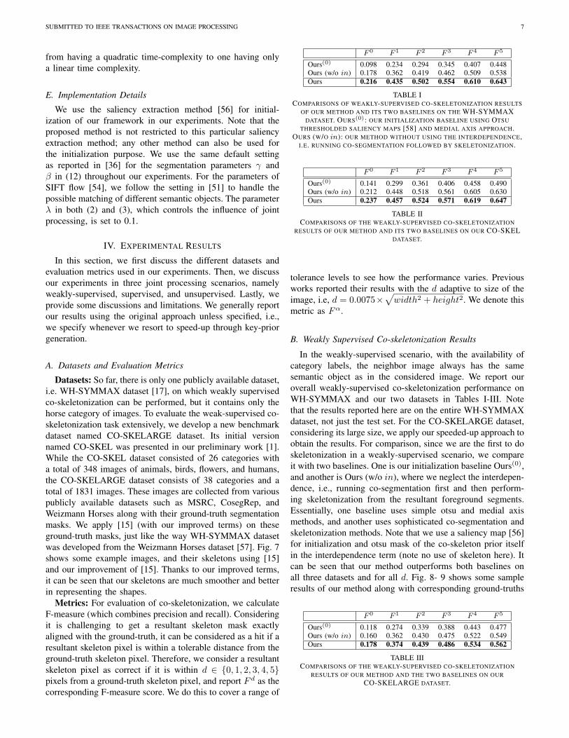
Metrics: For evaluation of co-skeletonization, we calculateF-measure (which combines precision and recall). Consideringit is challenging to get a resultant skeleton mask exactlyaligned with the ground-truth, it can be considered as a hit if aresultant skeleton pixel is within a tolerable distance from theground-truth skeleton pixel. Therefore, we consider a resultantskeleton pixel as correct if it is within d ∈ {0, 1, 2, 3, 4, 5}pixels from a ground-truth skeleton pixel, and report F d as thecorresponding F-measure score. We do this to cover a range of

F 0 F 1 F 2 F 3 F 4 F 5

Ours(0) 0.098 0.234 0.294 0.345 0.407 0.448Ours (w/o in) 0.178 0.362 0.419 0.462 0.509 0.538Ours 0.216 0.435 0.502 0.554 0.610 0.643

TABLE ICOMPARISONS OF WEAKLY-SUPERVISED CO-SKELETONIZATION RESULTS

OF OUR METHOD AND ITS TWO BASELINES ON THE WH-SYMMAXDATASET. OURS(0) : OUR INITIALIZATION BASELINE USING OTSU

THRESHOLDED SALIENCY MAPS [58] AND MEDIAL AXIS APPROACH.OURS (W/O in): OUR METHOD WITHOUT USING THE INTERDEPENDENCE,

I.E. RUNNING CO-SEGMENTATION FOLLOWED BY SKELETONIZATION.

F 0 F 1 F 2 F 3 F 4 F 5


TABLE IICOMPARISONS OF THE WEAKLY-SUPERVISED CO-SKELETONIZATION

RESULTS OF OUR METHOD AND ITS TWO BASELINES ON OUR CO-SKELDATASET.

tolerance levels to see how the performance varies. Previousworks reported their results with the d adaptive to size of theimage, i.e, d = 0.0075×

√width2 + height2. We denote this

metric as Fα.

B. Weakly Supervised Co-skeletonization Results

In the weakly-supervised scenario, with the availability ofcategory labels, the neighbor image always has the samesemantic object as in the considered image. We report ouroverall weakly-supervised co-skeletonization performance onWH-SYMMAX and our two datasets in Tables I-III. Notethat the results reported here are on the entire WH-SYMMAXdataset, not just the test set. For the CO-SKELARGE dataset,considering its large size, we apply our speeded-up approach toobtain the results. For comparison, since we are the first to doskeletonization in a weakly-supervised scenario, we compareit with two baselines. One is our initialization baseline Ours(0),and another is Ours (w/o in), where we neglect the interdepen-dence, i.e., running co-segmentation first and then perform-ing skeletonization from the resultant foreground segments.Essentially, one baseline uses simple otsu and medial axismethods, and another uses sophisticated co-segmentation andskeletonization methods. Note that we use a saliency map [56]for initialization and otsu mask of the co-skeleton prior itselfin the interdependence term (note no use of skeleton here). Itcan be seen that our method outperforms both baselines onall three datasets and for all d. Fig. 8- 9 shows some sampleresults of our method along with corresponding ground-truths

F 0 F 1 F 2 F 3 F 4 F 5


TABLE IIICOMPARISONS OF THE WEAKLY-SUPERVISED CO-SKELETONIZATION

RESULTS OF OUR METHOD AND THE TWO BASELINES ON OURCO-SKELARGE DATASET.


Image Simplicity Ours Image Simplicity Ours Image Simplicity Ours

Fig. 7. Given the shape, we improve skeletonization method Smplicity[15] using our improved terms in Simplicity[15]’s objective function. It can be seenthat our skeletons are much smoother and better in representing the shape.

Image Groundtruth Ours Image Groundtruth Ours Image Groundtruth Ours Image Groundtruth Ours

Fig. 8. Sample weakly-supervised co-skeletonization results on CO-SKEL dataset along with our final shape masks. It can be seen that both are quite closeto the groundtruths.

on our datasets. Also, we report results on individual categoriesof our two datasets in Tables IV-V. Low variances suggest thatour method is sufficiently reliable.

In Fig. 10, few samples are shown where the results im-prove iteration by iteration. To analyze this quantitatively, weevaluate the performance after every iteration in Fig. 11 on theWH-SYMMAX dataset. It can be seen that the performances,denoted by F 0 − F 5 and J (Jaccard Similarity for segmen-tation evaluation), improve after every iteration steadily andsynergistically. A choice of 2 to 3 iterations is good enoughfor our method to obtain reasonable performance.

C. Supervised Co-skeletonization Results

In the literature, there are numerous supervised skele-tonization methods available for comparison. As mentioned

earlier, while using the proposed method in the supervisedscenario, the training images are initialized with ground truths,and kNN is applied to find the nearest neighbors of testingimages from the training dataset. Such neighbors with ground-truths naturally boost the performance of co-skeletonizationfor developing useful priors of the test images. We make thecomparison with existing supervised skeletonization methodson test images of the WH-SYMMAX and SK506 datasetsin Table VI. We denote the co-skeletonization results of oursupervised approach as ”Ours (S)”, where we provide ground-truth skeleton annotations to the training images. Note thattheir segment masks can be easily computed from skeletonsusing grabcut through the enclosing bounding box. Our su-pervised approach outperforms the other supervised meth-ods convincingly. Note that we take the performance values


Image Groundtruth Ours Image Groundtruth Ours Image Groundtruth Ours Image Groundtruth Ours

Fig. 9. Sample weakly-supervised co-skeletonization results on CO-SKELARGE dataset along with our final shape masks. It can be seen that both are quiteclose to the groundtruths.


Fig. 10. Some examples of steadily improving skeletonization and segmentation after each iteration. The top-right example shows that our model continuesto reproduce similar results once the optimal shape and skeleton are obtained.

m F 0 F 1 F 2 F 3 F 4 F 5

bear 4 0.050 0.189 0.259 0.305 0.379 0.425camel 10 0.377 0.618 0.686 0.727 0.761 0.781cat 8 0.143 0.419 0.530 0.610 0.679 0.724cheetah 10 0.069 0.179 0.239 0.297 0.361 0.397cormorant 8 0.346 0.543 0.599 0.647 0.698 0.730cow 28 0.138 0.403 0.530 0.615 0.691 0.733cranesbill 7 0.240 0.576 0.658 0.706 0.748 0.774deer 6 0.279 0.465 0.522 0.577 0.649 0.683desertrose 15 0.329 0.675 0.755 0.800 0.838 0.857dog 11 0.133 0.410 0.504 0.573 0.637 0.670erget 14 0.405 0.626 0.665 0.696 0.723 0.742firepink 6 0.493 0.839 0.895 0.925 0.949 0.958frog 7 0.183 0.366 0.433 0.492 0.544 0.576germanium 17 0.295 0.614 0.697 0.750 0.801 0.828horse 31 0.273 0.491 0.551 0.599 0.651 0.683iris 10 0.358 0.637 0.703 0.746 0.790 0.808man 20 0.126 0.260 0.299 0.329 0.365 0.387ostrich 11 0.291 0.514 0.582 0.625 0.658 0.679panda 15 0.031 0.094 0.135 0.169 0.216 0.245pigeon 16 0.144 0.288 0.333 0.367 0.405 0.425seagull 13 0.180 0.336 0.397 0.448 0.500 0.530seastar 9 0.448 0.739 0.781 0.811 0.839 0.851sheep 10 0.115 0.342 0.465 0.535 0.608 0.650snowowl 10 0.130 0.281 0.325 0.362 0.421 0.457statue 29 0.301 0.525 0.571 0.599 0.623 0.642woman 23 0.276 0.451 0.500 0.536 0.572 0.596variance 0.016 0.034 0.034 0.034 0.032 0.030

TABLE IVCATEGORYWISE NUMBER OF IMAGES AND OUR WEAKLY-SUPERVISED

CO-SKELETONIZATION RESULTS ON THE CO-SKEL DATASET.

of other methods from [21]. We would like to point outthat the recently developed deep learning based supervisedmethods [21], [22] report better performance. However, werefrain from comparing with it for the following reasons:(i) The results that [21] reports are max-pooled resultsobtained from tuning over a wide range of thresholds. Incontrast, our results reported here are without any parametertuning. (ii) [21] takes extra help in the form of a pre-trained network, which they use to build upon, whereas werely on just saliency estimation. (iii) [21] uses both skeleton

m F 0 F 1 F 2 F 3 F 4 F 5

banana 7 0.122 0.358 0.422 0.469 0.528 0.564bear 24 0.134 0.332 0.413 0.479 0.541 0.572brush 6 0.102 0.317 0.419 0.496 0.551 0.574camel 12 0.300 0.501 0.555 0.592 0.634 0.662cat 42 0.118 0.333 0.421 0.483 0.546 0.582cheetah 10 0.067 0.200 0.265 0.322 0.387 0.425cormorant 8 0.370 0.577 0.612 0.633 0.660 0.684cow 87 0.121 0.344 0.445 0.509 0.572 0.609cranesbill 7 0.257 0.563 0.634 0.679 0.717 0.744deer 6 0.211 0.355 0.398 0.441 0.486 0.512desertrose 15 0.311 0.630 0.700 0.740 0.780 0.800dog 70 0.125 0.352 0.439 0.497 0.557 0.591eagle 9 0.168 0.489 0.582 0.648 0.722 0.757egret 14 0.420 0.633 0.666 0.694 0.726 0.743elephant 46 0.078 0.214 0.275 0.321 0.376 0.410firepink 6 0.422 0.721 0.784 0.833 0.888 0.911flowerwise 8 0.072 0.209 0.288 0.347 0.405 0.442frog 7 0.180 0.371 0.425 0.473 0.513 0.534geranium 17 0.285 0.600 0.691 0.743 0.791 0.819giraffe 213 0.100 0.277 0.346 0.392 0.442 0.470horse 245 0.143 0.348 0.419 0.467 0.520 0.552hydrant 62 0.151 0.360 0.459 0.520 0.572 0.605iris 10 0.351 0.634 0.702 0.743 0.787 0.805cutlery 6 0.055 0.149 0.207 0.257 0.303 0.331man 411 0.120 0.322 0.401 0.455 0.509 0.538ostrich 11 0.304 0.542 0.608 0.651 0.688 0.712panda 15 0.041 0.119 0.170 0.215 0.265 0.297parrot 5 0.040 0.143 0.214 0.282 0.348 0.378pigeon 19 0.124 0.255 0.299 0.331 0.361 0.382plane 169 0.202 0.496 0.593 0.648 0.702 0.732seagull 26 0.185 0.364 0.434 0.483 0.525 0.553seastar 9 0.407 0.654 0.686 0.708 0.735 0.749sheep 50 0.093 0.279 0.359 0.414 0.474 0.507snowowl 10 0.110 0.261 0.315 0.354 0.402 0.435statue 29 0.327 0.576 0.622 0.646 0.668 0.684swan 6 0.086 0.175 0.206 0.238 0.277 0.305woman 122 0.165 0.376 0.456 0.511 0.565 0.595zebra 12 0.131 0.344 0.430 0.497 0.563 0.597variance 0.013 0.027 0.026 0.025 0.024 0.024

TABLE VCATEGORYWISE NUMBER OF IMAGES AND OUR WEAKLY SUPERVISEDCO-SKELETONIZATION RESULTS ON THE CO-SKELARGE DATASET.


0

0.1

0.2

0.3

0.4

0.5

0.6

0.7

0.8

0 1 2 3

J

F5

F4

F3

F2

F1

F0

Fig. 11. Performance v/s Iteration plot. It can be seen that both the skele-tonization performance (denoted by F0-F5) and segmentation performance(denoted by J) improve after every iteration synergistically.

Methods WH-SYMMAX SK506 SK-LARGESymmetric [59] 0.174 0.218 0.243Deformable Disc [60] 0.223 0.252 0.255Particle Filter [61] 0.334 0.226 -Distance Regression [62] 0.103 - -MIL [16] 0.365 0.392 0.293MISL [33] 0.402 - -Ours (S) 0.618 0.525 0.501

TABLE VICOMPARISONS OF THE SUPERVISED CO-SKELETONIZATION RESULTS OFOUR METHOD WITH OTHER SUPERVISED METHODS USING Fα METRIC.

annotation and shape information annotation while training,whereas we use only skeleton annotations for training images.(iv) Essentially, our proposed method is a weakly-supervisedmethod or unsupervised method, with the possibility of addingstrong supervision, however, by replacing the saliency initial-ization with ground-truth skeleton initialization in the trainingdataset while extracting the neighbors. There is no traininginvolved as such in such this approach, meaning we are notlearning any parameters. In contrast, the existing methods aresupervised ones. To compare with them, we employ such amanner of supervision, and we can’t expect much boost in theperformance with this.

D. Unsupervised Co-skeletonization Results

The proposed method works in the unsupervised scenariotoo, where absolutely no annotations are provided. The pro-posed method under this scenario completely relies on theclustering process to retrieve suitable neighbors in a mixedimage collection. Since SK-506 and SK-LARGE datasets aresuitable for this purpose, we report our unsupervised co-skeletonization results in Table VII on these datasets whilecomparing with the two baselines. Note that these unsu-pervised results are on the entire dataset, not just the testpart. In the unsupervised scenario as well proposed methodoutperforms the two baselines. Note that since SK-LARGE isa large dataset, we apply our key prior propagation approach.

SK-506 SK-LARGEOurs0 0.362 0.333Ours (w/o in) 0.365 0.352Ours 0.475 0.429

TABLE VIICOMPARISONS OF THE UNSUPERVISED CO-SKELETONIZATION RESULTS

OF OUR METHOD WITH THE TWO BASELINES USING Fα METRIC.

Run-time (in mins) PerformanceOriginal 230 0.545Key Prior Propagation 80 0.532

TABLE VIIICOMPARISON OF OUR TWO APPROACHES IN TERMS OF THE RUN-TIME

AND THE PERFORMANCE ON WH-SYMMAX DATASET. WHILE THERE ISA SPEED-UP OF ALMOST THREE TIMES, THE DROP IN PERFORMANCE ISMARGINAL. NOTE THAT THE TIME REPORTED IS THE TIME TAKEN FOR

PRIOR GENERATION, NOT THE ENTIRE TIME.

E. Original approach v/s Key Prior Propagation approach

The main difference between our original key prior propa-gation approach is the way our two priors, co-skeleton priorand co-segment prior, are generated. The latter requires asignificantly lesser number of alignments compared to the firstat the cost of an assumption that the alignments are precise. InTable VIII, we show how significant is the speed up and dropin the performance when both the approaches are applied tothe WH-SYMMAX dataset. While there is a speed-up of threetimes, the drop in the performance is just marginal. Therefore,the assumption holds to a good degree.

F. Discussions and Limitations

We show few sampled segmentation results initialized bypoor saliency map [58] in Fig. 12. Despite such poor initial-izations, our algorithm manages to segment out the objectsconvincingly well, thanks to joint processing. Our method hassome limitations. First, for initialization, our method requirescommon object parts to be salient in general across theneighboring images, if not in all. Therefore, it depends onthe quality of the neighbor images. The second limitationlies in difficulty during the warping process. For example,

Image Saliency Our Result Image Saliency Our Result

Fig. 12. Good segmentation examples despite the bad saliency maps


when the neighboring images contain objects at different sizesor from different viewpoints, the warping processing finds itchallenging to align the images well. However, such a situationis unlikely to occur when there are a large number of images,resulting in diversity to select appropriate neighbors. Anotherissue is that smoothing the skeleton may cause missing outsome essential short branches. The third limitation occurswhen a part occludes other parts of the object. As a result,the shape of the object doesn’t look desirable for properlyskeletonizing the objects. For example, a baseball player inFig. 9 misses out his left hand.

V. CONCLUSION

The major contributions of this paper lie in our novelobject co-skeletonization problem and the proposed coupledco-skeletonization and co-segmentation framework, which ef-fectively exploits inherent interdependencies between the twoto assist each other synergistically. Extensive experimentsdemonstrate that the proposed method achieves very competi-tive results on different benchmark datasets, including our newCO-SKELARGE dataset, developed especially for weakly-supervised co-skeletonization benchmarking.

ACKNOWLEDGMENT

This research is supported by the National Research Foun-dation, Prime Minister’s Office, Singapore, under its IDMFutures Funding Initiative. It is also supported by the HCCSresearch grant at the ADSC1 from Singapore’s A*STAR.

REFERENCES

[1] K. R. Jerripothula, J. Cai, J. Lu, and J. Yuan, “Object co-skeletonizationwith co-segmentation,” in 2017 IEEE Conference on Computer Visionand Pattern Recognition (CVPR), July 2017, pp. 3881–3889.

[2] C. Rother, T. Minka, A. Blake, and V. Kolmogorov, “Cosegmentationof image pairs by histogram matching-incorporating a global constraintinto mrfs,” in Computer Vision and Pattern Recognition(CVPR). IEEE,2006, pp. 993–1000.

[3] H. Wang, Y. Lai, W. Cheng, C. Cheng, and K. Hua, “Backgroundextraction based on joint gaussian conditional random fields,” IEEETransactions on Circuits and Systems for Video Technology, vol. 28,no. 11, pp. 3127–3140, Nov 2018.

[4] K. R. Jerripothula, J. Cai, and J. Yuan, “Cats: Co-saliency activatedtracklet selection for video co-localization,” in European Conference onComputer vision (ECCV). Springer, 2016, pp. 187–202.

[5] W. Wang, J. Shen, H. Sun, and L. Shao, “Video co-saliency guided co-segmentation,” IEEE Transactions on Circuits and Systems for VideoTechnology, vol. 28, no. 8, pp. 1727–1736, Aug 2018.

[6] H. Zhu, F. Meng, J. Cai, and S. Lu, “Beyond pixels: A comprehensivesurvey from bottom-up to semantic image segmentation and cosegmen-tation,” Journal of Visual Communication and Image Representation(JVCIR), vol. 34, pp. 12 – 27, 2016.

[7] K. R. Jerripothula, J. Cai, and J. Yuan, “Qcce: Quality constrained co-saliency estimation for common object detection,” in Visual Communi-cations and Image Processing (VCIP). IEEE, 2015, pp. 1–4.

[8] F. Meng, J. Cai, and H. Li, “Cosegmentation of multiple image groups,”Computer Vision and Image Understanding (CVIU), vol. 146, pp. 67 –76, 2016.

[9] K. R. Jerripothula, J. Cai, and J. Yuan, “Efficient video object co-localization with co-saliency activated tracklets,” IEEE Transactions onCircuits and Systems for Video Technology, vol. 29, no. 3, pp. 744–755,March 2019.

1This work was partly done when Koteswar and Jiangbo were interningand working in ADSC

[10] F. Wang, Q. Huang, and L. J. Guibas, “Image co-segmentation viaconsistent functional maps,” in 2013 IEEE International Conference onComputer Vision, Dec 2013, pp. 849–856.

[11] K. Chang, T. Liu, and S. Lai, “From co-saliency to co-segmentation: Anefficient and fully unsupervised energy minimization model,” in CVPR2011, June 2011, pp. 2129–2136.

[12] K. R. Jerripothula, “Co-saliency based visual object co-segmentation andco-localization,” Ph.D. dissertation, Nanyang Technological University(NTU), 2017.

[13] Z. Yu, J. Yu, C. Xiang, Z. Zhao, Q. Tian, and D. Tao, “Rethinkingdiversified and discriminative proposal generation for visual grounding,”in Proceedings of the 27th International Joint Conference on ArtificialIntelligence, ser. IJCAI’18. AAAI Press, 2018, pp. 1114–1120.[Online]. Available: http://dl.acm.org/citation.cfm?id=3304415.3304573

[14] W.-P. Choi, K.-M. Lam, and W.-C. Siu, “Extraction of the euclideanskeleton based on a connectivity criterion,” Pattern Recognition, vol. 36,no. 3, pp. 721 – 729, 2003.

[15] W. Shen, X. Bai, X. Yang, and L. J. Latecki, “Skeleton pruning as trade-off between skeleton simplicity and reconstruction error,” Science ChinaInformation Sciences, vol. 56, no. 4, pp. 1–14, 2013.

[16] S. Tsogkas and I. Kokkinos, “Learning-based symmetry detection innatural images,” in European Conference on Computer Vision (ECCV).Springer Berlin Heidelberg, 2012, pp. 41–54.

[17] W. Shen, X. Bai, Z. Hu, and Z. Zhang, “Multiple instance subspacelearning via partial random projection tree for local reflection symmetryin natural images,” Pattern Recognition, vol. 52, pp. 306 – 316, 2016.

[18] J. Yu, C. Zhu, J. Zhang, Q. Huang, and D. Tao, “Spatial pyramid-enhanced netvlad with weighted triplet loss for place recognition,” IEEETransactions on Neural Networks and Learning Systems, pp. 1–14, 2019.

[19] J. Yu, B. Zhang, Z. Kuang, D. Lin, and J. Fan, “iprivacy: Image privacyprotection by identifying sensitive objects via deep multi-task learning,”IEEE Transactions on Information Forensics and Security, vol. 12, no. 5,pp. 1005–1016, May 2017.

[20] J. Yu, X. Yang, F. Gao, and D. Tao, “Deep multimodal distance metriclearning using click constraints for image ranking,” IEEE Transactionson Cybernetics, vol. 47, no. 12, pp. 4014–4024, Dec 2017.

[21] W. Shen, K. Zhao, Y. Jiang, Y. Wang, Z. Zhang, and X. Bai, “Objectskeleton extraction in natural images by fusing scale-associated deep sideoutputs,” in Computer Vision and Pattern Recognition (CVPR). IEEE,2016, pp. 222–230.

[22] W. Shen, K. Zhao, Y. Jiang, Y. Wang, X. Bai, and A. Yuille, “Deepskele-ton: Learning multi-task scale-associated deep side outputs for objectskeleton extraction in natural images,” IEEE Transactions on ImageProcessing, vol. 26, no. 11, pp. 5298–5311, 2017.

[23] S. Xie and Z. Tu, “Holistically-nested edge detection,” in InternationalConference on Computer Vision (ICCV). IEEE, 2015, pp. 1395–1403.

[24] J. Zhang, J. Yu, and D. Tao, “Local deep-feature alignment for unsuper-vised dimension reduction,” IEEE Transactions on Image Processing,vol. 27, no. 5, pp. 2420–2432, May 2018.

[25] L.-C. Chen, G. Papandreou, I. Kokkinos, K. Murphy, and A. L. Yuille,“Semantic image segmentation with deep convolutional nets and fullyconnected crfs,” arXiv preprint arXiv:1412.7062, 2014.

[26] K. He, G. Gkioxari, P. Dollar, and R. Girshick, “Mask r-cnn,” inProceedings of the IEEE international conference on computer vision,2017, pp. 2961–2969.

[27] J. Guo, L. Cheong, and R. Tan, “Video foreground cosegmentation basedon common fate,” IEEE Transactions on Circuits and Systems for VideoTechnology, vol. 28, no. 3, pp. 586–600, March 2018.

[28] K. R. Jerripothula, J. Cai, F. Meng, and J. Yuan, “Automatic imageco-segmentation using geometric mean saliency,” in International Con-ference on Image Processing (ICIP). IEEE, 2014, pp. 3282–3286.

[29] K. R. Jerripothula, J. Cai, and J. Yuan, “Quality-guided fusion-basedco-saliency estimation for image co-segmentation and colocalization,”IEEE Transactions on Multimedia, vol. 20, no. 9, pp. 2466–2477, Sep.2018.

[30] P. K. Saha, G. Borgefors, and G. S. di Baja, “A survey on skeletonizationalgorithms and their applications,” Pattern Recognition Letters, vol. 76,pp. 3 – 12, 2016, special Issue on Skeletonization and its Application.

[31] W. Shen, X. Bai, R. Hu, H. Wang, and L. J. Latecki, “Skeleton growingand pruning with bending potential ratio,” Pattern Recognition, vol. 44,no. 2, pp. 196 – 209, 2011.

[32] Z. Yu and C. Bajaj, “A segmentation-free approach for skeletonization ofgray-scale images via anisotropic vector diffusion,” in Computer Visionand Pattern Recognition (CVPR). IEEE, 2004, pp. 415 – 420.

[33] Q. Zhang and I. Couloigner, “Accurate centerline detection and linewidth estimation of thick lines using the radon transform,” IEEE

http://dl.acm.org/citation.cfm?id=3304415.3304573


Transactions on Image Processing (T-IP), vol. 16, no. 2, pp. 310–316,2007.

[34] T. Lindeberg, “Edge detection and ridge detection with automatic scaleselection,” International Journal of Computer Vision, vol. 30, no. 2, pp.117–156, 1998.

[35] S. Ren, K. He, R. Girshick, and J. Sun, “Faster r-cnn: Towards real-timeobject detection with region proposal networks,” IEEE Transactions onPattern Analysis and Machine Intelligence, vol. 39, no. 6, pp. 1137–1149, June 2017.

[36] C. Rother, V. Kolmogorov, and A. Blake, “Grabcut: Interactive fore-ground extraction using iterated graph cuts,” in Transactions on Graphics(TOG), vol. 23, no. 3. ACM, 2004, pp. 309–314.

[37] M. Tang, L. Gorelick, O. Veksler, and Y. Boykov, “Grabcut in onecut,” in International Conference on Computer Vision (ICCV), 2013,pp. 1769–1776.

[38] K. R. Jerripothula, J. Cai, and J. Yuan, “Image co-segmentation viasaliency co-fusion,” IEEE Transactions on Multimedia (T-MM), vol. 18,no. 9, pp. 1896–1909, Sept 2016.

[39] J. Dai, Y. N. Wu, J. Zhou, and S.-C. Zhu, “Cosegmentation and cosketchby unsupervised learning,” in International Conference on ComputerVision (ICCV). IEEE, 2013.

[40] K. R. Jerripothula, J. Cai, and J. Yuan, “Group saliency propagationfor large scale and quick image co-segmentation,” in InternationalConference on Image Processing (ICIP). IEEE, 2015, pp. 4639–4643.

[41] E. Shelhamer, J. Long, and T. Darrell, “Fully convolutional networksfor semantic segmentation,” IEEE Transactions on Pattern Analysis andMachine Intelligence (T-PAMI), vol. 39, no. 4, pp. 640–651, 2017.

[42] D. Lin, J. Dai, J. Jia, K. He, and J. Sun, “Scribblesup: Scribble-supervised convolutional networks for semantic segmentation,” in TheIEEE Conference on Computer Vision and Pattern Recognition (CVPR).IEEE, 2016.

[43] D. Batra, A. Kowdle, D. Parikh, J. Luo, and T. Chen, “icoseg: Interactiveco-segmentation with intelligent scribble guidance,” in Computer Visionand Pattern Recognition (CVPR). IEEE, 2010, pp. 3169–3176.

[44] D. S. Hochbaum and V. Singh, “An efficient algorithm for co-segmentation,” in International Conference on Computer Vision (ICCV).IEEE, 2009, pp. 269–276.

[45] A. Joulin, F. Bach, and J. Ponce, “Discriminative clustering for imageco-segmentation,” in Computer Vision and Pattern Recognition (CVPR).IEEE, 2010, pp. 1943–1950.

[46] L. Mukherjee, V. Singh, and C. R. Dyer, “Half-integrality based algo-rithms for cosegmentation of images,” in Computer Vision and PatternRecognition (CVPR). IEEE, 2009, pp. 2028–2035.

[47] J. Yuan, G. Zhao, Y. Fu, Z. Li, A. K. Katsaggelos, and Y. Wu,“Discovering thematic objects in image collections and videos,” IEEETransactions on Image Processing (T-IP), vol. 21, no. 4, pp. 2207–2219,2012.

[48] G. Zhao and J. Yuan, “Mining and cropping common objects fromimages,” in ACM Multimedia (MM). ACM, 2010, pp. 975–978.

[49] G. Kim, E. P. Xing, L. Fei-Fei, and T. Kanade, “Distributed coseg-mentation via submodular optimization on anisotropic diffusion,” inInternational Conference on Computer Vision (ICCV). IEEE, 2011,pp. 169–176.

[50] A. Joulin, F. Bach, and J. Ponce, “Multi-class cosegmentation,” inComputer Vision and Pattern Recognition (CVPR). IEEE, 2012, pp.542–549.

[51] M. Rubinstein, A. Joulin, J. Kopf, and C. Liu, “Unsupervised joint objectdiscovery and segmentation in internet images,” in Computer Vision andPattern Recognition (CVPR). IEEE, 2013, pp. 1939–1946.

[52] A. Faktor and M. Irani, “Co-segmentation by composition,” in Inter-national Conference on Computer Vision (ICCV). IEEE, 2013, pp.1297–1304.

[53] R. Cong, J. Lei, H. Fu, M. Cheng, W. Lin, and Q. Huang, “Reviewof visual saliency detection with comprehensive information,” IEEETransactions on Circuits and Systems for Video Technology, pp. 1–1,2018.

[54] C. Liu, J. Yuen, and A. Torralba, “Sift flow: Dense correspondenceacross scenes and its applications,” IEEE Transactions on PatternAnalysis and Machine Intelligence (T-PAMI), vol. 33, no. 5, pp. 978–994, 2011.

[55] A. Oliva and A. Torralba, “Modeling the shape of the scene: A holisticrepresentation of the spatial envelope,” International journal of computervision (IJCV), vol. 42, no. 3, pp. 145–175, 2001.

[56] W. Zhu, S. Liang, Y. Wei, and J. Sun, “Saliency optimization from robustbackground detection,” in 2014 IEEE Conference on Computer Visionand Pattern Recognition, June 2014, pp. 2814–2821.

[57] E. Borenstein and S. Ullman, “Class-specific, top-down segmentation,”in European Conference on Computer Vision (ECCV). Springer BerlinHeidelberg, 2002, pp. 109–122.

[58] M.-M. Cheng, G.-X. Zhang, N. J. Mitra, X. Huang, and S.-M. Hu,“Global contrast based salient region detection,” in Computer Visionand Pattern Recognition (CVPR). IEEE, 2011, pp. 409–416.

[59] A. Levinshtein, S. Dickinson, and C. Sminchisescu, “Multiscale sym-metric part detection and grouping,” in International Conference onComputer Vision (ICCV). IEEE, 2009, pp. 2162–2169.

[60] T. S. H. Lee, S. Fidler, and S. Dickinson, “Detecting curved symmetricparts using a deformable disc model,” in International Conference onComputer Vision (ICCV). IEEE, 2013, pp. 1753–1760.

[61] N. Widynski, A. Moevus, and M. Mignotte, “Local symmetry detectionin natural images using a particle filtering approach,” IEEE Transactionson Image Processing (T-IP), vol. 23, no. 12, pp. 5309–5322, 2014.

[62] A. Sironi, V. Lepetit, and P. Fua, “Multiscale centerline detection bylearning a scale-space distance transform,” in Computer Vision andPattern Recognition (CVPR). IEEE, 2014, pp. 2697–2704.

submitted to ieee transactions on image processing 1 …

Documents