AQR Capital Management, LLC

Two Greenwich Plaza

Greenwich, CT 06830

p: +1.203.742.3600 | w: aqr.com

Style Premia: Environments, Timing, Crowding

Principal

Antti Ilmanen

1

Nomura, 10th Annual Global Quantitative Investment Strategies Conference

June 9, 2016

AQR Color

Palette

AQR Cyan

Auxiliary Palette

Disclosures

2

The information set forth herein has been obtained or derived from sources believed by AQR Capital Management, LLC (“AQR”) to be reliable. However, AQR does not make any

representation or warranty, express or implied, as to the information’s accuracy or completeness, nor does AQR recommend that the attached information serve as the basis of

any investment decision. This document has been provided to you solely for information purposes and does not constitute an offer or solicitation of an offer, or any advice or

recommendation, to purchase any securities or other financial instruments, and may not be construed as such. This document is intended exclusively for the use of the person to

whom it has been delivered by AQR and it is not to be reproduced or redistributed to any other person. Please refer to the Appendix for more information on risks and fees. For

one-on-one presentation use only. Past performance is not a guarantee of future performance.

This presentation is not research and should not be treated as research. This presentation does not represent valuation judgments with respect to any financial instrument, issuer, security or sector that may be described or referenced herein and does not represent a formal or official view of AQR.

The views expressed reflect the current views as of the date hereof and neither the speaker nor AQR undertakes to advise you of any changes in the views expressed herein. It should not be assumed that the speaker or AQR will make investment recommendations in the future that are consistent with the views expressed herein, or use any or all of the techniques or methods of analysis described herein in managing client accounts. AQR and its affiliates may have positions (long or short) or engage in securities transactions that are not consistent with the information and views expressed in this presentation.

The information contained herein is only as current as of the date indicated, and may be superseded by subsequent market events or for other reasons. Charts and graphs provided herein are for illustrative purposes only. The information in this presentation has been developed internally and/or obtained from sources believed to be reliable; however, neither AQR nor the speaker guarantees the accuracy, adequacy or completeness of such information. Nothing contained herein constitutes investment, legal, tax or other advice nor is it to be relied on in making an investment or other decision.

There can be no assurance that an investment strategy will be successful. Historic market trends are not reliable indicators of actual future market behavior or future performance of any particular investment which may differ materially, and should not be relied upon as such. Target allocations contained herein are subject to change. There is no assurance that the target allocations will be achieved, and actual allocations may be significantly different than that shown here. This presentation should not be viewed as a current or past recommendation or a solicitation of an offer to buy or sell any securities or to adopt any investment strategy.

The information in this presentation may contain projections or other forward‐looking statements regarding future events, targets, forecasts or expectations regarding the strategies described herein, and is only current as of the date indicated. There is no assurance that such events or targets will be achieved, and may be significantly different from that shown here. The information in this presentation, including statements concerning financial market trends, is based on current market conditions, which will fluctuate and may be superseded by subsequent market events or for other reasons. Performance of all cited indices is calculated on a total return basis with dividends reinvested.

The investment strategy and themes discussed herein may be unsuitable for investors depending on their specific investment objectives and financial situation. Please note that changes in the rate of exchange of a currency may affect the value, price or income of an investment adversely.

Neither AQR nor the speaker assumes any duty to, nor undertakes to update forward looking statements. No representation or warranty, express or implied, is made or given by or on behalf of AQR, the speaker or any other person as to the accuracy and completeness or fairness of the information contained in this presentation, and no responsibility or liability is accepted for any such information. By accepting this presentation in its entirety, the recipient acknowledges its understanding and acceptance of the foregoing statement.

Introduction to Major Style Premia - Value, Momentum, Carry, Defensive, Trend - Applied in Many Asset Classes - Long-Run Evidence and Qualifiers

Introduction to Styles

4

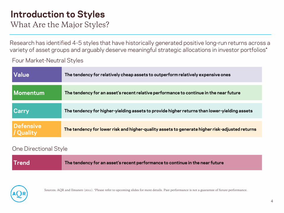
Momentum The tendency for an asset’s recent relative performance to continue in the near future

Value The tendency for relatively cheap assets to outperform relatively expensive ones

Carry The tendency for higher-yielding assets to provide higher returns than lower-yielding assets

Defensive / Quality

The tendency for lower risk and higher-quality assets to generate higher risk-adjusted returns

What Are the Major Styles?

Research has identified 4-5 styles that have historically generated positive long-run returns across a

variety of asset groups and arguably deserve meaningful strategic allocations in investor portfolios*

Four Market-Neutral Styles

Sources: AQR and Ilmanen (2011). *Please refer to upcoming slides for more details. Past performance is not a guarantee of future performance.

One Directional Style

Trend The tendency for an asset’s recent performance to continue in the near future

-0.5

0.0

0.5

1.0

1.5

2.0

2.5

Stocks & Industries Equity Indices Fixed Income Currencies Commodities Style Composite

Sh

arp

e R

ati

o

Value Momentum Carry Defensive

Asset GroupComposite

Sto

ck

s &

In

du

str

ies

EQ

In

dic

es

Fix

ed

In

co

me

Cu

rre

nc

ies

Co

mm

od

itie

s

Evidence Across Many Asset Groups and Styles

5

Single Long/Short Style Premia and Diversified Composites

Source: AQR. Above analysis reflects a backtest of theoretical long/short style components based on AQR definitions across identified asset

groups, and is for illustrative purposes only and not based on an actual portfolio AQR manages. The results shown do not include advisory

fees or transaction costs; if such fees and expenses were deducted the Sharpe ratios would be lower; returns are excess of cash. Please read

performance disclosures in the Appendix for a description of the investment universe and the allocation methodology used to construct the

backtest and composites. Hypothetical data has inherent limitations, some of which are disclosed in the Appendix.

Hypothetical Gross Sharpe Ratios of Long/Short Style Components Across Asset Groups

January 1990 – December 2015

N/A N/A N/A N/A

Single long/short strategies performed well…

Composites may be even better

Qualifiers: What Are Realistic Expectations For the Future?

No matter how stringent our criteria, history may overstate future results

• It is important to adjust historical backtest returns for costs and fees

• The magnitude of returns from known style premia may well be smaller going forward; we often

assume half or less of historical rewards – either due to overfitting or overcrowding concerns

Still, diversification helps boost portfolio Sharpe ratio, especially in market-neutral applications

Thus a diversified portfolio of these strategies may be less reliant on the standalone efficacy of

any one style in any one asset class – but very reliant on efficient execution as we magnify small

edges

To convert a Sharpe ratio advantage into high returns, some leverage will often be needed

6

Skepticism On Past Success Repeating…Is Partly Warranted

Source: AQR. Diversification does not eliminate the risk of experiencing investment losses. Please read important disclosures in the

Appendix.

Style Premia Across Environments – Robust performance across environments, so far – Contemporaneous relations do not imply predictability

Performance Across Growth and Inflation Environments

8

Macro Diversification: Mapping Investments to Macro Risks

Sources: Bloomberg, Cambridge Associates and AQR. Data from January 1972 – December 2014. The risk-free rate used in Sharpe ratio calculations is the Merrill Lynch 3 Month Treasury Bill

Index. Global Equities is the MSCI World Index. Global Bonds is a GDP weighted composite of Australian, German, Canadian, Japanese, U.K. and U.S. 10-year government bonds. Commodities

is an equal dollar-weighted index of 24 commodities. Private Equity and Real Estate are represented by Cambridge Associates indices. Long-Short Style Premia are backtests of style premia as

described herein. Global 60/40 is 60% Global Equities and 40% Global Bonds. Simplified Global Risk Parity is an equal risk allocation to Global Equities, Global Bonds and Commodities. Five

Styles is an equal dollar-weighted composite of the five long/short style premia. Please see the Appendix for more details on the construction of the return series and macroeconomic

environmental indicators. The analysis is based on hypothetical returns gross of trading costs and fees. Hypothetical performance results have certain inherent limitations, some of which are

disclosed in the Appendix. Past performance is not a guarantee of future performance. This information is supplemental to the GIPS® compliant presentation for the Style Premia Composite

incepted on 9/1/2012 in the Appendix.

Long-Only Market Risk Premia 1972-2014

Hypothetical Long/Short Style Premia 1972-2014

Hypothetical Simple Portfolios 1972-2014

Hypothetical Performance in Equity Market Tail Quarters

9

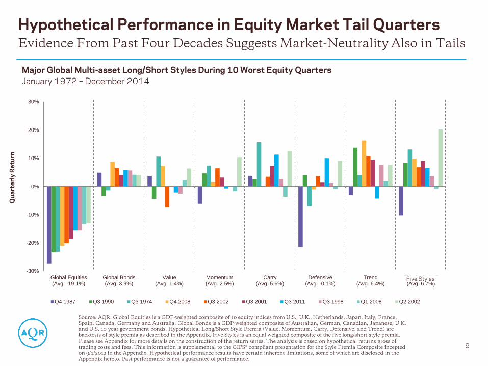
Evidence From Past Four Decades Suggests Market-Neutrality Also in Tails

Major Global Multi-asset Long/Short Styles During 10 Worst Equity Quarters

January 1972 – December 2014

Source: AQR. Global Equities is a GDP-weighted composite of 10 equity indices from U.S., U.K., Netherlands, Japan, Italy, France,

Spain, Canada, Germany and Australia. Global Bonds is a GDP-weighted composite of Australian, German, Canadian, Japanese, U.K.

and U.S. 10-year government bonds. Hypothetical Long/Short Style Premia (Value, Momentum, Carry, Defensive, and Trend) are

backtests of style premia as described in the Appendix. Five Styles is an equal weighted composite of the five long/short style premia.

Please see Appendix for more details on the construction of the return series. The analysis is based on hypothetical returns gross of

trading costs and fees. This information is supplemental to the GIPS® compliant presentation for the Style Premia Composite incepted

on 9/1/2012 in the Appendix. Hypothetical performance results have certain inherent limitations, some of which are disclosed in the

Appendix hereto. Past performance is not a guarantee of performance.

-30%

-20%

-10%

0%

10%

20%

30%

Global Equities(Avg. -19.1%)

Global Bonds(Avg. 3.9%)

Value(Avg. 1.4%)

Momentum(Avg. 2.5%)

Carry(Avg. 5.6%)

Defensive(Avg. -0.1%)

Trend(Avg. 6.4%)

Simple Style-5(Avg. 6.7%)

Q4 1987 Q3 1990 Q3 1974 Q4 2008 Q3 2002 Q3 2001 Q3 2011 Q3 1998 Q1 2008 Q2 2002

Qu

art

erl

y R

etu

rn

Five Styles

-40%

-30%

-20%

-10%

0%

10%

20%

30%

40%

Global Equities Global Bonds Commodities (Eq-wtd)

Hypothetical Performance When Real Yields Rise Sharply

10

Combination of Styles Has Held Up Well in Rising Real Yield Episodes

Cu

mu

lati

ve

Ex

ce

ss

Re

turn

-40%

-30%

-20%

-10%

0%

10 %

20 %

30 %

40 %

Global Equit ies Global Bonds Commodit ies (Eq-wt d)

12 /19 74 -09 /19 75 06 /19 79 -02 /19 80 06 /19 80 -09 /19 81 02 /19 83 -06 /19 84 08 /19 86 -09 /19 87

08 /19 93 -11 /19 94 09 /19 98 -01 /20 00 06 /20 05 -06 /20 06 12 /20 08 -12 /20 09 06 /20 12 -12 /20 13

Exc

ess R

etu

rn

-40%

-30%

-20%

-10%

0%

10%

20%

30%

40%

Global 60/40 Simple Global RiskParity

Simple Style-5

Source: AQR. See Alternative Thinking, October 2013, or the AQR white paper Exploring Macroeconomic Sensitivities (2013) for details of how these strategies

are constructed. Briefly, Global Equities is the MSCI World index net dividends. Global Bonds is a GDP-weighted composite of Australian, German, Canadian,

Japanese, U.K. and U.S. 10-year government bonds. Commodities is an equal-dollar-weighted index of 24 commodity futures. Global 60/40 takes 60% Global

Equities and 40% Global Bonds. Simple Global Risk Parity uses trailing 12-month volatility and long-term correlation assumptions to target equal risk-

contributions from a portfolio of Global Equities, Global Bonds and Commodities. Five Styles is an equal-weighted composite of five long/short style premia

(value, momentum, carry, defensive, trend) harvested in many asset classes. Details for Value, Momentum, Carry, Defensive, and Trend can be found in the

Appendix. The analysis is based on hypothetical returns gross of trading costs and fees. Hypothetical data has certain inherent limitations, some of which are

disclosed in the Appendix hereto. Past performance is not a guarantee of future performance.

Five Styles

Equity Market Correlations Are Low But Time-Varying

11

Source: AQR, Bloomberg, Ken French Data Library. Equities is the MSCI World Index. SMB (Size) returns sourced from “Portfolios

Formed on Size.” HML (Value) returns sourced from “Portfolios Formed on Book-to-Market.” UMD (Momentum) returns sourced from

“10 Portfolios Formed on Momentum.” See Kenneth R. French Data Library for further details. QMJ (Quality) is an updated and

extended version of the data used in the AQR paper “Quality Minus Junk” (Asness, Frazzini and Pedersen, 2014). BAB (Low Beta) is an

updated and extended version of the data used in the AQR paper “Betting Against Beta” (Frazzini and Pedersen, 2013). Return series

begin at different times based on earliest availability of data. Please read performance disclosures in the Appendix for a description of

the investment universe and the allocation methodology used to construct the backtests. Hypothetical data has inherent limitations,

some of which are disclosed in the Appendix.

-1.0

-0.5

0.0

0.5

1.0

1976 1981 1986 1991 1996 2001 2006 2011

Value

Momentum

Carry

Defensive

Trend

-1.0

-0.5

0.0

0.5

1.0

1990 1995 2000 2005 2010 2015

HML

UMD

SMB

BAB

QMJ

Rolling 60 Month Correlations to Equities — Hypothetical AQR Styles

January 1972 – March 2016

Rolling 60 Month Correlations to Equities — Academic Factors

January 1986 – March 2016

Style/Factor Timing Opportunities – and Crowding Concerns

AQR Color

Palette

AQR Cyan

Auxiliary Palette

-4

-3

-2

-1

0

1

2

3

4

1990 1995 2000 2005 2010 2015

Sta

nd

ard

ize

d V

alu

e S

pre

ad

Value

Momentum

Defensive

All Styles

Style Premia Valuations May Be Useful Crowding Indicators

13

But So Far Show No Red Light: More Oscillations than Downtrends

Source: AQR. Value spreads are calculated for long/short style portfolios using several different valuation measures. The top graph

shows a standardized weighted average of spreads in U.S., Japan, Europe and U.K stocks. The bottom graph shows a standardized

weighted average of spreads in equity country allocation, bonds, interest rate futures, currencies and commodities. This does not reflect

a portfolio that AQR currently manages and is for illustrative purposes only. Please see the appendix for a construction of the portfolios.

Hypothetical data has inherent limitations, some of which are disclosed in the Appendix hereto. Past performance is not a guarantee of

future performance.

-4

-3

-2

-1

0

1

2

3

4

1990 1995 2000 2005 2010 2015

Sta

nd

ard

ize

d V

alu

e S

pre

ad

Value

Momentum

Carry

Defensive

All Styles

Asset Allocation Style Premia Value Spreads Jan-1990 – Jan-2016

Cheap

Expensive

Stock Selection Style Premia Value Spreads Jan-1990 – Jan-2016

Cheap

Expensive

AQR Color

Palette

AQR Cyan

Auxiliary Palette

Static Timed

DIFF Value

Spreads

RATIO Value

Spreads

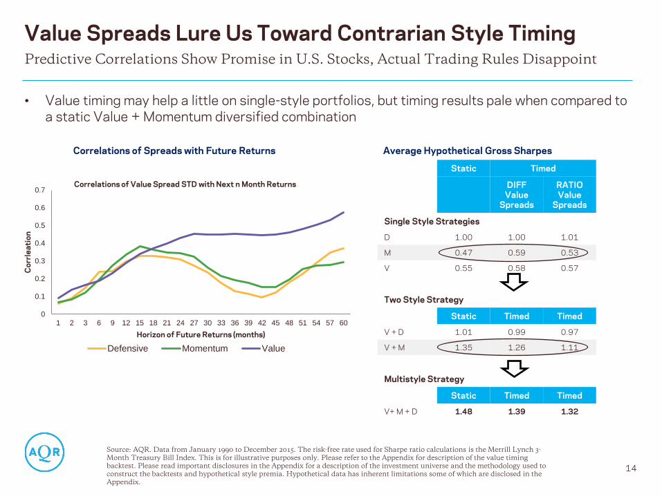
Single Style Strategies

D 1.00 1.00 1.01

M 0.47 0.59 0.53

V 0.55 0.58 0.57

Two Style Strategy

Static Timed Timed

V + D 1.01 0.99 0.97

V + M 1.35 1.26 1.11

Multistyle Strategy

Static Timed Timed

V+ M + D 1.48 1.39 1.32

Value Spreads Lure Us Toward Contrarian Style Timing

14

Predictive Correlations Show Promise in U.S. Stocks, Actual Trading Rules Disappoint

Source: AQR. Data from January 1990 to December 2015. The risk-free rate used for Sharpe ratio calculations is the Merrill Lynch 3-

Month Treasury Bill Index. This is for illustrative purposes only. Please refer to the Appendix for description of the value timing

backtest. Please read important disclosures in the Appendix for a description of the investment universe and the methodology used to

construct the backtests and hypothetical style premia. Hypothetical data has inherent limitations some of which are disclosed in the

Appendix.

• Value timing may help a little on single-style portfolios, but timing results pale when compared to

a static Value + Momentum diversified combination

Correlations of Spreads with Future Returns Average Hypothetical Gross Sharpes

0

0.1

0.2

0.3

0.4

0.5

0.6

0.7

1 2 3 6 9 12 15 18 21 24 27 30 33 36 39 42 45 48 51 54 57 60

Co

rrle

ati

on

Horizon of Future Returns (months)

Correlations of Value Spread STD with Next n Month Returns

Defensive Momentum Value

AQR Color

Palette

AQR Cyan

Auxiliary Palette

Same Story in Many Assets: Contrarian Timing Does Not Help

15

And Strategic Multi-Style Diversification Gives a High Bar to Beat

* Hit Rate defined as the percentage of strategies where timing improves gross Sharpe. V/M/C/D stand for Value, Momentum, Carry, and Defensive styles.

Source: AQR. Backtest from January 1995 to December 2015. The risk-free rate used in Sharpe ratio calculations is the Merrill Lynch 3 Month Treasury

Bill Index. These are not the returns of an actual portfolio AQR manages and are for illustrative purposes only. Please refer to the Appendix for

description of the value timing backtest. Please read important disclosures in the Appendix for a description of the investment universe and the

methodology used to construct the backtests. Hypothetical data has inherent limitations some of which are disclosed in the Appendix.

• Trading rules that try to improve the performance of style premia through contrarian timing did

not outperform strategic allocations to these premia in any asset class we studied

• Aggregate evidence below reflects four styles in many asset classes using multiple value signals

• Well-diversified multi-factor composites raise the bar to overcome. Tactical contrarian style

rotation would have underperformed a strategic allocation.

Single Style St rategies Two-Style St rategy Mult i-StyleStrategy

V/M/C/D V + M/C/D V + M + C + D

Avg. Gross Sharpes Hit Rate * Avg. Gross Sharpes Hit Rate * Avg. Gross Sharpes Hit Rate *

Stat ic Timed Stat ic Timed Stat ic Timed

Stock Select ion 0 .54 0 .57 83% 0.96 0 .89 13% 1.21 1 .17 50%

Industry Select ion 0 .39 0 .38 67% 0.47 0 .39 13% 0.77 0 .68 0%

Macro 0 .47 0 .46 50% 0.72 0 .64 33% 1.02 0 .92 29%

Overall 0 .47 0 .47 63% 0.72 0 .64 23% 1.00 0 .92 27%

More Diversification

Average Hypothetical Gross Sharpes, with and without Value-based Timing

January 1995 – December 2015

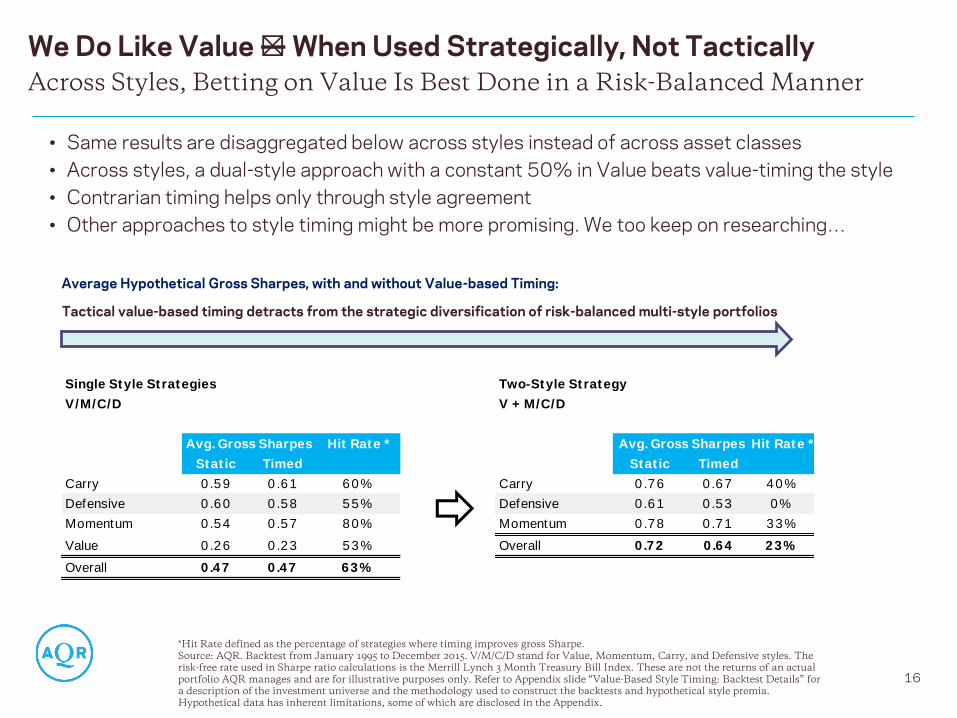
• Same results are disaggregated below across styles instead of across asset classes

• Across styles, a dual-style approach with a constant 50% in Value beats value-timing the style

• Contrarian timing helps only through style agreement

• Other approaches to style timing might be more promising. We too keep on researching…

*Hit Rate defined as the percentage of strategies where timing improves gross Sharpe.

Source: AQR. Backtest from January 1995 to December 2015. V/M/C/D stand for Value, Momentum, Carry, and Defensive styles. The

risk-free rate used in Sharpe ratio calculations is the Merrill Lynch 3 Month Treasury Bill Index. These are not the returns of an actual

portfolio AQR manages and are for illustrative purposes only. Refer to Appendix slide “Value-Based Style Timing: Backtest Details” for

a description of the investment universe and the methodology used to construct the backtests and hypothetical style premia.

Hypothetical data has inherent limitations, some of which are disclosed in the Appendix.

16

Average Hypothetical Gross Sharpes, with and without Value-based Timing:

Tactical value-based timing detracts from the strategic diversification of risk-balanced multi-style portfolios

We Do Like Value •— When Used Strategically, Not Tactically

Across Styles, Betting on Value Is Best Done in a Risk-Balanced Manner

Single Style St rategies Two-Style St rategy

V/M/C/D V + M/C/D

Avg. Gross Sharpes Hit Rate * Avg. Gross Sharpes Hit Rate *

Stat ic Timed Stat ic Timed

Carry 0 .59 0 .61 60% Carry 0 .76 0 .67 40%

Defensive 0 .60 0 .58 55% Defensive 0 .61 0 .53 0%

Momentum 0.54 0 .57 80% Momentum 0.78 0 .71 33%

Value 0 .26 0 .23 53% Overall 0 .72 0 .64 23%

Overall 0 .47 0 .47 63%

17

Source: AQR Whitepaper “Are Defensive Stocks Expensive? A Closer Look at Value Spreads”, Chandra, Ilmanen and Nielsen (2015). Refer to the Appendix for details: -0.9 is the median correlation between changes in value and the returns to 4 asset classes equities, bonds, credits and currencies over the period January 1990 to December 2014. -0.3 is the median correlation between monthly changes in value spreads and/or hypothetical style premia for Value, Momentum, Carry and Defensive over the period January 1990 to December 2014. These are not the returns of an actual portfolio AQR manages and are for illustrative purposes only. Please read important disclosures in the Appendix for a description of the investment universe and the methodology used to construct the backtests. Hypothetical data has inherent limitations some of which are disclosed in the Appendix.

Even Contemporaneous Relations Are Weak Weak Correlation Between Value Spread Changes and L/S Factor Returns

High Correlation in Passive Assets, Weaker for Styles

Co

nte

mp

ora

ne

ou

s R

etu

rn

Change in Value Spreads

Co

nte

mp

ora

ne

ou

s R

etu

rn

Change in Value Spreads

Correlat ion = -0 .9

Intuit ion of a Tight Link... ...but Four Wedges Loosen the Link

Correlat ion = -0 .3

Co

nte

mp

ora

ne

ou

s L

/S R

etu

rn

Typical (Median) Correlation

Long-Only Passive Assets -0.9

Long/Short Factors -0.3

Even before predictions, note the strong contemporaneous correlation between long-only asset valuations and returns, compared to much weaker correlations between L/S style valuations and returns.

Multiple Wedges Loosen the Link

Intuition of a tight link… …but four wedges loosen the link

Wedges Can Even Flip the Sign of the Contemporaneous Relation Example of Defensive Factor Cheapening Coinciding With Outperformance

* BAB here refers to the beta-neutral long/short portfolio that goes long low-beta stocks and short high-beta stocks. The long side is then levered up and the short side is de-levered to achieve beta neutrality. Source: Dividend yield data is from Xpressfeed. Betas are from MSCI Barra’s USE3L model. The universe is a U.S. stock universe that is approximately the top 20th percentile by market-cap and the top 15th percentile by trading volume of U.S. stocks in MSCI Barra’s GEM model universe. Please see AQR Whitepaper “Are Defensive Stocks Expensive? A Closer Look at Value Spreads”, Chandra, Ilmanen and Nielsen (2015) for more information. This is for illustrative purposes only. Hypothetical data has inherent limitations, some of which are disclosed in the Appendix.

- A puzzling example is highlighted in a recent AQR paper “Are Defensive Stocks Expensive? A Closer Look at Style Value Spreads” - U.S. Low Beta style was rich at the end of 2012, Yet U.S. BAB* outperformed in 2013-4 — even as value spreads widened.

18

-7

-6

-5

-4

-3

-2

-1

0

1

2

3

z s

co

re

Low Beta Cheap

Low Beta Expensive

May 2010, Euro Debt Crisis

Aug 2011, US Debt Crisis

Recent widening, 2013 to 2014

1999, Tech bubble

Aug 1998, Russia default

Sep 2008, Financial Crisis

0%

5%

10%

15%

20%

25%

30%

35%

0

0.2

0.4

0.6

0.8

1

1.2

1.4

Cu

mu

lati

ve

Re

turn

to

BA

B

Va

lue

Sp

rea

d

Cumulative Changein Value Spread

Cumulative return toBAB

Value Spread Widening / Low Beta Cheapening

BAB portfolio up

Standardized Composite Value Spread, Hypothetical Low-Minus-High-Beta Portfolio, 1985-2014

Composite Low-Minus-High-Beta Portfolio Value Spread and Returns of the Hypothetical U.S. BAB Portfolio, 2013-2014

AQR Color

Palette

AQR Cyan

Auxiliary Palette

What Might Explain the Surprisingly Uncrowded Factor Theater?

19

Investor Constraints, Funding Sources, Heterogeneous Designs

Source: AQR. For illustrative purposes only.

So many asset managers offering and investors demanding factor investing and smart beta; so

many publications and conferences. Yet, we see so little change in value spreads. Why?

1. Most investors have made only modest explicit allocations to style factors and mainly through

long-only smart beta with low active risk — likely due to their constraints (against leverage, etc.)

2. Inflows into factors may largely reflect deallocations from active managers doing similar things

implicitly and less cost-effectively rather than from index funds — less impact on pricing

3. Heterogeneity in design choices and implementation skill across managers means that all quants

are not doing the same thing (even within one style in one asset class, let alone many)

Crowding Concerns – Final Thoughts

20

Value Spreads May Be the Best But Not the Only Crowding Measures

Besides value spreads, other indicators include excess correlations, short interest, ownership intensity

and other holdings data, etc.

• See, for example, Lou-Polk (2014): “Comomentum”; MSCI (2015): “Lost in the Crowd”; DB

Quantitative Strategy (2016): “Strategy Crowding”

• AUM estimates are not very helpful (wrong units, partial picture…)

Overcrowding can result either in a gradual decay of strategy profits or in sharp losses amid

deleveraging events (cf. quant crisis 2007, LTCM episode 1998, portfolio insurance in 1987)

Trading off overcrowding concerns in well-known factors vs overfitting concerns in novel factors

In conclusion: It makes sense to worry about crowding and monitor it, but we should not overstate the

usefulness of these metrics as tactical trading signals, nor the extremeness of current valuations

• See the debate between Arnott etal. (2016): “How Can ‘Smart Beta’ Go Horribly Wrong?” and

Asness (2016) “The Siren Song of Factor Timing.”

Additional Slides

Why Do We Favor Strategic Over Tactical Allocations?

Tactical style timing/rotation is at least as difficult as market timing. Moreover, the hurdle on timing

skills is higher due to greater “forgone diversification” (next slide).

We believe that strategic diversification across return sources we believe in beats tactical timing.

• Boldly take advantage of that free lunch (if you can stomach the three dirty words…)

• Most investors are arguably strategically underweight the major style premia. Increasing

strategic allocations is the first-order business

• We do not know that risk balance between style premia is optimal but it is an excellent starting

point given our belief in bold diversification

Our research on tactical timing signals suggests they are not a Holy Grail.

• We rarely find a major Sharpe ratio improvement versus stable style allocations, except when we

succumb to overfitting and hindsight biases

• Other timing signals may offer more hope than contrarian/value signals

• We keep researching but do not expect that tactical tilts deserve more than a supporting role in

style investing – partly due to the impact of forgone diversification

22

Tactical Predictions Are Imprecise And The Hurdle is High

Source: AQR. Diversification does not eliminate the risk of experiencing investment losses.

54% 58%

66%

56%

62%

72%

0%

10%

20%

30%

40%

50%

60%

70%

80%

0.5 0.0 -0.5

Bre

ak

ev

en

An

nu

al H

it R

ate

Correlation between Assets

Tilting Switching

23

This May Create a Measurable Performance Hurdle

Source: AQR. The model returns above are provided for illustrative purposes only. The model assumes returns are gross of fees and

transaction costs and assumes asset volatilities of 10% and arithmetic Sharpe ratios of 0.5. Strategic 50/50 is a 50/50 capital-weighted

combination of the two assets. The “tilting” strategy applies tilts with an average of +/-25% (maximum of +/-50%, i.e., asset weights can vary

from 0-100%). The “switching” strategy illustrates the extreme case of tactically switching capital entirely from one asset to the other.

Transaction costs will likely further penalize tactical strategies. The breakeven hit rates are based on breakeven theoretical arithmetic

information ratios, gross of costs and fees, and normally-distributed serially-uncorrelated returns. Hypothetical data has inherent

limitations, some of which are disclosed in the Appendix. Please read important disclosures in the Appendix.

Hypothetical Sharpe Ratios of Model 2-Asset Portfolios Based on random tactical bets

Hypothetical Breakeven Hit Rates for Tactical Tilts Tilts must achieve these hit rates just to regain the expected Sharpe ratio of the strategic portfolio

Not enough to be right “51% of the time”. The hurdle is especially high for portfolios with more

diversified investments, or for more aggressive tilts.

50%

Tactical Investors Forgo Diversification

0.58

0.71

1.00

0.55

0.61

0.71

0.50 0.50 0.50

0.0

0.1

0.2

0.3

0.4

0.5

0.6

0.7

0.8

0.9

1.0

0.5 0.0 -0.5

Ex

pe

cte

d G

ros

s S

ha

rpe

Ra

tio

Correlation between Assets

Strategic 50/50 Tilting Switching

Mean-variance analysis with even heavily discounted historical return inputs may often point to large

portfolio weights for alternative risk premia (compared with long-only asset classes)

Yet, many appealing and diversifying return sources are only modestly used. Why? “The 4Cs”:

• Conviction: investor uncertainty about the sustainability of non-equity premia

• Constraints: aversion to leverage, shorting and derivatives

• Conventionality: “better to fail conventionally” – Keynes

• Capacity: limitations may apply especially for very large investors

The 4Cs also help explain why investors “prefer” equity risk concentration and long-only portfolios,

and why the diversifying style premia are not likely to be “arbed away” soon. Still, it makes sense to

assume lower Sharpe ratios for the future.

24

Source: AQR.

Why Do Many Investors Underutilize Alternative Risk Premia? The 4 Cs Drive Real-World Investor Behaviour

Can Trend Following Cushion Against Financial Calamities?

25

Performed Well in Severe Market Downturns – If Protracted Events

Source: AQR. The Hypothetical Trend-Following Strategy performance is a backtest, net of 2/20 fees and estimated transaction costs.

The 60/40 portfolio has 60% invested in S&P 500 and 40% invested in U.S. 10-year bonds. The portfolio is rebalanced monthly, and no

fees or transaction costs are subtracted from the returns. Please read performance disclosures in the Appendix for a description of the

investment universe and the allocation methodology used to construct the Trend-Following Strategy. Markets considered only where

data existed during the time period. Chart is provided for illustrative purposes only and is not based on an actual portfolio AQR

manages. Hypothetical data has inherent limitations, some of which are disclosed in the Appendix hereto. Past performance is not a

guarantee of future performance.

Panic of

1893

Panic of

1907

WWI

Great

Depression

Recession of 1937-1938

Stagflation

Oil Crisis

1987 Stock

Market Crash

Dot-com

Bubble

Bursting

Global

Financial

Crisis

-80%

-60%

-40%

-20%

0%

20%

40%

60%

80%

100%

120%

Feb 1893 -Aug 1893

Oct 1906 -Dec 1907

Dec 1916 -Dec 1917

Sep 1929 -June 1932

Mar 1937 -Mar 1938

Dec 1968 -Jun 1970

Jan 1973 -Sep 1974

Sep 1987 -Nov 1987

Sep 2000 -Sep 2002

Nov 2007 -Feb 2009

60/40 Portfolio Returns Trend-Following Returns

Hypothetical Performance During the 10 Largest Drawdowns for a 60/40 Portfolio

January 1880 – December 2015

Appendix

27

Antti Ilmanen, Principal, Portfolio Solutions Group

Antti Ilmanen, a Principal at AQR, manages the Portfolio Solutions Group, which advises institutional investors and sovereign wealth funds, and develops AQR’s broad investment ideas. Before AQR, Antti spent seven years as a senior portfolio manager at Brevan Howard, a macro hedge fund, and a decade in a variety of roles at Salomon Brothers/Citigroup. He began his career as a central bank portfolio manager in Finland. Antti earned a Ph.D. in finance from the University of Chicago and M.Sc. degrees in economics and law from the University of Helsinki. Over the years, he has advised many institutional investors, including Norway’s Government Pension Fund Global and the Government of Singapore Investment Corporation. Antti has published extensively in finance and investment journals and has received the Graham and Dodd award and the Bernstein Fabozzi/Jacobs Levy award for his articles. His book Expected Returns (Wiley, 2011) is a broad synthesis of the central issue in investing..

Today’s Presenter

Contemporaneous Correlations

28

This analysis is for illustrative purposes only and is not based on an actual portfolio AQR manages.

1. Source: Returns from Datastream, Bloomberg and Global Financial Database (GFD). U.S. Equities refer to the MSCI US from 1970 to 2014. U.S. Bonds refer to

10-year Treasuries from 1970 to 2014, returns are duration hedged to 7 years. 10-year Expected Inflation from the Survey of Professional Forecasters, Consensus

Economics and the Federal Reserve as described in Ilmanen [2011]. High Yield refers to the Markit High Yield 5-year CDS Index from 2004 and the Barclays

High Yield from 1990 to 2004, as a proxy. For Currencies we take the average correlation across three baskets that are long either of the yen, the euro

(Deutschemark prior to 1999) or sterling and short the U.S. dollar. Purchasing Power Parity from Penn World tables, augmented with OECD data and goes back

to 1970. Real Bond yield is defined as Nominal Bond Yield – Expected Inflation. Default Adjusted Credit Spread is defined as Credit Spread – (1-Recovery

Rate)*(Expected Default Probability Rate), with Recovery Rate assumed to be the rough historical average of 40%. Expected Default Probability Rate is derived

from regression based models that include as inputs index constituent credit spreads and data on bank credit from the Federal Reserve.

2. Source: Please read important disclosures in the Appendix for a description of the investment universe and the methodology used to construct the backtests.

Hypothetical data has inherent limitations some of which are disclosed in the Appendix.

Correlations Between Changes in Value (Spreads) and Returns

Contemporaneous Correlations of Changes in Value Spreads With Returns to Hypothetical U.S. Low-Minus-High-Beta Portfolios2

December 1984–December 2014

Asset Class Value measure

Correlat ion

with Excess

Returns

U.S. Equit ies Book-to-price -0 .90

U.S. Bonds Real Bond Yield -0 .92

U.S. High Yield Default Adjusted Credit Spread -0 .71

Currencies (G4) Purchasing Power Parity -0 .92

Contemporaneous Correlations of Monthly Changes in Value Spreads with Asset Class Returns1

December 1984–December 2014

Dollar Neutral Beta Neutral

Book-to-Price -0.52 -0.18

Operating Cash Flow-to-Enterprise Value -0.44 -0.17

Trailing Earnings-to-Price -0.19 0.05

Forward Earnings-to-Price -0.24 -0.11

Sales-to-Enterprise Value -0.54 -0.22

Average -0.31 -0.13

Contemporaneous Correlations Across Styles

29

Source: AQR. Data for Emerging Equities from 1996 and for Emerging Currencies from 1997. Financial data and prices from

Bloomberg, Datastream, Consensus Economics, Xpressfeed, MSCI Barra and Penn World tables. All data is monthly. Styles are returns

to hypothetical portfolios as defined in Ilmanen, Israel and Moskowitz (2012), This analysis is for illustrative purposes only and is not

based on an actual portfolio AQR manages. Hypothetical data has inherent limitations some of which are disclosed in the Appendix.

Contemporaneous Correlations of Changes in Value Spreads with Returns to Hypothetical Multi-Asset L/S Style Portfolios January 1990 –December 2014

Asset Class / Market Value Momentum Carry Defensive

Macro Commodit ies -0 .70 -0 .36 -0 .35

Developed Equit ies -0 .34 -0 .13 -0 .17

Emerging Equit ies -0 .04 -0 .07 -0 .22

Government Bonds (Developed) -0 .58 -0 .25 -0 .47 -0 .51

Developed Currencies -0 .66 -0 .42 -0 .73

Emerging Currenices -0 .68 -0 .43 -0 .58

Interest Rate Futures (Developed) -0 .56 -0 .34 -0 .21

Industry Japan Industry Select ion -0 .22 -0 .18 -0 .36

Select ion Europe ex. U.K. Industry Select ion -0 .29 -0 .28 -0 .25

U.K. Industry Select ion -0 .18 -0 .17 -0 .29

U.S. Industry Select ion -0 .14 -0 .18 -0 .27

Stock Japan Stock Select ion -0 .26 -0 .28 -0 .20

Select ion Europe ex. U.K. Stock Select ion -0 .40 -0 .20 -0 .05

U.K. Stock Select ion -0 .42 -0 .23 -0 .18

U.S. Stock Select ion -0 .25 -0 .32 -0 .22

Average -0 .38 -0 .26 -0 .47 -0 .25

Construction of Trend-Following Backtest

Trend-Following Strategy The Trend-Following Strategy was constructed with an equal-weighted combination of 1-month, 3-month, and 12-month Trend-Following strategies for 67 markets across 4 major asset classes –29 commodities, 11 equity indices, 15 bond markets, and 12 currency pairs – from January 1880 to June 2015. Since not all markets have return data going back to 1880, we construct the strategies using the largest number of assets for which return data exist at each point in time. We use futures returns when they are available. Prior to the availability of futures data, we rely on cash index returns financed at local short rates for each country. In order to calculate net-of-fee returns for the time series momentum strategy, we subtracted a 2% annual management fee and a 20% performance fee from the gross-of-fee returns to the strategy. The performance fee is calculated and accrued on a monthly basis, but is subject to an annual high-water mark. In other words, a performance fee is subtracted from the gross returns in a given year only if the returns in the fund are large enough that the fund’s NAV at the end of the year exceeds every previous end of year NAV. The transactions costs used in the strategy are based on AQR’s 2012 estimates of average transaction costs for each of the four asset classes, including market impact and commissions. The transaction costs are assumed to be twice as high from 1993 to 2002 and six times as high from 1880–1992, based on Jones (2002). The transaction costs used are as follows: The 2014 estimate of assets under management in the BarclayHedge Systematic Traders index is $280 billion. We looked at the average monthly holdings in each asset class (calculated by summing up the absolute values of holdings in each market within an asset class) for our time series momentum strategy since 2000, run at a NAV of $280 billion, and compared them to the size of the underlying cash or derivative markets. For equities, we use the total global equity market capitalization estimate from the October 2014 World Federation of Exchanges (WFE) monthly statistics tables. For bonds, we add up the total government debt for the 15 developed countries with the largest debt using Bloomberg data. For currencies, we use the total notional outstanding amount of foreign exchange derivatives, excluding options, which are U.S. dollar denominated in the first half of 2014 from the Bank for International Settlements (BIS) November 2014 report. For commodities, we use the total notional of outstanding OTC commodities derivatives, excluding options, in the first half of 2014 from the BIS November 2014 report and add the aggregate exchange futures open interest for 31 of the most liquid commodities.

30

Methodology:

• Rebalance Frequency: Monthly

• Signal: Expanding window DIFF 1 value spread z-score with minimum 60 months history, capped at +/- 2 STD

• Period: 1995 to Dec 2015 2 (starts in 1995 to allow 60m of value spreads for the expanding z-scores)

• Style Returns: Ex-ante constant vol style returns, gross of t-costs

• Weighting: Styles are scaled proportionate to the value spread z-scores, in a range of 50% to 150% of the static model weight on

the style. No shorting of styles.

• For single-style strategies, we vary the ex-ante risk of the style based on it’s value spread z-score.

• Scaling factor = (z-score + 4) / 4 3

• Weight = Min weight + Scaling factor* (150% - 50%)

• For multi-style strategies, weights for each style are pro-rated up or down so that the weights add up to 100% at each point

in time

• We use a 12m moving average of the value spread z-score as value works at longer horizons.

Caveats:

• Correlations are not used in the backtests to scale weights. So, at the same point in time, the value-timed portfolio could have a different ex-ante vol than the static portfolio.

• For simplicity, the static capital weights assumed are equal-weighted across styles, thus making the styles not equal risk-weighted (since Val and Mom offset each other more). However, the tactical-weights are anchored to these equal capital weights too.

• Even in the timing strategy, as weights are pro-rated to add up to 100% at each point in time 4, if all styles are cheap at the same, then the strategy will still underweight the style that is less cheap than the others.

1. Results available for RATIO value spreads, but these cannot be used for Macro styles

2. Backtest upto Sep 2015 for UK and ROE Stock Selection styles

3. Because the range of possible z-scores is 4 STD from -2 STD to +2 STD

4. That is, irrespective of the agreement/correlation across factors, the backtest takes 100% weight (to mimic constant vol)

Source: AQR. Please read important disclosures in the Appendix for a description of the investment universe and the methodology used to construct

the backtests and hypothetical style premia. Hypothetical data has inherent limitations some of which are disclosed in the Appendix.

31

Value Timing Backtest Methodology Under/Over-weight Styles Based on 12m Moving Average Value Spreads STD

Macro Environmental Indicators / Investment Returns

32

Macro Indicators We choose to construct macro indicators, or risk factors, mainly based on fundamental economic data, and not based on asset market returns (which are “too close” to the patterns we try to explain). For example, potential market–based proxies of economic growth include equity market returns, the relative performance of cyclical industries, dividend swaps, and estimates from cross–sectional regressions of asset returns on growth surprises. This choice brings its own problems, notably timing challenges as macroeconomic data are backward-–looking, published with lags and later revised, while asset prices are clearly forward–looking. The impact of publication lags and the mismatch between backward– and forward–looking perspectives can be mitigated by using longer windows. Thus, we use contemporaneous annual economic data and asset returns through our analysis (past–year data with quarterly overlapping observations). Arguably composite growth surprise indices are the best proxies of economic growth news, but such composites are available at best going back to 1990s. Forecast changes in economist surveys as well as business and consumer confidence surveys may be the next best choices because they are reasonably forward-looking and timely. In a globalized world, it is not clear whether we should focus only on domestic macro developments, but data constraints make us focus on U.S. data. Finally, it is not clear how real economic growth ties to expected corporate cash flow growth (e.g., earnings per share) that influence stock prices or to real yields that influence all asset prices but especially those of bonds. Each of our macro indicators combines two series, which are first normalized to Z–scores: that is, we subtract a historical mean from each observation and divide by a historical volatility. When we classify our quarterly 12–month periods into, say, ‘growth up’ and ‘growth down’ periods, we compare actual observations to the median so as to have an equal number of up and down observations (because we are not trying to create an investable strategy where data should be available for investors in real time, we use the full sample median). The underlying series for our growth indicator are the Chicago Fed National Activity Index (CFNAI) and the “surprise” in industrial production growth over the past year. Since there is no uniquely correct proxy way to capture “growth”; averaging may make the results more robust and signals appropriate humility. CFNAI takes this averaging idea to extremes as it combines 85 monthly indicators of U.S. economic activity. The other series – the difference between actual annual growth in industrial production and the consensus economist forecast a year earlier – is narrower but more directly captures the surprise effect in economic developments. We use median forecasts from the Survey of Professional Forecasters data as published by the Philadelphia Fed. While data surprises a priori have a zero mean, this series has exhibited a downward trend in recent decades, reflecting the (partly unexpected) relative decline of the U.S. manufacturing sector. Our inflation indicator is also an average of two normalized series. One series measures the de–trended level of inflation (CPIYOY minus its mean, divided by volatility), while the other measures the surprise element in realized inflation (CPIYOY minus consensus economist forecast a year earlier). Investment Return Series The investment return series we study include both asset class premia and style premia. The former are long-only returns but expressed in excess returns over the Treasury bill rate. The latter are long-short returns and scaled to target or realize 10% annual volatility. We subtract no trading costs or fees, which makes a bigger difference for the long-short strategies. The asset class premia are global equities (MSCI World), global bonds (GDP-weighted average of 10-year government bonds in six countries), and an equal-weighted composite of 24 commodity futures. The market-neutral style premia (Value, Momentum, Carry and Defensive) are hypothetical long/short strategies applied in multiple asset classes: stock selection, industry allocation, country allocation in equity, fixed income and currency markets, and commodities. Each style premia strategy allocates 50/50 risk weights to stock and industry selection (SS) and asset allocation (AA) strategies. For SS we use 50/50 risk weights between stock selection within industries and across industries (to be in line with the common but arguably inefficient practice of letting across-industry positions matter as much as within-industry positions). For AA we use the same relative risk weights for asset classes as “Investing With Style” (AQR white paper, 2012, available upon request): 33% equity country allocation, 25% fixed income, 25% currencies, 17% commodities. We combine several data sources to produce a dataset long enough to capture many different macroeconomic environments: • Since 1990, we use value, momentum, carry and defensive style premia strategies as described in “Investing With Style” (AQR white paper, 2012, available upon request), except for SS carry, for which we use the dividend yield strategy returns in Ken French’s data library. • For 1972-1989, we source value and momentum style returns from “Value and Momentum Everywhere” (Journal of Finance, 2013), defensive style returns from “Betting Against Beta” (Journal of Financial Economics, 2013), and SS carry from the dividend yield strategy returns in Ken French’s data library. We construct the AA carry style premia before 1990 as well as some early histories of AA value, momentum and defensive styles using AQR in-house backtests. These backtests are similar to those described above, but over a narrower universe. While the SS style premia proxies we use since 1990 are market (beta) neutral, the value and momentum premia before 1990, and the carry premium throughout, are ‘only’ dollar-neutral and may contain moderate empirical beta exposures. The defensive style premia are beta-neutral through the whole sample (we buy larger amounts of low-risk investments than we sell high-risk investments), which means that they are actually not as defensive as the dollar-neutral quality style. (The general lesson is that we need to be precise in understanding strategy designs. Just as corporate bond positions will have very different market exposures depending on whether they are duration-hedged with Treasuries, market exposures of style premia will depend on the degree of hedging). The Trend series used here is the Moskowitz, Ooi, and Pedersen (2012) specification that assesses trends based on past 12-month returns on 9 equity indices, 13 developed bond markets, 10 currency exchange rates, and 24 commodity futures. Please see “Time Series Momentum” (Moskowitz, Ooi, and Pedersen, 2012) for more information on the construction of this series.

Construction of Long/Short Style Premia

AQR backtests of Value, Momentum, Carry and Defensive theoretical long/short style components are based on monthly returns, undiscounted, gross of fees and transaction costs, excess of a cash rate

proxied by the Merrill Lynch 3-Month T-Bill Index, and scaled to 12% annualized volatility. Each strategy is designed to take long positions in the assets with the strongest style attributes and short

positions in the assets with the weakest style attributes, while seeking to ensure the portfolio is market-neutral. The Style Premia Strategy portfolio is based on the target asset group allocations included

herein, roughly equally risk weighting styles within the asset group, resulting in a style allocation of approximately 34% to Value, 34% to Momentum, 18% to Defensive and 14% to Carry. The AQR

backtest of the Style Premia Strategy is based on monthly returns, excess of a cash rate proxied by the Merrill Lynch 3-Month T-Bill Index and heavily discounted to reflect uncertainty in historical costs

and opportunities; targeting 12% annualized volatility. The Style and Asset Group Composites, are based on an allocation to the style components and asset group components based on their liquidity

and breadth. The components are then allocated with roughly equal weighting to each of the styles within an asset group (as not all four styles are present in each asset group). Please see below for a

description of the Universe selection.

Stock and Industry Selection: approximately 2,000 stocks across Europe, Japan, and U.S. Country Equity Indices: Developed Markets: Australia, Canada, Eurozone, Hong Kong, Japan, Sweden,

Switzerland, U.K., U.S. Within Europe: Italy, France, Germany, Netherlands, Spain. Emerging Markets: Brazil, China, India, Israel, Malaysia, Mexico, Poland, Singapore, South Africa, South Korea, Taiwan,

Thailand, Turkey. Bond Futures: Australia, Canada, Germany, Japan, U.K., U.S. Yield Curve: Australia Germany, United States. Interest Rate Futures: Australia, Canada, Europe (Euribor), U.K. and U.S.

(Eurodollar). Currencies: Developed Markets: Australia, Canada, Euro, Japan, New Zealand, Norway, Sweden, Switzerland, U.K., U.S. Emerging Markets: Brazil, Hungary, India, Israel, Mexico, Poland,

Singapore, South Africa, South Korea, Taiwan, Turkey. Commodity Selection: Silver, copper, gold, crude, Brent oil, natural gas, corn, soybeans.

33

Performance Disclosures

34

This presentation cannot be used in a general solicitation or general advertising to offer or sell interest in its Funds. As such, this information cannot be included in any

advertisement, article, notice or other communication published in any newspaper, magazine, or similar media or broadcast over television or radio; and cannot be used

in any seminar or meeting whose attendees have been invited by any general solicitation or general advertising.

Firm Information:

AQR is a Connecticut based investment advisor registered with the Securities and Exchange Commission under the Investment Advisors Act of 1940. AQR conducts trading and

investment activities, specializing in global asset allocation and global stock selection involving a broad range of instruments, including, but not limited to, individual equity and

debt securities, currencies, futures, commodities, fixed income products and other derivative securities.

For purposes of Firm wide compliance and Firm wide total assets, AQR defines the “Firm” as entities controlled by or under common control with AQR (including voting power).

The Firm is comprised of AQR, CNH Partners, LLC (“CNH”), AQR Re Ltd. (AQR Re) and AQR Funds.

Upon request AQR will make available a complete list and description of all of Firm composites, as well as additional information regarding the policies for valuing portfolios,

calculating performance, and preparing compliant presentations.

Past performance is not an indication of future performance.

Fees: Returns are calculated net of all withholding taxes on foreign dividends. Accruals for fixed income and equity securities are included in calculations. Gross of fees returns

are calculated net of transaction costs and gross of operating expenses. Operating expenses may include, but are not limited to Management, Custodial, Administrative, and legal

fees. Additional information regarding fees and the calculation of Gross and Net performance is available upon request. AQR’s management or advisory fees are described in Part

2A of its Form ADV. In addition, AQR funds may have a redemption charge of 2% based on gross redemption proceeds that may be charged upon early withdrawals. Consultants

supplied with gross results are to use this data in accordance with SEC, CFTC and NFA guidelines.

AQR’s asset based fees for portfolios within the composite may range up to 1.50% of assets under management, and are generally billed monthly or quarterly at the

commencement of the calendar month or quarter during which AQR will perform the services to which the fees relate.

AQR Capital Management, LLC Style Premia Composite 8/31/12–12/31/14

* Merrill Lynch 3-Month Treasury Bill Index

Year Gross return

%

Net Return

%

Benchmark*

Return %

Number of

Portfolios

Composite

Assets ($ M)

Total Firm

Assets ($ M)

2012 -1.20 -1.69 0.05 1 6.76 71,122.42

2013 29.84 27.95 0.07 1 1,041.75 98,302.69

2014 13.36 11.69 0.03 1 3,038.15 122,655.99

Performance Disclosures

Composite Characteristics: The Style Premia Composite (The Composite) was created September 1st, 2012. The Composite's strategy seeks to deliver efficient exposure to a well-diversified portfolio of

long-short style strategies across six asset group contexts including Stock and Industry Selection, Equity Indices, Bonds, Interest Rates, Currencies, and Commodities. AQR pursues these goals by

investing in instruments not limited to Stocks, Futures, Swaps, and Currency Forwards. The Composite's strategy targets the highest ex ante volatility relative to all of the Firm's Style Premia Composites.

The Composite is denominated in USD. The composite benchmark is the Merrill Lynch 3 Month Treasury Bill Index. The index measures the rate of return an investor would realize when purchasing a

single US 3 month treasury bill, holding it for one month, selling it, and rolling it into a newly selected issue at the beginning of the next month. The investments in the Composite vary substantially from

those in the Benchmark. The index has not been selected to represent an appropriate benchmark to compare an investor’s performance, but rather is disclosed to allow for comparison of the investor’s

performance to that of a certain well-known and widely recognized index. Where applicable, the Master account is considered in lieu of its full volatility feeders because said feeders are one hundred

percent invested in the Master Account.

Composite Net of fee performance results are calculated by deducting from the gross Composite monthly return the maximum management or advisory fee charged by AQR to a new portfolio in the

composite. The standard model management fee per annum for this Composite is 1.50%. Composite assets may have been exposed to the impact of performance fees.

Composites will exclude terminated portfolios after the last full calendar month performance measurement period that the assets were under management. The Composite will continue to include the

performance results for all periods prior to termination. New accounts that fit the composite definition are added at the start of the first full calendar month after the assets come under management, or

after it is deemed that the investment decisions made by the investment advisor fully reflect the intended investment strategy of the portfolio.

In March of 2015 AQR removed its significant cash flow policy. Additional information on this decision is available upon request.

Calculation Methodology: Individual portfolios are revalued monthly or intra-month when cash flows occur. Gross of fees returns are calculated gross of management, administrative and custodial fees

and net of transaction costs. Composite returns are asset-weighted based on the constituents’ month beginning asset value. The firm links returns geometrically to produce an accurate time-weighted

rate of return. The dispersion measure is the equal-weighted standard deviation of accounts in the composite for the entire year. Dispersion is not considered meaningful for periods shorter than one year

or for periods during which the composite contains five or fewer accounts for the full period. The three-year annualized ex-post standard deviation measure is inapplicable when 36 monthly returns are not

available.

Other Disclosures: AQR claims compliance with the Global Investment Performance Standards (GIPS) and has prepared and presented this report in compliance with the GIPS standards. AQR has been

independently verified for the period August 1998 through December 2014. Verification assesses whether (1) the firm has complied with all the composite construction requirements of the GIPS

standards on a firm-wide basis and (2) the firm’s policies and procedures are designed to calculate and present performance in compliance with the GIPS standards. The Style Premia Composite has been

examined for the periods from its inception through December 31, 2014. The Verification and performance examination reports are available upon request.

Benchmark returns are not covered by the report of independent verifiers.

AQR may engage in leveraged, derivative, and short positions in order to meet its performance objectives. The use of these positions may have a material impact on performance results. Additionally,

there may be subjective unobservable inputs used in the valuation of certain financial instruments utilized by certain AQR managed investment vehicles. The risks inherent to the strategies employed by

accounts included are set forth in the applicable offering documents and other information provided to potential subscribers, from where more detailed information regarding the extent to which leverage,

derivatives, and short positions can be obtained. These are available on request, if not provided along with this presentation itself.

35

36

This document has been provided to you solely for information purposes and does not constitute an offer or solicitation of an offer or any advice or recommendation to purchase any securities or other

financial instruments and may not be construed as such. The factual information set forth herein has been obtained or derived from sources believed to be reliable but it is not necessarily all-inclusive and

is not guaranteed as to its accuracy and is not to be regarded as a representation or warranty, express or implied, as to the information’s accuracy or completeness, nor should the attached information

serve as the basis of any investment decision. This document is intended exclusively for the use of the person to whom it has been delivered and it is not to be reproduced or redistributed to any other

person.

There is no guarantee, express or implied, that long-term return and/or volatility targets will be achieved. Realized returns and/or volatility may come in higher or lower than expected. PAST

PERFORMANCE IS NOT A GUARANTEE OF FUTURE PERFORMANCE. Diversification does not eliminate the risk of experiencing investment losses.

Hypothetical performance results (e.g., quantitative backtests) have many inherent limitations, some of which, but not all, are described herein. No representation is being made that any fund or account

will or is likely to achieve profits or losses similar to those shown herein. In fact, there are frequently sharp differences between hypothetical performance results and the actual results subsequently

realized by any particular trading program. One of the limitations of hypothetical performance results is that they are generally prepared with the benefit of hindsight. In addition, hypothetical trading does

not involve financial risk, and no hypothetical trading record can completely account for the impact of financial risk in actual trading. For example, the ability to withstand losses or adhere to a particular

trading program in spite of trading losses are material points which can adversely affect actual trading results. The hypothetical performance results contained herein represent the application of the

quantitative models as currently in effect on the date first written above and there can be no assurance that the models will remain the same in the future or that an application of the current models in the

future will produce similar results because the relevant market and economic conditions that prevailed during the hypothetical performance period will not necessarily recur. There are numerous other

factors related to the markets in general or to the implementation of any specific trading program which cannot be fully accounted for in the preparation of hypothetical performance results, all of which

can adversely affect actual trading results. Discounting factors may be applied to reduce suspected anomalies. This backtest’s return, for this period, may vary depending on the date it is run.

Hypothetical performance results are presented for illustrative purposes only. In addition, our transaction cost assumptions utilized in backtests , where noted, are based on AQR's historical realized

transaction costs and market data. Certain of the assumptions have been made for modeling purposes and are unlikely to be realized. No representation or warranty is made as to the reasonableness of

the assumptions made or that all assumptions used in achieving the returns have been stated or fully considered. Changes in the assumptions may have a material impact on the hypothetical returns

presented. Hypothetical performance is gross of advisory fees, net of transaction costs, and includes the reinvestment of dividends. If the expenses were reflected, the performance shown would be

lower. Where noted, the hypothetical net performance data presented reflects the deduction of a model advisory fee and does not account for administrative expenses a fund or managed account may

incur. Actual advisory fees for products offering this strategy may vary.

Gross performance results do not reflect the deduction of investment advisory fees, which would reduce an investor’s actual return. For example, assume that $1 million is invested in an account with the

Firm, and this account achieves a 10% compounded annualized return, gross of fees, for five years. At the end of five years that account would grow to $1,610,510 before the deduction of management

fees. Assuming management fees of 1.00% per year are deducted monthly from the account, the value of the account at the end of five years would be $1,532,886 and the annualized rate of return

would be 8.92%. For a ten-year period, the ending dollar values before and after fees would be $2,593,742 and $2,349,739, respectively. AQR’s asset based fees may range up to 2.85% of assets

under management, and are generally billed monthly or quarterly at the commencement of the calendar month or quarter during which AQR will perform the services to which the fees relate. Where

applicable, performance fees are generally equal to 20% of net realized and unrealized profits each year, after restoration of any losses carried forward from prior years. In addition, AQR funds incur

expenses (including start-up, legal, accounting, audit, administrative and regulatory expenses) and may have redemption or withdrawal charges up to 2% based on gross redemption or withdrawal

proceeds. Please refer to AQR’s ADV Part 2A for more information on fees. Consultants supplied with gross results are to use this data in accordance with SEC, CFTC, NFA or the applicable jurisdiction’s

guidelines.

Performance Disclosures