STURM SEQUENCES AND RANDOM EIGENVALUE DISTRIBUTIONS

JAMES T. ALBRECHT, CY P. CHAN, AND ALAN EDELMAN

Abstract. This paper proposes that the study of Sturm sequences is invaluable in the nu-merical computation and theoretical derivation of eigenvalue distributions of random matrixensembles. We first explore the use of Sturm sequences to efficiently compute histogramsof eigenvalues for symmetric tridiagonal matrices and apply these ideas to random matrixensembles such as the β-Hermite ensemble. Using our techniques, we reduce the time tocompute a histogram of the eigenvalues of such a matrix from O(n2 + m) to O(mn) timewhere n is the dimension of the matrix and m is the number of bins (with arbitrary bincenters and widths) desired in the histogram (m is usually much smaller than n). Second,we derive analytic formulas in terms of iterated multivariate integrals for the eigenvaluedistribution and the largest eigenvalue distribution for arbitrary symmetric tridiagonal ran-dom matrix models. As an example of the utility of this approach, we give a derivation ofboth distributions for the β-Hermite random matrix ensemble (for general β). Third, weexplore the relationship between the Sturm sequence of a random matrix and its shootingeigenvectors. We show using Sturm sequences that, assuming the eigenvector contains nozeros, the number of sign changes in a shooting eigenvector of parameter λ is equal to thenumber of eigenvalues greater than λ. Finally, we use the techniques presented in the firstsection to experimentally demonstrate a O(log n) growth relationship between the varianceof histogram bin values and the order of the β-Hermite matrix ensemble.

This paper is dedicated to the fond memory of James T. Albrecht

1. Introduction

A computational trick can also be a theoretical trick. The two go together probably moreoften than noticed. Perhaps the constraints of machines come from the same “fabric” thatis woven into mathematics itself.

In this case we noticed a cute trick: we can histogram without histogramming. Math-ematically, we get new formulas for level densities and largest eigenvalue distributions interms of iterated integrals. Many numerical experiments in random matrix theory computethe eigenvalues of random matrices and then histogram. What else would one do other thaneig of as many matrices as possible (perhaps computed from randn), followed by hist? Theanswer is that mathematics is kind, and one can compute histogram information without thenumerical computation of eigenvalues. One remembers that the Sturm sequence computesthe number of eigenvalues less than any “cut” (see Section 2 for elaboration). This paperproposes that this is not only a cute computational trick for efficiency, but a very importanttheoretical tool in the study of random matrix theory.

2000 Mathematics Subject Classification. Primary 15A52, 15A18 ; Secondary 15A90.Key words and phrases. Sturm sequences, Random matrices, β-Hermite ensemble, Eigenvalue histogram-

ming, Largest eigenvalue distribution, Level densities, Shooting Eigenvectors, Histogram variance.Communicated by Andrew Odlyzko.This research was supported by NSF Grant DMS–0411962.

1

We begin the paper by exploring the use of Sturm sequences as a computational toolto efficiently compute histograms of eigenvalues for symmetric tridiagonal matrices. Sturmsequences are currently available in LAPACK when computing eigenvalues of symmetrictridiagonal matrices (via the DLAEBZ routine, which is called by the DSTEBZ routine).Other alternatives for the symmetric tridiagonal problem can also be found with routinesstarting with the prefix DST, though none explicitly compute a histogram of eigenvalues.

As mentioned in [4], a substantial computational savings to histogramming can be achievedvia Sturm sequence methods. Since tridiagonal matrix models exist for certain classical ran-dom matrix ensembles [3], the techniques presented here can be applied to these ensembles.Using this method, we can compute a histogram of the eigenvalues of such a matrix in O(mn)time where n is the dimension of the matrix and m is the number of bins (with arbitrary bincenters and widths) desired in the histogram. Using the naive approach of computing theeigenvalues and then histogramming them, computing the histogram would cost O(n2 +m)time. Our algorithm is a significant improvement because m is usually much smaller thann. For example, we reduced the time to compute a 100 bin histogram of the eigenvaluesof a 2000 × 2000 matrix from 470 ms to 4.2 ms. This algorithm allows us to compute his-tograms that were computationally infeasible before, such as those for n equal to 1 billion.(As an aside, for those interested in the question of computing the largest eigenvalue of theβ-Hermite ensemble quickly, we refer to one of the author’s talks [6].)

In the second part of this paper, we describe a theoretical use of Sturm sequences, givingboth the eigenvalue distribution (also called the level density) and the largest eigenvalue dis-tribution of β-Hermite random matrix ensembles for arbitrary values of β. When normalizedproperly, the eigenvalue distribution converges to the well known Wigner semicircle [15], andthe largest eigenvalue distribution to the Tracy-Widom distribution [13]. We derive analyticformulas in terms of multivariate integrals for any n and any β by analyzing the Sturmsequence of the tridiagonal matrix model. The formulas provided here are quite general andcan also be generalized beyond the Hermite distribution.

Our main theoretical results are as follows. We show in Section 4.1 that the eigenvaluedistribution of a matrix can be expressed as

Pr[Λ < λ] =1

n

n∑i=1

Pr[ri,λ < 0] =1

n

n∑i=1

∫ 0

−∞fri

(s) ds, (see Theorem 4.1)

where ri,λ is the ith element of the Sturm ratio sequence (r1,λ, r2,λ, . . . , rn,λ). When appliedto the β-Hermite random matrix ensemble in Section 5.1, the marginal densities fri

(s) arederived by iterated multiplication and integration of the conditional density

fri|ri−1(si|si−1) =

|si−1|pi

√2π

e−14[2(si+λ)2−z2

i ]D−pi(zi), (see Corollary 5.3)

where D is the parabolic cylinder function, pi = 12β(i− 1), and zi = sign(si−1)(si +λ+ si−1).

In Section 4.2, we show that the largest eigenvalue distribution of a matrix can be describedin terms of the joint density fr1,r2,...,rn of the Sturm ratio sequence:

Pr[Λmax < λ] =

∫ 0

−∞

∫ 0

−∞· · ·

∫ 0

−∞fr1,r2,...,rn(s1, s2, . . . , sn) ds1ds2 . . . dsn. (see Theorem 4.2)

For the β-Hermite ensemble, the joint density fr1,r2,...,rn can be derived from the conditionaldensity by iterated multiplication as above.

2

As a guide to the reader, the table below shows where the formal results may be found:

General Case Hermite Case (GOE, GUE, GSE, . . . )

Level Density Theorem 4.1Corollary 5.3

(Corollary 5.7 contains an alternate formulation)Largest Eigenvalue Theorem 4.2 Corollary 5.4

This work generalizes a number of formulas, some very well known. The Hermite leveldensity formula for β = 2 (and under the appropriate normalization) is

fn(x) =n−1∑k=0

Cke−x2

Hk(x)2

for constants Ck and Hermite polynomials Hk(x) (see Mehta [10, eq. (6.2.10)]). Mehta alsocovers the β = 1 [10, eq. (7.2.32)] and β = 4 [10, second paragraph of page 178] cases.An iterated contour integral formula appears in Forrester and Desrosiers [2]. For even β,Forrester and Baker [1] present a formula using a Hermite polynomial of a matrix argument.In Dumitriu, Edelman, and Shuman [5, page 39], this density appears in the form (usingα ≡ 2/β):

fn(x) =1√2π

(−1)n/α Γ(1 + 1α)

Γ(1 + nα)e−x2/2Hα

[(2/α)n−1](xIn).

Software is also provided in [5], and examples are given for the evaluation. Results forLaguerre and other densities are also known in some cases, including those found in theabove cited references. There are differential equations that describe the largest eigenvaluestatistic for finite n and β = 1, 2, 4 given in [13].

In the third section of this paper, we explore the relationship between the Sturm sequenceof a tridiagonal random matrix A and its shooting eigenvectors. Shooting eigenvectors arethose that result from fixing one value (say x1) of a vector x = (x1, x2, . . . , xn) and solvingfor the rest of its values under the equation (A−λI)x = 0. We show using Sturm sequencesthat, assuming the eigenvector contains no zeros, the number of sign changes in the shoot-ing eigenvector is equal the number of eigenvalues of A greater than λ. This connectionwas inspired by work by Jose Ramirez, Brian Rider, and Balint Virag [11], who proved ananalogous result for stochastic differential operators.

In the final part of this paper, we use the histogramming technique presented in the firstsection to examine the variance of histogram bin values for eigenvalues of the β-Hermiterandom matrix ensemble. By leveraging our new algorithm, we were able to compute thesample variance for each of 100 histogram bins over 1024 trials for n = 1 up to 220 forvarious values of β. We constructed plots of the mean variance as n increases to illustratean O(log n) growth relationship.

As a general comment, some methods described in this paper may refer to symmetrictridiagonal matrices, but they can also be applied to nonsymmetric tridiagonal matricesvia a diagonal similarity transform. Indeed, only the pairwise product of the super- andsub-diagonals, in addition to the diagonal itself, matters.

In Section 2, we review the definition of the Sturm sequence of a matrix and describe someof its properties. In Section 3, we describe an efficient algorithm for computing the histogramof eigenvalues of a symmetric tridiagonal matrix and give empirical performance results. In

3

Section 4, we describe how to derive both the eigenvalue distribution (level density) andthe largest eigenvalue distribution in terms of Sturm ratio sequence elements for arbitrarysymmetric tridiagonal matrices. Section 5 shows how to apply the results from Section 4to derive the densities for the β-Hermite random matrix ensemble. Section 6 describes theconnection between the sign changes in Sturm sequences and those in shooting eigenvectors,and Section 7 examines the mean variance of histogram bins for the β-Hermite ensemble.

2. Sturm Sequences

2.1. Definition. Define (A0, A1, A2, . . . , An) to be the sequence of submatrices of an n× nmatrix A anchored in the lower right corner of A. The Sturm sequence (d0, d1, d2, . . . , dn)A

is defined to be the sequence of determinants (|A0|, |A1|, |A2|, . . . , |An|). In other words, di

is the determinant of the i× i lower-right submatrix of A. We define d0, the determinant ofthe empty matrix, to be 1.

A = An =

a11 a12 . . . a1n

a21 a22 . . . a2n...

.... . .

...an1 an2 . . . ann

,

A1 = [ann], A2 =

[an−1,n−1 an−1,n

an,n−1 an,n

], A3 =

an−2,n−2 an−2,n−1 an−2,n

an−1,n−2 an−1,n−1 an−1,n

an,n−2 an,n−1 an,n

, etc.

2.2. Properties.

2.2.1. Counting Negative Eigenvalues. The eigenvalues of principal submatrices of A inter-lace, yielding the following lemma:

Lemma 2.1. The number of sign changes in the Sturm sequence (d0, d1, d2, . . . , dn)A is equalto the number of negative eigenvalues of A.

Proof. See [14, page 228] or [16, pages 103–104]. �

Some extra care has to be taken if zeros are present in the Sturm sequence. In somecases when a short sequence of zeros appears, it can be determined how to assign signs tothe zeros such that Lemma 2.1 still holds. However, if enough zeros occur consecutively,the exact number of negative eigenvalues becomes impossible to determine from the Sturmsequence alone. Fortunately, we do not have to worry about zeros in the Sturm sequence forthe purposes of this paper because, in the case of the β-Hermite ensemble as well most otherrandom matrix ensembles of interest, the probability of any zeros occurring in the Sturmsequence is zero. Therefore, in the interest of simplicity we assume for the remainder of thispaper that no zeros occur in the Sturm sequence.

2.2.2. Sturm Ratio Sequence. Since we are mainly interested in the relative sign of consecu-tive values in the Sturm sequence, we define the Sturm ratio sequence (r1, r2, . . . , rn)A to bethe sequence of ratios of consecutive values in the original Sturm sequence. In other words,

(1) ri = di/di−1 ∀ i ∈ {1, 2, . . . , n}.Lemma 2.2. The number of negative values in (r1, r2, . . . , rn)A equals the number of negativeeigenvalues of A.

4

Proof. From our definition of the Sturm ratio sequence, the number of negative values in thesequence equals the number of sign changes in (d0, d1, d2, . . . , dn)A. From Lemma 2.1, thisin turn is equal to the number of negative eigenvalues of A. �

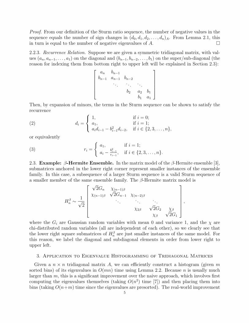
2.2.3. Recurrence Relation. Suppose we are given a symmetric tridiagonal matrix, with val-ues (an, an−1, . . . , a1) on the diagonal and (bn−1, bn−2, . . . , b1) on the super/sub-diagonal (thereason for indexing them from bottom right to upper left will be explained in Section 2.3):

an bn−1

bn−1 an−1 bn−2

. . . . . . . . .b2 a2 b1

b1 a1

Then, by expansion of minors, the terms in the Sturm sequence can be shown to satisfy therecurrence

(2) di =

1, if i = 0;a1, if i = 1;aidi−1 − b2i−1di−2, if i ∈ {2, 3, . . . , n},

or equivalently

(3) ri =

{a1, if i = 1;

ai −b2i−1

ri−1, if i ∈ {2, 3, . . . , n}.

2.3. Example: β-Hermite Ensemble. In the matrix model of the β-Hermite ensemble [3],submatrices anchored in the lower right corner represent smaller instances of the ensemblefamily. In this case, a subsequence of a larger Sturm sequence is a valid Sturm sequence ofa smaller member of the same ensemble family. The β-Hermite matrix model is

Hβn ∼

1√2

√2Gn χ(n−1)β

χ(n−1)β

√2Gn−1 χ(n−2)β

. . . . . . . . .

χ2β

√2G2 χβ

χβ

√2G1

,where the Gi are Gaussian random variables with mean 0 and variance 1, and the χ arechi-distributed random variables (all are independent of each other), so we clearly see thatthe lower right square submatrices of Hβ

n are just smaller instances of the same model. Forthis reason, we label the diagonal and subdiagonal elements in order from lower right toupper left.

3. Application to Eigenvalue Histogramming of Tridiagonal Matrices

Given a n × n tridiagonal matrix A, we can efficiently construct a histogram (given msorted bins) of its eigenvalues in O(mn) time using Lemma 2.2. Because n is usually muchlarger than m, this is a significant improvement over the naive approach, which involves firstcomputing the eigenvalues themselves (taking O(n2) time [7]) and then placing them intobins (taking O(n+m) time since the eigenvalues are presorted). The real-world improvement

5

is striking in cases where n is large: for example, when n = 2000 and m = 100, our algorithmis over 100 times faster than the naive approach in our empirical tests.

We now sketch our algorithm and its time complexity. Let the sequence (k1, k2, . . . , km−1)be the sequence of separators between histogram bins. For convenience, define k0 to be −∞and km to be ∞. Then the output is the histogram sequence (H1, H2, . . . , Hm), where Hi isthe number of eigenvalues between ki−1 and ki for 1 ≤ i ≤ m.

If we let Λ(M) be the number of negative eigenvalues of a matrix M , then the number ofA’s eigenvalues between k1 and k2 (where k1 < k2) equals Λ(A − k2I) − Λ(A − k1I). Ourhistogramming algorithm first computes Λ(A− kiI) for each ki. Using (3), we can computethe Sturm ratio sequence, counting negative values along the way, to yield Λ(A−kiI) in O(n)time for each A−kiI (note that if the matrix is not symmetric, we can still use (3), replacingeach b2i−1 with the product of the corresponding values on the super- and sub-diagonal). Thisstep thus takes O(mn) time in total. We then compute the histogram values:

H1 = Λ(A− k1I),H2 = Λ(A− k2I)− Λ(A− k1I),H3 = Λ(A− k3I)− Λ(A− k2I),

...Hm−1 = Λ(A− km−1I)− Λ(A− km−2I),Hm = n− Λ(A− km−1I),

in O(m) time. The total running time of our algorithm is thus O(mn).In comparison, directly computing the eigenvalues takes O(n2) time using a standard

LAPACK algorithm DSTEQR [7] for computing the eigenvalues of a symmetric tridiagonalmatrix. Histogramming those values (they are returned in sorted order) then takes O(n+m)time, yielding a total runtime of O(m + n2). Therefore, our algorithm is asymptoticallysuperior for cases where n > m, which encompasses most practical situations.

Figures 1 and 2 show comparisons of the runtime of the two algorithms for the β-Hermiteensemble for n = {100, 200, . . . , 1000} and for m = {20, 40, . . . , 100}. Computations wererun using compiled C code (via MATLAB mex files) on a 2.4 GHz Intel Xeon Server with 2GB of RAM. The times were taken by running 100 trials for each data point and computingthe average time to complete for each trial.

From Figure 1, it is clear that the number of bins is of little relevance to the running timeof the naive algorithm because the computation is completely dominated by the O(n2) timeto compute the eigenvalues. Although our algorithm has a linear time dependence on thenumber of bins, that parameter does not usually scale with the problem size, so it is thelinear dependence on n that leads to the drastic improvement over existing methods.

The real-world advantage of our algorithm is greater than the asymptotic runtimes mightsuggest because its simplicity yields a very small constant factor on current architectures.Figure 3 shows the remarkable speedup (defined as the number of times one algorithm isfaster than the other) achieved for n = {100, 200, . . . , 2000} and m = 100.

4. Eigenvalue Distributions in Terms of the Sturm Ratio Sequence

In this section, we describe how the eigenvalue distribution and maximum eigenvaluedistributions can be expressed in terms of the distribution of the Sturm ratio sequence.

6

0

20

40

60

80

100

120

140

0 200 400 600 800 1000

Tim

e (

ms)

n

20 bins

40 bins

60 bins

80 bins

100 bins

Figure 1. Performance of naive histogramming algorithm. This figure makesreadily apparent the dominance of the eigenvalue computation (which takesO(n2) time): the number of histogram bins makes no significant difference inperformance.

0

0.5

1

1.5

2

2.5

0 200 400 600 800 1000

Tim

e (

ms)

n

20 bins

40 bins

60 bins

80 bins

100 bins

Figure 2. Performance of Sturm sequence based histogramming algorithm.This figure clearly demonstrates the bilinear dependency from the O(mn) com-putation time.

4.1. The Eigenvalue Distribution (or Level Density). Given any matrix distributionD, its eigenvalue density f(t) is equivalent to the distribution that would result from thefollowing two step process:

• Draw a random n× n matrix A from our matrix distribution D.7

0

20

40

60

80

100

120

0 400 800 1200 1600 2000

Speedup

n

100 bins

Figure 3. Speedup of the Sturm-based histogramming algorithm comparedto the naive histogramming algorithm. Speedup is defined as the number oftimes our algorithm is faster than the naive approach. For large n, the speedupis quite remarkable.

• Uniformly draw an eigenvalue from all of A’s eigenvalues.

Then, if random variable Λ follows the density f(t), Pr[Λ < λ] is equal to the expectedproportion of eigenvalues of A− λI that are negative.

Theorem 4.1. If random variable Λ is drawn from the eigenvalue distribution of ma-trices following distribution D,

(4) Pr[Λ < λ] =1

n

n∑i=1

Pr[ri,λ < 0] =1

n

n∑i=1

∫ 0

−∞fri,λ

(s) ds,

where ri,λ is the ith element of the Sturm ratio sequence (r1,λ, r2,λ, . . . , rn,λ) of the matrixA− λI, where A is drawn from D. fri,λ

(s) is the probability density function of ri,λ.

Proof. We can express f(t) as a sum of delta functions δ(t) whose locations λi(A) are dis-tributed as the eigenvalues of matrices A drawn from D:

f(t) =

∫A∈D

[1

n

n∑i=1

δλi(A)(t)

]· PD(A) dA = E

[1

n

n∑i=1

δλi(A)(t)

].

We then have:

Pr[Λ < λ] =

∫ λ

−∞f(t) dt = E

[1

n

n∑i=1

I[λi(A) < λ]

],

where I is the indicator function. The quantity∑n

i=1 I[λi(A) < λ] is just the number ofeigenvalues of A less than λ, which we showed in Lemma 2.2 to be equal to number of

8

negative values in the Sturm ratio sequence of A− λI. By linearity of expectation, we have

Pr[Λ < λ] = E

[1

n

n∑i=1

I[ri,λ < 0]

]=

1

n

n∑i=1

E[I[ri,λ < 0]] =1

n

n∑i=1

Pr[ri,λ < 0].

We can also express this quantity in terms of the marginal densities fri,λ(s) of the Sturm

ratio sequence variables:

Pr[Λ < λ] =1

n

n∑i=1

∫ 0

−∞fri,λ

(s) ds.

�

4.2. The Largest Eigenvalue Distribution. As shown in Lemma 2.2, the number ofnegative values in the Sturm ratio sequence (r1, r2, . . . , rn) equals the number of A’s negativeeigenvalues. We can therefore express the probability that the largest eigenvalue of a matrixis negative simply as the probability that all terms in (r1, r2, . . . , rn) are negative.

Theorem 4.2. If random variable Λmax is drawn from the largest eigenvalue distributionof matrices following distribution D,

Pr[Λmax < λ] = Pr[(ri,λ < 0) ∀ i ∈ {1, 2, . . . , n}](5)

=

∫ 0

−∞

∫ 0

−∞· · ·

∫ 0

−∞fr1,λ,r2,λ,...,rn,λ

(s1, s2, . . . , sn) ds1ds2 . . . dsn,

where ri,λ is the ith element of the Sturm ratio sequence (r1,λ, r2,λ, . . . , rn,λ) of the matrixA − λI, where A is is drawn from D. fr1,λ,r2,λ,...,rn,λ

refers to the joint density functionof the Sturm ratio sequence (r1,λ, r2,λ, . . . , rn,λ).

Proof. From Lemma 2.2, the matrix A − λI has all negative eigenvalues exactly when itsSturm ratio sequence has all negative elements. Therefore, the probabilities of those eventsare identical. �

Remark 4.3. Note we cannot break up Pr[(ri,λ < 0) ∀ i ∈ {1, 2, . . . , n}] into the product∏ni=1 Pr[(ri,λ < 0)] since the ri,λ’s are not independent of one another.

5. Sturm Ratios of the β-Hermite Ensemble

In this section, we apply Theorems 4.1 and 4.2 to the β-Hermite random matrix ensembleusing two different methods. In the first, we derive the conditional densities of Sturm ratiosdirectly, yielding Corollaries 5.3 and 5.4. The second method utilizes shifted Sturm ratios(defined later), resulting in different but similar expressions for the distributions. The authorsfeel both derivations are illustrative and different enough to warrant inclusion in this paper.

5.1. Conditional Densities of Sturm Ratios. We begin by deriving an analytic formulain terms of an integral for the conditional density of Sturm ratios for the β-Hermite ensemble.The β-Hermite matrix model introduced in Section 2.3 and displayed again here has been

9

shown to have the same eigenvalue distribution as the β-Hermite ensemble [3].

Hβn ∼

1√2

√2Gn χ(n−1)β

χ(n−1)β

√2Gn−1 χ(n−2)β

. . . . . . . . .

χ2β

√2G2 χβ

χβ

√2G1

Using recurrence (3), we can derive the following generative model for the Sturm ratiosequence of Hβ

n − λI:

(6) ri =

{G(−λ, 1), if i = 1;

G(−λ, 1)−χ2

β(i−1)

2ri−1, if i ∈ {2, 3, . . . , n}.

Note that in this section, we drop the λ subscript from the ri,λ variables used in previoussections to make the notation clearer. The λ parameter is implicit in the ri notation.

In our derivation of the density of ri, we make use of the following statistical property:

Lemma 5.1. Let X,Y, Z, and W be random variables (X and Y independent) such thatZ = X + Y and W = X

k, where k is a constant. If fX , fY , fZ, and fW are their respective

probability densities, the following two identities hold:

fZ(s) =

∫ ∞

−∞fX(s− t)fY (t) dt,

and

fW (s) = |k|fX(ks).

Proof. See Rice [12, pages 92–95]. �

Lemma 5.2. For i ≥ 2, the density of ri conditioned on ri−1 is:

(7) fri|ri−1(si|si−1) =

|si−1|pi

√2π

e−14[2(si+λ)2−z2

i ]D−pi(zi),

where D is the parabolic cylinder function, pi = β(i−1)2

, and zi = sign(si−1)(si + λ+ si−1).

Proof. For i ≥ 2, if we let fG(t) be the density of G(−λ, 1), fχ2(t) be the density of χ2β(i−1),

and fri|ri−1(si|si−1) be the density of ri given ri−1, then we can combine (6) and Lemma 5.1

to yield

(8) fri|ri−1(si|si−1) =

∫ ∞

−∞fG(si − t)|2si−1|fχ2 (−2si−1t) dt.

Substituting the densities of the standard Gaussian random variable

fG(si − t) =1√2π

e−12(si−t+λ)2

and Chi-square random variable

fχ2(−2si−1t) =

{(−si−1t)pi−1esi−1t

2Γ(pi), if si−1t < 0;

0, otherwise,10

where pi = 12β(i− 1), yields

(9) fri|ri−1(si|si−1) =

{ ∫∞0

1√2πe−

12[t−(si+λ)]2|2si−1| (−si−1t)pi−1esi−1t

2Γ(pi)dt, if si−1 < 0;∫∞

01√2πe−

12[t+(si+λ)]2|2si−1| (si−1t)pi−1e−si−1t

2Γ(pi)dt, otherwise.

This can be simplified to

fri|ri−1(si|si−1) =

|si−1|pi

Γ(pi)√

2π

∫ ∞

0

tpi−1e−12[t+sign(si−1)(si+λ)]2−sign(si−1)si−1t dt(10)

=|si−1|pie−

12(si+λ)2

Γ(pi)√

2π

∫ ∞

0

tpi−1e−12[t2+2sign(si−1)(si+λ+si−1)t] dt.(11)

Using the following property of the parabolic cylinder function (whose properties are furtherdiscussed in the Appendix):

(12) D−p(z) =e−

z2

4

Γ(p)

∫ ∞

0

tp−1e−12(t2+2zt) dt, for Re(p) > 0,

by letting zi = sign(si−1)(si + λ+ si−1), we can rewrite (11) as

fri|ri−1(si|si−1) =

|si−1|pie−12(si+λ)2

Γ(pi)√

2π· Γ(pi)

e−z2i4

D−pi(zi)

=|si−1|pi

√2π

e−14[2(si+λ)2−z2

i ]D−pi(zi),

thus concluding our proof. �

Figure 4 shows a comparison between our conditional density for r2 (drawn using (7)) anda histogram of 10 million randomly generated conditional r2 values (generated using (6)).The parameters used for the density function and histogram are: β = 2, λ = 0, and r1 = 1.

By taking the product of conditional densities and integrating, we can derive the joint andmarginal densities of the Sturm ratios. We can then build the eigenvalue density and largesteigenvalue density as discussed in Sections 4.1 and 4.2. Specifically,

(13) fr1,r2,...,rn(s1, s2, . . . , sn) = fr1(s1)n∏

i=2

fri|ri−1(si|si−1),

where fr1 = fG−λis the Gaussian density with mean −λ and variance 1, and

(14) fri(si) =

∫ ∞

−∞

∫ ∞

−∞· · ·

∫ ∞

−∞fr1,r2,...,ri

(s1, s2, . . . , si) ds1ds2 . . . dsi−1.

These formulas can then be substituted into (4) and (5) as in the Corollaries below.11

-10 -8 -6 -4 -2 0 2 40

0.05

0.1

0.15

0.2

0.25

0.3

0.35

Pro

babi

lity

Den

sity

r2

Figure 4. Analytic (blue line) and empirical (black histogram) conditionaldensities of r2 given β = 2, λ = 0, and r1 = 1.

Corollary 5.3. (“Eigenvalue distribution” or “Level density”) Let fG−λbe the

Gaussian density with mean −λ and variance 1, and let Dp(z) be the parabolic cylinderfunction. Define zi ≡ sign(si−1)(si + λ + si−1), and pi ≡ 1

2β(i− 1). If Λ is drawn from

the β-Hermite eigenvalue density, then

Pr[Λ < λ] =1

n

n∑i=1

∫ 0

−∞fri

(si) dsi,

where

fri(si) =

∫ ∞

−∞

∫ ∞

−∞· · ·

∫ ∞

−∞fr1,r2,...,ri

(s1, s2, . . . , si) ds1ds2 . . . dsi−1,

fr1,r2,...,rn(s1, s2, . . . , sn) = fG−λ(s1)

n∏i=2

fri|ri−1(si|si−1), and

fri|ri−1(si|si−1) =

|si−1|pi

√2π

e−14[2(si+λ)2−z2

i ]D−pi(zi).

Proof. Substitution of (7) into (13), (14), and (4). �12

Corollary 5.4. (Largest eigenvalue distribution) As in Corollary 5.3, let fG−λbe

the Gaussian density with mean −λ and variance 1, Dp(z) be the parabolic cylinderfunction, zi ≡ sign(si−1)(si + λ + si−1), and pi ≡ 1

2β(i − 1). If Λmax is drawn from the

β-Hermite largest eigenvalue density, then

Pr[Λmax < λ] =

∫ 0

−∞

∫ 0

−∞· · ·

∫ 0

−∞fr1,r2,...,rn(s1, s2, . . . , sn) ds1ds2 . . . dsn,

where

fr1,r2,...,rn(s1, s2, . . . , sn) = fG−λ(s1)

n∏i=2

fri|ri−1(si|si−1), and

fri|ri−1(si|si−1) =

|si−1|pi

√2π

e−14[2(si+λ)2−z2

i ]D−pi(zi).

Proof. Substitution of (7) into (13) and (5). �

5.2. Conditional Densities of Shifted Sturm Ratios. We can also derive the eigenvaluedistribution by describing the densities of a sequence of shifted Sturm ratios. We will definethis sequence, derive its density, and show how they can also be used to derive the eigenvaluedistribution. The structure of this section is very similar to that in the preceding section.

If we define the shifted Sturm ratio sequence (x1, x2, . . . , xn) such that

xi = ai − ri ∀i ∈ {1, 2, . . . , n},

then, analogous to (3), we have the recurrence relation

xi =

{0, if i = 1;

b2i−1

ai−1−xi−1, if i ∈ {2, 3, . . . , n},

and, analogous to (6), we have the generative model

(15) xi =

{0, if i = 1;

χ2β(i−1)

2G(−λ−xi−1,1), if i ∈ {2, 3, . . . , n}.

In our derivation of the conditional density of xi given xi−1, we make use of the followingLemma:

Lemma 5.5. The density of a random variable distributed as χ2m

G(n,4)is

Jm,n(t) ≡ m|t|p−2e−18(n2−2z2)

2√

2πD−p(z),

where D is the parabolic cylinder function (12), p = m2

+ 1, and z = sign(t)(t− n

2

).

Proof. Let X ∼ χ2m, and Y ∼ G(n, 4) independent of X. Then

Pr

[X

Y< t

]=

∫xy<t

fY (y) · fX(x) dydx,

13

where fX and fY are the density functions of X and Y respectively. Making the change ofvariables x = a and y = a

b(with Jacobian a

b2), we have:

Pr

[X

Y< t

]=

∫b<t

fY

(ab

)· fX(a)

( ab2dbda

)=

∫ ∞

0

∫ t

−∞

1

2√

2πe−

(ab−n)

2

8 · am2−1e−

a2

Γ(

m2

)2

m2

( ab2dbda

).

We can then take the derivative with respect to t to get the probability density function ofXY

:

Jm,n(t) =

∫ ∞

0

1

2√

2πe−

(at −n)2

8 · am2−1e−

a2

Γ(

m2

)2

m2

· at2da.

=1

2√

2π · Γ(

m2

)2

m2

· 1

t2

∫ ∞

0

am2 e−

18(

at−n)

2−a

2 da.(16)

Noting the similarity between the integral in (16) and the one in the parabolic cylinderfunction (12), we make the substitution a = 2|t|y to yield:

Jm,n(t) =1

2√

2π · Γ(

m2

)2

m2

· 1

t2

∫ ∞

0

(2|t|y)m2 e−

18(

2|t|yt−n)

2− 2|t|y

2 (2|t| dy)

=|t|m

2−1

√2π · Γ

(m2

) ∫ ∞

0

ym2 e−

18(4y2−4sign(t)ny+n2)−|t|y dy

=|t|m

2−1e−

n2

8

√2π · Γ

(m2

) ∫ ∞

0

ym2 e−

12(y2+2sign(t)(t−n

2 )y) dy.

Finally, letting p = m2

+ 1 and z = sign(t)(t− n

2

), we have

Jm,n(t) =|t|p−2e−

n2

8+ z2

4

√2π

·Γ(m

2+ 1)

Γ(m2)

·D−p(z)

=m|t|p−2e−

18(n2+2z2)

2√

2π·D−p(z),

thus, concluding our proof. �

Lemma 5.6. For i ≥ 2, the density of xi conditioned on xi−1 is:

(17) fxi|xi−1(yi|yi−1) = Jβ(i−1),−λ−yi−1

(yi).

Proof. Follows directly from (15) and Lemma 5.5. �

We can derive the joint and marginal densities of shifted Sturm ratios using equationsanalogous to (13) and (14) to build both the eigenvalue and the largest eigenvalue densities(as in the following Corollaries).

14

Corollary 5.7. (“Eigenvalue distribution” or “Level density”) Let fG−λbe the

Gaussian density with mean −λ and variance 1, δ be the Dirac delta function, and Dp(z)be the parabolic cylinder function. Define p ≡ m

2+ 1 and z ≡ sign(t)

(t− n

2

). If Λ is

drawn from the β-Hermite eigenvalue density, then

Pr[Λ < λ] =1

n

n∑i=1

∫ ∞

−∞

∫ yi

−∞fG−λ

(ci)fxi(yi) dcidyi,

where

fxi(yi) =

∫ ∞

−∞

∫ ∞

−∞· · ·

∫ ∞

−∞fx1,x2,...,xi

(y1, y2, . . . , yi) dy1dy2 . . . dyi−1,

fx1,x2,...,xn(y1, y2, . . . , yn) = δ(y1)n∏

i=2

Jβ(i−1),−λ−yi−1(yi), and

Jm,n(t) =m|t|p−2e−

18(n2−2z2)

2√

2πD−p(z).

Proof. In order to use Theorem 4.1, we first derive

Pr[ri < 0] = Pr[ai < xi] =

∫ ∞

−∞

∫ yi

−∞fai,xi

(ci, yi) dcidyi,

=

∫ ∞

−∞

∫ yi

−∞fai

(ci)fxi(yi) dcidyi,

=

∫ ∞

−∞

∫ yi

−∞fG−λ

(ci)fxi(yi) dcidyi.

We can factor the joint density of ai and xi into their marginal distributions because theai and xi are pairwise independent of one another even though xi is dependent on ai−1 andxi−1. Substituting into (4) yields

Pr[Λ < λ] =1

n

n∑i=1

∫ ∞

−∞

∫ yi

−∞fG−λ

(ci)fxi(yi) dcidyi.

We then use equations analogous to (13) and (14) with the substitutions fx1(y1) = δ(y1) and(17) to arrive at the result. �

6. Connection to the Eigenfunction of a Diffusion Process

6.1. Motivation. Edelman and Sutton showed in [8] that the tridiagonal model of the β-Hermite ensemble, when taken to the continuous limit, can be expressed as a stochasticdifferential operator H. Ramı́rez, Rider, and Virag [11] then used this connection to showthat the number of roots in an eigenfunction ψ of H is equal to the number of eigenvaluesof H greater than the ψ’s corresponding eigenvalue λ. In this section, we discretize thecontinuous quantities found in [11] and show that Theorem 1.2 in [11] may be viewed as arecasting of Sturm theory. Specifically, we show that Lemma 2.2 is the discrete analogue ofthis theorem.

As before, we ignore cases where zeros occur in the Sturm sequence or eigenvector sincethe probability of such an event is zero for random matrix ensembles of interest.

15

6.2. Eigenvector Ratios. Consider the n × n symmetric tridiagonal matrix A, havingeigenvalues λ1, λ2, . . . , λn and eigenvectors ~x1, ~x2, . . . , ~xn. For each k ∈ {1, 2, . . . , n}, defineTλk

= A− λkI. Since ~xk is the eigenvector of A corresponding to λk, we have

(18) (A− λkI) ~xk = Tλk~xk = 0.

Given Tλk, we may solve equation (18) to find the particular eigenvector ~xk of A correspond-

ing to λk. Let ~xk = (xn, xn−1, . . . , x1)T . (Note the use of variables xi here is different from

those used in Section 5.2. In that section the xi were used as shifted Sturm ratio values.) Thereason for labeling the elements last-to-first is to align the labeling with the bottom-to-toplabeling of our tridiagonal matrix model.

Since the scaling of the eigenvector is arbitrary, we may set x1 to any value and then solve(18) for the remaining values. This yields

(19) xi =

{− 1

b1(a1x1), if i = 2;

− 1bi−1

(ai−1xi−1 + bi−2xi−2), if i ∈ {3, 4, . . . , n},

where the ai and bi denote the diagonal and super/sub-diagonal values of Tλkrespectively

(as in Section 2.2.3).In general, we can solve equation (19) to derive ~x for matrices Tλ = A − λI, where λ is

not necessarily an eigenvalue. If λ is indeed an eigenvalue of A, then Tλ~x = 0. If not, therewill be a residue ω present in the first element of Tλ~x:

Tλ~x = (ω, 0, 0, . . . , 0)T .

ω = anxn + bn−1xn−1

Note that the process of setting x1 to an arbitrary value and solving Tλ~x = 0 for the rest ofvector ~x is similar to the shooting process used by Ramirez and Rider. We call the resulting~x a shooting eigenvector.

Define xn+1 = −ω and bn = 1. If we let si = xi/xi−1 for i ∈ {2, 3, . . . , n+ 1}, we have

(20) si =

{−a1

b1, if i = 2;

− 1bi−1

(ai−1 + bi−2

si−1

), if i ∈ {3, 4, . . . , n+ 1}.

(Note the use of variables si here is different from those used in Section 5.1. In that sectionthe si were used as dummy variables.)

Theorem 6.1. The sequence of ratios of eigenvector elements S = (s2, s3, . . . , sn+1) isrelated to the Sturm ratio sequence R = (r1, r2, . . . , rn) by the following:

(21) si = −ri−1

bi−1

for i ∈ {2, 3, . . . , n+ 1}.

Proof. By induction. We have s2 = −a1

b1= − r1

b1from the definitions of s2 and r1. Now

assume sj = − rj−1

bj−1for some j ∈ {2, 3, . . . , n}. Using (20) and (3) we get:

sj+1 = − 1

bj

(aj +

bj−1

sj

)= − 1

bj

(aj −

b2j−1

rj−1

)= −rj

bj.

�16

Since each of the elements bi−1 in (21) are positive with probability 1, sign(si) = −sign(ri−1)for i ∈ {2, 3, . . . , n + 1}. Thus, the number of negative values in S equals the number ofpositive values in R. This in turn equals the number of positive eigenvalues of Tλ, or equiv-alently, the number of eigenvalues of A greater than λ. Since a negative value in S indicatesa sign change in the underlying ~x, we have shown the number of sign changes in ~x equalsthe number of eigenvalues of A that are greater than λ.

7. Analysis of the Variance of Histogram Bin Values for the β-HermiteEnsemble

In the following, we use the term bin value to denote the number of items (e.g. eigenvalues)that fall in a particular histogram bin.

Using the method described in Section 3, we conducted Monte Carlo simulations to ex-amine the variance of bin values in a histogram of eigenvalues drawn from the β-Hermiteensemble. In a related work by Dumitriu and Edelman [4], the smoothed fluctuation, givenby taking the inner product of the vector of bin differences (the difference between bin valuesand their expected values) and a smoothing function, was analytically shown to behave asa Gaussian random variable. Our experiment differs in that we are interested in the meanvariance of the bin values, rather than a smoothed function of bin differences.

To be more precise, for each particular n and β, we generated p histograms

H i = (hi1, h

i2, . . . , h

im)

of eigenvalues taken from the n × n scaled β-Hermite ensemble distribution, for 1 ≤ i ≤ p,where hi

j represents the number of eigenvalues that falls in the jth bin on the ith trial. Weuse the scaled distribution so that the eigenvalues fall in the interval [−1, 1] for all values ofn and β, though our results would be the same if we had used the unscaled ensembles andvaried the histogram bin locations and widths. We computed the sample variance of the set{h1

j , h2j , . . . , h

pj} for each bin j, and finally computed their mean over all bins. By varying the

order n of the matrices, we observed from our numerical experiments that the mean varianceof the bin values grows asymptotically as O(log n).

The logarithm is perhaps predicted intuitively from Johansson [9, page 158] in that theFourier coefficients of the box function do not quickly decrease, so the ak in [9, eq. (2.12)]will very likely go as 1/k. Then [9, eq. (2.11)] becomes a harmonic series, which makes usthink of going to infinity as a logarithm. Future work must sort this out more carefully. Wedo not claim any specific result here other than the numerical observation.

Figures 5 and 6 show logarithmic plots of the mean sample variance (over p = 1024 trials)of histogram bin values for a m = 100 bin histogram as n varies from 1 to 220 in powers of 2.The different series represent different values of β, which vary from 1/32 to 1024 in powersof two.

Two properties of Figures 5 and 6 are of interest. First, linear growth (manifest as anexponential curve on the log-plot) is evident for small values of n, which then transitions intologarithmic growth (manifest as a linear curve) for high values of n. The clearest instanceof this transitional property is seen for β = 8 (the third curve from the top in Figure 6).Second, this transition occurs at smaller n for higher β values.

Both properties can be understood by thinking of β as a distance dependent repulsionfactor. In the case of β = 0, the eigenvalues are independent identically distributed (i.i.d.)

17

100 101 102 103 104 105 1060

5

10

15

20

25

30

35

40

45

Mean Variance versus n (small β)

n

Mea

n V

aria

nce

Figure 5. (Mean Variance for Small β) This figure illustrates that forlarge n, the variance appears to grow as O(log n). Presented is a logarithmicplot of the mean sample variance of histogram bin values for a 100 bin his-togram as n varies from 1 to 220 over 1024 trials. Different series are given forβ = 1/32 to 1 in powers of two (β increases from top to bottom).

Gaussian random variables, so each histogram bin value is simply a binomial random variablewith parameter p equal to some fractional area under the Gaussian PDF corresponding tothe histogram bin’s support. Thus, for the β = 0 case, the mean variance grows as O(n). Wesee a departure from that behavior as β increases, and the eigenvalues more strongly repelone another. The correlation becomes more evident as n increases because the eigenvaluesbecome more densly packed. For larger values of β (stronger repulsion), the transition fromlinear to logarithmic growth occurs at smaller n since the eigenvalues repel each other evenat lower densities.

We conjecture the noisy behavior of the curves for higher β is due to the positions ofclusters (illustrated in Figure 7) in the eigenvalue density function either falling mostlywithin a bin (contributing little to bin variance) or straddling bins (contributing more to binvariance). Since some values of n will have more clusters land on bin edges than others, thisleads to the noisy character of the observed mean variance curves in Figure 6.

18

100 101 102 103 104 105 1060

0.2

0.4

0.6

0.8

1

1.2

Mean Variance versus n (large β)

n

Mea

n V

aria

nce

Figure 6. (Mean Variance for Large β) This figure illustrates that, forlarge n, the variance appears to grow as O(log n). Presented is a logarithmicplot of the mean sample variance of histogram bin values for a 100 bin his-togram as n varies from 1 to 220 over 1024 trials. Different series are given forβ = 2 to 1024 in powers of two (β increases from top to bottom).

Appendix: Parabolic Cylinder Functions Dp(z)

In this appendix, we describe some basic properties of parabolic cylinder functions forreaders unfamiliar with them. For our paper, we only need the following property:

D−p(z) =e−

z2

4

Γ(p)

∫ ∞

0

tp−1e−12(t2+2zt) dt, for Re(p) > 0.

They also satisfy the interesting recurrences:

Dp+1(z)− zDp(z) + pDp−1(z) = 0,

d

dzDp(z) +

z

2Dp(z)− pDp−1(z) = 0,

d

dzDp(z)−

z

2Dp(z) +Dp+1(z) = 0.

For positive integers n, we have:

Dn(z) = 2−n2 e−

z2

4 Hn

(z√2

),

19

-1 -0.5 0 0.5 10

0.2

0.4

0.6

0.8

1

Figure 7. Probability density function of eigenvalues of the β-Hermite en-semble for n = 8 and β = 8. This density was generated using 220 randomlygenerated histograms with m = 256 bins. Note the clustering behavior of theeigenvalues due to the repulsion effect of a large β value.

where Hn is a Hermite polynomial. This formula looks quite promising at first; however, inour analysis we are looking at D−p with p > 0. In the cases where p is equal to 1, 2, and 3,we have:

D−1(z) = ez2

4

√2πΦ(−z),

D−2(z) = e−z2

4 − zez2

4

√2πΦ(−z),

D−3(z) = −z2e−

z2

4 +1 + z2

2e

z2

4

√2πΦ(−z),

where Φ(x) = 1√2π

∫ x

−∞ e− t2

2 dt is the cumulative distribution function of the standard normal

density. Via the first recurrence above, one can easily verify that for positive integers p,D−p(z) is of the form

D−p(z) =e−

z2

4

Γ(p)(Ap(z) +Bp(z)e

z2

2

√2πΦ(−z)),

where A1(z) = 0, B1 = 1, A2(z) = 1, B2 = −z, and both A and B satisfy

Ap(z) = −zAp−1(z) + (p− 2)Ap−2(z),

Bp(z) = −zBp−1(z) + (p− 2)Bp−2(z).20

For other values of p, D−p(z) can only be described in terms of Whittaker functions andconfluent hypergeometric functions, thus a concise description has been elusive.

Acknowledgments

The other two coauthors would like to give posthumous recognition to James Albrechtwho passed away tragically on July 22, 2007. This paper started as an MIT undergraduateresearch opportunity, where James provided the key solution and insight. We acknowledgewith great sadness and sense of loss that a shining talent has been cut short.

We also thank Brian Rider for his very helpful comments.

References

[1] T. Baker and P. J. Forrester. The Calogero-Sutherland model and generalized classical polynomials.Communications in Mathematical Physics, 188:175–216, 1997.

[2] P. Desrosiers and P. J. Forrester. Hermite and Laguerre β-ensembles: Asymptotic corrections to theeigenvalue density. Nuclear Physics B, 743(3):307–332, 2006.

[3] I. Dumitriu and A. Edelman. Matrix models for beta ensembles. Journal of Mathematical Physics,43(11):5830–5847, 2002.

[4] I. Dumitriu and A. Edelman. Global spectrum fluctuations for the β-hermite and β-laguerre ensemblesvia matrix models. Journal of Mathematical Physics, 47(6), 2006.

[5] I. Dumitriu, A. Edelman, and G. Shuman. MOPS: Multivariate orthogonal polynomials (symbolically).arXiv:math-ph/0409066v1.

[6] A. Edelman. Stochastic differential equations and random matrices. http://www-math.mit.edu/

~edelman/homepage/talks/siam2003.ppt.[7] A. Edelman and N. R. Rao. Random matrix theory. Acta Numerica, 14:233–297, 2005.[8] A. Edelman and B. Sutton. From random matrices to stochastic operators. arXiv:math-ph/0607038v2.[9] K. Johansson. On fluctuations of eigenvalues of random hermitian matrices. Duke Mathematical Journal,

91(1):151–204, 1998.[10] M. L. Mehta. Random Matrices. Elsevier, 1991.[11] J. Ramı́rez, B. Rider, and B. Virag. Beta ensembles, stochastic airy spectrum, and a diffusion.

arXiv:math/0607331v2.[12] J. A. Rice. Mathematical Statistics and Data Analysis. Duxbury Press, second edition, 1995.[13] C. A. Tracy and H. Widom. The distribution of the largest eigenvalue in the gaussian ensembles, in

Calogero-Moser-Sutherland models. CRM Series in Mathematical Physics, 4:461–472, 2000.[14] L. N. Trefethen and D. Bau III. Numerical Linear Algebra. SIAM, 1997.[15] E. P. Wigner. On the distribution of the roots of certain symmetric matrices. Annals of Mathematics,

67:325–328, 1958.[16] J. H. Wilkinson. The algebraic eigenvalue problem. Clarendon Press, 1965.

Department of Computer Science, Massachusetts Institute of Technology, 77 MassachusettsAvenue, Cambridge, MA 02139, U.S.A.

E-mail address: cychan@mit.edu

Department of Mathematics, Massachusetts Institute of Technology, 77 MassachusettsAvenue, Cambridge, MA 02139, U.S.A.

E-mail address: edelman@math.mit.edu

21