BEM 3/8/09

1

University of Hertfordshire

Department of Mathematics

Study on the Boundary Element Method

by Using a Spreadsheet

Wattana Toutip

Technical Report 1 May 1998

Abstract

In recent years the Boundary Element Method (BEM) has been

developed in various ways to solve problems in applied science and engineering.

Using spreadsheet method is one of a variety of those method offered the possibility

of implementations without the need of high-level programming language. The

purpose of this report is to explain the basic theory for the readers who have

mathematical background at undergraduate level. In addition it illustrate step by step

to implement a spreadsheet for solving two-dimensional potential problems.

BEM 3/8/09

2

Introduction

The boundary Element Method (BEM) has become an important tool for solving

problems in applied science and engineering. It is new-coming compared with those

of Finite Different Method (FDM) and Finite Element Method (FEM). Although

FEM currently plays the famous roles, many users of FEM do not understand the

method itself, using it as a set of rules which lead to approximate results (Paris and

Canas,1997) and it is clear that from a user point of view BEM will always lead to a

much simpler set of rules than FEM.

In recent years an increasing amount of research work has been carried out on the

application of BEM. Consequently it is necessary to simplify this method in various

ways. Using spreadsheet method is one of the most powerful methods for solving

two-dimensional potential problems and need not high-level programming language.

Furthermore the spreadsheet facilities are very convenient for investigation of the

properties of the solutions such as convergence and for changing the geometry or

boundary conditions (Davies and Crann, 1996)

This paper is an attempt to explain the basic theory of BEM and intended mainly for

users who want to understand the mathematical foundation of the method by using

only undergraduate mathematical background. In addition, to make it clear we

illustrate step by step how to implement spreadsheet based on the basic theory for

solving a few two-dimensional potential problems.

Finally we assume that the reader familiar with using “ Excel “, especially relative

and absolute address, replication, named variables and the use of options such as

Calculation, Solver, etc. We shall use the notation R and R to denote replication

across and replicate down respectively.

BEM 3/8/09

3

1. Preliminary Concept

In this section we briefly discuss some mathematical background which directly use

in the Boundary Element Method (BEM). The first part is concerned with area of a

triangle in rectangular co-ordinate. The second is on the Gaussian Integration which

is one of the most powerful tool in numerical integration. The rest of this section

contain a number of necessary basic theory used in BEM.

1.1 Area of a triangle

Suppose that P1 ),( 11 yx , P2 ),( 22 yx and P3 ),( 33 yx be the end points of a triangle as

shown in Figure 1

We see that the area of this triangle is obtained by vu2

1

By using the cross product in 3-dimension space and rearrange the result we obtain

Area x y x y x y x y x y x y 1 2 2 3 3 1 2 1 3 2 1 3 (1.1.1)

1.2 Gaussian Integration

To approximate the definite integral f x dxa

b

( ) we can change variables by using

linear transformation as shown in Figure 2.

P2

P1 P3

u

v

Figure 1: Triangle comprised from vector u and v

Figure 2: Transformation from the domain bxa to 11 t

transform

x

)(xf )(xf

a b -1 1 t

)(tf

)(tf

BEM 3/8/09

4

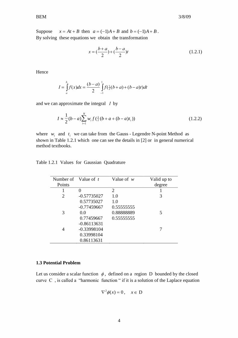
Suppose BAtx then BAa )1( and BAb )1( .

By solving these equations we obtain the transformation

xb a b a

t

( ) ( )2 2

(1.2.1)

Hence

I f x dxb a

f b a b a t dta

b

( )( )

( ( ) ( ) )2

12

1

1

and we can approximate the integral I by

I b a w f b a b a tii

N

i

1

2 1

12( ) ( ( ( ) )) (1.2.2)

where wi and t i we can take from the Gauss - Legendre N-point Method as

shown in Table 1.2.1 which one can see the details in [2] or in general numerical

method textbooks.

Table 1.2.1 Values for Gaussian Quadrature

Number of

Points

Value of t Value of w Valid up to

degree

1 0 2 1

2 -0.57735027

0.57735027

1.0

1.0

3

3

-0.77459667

0.0

0.77459667

0.55555555

0.88888889

0.55555555

5

4

-0.86113631

-0.33998104

0.33998104

0.86113631

7

1.3 Potential Problem

Let us consider a scalar function , defined on a region D bounded by the closed

curve C , is called a “harmonic function “ if it is a solution of the Laplace equation

2 0( )x , x D

BEM 3/8/09

5

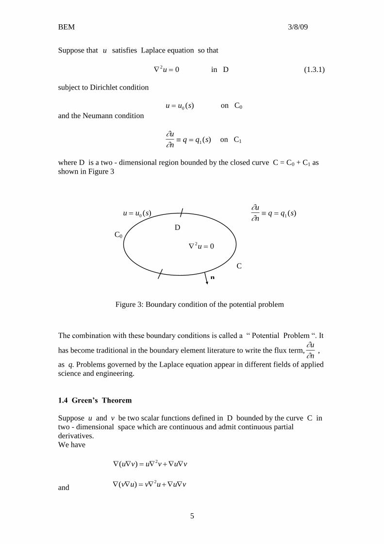
Suppose that u satisfies Laplace equation so that

2 0u in D (1.3.1)

subject to Dirichlet condition

u u s 0 ( ) on C0

and the Neumann condition

u

nq q s 1( ) on C1

where D is a two - dimensional region bounded by the closed curve C = C0 + C1 as

shown in Figure 3

u u s 0 ( )

u

nq q s 1( )

2 0u

The combination with these boundary conditions is called a “ Potential Problem “. It

has become traditional in the boundary element literature to write the flux term,

u

n ,

as q. Problems governed by the Laplace equation appear in different fields of applied

science and engineering.

1.4 Green’s Theorem

Suppose u and v be two scalar functions defined in D bounded by the curve C in

two - dimensional space which are continuous and admit continuous partial

derivatives.

We have

( )u v u v u v2

and ( )v u v u u v2

C0

C

1

D

n

Figure 3: Boundary condition of the potential problem

BEM 3/8/09

6

Taking the difference between these two equations and integrating over D then

DD

dAuvvudAuvvu 22 (1.4.1)

Applying the Gauss Theorem to the left hand side then

CD

uvvudAuvvu .)()( nds

Hence

dsn

uv

n

vudAuvvu

CD

(1.4.2)

Equation (1.4.1) after (1.4.2) we obtain

dsn

uv

n

vudAuvvu

CD

22

(1.4.3)

This is the expression of the well known Second Green Theorem.

1.5 Fundamental Solution of the Laplace Equation

Suppose that R is the position vector of a point, Q, relative to point, P, inside D.

Surround P by a small disc, center P radius , as shown in Figure 4.

Let 0rrR , R = R and u*( R ) is the fundamental solution of the Laplace

equation which satisfies

1qq

0uu

C0

Q R

D P

D

Figure 4: Neighborhood of the point p in the domain D

n

C1

r

0r

BEM 3/8/09

7

(*2 u )0r

where )(r is Dirac delta function which property

0)( r except at 0rr

and D

f ( r )() 0r dA = f )( 0r

We see that

0*2 u

everywhere except at 0r

To find the fundamental solution we first find the solution of the above homogeneous

equation. In cylindrical co-ordinates , by the fact that

22

2 2

2

2

1 1u R

u

R R

u

R R

u** *

( )

and that the solution depends only on the variable R we obtain

01 **2

dR

du

RdR

ud

This ordinary differential equation can be solved easily and then we get

u C R D* ln

Since D is an arbitrary constant we can choose D = 0 and then we obtain

u C R* ln (1.5.1)

To find the constant C we apply the property of Dirac delta function and then

2 1u dA r dA

DD

* ( )

Applying the Divergence Theorem we obtain

C

u*1 .nds dsn

u

C

*

Since

u

n

u

R

R

n

* *

BEM 3/8/09

8

then

u

n

C

R

*

, where n is outward normal

Thus 1 20

2C

RRd C

Finally we have C 1

2

Substituting in (1.5.1) we obtain

u R R*( ) ln 1

2 (1.5.2)

which is the fundamental solution of Laplace equation.

1.6 Integral Equation ( Internal points )

From Figure 4, we apply the Second Green‟s Theorem (1.4.3) with v = u* to the

region D - D then

( ) ( )* **

*u u u u dA uu

nuu

nds

D D C C

2 2

Since both u and u* are harmonic in D - D the integral on the left hand side is zero

therefore

( ) ( )*

**

*uu

nu

u

nds u

u

nu

u

nds

C C

(1.6.1)

Substituting (1.5.2) in (1.6.1) and the fact that

u

nq we have

1

2

1

2

1

20 0

((ln )

ln ) lim ( ln ) lim ( ln )uR

nq R ds u

nR ds q R ds

C C C

In the limit as 0 , since u is continuous with continuous partial derivative then

u up and q qp

Hence

1

2

1

2

1

20 0

((ln )

ln ) lim ( ) lim ( ln )uR

nq R ds u ds q ds

C

p p

C C

BEM 3/8/09

9

Computing the right hand side and using L‟Hospital rule at the last term we obtain

u uR

nq R dsp

C

1

2

(

(ln )ln ) (1.6.2)

or dsnRR

uqRuC

p

.

1()ln(

2

12

(1.6.3)

i.e. u u q uq dsp

C

( )* * , where qu

n

**

(1.6.4)

1.7 Integral Equation ( Boundary Points )

Suppose that P itself is a point on the boundary at which there is a kink with angle

as shown in Figure 5 . If the boundary is smooth at P then = .

This section will illustrate the property of the boundary point . In the similar analysis

as shown in the previous section . We obtain from Figure 6 as

dsn

uu

n

uuds

n

uu

n

uudAuuuu

CCCDD

*

)()()( **

**

2**2

(1.7.1)

Again the left hand side is zero therefore

( ) ( )*

**

*

*

uu

nuu

nds u

u

nuu

nds

C C C

C

P

D

Figure 5

P

1

2

n D

D-D

C-

C Figure 6

C*

BEM 3/8/09

10

Taking limit as 0 then

dsn

uuds

n

uuds

n

uu

n

uu

CCC

**

)(lim)(lim)( *

0

*

0

**

Therefore

1

2

1

2

1

20 01

2

1

2

((ln )

ln ) lim lim ( ln )uR

nq R ds u d q d

C

p p

Computing the right hand side and using L‟Hospital‟s rule at the last term and we

have 2 1 .

So that

u u

R

nq R dsp

C

((ln )

ln ) (1.7.2)

or u R q uRR n dsp

C

( ln ) (

^12

(1.7.3)

i.e. cu u q uq dsp

C

( )* * , where c

2 (1.7.4)

It is clear that if P is an interior point then 2 and hence c 1 . If P is a

boundary point and curve C smooth then therefore c 12 .

BEM 3/8/09

11

2. The Boundary Element Method

This section contains two main objects of this report . The first is concerned with the

fundamental concept of the Boundary Element Method . The second we explain the

spreadsheet implementation and summarize how to implement it. We follow the

notation of Davies and Crann [1].

2.1 Fundamental Concept

We have obtained the integral equation (1.7.2) from the previous section which is the

important tool . This section will apply it to approximate u and q by the Boundary

Element Method as follows.

Suppose that w s j Nj ( ): ,2, ,..., 1 3 is a set of linearly independent function of

position, s, around CN, where, if node j is at the point sj then w si j ij( ) , with the

Kronecker delta function given by

ji

jiij

,0

,1

Then the boundary element approximation to u and q are given by

~( ) ( )

~( ) ( )

u s w s U

q s w s Q

j j

j

N

j j

j

N

1

1

(2.1.1)

We shall choose the nodes to be at the midpoint of the elements and w sj ( ) to be

piecewise constant, yielding the so called “constant element”, with w sj ( ) given by

N 1

2

3 ...

...

C

CN

[N]

[1]

[2]

[3]

[...]

[...]

Figure 7: Partition of the boundary into N elements

BEM 3/8/09

12

otherwise

jssw j

,0

][,1)(

By substituting (2.1.1) into (1.7.2) we have

dsRQswn

RUswU

C

i

N

j

jj

iN

j

jjii

ln))(()(ln

))((11

Hence

N

j

j

C

ij

N

j

j

i

C

jii QdsRswUdsn

RswU

NN11

ln)()(ln

)(

(2.1.2)

where iR |R| and Ri is the position vector of a boundary point relative to node i.

Since w sj ( ) is non-zero only in element [j] , in which it takes value 1 , we can

write equation (2.1.2) as

j

N

j

ijj

N

j

ijii QGUHU

11

ˆ (2.1.3)

where (ln )[ ]

Hn

R dsij

j

ij

(2.1.4)

and G R dsij ij

j

ln[ ]

(2.1.5)

as shown in Figure 8

We see that

target element

base node

[j]

i

dij

jn

Figure 8: Distance from the node i to the element [j]

ijR

BEM 3/8/09

13

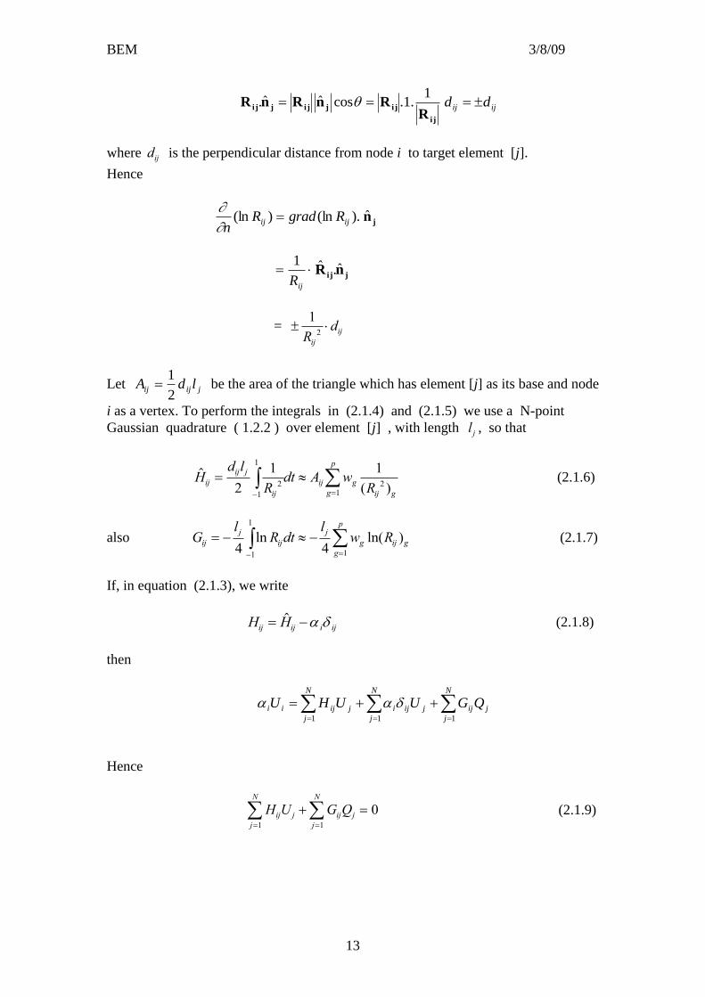
i j

ijjijjijR

RnRnR1

.1.cosˆˆ. ijij dd

where dij is the perpendicular distance from node i to target element [j].

Hence

).(ln)(ln ijij RgradRn

jn

ijR

1jij nR ˆ.ˆ

= 12Rd

ij

ij

Let jijij ldA2

1 be the area of the triangle which has element [j] as its base and node

i as a vertex. To perform the integrals in (2.1.4) and (2.1.5) we use a N-point

Gaussian quadrature ( 1.2.2 ) over element [j] , with length l j , so that

( )

Hd l

Rdt A w

Rij

ij j

ij

ij g

ij gg

p

2

1 12

1

1

21

(2.1.6)

also Gl

R dtl

w Rij

j

ij

j

g

g

p

ij g

4 41

1

1

ln ln( ) (2.1.7)

If, in equation (2.1.3), we write

H Hij ij i ij (2.1.8)

then

j

N

j

ijj

N

j

N

j

ijijijii QGUUHU

11 1

Hence

H U G Qij j

j

N

ij

j

N

j

1 1

0 (2.1.9)

BEM 3/8/09

14

Let H = Hij N N

U = U j N1

G = Gij N N

Q = Qj N1

We can write (2.1.9) in the matrix form as

HU + GQ = 0 (2.1.10)

If i j then Rii and ni are orthogonal , so that R nii i 0

Hence

NiH ii ,...,3,2,1,0ˆ (2.1.11)

For Gii we can integrate analytically to obtain

G lii i

li 1 2ln( ) (2.1.12)

Since u 1 is harmonic in D with 1u and 0q on C , equation (2.1.3)

yields

i ij

j

N

H

1

therefore we obtain

H Hii ij

jj i

N

1

(2.1.13)

When equation (2.1.10) has been solved we know the values of Ui and Qi at all

nodal points. We now use equation (1.7.2) to obtain the solution at k internal

points by the followings.

In a similar manner to which we approximate Hij and Gij for nodal points we can

obtain kjH and kjG for internal points as follows:

H A wR

kj kj g

kj gg

p

12

1 ( ) (2.1.14)

BEM 3/8/09

15

Gl

w Rkj

j

g

g

p

kj g

4 1

ln( ) (2.1.15)

Finally, we obtain the solution for internal points as

U H U G Qk kj j

j

N

kj

j

N

j

1

2 1 1( ) (2.1.16)

BEM 3/8/09

16

2.2 Spreadsheet Implementation

We begin this section with discussing some features in geometry then we summarize

the algorithm of the Boundary Element Method applied in a spreadsheet . Finally we

finish this section by implementing the spreadsheet to solve some potential problems.

Consider the potential problem on the region D with the boundary C in rectangular

co-ordinate as shown in Figure 9

It is clear that if P(x , y) is an arbitrary point then the relationships between co-

ordinate and angle, , are as follows:

x = |OP|cos (2.2.1)

y = |OP|sin (2.2.2)

Let us discuss only on each of those elements, boundary points and internal points

because we can use the facilities of Excel to replicate them easily and we will

describe later.

Suppose that (xi , yi) be the co-ordinate of node i

(xj , yj) be the co-ordinate of node j of element [j]

(xi ,yi)

(xk ,yk) *

* *

*

(Xj ,Yj)

(Xj+1,Yj+1)

I II

II

I (xj ,yj)

O X

Y

P(x , y)

Figure 9: Geometry of the boundary element method

Rkj

Rij

(xg ,yg)

BEM 3/8/09

17

(Xj ,Yj) be the co-ordinate of end point of element [j]

(xk , yk) be the co-ordinate of internal point k

and (xg ,yg) be the co-ordinate of Gauss quadrature point

as shown in Figure 9.

We can easily compute the areas Aij and Akj by using ( 1.1.1) as the following .

A x y X Y X y X y X Y x Yij i j j j j i j i j j i j 1 1 1 1 (2.2.3)

and A x y X Y X y X y X Y x Ykj k j j j j k j k j j k j 1 1 1 1 (2.2.4)

The integration over each element is obtained by using the Gauss-Legendre N-point

method. We have chosen a 3-point rule as shown in Figure 9. By using (1.2.1) we

obtain

tXXxx jjj )(2

11

and tYYyy jjj )(2

11

where the value of t and w we take from Table 1.2.1 as the following

1321

321

,88888889.0,55555555.0:

77459667.0,0.0,77459667.0:

wwwww

tttt

g

g (2.2.5)

So that in element [j] we obtain the Guassian quadrature points as

gjjjg tXXxx )(2

11 (2.2.6)

and gjjjg tYYyy )(2

11 (2.2.7)

Hence

( ) ( ) ( )R x x y yij g i g i g

2 2 2 (2.2.8)

and ( ) ( ) ( )R x x y ykj g k g k g

2 2 2 (2.2.9)

Now we are ready to construct the whole system of linear equation of all elements.

First we obtain Hij by using (2.1.6) and (2.1.11) as

BEM 3/8/09

18

3

1

22 ,)()/(

,0

ˆ

g

igiggij

ij jiyyxxwA

ji

H (2.2.10)

Then we construct Hij by using (2.1.8) and (2.1.13) as

jiH

jiHH

ij

N

i

ij

ij

,ˆ

,ˆ

1 (2.2.11)

and construct Gij by using (2.1.7) and (2.1.12) as

3

1

22 ),)()ln((4

)),2/ln(1(

g

igigg

j

jj

ijjiyyxxw

l

jill

G (2.2.12)

Next we add the Dirichlet and Neumann conditions of the boundary points so that we

have U j and Q j in hand. Consequently we obtain the system of linear equation as

the following.

H U G Q bij N N j N ij N N j N j N

1 1 1 (2.2.13)

By setting bj 0 for j = 1,2,3,...,N by (2.2.10) then using the “ Solver option “ in

Excel we obtain the solutions U j and Q j

Next we construct Hkj by using (2.1.6) as

H A w x x y ykj kj g g k g k

g

/ (( ) ( ) )2 2

1

3

(2.2.14)

and obtain Gkj by using (2.1.7) as

Gl

w x x y ykj

j

g g k g k

g

4

2 2

1

3

ln(( ) ( ) ) (2.2.15)

Finally by using (2.1.16) the interior solution Uk is obtained by

U H U G Qk kj j kj j

j

N

j

N

1

2 11 k = 1,2,3,...,M (2.2.16)

We finish this section by summarizing the process described above in the following

flow chart.

BEM 3/8/09

19

START

Data input

Internal points

(xk , yk)

Boundary points

(xi ,yi)

Computing areas

Aij

End points

(Xj , Yj)

Computing length

lj

Quadrature points

(xg , yg)

Quadrature value

tg and wg

Computing areas

Akj

Constructing matrix

Hij

Constructing matrix

Hkj

Constructing matrix

Hij

Constructing matrix

Gij Constructing matrix

Gij

Dirichlet conditions

U j

Neumann conditions

Q j

Solving equations

HU + GQ = 0

by „ Solver „ option

Boundary solutions

U j and Q j

Internal Solutions

Uk

STOP

BEM 3/8/09

20

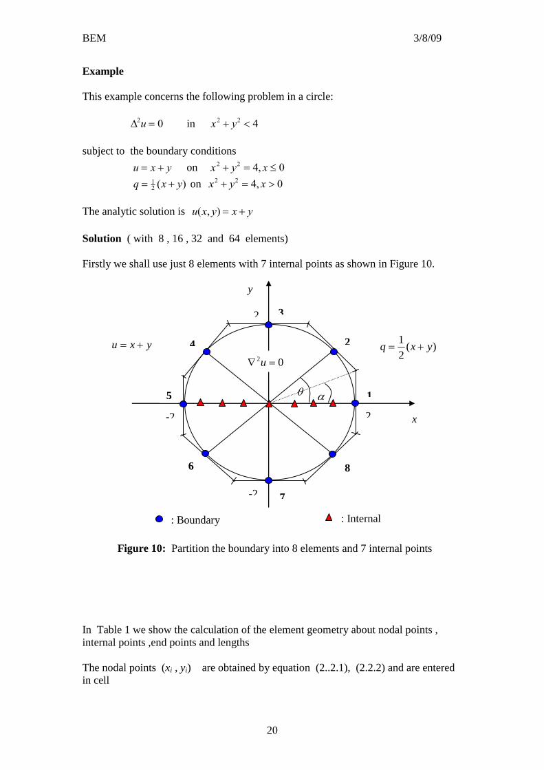
Example

This example concerns the following problem in a circle:

2 0u in x y2 2 4

subject to the boundary conditions

u x y on x y x2 2 4 0 ,

q x y 12 ( ) on x y x2 2 4 0 ,

The analytic solution is u x y x y( , )

Solution ( with 8 , 16 , 32 and 64 elements)

Firstly we shall use just 8 elements with 7 internal points as shown in Figure 10.

In Table 1 we show the calculation of the element geometry about nodal points ,

internal points ,end points and lengths

The nodal points (xi , yi) are obtained by equation (2..2.1), (2.2.2) and are entered

in cell

: Boundary

node

: Internal

point

1

7

6

5

4

3

2

8

yxu )(2

1yxq

y

x

02 u

2

-2

2

-2

Figure 10: Partition the boundary into 8 elements and 7 internal points

BEM 3/8/09

21

B7 (R) as =2*COS((A7-1)*2*PI()/8)

and C7(R) as =2*SIN((A7-1)*2*PI()/8)

The end points (Xj , Yj ) are obtained by the similar way and are entered in cell

H7(R) as =(2/COS(2*PI()/16))*COS((2*A7-3)*(2*PI()/16))

and I7(R) as =(2/COS(2*PI()/16))*SIN((2*A7-3)*(2*PI()/16))

The calculation of co-ordinates of the endpoints and the nodal points are shown in

Table 1..

Table 1: Co-ordinate of nodal points, internal points and endpoints of elements

The length lj of each element we can compute directly by distance formula and are

entered in cell

K7(R) as =SQRT((H7-H8)^2+(I7-I8)^2)

The internal points we firstly choose 7 points as show in Table1.

In Table 2 we show the calculation of areas of triangles from nodal points and

internal points.

BEM 3/8/09

22

The area Aij are obtained by using equation (2.2.3) and are entered in cell

B31(RR) as

=ABS(1/2*(-$B7*B$20-B$19*C$20-

C$19*$C7+B$19*$C7+C$19*B$20+$B7*C$20))

The area Akj are obtained by using equation (2.2.4) and are entered in cell

B42(RR) as

=ABS(1/2*(-$E7*B$20-B$19*C$20-

C$19*$F7+B$19*$F7+C$19*B$20+$E7*C$20))

Table 2: Area of triangles which the vertices are at the nodal points and internal

points

BEM 3/8/09

23

In Table 3 we show weighted value and the calculation of Gauss points .

The Gauss points are given by equations (2.2.6) and (2.2.7) and are enter in cell

C54 .. C56 (R) and C59 .. C61 (R) as follows:

=B24+((C19-B19)/2)*$C$65

and =B25+((C20-B20)/2)*$C$65

Table3 : The weighted values and co-ordinates of the Gauss points

BEM 3/8/09

24

The coefficient matrix Aij are shown in Table 4.

Table 4: The coefficient matrix ijH

We construct the matrix ijH by using equation (2.2.10) and are entered in cell B71

as the following.

=IF($A71=B$70,0,B31*($I$65*((C$54-$B7)^2+(C$59-$C7)^2)^(-

1)+$J$65*((C$55-$B7)^2+(C$60-$C7)^2)^(-1)+$K$65*((C$56-$B7)^2+(C$61-

$C7)^2)^(-1)))

The coefficient matrices Hij , Gij and the boundary solutions are shown in Table 5.

Table 5: The coefficient matrices Hij and Gij

BEM 3/8/09

25

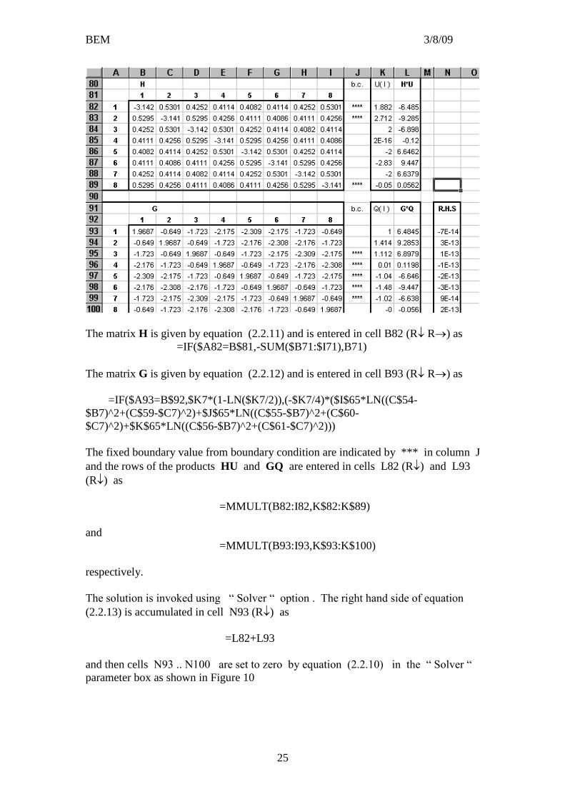
The matrix H is given by equation (2.2.11) and is entered in cell B82 (R R) as

=IF($A82=B$81,-SUM($B71:$I71),B71)

The matrix G is given by equation (2.2.12) and is entered in cell B93 (R R) as

=IF($A93=B$92,$K7*(1-LN($K7/2)),(-$K7/4)*($I$65*LN((C$54-

$B7)^2+(C$59-$C7)^2)+$J$65*LN((C$55-$B7)^2+(C$60-

$C7)^2)+$K$65*LN((C$56-$B7)^2+(C$61-$C7)^2)))

The fixed boundary value from boundary condition are indicated by *** in column J

and the rows of the products HU and GQ are entered in cells L82 (R) and L93

(R) as

=MMULT(B82:I82,K$82:K$89)

and

=MMULT(B93:I93,K$93:K$100)

respectively.

The solution is invoked using “ Solver “ option . The right hand side of equation

(2.2.13) is accumulated in cell N93 (R) as

=L82+L93

and then cells N93 .. N100 are set to zero by equation (2.2.10) in the “ Solver “

parameter box as shown in Figure 10

BEM 3/8/09

26

The result of “ Solver “ process is shown in Figure 11.

Figure 10: The Solver active box

Figure 11: The status of the Solver result

BEM 3/8/09

27

Table 6: The boundary solutions and the matrices kjH and Gkj

The matrix kjH is given by equation (2.1.14) and is entered in cell B116 (R R)

as

=B105*($I$65*((C$54-$E7)^2+(C$59-$F7)^2)^(-1)+$J$65*((C$55-

$E7)^2+(C$60-$F7)^2)^(-1)+$K$65*((C$56-$E7)^2+(C$61-$F7)^2)^(-1))

The matrix Gkj is given by equation (2.2.15) and is entered in cell B126 (R R)

as

=(-$K7/4)*($I$65*LN((C$54-$E7)^2+(C$59-$F7)^2)+$J$65*LN((C$55-

$E7)^2+(C$60-$F7)^2)+$K$65*LN((C$56-$E7)^2+(C$61-$F7)^2))

Finally the internal solution Uk is given by equation (2.2.16) and is entered in cell

G143 (R)

=(L117+L128)/(2*PI())

as shown in Table 7.

BEM 3/8/09

28

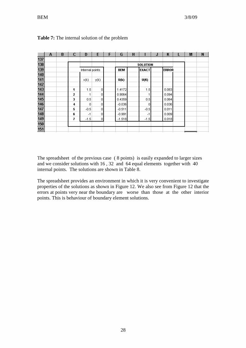
Table 7: The internal solution of the problem

The spreadsheet of the previous case ( 8 points) is easily expanded to larger sizes

and we consider solutions with 16 , 32 and 64 equal elements together with 40

internal points. The solutions are shown in Table 8.

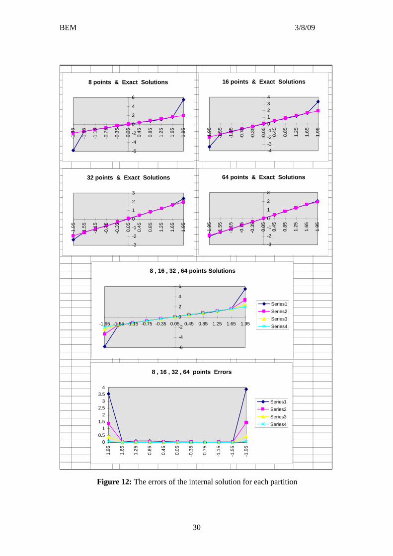
The spreadsheet provides an environment in which it is very convenient to investigate

properties of the solutions as shown in Figure 12. We also see from Figure 12 that the

errors at points very near the boundary are worse than those at the other interior

points. This is behaviour of boundary element solutions.

BEM 3/8/09

29

Table 8: The internal solutions of 8, 16, 32 and 64 elements with 40 internal points.

Solutions by N-nodal points Exact Errors in each case

Solution

Internal points 8 16 32 64 u = x + y 8 16 32 64

x(k) y(k) U(k) U(k) U(k) U(k) u(k)

1 1.95 0 5.494 3.325 2.352 2.013 1.95 3.544 1.375 0.402 0.063

2 1.85 0 2.5 1.975 1.854 1.848 1.85 0.65 0.125 0.004 0.002

3 1.75 0 1.906 1.743 1.741 1.747 1.75 0.156 0.007 0.009 0.003

4 1.65 0 1.645 1.62 1.64 1.648 1.65 0.005 0.03 0.01 0.002

5 1.55 0 1.482 1.515 1.54 1.548 1.55 0.068 0.035 0.01 0.002

6 1.45 0 1.358 1.415 1.441 1.448 1.45 0.092 0.035 0.009 0.002

7 1.35 0 1.249 1.316 1.341 1.348 1.35 0.101 0.034 0.009 0.002

8 1.25 0 1.147 1.218 1.242 1.248 1.25 0.103 0.032 0.008 0.002

9 1.15 0 1.05 1.12 1.142 1.148 1.15 0.1 0.03 0.008 0.002

10 1.05 0 0.954 1.022 1.042 1.048 1.05 0.096 0.028 0.008 0.002

11 0.95 0 0.859 0.923 0.943 0.948 0.95 0.091 0.027 0.007 0.002

12 0.85 0 0.765 0.825 0.843 0.848 0.85 0.085 0.025 0.007 0.002

13 0.75 0 0.671 0.727 0.744 0.748 0.75 0.079 0.023 0.006 0.002

14 0.65 0 0.577 0.628 0.644 0.649 0.65 0.073 0.022 0.006 0.001

15 0.55 0 0.483 0.53 0.545 0.549 0.55 0.067 0.02 0.005 0.001

16 0.45 0 0.389 0.432 0.445 0.449 0.45 0.061 0.018 0.005 0.001

17 0.35 0 0.295 0.333 0.346 0.349 0.35 0.055 0.017 0.004 0.001

18 0.25 0 0.2 0.235 0.246 0.249 0.25 0.05 0.015 0.004 0.001

19 0.15 0 0.106 0.137 0.146 0.149 0.15 0.044 0.013 0.004 1E-03

20 0.05 0 0.011 0.038 0.047 0.049 0.05 0.039 0.012 0.003 9E-04

21 -0.05 0 -0.08 -0.06 -0.05 -0.05 -0.05 0.033 0.01 0.003 8E-04

22 -0.15 0 -0.18 -0.16 -0.15 -0.15 -0.15 0.028 0.009 0.002 7E-04

23 -0.25 0 -0.27 -0.26 -0.25 -0.25 -0.25 0.023 0.007 0.002 6E-04

24 -0.35 0 -0.37 -0.36 -0.35 -0.35 -0.35 0.018 0.006 0.002 5E-04

25 -0.45 0 -0.46 -0.45 -0.45 -0.45 -0.45 0.013 0.005 0.001 4E-04

26 -0.55 0 -0.56 -0.55 -0.55 -0.55 -0.55 0.009 0.003 0.001 3E-04

27 -0.65 0 -0.65 -0.65 -0.65 -0.65 -0.65 0.004 0.002 7E-04 2E-04

28 -0.75 0 -0.75 -0.75 -0.75 -0.75 -0.75 5E-05 9E-04 3E-04 1E-04

29 -0.85 0 -0.85 -0.85 -0.85 -0.85 -0.85 0.004 3E-04 2E-05 4E-05

30 -0.95 0 -0.94 -0.95 -0.95 -0.95 -0.95 0.007 0.002 3E-04 4E-05

31 -1.05 0 -1.04 -1.05 -1.05 -1.05 -1.05 0.01 0.003 6E-04 1E-04

32 -1.15 0 -1.14 -1.15 -1.15 -1.15 -1.15 0.012 0.004 9E-04 2E-04

33 -1.25 0 -1.24 -1.25 -1.25 -1.25 -1.25 0.011 0.005 0.001 3E-04

34 -1.35 0 -1.34 -1.34 -1.35 -1.35 -1.35 0.006 0.006 0.001 3E-04

35 -1.45 0 -1.46 -1.44 -1.45 -1.45 -1.45 0.006 0.006 0.002 4E-04

36 -1.55 0 -1.59 -1.54 -1.55 -1.55 -1.55 0.036 0.005 0.002 5E-04

37 -1.65 0 -1.76 -1.65 -1.65 -1.65 -1.65 0.106 4E-04 0.002 5E-04

38 -1.75 0 -2.03 -1.78 -1.75 -1.75 -1.75 0.282 0.025 0.001 6E-04

39 -1.85 0 -2.66 -2.01 -1.86 -1.85 -1.85 0.81 0.16 0.012 2E-04

40 -1.95 0 -5.84 -3.38 -2.36 -2.02 -1.95 3.888 1.432 0.412 0.065

BEM 3/8/09

30

8 points & Exact Solutions

-6

-4

-2

0

2

4

6

1.9

5

1.6

5

1.2

5

0.8

5

0.4

5

0.0

5

-0.3

5

-0.7

5

-1.1

5

-1.5

5

-1.9

5

16 points & Exact Solutions

-4

-3

-2

-1

0

1

2

3

4

1.9

5

1.6

5

1.2

5

0.8

5

0.4

5

0.0

5

-0.3

5

-0.7

5

-1.1

5

-1.5

5

-1.9

5

32 points & Exact Solutions

-3

-2

-1

0

1

2

3

1.9

5

1.6

5

1.2

5

0.8

5

0.4

5

0.0

5

-0.3

5

-0.7

5

-1.1

5

-1.5

5

-1.9

5

64 points & Exact Solutions

-3

-2

-1

0

1

2

3

1.9

5

1.6

5

1.2

5

0.8

5

0.4

5

0.0

5

-0.3

5

-0.7

5

-1.1

5

-1.5

5

-1.9

5

8 , 16 , 32 , 64 points Solutions

-6

-4

-2

0

2

4

6

1.951.651.250.850.450.05-0.35-0.75-1.15-1.55-1.95

Series1

Series2

Series3

Series4

8 , 16 , 32 , 64 points Errors

0

0.5

1

1.5

2

2.5

3

3.5

4

1.9

5

1.6

5

1.2

5

0.8

5

0.4

5

0.0

5

-0.3

5

-0.7

5

-1.1

5

-1.5

5

-1.9

5

Series1

Series2

Series3

Series4

Figure 12: The errors of the internal solution for each partition

31

References

Brebbia, C.A. (1978) The boundary element method for engineers, London: Pentech

Press.

Chiskawski, R.D. and Brebbia, C.A. (1991) Boundary element method in acoustics,

Addison-Wesley.

Colley, S.J. (1998) Vector Calculus, Prentice-Hall.

Davies, A.J. (1980) The finite element method: A first approach, Oxford University

Press.

Davies, A.J. and Crann, D. (1996) Using a spreadsheet for the boundary element

method: Interior and exterior problems. 13, Mathematics Department:

University of Hertfordshire.

Gerald, C.F. and Wheatley, P.O. (1994) Applied numerical analysis, Addison-

Wesley.

Humi, M. and Miller, W.B. (1992) Boundary value problems and patial differential

equation, PWS-KENT.

Paris, F. and Canas, J. (1997) Boundary element method: Foundations and

Application, Oxford: Oxford University Press.

====================================