study of the temporal behavior of gps/galileo nse...

Study of the Temporal Behavior of GPS/GALILEO NSE and RAIM for LPV200

Pierre NERI, AIRBUS, France Laurent AZOULAI, AIRBUS, France

Christophe MACABIAU, ENAC, France

BIOGRAPHIES

Pierre NERI graduated as an electronics engineer in 2007 from the ENAC (Ecole Nationale de l’Aviation Civile) in Toulouse, France. Since 2007, he is a Ph.D student at the signal processing lab of ENAC working on multi constellation GNSS receivers for civil aviation.

Laurent AZOULAI graduated in 1996 of Institut Supérieur de l’Electronique de Paris as an engineer specialized in automatic systems. He is GNSS-Landing Systems Technical Expert with Airbus Design Office. His activities focus on future Approach and Landing Architectures for Airbus aircraft and the foreseen extended use of GNSS in Communication, Navigation and Surveillance aircraft systems. He is involved in standardization activities dealing with GBAS Cat 2/3, GPS/Galileo combination and SBAS for which he is co-chairman of RTCA SC-159 SBAS Working Group.

Christophe MACABIAU graduated as an electronics engineer in 1992 from the ENAC in Toulouse, France. Since 1994, he has been working on the application of satellite navigation techniques to civil aviation. He received his Ph.D in 1997 and has been in charge of the signal processing lab of ENAC since 2000.

ABSTRACT

For many years, civil aviation has identified GNSS as an attractive means to provide navigation services for every phase of flight due to its wide coverage area. However, to do so, GNSS must meet stringent requirements in terms of accuracy, integrity, availability and continuity. To achieve this performance, augmentation systems have been developed to correct the GPS L1 C/A and to monitor the quality of the received Signal-In-Space (SIS). Different solutions exist depending on where and how the augmentation is implemented. We can distinguish ABAS (Aircraft Based Augmentation Systems), SBAS (Satellite Based Augmentation System) and GBAS (Ground Based Augmentation System). ABAS systems are very interesting as they are autonomous, meaning that no signal external to the aircraft is needed to monitor the SIS thereby reducing the dependency on a ground navaids network. It uses redundant information within GNSS constellation to provide integrity monitoring. It is important to note that unlike other augmentation systems,

ABAS does not improve position accuracy. Two types of ABAS systems can be distinguished: Receiver Autonomous Integrity Monitoring (RAIM) where only GNSS information is used, Aircraft Autonomous Integrity Monitoring (AAIM) where information from other on-board sensors is also used. This paper will study the RAIM temporal behavior.

Today RAIM and/or AAIM are commonly used to provide integrity monitoring for phases of flight down to Non Precision Approaches using GPS L1 C/A measurements. However, current performance associated with GPS L1 and GPS constellation is not sufficient to meet civil aviation requirements for more stringent phases of flight and in particular, the associated vertical requirements of APV and LPV200. The introduction of new signals and constellations - such as GPS L5 and GALILEO for example - will significantly increase the number of available signals and satellites, the quality of the measurements as well as the quality of constellation geometries. Thus, RAIM may provide a simple means to monitor the quality of the SIS and to reach more stringent phases of flight such as approaches with vertical guidance like APV or LPV200 operations.

This possibility has been investigated by the civil aviation community during recent years and RAIM is now foreseen as an interesting candidate to provide integrity monitoring for LPV200. Different algorithms have been studied and their performance, in terms of availability, has been published. It results that RAIM alone does not appear to provide sufficient protection for LPV200 approaches. New possibilities to extend RAIM to APV and LPV200 are under study and it can be reasonably assumed that RAIM using GPS and GALILEO constellations could be used in the near future (Advanced RAIM). Therefore, it appears necessary to address the specific phenomena that will result from the combination of two different constellations in one positioning solution. The aim of this paper is to present a microscopic analysis of the temporal behavior of GPS and GALILEO Navigation System Error (NSE) and RAIM, under various constellations and signal configurations for LPV200 types of operation. Indeed, the use of different types of satellites, the constellation changes, the potential loss of frequencies may imply unexpected behavior of NSE. Thus, the impact of the introduction of this new positioning solution must be investigated so as to limit

3796

unwanted effects for aircraft flight control systems which use the GNSS computed position. To enable this study to take place, a GPS/GALILEO + RAIM receiver model has been developed.

The first section is a presentation of the receiver model used for the simulations which is composed of the following different modules: an aircraft trajectory generator, the measurement error models, the receiver model, the Position Velocity Time (PVT) module and the integrity monitoring (only RAIM will be used in this study). The receiver model is based on a correlator outputs generator able to model different receiver configurations for several signals and constellations. The error models used as well as the inputs and outputs of the simulator are described. The Least Square Residuals (LSR) RAIM algorithm is also detailed. The second section describes the study case defined for our simulations including various configurations of constellations, signals and approaches as well as the spatial and temporal grid used to evaluate the behavior of NSE. The following section provides a microscopic study of the position error time behavior when using GPS and GALILEO dual frequency, and in the presence of constellation changes. Aircraft maneuvers along the approach will be considered so as to observe their impact on the error. For example, a sharp turn can result in the loss of a satellite due to the antenna pattern. The next section discusses the benefits of using special configurations with respect to the additional complexity and errors introduced. The typical example to study is the resulting benefits from using single frequency on one constellation and dual frequency on the other. On the one hand, additional satellites provide a better geometry but on the other hand single frequency measurements are far less accurate than dual frequency measurements and will therefore introduce additional errors in the positioning solution. This section also investigates the impact of unbalanced numbers of satellites in the two different constellations. Finally, the last section of this paper studies the possibility of using methods such as constellation prediction to prevent unwanted NSE behaviors.

I. INTRODUCTION

Nowadays, ABAS are commonly used onboard civil aviation aircraft to monitor the quality of the GPS L1 C/A signal, allowing using GNSS as a primary means of navigation for phases of flight from oceanic down to NPA. However, the performance of the current ABAS position solutions does not allow extending their use to more stringent phases of flight and in particular, it cannot guarantee sufficient levels of performance in terms of vertical guidance. However, ABAS solutions are very attractive since they do not need the support of external infrastructures to be operational, which allows to take benefit from the actual worldwide coverage of the GNSS constellations. Thus, the possibility to develop enhanced ABAS position solutions supporting more demanding

phases of flight such as APV and CAT-I would be an important breakthrough for civil aviation users.

The introduction of new GNSS constellations such as GALILEO as well as new GNSS signals such as GPS L5 is an opportunity to develop new GNSS receivers including dual-frequency or even dual constellation capabilities. In this context, Civil Aviation community foresees ABAS as an interesting candidate to provide integrity monitoring to these receivers. It is thus an opportunity to combine the advantages of ABAS with the increased performance raised by new constellations, new satellites and new signals so as to reach more stringent SIS requirements.

However, it appears necessary to address the specific phenomena that will result from the combination of two different constellations in one positioning solution. The aim of this chapter is thus to present an analysis of the temporal behavior of GPS and GALILEO combined position solution augmented by RAIM. A particular focus is put on the impact of constellation changes on the position error. Moreover a simple algorithm is proposed to limit this impact during the final part of GNSS approaches.

II. RECEIVER MODEL II.1. Introduction

So as to study the behavior of the GPS and GALILEO NSE with RAIM, it was necessary to develop a receiver simulator which would reliably represent the behavior of a real receiver. Of course the best way to do so would have been to develop a complete simulated software receiver but the amount of simulations necessary to obtain results imply a too huge computational burden. Therefore the solution was to choose a tradeoff between the fidelity of our model and the associated time consumption. We decided to develop a Correlator Outputs generator which instead of generating the whole sampled GNSS signals at the input of the receiver signal processing directly generate the correlator outputs depending on the carrier phase and code phase estimation errors. This solution combines many advantages:

- Easier generation of errors affecting the pseudorange measurements

- Versatility due to a modular architecture composed of several models

- Reduced computational burden and time consumption

- High fidelity of the behaviour of the receiver signal processing

We now present the architecture of the whole simulator including the receiver model. The different models are described and detailed.

3797

II.2. Simulator Architecture

As previously explained, the simulator is composed of several modules which can be separated in four categories:- Environmental models: these are the models

concerning the phenomena external to the receiver and which determine the pseudorange behaviour

- Receiver signal processing: It gathers the models representing elaboration of the pseudorange measurement which are mainly the tracking loops.

- Position computation and monitoring: It contains the models used to compute a position using the GNSS measurements and the associated integrity monitoring.

- Error models: models of each error affecting the pseudorange measurements.

We can notice here that errors affecting GNSS measurements are generated at different levels of this architecture since, depending on the type of errors, it is easier to model the associated impact at a different level of the simulator.

Figure 1: Simulator Architecture

II.3. Environment models

Trajectory generator

A trajectory generator has been developed so as to define the reference position of the aircraft during a RNAV/GNSS approach. This module was developed using as a basis the RNAV/GNSS procedure for Lille Lesquin airport, north of France. This type of approaches has standardized “Y” and “T” shapes. The behavior of the aircraft along its trajectory has been taken into account meaning that the attitude of the aircraft is modeled. Of course, it is also possible to use a real trajectory at the input of the simulator.

Satellite simulation

GPS and GALILEO satellites positions and velocities are computed using the GPS and GALILEO almanacs algorithms. The 24 satellites constellation is considered for GPS and 27 in the case of GALILEO. We used the YUMA almanacs format. The almanacs algorithm and structure can be found in [ARINC, 2004].

Distance generation

Thanks to the two previous models it is possible to build the geometrical distance between the simulated aircraft and a GNSS satellite :

Where: - is the position of satellite - is the receiver position

II.4. Signal processing models

Correlator outputs generation

We present here the correlator outputs generator principle. For clarity we will consider here a single channel model and we will focus on the GPS L1 C/A signal. This channel is composed of the code and carrier tracking loops which are the DLL and the PLL. The principle here is to build directly the correlator outputs. Therefore, we can remind here the correlator outputs expressions in the case of Early, Prompt and Late correlators and in the presence of noise only [SPILKER, 1996]:

Where: - are the in-phase correlator outputs - are the quadra-phase correlator

outputs - is the amplitude of the received signal - is the navigation data bit - is the correlation of the locally generated

spreading code with the filtered incoming spreading code

- are respectively the code and carrier phase

tracking error - the Doppler error

- are the correlated noise

for each correlator outputs.

Each parameter above mentioned can be computed since their theoretical expressions are known. As an example the structure of the simulated DLL is presented in the following figure:

TrajectoryGenerator

•GNSSapproachsimulation•Externalsoftware

DistanceGenerator

•Constellationsimulation•Visibility test•Distancecomputation

PVTWeighted Least

Squares

•GPS•GALILEO

•GPS/GALILEO

IntegrityMonitoring

RAIM LSR:•GPS

•GALILEO•GPS/GALILEO

IQ generator

•Correlator outputs generation•Discriminator outputs

generation•Feedback computations

•Noise and multipathgeneration

Pseudorangemeasurement

error

•Residual errorsigma computation

•Residual errorgeneration•Sigma UEREcomputation

Truedistance

MeasuredPseudodistance

Correctedmeasurements

ErrormodelsTroposphere, Ionosphere, Ephemeris, Multipath, Noise, User and

Satellite clocks

SimulatedPseudodistance

Corrections(Ionosphere,Troposphere,Sat clocks )

IQgeneratorinputs(noise,

multipath)

Errors(Ionosphere,Troposphere,

Clocks)

UERE sigmas

A/Ctrueposition

PositionVelocity

HPLVPL

3798

Figure 2: Structure of the simulated DLL

As we can see, the approach is therefore to generate the received code and carrier phase, to generate the locally generated code and carrier phase and to compute the corresponding correlator outputs. After that, the process is the classical one: a discrimination function is used, its output is filtered by the loop filter so as to obtain a command. This command is then turned into the estimated code phase.

Autocorrelation functions

In the simulator, sampled versions of the autocorrelation functions of each available signal are stored. Correlation values are then obtained by linearly interpolating these sampled versions.

Discriminators

The following discriminators have been considered for the DLL:

- Dot-Product (DP):

- Early Minus Late Power (EMLP):

For the PLL we considered the following: - Costas:

- Atan:

- Atan2 :

Loop filters

The outputs of the discriminators are filtered so as to build a command to the VCOs which control the locally generated replicas of the code sequence as well as the carrier of the signal. In this simulator we used the implementation of digital filters presented in [STEPHENS, 1995].

Error models

The pseudorange measurements made by a receiver model for a given satellite at epoch can be written as:

Where: - is the pseudorange measurement - is the geometrical distance between the

receiver and the satellite .- is the ionospheric propagation delay in

seconds. - is the tropospheric propagation delay in

seconds.

- is the code pseudorange measurement error induced by multipath propagation.

- is the code pseudorange measurement noise error

We present in the next sections the different error models that we used to accurately model these measurements.

Ionospheric delay

To generate the total ionospheric delay we used the Klobuchar algorithm which is used in single frequency GPS receivers for ionospheric delay correction. It is well known that this algorithm does not accurately represent the ionospheric delay but the advantage is that it is simple to use and the input parameters can easily be found. The Klobuchar algorithm is described in [ARINC, 2004].

Tropospheric delay

The impact of the propagation of GNSS signals through troposphere is a well known phenomenon and it can be modelled quite efficiently. The model used in GPS receivers so as to correct the tropospheric delay can be found in [RTCA, 2006]. Moreover, GALILEO receivers are supposed to apply a tropospheric correction which is at least as good as the above mentioned [EUROCAE, 2007]. This model is thus considered as a reference for both receivers and that’s why we used it to generate the tropospheric delay affecting the received signals. It can be written as:

Where: - is the estimated vertical range delay (i.e. for

a satellite at 90° elevation angle) induced by gases in hydrostatic equilibrium in meters

- is the estimated vertical range delay caused by water vapor in meters

- is a mapping function that scales the delays to the actual satellite elevation angle

3799

The detailed computation of the parameters of this model can be found in [RTCA, 2006].

Clock errors

To model the errors induced by satellite and receiver clocks we used the stochastic differential equation for Allan variance computation presented in [WINKEL, 2000]. Examples of parameters for different clock types are given in the following table:

Oscillator Whitefrequencynoise

Flicker Integratedfrequencynoise

Standardquartz

2.10 19 s 7.10 21 s 2.10 20 Hz

TCXO 1.10 21 s 1.10 20 s 2.10 20 HzOCXO1 8.10 20 s 2.10 21 s 4.10 23 HzOCXO2 2.51.10 26 s 2.51.10 23

s2.51.10 22 Hz

Rubidium1 2.10 20 s 7.10 24 s 4.10 29 HzRubidium2 1.10 23 s 1.10 22 s 1.3.10 26 HzCesium1 1.10 19 s 1.10 25 s 2.10 32 HzCesium2 2.10 20 s 7.10 23 s 4.10 29 Hz

Table 1: Parameters for the Allan variance of several oscillators [WINKEL, 2000]

Noise

We presented previously the expressions of the correlator outputs and in particular the presence of correlated noises. These correlated noises have a known expression and it is therefore easier for us to generate directly the noise at the level of the correlator outputs. The method used is described in [JULIEN, 2005] and is based on [HURST, 1972]. A vector of correlated noises can be written:

With - the vector of correlated Gaussian noises - a positive definite matrix representing the

expected correlation between noise - the vector of the eigenvectors of - is the diagonal matrix containing the

eigenvalues of so that

In the case of the correlator outputs generation, the expected correlation between each noise is exactly given by the filtered autocorrelation function. Therefore, in the case of early, late and prompt correlators we have for the in-phase components [JULIEN, 2005]:

Where: - is the correlation of the locally generated

spreading code with the filtered incoming spreading code

- is the early-late chip spacing

C is positive definite as required to use the proposed algorithm. All that is left to do is to compute the eigenvectors, the eigenvalues and generate Gaussian noise. The appropriate variance is applied to the noise depending on the simulated signal to noise ratio.

Multipath error

This section addresses the multipath during aircraft approaches. Since multipath is a replica of the signal and since the correlation is a linear process, the expressions presented for the correlator outputs can be used to compute the impact of multipath. For example, if we consider a particular multipath which is characterized by its relative delay , amplitude and phase with respect to the direct signal, we can derive its impact on the in-phase early correlator output for example:

The correlator output in presence of multipath will then be the sum of the direct signal and multipath contributions. This process can be generalized to several multipath.

However, now that we know how to model the impact of multipath on measurements, the difficulty is to realistically model multipath which is difficult since it is dependent on the geographic environment. Our proposed solution is the one used in [MACABIAU, 2006]. They used a model called High Resolution Aeronautical Channel which was initially developed by the DLR for ESA and which allows to generate the multipath affecting the measurements of a receiver aboard an aircraft in approach. This model was presented in [STEINGASS, 2004]. In particular three multipath are generated: - Path 1 : refractive component of the direct path - Path 2: Strong echo on the fuselage that is changing

very slowly - Path 3: Quickly changing ground echo

II.5 Position and Integrity models

RAIM Fault-free Pseudorange measurement model

We assume that pseudorange measurement error components have normal distributions with zero mean.

3800

This section details the computation of the sigma UERE (User Equivalent Range Error) which represents the error budget made for position determination and integrity monitoring. It is the result of the aggregation of the different sources of errors which impacts the pseudorange measurements:

Troposphere

We previously presented the model used by GPS and GALILEO civil aviation users to correct tropospheric error. The error residual error associated to this model is well known and can be written [RTCA, 2006]:

With: - the tropospheric vertical error - is a mapping function that scales the delays to

the actual satellite elevation angle

Ionosphere

For ionospheric error, different cases have to be taken into account. In the nominal mode, future civil aviation GNSS receivers will perform dual frequency measurements. However, single frequency measurements will be used as degraded modes when necessary.

In the case of dual frequency measurements, the receiver can combine the two measurements to obtain a iono-free measurements. This correction allows removing most of the ionospheric delay and therefore the residual error is considered as negligible:

In the case of single frequency measurements we have distinguished GPS and GALILEO satellites since their users will correct the ionospheric error using a different algorithm. In the case of GPS, the Klobuchar algorithm is used. The residual error is well known and can be written [RTCA, 2006]:

Where: - C is the speed of light in a vacuum - is the klobuchar ionospheric correction - is the obliquity factor

-

- is the geomagnetic latitude

In the case of GALILEO, the NeQuick model will be used. As stated in [SALOS, 2010], the error of this model is specified to not exceed 30% of the current ionospheric delay or the equivalent delay caused by a TEC (Total Electron Content) of 20 TECu whichever is larger:

It is then possible to substitute the ionospheric delay with its first order approximate to obtain:

Where: - VTEC is the vertical TEC - is the obliquity factor

In [SALOS, 2010], numerical values of the residual ionospheric delay have been derived using the International GNSS Service (IGS) Vertical TEC database. We used these results in our model.

Receiver noise residual error

The receiver noise residual error is directly linked to the tracking loops error. BETZ formulas give an estimate of the code tracking loop error variance for dot product and EMLP discriminators and considering an ideal rectangular RF filter. They can be found in [BETZ, 2000].

Where: - is the RF front-end filter bandwidth

- is the signal-to-noise ratio of the processed

signal - is the power spectral density of the

processed signal

However, to obtain the final noise variance, we have to take into account two more processes. The first one is only applicable in the case of dual frequency measurements. In this case, by combining two different measurements the variance of noise is increased. In fact dual frequency measurements can be written:

Where: - is the pseudorange measurement at frequency

- is the pseudorange measurement at frequency

We can see here that noise components on each frequency will be combined and affected by a coefficient dependent on the two frequencies. Therefore in our case we obtain:

3801

Finally, we also have to take into account the code carrier smoothing of 100 s which is mandatory for civil aviation receivers used for approach. The impact of the smoothing constant on the variance of the pseudorange measurement can be written as [HEGARTY, 2006]:

Where: - is the time smoothing constant in

seconds - is the raw code pseudorange measurement

error variance

- is the smoothed ode pseudorange measurement error variance

Multipath

The characterization of multipath error for aircraft and for GPS L1 C/A has been tackled by RTCA. This study resulted in a standard curve which has been adopted in ICAO SARPS and is therefore the reference. It described the smoothed multipath error variance. It can be found in [RTCA, 2006]:

This model is also used for other GNSS signals since it is supposed to be conservative with respect to future signals performance concerning resistance to multipath. In the case of duals frequency measurements, the multipath error is affected in the same way as the noise and therefore the same expressions are applied.

Satellite clock and ephemeris uncertainty:

Satellite clock and ephemeris uncertainty will depend on the considered system. For GPS users, the User Range Accuracy (URA) is the standard deviation of the range component of clock and ephemeris uncertainty.

In the case of GALILEO, the Signal In Space error of each satellite is over bounded by a nonbiased Gaussian distribution with a minimum standard deviation called Signal In Space Accuracy (SISA). It can be considered as an equivalent to GPS URA [MARTINEAU, 2008]. The integrity performance requirements specify a SISA value of 85 cm for both nominal and degraded modes in [ESA, 2005].

GPS URA depends on the modernization step of the GPS constellation. For our study, we considered future GNSS constellations and therefore assumed that both GPS and GALILEO satellites will achieve at least a URA of 85 cm:

RAIM Faulted Pseudorange measurement model

The GPS Standard Positioning Service Performance Standard [GPS SPS, 2008] specifies two parameters regarding the satellite integrity: the definition of a major service failure and the specification of the maximum rate of such a satellite fault.

A major service failure is defined to be a condition during which a healthy SPS SIS’s instantaneous URE exceeds the SIS URE NTE tolerance without a timely alert being provided [GPS SPS, 2008]. The NTE SPS SIS URE tolerance for a healthy SPS SIS is defined to be

times the upper bound on the URA value corresponding to the URA index currently broadcast by the satellite [GPS SPS, 2008]. The probability of occurrence of such an event is 3 per year for a 24 GPS satellites constellation.

III. COMBINED GPS/GALILEO POSITION

In this study, the chosen approach was to combine GPS and GALILEO at the pseudorange level. Even if United States and European Union have agreed to provide the GPS to GALILEO Time Offset GGTO through each system’s navigation signals, the determination of this offset is thought not to be part of a safety-critical chain [HAHN, 2005]. Thus, combined GPS-GALILEO receivers will have to solve the offset between the local receiver clock and GPS system time as well as the offset between the local receiver clock and GALILEO system time.

For the position solution it results in taking into account an additional bias in the state vector:

Where: are the Cartesian coordinates of the

antenna phase center of the user receiver is the user receiver GPS clock bias defined by

and is the time offset between the receiver clock and GPS system time

is the user receiver GALILEO clock bias defined by and is the time offset between the receiver clock and GALILEO system time

The impact on the observation matrix is the addition of a fifth column to account for the dependency of pseudorange measurements on which is given by (using the same notations as presented in Chapter 4):

For GPS pseudorange measurement :

3802

For GALILEO pseudorange measurement :

The final observation matrix, assuming GPS pseudorange measurements and GALILEO pseudorange measurements, can be written as:

Of course, this fifth variable to be estimated is taken into account in RAIM equations mainly through the use of this adapted observation matrix. Moreover, for LSR RAIM, the sum of the squares of the pseudorange residuals are considered as chi-squared distributed with

degrees of freedom, instead of (N being the total number of pseudorange measurements used for position computation with ).

IV. CONSTELLATION FREEZING ALGORITHM

The objective of this simple algorithm is to avoid constellation changes during the final part of the approaches, which we have defined as the part of the approach starting at the Final Approach Fix and terminating when the aircraft has successfully landed. Indeed, during automatic approaches and landing phases, it is desirable to avoid any step that would potentially degrade the performance of guidance performance such that it eventually degrades the touchdown performance and could lead to a missed approach.

To implement this algorithm we have assumed that the aircraft knows a sufficiently accurate estimate of its ETA (Estimated Time of Arrival) at the Final Approach Fix (FAF) of the simulated approach and at the touchdown. In fact, we know that most commercial aircraft are equipped with a Flight Management System which provides quite accurate predictions. The accuracy of these predictions increases when getting closer to the point concerned by the predictions. Thus, this assumption can be considered as realistic. However, further studies are needed to

evaluate the level of accuracy of these predictions needed to ensure the efficiency of the proposed algorithm. We also assume that the aircraft is able to estimate the time at which the approach can be considered as terminated. We denote the ETA of the aircraft at the FAF and

the ETA of the end of the approach.

Since the aircraft can only compute imperfect estimates of and and to increase robustness with our computation simplification, we also defined two margins

and around this time interval. Thus, in reality, the aim of the algorithm is to avoid constellation changes on the time interval:

Additionally, we consider that aircraft is flying final approach when .

The core of the algorithm consists in predicting set time of each satellite of the GPS or GALILEO constellations, which is tracked by the receiver before . The computed set times are only estimates which explains why we provisioned margins around the period of interest. The computation of the prediction is detailed hereafter.

It is based on a simple linear extrapolation of the satellites elevation during the end of the approach. We can compute the slope of the linear extrapolation of the satellite elevation as:

Where: is the current elevation angle of satellite

at epoch . is the current time

We want to know at which time the satellite will set, that is to say we want to know at which time the satellite elevation angle will be equal to the considered mask angle:

This prediction allows identifying which satellites may lead to a constellation change during the final approach when:

Thus, it is possible to remove all these satellites from the position solution before entering the final approach phase so as to ensure that no constellation change will occur between the moment the aircraft is flying the FAF and the moment the aircraft has successfully landed. To do so, we also have to inhibit inclusion of rising satellites in the position solution after .

3803

In fact, this reasoning is based on the assumption that since we are using a combined GPS-GALILEO receiver, it is likely that even if we remove some of the available satellites from the position solution, there will be far enough visible satellites left to compute an accurate position. It remains interesting to compare the degradation of accuracy due to the reduction of the number of visible satellites induced by our algorithm with the improvement of accuracy due to the removal of position steps that would otherwise be induced by constellation changes.

V. SIMULATION ASSUMPTIONS

The horizontal and vertical approach profiles which were used during our simulations are shown in the following figures:

Figure 3: Horizontal profile of simulated approach

Figure 4: Vertical profile of simulated approach

These profiles correspond to the case of a virtual approach at latitude 0° (meaning that it does not correspond to a real aircraft location). As we can see in these figures, the FAF is considered to be sequenced 160s after the initiation, at altitude 493 m (1618 ft) above the ground. Touchdown is considered to occur 270s after the initiation of the approach.

The main objective of our simulations, as explained previously, was to statistically assess the characteristics of the NSE of a combined GPS-GALILEO receiver augmented by RAIM. In particular, we were interested in analyzing the impact of possible NSE steps caused by constellation changes. It has to be noticed that we considered nominal constellation changes, only due to the constellation evolution as a function of time. In fact, other nominal events can result in constellation changes. One fact which

has been observed several times in operation is the loss of satellite signals due to wing blockage. We could have also considered outages due to the surrounding environment such as mountains for instance.

To be as exhaustive as possible, we tried to take into account all possible constellation configurations so as to be able to compute the probability of occurrence of such events as well as the magnitude of this phenomenon. To do so, we considered the ground track repeat period of both GNSS constellations concerned that is to say GPS and GALILEO.

The complete period of revolution of the ground tracks of the GPS satellites is 23 hours 56 minutes and 4 seconds. For GALILEO satellites, the ground tracks repeat period can be assumed to be about three days. Thus, we simulated approaches over around three days and assumed that by doing so, we would represent most of possible GPS and GALILEO constellation configurations. Of course, since our simulation capacity is limited, we had to sample our simulations and that’s why approaches were simulated every minutes over three days, thus corresponding to different approaches, each approach having duration of

seconds.

This simulation plan was applied to different airport locations, which are detailed in table 2.

For each approach, the position solution algorithm provides position estimates of the aircraft at a rate of

, that is we get a position estimate every 0.2 second, or equivalently position estimates over the complete 270 s of the approach.

These 433 approaches over the 16 airports were run with the nominal GPS/GALILEO combination algorithm, and with the adapted version of this algorithm presented in a previous section and which reduces the steps due to constellation changes.

Location Latitude (°) Longitude (°)

Height (m)

Anchorage 64.174361 -149.996361 46.33 Dallas 32.896828 -97.037996 185.01 New York City

40.639751 -73.778926 3.96

Los Angeles 33.942522 -118.407161 38.10 Miami 25.793250 -80.290556 2.44 Chicago 41.978143 -87.905870 204.83 Seattle 47.4498889 -122.311778 132.00 Johannesburg 26.148175 28.134939 20.00 Dakar 14.738436 -17.488747 20.00 Bruxelles 50.901702 4.483025 20.00 Hong Kong 22.316478 113.936553 20.00 Sydney -33.933078 151.177550 20.00 Tokyo 35.769655 140.389686 20.00 Beijing 39.960555 116.256944 20.00

3804

Lille 50,558700 3.086170 20.0 Lat 0 airport 0.000000 0.0 20.00 Table 2: Airport location for GPS-GALILEO and RAIM

simulations

VI. SIMULATION PLAN

Here, we are only interested in the analysis of the behavior of the Vertical Position Error (VPE) and behavior of the Vertical Protection Levels (VPL). The VPE is equal to the geometrical projection of the code-carrier smoothed pseudorange measurement errors induced by thermal noise, multipath, residual ionosphere and troposphere, satellite and receiver clock errors and ephemeris errors. In absence of constellation change, we observed that the VPE is varying very slowly and behaves almost like a constant over the entire approach. This result is not surprising since the behaviour of the VPE is determined by its different error components: Rapidly varying errors such as noise, multipath, and interferences are filtered by the code-carrier smoothing filter which has a smoothing constant of 100 seconds. Thus, the impact of these errors on the smoothed pseudorange measurements cannot have time constants lower than 100 seconds.

The other errors such as tropospheric errors, ionospheric errors and satellite clock errors have very long correlation time and are thus varying very slowly, with time constants much larger than the code-carrier smoothing time constant of 100 seconds.

In the following, we focus on the value of VPE and VPL steps observed when a constellation change occurs. To do so, we compute the difference between VPE and VPL just at the epoch when the constellation change occurs and the VPE and VPL at the previous epoch. This difference is thus dominated by the impact of the constellation change, the difference between two consecutive code-carrier smoothed measurement errors being negligible with Te=0.2 s.

We have to remark here that the observed GPS-GALILEO RAIM availability is 100% over the entire simulations, i.e the VPL was never observed over the VAL applicable to CAT-I which is 35.0m (equivalent to former LPV200).

VII. NOMINAL SIMULATION RESULTS

We present in the following sub sections the results obtained for the nominal algorithm. They describe the behavior of the NSE for a combined GPS-GALILEO receiver as presented previously in the case of civil aviation GNSS approaches.

The purpose of this section is to give examples of the impact of constellation changes on the horizontal position error (HPE) and vertical position error (VPE) as well as on the associated RAIM protection levels.

Set 2 - First approach run among the 433, Tokyo airport

The simulation results obtained with the second set of data introduces a particular event. In this case, a satellite is rising instead of setting. Thus, the satellite is included in the position solution during the approach.

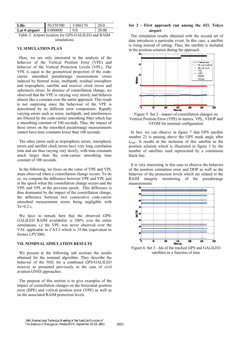
Figure 5: Set 2 - impact of constellation changes on Vertical Position Error (VPE) in meters, VPL, VDOP and

VFOM for nominal configuration

In fact, we can observe in figure 7 that GPS satellite number 23 is passing above the GPS mask angle after

. It results in the inclusion of this satellite in the position solution which is illustrated in figure 5 by the number of satellites used represented by a continuous black line.

It is very interesting in this case to observe the behavior of the position estimation error and DOP as well as the behavior of the protection levels which are related to the RAIM integrity monitoring of the pseudorange measurements.

Figure 6: Set 2 - Ids of the tracked GPS and GALILEO satellites as a function of time

3805

Figure 7: Set 2 - Elevation angle of GPS and GALILEO satellites as a function of time

In fact, we can see in figure 5 that the inclusion of a healthy satellite leads to a decrease of the VPL as well as a slight decrease of the VDOP. The same effect can be observed in the horizontal plane in figure 8: the inclusion of GPS satellite 23 leads to a decreasing step in the HPE as well as in the HDOP. The HPL does not seem to be really impacted. However, HPL were already very low since during the whole approach the receiver was tracking a minimum of 19 satellites. To conclude, we can see that, in this simulation, the impact of the inclusion of a new satellite can be considered as negligible due to the high number of satellites already available, thanks to the tracking of two different GNSS constellations.

Figure 8: Set 2 - impact of constellation change on Horizontal Position Error (HPE) in meters, HPL, HDOP

and HFOM for nominal configuration

Our approach for the statistical analysis of the simulations was to first evaluate the impact of constellation changes on the position estimation error during the whole approach and then to distinguish the constellation changes occurring during the beginning of the approach (before the FAF) and the ones occurring during the final approach (after the FAF).

Results over the complete approach

First, we updated a single histogram with each observed value of Vertical Position Error during all simulations, that is to say for all simulated approaches and for all airports, which is illustrated in figure 9.

Figure 9: Histogram of estimated VPE over all simulations for the complete approaches in nominal

configuration

As we can see, we clearly obtained a mono modal Gaussian shaped histogram. What is interesting is that, thanks to this figure, we were able to compute the global standard deviation of the VPE during our simulations which is around 1.023 meters. Applicable regulations for CAT-I operations require an accuracy lower than 4 meters at least 95% of the time. We know that for Gaussian variables, the CDF reaches the probability of 95% at around 2 times the standard deviation. With our observed results we thus obtain 2 x 1.023 which gives 2.046 meters, which is far lower than 4 meters. We can conclude here that the studied position solution can fulfil the accuracy requirements of CAT I precision approaches.

Then, we have represented in figure 10 the histogram of the estimated average value of the vertical position estimation error. Each average value used to build this histogram was derived using the samples of one simulation run, it was thus obtained by averaging

samples. Thus, the histogram is finally composed of mean values. As we can see, the obtained distribution has a mono-modal Gaussian shape. The minimum and maximum values of the estimated average vertical position errors over the approach are respectively and .

Figure 10: Histogram of the estimated mean of VPE over all simulation runs for the complete approaches in

nominal configuration

-6 -4 -2 0 2 4 60

0.005

0.01

0.015

0.02

0.025

METERS

PE

RC

EN

TAG

E

APPCH: VPE VARIATIONS (min=-4.9 m, max=4.9 m)

-6 -4 -2 0 2 4 60

0.005

0.01

0.015

0.02

0.025

METERS

PE

RC

EN

TAG

E

HISTOGRAM OF ESTIMATED MEAN OF VERTICAL POSITION ERROR

APPCH: MEAN VERT (min=-4.39 m, max=4.19 m)

3806

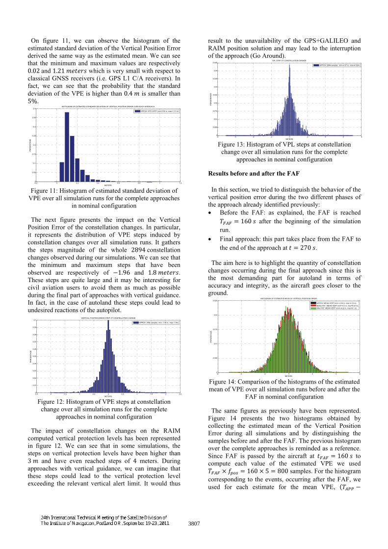
On figure 11, we can observe the histogram of the estimated standard deviation of the Vertical Position Error derived the same way as the estimated mean. We can see that the minimum and maximum values are respectively

and which is very small with respect to classical GNSS receivers (i.e. GPS L1 C/A receivers). In fact, we can see that the probability that the standard deviation of the VPE is higher than is smaller than

.

Figure 11: Histogram of estimated standard deviation of VPE over all simulation runs for the complete approaches

in nominal configuration

The next figure presents the impact on the Vertical Position Error of the constellation changes. In particular, it represents the distribution of VPE steps induced by constellation changes over all simulation runs. It gathers the steps magnitude of the whole constellation changes observed during our simulations. We can see that the minimum and maximum steps that have been observed are respectively of and .These steps are quite large and it may be interesting for civil aviation users to avoid them as much as possible during the final part of approaches with vertical guidance. In fact, in the case of autoland these steps could lead to undesired reactions of the autopilot.

Figure 12: Histogram of VPE steps at constellation change over all simulation runs for the complete

approaches in nominal configuration

The impact of constellation changes on the RAIM computed vertical protection levels has been represented in figure 12. We can see that in some simulations, the steps on vertical protection levels have been higher than

and have even reached steps of meters. During approaches with vertical guidance, we can imagine that these steps could lead to the vertical protection level exceeding the relevant vertical alert limit. It would thus

result to the unavailability of the GPS+GALILEO and RAIM position solution and may lead to the interruption of the approach (Go Around).

Figure 13: Histogram of VPL steps at constellation change over all simulation runs for the complete

approaches in nominal configuration

Results before and after the FAF

In this section, we tried to distinguish the behavior of the vertical position error during the two different phases of the approach already identified previously:

Before the FAF: as explained, the FAF is reached after the beginning of the simulation

run. Final approach: this part takes place from the FAF to the end of the approach at .

The aim here is to highlight the quantity of constellation changes occurring during the final approach since this is the most demanding part for autoland in terms of accuracy and integrity, as the aircraft goes closer to the ground.

Figure 14: Comparison of the histograms of the estimated mean of VPE over all simulation runs before and after the

FAF in nominal configuration

The same figures as previously have been represented. Figure 14 presents the two histograms obtained by collecting the estimated mean of the Vertical Position Error during all simulations and by distinguishing the samples before and after the FAF. The previous histogram over the complete approaches is reminded as a reference. Since FAF is passed by the aircraft at to compute each value of the estimated VPE we used

samples. For the histogram corresponding to the events, occurring after the FAF, we used for each estimate for the mean VPE,

-0.2 0 0.2 0.4 0.6 0.8 1 1.20

0.05

0.1

0.15

0.2

0.25

0.3

0.35

0.4

METERS

PE

RC

EN

TAG

E

HISTOGRAM OF ESTIMATED STANDARD DEVIATION OF VERTICAL POSITION ERROR OVER EACH APPROACH

APPCH: STD VERT (min=0.02 m, max=1.21 m)

-2.5 -2 -1.5 -1 -0.5 0 0.5 1 1.5 2 2.50

0.01

0.02

0.03

0.04

0.05

0.06

0.07

0.08

0.09

0.1VERTICAL POSITION ERROR STEP AT CONSTELLATION CHANGE

METERS

PE

RC

EN

TAG

E

APPCH: 2894 samples, min=-1.96 m, max=1.8m)

-8 -6 -4 -2 0 2 4 6 80

0.005

0.01

0.015

0.02

0.025

0.03

0.035

0.04

0.045VPL STEP AT CONSTELLATION CHANGE

METERS

PE

RC

EN

TAG

E


-6 -4 -2 0 2 4 60

0.005

0.01

0.015

0.02

0.025

METERS

PE

RC

EN

TAG

E


APPCH: MEAN VERT (min=-4.39 m, max=4.19 m)Before FAF: MEAN VERT (min=-4.5 m, max=4.24 m)After FAF: MEAN VERT (min=-4.22 m, max=4.1 m)

3807

samples. As previously done, we thus obtained

estimated mean VPE to build each histogram.

Minimumestimatedmean VPE

Maximumestimatedmean VPE

Completeapproach

4.39 4.19

Before FAF 4.5 4.24After FAF 4.22 4.1

Table 3: Minimum and maximum estimated mean VPE observed in nominal configuration

This figure shows that the different histograms obtained have Gaussian shapes. The maximum and minimum mean values observed which are gathered in the previous table are nearly the same which is quite logical since the position of the aircraft in the approach has a limited impact on the mean VPE. We can however see here that the maximum estimated mean values of the VPE are observed before the FAF with and

.

Figure 15: Comparison of the histograms of estimated standard deviation of VPE over all simulation runs before

and after the FAF in nominal configuration

On the contrary, the results are slightly different when we take a look at the estimated standard deviation of the VPE represented in figure 15. The minimum and maximum estimated standard deviations of VPE observed are gathered in the following table:

Minimumestimatedstd VPE

MaximumestimatedstdVPE

Completeapproach

0.02 1.21


Table 4: Minimum and maximum estimated VPE standard deviation observed in nominal configuration

In fact, we have already seen that if we make no distinction between the first part of the approach and the final approach, the maximum observed standard deviation of VPE was about and we also observed that the standard deviation was lower than more than 95 %

of the time. However, if we distinguish the standard deviation before and after the FAF, we can see that the obtained standard deviation histograms are different. On the one hand, before the FAF, the observed standard deviation has a higher maximum of about . On the other hand, after the FAF the observed standard deviation has a maximum value of about and the corresponding histogram is more concentrated in the lower VPE standard deviation magnitude. So, we can see that globally, the VPE standard deviation is lower during the Final approach than before the FAF.

Figure 16: Comparison of the histograms of VPE steps at constellation change over all simulation runs before and

after the FAF in nominal configuration

We then look at the distribution and the magnitude of the VPE steps due to a constellation change during the approach thanks to figure 16. A total number of

constellation changes have been detected during our simulations resulting in VPE steps of minimum and maximum amplitude which are gathered in the following table:

MinimumVPE steps

MaximumVPE steps

Completeapproach

1.96 1.8


Table 5: Minimum and maximum estimated VPE steps observed in nominal configuration

The most interesting result is that we have observed the same number of VPE steps caused by constellation changes before and after the FAF. In fact, we observed 1447 steps before the FAF and 1447 steps after the FAF. If we express the probability of occurrence of a step per approach we thus obtain:

As we can see, the probability that a constellation change occurs during the approach is quite high. In terms of magnitude, we can see that the distributions of the VPE steps magnitude have Gaussian shapes with the minimum and maximum observed values being around

and equivalently before and after the FAF.

-0.2 0 0.2 0.4 0.6 0.8 1 1.20

0.05

0.1

0.15

0.2

0.25

0.3

0.35

0.4

0.45

0.5

METERS

PE

RC

EN

TAG

E


APPCH: STD VERT (min=0.02 m, max=1.21 m)Before FAF: STD VERT (min=0.02 m, max=1.52 m)After FAF: STD VERT (min=0 m, max=0.91 m)

-2.5 -2 -1.5 -1 -0.5 0 0.5 1 1.5 2 2.50

0.02

0.04

0.06

0.08

0.1


METERSP

ER

CE

NTA

GE

APPCH: 2894 samples, min=-1.96 m, max=1.8m)Before FAF: 1447 samples, min=-1.92 m, max=1.77m)After FAF: 1447 samples, min=-1.96 m, max=1.8m)

3808

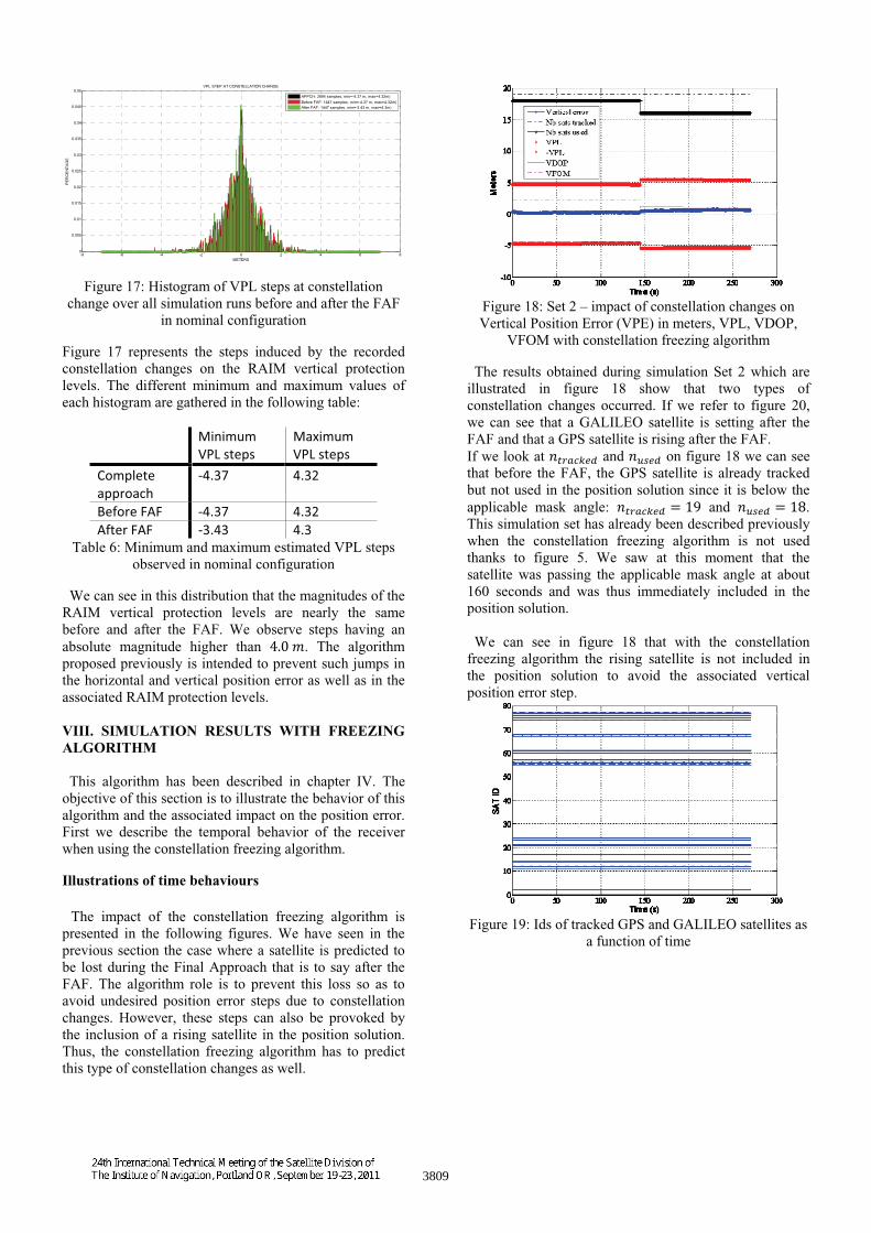
Figure 17: Histogram of VPL steps at constellation change over all simulation runs before and after the FAF

in nominal configuration

Figure 17 represents the steps induced by the recorded constellation changes on the RAIM vertical protection levels. The different minimum and maximum values of each histogram are gathered in the following table:

MinimumVPL steps

MaximumVPL steps

Completeapproach

4.37 4.32


Table 6: Minimum and maximum estimated VPL steps observed in nominal configuration

We can see in this distribution that the magnitudes of the RAIM vertical protection levels are nearly the same before and after the FAF. We observe steps having an absolute magnitude higher than . The algorithm proposed previously is intended to prevent such jumps in the horizontal and vertical position error as well as in the associated RAIM protection levels.

VIII. SIMULATION RESULTS WITH FREEZING ALGORITHM

This algorithm has been described in chapter IV. The objective of this section is to illustrate the behavior of this algorithm and the associated impact on the position error. First we describe the temporal behavior of the receiver when using the constellation freezing algorithm.

Illustrations of time behaviours

The impact of the constellation freezing algorithm is presented in the following figures. We have seen in the previous section the case where a satellite is predicted to be lost during the Final Approach that is to say after the FAF. The algorithm role is to prevent this loss so as to avoid undesired position error steps due to constellation changes. However, these steps can also be provoked by the inclusion of a rising satellite in the position solution. Thus, the constellation freezing algorithm has to predict this type of constellation changes as well.

Figure 18: Set 2 – impact of constellation changes on Vertical Position Error (VPE) in meters, VPL, VDOP,

VFOM with constellation freezing algorithm

The results obtained during simulation Set 2 which are illustrated in figure 18 show that two types of constellation changes occurred. If we refer to figure 20, we can see that a GALILEO satellite is setting after the FAF and that a GPS satellite is rising after the FAF. If we look at and on figure 18 we can see that before the FAF, the GPS satellite is already tracked but not used in the position solution since it is below the applicable mask angle: and .This simulation set has already been described previously when the constellation freezing algorithm is not used thanks to figure 5. We saw at this moment that the satellite was passing the applicable mask angle at about 160 seconds and was thus immediately included in the position solution.

We can see in figure 18 that with the constellation freezing algorithm the rising satellite is not included in the position solution to avoid the associated vertical position error step.

Figure 19: Ids of tracked GPS and GALILEO satellites as a function of time

-8 -6 -4 -2 0 2 4 6 80

0.005

0.01

0.015

0.02

0.025

0.03

0.035

0.04

0.045


METERS

PE

RC

EN

TAG

E

APPCH: 2894 samples, min=-4.37 m, max=4.32m)Before FAF: 1447 samples, min=-4.37 m, max=4.32m)After FAF: 1447 samples, min=-3.43 m, max=4.3m)

3809

Figure 20: Elevation angle of GPS and GALILEO satellites as a function of time

Moreover, we can see that a satellite is artificially removed from the position solution at the FAF since it is predicted as setting after the FAF and before the touchdown. This case is interesting since if we compare this result with figure 20, we can see that in fact the satellite is setting just after the touchdown of the aircraft and thus it could have been used during the approach. Thus, in this case, our algorithm has erroneously removed the satellite from the position solution due to the margins implemented and the simplicity of our prediction model (linear extrapolation). However, we can consider that since there are still satellites available, this error is not an issue.

VIII.2. Statistical results

Results over the complete approach

Figure 21 represents the collection of each observed VPE value for all simulation runs.

Figure 21: Histogram of estimated VPE over all simulations for the complete approaches with

constellation freezing algorithm What is interesting here is to compare the obtained results using the constellation freezing algorithm and the results presented in figure 9 without this algorithm. What we can see is that the maximum VPE has slightly increased with respect to the previous one since we observed here a maximum VPE value of 5.64 meters

while in the nominal case the maximum observed value of VPE was of 4.8 meters. However, if we compute the standard deviation of the VPE we obtained a value of 1.006 meters while we obtained 1.023 meters in the nominal case. Consequently, the constellation freezing algorithm led to a very small decrease of this standard deviation. If we combine these two results, we can in fact conclude that the position solution has not been degraded by the use of our algorithm even if we limit the number of tracked satellites. Moreover, we can remark that in both cases the position solution is easily verifying the accuracy requirements applicable to CAT-I precision approaches operations.

Figure 22 represents the histogram of the estimated mean of the vertical position error. As previously said, each average value has been computed using the output samples produced during one simulated approach and the histogram is thus composed of mean values. The obtained distribution has a mono-modal Gaussian shape. As we can see, the observed value of the estimated average vertical position error over the complete approach ranges in [-3.89 m, 3.54 m] which is slightly smaller than the values observed in the previous simulations and represented in figure 10.

Figure 22: Histogram of estimated mean of VPE over all simulation runs for the complete approaches

In fact, it is possible that by using the proposed algorithm to fix the satellite constellation after the FAF, we have improved the receiver positioning accuracy. The algorithm induces two different behaviours:

It can anticipate the loss of a satellite during final approach and force this loss to happen before sequencing the FAF. In this case, since the duration of the approaches are quite small we can imagine that the position error introduced due to the loss of a satellite is the same if it occurs naturally or if it is triggered by the algorithm. However, since the satellites are at low elevations, the associated errors such as ionosphere and troposphere may vary very rapidly, inducing significant residual errors differences before and after the FAF. It can anticipate the inclusion of a new satellite in the position solution and avoid it. In this case, we can imagine two different impacts. The inclusion of a new satellite could increase the accuracy of the

-6 -4 -2 0 2 4 60

0.005

0.01

0.015

0.02

0.025

METERS

PE

RC

EN

TAG

E


-6 -4 -2 0 2 4 60

0.005

0.01

0.015

0.02

0.025

METERS

PE

RC

EN

TAG

E


APPCH: MEAN VERT (min=-3.89 m, max=3.54 m)

3810

position solution due to the enhancement of the DOP for example. Thus, by forbidding this inclusion we may degrade the position solution. However, in our case the mean position error seems lower. It could be explained by the fact that due to the high number of available satellites, it could be more beneficial to not include the new satellites due to the trade-off between the improvements of the constellation geometry with respect to the additional measurement errors introduced by the new satellite. The results presented in figure 22, seems to indicate that the additional noise, multipath, ionosphere, troposphere uncertainties brought by the new satellite overcome the improvement of the constellation geometry.

Figure 23: Histogram of estimated std of VPE over all simulation runs for the complete approaches

Figure 23 shows the histogram of the estimated standard deviation of the vertical position error. The estimated standard deviation of the vertical position error over the 1350 samples of the complete approach ranges in [0.02 m; 1.38 m]. This histogram is nearly the same as the equivalent one for the initial simulations ran without the proposed constellation freezing algorithm and presented in figure 12. The standard deviation of the vertical position error thus does not seem to be impacted.

Figure 24: Histogram of VPE steps at constellation change over all simulation runs for the complete

approaches

Figure 24 shows the histogram of the vertical position error (VPE) steps occurring when constellation changes occur, as observed during the 270s approaches triggered at 433 time samples over the 16 airports. We can see that 2586 constellation changes are observed. The vertical position error steps due to constellation changes range in

[-2.05 m; 2.63 m]. This represents a small increase with respect to the results presented previously when the constellation freezing algorithm was not used since the maximum amplitude of vertical position error step was

as we can see in figure 13. However, note that infigure 24, the value of 2.63 m has only been observed once.

Figure 25: Histogram of VPL steps at constellation change over all simulation runs for the complete

approaches

The same pattern can be observed in figure 25 since the histogram of the observed steps of vertical protection levels induced by constellation changes illustrates that we observed steps ranging in while the steps recorded in figure 13 were ranging in .However, if we compare the results obtained with and without the constellation freezing algorithm, we can conclude that the different histograms have globally the same shapes and that the quantities recorded have nearly the same behaviour. Thus, we can consider that the algorithm has a minor impact on the size of the steps in vertical protection levels and vertical position error and we can assume that it has degraded our position solution in a negligible way because these larger VPL and VPE values are isolated outlier samples.

Figure 26: Histogram of VPE variations over all simulation runs for the complete approach

We were also interested in the behaviour of the NSE at the output of the combined GPS-GALILEO receiver. To do so, we extracted the VPE variations from the observed VPE by computing the difference of VPE between each consecutive epoch of simulation. The results obtained

-0.2 0 0.2 0.4 0.6 0.8 1 1.20

0.05

0.1

0.15

0.2

0.25

0.3

0.35

0.4

METERS

PE

RC

EN

TAG

E


APPCH: STD VERT (min=0.02 m, max=1.38 m)

-2.5 -2 -1.5 -1 -0.5 0 0.5 1 1.5 2 2.50

0.01

0.02

0.03

0.04

0.05

0.06

0.07

0.08

0.09


METERS

PE

RC

EN

TAG

E


-8 -6 -4 -2 0 2 4 6 80

0.005

0.01

0.015

0.02

0.025

0.03

0.035

0.04

0.045


METERS

PE

RC

EN

TAG

E


-6 -4 -2 0 2 4 60

0.005

0.01

0.015

0.02

0.025

METERS

PE

RC

EN

TAG

E


3811

were used to update a single histogram which can be seen in figure 26.

The following section insists on the comparison of the position error before and after the FAF.

Results before and after the FAF

The intent here is to characterize the vertical position error as well as the vertical protection levels before and after the FAF and to illustrate the impact of the proposed algorithm.

Figure 27: Comparison of the histograms of estimated mean of VPE over all simulation runs before and after the

FAF with constellation freezing algorithm

Figure 27 allows comparing the histogram of the estimated average vertical position error:

over the complete approach each mean value being computed using the

samples of a complete approach before the FAF, each mean value being computed using samples

after the FAF, each mean value being computed using samples

Since we did simulations over different airports each histogram is composed

of 6928 values of estimated mean. As previously said, each distribution has a mono-modal Gaussian shape. The different minimum and maximum values of each histogram are gathered in the following table:

Minimumestimatedmean VPE

Maximumestimatedmean VPE

Completeapproach

3.89 3.54


Table 7: Minimum and maximum estimated mean VPE observed with constellation freezing algorithm

If we compare these results with the results obtained for the nominal configuration of the receiver and represented in figure 13, we can see that we globally obtained lower mean VPE over the complete approach. No further

conclusion can be deduced from the overall shapes of these distributions. The interest here is to observe the potential impact of the proposed algorithm by comparing the mean VPE before and after the FAF. We can see that globally the different distributions have nearly the same Gaussian shapes with minimum and maximum which are really close to each other. Thus we can conclude that the algorithm has improved the mean vertical position solution error in a negligible way.

Figure 28: Comparison of histograms of estimated std of VPE over all simulation runs before and after the FAF

with constellation freezing algorithm

We can observe the associated histograms of the estimated standard deviation of the VPE in figure 28.The different minimum and maximum of these histograms are gathered in the following table:

Minimumestimatedstd VPE

Maximumestimatedstd VPE

Completeapproach

0.02 1.38

Before FAF 0.02 1.71After FAF 0 0.79

Table 8: Minimum and maximum estimated mean VPE observed with constellation freezing algorithm

What we can see is that the implementation of the constellation freezing algorithm resulted in a reduction of the estimated standard deviation of the vertical position error after the FAF to a maximum value of with our algorithm compared to a maximum value of without. The counterpart of course is that the standard deviation of the VPE before the FAF has varied accordingly by increasing to a value of .

To conclude, when using the proposed algorithm, all steps resulting from a constellation change are forced to happen before the aircraft sequences the FAF. No constellation change is occurring after the FAF and thus no VPE or VPL steps, resulting in the stabilization of the position error between the FAF and the touchdown.

IX. CONCLUSION

This paper presents the simulation results obtained with a GPS/GALILEO and RAIM simulator developed in the course of this study. The main objective of the

-6 -4 -2 0 2 4 60

0.005

0.01

0.015

0.02

0.025

METERS

PE

RC

EN

TAG

E


APPCH: MEAN VERT (min=-3.89 m, max=3.54 m)Before FAF: MEAN VERT (min=-4.06 m, max=3.58 m)After FAF: MEAN VERT (min=-3.83 m, max=3.98 m)

-0.2 0 0.2 0.4 0.6 0.8 1 1.20

0.1

0.2

0.3

0.4

0.5

0.6

0.7

METERS

PE

RC

EN

TAG

E


APPCH: STD VERT (min=0.02 m, max=1.38 m)Before FAF: STD VERT (min=0.02 m, max=1.71 m)After FAF: STD VERT (min=0 m, max=0.79 m)

3812

simulations was to observe the impact of constellation changes on the position error at the output of the simulated GPS/Galileo receiver. In fact, constellation changes can induce undesired steps in the NSE which could be lead to unwanted guidance errors during the final phase of a precision approach.

As we can see, thanks to the obtained results, the position error is quite small, mainly due to the high redundancy in terms of satellites brought by the combination of two different GNSS constellations. We have to remark that even if we did not run complete availability simulations, the RAIM protection levels have never exceeded the relevant alert limits. However, simulations have also proven that constellation changes still create unexpected position error steps.

To handle this phenomenon a simple algorithm has been developed to guarantee that there will not be error steps during the most critical part of the CAT I precision approaches which is considered to be defined between the FAF and the touchdown of the aircraft. To do so this algorithm makes a simple prediction of the constellation evolution by extrapolating the satellites position. It is thus capable to forecast which satellites will potentially rise or set during the final approach. The next step is to freeze the constellation at the FAF: • Satellites which are predicted as setting during final approach are automatically removed at the FAF • Satellites which are predicted to rise during final approach are automatically inhibited and are thus not included

This algorithm thus results in no position error steps during the final approach phase. We have also observed that there is a significant reduction of the maximum sigma of the VPE after the FAF as well as the global maximum mean VPE.

X. REFERENCES

[BETZ, 2000], J. W. Betz and K.R. Kolodziejski, “Extended Theory of Early-Late Code Tracking for Bandlimited GPS receiver”, Navigation: Journal of The Institute of Navigation, Fall 2000

[ESA, 2005], European Space Agency, “GALILEO Integrity Concept”, Technical Note, Jul. 2005

[EUROCAE, 2007], EUROCAE WG-62, “Interim Minimum Operational Performance Specification for Airborne GALILEO Satellite Receiving Equipment”, version 0.26, 2007

[GPS SPS, 2008], “Global Positioning System Standard Positioning Service Performance Standard”, Department of Defense, United States Of America, Sept. 2008

[HAHN, 2005], Hahn J. H., E.D. Powers, “Implementation of the GPS to GALILEO Time Offset

(GGTO)”, IEEE Frequency Control Symposium and Exposition, August 2005

[HEGARTY, 2006], C. Hegarty, “Analytical derivation of maximum tolerable in-band interference level for aviation applications of GNSS”, 1996

[HURST, 1972], Hurst R.L. and Knop R.E., “Generation of Random Correlated Normal Variables”, Communications of the ACM, Vol.15, No5, 1972

[JULIEN, 2005], Olivier JULIEN, “Design of GALILEO L1F Receiver Tracking Loops”, PhD Thesis, University Of Calgary, Jul. 2005

[MACABIAU, 2006], C.Macabiau, M. Moriella, M.Raimondi, C.Dupouy, A. Steingass, A. Lehner, “GNSS Airborne Multipath Errors Distribution Using the High Resolution Aeronautical Channel Model and Comparison to SARPS Error Curve”, Proceedings of ION NTM 2006

[MARTINEAU, 2008], Martineau A., “Perfomance of Receiver Autonomous Integrity Monitoring (RAIM) for Vertically Guided Approaches”, PhD thesis, Institut National Polytechnique de Toulouse, Nov. 2008

[RTCA, 2006], “Minimum Operational Performance Standards for Global Positioning System/Wide Area Augmentation System Airborne Equipment”, DO229-D, RTCA SC-159, 2006

[SALOS, 2010], S.Salos, C.Macabiau, A.Martineau, B.Bonhoure, D.Kubrak, “Nominal GNSS pseudorange measurement model for vehicular urban application”, Proceedings of IEEE/ION PLANS 2010

[SPILKER, 1996], J.SPILKER, Global Positioning System: Theory and Application, volume1, AIAA, 1996

[STEINGASS, 2004], A.Steingass, A.Lehner, F.Pérez Fontán, E.Kubista, M.Jesús Martin and B.Arbesser-Rastburg, “The High Resolution Aeronautical Multipath Navigation Channel”, Proceedings of ION GPS 2004

[STEPHENS, 1995], S.A. Stephens, J.B. Thomas, “Controlled-Root Formulations for Digital Phase Locked Loops”, IEEE Transactions on Aerospace and Electronic Systems, Vol.31, 1995

3813

study of the temporal behavior of gps/galileo nse...

Documents