study of marine gas hydrate on the northern cascadia ...€¦ · study of marine gas hydrate on the...
TRANSCRIPT
Study of Marine Gas Hydrate on the Northern
Cascadia Margin: Constraints from Logging and
Seismic Interpretation
Xuan Wang
Department of Earth and Planetary Sciences
McGill University, Montreal
Submitted:
April 09, 2009
A thesis submitted to McGill University in partial fulfillment of the
requirements of the degree of Master of Science
© Xuan Wang 2009

i
ABSTRACT
This thesis presents estimates of gas hydrate distribution and saturation
utilizing data from the four IODP Expedition 311 drilling sites, located at the
northern Cascadia Margin. The objectives are to constrain geologic models of
hydrate formation by determining mechanisms controlling magnitude and
distribution of hydrate occurrences, finding pathways enabling fluid
migration, and examining the effect of hydrate on physical properties of the
sediment. Well log and core data are used to calculate hydrate concentrations,
complemented by pore-fluid geochemical data. Correlation of seismic and
logging data is achieved through synthetic seismograms. Lithology and
faulting appears to control hydrate occurrences, which contradicts established
hydrate formation models. Individual sedimentary layers (e.g. turbidites) and
abundant faults act as migration pathways for fluids and gas explaining the
high hydrate concentrations at shallow depths of less than 100 meters below
seafloor, instead of the previously predicted enrichment near the base of the
hydrate stability zone.

ii
ABSTRAIT
Cette thèse présente des estimations de la distribution et de la
saturation des hydrates de gaz, en utilisant des données provenant des quatres
sites des forages océaniques effectués durant l’expédition 311 de l’IODP,
situés au nord de la marge de Cascadia. Les objectifs de cette étude sont
d’établir des modèles géologiques d’hydrates de gaz en déterminant les
mécanismes contrôlant leurs ampleurs et leurs distributions, les voies
permettant la migration de fluides, en plus d’examiner l’effet des hydrates
sur les propriétés physiques de sédiment. Les concentrations d’hydrates sont
calculées à partir des données provenant de techniques de diagraphie et de
carottage, complétées par des données géochimiques. La calibration de
données sismiques est faite à l’aide d’informations issues des diagraphies de
puits, générant des sismogrammes synthétiques. Les failles et la lithologie
contrôlent l’occurrence des hydrates, contredisant certains modèles
géologiques déjà établies. Les couches individuelles de sédiments (e.g.
turbidites) et l’abondance de failles deviennent des voies de migration pour
l’accumulation de fluides et de gaz. Ceci expliquerait les hautes
concentrations d’hydrates présent à 100 mètres en-dessous du fond de la mer,
et non comme un enrichissement, prédis précédemment près de la base de la
zone de stabilité des hydrates.

iii
ACKNOWLEDGEMENTS
First of all, I wish to give my earnest thanks to my supervisor Michael
Riedel who has provided me with a most inspiring research environment and
has guided me with the utmost patience by his rich knowledge and
experiences, invaluable suggestions and firm support. Thanks for his valuable
suggestions and all the effort he put into my thesis, I cannot have this
achievement without his help.
I would also like to thank several individuals for assistance and warmly
encouragement during my thesis. Many thanks for my boyfriend Zhongwei
Wang who provided invaluable suggestions on programming and data editing.
Thanks also to Jonathan Menivier, who helped me to translate the abstract into
French. Thanks for Peter Neelands who provided high resolution bathymetry
data for this thesis.
I would like to express my gratitude to all the faculty members in the
Department of Earth & Planetary Sciences, who have helped me firmly
through various hard times.
Thanks to all of my friends, thank you for making my life in Montreal
colorful and memorable.
Finally, thanks for my parents, Qing Wang and Yuerong Sue, I owe all
my success to you.

iv
LIST of ABBREVIATIONS
AI Acoustic Impedance
APC Advanced Piston Corer APCT Piston Corer Temperature AVO Amplitude-Versus-Offset
BGHSZ Base of Gas Hydrate Stability Zone BSR Bottom Simulating Reflector CDPs Common Depth Points
CORKs Instrumented Borehole Seals DIT Dual Induction Tool
DSDP Deep Sea Drilling Project DSI Dipole Sonic Imager
DTAGS Deep-Tow Acoustics Geophysics System DVTP Davis-Villinger Temperature Probe
DVTPP Davis-Villinger Temperature-Pressure Probe GHOZ Gas Hydrate Occurrence Zone HNGS Hostile Environment Gamma Ray Sonde IODP Integrated Ocean Drilling Program LWD Logging while Drilling MAD Moisture and Density mbsl meters below sea floor MCS Multi-Channel Seismic MWD Measurement while drilling
NEPTUNE Northeast Pacific Time-Series Undersea Networked Experiment OBS Ocean Bottom Seismographs ODP Ocean Drilling Program RC Refelection Coefficient
ROPOS Remotely Operated Platform for Ocean Sciences SGT Scintillation Gamma Ray Tool TAP Temperature/ Acceleration/ Pressure TWT Two-Way-Traveltime VSP Vertical Seismic Profile XCB Extended Core Barrel

v
TABLE of CONTENTS
CHAPTER 1 INTRODUCTION.............................................................................................1 1.1 OVERVIEW AND OBJECTIVES OF THE STUDY.....................................................................1 1.2 INTRODUCTION TO STUDY AREA .......................................................................................2 1.3 GAS HYDRATE DEFINITION, OCCURRENCE AND DISTRIBUTION .........................................3
1.3.1 Significance of gas hydrate: Potential future fuel resource.....................................4 1.3.2 Significance of gas hydrate: Implication in geohazard issues .................................5 1.3.3 Significance of gas hydrate: A source of green-house gas?.....................................6
1.4 POSSIBLE GAS HYDRATE FORMATION SCENARIOS .............................................................6 CHAPTER 2 OVERVIEW OF PREVIOUS GAS HYDRATE STUDIES OFFSHORE VANCOUVER ISLAND..........................................................................................................9
2.1 SUMMARY OF PREVIOUS SEISMIC WORK AND GAS HYDRATE CONCENTRATION ESTIMATES...............................................................................................................................................9 2.2 SUMMARY OF ODP LEG 146 WORK AND ACHIEVEMENTS ...............................................14 2.3 SUMMARY OF IODP EXPEDITION 311.............................................................................15
2.3.1 Introduction ...........................................................................................................15 2.3.2 Site descriptions.....................................................................................................16
2.4 LOG DATA INTERPRETATION FOR GAS HYDRATE ASSESSMENT........................................17 CHAPTER 3 GAS HYDRATE SATURATION FROM WELL LOGGING CONSTRAINTS .....................................................................................................................19
3.1. GAS HYDRATE OCCURRENCES IN NATURE AND LOGGING APPROACHES.........................19 3.2 ELECTRICAL RESISTIVITY MEASUREMENTS AND ARCHIE’S LAW.....................................20
3.2.1 Archie’s law ...........................................................................................................20 3.2.2 Determing the empirical parameters .....................................................................22 3.2.3 Bulk Density-porosity calculation..........................................................................24 3.2.4 Log resistivity.........................................................................................................24
3.3 ARCHIE ANALYSES ESTIMATES FOR THE IODP EXPEDITION 311 TRANSECT DRILL SITES 25 3.3.1 Site U1325..............................................................................................................25 3.3.2 Site U 1326.............................................................................................................28 3.3.3 Site U1327..............................................................................................................29 3.3.4 Site U1329..............................................................................................................30
3.4 GAS HYDRATE AMOUNT ESTIMATED FROM ACOUSTIC TRANSIT TIME LOGS.....................31 3.4.1 Introduction ...........................................................................................................31 3.4.2 Principle of using acoustic logs to estimate gas hydrate saturation......................35 3.4.3 Methodologies........................................................................................................36 3.4.4 Determining the Empirical weighting factor W .....................................................38 3.4.5 Determining the Gas hydrate saturation................................................................39
3.5 VELOCITY ANALYSES ESTIMATES FOR THE IODP EXPEDITION 311 TRANSECT DRILL SITES.............................................................................................................................................40
3.5.1 U1325 ....................................................................................................................40 3.5.2 U1326 ....................................................................................................................41 3.5.3 U1327 ....................................................................................................................41 3.5.4 U1329 ....................................................................................................................42
CHAPTER 4 REGIONAL SEISMIC ANALYSES AND SYNTHETIC SEISMOGRAMS..................................................................................................................................................43
4.1 SITE U1325.....................................................................................................................44 4.1.1 General Seismic description ..................................................................................44 4.1.2 Lithostratigraphy at Site U1325 ............................................................................48 4.1.3 Synthetic Seismogram generation and Log-to-seismic correlation........................49
4.2 SITE U1326.....................................................................................................................52 4.2.1 General description ...............................................................................................52 4.2.2 Lithostratigraphy at U1326 ...................................................................................55 4.2.3 Synthetic Seismogram generation and Log-to-seismic correlation........................56
4.3 SITE U1327....................................................................................................................57 4.3.1 General Description...............................................................................................57

vi
4.3.2 Lithostratigraphy at U1327 ...................................................................................60 4.3.3 Synthetic seismogram generation and Log-to-seismic correlation ........................61
4.4 SITE U1329.....................................................................................................................64 4.4.1 General description ...............................................................................................64 4.4.2 Lithostratigraphy at U1329 ...................................................................................65 4.4.3 Synthetic seismogram generation and Log-to-seismic correlation ........................66
CHAPTER 5 SUMMARY, UNCERTAINTIES, AND CONCLUSIONS..........................68 5.1 COMPARISON OF RESULTS: RESISTIVITY, VELOCITY AND SYNTHETIC SEISMOGRAM......68
5.1.1 Gas Hydrate Saturation Estimates.........................................................................68 5.1.2 Comparison with previous interpretation ..............................................................69
5.2 UNCERTAINTIES..............................................................................................................70 5.3 CONCLUSION ..................................................................................................................72
REFERENCES:......................................................................................................................74 FIGURES ................................................................................................................................85
TABLES ................................................................................................................................183 APPENDIX Ι : PROGRAMMING OF GAS HYDRATE SATURATION ESTIMATES FROM VELOCITY DATA .................................................................................................194

1
Chapter 1 Introduction
1.1 Overview and Objectives of the study
In this thesis, the main objectives are to characterize marine gas hydrate
occurrences and distribution along a margin-wide transect of drilling sites
located on the Northern Cascadia Margin, offshore Vancouver Island, Canada
by utilizing downhole well logging and seismic data, including Multi-channel
seismic (MCS), Single-Channel seismic (SCS) and Vertical Seismic Profile
(VSP) data.
The drilling data used in this thesis mainly come from Integrated Ocean
Drilling Program (IODP) Expedition 311 (Riedel et al., 2006a), which was
carried out during September – October 2005, and an additional cruise carried
out in August 2008. A transect of four deep drilling sites (U1325, U1326,
U1327, and U1329), which represent different stages in the evolution of gas
hydrate across the entire margin, was chosen during IODP Expedition 311 to
study the occurrences and formation of gas hydrate in accretionary complexes.
IODP Expedition 311 provides new data to the many previous gas hydrate
studies conducted on the Cascadia margin especially Ocean Drilling Program
(ODP) Legs 146 and 204, by extending the aperture of the transect sampled
and by introducing new tools to systematically quantify the gas hydrate
content of the sediments. It was the first part of a multi-expedition study of the
gas hydrate formation system on the northern Cascadia accretionary complex.
Further borehole monitoring experiments tied to the NEPTUNE (Northeast
Pacific Time-Series Undersea Networked Experiment) Canada cable
observatory, would complement these data. Geophysical well log data,
including Logging While Drilling (LWD), measurement while drilling
(MWD), and additional wire-line (WL) logs were carried out along each site
of the transect.
In this thesis, the LWD electrical resistivity and velocity data, wire-line
and MCS velocity data are analyzed combined with other log and core sample
data to calculate gas hydrate concentrations. Correlation of seismic data and
2
logging data is then achieved by generating synthetic seismograms to define
the detailed gas hydrate occurrence at each of the four transect drilling sites.
Results from the geophysical analyses are complemented by geochemical pore
fluid data to further constrain gas hydrate formation characteristics. A more
recent cruise was carried out at the Northern Cascadia Margin during August,
2008. Further seismic and core data were collected and analyzed with a range
of geophysical, geochemical and sedimentological techniques by the scientific
party of 2008-007-PGC Cruise to determine the role of natural gas hydrate in
the mechanics of slope collapse and the mechanism of natural gas movement
around the cold vent area. The data from this new expedition yield a better
understanding of the geologic controls, the evolution, and provide new insight
into the role of gas hydrate in slope stability.
A two-dimensional (2D) MCS line, acquired in 1989 prior to ODP Leg
146 connects all of the four drilling sites, providing a complementary measure
of seismic velocity at each drilling site and adjacent areas. The VSP data from
Hole U1327E are utilized to estimate the depth of the bottom simulating
reflector (BSR), which is usually considered as the interface between gas
hydrate (above BSR) and free gas (below the BSR). Chlorinity data from core
samples provided an independent estimate of gas hydrate concentration where
samples of fresher chlorinity values than the assumed background trend
indicate the presence of dissociated gas hydrate in the recovered core.
1.2 Introduction to study area
The Northern Cascadia margin is part of the Cascadia subduction zone,
which is a convergent plate boundary that stretches from northern Vancouver
Island to northern California. The deformation front separates the Juan de
Fuca, Explorer, and the Northern American Plate. The Oceanic crust subducts
beneath the continent at a rate of ~40mm/yr (Hyndman et al. 2001). The study
area of IODP Expedition 311 is located on the continental slope off Vancouver
Island. Four sites transect southwest-northeast across the margin (Fig. 1.1).
The young Juan de Fuca plate (6-8Ma) is continuously subducted beneath the
North American plate with the consequence that the sediments/rocks all along
the edges of the incoming oceanic plate are compressed (squeezed) and

3
uplifted. The incoming pre-Pleistocene hemipelagic sediments, which are
overlain by ~2-3km thick rapidly deposited Pleistocene turbidite sediments,
are scraped off the oceanic plate during the subduction at the deformation
front, and are accreted so that a large clastic sedimentary prism has formed
since the Eocene. Since the young hot oceanic plate has a relatively low
density and the incoming sediment section is thick, a very shallow trench with
a depth of only ~2500m has been formed at the deformation front. The first
elongated anticline ridge (where Site U1326 located) of the accretionary
wedge is then ~700 m higher compared to the adjacent basins further inland
from the deformation front. The nearest adjacent basin relative to the first
anticlinal ridge developed to the east and is covered by thick (~350m at least),
course-grained sand layers within clay-rich interlayers. The characters of the
sediment within this slope basin indicate that the sediments were transported
parallel to the uplifted bounding ridges (Riedel et al, 2006; Westbrook et al.,
1994).
1.3 Gas Hydrate definition, occurrence and
distribution
Gas hydrates are ice-like solids, which combine water molecules with one
or more hydrocarbon or-non-hydrocarbon gas molecules. The gas molecules
are trapped inside “cages” of hydrogen bonded water. Gas hydrate can only
form under suitable high pressure and low temperature conditions, which
defines the gas hydrate stability zone (Fig.1.3). Thus, natural gas hydrate can
only be found in permafrost regions or within sediments of the deep ocean
(Fig 1.4).
Due to its distinct geophysical and geochemical characteristics, the
presence of gas hydrate within sediments can be identified with well-logging,
seismic (and other remote-sensing geophysical techniques such as controlled-
source electromagnetic surveying) and core-geochemistry data. For example,
gas hydrates can substantially increase sediment electrical resistivity and
seismic velocity; the occurrence of BSRs in seismic profiles, which is usually
considered as the base of gas hydrate stability zone, confine the depth range

4
within which gas hydrates could appear (Hyndman, 1992). BSRs are observed
in reflection seismic data from continental margin worldwide, especially in
subduction zone accretionary prisms. In addition, gas hydrate can also be
indicated from local chlorinity data of recovered core samples. When gas
hydrate dissociates in sediments, it releases the gas and fresh water, with the
fresh water diluting the in situ pore fluid salinity (and chlorinity), thus
resulting in the fresher chlorinity values.
1.3.1 Significance of gas hydrate: Potential future fuel
resource
A widely quoted estimate of global methane gas in gas hydrate published
by the U.S. Geological Survey (Kvenvolden, 1993) predicts that there is twice
as much organic carbon in gas hydrate than in all recoverable and
unrecoverable conventional fossil fuel resources, including natural gas, coal
and oil, combined. Much of this large reservoir of carbon has been thought to
be located on continental slopes in close proximity to major energy-consuming
nations (Fig.1.4) However, the amount of hydrate-bound gas has been
repeatedly quantitatively estimated over the years (Fig. 1.5), though large
uncertainties remain (Milkov, 2004; Klauda et al., 2005).
Arctic gas hydrate reservoirs are potentially the first economically
exploitable reservoirs for the generation of natural gas from hydrate. Some
important arctic hydrate accumulations (Collett et al., 2008) have high
porosity and gas hydrate concentrations, within high intrinsic permeability
sand layers. Such parameters can be considered as the perfect condition for gas
hydrate production.
Compared to permafrost gas hydrate production, marine gas hydrates
have not been considered to represent a recoverable reservoir, and the
complexity of the production techniques is even more enhanced in the marine
environment because of the unconsolidated nature of the host sediments.
Originally estimation of marine gas hydrate reservoir is ~10,000 times larger
than the global conventional gas endowment. However, recent estimation is
5
smaller, although large uncertainties exist (Milkov A.V., 2004). Fig.1.5
compares historic and current estimates of total hydrate bound gas to proved
reserves of conventional gas.
1.3.2 Significance of gas hydrate: Implication in
geohazard issues
Due to the properties of gas hydrate, it can cause natural geohazards.
The decomposition of gas hydrate is speculated to generate a weakness in
continental margin sediments that may help explain some of the observed
patterns of continental margin slope instability. The processes of gas hydrate
formation expel the in situ pore water and take place of the porosity inside the
sediment. Both the growth and decomposition processes inside the sediments
may deteriorate the structure and strength of the sediments. If gas hydrates is
present over a large surface area, the weakened sediments may form potential
planes of weakness, and the potential for sediment failure and slope collapse is
increased. While the relationship between slope failures and gas hydrate
decomposition has not yet been proven, a number of empirical observations
support their potential connection (Paull, 2003). If correct, gas hydrate in near
seafloor sediments may play a significant role as a geohazard, especially in
earthquake-prone areas such as subduction zones.
In addition, new concerns about gas hydrate production emerge. For
example, ocean-based oil-drilling operations sometimes intersect methane
hydrate reservoirs above the oil deposits. As a drill penetrate through the
hydrate layers, the process can cause the hydrate to dissociate, the free gas
may explode, causing the drilling crew to lose control of the well. Another
concern is that unstable hydrate layers could give way beneath oil platforms or,
on a larger scale, even cause tsunamis. When gas hydrate layers are detected
above the reservoir of interest, the production process may require expensive
deviated wells to circumvent the gas hydrate occurrence.

6
1.3.3 Significance of gas hydrate: A source of green‐
house gas?
Although highly disputed, marine gas hydrate is a possible source for
green-house gases, not only because of the globally enormous inventory of gas
hydrate deposits, but also because the stability of gas hydrate deposits can
easily be disturbed by climate changes. Furthermore, dissociated gas hydrate
releases the free gas, which can move through the seabed and reach into the
ocean and/ or atmosphere. Fig. 1.6 shows the snapshot of a gas plume on the
mid-slope (near Site U1327) on Cascadia margin which was recorded by 18Hz
echo-sounders during the 2008-007-PGC Cruise. Several active gas plumes
have been observed on during and prior to the 2008 cruise. Although current
theories of how natural gas can penetrate the gas hydrate stability zone and
exit at the seabed through deep-water gas vents are un-tested, the plumes are
strong evidences to prove that the transportation of methane from deeper
geologic reservoirs to the oceanic and/or atmospheric systems can be quite
effective.
Gas-hydrate-bound methane contained in the sediments may also be
released by large-scale slumping adding methane to the atmosphere. The
speculated mechanism is to transport methane directly into the atmosphere
while bypassing processes, such as methane oxidation and dissolving in the
ocean. During the recent 2008-007-PGC Cruise, large slumps with significant
volumes of solid gas hydrates underneath, were investigated. Additionally,
sites with active release of free gas (indicated as gas plumes on acoustic
profiler data) were studied.
1.4 Possible gas hydrate formation scenarios
At the Northern Cascadia margin, the accretionary sedimentary prism has
been considered the most common host environment for marine gas hydrate
accumulation. In the past few decades, various observations, theories and
models have been brought forward to explain the origin and mechanism of the
free gas and the formation, distribution and stability of gas hydrate, and the
7
impact of the gas hydrate to surrounding host sediment (see Chapter 2 for a
review of the most important studies and findings). Gas hydrate forms if the
concentration of methane exceeds the critical concentration close to the local
solubility threshold. Hydrate will dissolve when the methane saturation falls
below the critical concentration. Gas hydrate formation is also controlled by
the characteristic of the host sediment (e.g. porosity, permeability) the rate of
sedimentation at the local area, the quantity and quality of the organic material,
and the vigor of biological productivity (Matthew et al. 2001). Other factors
like the concentration of gases other than methane, the salinity of the pore
water and the composition of the host sediment also play an important role in
gas hydrate stability zone (e.g. Clennell et al., 1999).
The BSR is believed to correspond to the deepest level at which methane
hydrate is stable; that means below the BSRs, methane may be present as
dissolved or free gas, but not as hydrate. The appearance of BSRs in seismic
sections may largely depend on whether there is sufficient upward pore fluid
expulsion through a thick clastic sedimentary sequence on accretionary
sedimentary prisms (Hyndman and Davis, 1992). The (mainly) biogenic
methane forms far deeper below the base of gas hydrate stability zone, which
is carried upwards by the expulsive fluid flow. When the methane-rich but not
necessarily saturated fluids pass into the gas hydrate stability zone, methane is
removed from the fluid to form the gas hydrate and the hydrate zone begins to
build upward (Fig.1.7). The model explained the origin of the large amounts of
methane and the lack of large quantity of free gas below the stability field.
However, most observations from IODP Expedition 311 contradict this model
in that the highest concentrations of gas hydrate do not necessarily occur
around the BSR.
From combined observations of IODP Expedition 311, gas hydrates are
present at different depths within the sediment and can be found significantly
above the BSR (especially at Site U1326 and U1327). The base of the local
gas hydrate occurrence can be shallower than the base of the
thermodynamically defined stability zone.
According to the model by Xu and Ruppel (1999), the base of gas hydrate
stability may also not coincide with the depth of the BSR. Methane gas
8
hydrate can also occur within this model in a meta-stable form below the base
of hydrate stability zone (and BSR).
An alternate free-gas model has been brought forward by Minshull et al.
(1994). The preferential development of the BSR in structures that would tend
to intercept fluid flow or migrating gas and the presence of free gas beneath
the BSR indicate a mechanism of BSR formation in which free methane gas
bubbles migrate upward into the hydrate stability field or is carried there in
advecting pore water. The gas hydrate zone will form downwards as more gas
migrates upward. However, this model still needs to be verified because gas in
vapor phase is thermodynamically strongly unstable in the hydrate stability
zone (e.g. Buffett, 2000).
The composition of the gas sources, which contribute to gas hydrate
formation, can be classified into two categories: microbial gas, which is
dominated by methane with 13Cδ signatures ranging from -90‰ to -60‰, and
thermogenic gas that contains higher concentrations of 2C + hydrocarbons and
methane with 13Cδ signatures range from -50‰ to -30‰ (Whiticar, 1999). It
is regarded that the majority of gas hydrate near the Earth’s surface is mainly
the result of biogenic conversion of organic matter into methane gas
(Hyndman et al, 1992). However, under certain circumstance, preferential
consumption of 122CO during 2CO reduction has been shown to enrich, or
fractionate, 132CO to the residual 2CO pool to the extent that methane
generated via this process acquires a 13Cδ signature that might be mistaken as
a mix or pure thermogenic source (Claypool et al., 1985; Kvenvolden and
Kastner, 1990; Whiticar et al., 1995).
Paull et al. (1994) postulated a third model of hydrate formation, where it
is produced from in situ local organic carbon. Microbial methane production
takes place below the depth of sulfate reduction. When methane saturates in
the sediment, additional methane production will from either gas hydrate or
free gas, which depends on local temperature and pressure conditions.
However, this model may have some limitations in explaining larger observed
gas hydrate accumulations at the Cascadia Margin, which may require a larger
influx of methane into the stability zone for hydrate formation since the
sediment only contains 0.5% organic carbon.

9
Chapter 2 Overview of Previous Gas
Hydrate Studies Offshore Vancouver
Island
Extensive geophysical studies have been carried out since 1985 to
constraint the occurrence, distribution, and concentration of gas hydrate and
underlying free gas on the Northern Cascadia margin, off Vancouver Island.
This chapter will present an overview of the previous studies and major results,
and linkages to the existing seismic data for more detailed interpretation and
regional extrapolation of gas hydrate occurrences will also be discussed.
2.1 Summary of Previous Seismic work and gas
hydrate concentration estimates
Natural occurrences of gas hydrates have been reported in the
geosciences literature since the early 1970s (e.g. Trofimuk et al., 1973, 1977;
Shipley et al., 1979). In 1985 a BSR was identified in seismic data and the
presence of gas hydrate was inferred on that basis on the margin off
Vancouver Island (Davis and Hyndman, 1989). A wide variety of geophysical
surveys have been carried out to investigate the characters of the gas hydrate
and underlying free gas on Northern Cascadia margin (Fig. 2.1).
The different seismic surveys and data-types include:
(1) Conventional multichannel seismic (MCS) survey lines, which have
been presented and discussed by Spence et al. (1991a, b). The seismic lines
were shot by Digicon Geophysical Corporation in 1989. The survey was
collected using a DSS-240 recording system. The airgun array source was a
tuned array with a total volume of 125L (7820 3in ). Shots were recorded by a
3600m streamer with 144 hydrophones, towed 183m behind the vessel. The

10
MCS survey provided amplitude data as a function of source-receiver offset,
which can be utilized in quantitative AVO analysis (e.g. Yuan et al., 1996,
1999; Chen, 2006);
(2) A pseudo 3-D high resolution MCS survey in the area of ODP Leg
146. The location of this 3-D seismic experiment (shot in 1999) was chosen in
the vicinity of the ODP Sites 889 and 890, which are located at the mid-slope
plateau. The survey location is between two topographic highs and also
covers the blank zones area. The survey was conducted in a NW-SE direction
with a single 40 in3 airgun and a 1.2 km long streamer (details see Riedel,
2001).
(3) Two single-channel seismic (SCS) surveys across known cold vents,
seismically characterized by strong amplitude reduction (thus the name ‘blank
zone”. The first survey carried out in 1999 showed prominent linear features in
seismic amplitude time-slices created from interference-patterns at the edges
of the cold vents (Riedel et al., 2002). The SCS survey carried out in 2000 was
located at the SE corner of the 1999 SC seismic survey, with NE-SW direction,
focusing on Bullseye Vent only (Fig. 2.2).
(4) A very high resolution Deep-Tow Acoustics Geophysics System
(DTAGS) multichannel system that is towed near the seafloor. This survey
was deployed in the area of investigation around the ODP Site in 1997
(Chapman et al., 2002). The system consists of a Helmholtz transducer source
emitting a chirp-like sweep signal of frequencies from 250-650 Hz and a 600m
long hydrophone streamer with two subarrays each containing 24 hydrophone
groups (Gettrust and Ross 1990: Gettrust et al., 1999; Chapman et al. 2002).
(5) Detailed regional SCS and MCS reflection mapping with several
different frequencies (Fink and Spence, 1999; Mi, 1996; Ganguly et al., 2000).
(6) Seismic surveys using Ocean Bottom Seismometers (OBS) for 2-D
and 3-D inversions (e.g. Hobro et al., 2005; Zykov and Chapman, 2004; Lopez,
2008; Dash, 2008).
Beside these seismic methods, additional geophysical techniques were
used: surface heat-probe measurements (Davis et al. 1990; Riedel et al.,
2006b), piston coring with physical property measurements, geochemical
analyses (Novosel, 2002; Riedel et al., 2002; Solem et al., 2002), seafloor
compliance (Willoughby and Edwards, 2000), controlled source electro-

11
magnetics (Yuan and Edwards, 2000, Schwalenberg et al., 2005), and surveys
with the Remotely Operated Platform for Ocean Sciences (ROPOS) of the
Canadian Scientific Submersible Facilities (Riedel et al., 2002) were carried
out in the study area as the complementary for seismic surveys.
The regional occurrence and distribution of BSR, which is considered as
an important indicator of marine gas hydrate appearance, can be mapped from
the various seismic surveys. The BSR across the continental slope of the
Northern Cascadia margin has been defined by data from non multichannel
seismic lines (Hyndman et al., 1994). The BSR can be easily identified almost
over more than half of the region, which is in contrast to the deep sea Cascadia
basin, where no BSR appears. The results can be further constrained and
improved by other data mentioned above. The BSR reflection amplitude
represents a decrease in seismic impendence of 20-30% (Hyndman et al. 2001).
No continuous reflection above the BSR was observed that may indicate the
top of a high-velocity hydrate layer and no continuous reflection below the
BSR was seen that may represent the base of a low-velocity free gas layer. The
surveys and analyses of the seismic data that are described below include
mapping the BSR and estimating the BSR reflection coefficient (Spence et al.,
1991a; 1991b; 1995; Hyndman et al., 1994; Yuan et al., 1996, 1999).
Mapping the BSR is used to be considered a method for estimating the
distribution of gas hydrate over a certain region. Gas hydrate concentration are
semi-quantitatively estimated by assuming that the BSR reflection coefficient
is related to hydrate concentration above the BSR (Fink and Spence, 1999),
though large uncertainties exist due to the reflection coefficient is sensitive to
the velocity increase due to the hydrate concentration.
IODP Expedition 311 was based on about 20 years of geophysical
research and field studies of gas hydrate on the northern Cascadia margin
offshore Vancouver Island. Ocean Drilling Program (ODP) Leg 146 provided
some deep drilling data at two sites (Sites 889 and 890) offshore Vancouver
Island at a mid-slope location within the accretionary prism (Westbrook et al.,
1994). A third site was established in the Cascadia Basin (Site 888) where no
gas hydrate is present, providing important data for comparison-purposes to
observations made at the two Sites 889 and 890 within the general zone of gas
hydrate occurrence.

12
Early analyses of the well-log data pointed towards a large accumulation
of gas hydrate near the base of the gas hydrate stability field (e.g. Hyndman et
al., 1999, Yuan et al., 1999; Hyndman et al., 2001), but was later revised
(Riedel et al., 2005) and then re-visited during the IODP Expedition 311
drilling campaign (Riedel et al., 2006a). Regional geophysical analyses
focused for a long time on the seismic occurrence of the bottom-simulating
reflector (BSR). Analysis of seismic data demonstrated a characteristic
reflector, which, in general, coincides with the predicted base of methane
hydrates stability field and mimics the pattern of the sea-floor. The BSR also
has a reversed polarity compared to the seafloor reflection, which indicates a
strong transition from high impedance above the BSR to the low impedance
below the BSR.
There are a variety of approaches to modeling the BSR reflection
waveform (e.g. Hyndman and Spence, 1992; Fink and Spence, 1999). The
seafloor reflection coefficient has been estimated from the relative amplitude
of the primary seafloor reflection and its multiple (Warner, 1990), and from
the velocity and density of the sediments from piston core data (Mi, 1998).
When calculating from conventional multichannel seismic data, the BSR
reflection coefficients yield ~0.1 compared to typical seafloor reflection
coefficients of 0.18-0.24. (Hyndman and Spence, 1992; Fink and Spence, 1999;
Yuan et al., 1999; Yuan, 1996; Mi, 1998; MacKay et al., 1994).
The other characteristic of the BSR is a frequency dependence of the
reflection strength (Chapman et al., 2002; Riedel et al., 2002). The BSR
reflection coefficient has been observed to decrease markedly with increasing
frequencies of different methods of seismic data collection (Spence et al., 1995;
Zühlsdorff et al., 2001; Gettrust et al., 1999; Chapman et al., 2002). This can
be explained by a BSR that represents a gradational velocity contrast over a
depth interval of 6-10m (Chapman et al., 2002). The thickness of the BSR will
appear as a sharp interface in low-frequency data because it is less thick than
one wavelength for these low frequency waves; and it is thicker or about the
same thickness than the wavelength for higher frequency waves, so that the
BSRs will appear as a transition zone similar to a thin-bed.
Detailed seismic interval velocity studies provide the main quantitative
constraint on gas hydrate and free gas concentrations from remote seismic data;

13
Velocities determined to greater depth where no gas hydrate and free gas
appears provide an estimate of the reference velocity-depth profile for the
homogeneous sediment section, which can be used to estimate the regional gas
hydrate saturation for those sediments within the gas hydrate stability zone
(e.g. Yuan et al., 1996). The interval velocity data mainly were determined
from the conventional multichannel seismic data that were acquired in 1985
and 1989 as pre-site survey for ODP Leg 146. The deep towed DTAGS
multichannel system give similar results but with higher spatial (vertical)
resolution (Chapman et al., 2002).
The other methods that may provide constraint on the concentration of gas
hydrate and mainly free-gas from suitable multichannel seismic data is the
study of BSR amplitude variation with offset (AVO), which determines the
change in reflection amplitude as a function of receiver offset (Hyndman and
Spence, 1992; Yuan et al., 1999; Riedel et al., 2001, Chen, 2006). In today’s
oil and gas industry, AVO analysis has been considered as a method
commonly used for hydrocarbon detection. However, the model from Yuan et
al. (1999) has indicated qualitatively that AVO behavior of the hydrate BSR
may not be as useful for determining the amount of free gas below the BSR as
was previously hoped. This was further investigated by Chen et al., (2006)
who performed a complete non-linear inversion combined with probability
determinations of the complete AVO problem and showed that it is almost
impossible to derive meaningful estimates of the physical properties of
sediments above and below the BSR.
Full-waveform inversions of seismic data from the northern Cascadia
margin have also been carried out to find a velocity-depth profile for further
constraints on gas hydrate saturations. The full-wave form inversion works
such that the synthetic data produced by the model fits amplitude, waveform
and phase of the data sample by sample over all offsets (Singh and Minshull,
1994; Yuan et al., 1996, 1999). However, the determined P-wave velocity
profiles from this type of inversion did not yield any additional constraints that
changed interpretations already performed with all other techniques.
Further seismic studies were carried out using ocean-bottom seismometers
(OBS) on a more regional scale (e.g. Hobro et al., 2005) or for more site-
specific purposes (e.g. Zykov and Chapman, 2004; Lopez, 2008; Dash, 2008).

14
A new cruise was carried out on August, 2008, with a multi-disciplinary
effort to determine the relationship with the natural marine gas hydrate and the
slope collapse at the frontal ridges of the Vancouver Island accretionary wedge
(Lopez, 2008), as well as gas migration through the seabed to the ocean at cold
vents. This expedition has visited 25 core sites distributed over the frontal
ridge, mid-slope, and Barkley Canyon areas of the Vancouver Island
accretionary wedge. Core processing and sampling, physical properties
measurements, geochemistry analysis, seismic activities were carried on the
ship for achieving the main objectives (Haacke et al., 2008).
2.2 Summary of ODP Leg 146 work and
achievements
ODP Leg 146 was directed to investigate the fluid flow and sediment
deformation within the accretionary wedge that forms the Cascadia Margin,
and tries to find the cause of BSRs and their relationship to the occurrence of
gas hydrate and free gas. ODP Leg 146 includes 5 drilling sites. Sites 889
and 890 are located on the mid-slope off Vancouver Island and were drilled
over a strong BSR. Sites 889/890 provided significant guidance for the IODP
Expedition 311. Site 888 was drilled in the deep Cascadia Basin and is near
the proposed location of Site CAS-04B (yet not drilled) and is used as a
reference “non-gas-hydrate” environment.
The other two Sites 891 and 892 are located on the Central Oregon
Margin, close to the deformation front where the sediment structures are
controlled by a series of well-defined folds and thrust faults in the lower
continental slope (MacKay et al., 1992) (Fig. 2.3a and b). These two sites
were drilled to specifically investigate the flow through fault zones. Site 891
examined the frontal thrust fault that connects to the master décollement that
lies close to the igneous basement of the subducting oceanic lithosphere. Site
892 shows that the BSR at this Site forms toward the surface of a
hydrologically active fault. Studies show that this fluid flow controls the
composition, distribution, and concentration of the gas hydrate at this site.

15
Site 889 was drilled through bedded, slope-basin sediment on the mid
slope plateau and also penetrated into the underlying, deformed sediments of
the accretionary wedge. Site 890 was cored to only 50mbsf to sample the
near surface sediments, about 8 km further west of Site 889. The major
objective at these two sites was the investigation of a well-developed BSR at
~225 mbsf and characterization of diffuse fluid flow from the accretionary
wedge. An instrumented borehole seal (CORK-Circulation Obviation
Retrofit Kit) was emplaced in Hole 889C (another CORK was also placed at
Site 892) to provide long-term observation of the thermal, chemical, and
hydrogeological conditions associated with the gas hydrate zone (Davis et al.,
1995; Westbrook et al., 1994). The CORK at Site 889C will be connected to
the NEPTUNE cable observatory in the summer of 2009 to provide
continuous recording of pressure and temperature.
According to the combined observations from laboratory data and core
sampling, and logging data analyses, the BSR occurs at this area at the base
of the hydrate stability, as typically seen on subduction zones (e.g. Shipley et
al., 1979; Kvenvolden and Barnard, 1983). The temperature and pressure
conditions at the BSR agree with the maximum P-T condition at which
hydrate is stable.
2.3 Summary of IODP Expedition 311
2.3.1 Introduction
IODP Expedition 311 successfully established a transect of four drill sites
across the Northern Cascadia margin. At each site several different boreholes
were drilled, with a variety of different measuring methods. Details on the
measurement methodology can be found in the IODP Proceedings Volume for
Expedition 311 (Riedel et al., 2006a).
16
2.3.2 Site descriptions
Site U1325 is located near the southwestern end of the drilling transect
and is situated within a slope basin that developed eastward of the
deformation front (Fig 1.3 and Fig. 1.4). Four individual boreholes were
occupied at Site U1325. The depth of the penetration at each hole can be
found in Table 2.1. Hole U1325A was dedicated to the acquisition of
Logging-while Drilling (LWD) data with a total depth of 350mbsf.
Advanced piston corer (APC) system, extended core barrel (XCB) and
pressure coring were applied in Hole U1325B; high quality temperature
data using the Davis-Villinger Temperature Probe (DVTP) were acquired
to define the geothermal gradient. Two separate logging runs in Hole
U1325C were done. The first run included the Dual Induction Tool (DIT)
and the Hostile Environment Gamma Ray Sonde (HNGS). The second run
included the Dipole Sonic Imager (DSI), the Scintillation Gamma Ray Tool
(SGT), and the Temperature/ Acceleration/ Pressure (TAP) tool. The
second tool string (sonic without the Formation MicroScanner [FMS]) was
deployed and logged successfully.
Site U1326 is located on the first uplifted ridge closet to the
deformation front, where a BSR is present underneath most of the ridge (Fig
1.3). There are three individual boreholes at Site U1326. Hole U1326A was
drilled for LWD logging to a total depth of 300m; Hole U1326B was failed to
establish a mudline, and U1326C resumed spudding on the same location of
U1326B, which serves as a continuous core hole with conventional APC and
XCB coring. Three pressure cores were deployed in this hole. U1326D was
drilled ~30m southwest from U1326C.
Site U1327 is located near two topographic highs on the mid-slope of the
high plateau over a clearly defined BSR. The major scientific problem at this
site is to determine a reliable geochemical reference profile as well as well-
logging data. These data are also of utmost important to calibrate remote
sensing techniques, such as reflection seismic and controlled-source
electromagnetic (CSEM) surveys. Five holes were occupied at Site U1327.
Hole U1327A was dedicated to the LWD measurements. U1327B recovered

17
only one APC core to a depth of 9.5 mbsf. However, Hole U1327C was
continuously cored to 300mbsf, with 10 APC cores, 22 XCB cores, and 3
pressure cores. In addition, four advanced piston corer temperature (APCT)
tool measurements were made, and three additional deployments using the
DVTP and Davis-Villinger Temperature-Pressure Probe were completed.
Logging data including a Vertical Seismic Profile (VSP) were acquired in
Holes U1327D and U1327E.
U1329 is located at the landward end of the transect, and is believed to be
at the eastern-most limit of gas hydrate occurrence along the northern
Cascadia margin. No apparent gas hydrate layers occur at this site according to
well logging and geochemical data. However, a BSR appears at this site, but at
a much shallower depth of 125 mbsf compared to all the other sites. Five
boreholes were occupied at Site U1329. LWD measurements for Hole
U1329A to a total depth of 220mbsf, Hole U1329B was occupied for a ~10m
long APC core, Hole U1329C was continuously cored to 189.5mbsf with 17
APC, 5 XCB and 3 PCS cores, and Hole U1329D was wireline logged with
the triple combo and FMS-sonic tool strings. Hole U1329E was a special tool
hole with 5 APC cores.
2.4 Log data interpretation for gas hydrate
assessment
To quantitatively determine the amount of the gas hydrate from
geophysical, geochemical, and geological data is challenging as all techniques
involved have to rely on the comparison to an assumed gas hydrate free
reference, which is not always easily defined. The gas hydrate saturations at
the new IODP sites have been previously determined through combining pore
water chemistry and in situ downhole log measurements (e.g. Malinverno et
al., 2008; Chen et al., 2008). The pore water salinity methods are based on the
process that chlorinity decreases due to fresh water generated by gas hydrate
dissociation upon core recovery (Ussler and Paull, 2001). Well logging
resistivity methods utilize the empirical Archie’s relationship (Archie, 1942).
Pore water data analyses provide only dispersed data highly dependent on core

18
recovery rates, but the interpretation of the chlorinity data is straightforward if
a continuous background-trend in chlorinity can be determined. Downhole log
analyses provide continuous geophysical data downhole, but reference values
for resistivity and P-wave velocity have to be determined from other (regional)
data. The interpretation of both of these data types have many uncertainties
that mainly come from the inaccurately determined in situ formation
temperatures, baseline chlorinity (salinity), density, and resistivity. A recent
review of ODP Site 889 log data showed that the gas hydrate concentration
reaches as high as 0.3-0.4 or as low as 0.05-0.1, depending on the no gas
hydrate reference salinity used in the interpretation (Riedel et al, 2005).
The average gas hydrate saturations within the GHOZ across the entire
margin are likely between 0.04-0.1 (Malinverno et al., 2008). This value is
potentially underestimated (by probably about 10%) considering that thin sand
layers were not recovered or are below the resolution limit of the various
logging tools employed. This average is much lower than previous estimates
of 0.2-0.3 in the Cascadia accretionary wedge (Hyndman and Spence, 1992;
Hyndman et al., 1999).
Considering the estimates from density porosity to be the most accurate
(Riedel et al., 2006a), gas hydrate saturations averaged over a 10 m window
show distributed gas hydrate occurrence in many intervals (Sh = ~0.09 ± 0.07
at Site U1326 [170–200 mbsf]; Sh = ~0.10 ± 0.07 at Site U1325 [190–230
mbsf]; Sh = ~0.11 ± 0.07 at Site U1327 [140–225 mbsf]), with average
concentrations of 5%–15% of the pore space, over depth intervals of 20–100
m (Chen. et al, 2008).
In comparison, distributed gas hydrate environments around Southern
Hydrate Ridge (Cascadia Margin, offshore Oregon, ODP Leg 204) show low
average gas hydrate saturation (0.02-0.08 (Tréhu et al., 2004).
In this thesis, the various log data from LWD and wire-line tools were
used to estimate gas hydrate saturations. Additionally a complete time-depth
conversion was carried out for the first time using the vertical seismic profile
and MCS velocity data to accurately convert seismic measurement in two way
travel time (TWT) to drilling-depth. Through this approach, a linkage is build
between the seismic data and log data for a more careful interpretation and
regional extrapolation (details will be introduced in Chapter 4).

19
Chapter 3 Gas hydrate saturation from
well logging constraints
3.1. Gas Hydrate occurrences in nature and logging
approaches
There are different types of natural gas hydrate formations, and different
gas hydrate formations cause different responses on well logging data.
Information about the different nature and texture of gas-hydrate occurrences
is needed to assess the response of well-logging devices to the presence of gas
hydrates. Most of the time, the occurrence of gas hydrates can be detected
locally when undergoing drilling and coring, but its large scale distribution is
difficult to assess due to the lack of further well control. Therefore, the
existing and proposed quantitative well-log evaluation techniques assume
uniform distribution of gas hydrates as interstitial “suspending” or “cement”.
Under these conditions, gas-hydrate-bearing reservoirs can be evaluated using
“standard” well-log evaluation techniques developed for a mixed
multicomponent rock matrix, water, gas, ice, and/or gas hydrate systems
(Collett, 2000). There are a series of reservoir models for the occurrence of
gas hydrates in nature; however, the most suitable model of the study area in
this thesis is that designed to represent a clay-rich marine gas hydrate
reservoir. It assumes the clay content of the sediment and associated volume
of bound-water is higher in most marine gas-hydrate reservoir (Collett, 2000).
Combined drilling and seismic observations suggest strong lithologic control
of the gas hydrate occurrence with preferred gas hydrate formation in sand-
rich sedimentary sections. However, the occurrence of various clays in
sediments has numerous significant effects on well-log responses, and the
responses will change due to different clay content of the sediments, such as
neutron spectroscopy or electrical resistivity well logging. Such parameters
are also considered in this study.
20
The technology of well logging (velocity, porosity, resistivity) and how
well the drilling tools are able to capture the nature of hydrate occurrences,
like the limitation from the resolution and disseminated issues is given a full
account in Proc. of the Integrated Ocean Drilling Program, Volume 311
(Riedel et al., 2006a).
In the following section two different methods of calculating gas hydrate
concentrations are reviewed from: (a) Archie’s law by using log-derived
electrical resistivity, porosity (neutron and density-porosity) and core-derived
data, under the condition that in situ pore fluid resistivity (i.e., salinity) is
known, and (b) using three-component modified compressional-wave (Vp)
acoustic equation by calculating log-derived and seismic-derived acoustic data
(sonic logs, VSP velocity data and multichannel seismic interval velocities).
3.2 Electrical resistivity measurements and Archie’s
law
3.2.1 Archie’s law
Archie’s law (Archie, 1942) is a purely empirical relation that can be used
to describe the relationships between gas hydrate saturation and water-
saturated sediment resistivity. The critical problem with this method is to
estimate the in situ pore fluid resistivity, and to determine appropriate values
for the empirical parameters in the equations involved. Archie has established
the relationship that the resistivity of a fully water saturated sediment ( 0R ) is
proportional to the resistivity of the pore fluid ( wR ):
0 wR FR= (3.2.1)
While the proportionality constant F is called the formation factor.
After examining core samples from different formations, Archie (1942) further
established an exponential empirical relationship between F and the porosity
(ϕ ):

21
0 m
w
RFR
ϕ−= = (3.2.2)
The exponent m is called as the formation parameter. Winsauer and
Shearin (1952) modified Archie’s original equation by including a coefficient
a in the relation. The modified equation relates the water content (saturation)
to the in situ electrical conductivity of water-saturated sediments, of varying
inter-granular porosity:
m n
t w wR aR Sφ− −= (3.2.3)
Here, φ denotes the porosity; tR represents the formation electrical
resistivity (from log), wR is the electrical resistivity of formation water, m is
the cementation exponent of the rock (usually in the range 1.8–2.0), and n is
the saturation exponent (usually close to 2).
For most situations, the laboratory core-derived pore fluid resistivity or
salinity can be used. However, these values are strongly affected by the
dilution effect due to the dissociation of gas hydrate upon core recovery.
Fortunately, this problem can be solved by integrating the logging resistivity
data with core salinity and core porosity data, again using Archie’s law to
estimate both the hydrate concentrations and the in situ salinities (Hyndman et
al., 1999).
The cementation exponent m models how much the pore network
increases the resistivity, as the rock itself is assumed to be non-conductive.
Theoretically, if the pore network were to be modeled as a set of parallel
capillary tubes, a cross-section area average of the rock's resistivity would
yield porosity dependence equivalent to a cementation exponent of 1.
However, the tortuosity of the rock increases this value to larger than 1. This
relates the cementation exponent to the permeability of the rock; increasing
permeability decreases the cementation exponent. Usually, for unconsolidated
sands, the exponent m has been observed to be near 1.3, and it is believed to
increase with cementation. Common values for this cementation exponent for
consolidated sandstones are 1.8 < m < 2.0.

22
The formation factor is sometimes modified to a / mφ , where the constant
a means to correct for variation in compaction, pore structure and grain size.
The constant is sometimes denoted turtuosity factor or cementation intercept,
and usually falls between 0.6 and 1. The cementation exponent is usually
assumed not to be dependent on temperature.
The saturation exponent n can be estimated by averaging values for different
lithologies (Pearson et al., 1983). However, modeling showed that the
parameter n is not constant and is dependent on the grain size distribution and
gas hydrate concentration itself (Spangenberg, 2001). Thus, there is no fixed
value for n to use for the entire sediment column under investigation.
However, the most widely accepted approach is to set the value of n equal to
m (e.g. Hyndman et al., 1999), so that equation (3.2.3) becomes:
( ) mt w wR aR Sφ −= (3.2.5)
3.2.2 Determining the empirical parameters
The only reliable source for the numerical values of both exponents is
from experiments on sand plugs from cored wells. The brine conductivity can
be measured directly on produced water samples. However, the dissociation of
gas hydrate will release fresh water, thus largely increase the conductivity
value. If this value is used in determining the empirical parameters in
Archie’s law, the results will be significantly in error. In this thesis the
approach taken was to calculate the in situ formation electrical resistivity
using the equation of state of sea water (Fofonoff, 1985). The equation
calculates the in situ water resistivity as function of salinity (in PPT),
temperature (ºC) and pressure (deci-bar). The brine conductivity and the
cementation exponent can also be inferred from downhole electrical
conductivity measurements across free gas/gas hydrate intervals. For such
intervals (Sw = 1) Archie's law can be written as:
mt wR aR φ−= (3.2.4)
Parameters a and m in equation (3.2.3) are determined from purely
water-saturated sediments. Usually they are determined by a log-log

23
crossplot of formation factor (FF) as a function of porosity, known as
“Pickett plot” (Serra, 1984). A straight-line relationship is expected (or a
power line relationship when measured porosity and conductivity were
plotted). The slope of this linear trend equals the cementation exponent m
and the intercept equals the logarithm of the parameter a.
There are two sources of data to generate the FF-porosity crossplot, (a)
data from discrete core samples, or (b) from LWD downhole logging data.
Core data are only measured at discrete intervals and the generally small
numbers of data points limit the accuracy of the results in a statistical sense.
Furthermore, core data can be largely disturbed from the actual in situ
sediment conditions. A correction for temperature and pore-water salinity can
be made; but the sediment texture is often heavily altered. In most cases, the
formation of the gas hydrate in the sediment may crack the poriferous
sediment and disrupt sediment fabric. Estimates of the parameter a and m
from discrete core samples must therefore be taken with caution.
The LWD geoVISION resistivity-at-the-bit (RAB) tool is considered the
most reliable downhole resistivity measurement. The RAB tool is connected
directly above the drill bit and uses two transmitter coils and several
electrodes to obtain different measurements of resistivity. It has three depths
of investigation; in this thesis, the deepest investigation depth was used, that
the signal can penetrate ~0.4-0.6m deep into the surrounding borehole wall.
LWD downhole log data are less affected by poor borehole conditions (e.g.
borehole enlargements in washout zones); compared to other data set acquired
by LWD logging tools. Neutron logs are measuring the amount of hydrogen
within the pore-space of the rock sequence. When gas hydrate forms inside
the pore space, it will largely affect the neutron log measurement. Due to the
principle of the measuring method, neutron porosity measures the pore space
excluding the gas hydrate and gives larger results when the gas hydrate
formation appears in the sediment. Measurement for depths well below the
BSR may represent the best representation of a no-hydrate/no-gas reference
(Riedel et al., 2005).
It should be noted that estimates of the Archie coefficients may differ for
near surface sediments and deeper sediment sections (Novosel, 2002).

24
Typically the upper 10-20mbsf show considerably higher porosities than
predicted by an upward extrapolation of a deeper trend (e.g. by Athy’s law)
and result in a much smaller value for the parameter m (Riedel et al., 2005). In
most of the cases in this thesis, the first 10-20mbsf is usually excluded from
the calculations.
3.2.3 Bulk Density‐porosity calculation
In conventional analysis, density logs are primarily used to assess in situ
sediment porosities. The porosities can be derived from the standard relation:
m b
m w
ρ ρφρ ρ
−=
− (3.2.6)
Where mρ is the known matrix density (g/ 3cm ), which is 2.70g/ 3cm ,
wρ is the fluid (water) density (g/ 3cm ), which equals to 1.05 g/ 3cm , and bρ
is the log measured formation bulk-density (g/ 3cm ), which is the gas hydrate
density of 0.9g/ 3cm (from Collett, 2000).
3.2.4 Log resistivity
Figure 3.1 shows the resistivity profiles at the four Expedition 311 site
wells. At each site, the seismically and log inferred base of gas hydrate
stability zone or BSR depth is shown. These resistivity logs qualitatively
indicate certain zones of gas hydrate occurrence by intervals of high values
relative to a lower assumed background value. High-porosity unconsolidated
marine sediments in the study area generally have resistivities on the order of
1 Ωm (Riedel et al, 2006a). Slightly elevated values are seen around the depth
of the BSRs only at Site U1326 (255–261 mbsf) and at Site U1329 (120–124
mbsf), probably related to some small amount of gas hydrate. However,
certain zones above the inferred BSR exhibit much higher resistivities and are
therefore interpreted to be gas hydrate bearing, especially at Site U1326 at 73–
94 meters below seafloor (mbsf) and 252–261 mbsf, at Site U1325 in thin
layers between 195 and 240 mbsf, and at Site U1327 at 120–138 mbsf. The

25
high-resistivity zone below 176 mbsf at Site U1329 is interpreted not to be gas
hydrate or free gas related but rather to an unconformity, below which much
older, low-porosity, lithified Miocene (>6.7 Ma) sediments occur.
In certain well log and core porosity measurements, the gas hydrate is
considered to be a part of pore space because the properties of gas hydrate,
which is measured by the tools, is similar to pore water. Available porosity
measurements are from the density and neutron logs and from IODP
shipboard core moisture and density (MAD) analyses after gas hydrate has
dissociated. In this thesis, LWD density values were utilized to calculate the
density-porosity value.
In the following sections, the empirical value a and m were derived from
a “Pickett Plot” using two data source: (a) core-derived density porosity with
FF (Rt/Rw); (b) LWD density porosity with FF (Rt/Rw). According to Chen et
al. (2008), using all density porosity data and formation factor values from gas
hydrate-free zones, a cementation factor m of 1.751 and a of 1.394 is
determined. This result is very close to the earlier estimates by Westbrook et al.
(1994) and Hyndman et al. (1999). The empirical value m is fixed to 1.76 for
this part of the Cascadia Margin for all calculations in this thesis.
3.3 Archie analyses estimates for the IODP
Expedition 311 transect drill sites
3.3.1 Site U1325
Through the equation of state of sea water (Fofonoff, 1985), the in situ
water resistivity values were calculated from temperature and salinity data.
The in situ resistivity is roughly decreasing from 0.34 Ω m at the seafloor to
~0.2 Ω m at the bottom at ~300mbsf. However, the down-hole profile can be
divided into three parts. The first part is the segment of 0-36 mbsf, starting
from 0.34 Ω m and then decreasing with a power trend. The second part is
from 36 mbsf to 171.5mbsf; the values decrease from 0.29 Ω m to 0.24 Ω m

26
almost linearly. In the third segment from 171.5mbsf to 263mbsf resistivity
raises from 0.241 Ω m to 0.243 Ω m at 183mbsf and then decrease again to
0.21 Ω m at 263mbsf. For this part, polynomial fitting is used to get the best
curve fitting result (Fig. 3.2).
To determine both of the empirical parameters a and m, the density
porosity values are plotted against the FF data. A power line is then fit through
the data points to give the best fit value. The results from this method are not
satisfactory as they provide values that are outside the expected range from
previous analyses (Hyndman et al., 1999; Chen et al., 2008). Based on the
LWD data from Hole U1325A, the curve-fitting yields a equals 3.48 and m
equals to 0.43 (Fig 3.3). When calculating the parameters from the core data
alone, a is 3.23 and m is 0.46. Referring to the results from Hyndman et al
(1999), parameters a and m at Site 889/890 are 1.41 and 1.76, respectively. A
very similar result was obtained at the deep basin Site 888 which was
considered as the reference site where no gas hydrate appear at this site
(a=1.39, m=1.76). This result was calculated from discrete core sample
measurements.
Other substantially different values were found by Collett (2000) who
used data from log-derived neutron and core porosities and the electrical
resistivity logs at Site 889 (a=1, m=2.8). Another possible data set for
comparison can be derived from drilling data at the southern Cascadia margin,
ODP Leg 204 (Tréhu et al., 2003). The results from Leg 204 within a very
similar tectonic and sedimentological environment than Expedition 311 are
mainly determined from slope sediments. Drilling and logging during Leg 204
only partially penetrated into accreted sediments, which is in contrast to Site
889 (and U1327), where large gas hydrate concentrations were estimated for
the accreted mélange sediments below 128mbsf and lower concentrations
within the upper slope basin sediments (Riedel et al., 2005).
The values determined at Site U1325 (m=0.57 from log-derived
calculation and m=0.46 from core-derived calculation) are much lower
compared to the results of Collett (2000) and Hyndman et al (1999). It is
speculated that the different empirical parameters may be an effect of quite
different site locations. Site U1325 is located near the southwestern end of the

27
accreted prism and is at the northeast side within a major slope basin. The
differences of sediment structures between the three drilling sites result in
large discrepancies of the porosity and pore connectivity at each site, thus
causing the different empirical values. The sediment-setting of Site U1325 and
Leg 204 has more similarities (in general terms).
As mentioned above, the empirical value m=1.76 from Hyndman et al
(1999) and Chen et al., (2008) is utilized in the following calculation to
determine the empirical value a. When m is fixed, we can get a data set of
value a by substituting the density –porosity and FF value at each depth into
the Archie relationship, the value a can be determined as it is the only
unknown parameters in the equation. Then, the average value of a is obtained
from the whole data set. The parameter a is calculated three times according to
the different type of porosity measures utilized in this thesis.
The result of this constraint in the determination of a for the three
different available porosity data sets is the following:
(a) Using the core porosities only, a = 1.64; (b) using density-porosity
data, a =1.17, and (c) using neutron porosities, a =2.24. It should be noted that
due to enlarged hole diameter, the neutron porosity log data are significantly
degraded, especially in the upper 25mbsf and below 250mbsf. Fig. 3.4 shows
the different gas hydrate saturations values calculated using the three different
a values and the fixed m value.
From Fig. 3.4 (a), the gas hydrate saturation curves from the density-
porosity and core-derived porosity roughly follow the same trend, but the
core-derived values are slightly lower than the density-porosity estimates. The
average saturation estimate given by log derived porosity is ~15% and
estimates from core-derived porosity are ~20%. From Fig. 3.4 b, the average
gas hydrate saturation from m=0.43 and a=3.48 is10-20%. Pore-water
saturation estimates below 225 mbsf, which is the base of the gas hydrate
stability zone, may indicate the presence of free gas, although no independent
confirmation from pressure-core analyses was derived (Riedel et al., 2006a).

28
3.3.2 Site U 1326
From Fig. 3.5 (a), we can see that the core-derived salinity value roughly
follow the baseline of 33-34 ppt, except for two segments between 50-
110mbsf and 190-225mbsf. The salinity increases a little bit in the top-most
shallow part, i.e. from 32 ppt at 6mbsf to 33 ppt at 19mbsf. Below that,
salinities decreases slightly to ~31.7 and stays around this value for the next
70m thick segment. Intermittently layers with much fresher values are
encountered, corresponding to gas hydrate bearing sections (mainly sand).
For the deeper segment with fresher values appearing at 190-225mbsf, it is
speculated that the BSR may appear at the bottom of this segment (i.e. at 225
mbsf), and the dissolved gas hydrate near the BSR caused the fresher salinity
values in the recovered cores. However, complete post-cruise analyses
indicated the BSR to be at ~260 mbsf (corresponding to the lower-most two
fresher salinity values).
To avoid interruption from the most-abundant gas hydrate zone (shown
by the fresher pore-water salinity values) when utilizing the equation of state
of sea water (Fofonoff, 1985), the values from the 50-180mbsf segment are
not considered, according to the anomalous fresher values in the chlorinity
data set. To determine the in-situ temperature, the temperature values are
interpolated from the in-situ geothermal gradient of 0.054 ºC/m and a
starting temperature of 3.5 ºC. Fig 3.5 (b) shows the final result of the in situ
water resistivity.
Using the standard Picket plot technique to determine the empirical
Archie parameters yields the values 4.65 and 0.27 for a and m respectively
(Figure 3.6).The segment of 50 – 180mbsf was excluded from the analyses
because gas hydrate appears to be very abundant. When m is again fixed at
1.76, the result of the liner regression using density-porosity yield a=1.57; the
core data yield a value for a =2.3; and the neutron porosity data yield a value
of a=2.65.
In Fig 3.7 (a), the red line represents gas hydrate saturation calculated
from density-porosity, and the blue line is calculated from core derived

29
porosity. Large amounts of gas hydrate appear to be present in the interval
from 70mbsf to 100mbsf. Gas hydrate saturation reaches to ~80% of the pore
space. Generally, using density-porosity yields larger values of gas hydrate
saturation than using core-derived porosity. For example, during the first
75mbsf segment, the average saturation derived from density-porosity data is
50% higher than the core-derived porosity estimation. Also, from 100mbsf to
the bottom of the borehole, the log-derived saturation yield higher value than
the core-derived saturation, especially at 200-250mbsf, the log-derived
saturation value is much higher than the core-derived saturation value, about
~4 times higher. However, in the segment with maximum hydrate content, the
saturation results from core-derived porosity are a little higher than that from
density-porosity. Below 240mbsf, core-derived gas hydrate saturation still
have an increasing trend, however, log-derived saturation is decreasing.
In Fig3.7 (b), the results were all calculated from density-porosity values;
the yellow line stands for gas hydrate saturation using the empirical value
m=0.46, a =4.05, which is obtained through linear fitting of the scattered
logarithm porosity data in terms of logarithm FF data. The discrepancy
between the two results calculated from m=1.76 and the fixed m value also
appears at the bottom 20 meters.
3.3.3 Site U1327
Figure 3.8(a) shows that salinity values from the recovered core are
continuously decreasing downhole from the seafloor to ~100 mbsf. Below this
depth, the salinity depicting the assumed background trend (i.e. in situ
condition) remains constant. However, the 100-225mbsf segment shows
several outliers of fresher salinity values, where gas hydrate may have
appeared in situ, and dissociation upon recovery has added fresh water to the
recovered sediment. When calculating the Rw value, the geothermal gradient
of 0.059ºC/m was used (with a seafloor temperature of 3.4ºC). The depth
interval where gas hydrate is most abundant was excluded from the calculation,
and the polynomial fitting method was used to best fit the scattered resistivity
values (Fig. 3.8 (b)).

30
Using the standard Picket plot technique (Figure 3.9 (a)) to determine the
empirical Archie parameters yields the empirical values 3.74 and 0.26 for a
and m respectively for the LWD density porosity data (with the segment of
115 – 145mbsf excluded from the analyses because gas hydrate appears to be
very abundant). The core-derived density porosity data yields the results of
a=3.74, m=0.21 (Fig. 3.9 (b)). With a fixed value m=1.76, the empirical value
a was calculated from density porosity data to 1.27, which is the most
proximate to the results from Hyndman et al (1999) of a=1.41. The result
calculated from core-derived data is a=1.99, and by using neutron porosity, the
empirical value is a=2.11.
Fig 3.10 (a) shows the gas hydrate saturations calculated from all porosity
data and different Archie parameters. Gas hydrates largely exist within the
120-145mbsf interval. In the upper 145m sediment, the gas hydrate saturation
estimation with empirical parameters a & m equals to 3.74 and 0.26 is higher
than the saturation value calculated with m=1.76 and a=1.27. However, during
the lower part from 145mbsf to the bottom of the borehole, the saturation
value with empirical parameters m=1.76 and a=1.27 is higher than the one
with empirical parameters m=0.26 and a=3.74. From Fig. 3.10 (b), the red line
represents the gas hydrate saturation estimation using empirical parameters
m=1.76 and a=1.27, and the yellow line is the gas hydrate saturation value
obtained using the empirical parameters m=1.76, a=1.99. The values of the red
line, which is from density-porosity, are higher than the results using the core-
derived porosity. Below the inferred depth of the BSR (~240mbsf), the
saturation values from log-derived data increase from 10% to 30%, which may
indicate that free gas existed in these segment as free gas may increase
resistivity values.
3.3.4 Site U1329
From Fig. 3.11, it can be seen that the core-derived salinity values jump
down from a value ~34ppt to 32ppt within first 10mbsf. The salinity remains
constant for another 15meters, and then drops to 30.5 at ~50mbsf. Below that
depth, the salinity values remain around 30-31 ppt. However, at ~175mbsf,

31
due to a different lithology of tertiary sediments below an unconformity,
abnormal fresh salinity values appear.
The assumed BSR depth is at ~125mbsf but no freshening from recovered
gas hydrate is observed. However, the chlorinity values obtained from the
pore-water do show a slight freshening, which was interpreted to represent
small amounts of gas hydrate of less than 5% of the pore-space (Riedel et al.,
2006a).
The portion of the pore-water salinity data below the unconformity at
~175 mbsf was excluded from the final calculation of estimated in situ pore-
water resistivity. To calculate the in situ water resistivity, a local geothermal
gradient of 0.072ºC/m was used with a seafloor temperature of 3.34ºC.
Using the log derived density porosity data, the empirical values of m and
a are determined to 0.32 and 2.94 (Fig. 3.12), respectively; the results from
the core-derived density porosity yield m of 3.02 and a of 0.26. With fixed
m=1.76, the value for a is 1.18. Using the core-derived porosity data only and
fixing m to 1.76, the results for a is 1.43. The log derived neutron porosity
data yield the empirical value of a=1.44 with m=1.76.
Fig. 3.13 (a) shows gas hydrate saturation levels derived from log density-
porosity data using two sets of Archie parameters. The red line depicts gas
hydrate saturations generated using the empirical data a=1.18 and m=1.76,
which reaches 20%-30% where gas hydrate may appear near the BSR. The
blue line is the saturation estimate with the empirical parameters a=2.94,
m=0.31. Most of the gas hydrates concentrate estimate falls below 10% of the
pore space. In Fig. 3.13(b), the yellow line represents gas hydrate saturation
from core-derived data.
3.4 Gas hydrate amount estimated from acoustic
transit time logs
3.4.1 Introduction
Acoustic transit time logs measure the propagation of elastic vibrations

32
through the sediments. There are mainly two types of elastic waves:
compressional, and shear waves. The distinct physical properties of gas
hydrate bearing sediments have strong impacts on the velocity and attenuation
of compressional and shear waves. Gas hydrates exhibit relatively high elastic
velocities, compared to the pore filling fluids. P-wave velocity in marine
sediments typically increases with depth as porosity decreases because of
compaction. S-wave velocities may be altered more strongly if gas hydrates
forms in such a way that the overall matrix is stiffened, for example, gas
hydrates acting as grain cement. The compressional acoustic velocities in
methane hydrates usually yield 3300-3800 m/sec, and the shear wave
velocities are usually 1800-1900m/sec. Downhole acoustic data were acquired
in low-velocity; hydrate-bearing formations at five sites drilled on the
Cascadia Margin during the IODP Expedition 311, including wire-line sonic
logs at Sites U1325, U1326, U1327, and U1329, and LWD acoustic logs at all
four transect sites.
Additionally Normal move-out (NMO) velocities from MCS line 89-08,
along the transect of wells were utilized. The amount of in situ gas hydrates is
estimated at the transect sites using all these velocity information combined.
Gas hydrate saturation is derived using published models and the best estimate
of the background non-hydrate Vp depth-profile (e.g. Yuan et al., 1999) at
these sites and compare results with independent resistivity-derived saturations.
At all these sites, the background Vp increases from ~1550 m/s at the
seafloor to ~2000 m/s at ~300 mbsf. Gas hydrate-bearing intervals appear as
high-velocity anomalies over this trend because solid hydrates stiffen the
sediment and effectively reduce porosity. Hydrate saturation was derived
using published models and the best estimate of Vp at these sites and compare
results with independent resistivity-derived saturations.
(a) LWD acoustic logs
The Schlumberger SonicVision LWD tool was deployed at all sites
during IODP Expedition 311. The principle of the SonicVISION tool is
similar to that of the wire-line sonic tools (Schlumberger, 1989), which
records monopole acoustic waveforms downhole. The acoustic slowness (or

33
velocity) is then obtained by processing the recorded waveforms. The
monopole source produces a ~13 kHz pulse that travels into the formation and
refracts back into the borehole. More than 1400 m of LWD sonic waveform
log data were successfully recorded (Goldberg et al., 2008, Riedel et al., 2006)
describe preliminary compressional velocity (Vp) logs computed from the
leaky-P wave mode in these data. We produce new estimates of gas hydrate
saturations using the wire-line and LWD sonic waveforms and compare the
results with the saturation calculated from MCS data. The results of the sonic
measurements made while drilling are highly affected by drilling noise.
Logging-while-drilling (LWD) sonic technology, however, is challenged to
recover accurate P-wave velocity in shallow sediments where velocities are
low and approach the fluid velocity. Low formation Vp make the analysis of
LWD sonic data difficult because of the strong effects of leaky-P wave modes,
which typically have high amplitudes and are dispersive. The frequency
dispersion of borehole leaky-P modes was examined and a minimum depth
(approx 50-100 m) below the seafloor at each site where Vp can be accurately
estimated using LWD data was established (Table 3.2). Below this depth, Vp
estimates from LWD sonic data compare well with wire-line sonic logs and
VSP interval velocities in nearby holes, but differ in detail due to local
heterogeneity (Goldberg et al. 2008).
(b) Sonic wire-line log measurements
Wire-line logging with the dipole sonic imager (DSI) tool was utilized to
measure the P-wave velocity at all sites during IODP Expedition 311. The DSI
measures P- and S- wave transit times between a sonic transmitter and an array
of eight receiver groups at 15cm spacing (Riedel et al. 2006a). P- and S- wave
transit times (slowness) are used to compute P- and S-wave velocity. The
vertical resolution is ~107 cm, and the depth of investigation is ~10cm (Chen,
2006).
The quality of the data collected by sonic log is highly dependent on
borehole conditions, and requires good contact between the tool and the
borehole wall. Because the caliper arm was accidentally broken off during the
expedition, the borehole radius information is not available. However, the log
data seem to be generally of good quality and in agreement with other velocity
34
data sets (Riedel et al., 2006a).
(c) Vertical Seismic Profile (VSP) measurements
VSPs provide a direct time vs. depth relationship from the direct arrival
time of the compressional wave at each receiver depth. The well seismic tool
(WST) was used at Site U1327 to produce a VSP. A geophone on the WST
recorded the full waveform generated by a seismic source (a 1.68 L (105 3in )
Generator-Injector air gun) just below the sea surface. The WST was pressed
against the borehole wall at 5m intervals, and the airgun was fired between 7
and 15 times at each geophone depth (station). The measured VSP had 16
stations between 181 and 276m below the seafloor. The root mean square
(RMS) velocity picks were converted to interval velocities using the Dix
equation (Dix, 1955) without further constraints.
(d) Multi-channel seismic (MCS) interval velocity measurements
A detailed velocity analysis was conducted as two MCS line 8908 and
8910 at the proposed drilling locations (Spence et al., 1991a and 1991b). The
lines were shot by Digicon Geophysical Corporation in 1989. The survey was
collected using a DSS-240 recording system. The airgun array source was a
tuned array with a total volume of 125L (7820 3in ). Shots were recorded by a
3600m streamer with 144 hydrophones, towed 183m behind the vessel. The
shot point interval was 50m, for a bin spacing of 12.5m, and yielded 36
common-depth-points (CDP) fold. The record length was 14s at a 4 ms
sampling interval.
There is generally good agreement between log, VSP and MCS velocity
measurements at the well sites, with a few exceptions (Fig.3.14):
(1) At Site the MCS velocity values are higher than the LWD and WL
velocity data. Also the WL velocity data were only recovered over 108 meters,
from 73mbsf to 181mbsf and show signs that the measurements were affected
by deteriorated borehole conditions. LWD measurements below 140mbsf are
also affected by borehole enlargement (Riedel et al., 2006a)
(2) WL velocity data are consistently higher than LWD velocity at Site
U1326, with a dramatic ~250 m/s discrepancy right below the BGHSZ. The

35
distance of 23 meters between the LWD (Hole U1326A) and WL (Hole
U1326D) boreholes may introduce lateral variability. A high velocity layer
found in the U1326 sonic log at 60-90mbsf was not observed in the MCS
velocities, and may be explained by the offset between Site U1326 and MCS
line 89-08 (Chen et al., 2006).
(3) At Site U1327 the WL velocity data remain relatively constant at
~1550m/s over the first 50meters measured, whereas the LWD data show an
increasing trend over the top 120 meters. However, the top-most 71mbsf in
LWD data are regarded unreliable (Table 3.2) [Goldberg et al. 2008].
Significant differences between the LWD and the two wireline logs in the
various boreholes at Site U1327 are mainly due to structural control on the gas
hydrate occurrence and the lateral distance of > 80 m between the boreholes.
3.4.2 Principle of using acoustic logs to estimate gas
hydrate saturation
Until now, acoustic modeling of gas- hydrate accumulations has been
taken to two general directions dealing with either the development of
empirical acoustic relations or the application of multiphase wave theory and
grain contact models to directly calculate gas-hydrate concentrations for
various geological conditions (e.g. Lee et al., 1993, 1996). Numerous velocity
models and equations have been published to describe the effect of gas
hydrate on the acoustic velocities. Earlier studies of the velocity model for
gas hydrate bearing sediments used various forms of time average equations
(Miller et al., 1991; Bangs et al., 1993; Wood et al., 1994). Furthermore, a
new velocity model which is derived by Hyndman and Spence (1992),
predicts the velocity of hydrate-bearing sediment by assuming the effect of
porosity reduction by gas hydrate saturation is identical to the normal
compaction porosity reduction with depth. Lee et al. (1996) also introduced
and applied the multiphase wave scattering theory developed by Kuster and
Toksoz (1974), to assess the acoustic properties of gas hydrate saturation. An
alternative gas hydrate acoustic model has been developed by Dvorkin et al.
(1991) and Dvorkin and Nur (1993, 1996), which is based on estimating

36
acoustic properties of cemented gas-hydrate-bearing sediments from grain
contact theory. Most recently, an additional acoustic model for gas-hydrate –
bearing sediments, based on effective medium theory, has been proposed and
tested by Helgerud et al (2000).
The variety of the proposed gas hydrate acoustic models has been
examined and compared in series of recent publications (Guerin et al., 1999;
Helgerud et al., 2000; Chen, 2006; Goldberg et al, 2008). This published
series of analyses affords us with the opportunity to test and compare the
results of the proposed models and theories. The detailed examination can be
found in the references mentioned above and are therefore not included in this
thesis.
The purpose of this chapter is to compare observed velocities of gas
hydrate bearing sediments from the empirical weighted average equation,
based on Wood (1941), Timur (1968), and Lee et al. (1993). The data used in
this study are a suite of logs including LWD acoustic logs, WL logs, the
velocity data from MCS profile and the VSP data at Site U1327.
3.4.3 Methodologies
(1)Timur equation
Timur modified Wyllie’s time-average equation and developed the first
three component time average equation that can be used to directly calculate
the volume of gas hydrate within a sediment section (Timur, 1968). Timur’s
time average equation is as follows:
(1 )1 1h h
b w h m
S SV V V V
φ φ φ− −= + + (3.4.1)
With φ = Porosity (fractional %), hS =Hydrate saturation (fractional %),
bV =Log-measured bulk compressional velocity (km/s), wV =water
compressional velocity (km/s), hV =Hydrate compressional velocity (km/s),
mV =Matrix compressional velocity (km/s).

37
The following parameters will strongly affect the observed velocity
behavior of some sedimentary rocks (Lee et al., 1993). They are (1) high clay
content of the sediments, (2) the degree of rock consolidation, (3) presence of
organic matter in the sediments, and (4) secondary porosity.
A modified version of the Wood equation (Wood, 1941), which is
approximately valid for particles in suspension, could be used to overcome the
problems with the time-average equation. The modified Wood equation can
be written as:
2 2 2 2
(1 )1 1h h
b b w w h h m m
S SV V V V
φ φ φρ ρ ρ ρ
− −= + + (3.4.2)
The parametersφ , hS , bV , wV , hV , mV have the same meaning as in the
Timur equation, bρ =Bulk-density ( 3/g cm ), wρ =Water density ( 3/g cm ),
hρ =Hydrate density ( 3/g cm ), mρ =Matrix density ( 3/g cm ).
Bulk density can be calculated from the following equation:
(1 ) (1 )b m h w h hS Sρ φ ρ φρ φρ= − + − + (3.4.3)
Based on the results of Timur and Wood, Lee et al. (1993) proposed an
acoustic equation for interval velocities within marine gas-hydrate-bearing
sediments that uses weighted means of the Timur and modified Wood
equations, that is:
(1 ) 1 (1 )1 [ ] [ ]r r
h h
b Wood Timur
W S W SV V V
φ φ− − −= + (3.4.4)
r = a constant simulating the rate of lithification with hydrate
concentration, when there is no gas hydrate saturation, r =1. W is the
weighting factor, WoodV is the results of the Wood equation (km/s), TimurV is the
results of the Timur equation (km/s).
The log derived density-porosity is calculated through the following
equation:
= b m
b w
ρ ρφρ ρ
−−
(3.4.5)
38
In this equation bρ is the bulk density ( 3/g cm ), wρ is the in situ water density
( 3/g cm ).
The values employed for the constant parameters were adapted from Collett
(2000) and are listed in Table. 3.3. The gas hydrate structure in this study area
is assumed to be all structure- Ι , thus, the compressional wave velocity of
methane gas hydrate is ~3.35km/s (Table 3.3).
3.4.4 Determining the Empirical weighting factor W
The most important component of using empirical weighted average
equation for the P-wave velocity is to determine the various empirical
parameters. To achieve this goal, a reference velocity depth profile for no-gas-
hydrate and no-free-gas-bearing sediments is necessary. Such a reference can
either be theoretically calculated, determined from regional seismic velocity
studies where it is concluded that there is no hydrate or gas (e.g. Yuan et al.,
1996), or it can be determined by using downhole porosity logs and
empirically derived functions that relate porosity and log velocity.
The weighting factor W is critical in predicting gas hydrate saturations
from velocity- and porosity logs. It is best determined for those intervals of
the velocity-logs where no gas hydrate is supposed to occur, which is defined
from comparison to the resistivity log data. The following text describes the
search for the best W-value to predict the observed velocity logs using the
various equations given above.
Suppose the porosity data range between 0 and 1. The bulk density can be
predicted for the values defined in Table 3.2 and the generic porosities simply
from equation (3.4.5):
( )*b m m wρ ρ ρ ρ φ= − − (3.4.5)
Given no gas hydrate is present within the sediment, the composite Lee-
weighted P-wave velocity values can be calculated from Equations 3.4.1 -
3.4.3. A series of W values was substituted into the equation 3.4.3 (assuming

39
Sh=0) to get different velocity values by using the generic porosity data. The
cross-plot of porosity and Lee P-wave velocity yields simple best-fit equations
for each chosen W-value to quickly predict the Lee weighted velocity without
the need to go through the Timur and Wood functions every time. Once the
simple best-fit equations are determined for a variety of W values, the LWD
porosity and bulk density values are used to define P-wave velocities for the
same set of W-values. The different velocity data sets are then compared with
the directly measured wire-line velocity data (the gas hydrate bearing intervals
were excluded from this analysis) and that velocity profile that is closest to the
real measurements defines the best-fit W-value.
3.4.5 Determining the Gas hydrate saturation
By substituting the known values for parameters as listed in Table 3.3 into
the equation 3.4.1 and 3.4.2, the results of the Wood and Timur velocities
were calculated using Mathematica. These results were then substituted into
Lee’s equation and the final result of gas hydrate saturation at each site is
calculated by a Matlab code (Appendix I).
Mathematica yields the result as the equation below:
φφ **10*23.3*10*85.310*01.210*78.8
444
4
hTimur S
V−+
= (3.4.6)
)***10*12.1**10*4.1*10*44.6(10*82.5
212119
10
φρφρρ bhbb
woodS
V−+
−= (3.4.7)
These equations can be solved to yield hydrate saturation (Sh) for the known
log values of bulk density (ρb), porosity (φ).

40
3.5 Velocity analyses estimates for the IODP
Expedition 311 transect drill sites
3.5.1 U1325
Based on the chlorinity data, the sections showing fresher values have
been deleted from the process to estimate the best-fit weighting factor W.
Thus, the rest of the section can be considered as the gas-hydrate free
reference. At Site U1325, the fresher values in the chlorinity data are seen
from 70 mbsf until the depth of the estimated base of GHSZ, which is ~240.5
mbsf, also corresponding to the high resistivity and high velocity values
throughout this interval. Excluding the hydrate-occurrence zone, the data yield
a most preferable W value of 1.3.
Using this empirical value W=1.3, the gas hydrate saturation can be
calculated from the LWD velocity, WL velocity and MCS velocity (Fig. 3.15).
Gas hydrate-bearing intervals correspond to intervals of anomalously high
measured resistivity and P-wave velocity. The upper 50m show no gas hydrate
appearance from the LWD data (as expected). Throughout the next 50 m thick
section (50 – 100 mbsf), several thin layers with high saturation values are
present though these remain speculative if indeed related to gas hydrate due to
lack of corresponding chlorinity freshening in this interval. The results from
the WL data yield ~5% higher saturations than the LWD approach, but overall,
the results from these two data sets follow about the same trend. The MCS
velocity data from Site U1325 indicate a gradual increase in gas hydrate
saturation from near 0 at the seafloor to 30% at the BSR. Large amounts of gas
hydrate appear during the interval from 100mbsf to the BSR depth, yielding an
average gas hydrate saturation value of 10%, with the maximum value
reaching 22% (all percentages are of pore-space). LWD data show high
saturation values below the BSR depth of ~250mbsf, almost reaching 25%,
which may be caused by the effect of the free gas, but is likely to be an effect
of erroneous velocity measurements.

41
3.5.2 U1326
At Site U1326, most of the fresher chlorinity values appear within the top
100 m and across an interval of 150-250 mbsf, corresponding to the extremely
high resistivity and high velocity values in the logging data. By excluding this
part, the velocity data from remaining sections yield the preferred W value of
1.2.
Using the empirical value W=1.2, the gas hydrate saturation can be
calculated from the LWD velocity, WL velocity and MCS velocity (Fig. 3.16).
Gas hydrate-bearing intervals correspond to intervals of anomalously high
measured resistivity and high measured velocity. The first 50meters show
several layers with saturation value reaching 10%, but are likely not related to
gas hydrate, but measurements of poor quality. WL data show extremely high
saturation across the section of 70-100 mbsf reaching > 40%. However,
similar saturations are not shown in the LWD data. The gas hydrate saturations
from LWD data are on average ~10%, with the maximum saturation of only
15%.
The WL data yield high saturations across the interval of 150-250mbsf,
with a gas hydrate saturation of ~20%-30%. Again, the LWD data do show too
much gas hydrate saturation, except for some thin layers with saturation of
10%-15%. The BSR is located at ~260 mbsf, and below this depth, high
concentration values may indicate free gas, but could also be related to noise
in the porosity and velocity data. For the most part, the MCS data yield similar
gas hydrate estimates as the result from WL data, except the higher
concentrations in the shallow section especially (~50 mbsf). This may be
caused by the effect from lateral heterogeneity, since the MCS line 8908
located 1.3 km SE away from Site U1326.
3.5.3 U1327
At Site U1327, most of the fresher chlorinity values are within a section at
110 mbsf to 150 mbsf and again below 150 mbsf to the BSR depth (230 mbsf).
These sections are also deleted for the W-factor calculations because of the

42
high resistivity and high velocity log values. By deleting this part, the
remaining data yield the preferred W value of 1.3.
Using the empirical value W=1.3, the gas hydrate saturation can be
calculated from the LWD velocity, WL velocity and MCS velocity (Fig. 3.17).
There is no gas hydrate in the top-most 50 mbsf according to the LWD data
estimate (correlating well with all other observations from chlorinity and core
infra-red imaging). MCS data yield a higher estimate than the LWD data and
reaches 5%-10% on average. Within the next 50meters, gas hydrate-bearing
intervals correspond to intervals of LWD and WL velocity, yielding the
consistent estimate between the two well log data of ~5% gas hydrate
saturation. The most prominent feature of U1327 is between 120-150mbsf,
marked by extremely high gas hydrate concentration estimate reaching >40%
according to LWD data and >20% according to WL data. Relatively high gas
hydrate concentration still remains present to the depth of BSR, with average
values of ~10%-20%. Below the BSR, the saturation is up to almost 20%
again, possibly an effect of erroneous calculations due to poor data of porosity
and velocity.
3.5.4 U1329
At Site U1329, less gas hydrate was determined to be present than at any
other site. However, a section around the depth of the BSR (124 mbsf) is
deleted since it has been proposed from the core data (mainly chlorinity) that
gas hydrate may be present just above the BSR. After deleting this part, the
data from rest section yield preferred W value of 1.5.
Using the empirical value W=1.5, the gas hydrate saturation can be
calculated from the LWD velocity, WL velocity and MCS velocity (Fig. 3.18).
There is almost no gas hydrate present within the top 50 mbsf. LWD data yield
an average estimate of less than 5% during the section of 50-100 mbsf. Below
100 mbsf, the average concentration rise a little and have values around 10%.
Estimates from WL data give the same result within this section. The
concentration reaches a maximum of 20% just above the BSR depth at
120mbsf, and decreases to 0 below the BSR.

43
Chapter 4 Regional Seismic Analyses and
Synthetic Seismograms
The major objectives of this chapter are to define through seismic analyses
(a) the regional tectonic setting associated with the formation of gas hydrate,
(b) the geologic structures such as those that control fluid flow, (c) the
properties of the BSR and (d) the potential linkages between gas hydrate
occurrence and the BSR. To tie the reflectors with specific layers and
individual formations, which are already known from the information
provided by the well logs and cores, synthetic seismograms are generated.
These synthetic seismograms relate the depth based on log data with the time-
based seismic data. In other words, a time-depth chart, or a velocity-depth
function is generated.
A common problem is that the synthetic seismogram does not provide a
good tie to the acquired regional seismic data. This could be solved through
use of additional data and preparation of a suite of different synthetics from a
range of parameters. Some compromises may be made for inadequate log data,
e.g. when the acquired wire-line (WL) P-wave velocity log is not covering the
entire borehole section, such as at Site U1325, or when the borehole diameter
(caliper) is too large to acquire high-quality logs. Also, added features, such as
AVO analyses, could be considered as complementary methods to achieve
preferable results. The efforts to include the AVO method has been previously
published by e.g. Riedel (2001) and Chen et al. (2007). However, no such
methods are included in this thesis.
The BSR with its bright reflection amplitude and the typical reflection
pattern (e.g. cross-cutting other layers) yields one way to define the base of
gas hydrate stability zone (BGHSZ). A first estimate of the BGSHZ was
determined seismically using a constant velocity, and was then refined using
log and chlorinity data. In this thesis, the seismic imaging and synthetic
seismograms have provided further ways to constrain the BGHSZ. The best
estimates for the BGHSZ are summarized in Table 4.1.

44
4.1 Site U1325
4.1.1 General Seismic description
Site U1325 is located near the southwestern end of the margin-
perpendicular transect and is within a major slope basin that developed
eastward of the deformation front behind a steep ridge of accreted sediments
(where Site U1326 was drilled). At Site U1325 a total of 6 seismic lines are
used to describe the tectonic setting including MCS line 89-08, 89-11, MCS
lines ODP7, ODP3, ODP2, as well as line CAS02B_line05_04. The MCS
lines from two surveys with different seismic sources of different frequency
content and additional SCS and high-resolution 3.5 kHz data are compared.
The multibeam bathymetry map (Fig. 4.1) along the transect line across
the accretionary prism offshore Vancouver Island shows that the seafloor in
the western part of this slope basin is relatively flat, but at the eastern part the
seafloor (~1200 m water depth) becomes gradually shallower before it rises
rapidly where it ultimately forms a plateau of the second main accreted ridge.
From the bathymetry data (Fig. 4.1), it can be seen that the south-western
portion of the basin floor is relatively flat, and within this part of the basin the
sedimentary layers are well developed and almost parallel to the seafloor
(Fig.1.2, 4.2), indicating an evenly sedimentation process inside the basin.
The seafloor at Site U1325 is covered by a thin interval of Holocene
sediments seen as a highly-transparent layer in the 3.5 kHz profile (Fig. 4.3).
The uniform Holocene sediment cover indicates regular pelagic sedimentation,
without influx of new turbidite sediments, which would otherwise disrupt the
high-porosity, low-density layer (Novosel, 2005) (Fig. 4.3).
The landward edge of the basin (North-East) where Site U1325 is located
is disrupted and deformed. Three parallel scars (small-scale canyons) are
located ~2.5km southeast from the Site U1325, which may be linked to the
tectonic uplift of a buried ridge best seen in Fig. 4.4. The seismic line ODP2
(parallel to MCS line 89-08) cuts through these seafloor-scars but at a ~2.5km
offset to the SE (Figure 4.5). However, the high frequency seismic data cannot
provide any definitive information about the BSR occurrence.
45
The seismic profile MCS line 89-08 (with a main frequency of ~40Hz)
runs in a southwest-northeast direction. This seismic line shows that Site
U1325 is located at the northeastern end of the basin at the onset of highly
disturbed and deformed sediments (Fig. 1.2, 4.4) associated with an uplifting
ridge of accreted sediments. The seismic data suggest that the sediments cored
at Site U1325 are similar to those seen in the seafloor-parallel package of
sediments in the southwest side of the slope basin (between CDPs 1150 –
1300), but have been deformed and tilted as a result of tectonic movements
associated with that buried ridge of accreted sediments (seen between CDPs
1320 and 1440). The seismic profile of MCS line 89-08 around Site U1325
shows a prominent BSR which extends ~ 1km through the buried ridge.
Starting from the most eastern side of the well-bedded basin, the BSR only
reaches the eastern limit of the buried ridge and the continuity of the BSRs is
abruptly truncated where the dipping sediments cover the western side of the
ridge. However, the BSR is strong and continuous within the buried ridge, and
roughly follows the pattern of the seafloor. It weakens again on the eastern
side of the buried ridge and is lost where the seafloor steepens to rise to the
plateau of the second major accreted anticline along the transect.
In contrast, the sediments to the western side of the basin are nearly
undeformed and seafloor-parallel along line MCS 89-08.There is no BSR
visible in this almost un-deformed part of the basin (compare to observations
along line 89-11, Figure 4.2). The gas hydrate occurrence in the well-bedded
slope basin sediments is still unclear. On one side, gas hydrate may not appear
in the sediments because the permeability of the well-bedded sediments is
lower than the deformed unconsolidated sediments, thus, the upward fluid flux
carrying free gas is inhibited and there is only little or no gas hydrate formed
in these sediments and no gas accumulated at the BGHSZ (e.g. Zühlsdorff et
al., 2001). On the other side, the progressive tectonic subsidence and ongoing
sediment deposition in the slope basin will cause the BGHSZ to always move
downward, so any gas layer that accumulates at the BGHSZ will turn to be a
gas hydrate layer and the BSR would be weakened (e.g. Von Huene and
Pecher, 1999). This model would suggest hydrate to be present within these
sediments and the lack of a BSR is simply the result of no free gas at the

46
BGHSZ. Without any new deep core penetrating the entire GHSZ, the
different models cannot be verified.
Several faults cut the sediments in the immediate vicinity of Site U1325
and some of them cut through the top of the ridge, even distributing the
sediments draped across the ridge. Some of the faults reach the BSR (Fig 4.4),
which may be considered as possible pathways for upward migrating fluids.
2.5km NW of MCS line 89-08, two higher frequency MCS seismic lines
ODP3 and ODP2 provide more information about the local tectonic structure
inside the slope-basin. Fig. 4.5 shows the image from MCS line ODP3, where
the buried ridge has already pierced through the seafloor. The discontinuous
seismic reflectivity within the ridge indicates the highly deformed sediments
underneath. A BSR can be traced in patches along the SW side of the buried
ridge. It can be found on the edge of the basin but fades away inside it. The
basin sediments layers have undergone progressive deformation, and the
sediment layers are folded and uplifted severely at the edges of the basin.
Fig.4.6 shows the seismic profile of MCS line ODP2, the boundary of the
buried ridge is harder to distinguish than in line MCS 89-08. However, the
bedded reflectors show an abrupt truncation, which is considered as the
western boundary of the buried ridge. A BSR is difficult to identify in this line,
but the progressive deformation of the basin sediments layers is marked by the
highly disrupted sediment sequences on the NE side of the basin.
The higher frequency seismic MCS line ODP7 (Fig. 4.7) is coincident to
MCS line 89-08. The unconformity on top of the buried ridge is clearly seen as
a higher amplitude seismic reflector. The high frequency seismic data give a
much clearer view of the dome-like structure inside the buried ridge. The BSR
is weak in this seismic profile and can be barely traced on the southwestern
side of the ridge as expected and described above. Comparison to seismic data
from MCS Line 89-08, which has half the frequency content than line ODP7,
shows a much weaker BSR in the higher frequency data. This weakening of
the BSR reflection strength is likely an effect of the higher frequency content
in the MCS data of line ODP7 (and other lines from that 1999 survey). The
BSR is a transition zone of several meter thickness, in which the velocity
gradually decreases, instead of a single sharp interface as explained in the
model by Chapman et al. (2002).

47
Large amplitude but discontinuous seismic reflectors are detected above
the depth of BSR in the centre of the buried ridge. The reflectors have
different dips on either side of the buried ridge and extend deeper into the
sediment to below the BSR on the northeastern corner of the ridge. Dense
faults cutting through the buried ridge may act as the pathways for upward gas
flux and result in gas hydrate formation where higher porosity sediment
appears in gas hydrate occurrence zone (Fig.4.7). The reflection amplitudes of
these truncated layers just above the BSR in the centre of the ridge are about
twice as large as the surrounding reflectors. Although it is difficult to discern
their polarity, it is unlikely these bright spots are free-gas related, as they are
well within the gas hydrate stability zone (above the BSR). More likely, they
could reflect higher hydrate concentrations from their proximity to the more
densely faulted area. The highest flux is expected inside the centre of the
buried ridge and thus more gas hydrate could form there, compared with
outside the ridge, although the faults do reach to shallower depths.
A series of five parallel SCS lines were acquired around Site U1325 with a
perpendicular direction of MCS line 8908 in 2005 in response to safety
concerns raised in preparation of the IODP drilling. These seismic lines were
acquired to explore the eastern portion of the slope basin. The most landward
line CAS02B_line 05_04 passes through Hole U1325A, and shows that Site
U1325 is located in a topographic low and the sediments on both sides of this
trough rise up rapidly by 0.11-0.16s TWT. The seismic reflection events are
generally difficult to discern due to interference patters with side-echo
reflections from the steep rise in the seafloor to the east (the side-echoes
appear as steeply dipping reflectors as shown in Fig. 4.8. There is an
uncertainty about the location of the BSR from this seismic image. The
position was therefore predicted from comparison with the other seismic
profiles. However, a series of high amplitude seismic reflectors show up
around the BSR level (Fig. 4.8). The sediment layers around the BSR depth
appear tilted upwards in a similar pattern as the seafloor.

48
4.1.2 Lithostratigraphy at Site U1325
The recovered core was described and analyzed onboard during
Expedition 311 to define lithostratigraphic units and sedimentary
environments. Here the results of these findings are summarized, but a
complete description can be found in Riedel et al. (2006a).
The first lithostratigraphic subunit (0-24 mbsf) is characteristic by very
abundant, thick, coarse-grained sand layers within fine-grained (clay and silty
clay) detrital interlayers. The thickness of the sand layers suggests the
depositional environment of a distributary channel within the slope basin with
mass transport parallel to the uplifted bounding ridges.
Lithostratigraphic Subunit IB (24 – 52 mbsf) is composed of fine-grained
(clay to silty clay) detrital sediments with few thin silty/sandy interlayers from
turbidites. Hemipelagic sedimentation dominated this part of sediment. The
boundary between lithostratigraphic Subunits IA and IB is an unconformity
marked by a seismic horizon that can be traced for ~1.5 km around Site U1325.
The division from subunit 1A and 1B also separates undeformed seafloor-
parallel slope sediments from underlying more deformed and slightly faulted
sediments. There is no drastic change in the physical properties as seen in the
log data, but a rather gradually increasing (from 0.75-1 Ωm) resistivity and an
increase of the pore-water chlorinity values (~550-600 mM). Lithostratigraphic Unit II (52–102 mbsf) is characterized by fine-grained
(clay to silty clay) detrital sediments with intervals of silty/sandy interlayers,
interpreted to represent turbidite deposits. Their frequent occurrence might
indicate times of more active tectonism on the margin. The lithostratigraphic Units 1 and 2 are characterized by a well-defined
gradual increase in density with depth and a corresponding decrease in
porosity. This increase in density is matched by a corresponding increase of
resistivity with depth, from ~1 m near the seafloor to ~1.5 m at 122 mbsf.
Lithostratigraphic Unit III (102–198 mbsf) is characterized by fine-
grained (clay to silty clay) detrital sediments. The presence of unlithified
authigenic carbonate cement suggests that diagenetic processes are active in
lithostratigraphic Unit III. Soupy and mousselike sediment textures related to

49
the presence of gas hydrate are present in lithostratigraphic Unit III within the
depth interval from ~121 to ~145 mbsf.
The boundary between lithostratigraphic Units III and IV is marked by the
sudden increase in resistivity data. LWD-derived resistivity-at-the-bit (RAB)
images from Hole U1325A suggest that gas hydrate was concentrated in thin
sand layers within the interval between 173 and 240 mbsf. The LWD porosity
and resistivity logs from Hole U1325A further show that it is a very
heterogeneous gas hydrate–bearing section composed of alternating layers of
gas hydrate–saturated sands and clay-rich layers with little to no gas hydrate.
This interpretation is in general agreement with the marked freshening of the
interstitial waters observed in sampled sand layers.
Lithostratigraphic Unit IV (198 mbsf–TD) is characterized by fine-
grained (clay to silty clay) detrital sediments with few silty/sandy interlayers
from turbiditic deposits. A BSR appears at the depth of ~240.5mbsf, the
resistivity and the chlorinity data show an increase (‘bulge’) just above the
BSR from 190mbsf to 240mbsf. The resistivity data decrease to 1Ωm at BSR,
and there is a small increase just below the BSR, indicting the possibility of
free gas.
4.1.3 Synthetic Seismogram generation and Log‐to‐
seismic correlation
A synthetic seismogram is generated by convolving the reflectivity
derived from sonic and density logs with the wavelet derived from the seismic
data. By comparing marker horizons or other correlation points picked on well
logs with major reflections on the seismic section, interpretations of the data
can be improved. The quality of the match between a synthetic seismogram
depends on well log quality, seismic data processing quality, and the ability to
extract a representative wavelet from seismic data, among other factors.
Generation of the synthetic seismograms was performed using the
Kingdom Suite "SynPAK" module. In creating a synthetic seismogram, the
interpreter is able to tie time data (the seismic data) to depth data (the well-log
data) by integrating over the velocity profile. Starting and total depth of well-

50
log data together with the corresponding times (in TWT) from the seismic
data were put into the Time-depth Charts as the preliminary information to
estimate the time-depth conversion function. At Site U1325, the seafloor
depth is 2201.1m; the starting time is read from the seismic data, which is
TWT 2.94s. The end depth is 2559.16m, with a predicted time of TWT 3.31s
(using a uniform velocity). A complete time depth chart is then generated by
integrating the log P-wave velocity information or coincident MCS velocity
data (Table 4.2). The starting velocity is finally adjusted to achieve the best
result for the seafloor pick. The starting velocity at the seafloor at Site U1325
is set to 1485.8m/s, which is significantly smaller compared with the uniform
velocity estimate of 1676m/s used to generate the two starting points of the
TD function.
An impedance log and reflection coefficient is generated from the
velocity and density log data. The velocity dataset at Site U1325 is generated
from the wire-line velocity log but also from MCS interval velocities
determined for line 89-08 (Chen, 2006) since the wire-line log is only
covering a relatively short depth interval of 73 – 181 mbsf. The density data is
form the LWD Hole U1325A. The reflection coefficients are then convolved
with a seismic wavelet to produce a synthetic seismic trace. At this site the
seismic wavelet is obtained using a wavelet extraction from MCS line 89-08.
The wavelet is generated by choosing traces within a distance of 500 m
around Hole U1325A, with a starting time of 2.9 s TWT to a time of 3.5s
TWT. A total of 94 traces were selected to generate the wavelet (Fig. 4.9a).
The computed spectrum shows a frequency range of 0 – 64 Hz. Little noise
appears from 0 – 32 Hz, but from 32-64Hz, which is the main frequency
content of the seismic data, the noise is much increased (Fig. 4.9b). The
synthetic seismogram is then compared with the actual seismic traces at the
drill site. The trace at the drill site was compared with adjacent traces to
assure that it was representative of that part of the seismic section. Fig. 4.10
illustrates the relationship between the impedance logs, reflection coefficients,
MCS traces, and synthetic traces for Sites U1325.
In the following a comparison of the synthetic seismograms with the
various seismic lines, well logging information and data from core-derived

51
chlorinity data is described. Also, the gas hydrate saturations calculated in
Chapter 3 are incorporated.
In lithologic subunit 1A, which is composed of slope-basin, well-bedded
sediments, no prominent synthetic seismogram features are generated and no
gas hydrate is present.
In subunit 1B, chlorinity data follow the baseline value of ~600mM, and
the resistivity value is not changing during this interval. The MCS interval
velocity value has a sharp jump at the depth ~32mbsf, from ~1610 to ~1680
m/s but no prominent change in density and porosity values are observed.
However, the seismic profile shows a strong reflection at this depth, which
corresponds to the unconformity between the uppermost undeformed slope-
sediments to those sediments that have been tilted and deformed in response to
the tectonic uplift of the buried ridge (see Fig. 4.11). In lithologic Unit 2,
which is composed of the sand layers intersected with clay layers, several
sections of high resistivity values appear and one data point of fresher
chlorinity data appears at ~80mbsf, indicating the top of gas hydrates at this
site. The computed gas hydrate saturation shows several zones of possible
hydrate occurrence, with a maximum concentration of ~20% gas. However,
the average concentration for he entire Unit 2 is less than 5% of the pore space.
Most of the gas hydrate occurs within Unit 3 and the uppermost part of Unit 4.
Within these sections several fresher chlorinity data points are seen as well as
elevated LWD resistivity data. Average gas hydrate saturation yields ~20% for
this entire interval, although maximum concentrations reach up to 60% of the
pore space.
Resistivity and chlorinity data show a prominent “bulge” from a depth of
190 mbsf to 240 mbsf, although no equivalent seismic event is observed nor
stronger synthetic reflection coefficients calculated for this interval. This bulge
of elevated resistivities (and estimated concentrations) may reflect an overall
increase in gas hydrate concentration, but could also be an effect of unusual in
situ pore-fluid composition, although no indication for that was found in the
core data (see Chapter 3).
There is a strong BSR reflection, cross-cutting the otherwise steeply
dipping sediment reflections and there are also several stronger reflections just
below the BSR, which may indicate the presence of a free gas below the BSR.

52
MCS line ODP7 provides a more detailed view of the sediment structure
around Site U1325; for example there are strong reflectivities at the boundary
of the subunit 1A and 1B.
4.2 Site U1326
4.2.1 General description
Site U1326 is located on the first uplifted ridge east of the deformation
front, and is at the southwest (seaward) end of the drilling transect (Fig.4.13).
As seen on the multibeam bathymetry map (Fig. 4.13) along the drilling
transect across the accretionary prism offshore Vancouver Island, the frontal
Cascadia basin (abyssal plain) shows a relatively smooth seafloor surface
indicating undisturbed sedimentation characteristics. The frontal basin is much
deeper than the first interior slope basin where Site U1325 is located, ~TWT
0.445s deeper (~330 m). An anticlinal frontal ridge rises up to the east of the
Cascadia basin and has a mainly northwest-southeast strike-direction. The
ridge is asymmetric with the northwestern end being narrower, and the
southwestern part being much wider.
The most prominent feature of the frontal ridge is a collapse structure
(slope failure) located ~ 1.9km southeast from Site U1326, as well as many
steep linear fault-outcrops concentrated in the central portion of the frontal
ridge. The slump covers an area of ~2.4km by 6.5km and originates almost at
the summit of the frontal ridge. The sediments from the upper-most part are
transported down-slope along the failure surface and are deposited at the foot
of the ridge. The slope failure is very prominent in the multibeam bathymetry
map (Figure 4.13) and it exposes the pre-collapse gas hydrate stability zone to
a considerable depth (up to 200 m), consequently changing the pressure and
temperature conditions in the slide scar. Previous work in the frontal-ridge
area (Lopez 2008; Spence et al., 2008) suggested that the large (1.5 km in
width) sediment slump appears to have failed at a horizon near the depth of a
gas hydrate-related BSR. During the recent cruise 2008-007-PGC, the possible
role of the presence of natural gas hydrate in the frontal ridges and the stability
of the ridge sediment was investigated (Haacke et al., 2008). Possible trigger

53
mechanisms for the slump were examined, which included earthquake activity
and climate change related eustatic sea-level changes. However, preliminary
sedimentological descriptions and analyses, combined with pore-water sulfate
gradients and physical property data, suggest the slump occurrences are not
related to the last mega-thrust earthquake that occurred at the Northern
Cascadia subduction zone in January 1700 (e.g. Satake, et al., 1996). It is
speculated that the slump could have been triggered by earlier earthquakes.
Thus, further analyses and age determinations are underway to assess the
possible linkages between these slumps and mega-thrust earthquakes and
possible other trigger mechanisms.
A series of 2D seismic surveys, which cover the frontal ridge area, are
investigated in this thesis, including SCS lines CAS03B_inline01-inline33,
and CAS03B_Xline 01-10, as well as MCS line CAS3MCS99. Going through
the various seismic surveys from the deformation front eastward (landwards),
the prominent topography changes of the frontal ridge are clearly seen. The
western-most line CAS03B_inline 01 shows a small ridge profile with a
topographic high between Shot Point (SP) 290-400, reaching ~2.45s TWT (Fig.
4.14). Northwest of the topography high, with the seafloor drops rapidly but
well-bedded sediments can be identified. The BSR is overall weak and
discontinuous but can be identified extending from SP 320 to 420 on the
seismic profile. The area of the slump-failure can be seen as a canyon-like
feature between SP 180-290 penetrating down to 2.59s TWT. There is no BSR
observed beneath this slump area.
From the perpendicular NE-SW oriented SCS line CAS03B_Xline01-10,
the vertical structure of the frontal ridge can be defined. In CAS03B_Xline01,
which is the northwestern onset of the frontal ridge, the anticline structure with
bedded sediment layers is clearly seen between SP 1-190, and the maximum
height of the frontal ridge along this seismic profile reaches ~2.53s TWT
(Fig.4.15). Very weak and discontinuous BSRs are observed along this seismic
profile. SCS line CAS03B Xline03, which is 54m southeast from Hole
U1326A, shows similar structures and the ridge reaches to a level of
~2.5TWTs (SP 150-210). The BSR is easier to pick in this seismic profile,
which extend from SP 140 to SP 200 (Fig. 4.16). The slope of the frontal ridge
54
reaches 7 degrees which may explain the lateral heterogeneity between the
different drilling holes at this site (see discussion below).
MCS line 89-08 is located 1.3km SE from Site U1326; it is too far to
project Site U1326 onto that seismic line. Thus, the location of MCS line
CAS3MCS99, cutting through Site U1326, has been marked as the red vertical
line in MCS line89-08 profile, to show the rough location of Site U1326
(Figure 4.17). The well bedded layers of sediments west of the ridge are
marked by slight uplifting and deformation. In contrast, the sediments within
the ridge are highly deformed. The SW side of the ridge shows high
reflectivity and some sediment layers can be seen, but the seismic reflectivity
towards the NE side of the ridges appears to be transparent with very few
layers present. A BSR can be traced across the ridge from CDP 960-1030.
Fig. 4.18 shows the seismic section from MCS Line CAS03MCS99 from
the 1999 survey exactly crossing over Site U1326. This line is oriented in a
southwest-northeast direction, parallel to the two CAS03B SCS surveys shown
before (Fig. 4.14 and Fig. 4.15). The BSR is clearly visible extending from
CDP 2300-2780. The BSR is defined at a depth of 264 mbsf at Hole U1326A
(see Table 4.1), and can be traced by ~1km across the entire drill site. Some
apparent side echoes appear at this seismic line from the steep topography of
the frontal ridge, but can be easily identified and excluded from any
interpretation. The side-echoes form linear features steeply dipping relative to
the regular sediment reflectivity.
Several large scale faults cut through the frontal sediments of the ridge. A
relatively smooth slope can be seen at the northwest end of the frontal ridge.
The slope keeps rising up to the plateau of the ridge where the local geology is
mainly controlled by a dense population of faults. Most of the faults crop out
at the seafloor, causing a heavily disrupted seafloor surface with some outcrop
reaching ~0.04s TWT higher (~25m higher) than the surrounding seafloor.
The fault-controlled area extends across the central portion of the frontal ridge.
The many discontinuous layers are offset along the faults, but form relatively
strong reflection packages. These layers (reflections) are assumed to be the
host-formation for gas hydrate with the deep faults considered as the conduits
for the transport of the fluid also carrying methane gas from deeper sediments
from below the BSR.

55
Strong short dipping reflections can also be detected below the BSR, also
along the faults cutting through the BSRs, which may be considered as the
evidence that the free gas and the pore fluid transport mechanisms with the
regional faults.
4.2.2 Lithostratigraphy at U1326
The 271.40 m thick Quaternary sedimentary section cored at Site U1326
was divided into three lithostratigraphic units. Lithostratigraphic Unit I (0–24
mbsf) is characterized by fine grained (clay to silty clay) detrital sediments
with thin silty/sandy interlayered turbidite sequences. Within this unit, the
pore-water chlorinity maintains a constant value of ~560mM (See Chapter 3).
There are no remarkable changes in resistivity values except some abnormal
data points within the top 5m related to borehole enlargements and disruption
of the drilling process from instable sediments.
Lithostratigraphic Unit II (24–146.3 mbsf) has the same sedimentary
properties with Unit I, but diatoms are absent and other biogenic components
are rare. The frequent occurrence of turbidites might indicate times of active
tectonism. The most prominent segment is a 40m thick sediment section (60-
100mbsf) characterized by extremely high resistivity and P-wave velocity
values. The LWD electrical resistivity data reaches >20 Ωm, corresponding to
sharply increasing WL velocity data, which reaches >2300 m/s. However, the
LWD velocity log shows a slightly thinner layer of high velocity (~25m), and
the largest value of the LWD velocity log only reaches 2100 m/s. In contrast,
the MCS velocity data do not show such a sharply increase. The difference
between the WL and LWD log-velocity data sets may be caused by the lateral
heterogeneity of the different drill-holes due to the special stratigraphic
character on the frontal ridge and its strong fault-control. The presence of high
resistivity and velocity values is matched by abundant fresher chlorinity data
points, suggesting significant amounts of gas hydrate appearing within this
interval (60-100 mbsf).
Lithostratigraphic Unit III (146.3-271.4 mbsf) is characterized by fine
grained (clay to silty clay) detrital sediments with few, thin silty/sandy
turbidite interlayers. This interval was interpreted as mixed hemipelagic-

56
turbiditic deposition. Soupy sediment textures related to the presence of gas
hydrates are also present in this section. Chlorinity data remain at the baseline
value of ~550, with few fresher data points distributed across this section.
Resistivity data almost stay on the baseline value of ~1.74 Ωm through the
whole segment, except for two layers with high resistivity values (9.5 Ωm and
13 Ωm, respectively) around the depth of BSR (~260 mbsf). These two layers
could either correspond to some gas hydrate above the BSR (coincident to the
two fresher chlorinity data points at equivalent depths) or correspond to the
bright reflections seen below the BSR, which thus may indicate the occurrence
of free-gas.
Neither of the two interpretations can be ruled out due to the absence of a
high-resolution VSP data set resolving the time-depth conversion issue. The
time-depth (TD) curve is generated from two fixed points, typically BSR and
seafloor, and a pair of coinciding times (TWT) and log-depth are used to
create a first approximate TD-function (further explanations below).
4.2.3 Synthetic Seismogram generation and Log‐to‐
seismic correlation
The synthetic seismogram is generated to provide a linkage between the
seismic profile and well log data. At Site U1326, the seafloor depth is 1828.1
m, and the seafloor arrival time is defined from the seismic data to 2.481s
TWT. The bottom depth of the borehole is 2128.1m, with a predicted time of
2.853s TWT (using a uniform velocity of 1610 m/s). A complete time depth
chart is then generated by integrating the WL P-wave velocity information.
The starting velocity is finally adjusted to achieve the best result for the
seafloor pick. The starting velocity at the seafloor at Site U1326 is set to
1465.5m/s (Table 4.3).
The density data used in the synthetic seismogram generation is from the
LWD Hole U1326A. The reflection coefficients are then convolved with a
seismic wavelet to produce a synthetic seismic trace. At this site, the seismic
wavelet is obtained using a wavelet extraction from seismic section of MCS
57
line CAS03MCS99. The wavelet is generated by choosing traces within a
distance of 300m from Hole U1325A, with a starting time of 2.5 TWT s to a
time of 2.95 TWT s. A total of 247 traces were selected to generate the
wavelet (Fig. 4.19 a). The computed spectrum shows a frequency range of 0 –
192 Hz. The main frequency is around 100Hz, which is the main frequency
content of the seismic data, the S/N ratio is increased around 100Hz to ~15%
(Fig. 4.19 b). The synthetic seismogram is then compared with the actual
seismic traces at the drill site. The trace at the drill site was compared with
adjacent traces to assure that it was representative of that part of the seismic
section. Fig. 4.20 illustrates the relationship between the impedance logs,
reflection coefficients, MCS traces from line CAS3MCS99, and synthetic
traces for Sites U1326. Synthetic seismograms do not show meaningful results
when using any of the lines crossing the ridge in the transect-direction (SW-
NE) due to the steep nature of the structure and related poor imaging (and high
noise levels).
Lithologic Unit 1 is considered a no gas hydrate zone. A relatively good
correlation exists between the well log data and the synthetic seismogram for
this portion. Where the resistivity and velocity logs show extremely high
values within the section of 60-100mbsf, the synthetics do show corresponding
high reflectivity. However, the seismic reflection from line CAS03MCS99 is
lacking corresponding reflectivity.
As mentioned above, in lithologic Unit 3, the two strong spikes in the
resistivity log data could fit either the BSR or the horizontal layers just below
the BSR, respectively (Fig. 4.21). Without additional VSP data or strong
correlations to the seismic data at other depths, it is not justifiable to shift data
artificially to just create a better match, so no final decision can be made
regarding which of these two options were preferred.
4.3 SITE U1327
4.3.1 General Description
Site U1327 is located near Sites 889/890, where the largest amounts of
gas hydrate had previously been inferred during ODP Leg 146 (Fig. 4.22).

58
Landward from Site U1325 (located in a confined slope basin) the seafloor
rises rapidly to a water depth of 1400-1500m where there is a bathymetric
bench. The bathymetry map shows that Site U1327 is located at the NW side
of a local topographic high on top of the larger bathymetric bench. An area of
12km by 8km has been the focus of detailed seismic investigation, mainly
located near the two topographic highs, which rise ~200m over the
surrounding seafloor. The area between the topographic highs forms a 350m
deep trough filled with slope basin sediments; however, the entire basin is now
uplifted relative to the next landward slope basin, and thus is not receiving any
new sedimentation from turbidites any longer. The landward (eastern)
topographic high rises smoothly at SW side but falls down rapidly at the other
side and is cut off by a thrust fault which can be detected by the linear outcrop
on the seafloor (Figure 4.22). Site U1327 was drilled at a water depth of ~1322
meter, approximately at the midslope of the accretionary prism. There were
five holes (U1327A-U1327E) occupied at Site U1327. Drilling began in thin
bedded, slope-basin sediment and extended downward into the underlying,
deformed sediments of the accretionary wedge. The potential presence of gas
hydrate has been inferred seismically around this area by the occurrence of a
BSR (e.g. Hyndman et al., 2001).
The main objectives of drilling at this site include determining the
reference profile of well logging data of geochemical and geophysical
properties, as well as modeling the mechanism of fluid flow and linkages with
gas hydrate formation.
The SW-NE trending MCS line 89-08 (Fig.4.23), which passes Site
U1327 ~2.5km on the NW side, shows complicated deformation structures
with a mixture of erosional unconformities, faults and onlap sediments,
indicting the sedimentation at this area has undergone deformation during the
period that the basin sediments were deposited. Within the basin located
between the two topographic highs, the sedimentary sequence is well bedded
but shows some tilting and deformation; reflectivity is strong and continuous.
In contrast, the deformed, accreted sediments are generally seismically
transparent (Riedel, 2001; Westbrook et al., 1994). To the eastern side of Site
U1327, a slope basin has developed with up to ~0.6s TWT thick sediment fill;
it is worth noticing the absence of a BSR within this basin (similar to the
59
observations made at Site U1325). Different sedimentary layers can be clearly
distinguished between the ridges of accreted sediment. The BSRs around Site
U1327 can be clearly traced from the mid-slope before rising up to the plateau
where U1327 located, which is located at ~ CDP1590, towards the western
edge of the slope basin with the fault outcrop near ~CDP 2330.
Seismic line MCS99_Inline38 (from the 3D grid) almost cuts through Site
U1327A in a NW-SE direction. From the seismic profile, the sediment
structure of the topographic high and the basin located on the two sides of the
ridge are clearly seen (Fig.4.24). The basin located at the NW side of the ridge
can be interpreted as slope-sedimentation while the ridge is uplifted (syn-
deposition sedimentation) so that the sediments are progressively deformed
while being deposited. The individual layers are folded and uplifted between
CDPs 130-200. Near CDP 200, the seafloor is marked by a small depression,
associated with small scale faults. The western basin boundary can be traced
from CDP 220 to CDP 310. The seismic reflectivity within the ridge is mainly
discontinuous typical of accreted sediments that have a long history of
deformation, during which all initial reflectivity is lost. A BSR can be clearly
seen below the ridge for ~6.1km from CDP 190 to CDP 810. No clear BSR
has been identified within the basin sediment. On the SE side of the ridge, a V-
shaped basin has been filled with well bedded sediment layers.
Since none of the MCS data (Inline 38 and line MCS 89-08) are exactly
over the boreholes of Site U1327 (which were drilled in a SW-NE transect of
~60 m length), new seismic data were acquired during cruise 2008-007-PGC
in August 2008. The survey consisted of a high-frequency Huntec sparker
system (frequency of ~ 3.5 kHz) and an airgun source consisting of a pair of
10 cubic-inch sleeve guns towed at 1.5 m depth, and these produced an
impulsive signal with significant power up to about 350 Hz. The Huntec
system performed well in the mid-slope area with water depths of 1300-1500
m and provided images of the subsurface in the top ~20mbsf in the areas with
best signal penetration. The vertical resolution was typically < 1 m and
horizontal resolution is ~4-5 m. The combination of Huntec and airgun
systems provided excellent imaging of targets in the midslope area (Haacke et
al., 2008). Seismic line 2008007PGC-DTSEXT060 is located 7m SE away
from Site U1327A. It shows a relatively smooth seafloor with no clear

60
indication of faulting. To produce a better image, the Huntec data was
processed to use the seismic envelope (instantaneous amplitude) attribute. The
envelope-image shows that the Huntec signal has penetrated the top ~23 m
(estimated using a velocity of 1500 m/s). A succession of sedimentary layers
can be distinguished within the top 23 mbsf. At the intersection point with line
MCS Inline38 the seafloor was picked at 0.292 s TWT (a deep-water delay of
1.465 s was used to record the Huntec data). The thickness of the first layer is
~ 1.5 m, which is almost transparent in the seismic profile. A second layer was
identified ~4.5 m below the first layer (Fig. 4.25).
The seismic line PGC007-2008-line60 is shown in Figure 4.26. The
sediment layers are relatively well developed and show little sign of
deformation and mainly follow the pattern of the seafloor. A BSR can be
identified throughout the entire seismic profile, which appears at 0.283s TWT
below the seafloor.
The Huntec and airgun data of seismic line 2008007PGCDTSEX058 are
shown in Fig.4.27 and Fig.4.28. The seismic line is parallel to line PGC007-
2008line60 but at a 26m offset NW of Hole U1327A. The seismic features do
not differ much from the seismic line 2008007PGCDTSEX060.
4.3.2 Lithostratigraphy at U1327
At Site U1327, sediments in the upper ~170 m below the seafloor are
mostly silty clays and clayey silts interbedded with fine sand turbidites. This
sequence was interpreted as little-deformed slope basin sediments, deposited
in place (Westbrook et al., 1994). The sediment below this sequence is more
deformed, compacted and cemented, and was interpreted as accreted Cascadia
Basin sediments.
Lithostratigraphic unit Ι (0-90mbsf) is characterized by fine grained
detrital sediments like clay and silty clay, interbedded with abundant coarse
grained sand and gravel layers. The unit Ι is characterized by turbiditic
deposits, lithified carbonate nodules and rocks of various lithologies are
probably dropstones from rafting icebergs. The chlorinity values in this section
decrease strongly from near-seawater values at 550 mM, which is the normal
baseline value at other sites, to 400 mM at the bottom of this section. All

61
resistivity log datasets also have a smooth increasing trend from the seafloor at
~1.0 Ωm to 1.44 Ωm at the bottom of the section. The LWD velocity also
shows an increase of ~120 m/s across this interval.
Unit Ι and Unit ΙΙ (90 – 170.4 mbsf) are divided by a seismically
traceable boundary, which was inferred as the boundary between slope-basin
type and accreted sediments. From a lithology point of view, the boundary is
marked by a sharp decrease in sand and silt layers and the onset of more
diatom-rich sediments. The most prominent feature in this section is the 30 m
thick layer with high LWD resistivity, high LWD velocity and low chlorinity
values (compared with the chlorinity baseline at that section). However, this
phenomenon is not present in the WL resistivity and velocity data, which were
collected from Hole U1327E, located 40m NE of Hole U1327A. The intra-site
variability is striking at this site (Riedel et al., 2006a).
Lithologic Unit ΙΙΙ (170.4-TD) was interpreted as an abyssal plain, with
sediment transport and deposition dominated by low-energy turbidity currents.
The relatively lower sedimentary rate is indicative of the dominant basin-plain
setting within this section. At a depth of 240 mbsf a sharp decrease in P-wave
velocity is seen. Below 240 mbsf, P-wave velocities drops to very low values
near water velocities (~1500 m/s), suggesting the presence of small amounts of
free gas. This section also displays a small drop in resistivity compared to Unit
2. Although resistivity tends to be just above 2 Ωm in Unit 2, it is just below 2
Ωm in Unit 3. The chlorinity data shows a small decrease that drops from the
beginning 375 mM to 350 mM at the bottom of the hole.
4.3.3 Synthetic seismogram generation and Log‐to‐
seismic correlation
At Site U1327, the seafloor depth is 1395.6 m; the starting time is defined
from the seismic data to 1.87s TWT. The total depth of this site is 1622.1m,
with a predicted time of 2.15s TWT (using a uniform velocity). A complete
time depth chart is then generated by integrating the log P-wave velocity
information (Table 4.4). The starting velocity is finally adjusted to achieve the

62
best result for the seafloor pick. The starting velocity at the seafloor at Site
U1327 is set to 1495.3m/s.
An acoustic impedance and reflection coefficient log is generated from
the velocity and density log data. The velocity dataset at Site U1327 is
generated from the LWD velocity log. The density data is form the LWD Hole
U1327A. The reflection coefficients are then convolved with a seismic
wavelet to produce a synthetic seismic trace. At this site, the seismic wavelet
is obtained using a wavelet extraction from MCS_Inline38 data. The wavelet
is generated by choosing traces within a distance of 200m from Hole U1327A,
with a starting time of 1.8 s TWT to a time of 2.15s TWT. A total of 40 traces
were selected to generate the wavelet (Fig. 4.29a). The computed spectrum
shows a frequency range of 0 – 192 Hz With a relatively high noise level (Fig.
4.29b). The synthetic seismogram is then compared with the actual seismic
traces at the drill site. The trace at the drill site was compared with adjacent
traces to assure that it was representative of that part of the seismic section.
Fig. 4.30 illustrates the relationship between the impedance logs, reflection
coefficients, MCS traces, and synthetic traces for Sites U1327.
The most prominent features in Site U1327 are the abnormally low
baseline value for the chlorinity data as well as the high resistivity and velocity
interval at a mid-depth range (~120 mbsf). However, the nearly transparent
seismic reflectivity from seismic MCS99_Inline 38 around this site does not
provide any information about this hydrate-rich zone. The strong reflections in
synthetic seismogram are coincident with the high resistivity values and the
fresher chlorinity value. The most striking feature is at ~120-150 mbsf, where
the strongest reflectivity in the synthetic seismogram is seen. High reflectivity
also appears in the synthetic seismogram exactly at the BSR depth. However,
a poor correlation (less than 20%) was achieved between synthetic and real
seismic trace. The origin of this poor match is unknown, but could be related
to the fact that most of the seismic trace is within accreted sediment, which is
not showing coherent reflectivity.
The fact that none of the seismic data (MCS Inline 38, lines 58 and 60
from the 2008 survey) show a prominent reflection from the high-
concentration interval is puzzling. The five boreholes at Site U1327 are spread

63
by 60 m and over this distance the high-concentration zone is very
heterogeneous, dipping towards the NE and thins from 25 m thickness in Hole
U1327A to 0 m in Hole U1325E (Riedel et al., 2006a). In comparison, none of
the three boreholes of Site 889 drilled by ODP Leg 146 (about 500 m further
to the NW of Site u1327) showed any hint of a high-concentration zone.
Figure 4.32 shows the various logs acquired in the five boreholes of Site
U1327. This strong heterogeneity (thinning and dipping towards the east) may
be the reason that no seismic reflection data was able to image this lens-like
body. It likely diffracts energy so strongly that it cannot be coherently
recorded, especially not with a single-channel seismic streamer. The MCS
inline 38 recorded data perpendicular to the apparent dip of the hydrate-lens
and thus may not have recorded the scattered energy coming off the hydrate-
lens.
In an attempt to achieve a better match between synthetics and seismic
data, the seismic wavelet is regenerated using MCS line 89-08 (lower
frequency content than all other lines). The wavelet is generated by choosing
traces within a distance of 500 m from Hole U1327A, with a starting time of
1.7 s TWT to a time of 2.2 s TWT (Fig. 4.33a). The computed spectrum
shows a frequency range of 0 – 64 Hz with little noise (Fig. 4.33b). The
synthetic seismogram is then compared with the actual seismic traces at the
drill site (projected). The trace at the drill site was compared with adjacent
traces to assure that it was representative of that part of the seismic section.
Fig. 4.34 illustrates the relationship between the impedance logs, reflection
coefficients, MCS traces, and synthetic traces for Sites U1327.
By tying the seismic survey and synthetic seismogram together, a better
match was achieved. The negative reflectivity in the synthetic seismogram at
~240 mbsf perfectly corresponds to the negative reflectivity in seismic survey
which indicates the depth of BSR. The gas hydrate enrichment zone cannot
be expected to have a corresponding reflectivity due to the long-distant
projection of the borehole.
The Airgun PGC007-2008line60 seismic profile with log and synthetic
seismogram overlay has been shown in Fig. 4.36. The same synthetic
seismogram which was used in MCSInline38 has been superimposed on the
64
Airgun PGC007-2008line60 seismic survey because of the difficulty of
generating a wavelet from Airgun PGC007-2008line60 seismic data. The BSR
in the seismic data corresponds to a negative reflectivity in the synthetic
seismogram. Although the synthetic seismogram shows strong reflectivity in
the gas hydrate enrichment zone, this interval still correspond to a blank
seismic reflectivity zone in this section.
4.4 Site U1329
4.4.1 General description
Site U1329 is located at the eastern end of the SW-NE– trending margin-
perpendicular transect of sites occupied during this expedition. The seafloor
depth at this site is ~950 mbsf. Site U1329 is believed to be the landward end
of gas hydrates occurrence on the N. Cascadia margin. From the multibeam
bathymetry map, U1329 is located at the foot of a relatively steep slope. At the
foot of the rise the relatively flat sediments are highly deformed by a series
irregular small scale slumps southeast of Site U1329. At the southeastern end
of this area, a long, deep fault surrounding the lifted slope can be seen (Fig.
4.37).
A few seismic lines cover this area (location see Fig. 4.37). The SCS
profile CAS05C_line03 (oriented northwest-southeast) shows a slight
topographic change from a plateau in the south-east to a deeper basin part on
the north-west end. A BSR was observed in the seismic profile and can be
traced for ~2.5km in line CAS05C_03 (Fig. 4.38).
The MCS line 89-08 shows a clear change in reflection character at about
CDP point 3500 at the foot of the steep rise towards the NE (Fig. 4.39). At the
foot of the rise, a small basin with well bedded sediment-fill can be seen and a
BSR can be identified at the SW edge of that basin. However, at Site U1329
no clear BSR can be seen. High-amplitude and low-frequency reflections
characterize the section underneath Site U1329 coincident with the lithologic
changes associated with unit II and III (see details below).
High frequency seismic line ODP1mc99 parallels seismic line 89-08 19km
to the NW. The different patterns of sedimentary strata can be clearly

65
distinguished within the basin, which is located west of the slope where Site
U1329 is located. Possible unconformity boundaries between the layers with
different trending are highlighted in figure 4.40. The BSR can still be
identified at the SW edge of the basin at ~1.91 s TWT from CDP 4200-4450.
Discontinuous BSRs are also found out around Site U1329, located at ~1.47 s
TWT from CDP6050-6350. Further upslope, deep seismic reflectivity can be
seen, marking a strong contrast to the sediment section underneath Site U1329,
which is almost barren of any reflectivity (Fig. 4.40).
4.4.2 Lithostratigraphy at U1329
Site U1329 is located near the foot of a relatively steep slope, and
sedimentation at this site is clearly dominated by slope processes. The
stratigraphy at Site U1329 can be divided into three lithostratigraphic units.
Unit I (0 – 37.0 mbsf) is characterized by fine grained detrital sediments (clay
and silty clay), locally interbedded with coarse grained sediments. The
sedimentation rate in Unit I appears to be relatively rapid at about 10-12 cm/ka.
The pore-fluid chlorinity data follow the seawater baseline of ~550 mM.
Lithostratigraphic Unit II (37.0 – 135.60 mbsf) is characterized by a high
abundance of biogenic silica (mainly diatoms). The sedimentation rate within
Unit II is between 4 to 10 cm/ka. Pore-fluid chlorinity data slowly decrease to
~525 mM between 80 mbsf to 124 mbsf. Correspondingly, log-resistivity data
show higher values at this depth interval. The depth of the base of the GHSZ is
estimated at 124 mbsf.
Lithostratigraphic Unit III (135.6 mbsf–TD) is characterized by fine
grained (clay to silty clay) detrital sediments with only a few coarser
interlayers from turbiditic deposits. The sediments in lithostratigraphic Unit III
were deposited at a low sedimentation of rate of ~0.8–2.8 cm/k.y. The bottom
of Unit III is characterized by extremely high resistivity and velocity data and
the pore-water chlorinity drastically decreases down to ~470 mM.
Lithostratigraphic Unit III is basically a conglomerate structure composed
of partly lithified and lithified rounded clasts supported by a silty clay matrix.
This feature is marked by the most prominent seismic reflector located at
~1.46 s TWT in the low-frequency seismic MCS line 89-08. This

66
conglomerate corresponds to an unconformity between upper Miocene and
Pleistocene sediments (no sediments preserved from 2.0 – 6.7 Ma); however,
the unconformity is not clearly seen in the higher-frequency SCS line
CAS05C_04.
4.4.3 Synthetic seismogram generation and Log‐to‐
seismic correlation
At Site U1329, the seafloor is at 959.6 m with a corresponding travel-
time of 1.27 s TWT. The total depth of the borehole is 1216.4 m, with a
predicted time of 1.58 s TWT (using a uniform velocity of 1656 m/s). A
complete time depth chart is then generated by integrating the WL log P-
wave velocity information (Table 4.5). The starting velocity is finally
adjusted to achieve the best result for the seafloor pick. The starting velocity
at the seafloor at Site U1325 is set to 1469.2 m/s.
An impedance log and reflection coefficients are generated from the
velocity and density log data. The velocity dataset at Site U1329 is generated
from the wire-line velocity log and LWD velocity log. The density data is
from the LWD at Hole U1329A. The reflection coefficients are then
convolved with a seismic wavelet to produce a synthetic seismic trace. At this
site, the seismic wavelet is obtained using a wavelet extraction from MCS line
89-08 data and SCS line CAS05C_line04 (Figure 4.41 and 4.44). The wavelet
is generated by choosing traces within a distance of 500m from Hole U1329A,
with a starting time of 1.25 s TWT to a time of 1.55 s TWT. A total of 41
traces were selected to generate the wavelet (Fig. 4.41a). The computed
spectrum shows a frequency range of 0 – 64 Hz. Two frequency peaks were
arrived at ~24 Hz and 36 Hz. The S/N ratio almost equals to 1 (Fig. 4.41b).
The synthetic seismogram is then compared with the actual seismic traces at
the drill site. Fig. 4.42 and Fig 4.45 illustrate the relationship between the
impedance logs, reflection coefficients, MCS and SCS traces, respectively,
and synthetic traces for Sites U1329.

67
The Synthetic seismogram for the MCS 89-08 data shows a good match
between synthetic and real seismic reflectors, especially at a depth of ~125
mbsf where BSR is located (Fig. 4.42).
A synthetic seismogram is also generated from seismic line
CAS05B_line03, Fig. 4.44 (a) and (b) show the extracted wavelet and
computed spectrum from seismic line CAS05B_line03 respectively. Fig. 4.45
illustrates the relationship between the impedance logs, reflection coefficients,
MCS traces, and synthetic traces for Sites U1329.
The synthetic seismogram combined with the SCS line and well logging
data is shown in Fig. 4.46. The synthetic trace generally matches the seismic
data well. The seafloor has presented strong positive reflectivity both in
synthetic and seismic data. The first 50 m do not show any indications of gas
hydrate appearance, according to the chlorinity data and the relatively weak
reflectivity in seismic and synthetic data. The BSR is located at ~1.466 s
TWT in the seismic below Site U1329, and the synthetic seismogram shows a
corresponding strong negative seismic reflectivity.
A synthetic seismogram has also been generated from seismic line
ODP1MCS99. Fig. 4.47 shows the extracted wavelet and computed spectrum,
respectively. Fig. 4.48 illustrates the relationship between the impedance
logs, reflection coefficients, MCS traces, and synthetic traces for Site U1329.
The synthetic seismogram including the well log information has been
superimposed on the seismic profile of line ODP1MCS99 (Fig. 4.49). A
relatively good match between synthetic and real seismic trace was achieved
at the BSR. Since most of the seismic data of line ODP1MCS99 between
seafloor and BSR is semi-transparent, it is not surprising to see little
correlation with the synthetic data.

68
Chapter 5 Summary, Uncertainties, and
Conclusions
5.1 Comparison of Results: Resistivity, Velocity and
Synthetic seismogram
5.1.1 Gas Hydrate Saturation Estimates
The different gas hydrate estimates at all Sites of IODP Expedition 311
have been calculated from different empirical relationship using electrical
resistivity logs and P-wave velocity data (from LWD and wire-lie logging).
Additionally, data derived from core pore-fluid chlorinity, and MCS velocities
were used to further constrain gas hydrate saturation estimates. Gas hydrate
saturation estimates from the resistivity and velocity log data are compared in
Fig. 5.1. In this comparison, the resistivity –based results shown are those
from LWD high resolution resistivity and density-porosity logs, and the
velocity-based results are those calculated from LWD velocity and density-
porosity logs.
Gas hydrate saturation estimates from the different methods are generally
in reasonably good agreement with each other. The gas hydrate saturation
estimates from LWD-derived data reveal numerous high-value intervals within
the stratigraphic section above the depth of the BSR. The results based on
velocity measurements generally give lower gas hydrate saturation estimates
than those calculated from resistivity logs. Gas hydrate saturations average
~5% ± 5% at Site U1326, ~10% ± 5% at Site 1325, and 5% at upper section
above 120mbsf and 15% ± 5% below 140mbsf of Site U1327 with the
maximum value reaching 40% at the interval of 120-140mbsf of Site U1327.
No significant gas hydrate is inferred at Site U1329 over the entire range of
the gas hydrate stability zone with the exception where potentially small
amounts may occur just above the BSR, as inferred from a slight freshening in
the chlorinity data.
69
The downhole logging–inferred gas hydrate occurrences appear to be
observed at a minimum depth of ~70–100 mbsf. At most sites we see evidence
for gas hydrates to about the base of the predicted methane hydrate stability
zone. Positive values of apparent estimates of hydrate below the BSR cannot
be related to hydrate, but possibly indicate the occurrence of free gas. The
downhole logging data from especially Sites U1327 and U1326 reveal
dominated gas hydrate reservoir by the appearance of thick high-resistivity
intervals at relatively shallow depths. Archie-based estimates yield high gas
hydrate saturation of ~>40% of the pore space in the intervals of Site U1326
(70-100mbsf) and U1327 (120-140mbsf). The LWD velocity estimates do not
yield equivalent high estimate in the 70-100mbsf section in Site U1326. The
gas hydrate occurrence at Site U1325, however, appears to be more evenly
distributed throughout the entire cored section.
The synthetic seismograms provide a chance to tie the seismic and well
logging data together. The synthetic seismograms match generally well at each
seismic survey, including the depth of the BSR and the gas hydrate enrichment
zones of Site U1326 and U1327.
5.1.2 Comparison with previous interpretation
The gas hydrate saturation estimates from this more comprehensive study
at Site U1327 differ significantly from the previous downhole resistivity study
at nearby Site 889 of Hyndman et al. (1999) and the velocity analysis at the
same study area by Goldberg et al. (2008). Hyndman et al. (1999) estimated a
gas hydrate saturation of 25%–30% within the 100 m interval just above the
BSR, compared to the 10%–20% estimated in this study. This discrepancy is
mainly attributed to the different choice of a pore water salinity baseline used
in this analysis, the new, higher-resolution porosity measurements, and
associated formulation of Archie's equation used to estimate the empirical
parameters.
In an earlier study, Chen et al (2008) calculated gas hydrate saturations
generated from LWD resistivity data with average values of ~9% ± 7% at Site
U1326, ~10% ± 7% at Site 1325, and 11% ± 7% at Site U1327 over the entire

70
range of gas hydrate occurrence, which is quiet close to the results of this
thesis.
The gas hydrate concentration estimates by Goldberg et al. (2008) using
the LWD velocity show quite different values, especially for Site U1326 over
the interval of 70-100mbsf. Goldberg et al. (2008) estimated gas hydrate
saturations reaching 50% of pore space or more. However, in this thesis, the
saturation estimate between these intervals only reaches 12% maximum at
depth 80mbsf and almost no gas hydrate appear within the rest of this gas
hydrate -rich interval, although identical LWD velocity data are used. These
results may be contributed to a different theoretical approach in modeling gas
hydrate within the sediment matrix. Goldberg et al. (2008) modeled gas
hydrate from a grain-cementation point of view (Dvorkin and Nur, 1993),
whereas the much lower estimates in this thesis were obtained from a time-
averaging approach using the Lee et al. (1996) weighted equation in which
gas hydrate is treated as pore-filling medium. However, a closer analysis of
the LWD velocity trend and theoretical approach to estimate gas hydrate
concentration is required, but is beyond the scope of this thesis.
5.2 Uncertainties
Many uncertainties in the estimation of gas hydrate saturation exist and
may be introduced by: (1) the data measurement methods (i.e. random noise in
the actual data sets used), (2) the assumed no-hydrate reference for various
physical properties, and (3) the way to approach the calculation of empirical
values needed in the analyses (e.g. Archie parameters a, m, and n, and the
weighting factor W).
The LWD measurements generally provide better quality data than the
WL measurements, due to lesser dependence on good contact between the
logging tool and the borehole wall. Especially due to the missing caliper logs
in most of the WL holes, it is difficult to identify the zones of poor borehole
condition and possible degraded measurements. However, the velocity is
generally in good agreement with the MCS velocities, which means that the
WL velocities are still reasonably reliable. Also, the differences in vertical

71
resolution between the different measurements also introduce some
uncertainties. The LWD velocity tool collects data every 0.5 meter, and the
LWD density tool collects data every 0.15 meter; when used together, the two
groups of data should be sampled at the same depth (only achieved every
1.5m). In that case, the vertical resolution decreases. Furthermore, inter-hole
variability can also be considered as a source of uncertainty.
Significant uncertainties arise in estimating the reference no-hydrate
profiles for resistivity and P-wave velocity, especially since the reference no-
hydrate resistivity profile is heavily dependent on estimating the in situ pore-
fluid salinity and formation temperature. A higher in situ salinity would result
in a lower reference no-hydrate resistivity, and in turn, larger than reference
resistivity values would result in higher gas hydrate concentrations. Also, the
empirical Archie-parameters depend on the no-hydrate reference profile.
Finally, the baseline of the chlorinity data can be difficult to define and is
dependent on core recovery and core quality. This is especially a problem at
Site U1327, which presents abnormally fresher baseline values throughout the
whole section drilled/cored. It was suggested (Chen et al., 2008) that the
decreased salinity results largely from a deeper fresh water source with the
remaining freshening being the result of dissociation of pervasive gas hydrate.
However, further evidence from direct pore water sampling in situ, which is
proposed through Osmo-sampling as part of the second phase of Expedition
311, is needed.
A similar issue in estimating a reliable reference profile exists for P-wave
velocity. In earlier approaches, the reference was defined from upward
projection of a deep-trendline defined by MCS interval velocities. In this
thesis a different approach was used by selecting a no-hydrate velocity
reference by defining the best-fit empirical W value in the Lee et al. (1996)
weighted equation to calculate velocities for those sediments that are hydrate-
free (mainly above 70 mbsf and below the BSR).
A different type of uncertainty arises from the general rock-physics model
assumed for estimating gas hydrate concentrations. In the Archie and time-
averaging analyses, the general assumption is that the gas hydrate is pore-
filling. The in situ pore water resistivity was calculated from the salinity
baseline and extrapolated temperatures from geothermal gradients of the sites.

72
Uncertainties in the density porosity measurement arise mainly from the
statistical uncertainty in the gamma ray count used to calculate the density and
the error induced by using an average grain density in mapping bulk density to
porosity. The way that Archie parameter n was chosen is reasonable in general
according to common literature. However, it is likely not applicable under the
situation when highly saturated gas hydrate or massive, grain-displacing gas
hydrate textures appear in the sediments (Spangenberg, 2001). For velocity-
based estimates, the way the empirical exponent r=1 (governing cementation)
is chosen gives reasonable results when compared to the resistivity-based
estimates. Lee et al., (1996) concluded that an exponent of r=1 adequately
describes the elastic behavior of the frozen sediment.
5.3 Conclusion
The combined observations from the transect sites of IODP Expedition
311 shows strong contradiction to the old model of gas hydrate formation that
was proposed for an accretionary margin by Hyndman and Davis (1992).
Their model has gas hydrate occurring mainly in sediments just above the
BSR. A good example that contradicts this observation is Site U1326 where
most of gas hydrate is present between 70-100mbsf, with local gas hydrate
concentrations as high as 60%. This interval of very high gas hydrate
saturation was interpreted to be a high-porosity sandy turbidite interval in
which large amounts of gas hydrate exists. The unexpected shallower
concentrated gas hydrate in the sediment as well as the lack of high gas
hydrate concentrations near the BSR indicate strong lithologic control on gas
hydrate formation, associated with sediment grain size and associated
formation parameters, such as porosity and permeability. Similarly, the highest
concentration at Site U1327 appear in a thick zone at ~120 mbsf with almost
no gas hydrate found just above the BSR. This high-concentration zone is
furthermore highly localized as it is laterally discontinuous (Riedel et al.,
2006a). The fact that no corresponding seismic reflection event was seen in
any of the seismic data around U1327 suggests that this high-concentration
layer is a local lens, maybe a remnant of some former continuous layer that

73
was heavily deformed and now has a wave-length smaller than the horizontal
resolution of the seismic data.
The model by Hyndman and Davis (1992) also has a strong component of
pervasive upward migration of fluids. However, the seismic data at each site
and the heterogeneous distribution of gas hydrate suggest that pore-fluids do
not move pervasively (i.e. homogenously upward in a 1-dimensional flow) but
rather get focused in fractures and faults. The best example for fault control in
hydrate formation can be seen at Site U1326 and U1325.
In summary, a revised model of gas hydrate formation should be
formulated. However, without detailed pore-water geochemical modeling that
describes the type and source of fluid flow (especially to estimate flow rates)
the model is incomplete. But this thesis provides the structural, large-scale
framework for such a new model and thus is a cornerstone in the evolving
process to find a new, general fluid-flow model for gas hydrate formation in
accretionary prisms. The main contributions to this “global” model from this
thesis are:
(1) Gas hydrate does not form uniformly throughout the gas hydrate
stability zone, but is rather opportunistic in that it concentrates
where lithologic conditions are met that favor gas hydrate
precipitation (i.e. turbidite layers);
(2) Fluid flow is heavily overprinted by fault and fracture control that
focus the pervasive fluid flow into preferred pathways;
(3) The BSR is mainly an effect of small concentrations of free gas
below the base of gas hydrate stability as almost no large
accumulation of gas hydrate just above the BSR was identified
regionally (with an exception of maybe Site U1329);
(4) Careful time-depth conversion is required to match log- and
seismic data to identify zones of gas hydrate accumulation on
seismic images;
(5) Gas hydrate concentrations are relatively low on a regional scale,
but can locally exceed 50% of the pore-volume.

74
References:
Archie, G.E., 1942, the electrical resistivity log as an aid in determining some
reservoir characteristics. Transaction of the Mining and Metallurgical Engineers, 146,
p. 54-62
Bangs, N.L., Sawyer, D.S., and Golovchenko, X., 1993, Free gas at the base of the
gas hydrate zone in the vicinity of the Chile triple junction, Geology, 21, p. 905-908.
Buffett, B.A., 2000, Clathrate Hydrates, Ann. Rev. Earth Planet. Sci, p. 477-507.
Chapman, N.R., Gettrust, J., Walia, R., Hannay, D. Spence, G.D., Wood, W., and
Hyndman, R.D., 2002. High resolution deep-towed multichannel seismic survey of
deep sea gas hydrates off western Canada. Geophysics, Vol. 67, p. 1038-1047.
Chen, M. P., Riedel, M., Spence, G. D., and Hyndman, R. D., 2008, Data report: a
downhole electrical resistivity study of northern Cascadia marine gas hydrate,
Proceedings of the Integrated Ocean drilling Program, Vol. 311,
doi:10.2204/iodp.proc.311.203.
Chen, M. P., Riedel, M., Hyndman, R. D., and Dosso, S. E., 2007, AVO inversion of
BSRs in marine gas hydrate studies, Geophysics, 72 No. 2, doi:10.1190/1.2435604.
Chen, M. P., 2006, Northern Cascadia Marine Gas Hydrate: Constraints from
Resistivity, Velocity, and AVO, M.Sc. Thesis, School of Earth and Ocean Sciences,
University of Victoria.
Claypool, G. E., Threlkeld, C. N., Mankiewicz, P. N., Arthur, M. A., Anderson, T. F.,
1985, Isotopic composition of interstitial fluids and origin of methane in slope
sediment of the Middle America trench, Deep-Sea Drilling Project Leg-84, Initial
Reports of the Deep Sea Drilling Project 84, p. 683-691.
Clennell, M.B., Hovland, M., Booth, J.S., Henry, P., and Winters, W.J., 1999
Formation of natural gas hydrate in marine sediments 1. Conceptual model of gas
hydrate growth conditioned by host sediment properties, J. Geophys. Res., 104 (B10),
p. 22,985-23,003.

75
Collett, T.S., Agena, W.F., Lee, M.W., Zyrianova, M.V., Bird, K.J., Charpentier, T.C.,
Houseknect, D.W., Klett, T.R., Pollastro, R.M., and Schenk, C.J., 2008, Assessment
of gas hydrate resources on the North Slope, Alaska, 2008: U.S. Geological Survey
Fact Sheet 2008-3073, p. 4.
Collett, T.S., 2000. Quantitative well-log analysis of in-situ natural gas hydrates
[Ph.D. dissert.]. Colorado School of Mines, Golden, CO.
Dash, R.K., 2008, Crustal Structure and marine gas hydrate studies near Vancouver
Island using seismic tomography, [PhD. Thesis]: Victoria, University of Victoria, p.
171.
Goldberg, D., Guerin, G., Malinverno, A., and Cook, A. 2008, Velocity Analysis of
LWD and Wireline Sonic Data in Hydrate-bearing sediments on the Cascadia Margin,
Proc. Of the 6th International Conference on Gas Hydrate (ICGH 2009), Lamont-
Doherty Earth Observatory, Columbia University, Palisades, NY.
Davis, E.E., Becker, K., Wang, K., and Carson, B., 1995, Long-term observations of
pressure and temperature in Hole 892B, Cascadia Accretionary Prism, in: Carson, B.,
Westbrook, G.K., Musgrave, R.J., and Suess, E. (Eds), 1995: Proceedings of the
Ocean Drilling Program, Scientific Results, Vol. 146 (Pt 1).
Davis, E.E., Hyndman, R.D., and Villinger, H., 1990, Rates of fluid expulsion across
the northern Cascadia accretionary prism: constraints from new heat flow and
multichannel seismic reflection data. J. Geophys. Res., 95 (B6), p. 8869-8889.
Davis E.E., and Hyndman, R. D., 1989, Accretion and recent deformation of
sediments along the northern Cascadia subduction zone, Geol. Soc. Am. Bull., Vol.
101, p.1465-1480.
Dix, C.H., 1955, Seismic velocities from surface measurements, Geophysics, 20, p.
68-86.
Dvorkin J., and Nur, A., 1996, Elasticity of high-porosity sandstones: Theory for two
North Sea Datasets, Geophysics, 61, p. 1363-1370.
76
Dvorkin, J., and Nur, A., 1993, Rock physics for characterization of gas hydrates, in
Howell, D.G., ed., The Future of Energy Gases. U.S. Geological Survey Professional
Paper, 1570, p. 293-311.
Dvorkin, J., Mavko, G., and Nur, A. 1991, The effect of cementation on the elastic
properties of granular material. Mechanical Materials, Vol. 12, p. 207-217.
Fink, C. R., and Spence, G. D., 1999, Hydrate distribution of Vancouver Island from
multifrequency single-channel seismic reflection data, J. Geophys. Res., 104, 2909-
2922.
Fofonoff, N. P., 1985, Physical Properties of Seawater: A New Salinity Scale and
Equation of State of Seawater, Journal of Geophysical Research, Vol. 90, No. C2, p.
3332-3342.
Ganguly, N., Spence, G.D. , Chapman, N.R., and Hyndman, R.D., 2000, Heat flow
variations from bottom simulating reflectors on the Cascadia margin, Marine Geology,
164, p.53-68.
Gettrust, J., F., Chapman, R., Walia, R., Wood, W., Hannay, D., Lindwall, D., Spence,
G. D., Louden, K., and Hyndman, R. D., 1999, High resolution seismic studies of
deep sea gas hydrate using the DTAGS deep towed multichannel system. EOS,
Transactions, American Geophysical Union, Vol.80, No.38, p.439-440.
Gettrust, J. F. and Ross, J. H., 1990, Development of a low-frequency, deep-towed
geoacoustics system, Proc. Oceans 90, p. 38-40.
Guerin G., Goldberg, D., and Meltser, A., 1999, Characterization of in situ elastic
properties of gas hydrate-bearing sediments on the Blake Ridge, J. Geophy. Res., Vol.
104, p.17781-17795.
Haacke, R., Hamilton, T., Enkin, R., Esteban, L., and Pohlman, J, 2008, Pacific
Geoscience Centre marine gas hydrates cruise to the frontal ridge and mid-slope areas
of the Vancouver Island accretionary wedge, PGC2008007- cruise report, geological
Survey of Canada.

77
Helgerud, M.B., Dvorkin, J., and Nur, A., 2000, Rock physics characterization for gas
hydrate reservoirs, elastic properties. In Holfert, G.D., and Bishnoi, P.R., eds., Gas
Hydrates, Challenges for the Future, Annals of the New York Academy of Sciences,
Vol. 912, p. 116-215.
Hobro, J. W. D., Minshull, T. A., Singh, S. C. and Chand, S., 2005, A three-
dimensional seismic tomography study of the gas hydrate stability zone, offshore
Vancouver Island. J. Geophy. Res., 110, B09102, doi: 10.1029/2004JB003477.
Hyndman R.D. and Davis, E. E., 1992, A mechanism for the formation of methane
hydrate and seafloor bottom-simulating reflectors by vertical fluid expulsion, J.
Geophys. Res., 97, p.7025-7041.
Hyndman, R.D., Spence, G.D., Yuan, T., and Davis, E.E., 1994. Regional geophysics and structural framework of the Vancouver Island margin accretionary prism. In Westbrook, G.K., Carson, B., Musgrave, R.J., et al., Proc. ODP, Init. Repts., 146 (Pt. 1): College Station, TX (Ocean Drilling Program), 399–419.
Hyndman, R.D., Yuan, T., and Moran, K., 1999, The concentration of deep sea gas
hydrates from downhole electrical resistivity logs and laboratory data, Earth Planet.
Sci. Lett., Vol. 172(1–2), p.167–177. doi: 10.1016/S0012-821X(99)00192-2
Hyndman, R.D., G.D., Chapman, R., Riedel, M., and Edwards, R.N., 2001,
Geophysical Studies of Marine Gas Hydrate in Northern Cascadia, AGU Geophys.
Monograph 124, Natural Gas Hydrates: Occurrence, Distribution, and Detection,
p.273-295.
Klauda, J. B., and Sandler, S. I., 2005, Global Distribution of Methane Hydrate in
Ocean Sediment, Energy & Fuels, Vol. 19, p. 459-470.
Kuster, G.T., and Toksőz, M.N., 1974, Velocity and attenuation of seismic waves in
two-phase media, 1, theoretical formulation. Geophysics, Vol. 39, p. 587-606.
Kvenvolden, K.A., and Barnard, L.A., 1983. Hydrates of natural gas in continental
margins, In Watkins, J.S., and Drake, C.L. (Eds.), Studies in Continental Margin
Geology. AAPG, p.631-640.

78
Kvenvolden K. A. and Kastner M., 1990, Gas hydrates of the Peruvian outer
continental margin, In: Suess, E., and von Huene, R. e. al. (Eds.), Proceedings of the
Ocean Drilling Program, Scientific Results, Vol. 112. p. 517-526.
Kvenvolden, K. A., 1993, Gas hydrates - geological perspective and global change,
Reviews of Geophysics, Vol.31, p.173-187.
Lee, M.W., Hutchinson, D.R., Dillon, W.P., Miller, J.J., Agena, W.F., and Swift, B.A.,
1993, Method of estimating the amount of in situ gas hydrates in deep marine
sediments, Marine and Petroleum Geology, Vol.10, p. 493-506.
Lee, M.W., Hutchinson, D.R., Collett, T.S., and Dillon, W.P., 1996. Seismic
velocities for hydrate-bearing sediments using weighted equation. J. Geophy. Res.,
101:20347–20358.
Lopez C. D., Spence, G. D., Hyndman, R.D., and Kelley, D., 2008, Frontal ridge
slope failure at the northern Cascadia margin: margin-normal fault and gas hydrate
control; in preparation for Geology.
Lopez, C. D., 2008, Seismic velocity structure associated with gas hydrate at the
frontal of northern Cascadia Margin [MSc. Thesis]: Victoria, University of Victoria,
p.145.
MacKay, M.E., Moore, G.F., Cochrane, G.R., Moore, J.C., and Kulm, L.D.,1992,
Landward vergence and oblique structural trends in the Oregon Margin accretionary
prism: implications and effect on fluid flow. Earth Planet. Sci. Lett., Vol.109, p.477-
491.
MacKay, M.E., Jarrard, R.D., Westbrook, G.K., Hyndman, R.D., and the Shipboard
Scientific Party of ODP Leg 146, 1994, Origin of bottom simulating reflectors:
Geophysical evidence from the Cascadia accretionary prism, Geology, Vol. 22, p.
459-462.
Malinverno, A., Kastner, M., Torres, M. E. and Wortmann, U.G., 2008, Gas hydrate
occurrence from pore water chlorinity and downhole logs in a transect across the
northern Cascadia margin (Integrated ocean Drilling Program Expedition 311), J.
Geophys. Res. Vol. 113, B08103, doi: 10.1029/2008JB005702.

79
Matthew K. D., and Bruce A. B., 2001, Rock the Foundation Convention, Canadian
Society of Petroleum Geologists.
Mi, Y., 1998, Seafloor sediment coring and multichannel seismic studies of gas
hydrate, offshore Vancouver Island, MSc thesis, University of Victoria.
Milkov A.V., 2004. Global Estimates of Hydrate-Bound Gas in Marine Sediments:
How Much Is Really out There? Earth-Science Reviews Vol. 66 (2004), p.183–197.
Miller, J.J., Lee, M.W., and von Huene, R., 1991, An analysis of a seismic reflection
from the base of a gas hydrate zone, offshore Peru, AAPG Bull., Vol.75, p. 910-924.
Minshull, T.A., Singh, S.C., and Westbrook, G.K., 1994, Seismic velocity structure at
a gas hydrate reactor, offshore western Columbia, from full waveform inversion, J.
Geophys. Res., 99, B3, p.4715-4734.
National Petroleum Council, 2007. Global Oil & Gas Study, Topic Paper #24
Hydrates.
Nicholson, T., Michael G., and Cassidy, J. F., 2003, Structure of the northern
Cascadia subduction zone, Geological Society of America Abstracts with Programs,
Vol. 35(6), p. 308.
Novosel, I., 2005, Physical properties of gas hydrate related sediments offshore
Vancouver Island [M.Sc. thesis]: Victoria, Canada, University of Victoria, p.114.
Paull, C.K., Ussler III, W.U., and Dillon, W. P., 2003, Continental Margin gas
hydrate: Slope stability, geo-hazard, and climate? Geological Society of America
Abstracts with Programs, Vol. 35(6), p. 532.
Paull, C.K., Ussler III, W.U., and Borowski, W.S., 1994, Source of methane to form
marine gas hydrates, in Natural Gas Hydrates (Ed.) E.D. Sloan, J. Happel Jr., M.A.,
Hnatow, 161-176, New York, N.Y. Acad. Sci.
Pearson, C.F., Halleck, P.M., McGuire, P.L., Hermes, R., and Mathews, M., 1983,
Natural gas hydrate deposit: a review of In-situ properties, Journal of Physical
Chemistry, Vol. 87, p.4, 180-4,185.

80
Pohlman, J.W., Kaneko, M., Heuer. V., Plummer, R., Coffin, R.B., and the IODP
Expedition 311 Scientific Party, 2006, Molecular and isotopic characterization of
gases from IODP Expedition 311: source and gas hydrate related controls, Eos, Trans.
Am. Geophys. Union, Vol. 87(52) (Suppl.) : 0S11E-06.
Riedel, M., Collett, T.S., Malone, M.J., and the Expedition 311 Scientists, 2006a,
Proceedings of the Integrated Ocean Drilling Program, Volume 311: Washington, DC
(Integrated Ocean Drilling Program Management International, Inc.).
doi:10.2204/iodp.proc.311.101.2006
Riedel, M., Novosel, I., Spence, G.D., Hyndman, R.D., Chapman, N.R., and Lewis,
T., 2006b, Geophysical and geochemical signatures associated with gas hydrate–
related venting in the northern Cascadia margin. Geol. Soc. Am. Bull., Vol.118, p.23–
38. doi:10.1130/B25720.1.
Riedel, M., Collett, T.S., and Hyndman, R.D., 2005, Gas hydrate concentration
estimates from chlorinity, electrical resistivity, and seismic velocity, Geol. Surv. Can.
Open-File Rep., p.4934.
Riedel, M., Collett, T.S., Malone, M.J., and the Expedition 311 Scientists, 2005,
Integrated Ocean Drilling Program Expedition 311 Preliminary Report, Cascadia
Margin Gas Hydrates, p. 73.
Riedel, M., Hyndman, R.D., Spence, G.D., and Chapman, N.R., 2002, Seismic
Investigations of a Vent Field Associated with Gas Hydrates, Offshore Vancouver
Island, J. of Geophys. Res., JGR Solid Earth, Vol 107(B9), p.2200, doi:10.1029/2001.
Riedel, M., 2001, 3-D Seismic Investigations of Northern Cascadia Marine Gas
Hydrates, University of Victoria, BC, [PhD thesis], p.9, 35-36.
Satake, K, Shimazaki, K., Tsuji, Y., and Ueda, K., 1996, Time and size of a giant
earthquake in Cascadia inferred from Japanese tsunami records of January 1700,
Nature, Vol. 379, p.246 - 249; doi:10.1038/379246a0.
Schlumberger Educational Services, 1989. Log Interpretation Principles/Applications.
Schlumberger Educational Services Publishers, Houston, Texas, p.247.

81
Schwalenberg, K., Willoughby, E. C., Mir, R., and Edwards. R. N., 2005, Marine gas
hydrate signatures in Cascadia and their correlation with seismic blank zones, First
Break, Vol. 23, p. 57-63.
Serra, O., 1984, Fundamentals of Well-Log Interpretation, The Acquisition of
Logging Data, Dev. Pet. Sci., Vol. 1, 15A: Amsterdam (Elsevier).
Shipley, T.H., Houston, R.T., Buffler, R.T., Shaub, F. J., McMillen, K.J., Ladd, J.W.,
and Worzel, J.L., 1979, Seismic evidence for widespread possible gas hydrate
horizons on continental slopes and rises, AAPG Bull., Vol.63, p.2204-2213.
Shipley, T.H., M.H. Houston, R.T. Buffler, F.J. Shaub, K.J. McMillen, J.W.
Sloan, E.D., Clathrate Hydrates of Natural Gas, 2nd ed., Marcel Dekker, New York ,
NY, (1997). Pg 41- 47
Solem, R.C., Spence, G.D., Vukajlovich, D., Hyndman, R.D., Riedel, M., Novosel, I.,
and Kastner, M., 2002. Methane advection and gas hydrate formation within an active
vent field offshore Vancouver Island. Fourth Int. Conf. Gas Hydrates, 19023.
Spangenberg, E., 2001, Modeling of the influence of gas hydrate content on the
electrical properties of porous sediments, J. Geophys. Res., 106(B4), 6535–6548.
Spence, G., He, T., Dash, R., Lopez, C., Hyndman, R., 2008, Seismic structure, gas
hydrate concentrations, and slumping along the IODP X311 transect on the N.
Cascadia margin; Proceedings of the 6th International Conference on Gas Hydrates,
Vancouver, paper 4-C6.
Spence, G.D., Hyndman, R.D. Davis, E.E., and Yorath, C.J., 1991a. Marine
multichannel seismic reflection data across the continental margin of Vancouver
Island, Geological Survey of Canada. Open File Report, 2391.
Spence, G.D., Hyndman, R.D., Davis, E.E., and Yorath, C.J., 1991b. Seismic
Structure of the northern Cascadia accretionary prism: Evidence from new
multichannel seismic reflection data, in R. Meissner, L. Brown, Durbaum, H. –J.,
Franks, W., Fuchs, K., and Seifert, F., eds., Continental Lithosphere: Deep seismic
Reflections, Geodynamics Series, Vol. 22, p.257-263.

82
Spence, G.D., Minshull, T.A., and Fink, C., 1995, Seismic structure of methane gas
hydrate, offshore Vancouver Island, Proc. Ocean Drill. Program, Sci. Results 146,
p.163-174.
Timothy S. C., 2000, Quantitative well-log analysis of in-situ natural gas hydrates
[PhD Thesis], Colorado, Colorado School of Mines, p.115.
Timur, A. 1968, Velocity of compressional waves in porous media at permafrost
temperature, Geophysics, Vol. 33, p.584-595.
Toksőz, M.N, Cheng, C.H., and Timur, A., 1976, Velocity of seismic waves in porous
rocks, Geophysics, Vol. 41, p. 621-645.
Torres, M. E., Tréhu, A. M., Cespedes, N., Kastner, M., Wortmann, U. G., Kim, J.-H.,
Long, P. E., Malinverno, A., Pohlman, J. W., Riedel, M., and Collett, T. S., 2008,
Methane hydrate formation in turbidite sediments of northern Cascadia, IODP
Expedition 311, Earth Planet. Sci. Lett., Vol. 271, p.170– 180,
doi:10.1016/j.epsl.2008.03.061.
Tosaya, C., and Nur, A. 1982, Effects of diagenesis and clays on compressional
velocities in rock. Geophysical Research Letters, Vol.9, p. 5-8.
Tréhu, A. M., et al., 2004, Three-dimensional distribution of gas hydrate beneath
southern Hydrate Ridge: constraints from ODP Leg 204, Earth Planet. Sci. Lett., Vol.
222, p.845– 862.
Tréhu, A.M, Bohrmann, G., Rack, F.R., Torres, M.E., et al., 2003, Proc. ODP, Init.
Repts. 204: College Station, TX (Ocean Drilling Program). doi:
10.2973/odp.proc.ir.204.2003
Trofimuk, A. A., Cherskiy, N. V., and Tsarev. V. P., 1973, Accumulation of natural
gases in zones of hydrate — formation in the hydrosphere (in Russian), Doklady
Akademii Nauk SSSR, Vol. 212, p. 931-934.
Trofimuk, A. A., Cherskiy, N. V., and Tsarev. V. P., 1977, The role of continental
glaciation and hydrate formation on petroleum occurrences, In Meyer, R. F. (Ed.),
Future supply of nature-made petroleum and gas, NY: Pergamon Press, p. 919-26.

83
Ussler III, W., and Paull, C. K., 2001, Ion exclusion associated with marine gas
hydrate deposits, in Natural Gas Hydrates: Occurrence, Distribution, and Detection,
Geophys. Monogr. Ser., Vol. 124, Paull, C. K., and Dillon, W. P., (Ed.), p. 41– 51,
AGU, Washington, D. C.
Von Huene, R., and I. Pecher, 1999, Vertical tectonics and the origins of BSRs along
the Peru margin, Earth Planet. Sci. Lett., Vol.166, p.47-55.
Warner, M., Absolute reflections from deep seismic reflections, Tectonophys. 173, 15-23, 1990.
Westbrook, G. K., Carson, B., Musgrave, R. J., et al., 1994, Proceedings of the
Ocean Drilling Program, Initial Reports, Vol. 146 (Part 1), p.5.
Westbrook, G. K., Carson. B., Musgrave, R.J., et al., 1994, Proceedings of the Ocean
Drilling Program, Initial reports, Vol. 146 (Part 1)
Whalley, E., 1980, Speed of longitudinal sound in clathrate hydrates, J.of Geophys.
Res., Vol. 85(B5), p. 2,539-2,542.
Whiffen, B.L., Kiefte, H., and Clouter, M.J. 1982, Determination of acoustic
velocities in xenon and methane hydrates by Brillouin spectroscopy, Geophysical
Research Letters, Vol.9(6), p. 645-648.
Whiticar M. J., 1999, Carbon and hydrogen isotope systematics of bacterial formation
and oxidation of methane, Chem. Geol, Vol. 161, p.291-314.
Whiticar M. J., Hovland M., Kastner M., Sample J. C., 1995, Organic geochemistry
of gases, fluids, and hydrates at the Cascadia accretionary margin, In: Carson, B.,
Westbrook, G. K., Musgrave, R. J. et al. (Eds.). Proceedings of the Ocean Drilling
Program, Scientific Results. p. 385-397.
Willoughby, E. C., Latychev, K., Edwards, R.N., and Mihajlovic, G., 2000,
Resource Evolution of Marine Gas Hydrate Deposits Using Seafloor Compliance
Methods, Gas Hydrates: Challenges for the Future, Ann. N.Y. Acad. Sci., 912.
Winsauer, W.O., and Shearin, H.M., Jr., 1952, Resistivity of brine-saturated sands in
relation to pore geometry, AAPG Bull., Vol.36, p. 253–277. doi:10.1306/3D9343F4-
16B1- 11D7-8645000102C1865D

84
Wood, A.B., 1941, A text book of sound, MacMillan Publishing, New York, p. 578.
Wood, W.T., Stoffa, P. L., and Shipley, T.H., 1994, Quantitative detection of methane
hydrate through high-resolution seismic velocity analysis, J. Geophys. Res., Vol. 99,
p.9681-9695.
Xu, W. and Ruppel, C., 1999, Predicting the occurrence, distribution and evolution of
methane gas hydrates in porous sediments. Journal of Geophysical Research, v. 104,
p. 5081-5096.
Yuan, J., and Edwards, R. N., 2000, Towed seafloor electromagnetics and assessment
of gas hydrate deposits, Geophysical Res. Lett., Vol.27, p.2397-2400.
Yuan, T., Spence, G.D., Hyndman, R.D., Minshull, T.A., and Singh, S.C., 1999,
Seismic velocity studies of a gas hydrate bottom-simulating reflector on the northern
Cascadia continental margin, Amplitude modeling and full waveform inversion, J.
Geophys. Res., Vol.104, p.1179-1191.
Yuan, T., Hyndman, R.D., Spence, G.D. and Desmos, B., 1996, Seismic velocity
increase and deep-sea gas hydrate concentration above a bottom-simulating reflector
on the northern Cascadia continental slope, J. Geophys. Res., Vol. 101, p.13665-
13671.
Zühlsdorff, L., V. Spiess, C. Huebscher, H. Villinger, and A. Rosenberger, 2001,
Implications for focused fluid transport at the northern Cascadia accretionary prism
from a correlation between BSR occurrence and near seafloor reflectivity anomalies
imaged in a multi-frequency data set, Geologische Rundschau, 88.
Zykov, M.M., and Chapman, N.R., 2004, 3-D velocity model of hydrocarbon vent
site in Cascadia region offshore Vancouver Island, AAPG Hedberg conference “Gas
hydrate; Energy resource potential and associated geologic hazards”(2005),
Vancouver, BC, Canada.

85
Figures
(a)
(b)

86
(c)
(d)

87
Fig. 1.1 a) Northern Cascadia Margin tectonic setting and location of IODP
Expedition 311 (red transect line) (from IODP Expedition 311 preliminary
reports, 2005). The arrows in the inset chart show the direction of overall plate
motion. The gas hydrate occurrence zone is indicated with gray shading area
on the midcontinental slope, where wide-spread BSRs can be detected. Four
drilling sites of the IODP Expedition 311 are distributed around the transect
line. The water depth at the Cascadia basin reaches ~2600m, and the water
becomes shallower landward, as the sediment section grows rapidly in
thickness due to tectonic shortening.
b, c) Bathymetry and location maps for IODP Expedition 311 Sites U1325,
U1326, U1327, U1329. The white line marks the transect MCS line 89-08,
which goes across the Cascadia accretionary wedge drilled during Expedition
311 (bathymetry courtesy of D. Kelley, J. Delaney, and D. Glickson,
University of Washington, and C. Barnes, C. Katnick, NEPTUNE Canada,
University of Victoria; funded by the University of Washington and the W.M.
Keck Foundation)

88

89
Fig. 1.2 Seismic transect line (MCS line 89-08) across the northern Cascadia
margin showing the location of the four IODP Expedition 311 drilling sites
visited (Site U1326, U1325, U1327 and U1329). The cold vent Site U1328 is
3 km off the line to the southeast. The Cascadia basin with turbidites and
hemipelagic sediments has been marked out at the deformation front. The
oceanic crust can be distinguished below. The location of the BSR is also
indicated on the image. The location of the four drilling sites has been marked
on the top with the relative offsets between each other.

90
Dep
th(k
m)
Deep sea gas hydrate stability
Gas Hydrate Phase Boundary
Water temperature
Ocean
Seafloor
Geothermal Gradient
BSR
Hydrated sediment
free gas zonewater saturated sediment
1
2
3
0 10 20 30 40
Temperature (degree Celsius)
Figure 1.3 Generic Methane Hydrate Stability Curve. The “Phase boundary”
line (a pressure/temperature line) divides the conditions under which methane
and water would result in hydrate on the left side and those where methane
would remain as free gas on the right side. The “geothermal gradient” line
indicates the actual temperature of the sediments, which has a linear
relationship with depth below sea floor. Below the zone, free gas can exist.

91
Fig. 1.4 Locations where natural gas hydrate has been recovered or is inferred (modified from Kvenvolden and Rogers, 1993).

92
Figure 1.5 Estimates of global gross volume of hydrate-bound gas (solid dots)
(modified from Milkov, 2004), including the most recent estimate (open circle)
(Klauda and Sandler, 2005). The red line indicates the USGS estimate
(Kvenvolden, 1993), while the orange line indicates global conventional gas
reservoirs. The unit of the vertical axis is by 15 310 m (From National petroleum
council, 2007).

93
Fig.1.6 Gas flare profile snapshot near IODP Site U1327. The data was
collected by echo-sounders of 18 kHz frequencies. The color bar stand for
amplitude, and vertical scale is meter, the horizontal scale is in nautical miles
(nmi). The red flat horizontal layer indicates the seafloor which is located at
~1300 meters below sea level.

94
Fig. 1.7 Model for upward methane migration and gas hydrate formation in
subduction zone accretionary prisms such as off Vancouver Island (From
Hyndman and Davis, 1992)

95
Fig. 2.1 Schematic diagram showing marine gas hydrate studies (From Hyndman et al. 2001)

96
Fig. 2.2 Single channel seismic track lines of the 1999 and 2000 surveys
across known cold vents. The position of inline 27 from the main 3D grid
serves as a reference. Positions of the five OBSs from the 1999 deployment
are shown as circles. OBSs are labeled from A-F. Selected piston-core
locations (dark squares) at blank zone 1 are also shown (From Riedel, 2001).

97
(a) (b)
Fig. 2.3 (a) Location map of Leg 146 drilling sites off Vancouver Island and Oregon. (b) Contour map with positions of drilling Sites 888-890,
along with the positions of drilling sites U1325-U1329 of Expedition 311. The two MCS transect lines 89-08 and 89-04 are also shown on the
map. The depth-contour lines are each 100 meter apart (modified after Westbrook, G. K. et al., 1994).
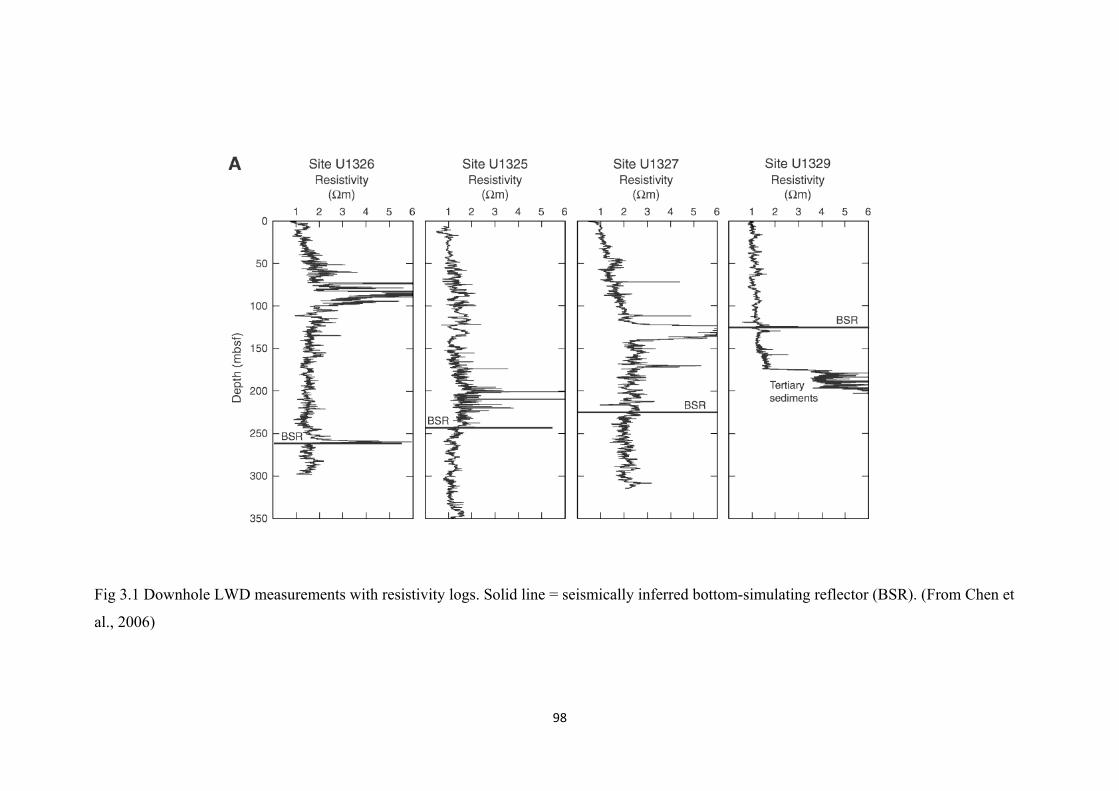
98
Fig 3.1 Downhole LWD measurements with resistivity logs. Solid line = seismically inferred bottom-simulating reflector (BSR). (From Chen et
al., 2006)

99
(a)
15 20 25 30 35 40
0
50
100
150
200
250
300
Dep
th b
elow
sea
floor
(m)
Interstitial water salinity
U1325
(b)
0 0.1 0.2 0.3 0.4
0
50
100
150
200
250
300
Dep
th b
elow
sea
floor
(m)
Interstitial water resistivity(ohm-m)
U1325
Fig 3.2 (a) Water salinity (in ppt) from recovered sediment at Hole U1325B, U1325C and U1325D (b) estimated in situ water resistivity
calculated from the equation of state of sea water (Fofonoff, 1985).

100
(a) 0.1 0.2 0.3 0.4 0.5 0.6 0.7 0.8 0.90
2
4
6
8
10U1325 Pickett Plot
LWD density-Porosity
FF(R
t/Rw
)
m=0.26, a=4.65m=1.76, a=1.17
(b)0.2 0.3 0.4 0.5 0.6 0.7 0.8 0.9 10
2
4
6
8
10U1325 Pickett Plot
core-derived porosity
FF(R
t/Rw
)
m=0.44, a=3.76m=1.76, a=1.64
Fig. 3.3 (a) Pickett Plot in Site U1325, the blue scattered points are the density-porosity values plotted against the FF data. A red power line is
then fitted through the scattered points, the empirical parameters from the equation of the power line (as showed at bottom of the chart) is a=3.48,
m=0.43, and the blue line stands for the empirical relationship calculated also from LWD density-porosity data, with m fixing to 1.76, parameter
a from empirical fitting equals to 1.17. (b) Pickett plot in Site U 1325 using the core derived density porosity values plotted against the FF data.
A power line is fitted through the scattered point, the empirical parameters is a= 3.76, m=0.44. Blue line is the power relationship between core-
derived porosity and FF with m=1.76, a=1.64.

101
0 0.1 0.2 0.3 0.4 0.5 0.6
0
50
100
150
200
250
300
350
400
Dep
th b
elow
sea
floor
(m)
Gas Hydrate Saturation
U1325
Sh (density-porosity, a=1.17, m=1.76)Sh (core-derived porosity, a=1.64,m=1.76)
0 0.1 0.2 0.3 0.4 0.5 0.6
0
50
100
150
200
250
300
350
400
Dep
th b
elow
sea
floor
(m)
Gas Hydrate Saturation
U1325
Sh (m=0.43, a=3.48)Sh (m=1.76, a=1.17)
Fig. 3.4 (a) the red line is Site U 1325 gas hydrates saturation (Sh) calculated
from LWD log-derived density-porosity data, the empirical value are a =1.17,
m=1.76, the blue line is Sh calculated from core-derived porosity with a= 1.64,
m=1.75. (b) The red line stands for the Sh calculated from LWD log-derived
density-porosity data, the empirical values are a =1.17, m=1.76, yellow line is
Sh calculated from LWD log-derived density-porosity data with m=0.43,
a=3.48. In all the calculations, the value n is chosen as 1.95.

102
(a)
5 10 15 20 25 30 35
0
50
100
150
200
250
300
Dep
th b
elow
sea
floor
(m)
Interstitial water salinity
U1326
(b)
0.15 0.2 0.25 0.3 0.35
0
50
100
150
200
250
Dep
th b
elow
sea
floor
(m)
Interstitial water resistivity(ohm-m)
U1326
Fig 3.5 (a) Water salinity (in ppt) from recovered sediment at Hole U1326C and U1326D (b) estimated in situ water resistivity calculated from
the equation of state of sea water (Fofonoff, 1985).

103
(a)0.2 0.3 0.4 0.5 0.6 0.7 0.8 0.9 10
2
4
6
8
10U1326 Pickett Plot
LWD density porosity
FF(R
t/Rw
)
m=0.26, a=4.65m=1.76, a=1.57
(b) 0.2 0.3 0.4 0.5 0.6 0.7 0.8 0.9 10
2
4
6
8
10U1326 Pickett Plot
core-derived Porosity
FF(R
t/Rw
)
m=0.23, a=4.76m=1.76, a=2.3
Fig. 3.6 (a) “Pickett Plot” in Site U1326, the blue scattered points are the density-porosity values plotted against the FF data. A power line is then
fit through the scattered points, the empirical parameters for the equation of the power line (as showed at bottom of the chart) are a=4.65,
m=0.27. The blue line stands for the empirical relationship calculated from LWD density-porosity data, with m fixing to 1.76, parameter a from
empirical fitting equals to 1.57. (b) Pickett Plot shows the results of core-derived porosity plotting against the FF data in Site U1326. A power
line is then fit through the scattered point, the empirical parameters from the equation of the power line (as showed at bottom of the chart) is
a=4.67, m=0.23. The blue line is the empirical relationship between core-derived porosity and FF from core-derived porosity with m=1.76, a=2.3.

104
(a)
0 0.2 0.4 0.6 0.8
0
50
100
150
200
250
300
Dep
th b
elow
sea
floor
(m)
Gas Hydrate Saturation
U1326
Sh (density-porosity, m=1.76, a=1.57)Sh (core-derived porosity, m=1.76,a=2.3)
(b)
0 0.2 0.4 0.6 0.8
0
50
100
150
200
250
300
Dep
th b
elow
sea
floor
(m)
Gas Hydrate Saturation
U1326
Sh (density-porosity, m=0.27,a=4.65)Sh (density-porosity, m=1.76, a=1.57)
Fig. 3.7 Gas hydrate saturation from density-porosity and core-derived porosity calculation; the yellow line stands for gas hydrate saturation
using the empirical value 4.65 and 0.27 for a and m respectively, the red line (in both (a) and (b)) stands for the gas hydrate saturation from
density-porosity using m=1.76, a =1.57. The blue line is the result from core-derived porosity, using m=1.76, a=2.3.

105
(a)
0 10 20 30 40
0
50
100
150
200
250
300
Dep
th b
elow
sea
floor
(m)
Interstitial water salinity
U1327
(b)
0.2 0.25 0.3 0.35 0.4
0
50
100
150
200
250
300
Dep
th b
elow
sea
floor
(m)
Interstitial water resistivity(ohm-m)
U1327
Fig 3.8 (a) U1327 water salinity (in ppt) derived from recovered core. Gas hydrate dissociation upon recovery is the cause of the low salinity
outliers (fresh water). (b) Estimated in situ water resistivity calculated from the equation of state of sea water (Fofonoff, 1985).

106
(a) 0.2 0.3 0.4 0.5 0.6 0.7 0.8 0.9 10
2
4
6
8
10U1327 Pickett Plot
LWD log-derived Porosity
FF(R
t/Rw
)
m=0.26, a=3.74m=1.76, a=1.27
(b) 0.2 0.3 0.4 0.5 0.6 0.7 0.8 0.9 10
2
4
6
8
10U1327 Pickett Plot
core-derived Porosity
FF(R
t/Rw
)
m=0.21, a=3.74m=1.76, a=1.27
Fig. 3.9 (a) Pickett Plot in Site U1327, the blue scattered points are the density-porosity values plotted against the FF data. A power-trendline is
then fit through the scattered points, and the empirical parameters from the equation of the best-fit trendline are a=3.74, m=0.26. The blue line
stands for the empirical relationship between LWD derived porosity and FF with m=1.76 and a=1.27. (b) Pickett Plot showing the results of
core-derived density porosity against the FF data at Site U1327. A power-trendline is then fit through the scattered points, the empirical
parameters from the equation of the best-fit trendline are a=3.74, m=0.21.

107
(a)
0 0.2 0.4 0.6 0.8
0
50
100
150
200
250
300
Dep
th b
elow
sea
floor
(m)
Gas Hydrate Saturation
U1327
Sh (density porosity, m=1.76, a=1.27)Sh (density porosity, m=0.55, a=2.99)
(b)
0 0.2 0.4 0.6 0.8
0
50
100
150
200
250
300
Dep
th b
elow
sea
floor
(m)
Gas Hydrate Saturation
U1327
Sh (core porosity, m=1.76, a=1.98)Sh (density porosity, m=1.76, a=1.27)
Fig.3.10 (a) Gas hydrate saturation from density-porosity and core-derived porosity calculation; the yellow line stands for gas hydrate saturation
calculated from core-density using the empirical value 1.98 and 1.76 for a and m respectively, the red line (in both (a) and (b)) stands for the gas
hydrate saturation from density-porosity using m=1.76, a =1.27. The blue line is the result from density- porosity, using m=0.55, a=2.99.
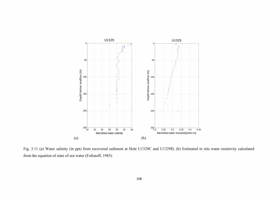
108
(a)
22 24 26 28 30 32 34
0
50
100
150
200
250
Dep
th b
elow
sea
floor
(m)
Interstitial water salinity
U1329
(b)
0.2 0.25 0.3 0.35 0.4 0.45
0
50
100
150
200
250
Dep
th b
elow
sea
floor
(m)
Interstitial water resistivity(ohm-m)
U1329
Fig. 3.11 (a) Water salinity (in ppt) from recovered sediment at Hole U1329C and U1329D, (b) Estimated in situ water resistivity calculated
from the equation of state of sea water (Fofonoff, 1985).

109
(a) 0.2 0.3 0.4 0.5 0.6 0.7 0.8 0.9 10
2
4
6
8
10U1329 Pickett Plot
LWD log-derived Porosity
FF(R
t/Rw
)
m=0.31, a=2.94m=1.76, a=1.18
(b) 0.2 0.3 0.4 0.5 0.6 0.7 0.8 0.9 10
2
4
6
8
10U1329 Pickett Plot
core-derived Porosity
FF(R
t/Rw
)
m=0.26, a=3.02m=1.76, a=1.43
Fig. 3.12 (a) Pickett Plot in Site U1329, the blue scattered points are the density-porosity values against the FF data. A power-trendline is then
fit through the scattered points, the empirical parameters from the equation of the best-fit trendline are a=2.94, m=0.31. The blue line stands for
the empirical relationship between LWD density porosity and FF with m=1.76 and a=1.18. (b) Pickett Plot showing the results of core-derived
density porosity against the FF data. A power-trendline is fit through the scattered points, and the empirical parameters from the equation of the
best-fit trendline are a=3.02, m=0.26. The blue line is the power relationship with core-derived porosity and FF with m=1.76 and a=1.43.

110
(a)
0 0.1 0.2 0.3 0.4 0.5
0
20
40
60
80
100
120
140
Dep
th b
elow
sea
floor
(m)
Gas Hydrate Saturation
U1329
Sh (density-porosity, m=1.76, a=1.43)Sh (density-porosity, m=1.76, a=1.18)
(b)
0 0.1 0.2 0.3 0.4 0.5
0
20
40
60
80
100
120
140
Dep
th b
elow
sea
floor
(m)
Gas Hydrate Saturation
U1329
Sh (density-porosity, m=0.31, a=2.94)Sh (density-porosity, m=1.76, a=1.15)
Fig. 3.13 Gas hydrate saturation from density-porosity and core-derived porosity calculation of Site U1329; the blue line stands for gas hydrate
saturation using the empirical value 2.94 and 0.31 for a and m respectively, the red line (in both (a) and (b)) stands for the gas hydrate
saturation from density-porosity using m=1.76, a =1.18. The yellow line is the result from core-derived porosity, using m=1.76, a=1.43.
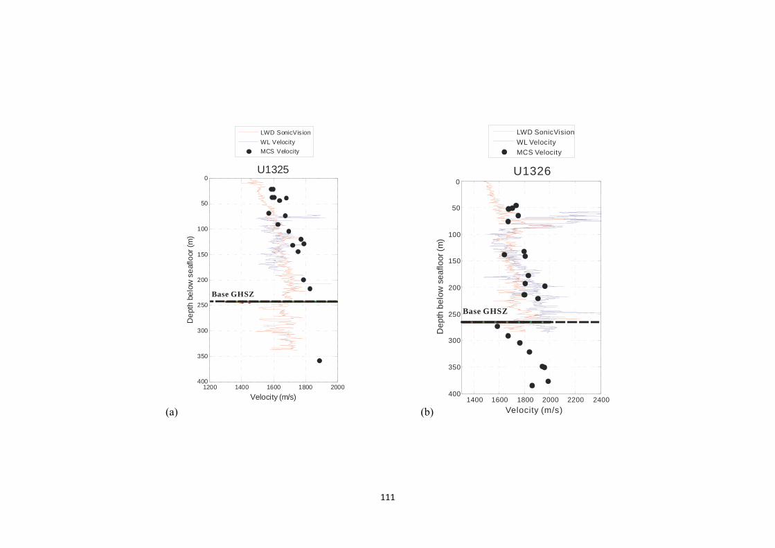
111
(a)
1200 1400 1600 1800 2000
0
50
100
150
200
250
300
350
400
Velocity (m/s)
Dep
thbe
low
seaf
loor
(m)
U1325
LWD SonicVis ionWL VelocityMCS Velocity
Base GHSZ
(b) 1400 1600 1800 2000 2200 2400
0
50
100
150
200
250
300
350
400
Dep
thbe
low
seaf
loor
(m)
Velocity (m/s)
U1326
LWD SonicVisionWL VelocityMCS Velocity
Base GHSZ

112
(c) 1300 1400 1500 1600 1700 1800 1900 2000
0
50
100
150
200
250
300
350
400
450
Dep
thbe
low
seaf
loor
(m)
Velocity (m/s)
U1327
LWD SonicVisionWL VelocityMCS Velocity
Base GHSZ
(d) 1200 1400 1600 1800 2000 2200
0
50
100
150
200
250
300
350
400
Dep
thbe
low
seaf
loor
(m)
Velocity (m/s)
U1329
LWD SonicVisionWL VelocityMCS Velocity
Base GHSZ
113
Fig. 3.14 The velocity data from the four transect drilling sites. The red line stands in all plots for the LWD velocity, which comes from the A-
Hole, the blue line is the WL velocity and the black points are the MCS velocity values. The purple line in Site U1327 stands for the
unconstrained interval velocity calculated from the VSP data. The depth of the Base of the Gas hydrate stability zone (equivalent to BSR) is
marked by the black horizontal line in each graph.

114
0 0.05 0.1 0.15 0.2 0.25 0.3
0
50
100
150
200
250
300
350
Dep
th b
elow
sea
floor
(m)
Gas hydrate saturation (fraction of pore space)
U1325
Fig.3.15 Gas hydrate saturations at Site U1325. The red line shows the results
calculated from LWD velocity data acquired from Hole U1325A.The blue line
is for the results calculated from WL velocity collected from Hole U1325C.
The black stars are the results from the MCS data calculated from the main
transect line MCS line 89-08. The location of the estimated base of GHSZ has
been marked by a thick black line.
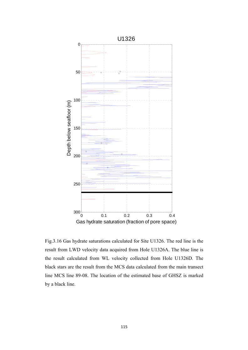
115
0 0.1 0.2 0.3 0.4
0
50
100
150
200
250
300
Dep
th b
elow
sea
floor
(m)
Gas hydrate saturation (fraction of pore space)
U1326
Fig.3.16 Gas hydrate saturations calculated for Site U1326. The red line is the
result from LWD velocity data acquired from Hole U1326A. The blue line is
the result calculated from WL velocity collected from Hole U1326D. The
black stars are the result from the MCS data calculated from the main transect
line MCS line 89-08. The location of the estimated base of GHSZ is marked
by a black line.

116
0 0.1 0.2 0.3 0.4
0
50
100
150
200
250
300
Dep
th b
elow
sea
floor
(m)
Gas hydrate saturation (fraction of pore space)
U1327
Fig.3.17 Gas hydrate saturations at Site U1327. The red line stands for the
results calculated from LWD velocity data acquired from Hole U1327A. The
blue line stands for the results calculated from WL velocity collected from
Hole U1327E. The black stars are the results from the MCS data calculated
from the main transect line MCS line 89-08. The location of the estimated
base of GHSZ has been marked in this graph.

117
0 0.1 0.2 0.3 0.4 0.5 0.6
0
20
40
60
80
100
120
140
160
180
U1329
Gas Hydrate Saturation (fraction of pore space)
Dep
th B
elow
Sea
floor
(m)
Fig. 3.18 Gas hydrate saturations for Site U1329. The red line stands for the
results calculated from LWD velocity data acquired from Hole U1329A. The
blue line stands for the results calculated from WL velocity collected from
Hole U1329D. The black stars are the results from the MCS data calculated
from the main transect line MCS line 89-08. The location of the estimated
base of GHSZ has been marked in this graph.

118
Fig. 4.1 Multibeam bathymetry map with main seismic sections used for Site
U1325 along the transect across the accretionary prism offshore Vancouver
Island (courtesy of D. Kelley, J. Delaney, and D. Glickson, University of
Washington, and C. Barnes, C. Katnick, NEPTUNE Canada, University of
Victoria; funded by the University of Washington and the W.M. Keck
Foundation). MCS = multichannel seismic
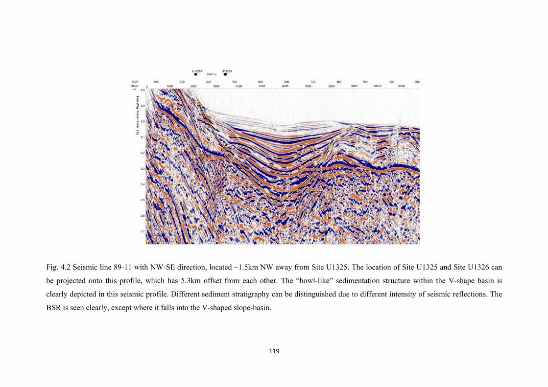
119
Fig. 4.2 Seismic line 89-11 with NW-SE direction, located ~1.5km NW away from Site U1325. The location of Site U1325 and Site U1326 can
be projected onto this profile, which has 5.3km offset from each other. The “bowl-like” sedimentation structure within the V-shape basin is
clearly depicted in this seismic profile. Different sediment stratigraphy can be distinguished due to different intensity of seismic reflections. The
BSR is seen clearly, except where it falls into the V-shaped slope-basin.

120
Fig. 4.3 Subbottom profiler data from line ODP7, the red line indicates the location of line 89-11. The transparent layer of Holocene sediment
ontop of higher reflective material can be clearly seen in this image. The layer is composed of the sediment with extremely high porosity and low
density, indicating the pelagic sedimentation on the seafloor without any influx of new turbidite sediment and compaction effects (Novosel,
2005). The vertical time scale is a reduced traveltime as a deep-water delay of 1.0 seconds was used in the recording of the 3.5 kHz profiler data.

121
Fig. 4.4 Section of MCS Line 89-08 over Site U1325. The yellow line indicates the boundary between lithostratigraphic Subunits IA and IB,
which can be traced for ~1.5km around Site U1325. The BSRs is indicated by the green line. There are several small-scale faults cutting through
the buried ridge and some of them almost extend to the BSRs.

122
Fig. 4.5 Seismic profile of MCS line ODP3, the green dashed line shows the discontinuous BSR. The buried uplifted ridge can be located in the
centre just below the projected location of Site U1325.

123
Fig. 4.6 Seismic Profile of MCS line ODP2, which is located 2.5km SE of Site U1325. The rough location of the uplifted ridge in centre is
marked by the seismic high reflectivity shown at the projected location of Site U1325. The complicated appearances of the sediments at the NE
side of the basin indicate progressive deformation inside the basin. BSRs are difficult to identify in this seismic section.

124
Fig. 4.7 Seismic Profile of MCS line ODP7. The yellow line indicates the unconformity; the deeply cutting faults within the buried ridge are
indicated by dashed black lines. The green arrow points out the location where a BSR is speculated to appear.

125
Fig. 4.8 Section of SCS line CAS02B_line05_04 over Site U1325. The green line indicates the unconformity boundary between lithostratigraphic
Subunits IA and IB, which can be traced for ~1.2 km around Site U1325. The proposed location of BSRs is indicated by the yellow line, which
was projected from observations along the other seismic profiles. The black dashed line indicates the general pattern of the sediment, which is
semi-similar to the seafloor. There are several small-scale fractures distributed inside the highly deformed sediments. Note the various side-
echoes, which have been marked by black dashed lines on the two sides of the basin.
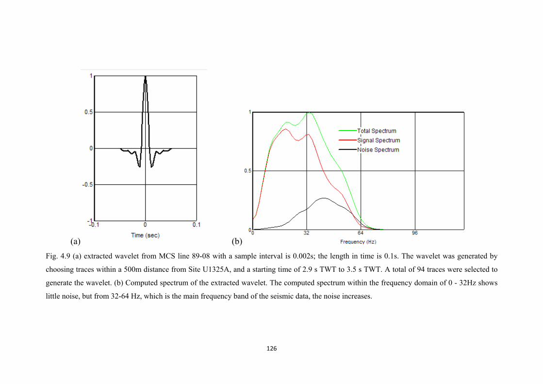
126
(a) (b) Fig. 4.9 (a) extracted wavelet from MCS line 89-08 with a sample interval is 0.002s; the length in time is 0.1s. The wavelet was generated by
choosing traces within a 500m distance from Site U1325A, and a starting time of 2.9 s TWT to 3.5 s TWT. A total of 94 traces were selected to
generate the wavelet. (b) Computed spectrum of the extracted wavelet. The computed spectrum within the frequency domain of 0 - 32Hz shows
little noise, but from 32-64 Hz, which is the main frequency band of the seismic data, the noise increases.

127

128
Fig. 4.10 Synthetic seismogram using the wavelet shown in Figure 4.10 (from MCS line 89-08). The first column is the integrated log time–
depth conversion; the second column is the computed T-D chart velocity (m/s). The following columns are the LWD velocity data, the LWD
density values from Hole U1325A, computed acoustic impedance (AI), and reflection coefficients (RC). The extracted wavelet is shown used in
the convolution to produce the synthetic traces (both polarities are shown). The resistivity is used as the reference log here. The seismic trace
extracted from line 89-08 at U1325 is shown giving a correlation coefficient of 0.42. The location of the BSR is marked by the yellow dashed
line. The synthetic seismogram in the zone indicated by the two green dashed lines has relatively low reliability because of the abnormally low
density values from the LWD log, which may be caused by degraded borehole conditions.

129

130
Fig. 4.11 The seismic profile of MCS line 89-08 with generated synthetic seismogram, logging data, core pore-fluid chlorinity data and
lithologic units. The first column shows the pore-fluid chlorinity data. The second column shows the resistivity data (the red line stands for
U1325A LWD data and the green line stands for U1325C WL data). The gray bar is showing the lithologic units. The column with red wiggle
line inside is the synthetic generated from the MCS 89-08 seismic data convolved with LWD velocity and density data. The column following is
the velocity data (the red line stands for the WL logging data, the green line is the MCS velocity). The last column includes the gas hydrate
saturation calculated from LWD resistivity data.

131
Fig. 4.12 The seismic profile of MCS line ODP7 with generated synthetic seismogram, logging data, core-derived pore-fluid chlorinity data and
lithologic units. Pattern of data shown is identical to those shown in Fig. 4.12.

132
Fig. 4.13 Bathymetry map and seismic lines used at Site U1326; (courtesy of D. Kelley, J. Delaney, and D. Glickson, University of Washington,
and C. Barnes, C. Katnick, NEPTUNE Canada, University of Victoria; funded by the University of Washington and the W.M. Keck Foundation).

133
Fig. 4.14 Seismic profile of SCS line CAS03B_inline01, the red vertical line marks the location of CAS03B Xline10 which almost goes through
the Site U1326. The BSR is marked in the graph and the location of the slump is pointed out by the arrow.

134
Fig.4.15 Profile of SCS line CAS03B-Xline01. The BSR is indicated by the yellow dashed line. The vertical red line indicates the location of the
intersecting MCS line CAS3MCS99 (shown in Fig. 4.18).

135
Fig. 4.16 Seismic profile of SCS line CAS03_Xline03. The BSR has been marked in the graph by the black dashed line which extends from SP
140-200. The red line is also the location of the transect line CAS3MCS99. The location of the U1326A is marked at the top.

136
Fig. 4.17 Seismic profile MCS line 89-08, the red line marks the location of seismic line CAS3MCS99, which is roughly the location of Site
U1326. The BSR is indicated with a yellow dashed line. The green dashed line inside the frontal basin is the boundary between the well-bedded
and slightly uplifted sediment layers.

137
Fig. 4.18 Section of MCS line CAS3MCS99 crossing the ridge in a southeast–northwest direction. A series of faults is clearly visible, which are
indicated by black dash lines, resulting in a seafloor displacement of up to 25 m. A possible slope slump (additional to the main slump already
identified earlier) is indicated by the yellow line on the seafloor, and the black arrow points out the location of the BSR. The locations of Hole
U1326A and the originally proposed site CAS-03B have been marked on the top.

138
(a) (b)
Fig. 4.19 (a) extracted wavelet from MCS line CAS03MCS99 with a sample interval of 0.002s; the length in time is 0.1s. The wavelet is
generated from traces within a 300m distance from Site U1326A, with a time range of 2.5 s TWT to 2.95 s TWT. A total of 247 traces were
selected to generate the wavelet. (b) Computed spectrum of the extracted wavelet. The computed spectrum within the frequency domain of 0 -
192Hz shows little noise, except within the frequency band of 32-64 Hz.

139

140
Fig. 4.20 Synthetic seismogram using the wavelet shown in Figure 4.20 (from MCS line CAS3MCS99). The first column is the integrated log
time –depth conversion; the second column is the computed T-D chart velocity (m/s). The following columns are the LWD velocity data from
Hole U1326A, computed acoustic impedance (AI), and reflection coefficients (RC). The extracted wavelet is shown used in the convolution to
produce the synthetic traces (both polarities are shown left and right of the real seismic trace). The gas hydrate enrichment zone and the depth of
the BSR have been marked out by the yellow dashed lines. The seismic trace was extracted from MCS line CAS3MCS99 at Site U1326 are
shown giving an overall correlation coefficient of 0.52 to the synthetics.

141

142
Fig. 4.21 Detailed multibeam bathymetry map around Site U1327 and Cold Vent Site U1328 (also known as Bullseye Vent). The location of the
main MCS 3-D grid is indicated by a yellow box; the 1999 vent field SCS grid and the 2000 SCS grid around Bullseye Vent are indicated in
black boxes. The orange dots show the location of Site U1325, Site U1327 and Site U1328. The orange line shows the main transect line MCS
89-08. The survey focuses within the two relatively topography high, which goes a NW-SE direction on the base map. The green line has pointed
out the westward dipping thrust fault.

143
Fig. 4.22 Detailed multibeam bathymetry map around Site U1327 and Cold Vent Site U1328 (also known as Bullseye Vent). The location of the
main MCS 3-D grid is indicated by a yellow box; the 1999 vent field SCS grid and the 2000 SCS grid around Bullseye Vent are indicated in
black boxes. The orange dots show the location of Site U1325, Site U1327 and Site U1328. The survey focuses within the two topographic highs,
which are in a NW-SE direction. The green line has pointed out the westward dipping thrust fault. (courtesy of D. Kelley, J. Delaney, and D.
Glickson, University of Washington, and C. Barnes, C. Katnick, NEPTUNE Canada, University of Victoria; funded by the University of
Washington and the W.M. Keck Foundation).

144
Fig.4.23 Seismic profile of MCS line 8908 around site U1327, the location of Site U1327A is projected onto this line. The steeply westward
dipping thrust fault is indicated by the black dashed line. A strong and continuous BSR can be seen from the mid-slope to the thrust fault outcrop.
The green arrows point out the ridges of accreted sediments.

145
Fig. 4.24 Seismic profile of MCS99_Inline38 of the 3D grid. The BSR has been marked by a yellow line. The location of Site U1327A is
indicated on top of the image. The NW boundary of the sediment-filled basin has been marked by a green dashed line, and small scale faults
located within the basin near CDP 200 are shown by black dashed lines.

146
Fig. 4.25 Seismic line 2008007PGC DTSEXT060, Huntec envelope data. The orange dashed line marks the boundary between the first and the
second layers, the green line indicates the boundary between the second and the third layer. A deep-water delay of 1.465s was used to record the
Huntec data. The red vertical line is the intersection point with MCS99_Inline38.

147
Fig.4.26 Seismic line PGC007-2008-line60 showing the airgun data. The red vertical line indicates the location of MCS Inline 38. The BSR
depth is marked in the figure by arrows (vertical time is reduced by a deep-water delay).

148
Fig. 4.27 Seismic line 2008007PGCDTSEX058 with Huntec envelope data. The red vertical line is MCS Inline 38.

149
Fig. 4.28 Seismic line PGC007-2008line 58 profile showing airgun data; The BSR is highlighted by the arrows.

150
(a) (b)
Fig. 4.29 (a) extracted wavelet from MCS Inline38 with a sample interval is 2ms; the total length is 0.1 s. The wavelet was generated from traces
within 200 m distance from Site U1327A, with a time window of 1.8 s TWT to 2.15 s TWT. A total of 40 traces were selected to generate the
wavelet. (b) Computed spectrum of the extracted wavelet. The computed spectrum within the frequency domain of 0 – 192 Hz shows relatively
high noise levels, especially at ~100 Hz, which is the main frequency band of the seismic data.

151

152
Fig. 4.30 Synthetic seismogram generated using the wavelet shown in Figure 4.29 (from MCS Inline38). The first column is the integrated log
time –depth conversion; the second column is the computed T-D chart velocity (m/s). The following columns are the LWD velocity data, the
LWD density values from Hole U1327A, computed acoustic impedance (AI), and reflection coefficients (RC). The extracted wavelet is used to
produce the synthetic traces (both polarities are shown). The seismic trace closest to the borehole was extracted from MCS Inline38 at U1327
and is repeated five times for easier visual comparison. A correlation coefficient of 0.179 is achieved without adjustment of the synthetic traces.

153

154
Fig. 4.31 Seismic MCS99_Inline38 profile with logging and core derived information as well as the synthetic seismogram superimposed. The
first column is the pore-fluid chlorinity profile. The second column shows the resistivity log-data (the red line is for U1327A LWD data and the
green line stands for U1327E WL data). The gray bar is showing the lithologic units. At the exact borehole location the synthetic trace is
superimposed. The next column shows the velocity data (the red line stands for the WL logging data, the green line is the VSP interval velocity).
The last column shows the gas hydrate saturation calculated from LWD resistivity data. BSR has been traced by the red line inside the graph.

155
Figure 4.32 Image showing the heterogeneity of the high-concentration zone
of Site U1327. Shown are (from left to right) LWD RAB image and extracted
ring-resistivity log, Infra-red image of the recovered core of Hole U1327C,
electrical WL log and Infra-red image of the recovered core of Hole U1327D,
and WL log of Hole U1327E. The distance between all boreholes is 60m. The
high-concentration zone (seen as bright zone in the RAB image and dark-blue
colors in the IR image) thins to the east and is entirely lost in Hole U1327E.

156
(a) (b)
Fig. 4.33 (a) extracted wavelet from MCS line8908 with a sample interval is 2ms; the total length is 0.1s. The wavelet was generated from traces
within 500m distance from Site U1327A, with a time window of 1.7s TWT to 2.2 s TWT. (b) Computed spectrum of the extracted wavelet. The
computed spectrum within the frequency domain of 0 - 64Hz shows relatively very low noise levels, except at frequency ~40Hz where the noise
ratio reaches ~10%.

157

158
Fig. 4.34 Synthetic seismogram using the wavelet shown in Figure 4.39 (from MCS line 8908). The first column is the integrated log time –
depth conversion; the second column is the computed T-D chart velocity (m/s) which is identical as for line MCS99_inline38. The following
columns are the velocity data from LWD velocity measurement, the LWD density values from Hole U1327A, computed acoustic impedance
(AI), and reflection coefficients (RC). The extracted wavelet is used to produce the synthetic traces (both polarities are shown). The seismic trace
closest to the borehole was extracted from MCS line8908 at U1327 and is repeated five times for easier visual comparison. A correlation
coefficient of 0.106 is achieved without further adjustment of the synthetic traces. The gas hydrate enrichment region and the depth of BSR have
been marked out by the yellow dashed lines. The green circle shows the part of the LWD data where some data points in the velocity have been
removed due to poor data quality. Note that the corresponding density data also show some degradation (low values). The synthetic seismogram
thus yields a false reflection event. However, the location of the poor data quality coincides with the depth range of the BSR (borehole condition
may be degraded at the transition from some hydrate-bearing sediment to free gas bearing sediment).
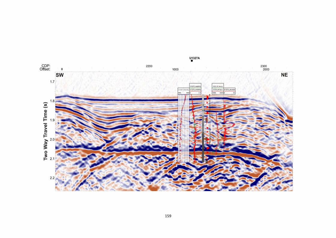
159

160
Fig. 4.35 Seismic MCS line 8908 profile with logging and core derived information as well as the synthetic seismogram superimposed. The first
column is the pore-fluid chlorinity profile. The second column is showing the resistivity log-data (the red line is for U1327A LWD data and the
green line stands for U1327E WL data). The gray bar is showing the lithologic units. At the exact borehole location the synthetic trace is
superimposed. The next column is the showing velocity data (the red line stands for the WL logging data, the green line is the VSP interval
velocity). The last column shows the gas hydrate saturation calculated from LWD resistivity data. BSR has been traced by the red line inside the
graph.

161

162
Fig. 4.36 Seismic profile of SCS line PGC007-2008line60 (airgun data) with logging and core derived information as well as the synthetic
seismogram generated from MCSinline38. The first column is the pore-fluid chlorinity profile. The second column is showing the resistivity log-
data (the red line is for U1327A LWD data and the green line stands for U1327E WL data). The gray bar shows the lithologic units. At the exact
borehole location the synthetic trace is superimposed. The next column shows the velocity data (the red line stands for the WL logging data, the
green line is the VSP interval velocity). The last column shows the gas hydrate saturation calculated from LWD resistivity data.

163
Fig. 4.37 Multibeam bathymetry map shows the northeast end of the accretionary prism on Northern Cascadia, offshore Vancouver Island.
(courtesy of D. Kelley, J. Delaney, and D. Glickson, University of Washington, and C. Barnes, C. Katnick, NEPTUNE Canada, University of
Victoria; funded by the University of Washington and the W.M. Keck Foundation). Site U1329 is indicated by the orange circle, transect MCS
line 89-08 which goes through the drilling site is shown as the red line.

164
Fig. 4.38 Seismic line CAS05C_line03 added with lithology bar. The BSR can be clearly traced for ~2.5km and extends from CDP 120 to 280.
The location of the MCS Line 89-08 is indicated for reference.

165
Fig. 4.39 MCS line 89-08 across Site U1329 with lithology units superimposed. The BSR can be traced identified in the SW portion of the line,
but it is progressively lost towards the NE into shallower water. The unconformity at Site U1329 (boundary between lithologic units II and III) is
close to the BSR at Site U1329 and thus a more complex interference pattern can be seen in the low-frequency data than in the higher-frequency
SCS data shown in Figure 4.38. The locations of the SCS lines are indicated for reference.

166
Fig. 4.40 Seismic profile of COAMS MCS99 data of ODP1. The BSR can be tracked both at the SW edge of the basin and around Site U1329.
The unconformity boundaries between different sedimentary strata have been marked out by the yellow dashed line. Strong seismic reflectivity is
seen at the NE edge of the basin which may be an indicator of free gas.

167
(a) (b)
Fig. 4.41 (a) extracted wavelet from MCS line 89-08 with a sample interval of 0.002 s; the length in time is 0.1 s. The wavelet generated by
choosing traces within 500m distance from Site U1329A, with a starting time of 1.25 s TWT to 2.0 s TWT. A total of 41 traces were selected to
generate the wavelet. (b) Computed spectrum of the extracted wavelet. The two frequency peaks reach respectively at ~24 Hz and 36 Hz. The
signal to noise ration is almost equal to 1.

168

169
Fig. 4.42 Synthetic seismogram using the wavelet shown in Figure 4.41 from MCS line 89-08. The first column shows the location of data points
(in time) used as log time–depth function; the second column is the computed T-D chart velocity (m/s). The following columns are the LWD
velocity log, the LWD density values from Hole U1329A, computed acoustic impedance (AI), and reflection coefficients (RC). The extracted
wavelet is used in the convolution to produce the synthetic traces (both polarities are shown.) The seismic traces extracted from line 89-08 at
U1329 yield a correlation coefficient with the synthetic seismogram of 0.3.

170

171
Fig. 4.43 The seismic profile of line 89-08 with generated synthetic seismogram, logging data, chlorinity data and lithologic units. The first
column stands for chlorinity data. The layers with dispersed fresher data intermingle inside the whole sediment. The second column stands for
the resistivity data, the red line stand for U1329A LWD data. The column with yellow wiggle line is the synthetic generated from MCS seismic,
LWD velocity and density data. The column following is the velocity, the red line stand for the WL logging data, the green line is the MCS
velocity. The last column includes the gas hydrate saturation we calculated from LWD resistivity data.

172
(a) (b)
Fig. 4.44 (a) extracted wavelet from CAS05B_line03 with a sample interval of 0.002s; the length in time is 0.1 s. The wavelet generated by
choosing traces within 200 m distance from Site U1329A, with a starting time of 1.2 s TWT to 1.7 s TWT. (b) Computed spectrum of the
extracted wavelet. The noise ratio reaches 0.3 at 120 Hz. However, when signal is strongest at ~70 Hz, the noise ratio is low.

173

174
Fig. 4.45 Synthetic seismogram using the wavelet shown in Fig. 4.43(a) from SCS line CAS05B_03. The first column shows the location of data
points (in time) used as log time–depth function; the second column is the computed T-D chart velocity (m/s). The following columns are the
LWD velocity log, the LWD density values from Hole U1329A, computed acoustic impedance (AI), and reflection coefficients (RC). The
extracted wavelet is shown used in the convolution to produce the synthetic traces (both polarities are shown.) The seismic traces extracted from
line CAS05B_line03 at U1329 yield a correlation coefficient with the synthetic seismogram of 0.7.

175

176
Fig. 4.46 The seismic profile of line CAS05B_line03 with generated synthetic seismogram, logging data, chlorinity data. The first column
stands for chlorinity data. The second column is stands for the resistivity data fromU1329A LWD data. The column with red wiggle line
inside is the synthetic generated from SCS seismic, LWD velocity and density data. The column following is the velocity, the red line stand
for the WL logging data, the green line is the MCS velocity generated from line8908. The last column includes the gas hydrate saturation we
calculated from LWD resistivity data.

177
(a) (b)
Fig. 4.47 (a) extracted wavelet from line ODP1MCS99 with a sample interval of 0.002 s; the length in time is 0.1 s. The wavelet is generated by
choosing traces within 200 m distance from Site U1329A, with a starting time of 1.2 s TWT to 1.65 s TWT. (b) Computed spectrum of the
extracted wavelet. The noise ratio reaches 0.3 at ~70 Hz.

178
179
Fig. 4.48 Synthetic seismogram generated from ODP1MCS99. The first column shows the location of data points (in time) used as log time–
depth function; the second column is the computed T-D chart velocity (m/s). The following columns are the LWD velocity log, the LWD density
values from Hole U1329A, computed acoustic impedance (AI), and reflection coefficients (RC). The extracted wavelet is shown used in the
convolution to produce the synthetic traces (both polarities are shown). The seismic traces extracted from line ODP1MCS99 at U1329 yield a
correlation coefficient with the synthetic seismogram of ~0.7.

180

181
Fig. 4.49 The seismic profile of line ODP1MCS99 with generated synthetic seismogram, logging data, chlorinity data and lithologic units. The
first column is the chlorinity data. The second column is the LWD resistivity data from Hole U1329A. The synthetic trace generated is shown in
yellow. The following column is velocity data (the red line is the WL logging data, the green line is the MCS velocity generated from MCS line
89-08). The last column includes the gas hydrate saturation calculated from LWD resistivity data.

182
(a)
0 0.1 0.2 0.3 0.4 0.5 0.6
0
50
100
150
200
250
300
350
400
U1325
Gas Hydrate Saturation (fraction of pore space)
Dep
th B
elow
Sea
floor
(m)
LWD v elocityLWD resistiv ity m=0.43, a=3.48
LWD resistiv ity m=1.76,a=1.17
(b)
0 0.1 0.2 0.3 0.4 0.5 0.6
0
50
100
150
200
250
300
U1326
Gas Hydrate Saturation (fraction of pore space)
Dep
th B
elow
Sea
floor
(m)
LWD velocityLWD resistivity m=0.27, a=4.65LWD resistivity m=1.76,a=1.57
(c)
0 0.1 0.2 0.3 0.4 0.5 0.6
0
50
100
150
200
250
300
U1327
Gas Hydrate Saturation (fraction of pore space)
Dep
th B
elow
Sea
floor
(m)
LWD velocityLWD resistivity m=0.26, a=3.74LWD resistivity m=1.76,a=1.27
(d)
0 0.1 0.2 0.3 0.4 0.5 0.6
0
20
40
60
80
100
120
140
160
180
U1329
Gas Hydrate Saturation (fraction of pore space)
Dep
th B
elow
Sea
floor
(m)
LWD velocityLWD resistivity m=0.31, a=2.94LWD resistivity m=1.76,a=1.18
Figure 5.1 Comparison of gas hydrate saturation estimates from logging data
(resistivity and velocity) at all four transect sites of IODP Expedition 311. The
depth of the BSR is indicated as horizontal dashed line.

183
Tables
Hole Latitude Longitude Water depth (mbsl)
Cores (N)
Cored (m)
Recovered (m)
Recovery (%)
Drilled (m)
Penetration (m)
U1325A 48°38.691′N 126°58.991′W
2201.1 0 0 0.00
350.0 350.0
U1325B 48°38.694′N 126°58.999′W 2194.8 28 205.5 141.17 68.7 1.0 206.5
U1325C 48°38.701′N 126°59.007′W 2194.8 15 115.5 62.49 54.1 188.8 304.3
U1325D 48°38.701′N 126°59.007′W 2194.6 1 4.7 4.69 99.8 0.0 4.7
Site U1325 totals: 44 325.7 208.35 64.0 539.8 865.5
U1326A 48°37.635′N 127°3.029′W
1828.1 0 0 0.00
300.0 300.0
U1326B 48°37.638′N 127°3.023′W 1828.4 1 1.5 1.55 103.3 0.0 1.5
U1326C 48°37.638′N 127°3.023′W 1828.0 13 85.7 54.39 63.0 1.0 86.7
U1326D 48°37.628′N 127°3.043′W 1827.9 20 192.6 121.96 63.3 107.4 300.0
Site U1326 totals: 34 279.8 177.9 229.6 408.4 688.2
U1327A 48°41.887′N 126°51.921′W 1322.1 0 0 0.00
300.0 300.0
U1327B 48°41.889′N 126°51.914′W 1306.1 1 9.5 9.79 103.1 0.0 9.5
U1327C 48°41.889′N 126°51.914′W 1304.5 35 297 262.17 88.3 3.0 300.0
U1327D 48°41.895′N 126°51.906′W 1303.7 17 75.9 53.99 71.1 224.1 300.0
U1327E 48°41.900′N 126°51.896′W 1303.4 4 12.5 12.37 99.0 287.5 300.0
Site U1327 totals: 57 394.9 338.32 85.7 814.6 1209.5
U1328A 48°40.072′N 126°51.022′W
1268.1 0 0 0.00
300.0 300.0
U1328B 48°40.048′N 126°51.056′W 1267.8 10 54.5 39.65 72.8 2.0 56.5
U1328C 48°40.057′N 126°51.044′W 1267.7 27 242.5 195.64 80.7 57.5 300.0
U1328D 48°40.067′N 126°51.020′W 1266.7 3 15 10.03 66.9 0.0 15.0
U1328E 48°40.080′N 126°50.987′W 1264.7 13 49 13.33 27.2 186.0 235.0
Site U1328 totals: 53 361 258.65 71.6 545.5 906.5
U1329A 48°47.369′N 126°40.713′W 959.1 0 0 0.00
220.0 220.0
U1329B 48°47.375′N 126°40.720′W 953.0 1 9.5 10.02 105.5 0.0 9.5
U1329C 48°47.375′N 126°40.720′W 946.4 23 187.5 186.16 99.3 2.0 189.5
U1329D 48°47.362′N 126°40.716′W 946.4 1 9.5 1.03 10.8 201.0 210.5
U1329E 48°47.385′N 126°40.716′W 945.5 10 48 37.74 78.6 79.0 127.0
Site U1329 totals: 35 254.5 234.95 92.3 502.0 756.5
Table 2.1 Expedition 311 operations summary for location of boreholes, and penetration depths (from Riedel et al. 2005)
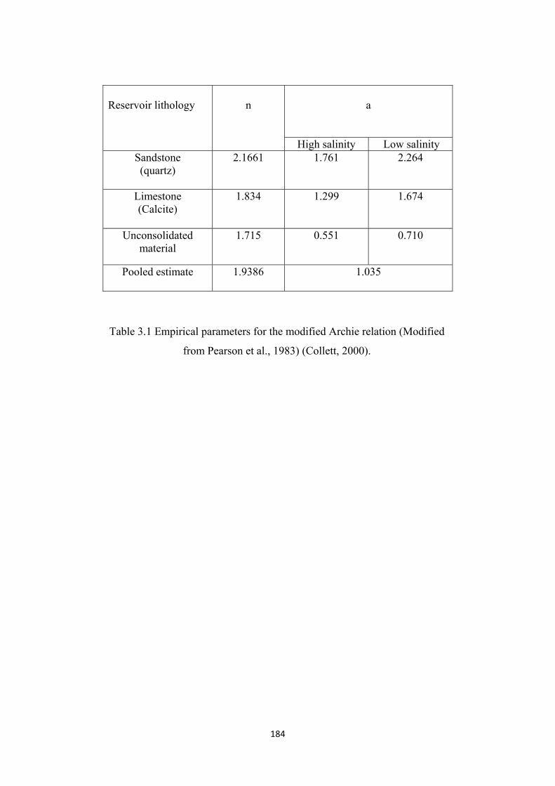
184
a
Reservoir lithology
n
High salinity Low salinity Sandstone (quartz)
2.1661 1.761 2.264
Limestone (Calcite)
1.834 1.299 1.674
Unconsolidated material
1.715 0.551 0.710
Pooled estimate 1.9386 1.035
Table 3.1 Empirical parameters for the modified Archie relation (Modified
from Pearson et al., 1983) (Collett, 2000).
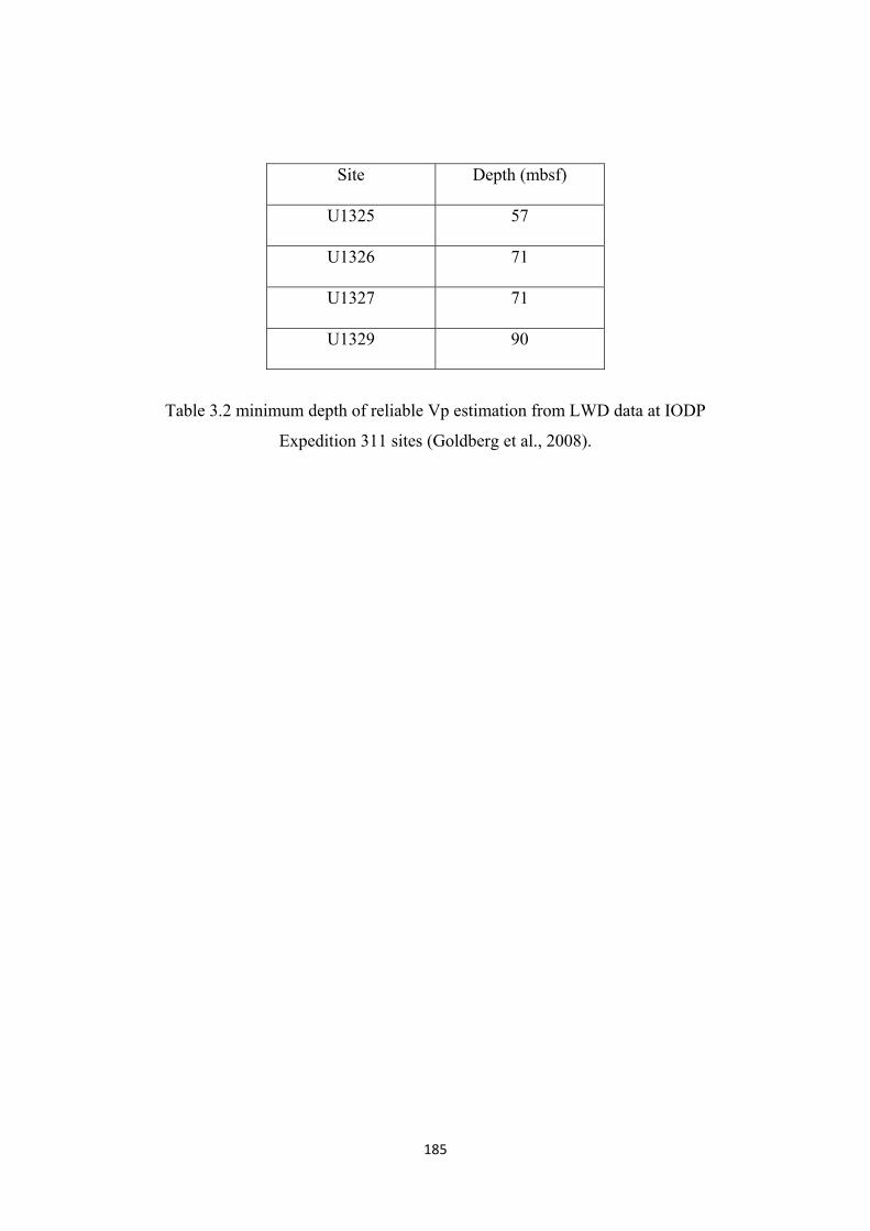
185
Site Depth (mbsf)
U1325 57
U1326 71
U1327 71
U1329 90
Table 3.2 minimum depth of reliable Vp estimation from LWD data at IODP
Expedition 311 sites (Goldberg et al., 2008).

186
Reservoir
constituent
Vp
(km/s)
Vs
(km/s)
Bulk-
density
(g/ 3cm )
Bulk
moduli
(K,
Mpa)
Shear
moduli
(G, Mpa)
Reference
Methane hydrate
structure- Ι
3.35* 1.68** 0.9 6713*** 2540*** *Estimated from Whiffen et al. (1982),
**Estimated from Pandit and King (1982),
***Calculated fromVp-Vs
Pure water 1.5 0.00 1.03 2250 0 Schlumberger Educational Services (1989)
Ice 3.8 2.00 0.92 8400 3700 King (1984)
Quartz 5.98 4.04 2.65 38000 44000 Toksoz et al. (1976)
Clay 3.40 1.60 2.60 21200 6666 Tosaya and Nur (1982)
Marine sediment 4.37 2.60 2.75 27200 18300 Lee et a. (1996)
Table 3.3 Acoustic velocity, elastic constants, and bulk-densities for various reservoir constituents.

187
1325A 1325C 1326A 1326D 1327A 1327D 1327E 1329A 1329C 1329D
Pre-cruise seismic BSR [mbsf] * 230 234 223 125
(a) Water Depth (m) 2196 1828 1308 950
(a) Distance from Deformation
Front (km) 11 5 21 38
(a)Depth below seafloor [s] TWT 0.2883 0.2817 0.272 0.154
(a) LWD-Rt 240 * 260 * 230 * * n.d. * *
(a)CWL-Vp * d.n.r.b * 260 * * 228 * * 125
(a)CWL-Rt * d.n.r.b. * 260 * 235 235 * * 125
(a)Deepest Cl− anomaly * 238.9 * 264 * 222 * * 128 *

188
(a)C1/C2 * 243 * * * 225 * * 119 *
(a)i-C4/n-C4 or C3 * * * * * 225 * * * *
(a)VSP * * * * * 245 * * * *
(a)Best estimate of BGHSZ 240.5
264 230 124
(b)Thickness of the GHOZ (m)
168
217
119
0
(c)Thickness of potential GHOZ
(m)
238
261
221
113
Table 4.1. Summary of Site-information for the individual boreholes of all four transect sites including water depth, distance to deformation front,
and estimated BSR depth using various techniques. * Velocity used for BSR depth conversion from TWT: 1636 m/s maximum average velocity
from seafloor to BSR; 1619 m/s minimum average from seafloor to BSR, reported depth is average between min and max estimate; note that
velocity was determined from VSP at ODP Site 889, n.d. Not detected, d.n.r.b. Wire-line logging tools did not reach BSR depth. (a) from
Riedel et al. (2006) , (b) from Malinverno et al. (2008), (c) from Pohlman et al. (2008).

189
TVD (Seismic)(meter) Time (2-way travel time)(s) 2201.195 2.93987 2221.942 2.9678
2237 2.98666 2239.036 2.99312
2241 2.99912 2246.806 3.00762
2250 3.01244 2258.719 3.03072
2260 3.03344 2262 3.03527
2272.188 3.04068 2276 3.04261 2288 3.05979
2300.16 3.08261 2307 3.09502
2310.002 3.09835 2311 3.09943
2321.398 3.10275 2329 3.10513
2331.758 3.10619 2345.744 3.11172
2347 3.11221 2349 3.11348 2350 3.11423 2351 3.11528 2353 3.11724 2354 3.11804 2357 3.11994 2375 3.12994
2377.342 3.13184 2378 3.13237 2395 3.1456
2405.313 3.15455 2412 3.16023 2414 3.16198 2417 3.1646 2419 3.16627
2423.444 3.17021 2445 3.18914
2461.258 3.20544 2465 3.20916 2466 3.21014 2467 3.21109
2500.108 3.24677 2541.548 3.29102 2559.16 3.30971
Table 4.2 Time-Depth Chart in U1325.

190
TVD (Seismic) (Meters) Time (TWT) (s) 1829 2.50457
1830.1 2.50567 1838 2.51322 1844 2.51998
1848.1 2.52428 1852 2.52831 1853 2.5293 1854 2.53055 1859 2.53711
1860.1 2.53865 1864 2.544 1869 2.55429 1870 2.55529 1871 2.55607
1871.6 2.55654 1876 2.55992 1879 2.56197
1881.1 2.56341 1883 2.56472 1885 2.56627
1886.1 2.56831 1890 2.58302 1891 2.58413
1895.1 2.58543 1899 2.58669
1900.1 2.58888 1901.6 2.59139 1905.1 2.59809 1907.6 2.60273 1909 2.60554
1909.6 2.6067 1910 2.60734 1911 2.60832
1912.1 2.60973 1915.6 2.61418 1918 2.61759
1919.1 2.61915 1920 2.62046
1928.6 2.62822 1936.1 2.63526 1939 2.6381
1940.6 2.64049 1941 2.64106 1946 2.64872 1953 2.65704 1956 2.66024 1957 2.66159
1959.6 2.66495

191
1971 2.68011 1972 2.68171
1972.6 2.68264 1977 2.68928
1978.6 2.69298 1980 2.69623 1981 2.6976 1982 2.69844
1983.1 2.6994 1993 2.70793 2000 2.71869
2001.6 2.72128 2009 2.73299 2013 2.73652 2014 2.73775
2015.1 2.73893 2021 2.74528 2022 2.74636 2030 2.75455
2033.1 2.75794 2034 2.75899 2035 2.76015
2036.1 2.76259 2040.1 2.77497 2044 2.78194 2045 2.78329 2047 2.7845
2049.1 2.78567 2053.1 2.79396 2055.1 2.79828 2059 2.80315 2061 2.80444 2071 2.81045
2072.1 2.8114 2078.1 2.81734 2081.6 2.82077 2084 2.8231 2085 2.82415
2086.6 2.82583 2089.1 2.82809 2091 2.83016 2095 2.83482
2100.6 2.84154 2102 2.84321
2104.6 2.84621 2109.1 2.85144 2112.1 2.85483
2326.126 3.10788
Table 4.3 Time-Depth Chart for Site U1326.

192
TVD(seismic) (meters) Time(TWT)(s) 1322.226 1.76973 1325.6 1.77425 1342.6 1.79758 1354.6 1.81364 1373.1 1.83804 1386.1 1.85496 1396.1 1.86803 1399.1 1.87175 1417.6 1.89528 1432.6 1.91406 1435 1.91699 1441 1.93033
1444.6 1.9344 1447.6 1.93765 1451.1 1.94096 1460.1 1.94948 1464.6 1.95393 1494.1 1.98612 1499.1 1.9914 1506.6 1.99951 1514.1 2.00761 1524.6 2.01528 1533.6 2.02154 1538.1 2.02473 1543 2.02818 1545 2.02995
1546.1 2.03104 1549 2.03396
1554.1 2.03975 1566.6 2.05512 1579.6 2.07149 1588.1 2.08236 1590.6 2.0853 1594.1 2.0896 1598.1 2.09478 1605.1 2.1032 1608.6 2.10733 1613.6 2.11342 1618.1 2.11852 1624.1 2.12556 1626 2.12783 1626 2.12783 1626 2.12783
1625.6 2.12735
Table 4.4 Time Depth Chart for Site U1327.

193
TVT (seismic) (meters) TWT (s) 959.64 1.27408
963.145 1.27881 973.673 1.29302 987.167 1.31084 1001.74 1.32969
1015.774 1.34751 1034.125 1.37003
1050 1.38918 1052 1.39401
1054.636 1.39687 1072 1.41549 1082 1.42742
1099.435 1.44194 1115 1.45507 1116 1.45607
1123.724 1.46428 1128 1.46886 1131 1.47193 1132 1.47312 1133 1.47432 1135 1.47664 1216 1.57528
1216.45 1.57583
Table 4.5 Time-Depth Chart in U1329.
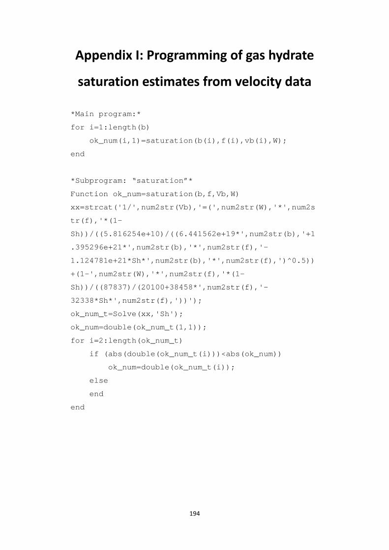
194
Appendix I: Programming of gas hydrate
saturation estimates from velocity data
*Main program:*
for i=1:length(b)
ok_num(i,1)=saturation(b(i),f(i),vb(i),W);
end
*Subprogram: “saturation”*
Function ok_num=saturation(b,f,Vb,W)
xx=strcat('1/',num2str(Vb),'=(',num2str(W),'*',num2s
tr(f),'*(1-
Sh))/((5.816254e+10)/((6.441562e+19*',num2str(b),'+1
.395296e+21*',num2str(b),'*',num2str(f),'-
1.124781e+21*Sh*',num2str(b),'*',num2str(f),')^0.5))
+(1-',num2str(W),'*',num2str(f),'*(1-
Sh))/((87837)/(20100+38458*',num2str(f),'-
32338*Sh*',num2str(f),'))');
ok_num_t=Solve(xx,'Sh');
ok_num=double(ok_num_t(1,1));
for i=2:length(ok_num_t)
if (abs(double(ok_num_t(i)))<abs(ok_num))
ok_num=double(ok_num_t(i));
else
end
end