study of land cover changes of baghdad using multi ... · study of land cover changes of baghdad...

Al-Abudi et al. Iraqi Journal of Science, 2016, Vol. 57, No.3B, pp:2146-2160

_______________________________

*Email: [email protected]

2146

Study of Land Cover Changes of Baghdad

Using Multi-Temporal Landsat Satellite Images

Bushra Q. Al-Abudi1, Mohammed S. Mahdi

2, Yasser Chasab Bukheet

1*

1Astronomy and Space Department, College of Science, Baghdad University, Baghdad, Iraq 2Computer Science Department, College of Science, Al-Nahrain University, Baghdad, Iraq

Abstract

The main goal of this work is study the land cover changes for "Baghdad city"

over a period of (30) years using multi-temporal Landsat satellite images (TM,

ETM+ and OLI) acquired in 1984, 2000, and 2015 respectively. In this work, The

principal components analysis transform has been utilized as multi operators, (i.e.

enhancement, compressor, and temporal change detector). Since most of the image

band's information are presented in the first PCs image. Then, the PC1 image for all

three years is partitioned into variable sized blocks using quad tree technique.

Several different methods of classification have been used to classify Landsat

satellite images; these are, proposed method singular value decomposition (SVD)

using Visual Basic software and supervised method (Maximum likelihood

Classifier) using ENVI 5.1 software are utilized in order to get the most accurate

results and then compare the results of each method and calculate the land cover

changes that have been taken place in years 2000 and 2015; comparing with 1984.

The image classification of the study area resulted into five land cover types: Water

body, vegetation, open land (Barren land), urban area "Residential I" and urban area

"Residential II". The results from classification process indicated that water body,

vegetation, open land and the urban area "Residential I" are increased, while the

second type from urban area "Residential II" in decrease to year 2015 comparable

with 1984. Despite use of many methods of classification, results of the proposed

method proved its efficiency, where the classification accuracies for the (SVD)

method are 81%, 78% and 80% for years 1984, 2000 and 2015 respectively.

Keywords: Landsat satellite images, land cover change detection, singular value

decomposition

أستخدام صور القمر الصناعي الندساتدراسة التغيرات بالغطاء االرضي لمدينة بغداد ب

*1, ياسر جاسب بخيت 2,محمد صاحب مهدي 1بشرى قاسم العبودي , بغداد, العراققسم الفلك والفضاء, كلية العلوم , جامعة بغداد1

بغداد, العراق ,قسم الحاسبات , كلية العلوم , جامعة النهرين2

الخالصةبغداد خالل فترة زمنية ان الهدف الرئيسي من هذا العمل, هو دراسة التغيرات بالغطاء االرضي لمدينة

, 1891لالعوام ( TM, ETM+, OLI( سنة بأستخدام صور القمر الصناعي الندسات )03تمتد ألكثر من ) principal components analysisاسُتخدم تحويل )في هذا العمل على التوالي. 2312و 2333

transform ( كعامل تحويل ذو فوائد متعددة الغراض )تحسين الصورة الفضائية, ضغط بيانات الصورةالفضائية وكشف التغيرات الزمنية( لتوليد صورة جديدة متكاملة ذات معلومات كثيفة مركزة وتباين أفضل وذلك

جزئة الصورة (. بعد ذلك تم تPC1 imageفي الصورة المتكاملة )المختلفة بتجميع معلومات كل الحزم

ISSN: 0067-2904


2147

المتكاملة الى اجزاء صغيرة ومتغيرة الحجم بأستخدام تقنية التقسيم الشجري الرباعي. ان حجم جزء الصورة يحدد ذاتيًا طبقًا الى مقاييس االنتظامية الطيفية. تم أستخدام اكثر من طريقة لغرض تصنيف صور القمر الصناعي

بأستخدام (SVDة وهي خوارزمية تحليل القيمة المنفردة )الندسات لمنطقة الدراسة منها, الطريقة المقترح Maximum(, وكذلك طريقة التصنيف المراقب )Microsoft Visual Basic Softwareبرنامج )

Likelihood Classifier( بأستخدام برنامج )ENVI 5.1 software وذلك للحصول على أدق النتائج ومن ) 2312وسنة 2333تغييرات بالغطاء االرضي التي حدثت في سنة ثم مقارنة نتائج هذه الطرق وحساب ال

. ان نتائج التصنيف للطرق المستخدمة لمنطقة الدراسة افضت الى خمسة انواع من 1891بالمقارنة مع سنة الغطاء االرضي هي مساحات مائية, مناطق خضراء, مناطق مفتوحة )مناطق غير مثمرة(, مناطق سكنية نوع

افة( ومناطق سكنية نوع ثاني )متوسطة الكثافة(. أشارت النتائج النهائية أن المساحات المائية أول )عالية الكثوالمناطق الخضراء واالراضي المفتوحة والنوع األول من المناطق السكنية في حالة زيادة بينما النوع الثاني من

الرغم من استخدام اكثر من . على 2312الى 1891المناطق السكنية في حالة تناقص خالل السنوات من Maximumطريقة للتصنيف أثبتت نتائج الطريقة المقترحة كفاءتها ومقبوليتها بالمقارنة مع طريقة )

likelihood method( حيث كانت دقة التصنيف للطريقة المقترحة )91( خوارزمية تحليل القيمة المنفردة ,% لي.على التوا 2312و 2333, 1891% للسنوات %93, 89

1. Introduction:

Remotely sensed imagery can be used in a number of applications. A principal application of

remotely sensed data is to create a classification map of the identifiable or meaningful features or

classes of land cover types in a scene [1]. Classification is one of the data mining methods, which are

used to classify the object into predefined group. It is the most frequently used decision-making tasks

of human activity. A classification problem occurs when an object needs to be assigned into a

predefined group or class based on a number of observed attributes related to that object. The

classification also plays very important role in the remote sensing and satellite image classification [2].

Image classification is a complex process that may be affected by many factors. Huge number of

classification techniques can be found in the literature; mostly they have been categorized as either

supervised or unsupervised methods. The supervised techniques are often required prior knowledge in

selecting correct region of interest "ROI", inadequate selection of "ROI" or the number of correct

existed regions, often, yields an inadequate classification result, while the unsupervised methods need

to identify the correct number of regions existed in the processed image. Change detection is a process

to measure the extent of the change in the characteristics of a particular area, and the disclosure of this

change involves a comparison of aerial photographs or satellite images of the area taken at different

time intervals to measure the urban development and environmental changes using two or more of the

scenes that cover the same geographical area over two or more times [3]. In this paper, we classified

Landsat satellite images of Baghdad city for years 1984, 2000 and 2015 using two software

programming (Microsoft Visual Basic Program, 2012 and ENVI 5.1 software, 2013). Supervised

classification methods have been used to classify satellite image; these were proposed supervised

method (singular value decomposition) using Visual Basic software and supervised method

(Maximum Likelihood Classifier) using ENVI 5.1 software.

2. Area of Study:

The study area is Baghdad city. It is the capital and the main administrative center of Iraq. Baghdad

is located in the central part of Iraq on both sides of Tigris River with geographic coordinates: Latitude

(33˚25΄46˝) to (33˚24΄21˝) N, Longitude (44˚15΄55˝) to (44˚17΄38˝) E. Baghdad is the largest and most

heavily populated city in Iraq. Baghdad is suited in a plain area of an elevation between (31-39 m)

above sea level. So, no natural boundaries exists that limits the aerial extension of the city. The Tigris

River passes through the city dividing it into two parts; Karkh (Western part) and Rusafa (Eastern

part). The area is bounded from the east by Diyala River, which joins the Tigris River southeast of

Baghdad. The Army Canal, 24 km long, recharges from the Tigris River in the northern part of the city

and terminates in the southern part of Diyala River. Figure-1 shows the study area "Baghdad city" for

period 1984, 2000 and 2015.


2148

Figure 1- Area of study "Baghdad city"

(A) Landsat- 5 (TM) satellite image (1984), false color composite (Band 4, Band 3, Band 2)

(B) Landsat- 7 (ETM+) satellite image (2000), false color composite (Band 4, Band 3, Band 2)

(C) Landsat- 8(OLI) satellite image (2015), false color composite (Band 5, Band 4, Band 3)

3. Satellite Image Pre-Processing:

Generally, raw satellite image contain some errors and will not be directly utilized for features

identification and any applications. It needs some correction. Pre-processing is done before the main

data analysis and extraction of information. Pre-processing involves two major processes: geometric

correction and radiometric correction or haze correction. [4]. In this paper, ENVI 5.1software was

used to perform most satellite image pre-processing stages.

3.1 Importing of Landsat Images:

In this stage, all downloaded Landsat TM, ETM+ and OLI satellite images for years 1984, 2000

and 2015 were unzipped and imported to ENVI 5.1 software environment. Then all the bands of each

satellite image were gathered together in a single layer "layer stacks" or "multiband images" using the

layer-stack function of ENVI 5.1 software and saved with ENVI format. Bands 1 to 5 and band 7 were

utilized for the Landsat TM and ETM+ images. While, bands 2 to 6 and band 7 were utilized for the

Landsat OLI images. Bands 1 to 4 are categorized as the visible bands (Blue band, Green band, Red

band) or the near Infrared (NIR) band. Meanwhile bands 5 and 7 are considered the short wave

infrared bands.

3.2 Geometric Correction:

Geometric correction of the data is critical step for performing a change detection analysis [4]. In

this work, the geometric correction of the satellite data has not been performed; all satellite images

obtained from the "(http://earthexplorer.usgs.gov/)" site were geo-registered to the same Universal

Transversal Mercator (WGS_1984_UTM_Zone_38N) coordinate system. Subsequently, all satellite

images (Landsat-5 TM 1984, Landsat-7 ETM+ 2000 and Landsat-8 OLI 2015) carried out according

to WGS_84 datum and UTM _Zone_38N projection, using nearest neighbor re-sampling method.

3.3 Radiometric and Atmospheric Correction:

Since digital sensors record the intensity of electromagnetic radiation from each spot viewed on the

Earth’s surface as a Digital Number (DN) for each spectral band, the exact range of DN that a sensor

utilizes depends on its radiometric resolution [5]. Therefore, normalizing image pixel values for

differences in sun illumination geometry, atmospheric effects and instrument calibration is necessary

specially because a time series of Landsat imageries will be used, from 1984 to 2015 (TM, ETM+ and

OLI), and compared to each other. The radiometric correction was used to restore the image by using

sensor calibration concerned with ensuring uniformity of output across the face of the image, and

across time. ENVI 5.1 software has been used to perform the radiometric correction and atmospheric

correction using "Radiometric Correction Tools" and "Dark Object Subtraction Tools" respectively.

3.4 Clipping the Area of Study:

The study area "Baghdad city" locates in center of Iraq with the following geographic coordinate:

ULX (44˚13΄ W), LRX (44˚32΄ E), ULY (33˚26΄ N) and LRY (33˚10΄ S). The image is clipped to the

rectangular boundary "square size" of the study area. The clipped image consists of 1024 columns and

1024 rows. All images were secured to have the same number of rows and columns. This step is

performed using subset data with region of interest (ROIs) tools in ENVI 5.1 software.


2149

4. Proposed Classification Method:

The proposed classification method includes three main stages: The principle component analysis

(PCA) transform is first employed to create newly integrated image with dense information and best

contrast due to the information of all used bands are concentrated in one image (PC1 image). Then, the

PC1 image is segmented into variable sized blocks using quad tree partitioning method. Later stage,

the singular value decomposition method (SVD) is adopted to perform the supervised classification

that classifies the study area and obtains the members of each class. Figure-2 illustrate the block

diagram of the proposed classification method. More details for each step can be shown in following

subsections.

Figure 2- Block Diagram of the proposed classification method

Input Satellite Images

Geometric Correction, Radiometric Correction and Atmospheric Correction

Satellite Image Clipping

Layer Stack

Apply Principle Component Analysis (PCA) Transform

Satellite Image Segmentation

Change Detection for Study Area

Output Results

Satellite Image Classification

Image documentation

Document mapping

Image

indexing

Phase type

Classification Training

Store in

Database Similarity measuring

Classification Results


2150

4.1 Principal Component Analysis Transform:

The main idea of principal components analysis (PCA) transform is to reduce the dimensionality of

a set of bands, which contains numerous interconnected variables. The PCA algorithm transforms

those variables into a new set of decorrelated ones. The order of new variables is such that usually

only the first few are responsible for most of the variances in the original bands. PCA transform uses

the input image bands to create new principles components (PCs). The newly images will have

characteristics of dense information and best contrast. Therefore, the first principle component is

suitable for classifying the multiband satellite images [6,7].

The principal components analysis of KL-transform has been utilized as multi operators, (i.e.

enhancement, compressor, and temporal change detector). Since most of the image band's information

are presented in the first PCs, therefore image classification and change detection procedures are

performed with little consuming time. The linear “PCA” transformation can be used to translate and

rotate data into a new coordinate system that maximizes the variance of the data. It can also be

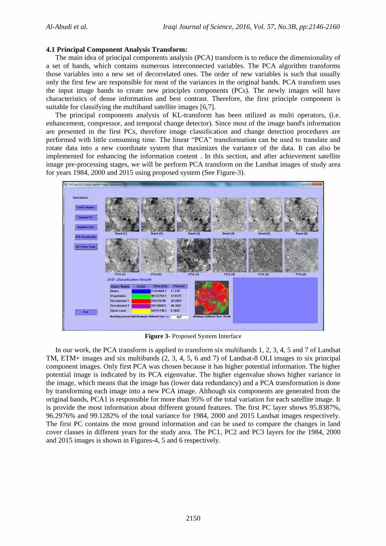
implemented for enhancing the information content . In this section, and after achievement satellite

image pre-processing stages, we will be perform PCA transform on the Landsat images of study area

for years 1984, 2000 and 2015 using proposed system (See Figure-3).

Figure 3- Proposed System Interface

In our work, the PCA transform is applied to transform six multibands 1, 2, 3, 4, 5 and 7 of Landsat

TM, ETM+ images and six multibands (2, 3, 4, 5, 6 and 7) of Landsat-8 OLI images to six principal

component images. Only first PCA was chosen because it has higher potential information. The higher

potential image is indicated by its PCA eigenvalue. The higher eigenvalue shows higher variance in

the image, which means that the image has (lower data redundancy) and a PCA transformation is done

by transforming each image into a new PCA image. Although six components are generated from the

original bands, PCA1 is responsible for more than 95% of the total variation for each satellite image. It

is provide the most information about different ground features. The first PC layer shows 95.8387%,

96.2976% and 99.1282% of the total variance for 1984, 2000 and 2015 Landsat images respectively.

The first PC contains the most ground information and can be used to compare the changes in land

cover classes in different years for the study area. The PC1, PC2 and PC3 layers for the 1984, 2000

and 2015 images is shown in Figures-4, 5 and 6 respectively.


2151

Figure 4- Results of PCA Transform Generated from Bands of Landsat-5 (TM)

Satellite Images for Baghdad City (27/8/1984)

Figure 5- Results of PCA Transform Generated from Bands of Landsat-7 (ETM+)


Figure 6- Results of PCA Transform Generated from Bands of Landsat-8 (OLI)


4.2 Satellite Image Segmentation:

One of the most familiar partition techniques is the quad tree method, which subdivides a region of

an image into four equal blocks when a given homogeneity criterion is not met by that region. It

continues to divide each sub-division until the criteria is met or minimum block size is reached.

Typically, an image is initially divided into a set of large blocks (their size equal to the maximum

allowable block size). The variance is computed and compared to a threshold for each of these blocks.

Any sub-blocks created by failure of the homogeneity test undergo the same procedure. The

subdivision will continue until a block either reaches a minimum size or it satisfies the homogeneity

criterion. Each block test constitutes a node of the quad tree. A node for which no further subdivision

is needed is called a leaf [8]. In this work, a quad tree algorithm is proposed; it is based on the image

uniformity criterion. In this section, we applied quad tree algorithm to partition the first principle

component (PCA 1) image for years 1984, 2000 and 2015 into sub regions represents the area of

study. The efficiency of such method is due to its ability to effectively partitioning diversity regions in


2152

the satellite image. Satellite image segmentation algorithm can be given in algorithm (1) as the

following [8]:

Algorithm (1): Satellite Image Segmentation using Quad tree Algorithm

Input:

PcImg: first PCA image band

Wdth: width of the first PC image

Hght: height of the first PC image

Output:

Llist: One-dimensional array represents grid of quad tree partitioning

Procedure:

Step 1:Compute the global mean (M) and the standard deviation ( ) of the whole input (initial)

image, this factor will be used to automatically determine the threshold value of the dispersion

level (in the uniformity criterion).

Step 2: Set the values of some partitioning control parameters, which can be considered as attributes

of the partitioning process, these parameters are the:

A. Maximum block size (Smax): represent the maximum size of the block corresponds to the

minimum depth of the tree partitioning.

B. Minimum block size (Smin): represent the minimum size of the block corresponds to the

maximum depth of the tree partitioning.

C. Inclusion factor ( ): represent the multiple factor, when it is multiplied by the global

standard deviation ( ) it will define the value of the extended standard deviation ( e ),

i.e. e .

D. Acceptance Ratio (R): represent the ratio of the number of pixels whose values differ from

the block mean by a distance more than the expected extended standard deviation.

Step 3:In order to store information about quad tree partitioning process, quad tree link list was

utilized, it is defined as an array of records, each record of type quad tree link list consist of

the following parameters:

i. Position: represented by the X and Y coordinates of the upper left corner of each block

ii. Size: represent the size of each image block, which is equal either to width or height of

the image block, since in quad tree the blocks have square shape

iii. Next: it is a pointer to the next block in the quad tree

Step 4: The segmentation process by quad tree algorithm start with partitioning the image into blocks

whose size is equal to the maximum allowable block size.

Step 5: Check the uniformity criteria for each sub-block as follows:

A. Compute the local mean of the sub-block (m).

B. Compute number of undesired pixels within the sub-block (NP), which may differ from the

absolute value of mean (m) and pixel value f (x, y) by a distance more than ( e ), those

pixels satisfy the condition

e),( myxf , Where, ),( yxf is the pixel value.

C. If the ratio of undesired pixels (NP/S), where S is the block size, is less than the acceptance

ratio then the block is considered uniform (i.e., don’t partition), otherwise the block should

be partitioned into four child sub-blocks (corresponding to create new four quad tree link

list records). Each block should be examined by measuring its uniformity if it does not

satisfy the uniformity criteria, then the partitioning is repeated until the uniformity

condition is satisfied or the child block reach the minimum size. After completing the

partitioning sequence, the constructed quad tree will consist of partitions whose size value

will be between the minimum and maximum block size.

Figure-7 show the segmentation results using quad tree algorithm of the PCA1 image with different

segmentation control parameters for Landsat-5 TM (27/8/1984) satellite image. It is observed that the

sizes of the image blocks are variable. In all parts, the block size was automatically determined

according to the details variety. The testing results had indicated that the used algorithm is a simple

and powerful framework for the quad tree segmentation. The control parameters have different

influence on the segmentation results. In our work, the best results were obtained when the control


2153

parameters as the following: maximum block size=8, minimum block size=4, inclusion factor =0.5,

acceptance ratio=0.1 and mean factor=0.05.

Maximum Block Size=32

Minimum Block Size=16

Inclusion Factor =0.5

Acceptance Ratio=0.1

Mean Factor=0.05





Mean Factor=0.05





Mean Factor=0.05



Inclusion Factor =1


Mean Factor=0.7



Inclusion Factor =1


Mean Factor=0.1



Inclusion Factor =1


Mean Factor=0.3

Figure 7- Results of quad tree segmentation applied on the PCA- 1 image generated from Landsat-5 (TM)

satellite image (27/8/1984) with different partitioning control parameters

4.3 Supervised Classification using SVD Algorithm:

Singular Value Decomposition (SVD) is a powerful tool in multispectral image analysis. The SVD

of a matrix can be directly used for noise reduction, data compression, and dimension reduction. In

addition, it is also related to the processes of classification. Latent semantic analysis is a vector space

model for index and retrieval of information technology, this method mainly uses singular value

decomposition (SVD) and reduces dimension as the basis of the theory of modules to find implicit

concept in document. Some of the latent semantic analysis researches are used in text or web pages.

SVD is a decomposition technology and uses the singular value decomposition to reduce the size of

the high-dimensional matrix. Through dimension reduced, can extracted important information in the

semantic space. After the decomposition, new matrix and original matrix of the features are similar

and new matrix can more accurately describe the matrix of the hidden semantic concept [9-11].

In our work, we adopt singular value decomposition to selected important semantic features in

scenes and classify the satellite image. Singular value decomposition (SVD) is proposed to perform

supervised classification for partitioned PC1 image, it is consists of two phases: the training and

classification. The training phase is responsible on storing the classes in the database file. The training

area consists of five land cover classes (water, vegetation, open land, residential I and residential II),


2154

training area are collected from all parts of the study area. While the task of classification phase is to

compute the similarity measure between the SVD of the target image and SVD of the classes, found in

the database. Satellite image classification algorithm using SVD can be given in algorithm (2) as the

following:

Algorithm (2): Satellite Image Classification using SVD Algorithm

Input:

PC Img: two-dimensional array is the first pc image

A: 2D array represents the training data from image and vector q that represent the block from image

embedded with A

m: the row dimension of A

n: the column dimension of A

Output:

U: an m-by-n orthogonal matrix represents the left singular value

V: an n-by-n orthogonal matrix represents the right singular value

S: an n-by-n diagonal matrix represents the left singular value

ClasImg: two-dimensional array represents the colored map of classification results

Procedure:

Step 1: Takes an mxn matrix a and decomposes it into uwv, where u,v are left and right orthogonal

transformation matrices, and d is a diagonal matrix of singular values

Step 2: Input to svd is as follows:

i. a = mxn matrix to be decomposed, gets overwritten with u

ii. m = row dimension of a

iii. n = column dimension of a

iv. w = returns the vector of singular values of a

v. v = returns the right orthogonal transformation matrix.

Step 3: Apply Householder reduction to bidiagonal form to the left-hand reduction and to the right-

hand reduction.

Step 4: Accumulate the right-hand transformation.

Step 5: Accumulate the left-hand transformation.

Step 6: Diagonalization of the bidiagonal form (Loop over singular value and over allowed iterations).

Step 9: Find the convergence by making singular value non-negative.

Step 10: Apply Shift from bottom 2 x 2 minor and compute the next QR transformation.

Step 11: Apply arbitrary rotation if singular value equal to zero.

Step 12: return v and w.

Step 14: Assign a specific color for each label, and draw the image (ClasImg) with the new coloring,

which is the classified image.

In this method Landsat images at different time classified into five classes. These classes represent

five major features in the study area (water, open land, vegetation, residential land I and residential

land II). The results from applying singular value decomposition classification algorithm are shown in

Figure-8 for Landsat (TM, ETM+ and OLI) satellite images. Table-1 shows the results of supervised

classification statistics for all three years 1984, 2000 and 2015 using SVD algorithm.


2155

Figure 8- Results of supervised classification using singular value decomposition (SVD) algorithm

(A) Landsat- 5 (TM) satellite image (27/8/1984), (B) Landsat- 7 (ETM+) satellite image (31/8/2000)

(C) Landsat- 8 (OLI) satellite image (1/8/2015)

Table 1- Results of supervised classification statistics for all three Landsat satellite images using SVD algorithm

CLASS

NAME

CLASS

COLOR

Landsat-5 TM (1984) Landsat-7 ETM+ (2000) Landsat-8 OLI (2015)

Area

(KM2)

Percent

%

Area

(KM2)

Percent

%

Area

(KM2)

Percent

%

Water Blue 13.166586 1.8629 14.6677846 2.0753 20.1940896 2.8572

Vegetation Green 70.4906036 9.9735 142.978565 20.2296 131.733004 18.6385

Residential I Red 256.95516 36.3558 249.213103 35.2604 288.739718 40.8529

Residential II Magenta 317.922623 44.9819 199.812078 28.2708 186.534527 26.3922

Open Land Yellow 48.244027 6.8259 100.107471 14.1639 79.5776612 11.2592

Total 706.7789996 100% 706.7790016 100% 706.7789998 100%

5. Satellite Image Classification using Envi 5.1 Software:

The methodology adopted for this stage including different image techniques; geometric correction,

radiometric correction, atmospheric correction, false color composite (bands 4, 3 and 2) and image

enhancement. Supervised classification was used in satellite image classification process. The

algorithm used in supervised classification was the maximum likelihood classifier method to produce

the land cover maps from Landsat TM, ETM+, and OLI satellite images for years 1984, 2000 and

2015. The block diagram of the methodology is shown in Figure-9.

Legend

Water

Vegetation

Residential I

Residential II

Open Land


2156

Figure 9- Block Diagram of Methodology Using ENVI 5.1 Software

The training area collected from all imageries by selecting the region of interest (ROIs) using Envi

software, the study area classified into five classes (residential I, residential II, vegetation, open land

and water bodies). therefore, five ROIs were collected for Landsat images. Figure-10 shows the results

of supervised classification for Landsat (TM, ETM+ and OLI) satellite images using maximum

likelihood classifier method. The image classification of the study area resulted into five land cover

types. Table-2 show the results of supervised classification statistics for all three years (1984, 2000

and 2015) using maximum likelihood classifier method.

Input Satellite Images

Satellite Image Pre-processing

Band Selection for Color Composite

(False Color Composite) bands 4, 3, 2

Contrast-Stretching Enhancement

Supervised Classification

Training area selection

Maximum Liklihood

Classifier Method

Change Detection for Study Area

Output Results


2157

Figure 10- Results of supervised classification using maximum likelihood classifier method

(A) Landsat- 5 (TM) satellite image (27/8/1984), (B) Landsat- 7 (ETM+) satellite image (31/8/2000)

(C) Landsat- 8 (OLI) satellite image (1/8/2015)

Table 2-Results of supervised classification statistics for all three Landsat satellite images using Maximum

Likelihood method

CLASS

NAME

CLASS

COLOR

Landsat-5 TM (1984) Landsat-7 ETM+ (2000) Landsat-8 OLI (2015)

Area

(KM2)

Percent

%

Area

(KM2)

Percent

%

Area

(KM2)

Percent

%

Water Blue 12.636 1.787829 12.4146 1.756504 19.7073 2.788326

Vegetation Green 63.8127 9.028664 134.8038 19.072978 126.2628 17.864538

Residential I Red 251.2566 35.549528 223.5699 31.632222 274.7979 38.880315

Residential II Magenta 335.1609 47.420891 241.6968 34.196941 212.1552 30.017191

Open Land Yellow 43.9128 6.213088 94.2939 13.341356 73.8558 10.449631

Total 706.779 100% 706.779 100% 706.779 100%

6. Land Cover Change Detection:

In our work, monitoring land cover changes was achieved using three Landsat satellite images

taken at different times represented by three dates; 1984, 2000 and 2015. The changes in land cover

occurred in the study area in the period from 1984 to 2015 have been calculated by the subtraction

processes. The results or the changes in land cover are illustrated in Tables-3 and 4 for SVD

classification method. While, Tables 5 and 6 show the results of changes in land cover for maximum

likelihood classifier method. Where the changes are given in square kilometers and in percent. The

type of change (decrease or increase) is also shown.

Table 3-Changes in the Land Cover of the Period from 1984 to 2000 for Baghdad city using SVD Classification

algorithm

CLASS

NAME

Landsat-5 TM (1984) Landsat-7 ETM+ (2000) Relative

Changes

for Area

(KM2)

(2000-

1984)

Relative

Changes

%

Type of

Change

in

Area

Area

(KM2)

Percent

%

Area

(KM2)

Percent

%

Water 13.166586 1.8629% 14.6677846 2.0753% 1.5011986 11.40% increase

Vegetation 70.4906036 9.9735% 142.978565 20.2296% 72.4879614 102.83% increase

Residential I 256.95516 36.3558% 249.213103 35.2604% -7.742057 -3.01% decrease

Residential II 317.922623 44.9819% 199.812078 28.2708% -118.110545 -37.15% decrease

Open Land 48.244027 6.8259% 100.107471 14.1639% 51.863444 107.50% increase

Legend

Water

Vegetation

Residential I

Residential II

Open Land


2158

Table 4-Changes in the Land Cover of the Period from 1984 to 2015 for Baghdad city using SVD Classification

algorithm

CLASS

NAME

Landsat-5 TM (1984) Landsat-8 OLI (2015) Relative

Changes

for Area

(km2)

(2015-

1984)

Relative

Changes

%

Type of

Change

in

Area

Area

(km2)

Percent

%

Area

(km2)

Percent

%

Water 13.166586 1.8629% 20.1940896 2.8572% 7.0275036 53.37 % increase

Vegetation 70.4906036 9.9735% 131.733004 18.6385% 61.2424004 86.88 % increase

Residential I 256.95516 36.3558% 288.739718 40.8529% 31.784558 12.36 % increase

Residential II 317.922623 44.9819% 186.534527 26.3922% -131.388096 -41.32 % decrease

Open Land 48.244027 6.8259% 79.5776612 11.2592% 31.3336342 64.94 % increase

Table 5- Changes in the Land Cover of the Period from 1984 to 2000 for Baghdad city using Maximum

Likelihood Classifier Method

CLASS

NAME

Landsat-5 TM (1984) Landsat-7 ETM+ (2000) Relative

Changes

for Area

(km2)

(2000-

1984)

Relative

Changes

%

Type of

Change

in

Area

Area

(km2)

Percent

%

Area

(km2)

Percent

%

Water 12.636 1.787829% 12.4146 1.756504% -0.2214 -1.75 % decrease


Residential I 251.2566 35.549528% 223.5699 31.632222% -27.6867 -11.01 % decrease

Residential II 335.1609 47.420891% 241.6968 34.196941% -93.4641 -27.88 % decrease


Table 6- Changes in the Land Cover of the Period from 1984 to 2015 for Baghdad city using Maximum

Likelihood Classifier Method

CLASS

NAME

Landsat-5 TM (1984) Landsat-8 OLI (2015) Relative

Changes

for Area

(km2)

(2015-1984)

Relative

Changes

%

Type of

Change

in

Area

Area

(km2)

Percent

%

Area

(km2)

Percent

%

Water 12.636 1.787829% 19.7073 2.788326% 7.0713 55.96 % increase


Residential

I 251.2566 35.549528% 274.7979 38.880315% 23.5413 9.36 % increase

Residential

II 335.1609 47.420891% 212.1552 30.017191% -123.0057 -36.70 % decrease


From classification results using (SVD and maximum likelihood algorithms), the present study

allows estimating the amount of significant land cover changes occurred at the study area during the

two periods. The most significant change for the period 1984-2015 is represented by increasing the

water body, area of vegetation, open land and urban area "residential I" (positive change), while, the

change was negative represented by decrease of urban area "residential II".

The results from applying SVD classification method showed that the water, vegetation area,

residential I and open land are in increase, water increased about 53.37%, vegetation area about

86.88%, "residential I" about 12.36% and finally open land increased about 64.94% in 2015

comparable with 1984, while, the second type from urban area "residential II" in decrease, about

41.32% in 2015 comparable with 1984. The results from applying maximum likelihood classifier

method showed that the water, vegetation area, residential I and open land are in increase, water

increased about 55.96%, vegetation area about 97.86%, "residential I" about 9.36% and finally open

land increased about 68.18% in 2015 comparable with 1984, while, the second type from urban area

"residential II" in decrease, about 36.7% in 2015 comparable with 1984.

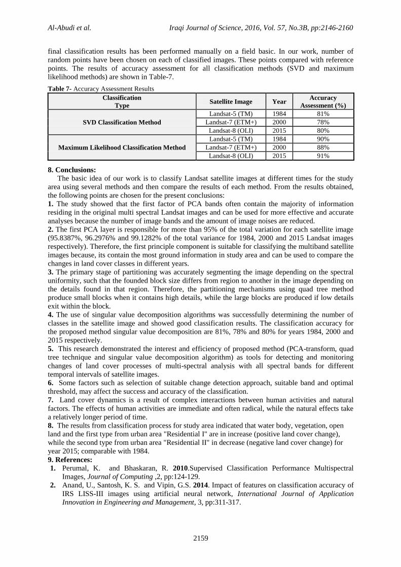
7. Classification Accuracy Assessment:

Accuracy assessment is a procedure for quantifying how good a job was done by a classifier or

how accurate out classification is. Accuracy assessment is an important part of classification. It is

usually done by comparing the classification product with some reference data that is believed to

reflect the true land cover accurately [12]. Sources of reference data include ground truth, higher

spatial resolution images, and maps refer to Google map or Google Earth as needed. Assessing of the


2159

final classification results has been performed manually on a field basic. In our work, number of

random points have been chosen on each of classified images. These points compared with reference

points. The results of accuracy assessment for all classification methods (SVD and maximum

likelihood methods) are shown in Table-7.

Table 7- Accuracy Assessment Results

Classification

Type Satellite Image Year

Accuracy

Assessment (%)

SVD Classification Method

Landsat-5 (TM) 1984 81%

Landsat-7 (ETM+) 2000 78%

Landsat-8 (OLI) 2015 80%

Maximum Likelihood Classification Method

Landsat-5 (TM) 1984 90%

Landsat-7 (ETM+) 2000 88%

Landsat-8 (OLI) 2015 91%

8. Conclusions:

The basic idea of our work is to classify Landsat satellite images at different times for the study

area using several methods and then compare the results of each method. From the results obtained,

the following points are chosen for the present conclusions:

1. The study showed that the first factor of PCA bands often contain the majority of information

residing in the original multi spectral Landsat images and can be used for more effective and accurate

analyses because the number of image bands and the amount of image noises are reduced.

2. The first PCA layer is responsible for more than 95% of the total variation for each satellite image

(95.8387%, 96.2976% and 99.1282% of the total variance for 1984, 2000 and 2015 Landsat images

respectively). Therefore, the first principle component is suitable for classifying the multiband satellite

images because, its contain the most ground information in study area and can be used to compare the

changes in land cover classes in different years.

3. The primary stage of partitioning was accurately segmenting the image depending on the spectral

uniformity, such that the founded block size differs from region to another in the image depending on

the details found in that region. Therefore, the partitioning mechanisms using quad tree method

produce small blocks when it contains high details, while the large blocks are produced if low details

exit within the block.

4. The use of singular value decomposition algorithms was successfully determining the number of

classes in the satellite image and showed good classification results. The classification accuracy for

the proposed method singular value decomposition are 81%, 78% and 80% for years 1984, 2000 and

2015 respectively.

5. This research demonstrated the interest and efficiency of proposed method (PCA-transform, quad

tree technique and singular value decomposition algorithm) as tools for detecting and monitoring

changes of land cover processes of multi-spectral analysis with all spectral bands for different

temporal intervals of satellite images.

6. Some factors such as selection of suitable change detection approach, suitable band and optimal

threshold, may affect the success and accuracy of the classification.

7. Land cover dynamics is a result of complex interactions between human activities and natural

factors. The effects of human activities are immediate and often radical, while the natural effects take

a relatively longer period of time.

8. The results from classification process for study area indicated that water body, vegetation, open

land and the first type from urban area "Residential I" are in increase (positive land cover change),

while the second type from urban area "Residential II" in decrease (negative land cover change) for

year 2015; comparable with 1984.

9. References:

1. Perumal, K. and Bhaskaran, R. 2010.Supervised Classification Performance Multispectral

Images, Journal of Computing ,2, pp:124-129.

2. Anand, U., Santosh, K. S. and Vipin, G.S. 2014. Impact of features on classification accuracy of

IRS LISS-III images using artificial neural network, International Journal of Application

Innovation in Engineering and Management, 3, pp:311-317.


2160

3. Mamdouh, M. Abdeen and Fatima Al Masoudi. Utilization of Multi-Dates and Multi-Sensors

Remote Sensing Data in Monitoring Land Use/Land Cover Changes in Kuwait, Geography

Department, Kuwait University, Alshuwaykh, State of Kuwait.

4. Paul M. Mather, and Magaly, K. 2011.Computer Processing of Remotely-Sensed Images: An

Introduction, Wiley Blackwell, Nottingham, Fourth Edition.

5. M. Anji Reddy. 2008. Textbook of Remote Sensing and Geographical Information Systems, BS

Publications, Third Edition.

6. Ravi P. Gupta, Reet K. Tiwari, Varinder Saini and Neeraj Srivastava. 2013. A Simplified

Approach for Interpreting Principal Component Images. Advances in Remote Sensing, 2, pp:111-

119.

7. Balaji T. and Sumathi M. 2014. PCA Based Classification of Relational and Identical Features of

Remote Sensing Images, International Journal of Engineering and Computer Science, 3(7),

pp:7221-7228.

8. Bushra Qassim Al-Abudi. 2002. Color Image Data Compression Using Multilevel Block

Truncation Coding Technique, Ph.D. Thesis, Baghdad University, College of Science.

9. Chu Hui Lee and Kun-Cheng Chiang. 2010. Latent Semantic Analysis for Classifying Scene

Images, Proceedings of the International Multiconference of Engineers and Computer Scientists,

Hong Kong, 2, pp:17-19.

10. Pavel, P., Libor, M. and Vaclav, S.2004. Iris Recognition Using the SVD-Free Latent Semantic

Indexing", Fifth International Workshop on Multimedia Data Mining, pp:67-70.

11. Bhandari, A. K., Kumar, A. and Padhy, P. K.2011. Enhancement of Low Contrast Satellite

Images using Discrete Cosine Transform and Singular Value Decomposition, World Academy of

Science, Engineering and Technology Journal ,5, pp:20-26.

12. R. G.Congalton, and K. Green. 1999. Assessing the Accuracy of Remotely Sensed Data:

Principles and Practices, Lewis Publishers, Boca Raton.

study of land cover changes of baghdad using multi ... · study of land cover changes of baghdad...

Documents