Study of Flexural Behaviour of Jeffcott Rotor

A Project Report Submitted in the Partial Fulfilment of the Requirements for the Degree of

B. Tech. (Mechanical Engineering)

By SURAJ KUMAR DAS Roll No. 109ME0367

Under the supervision of Dr.H.P.ROY

Assistant Professor Department of Mechanical Engineering, NIT, Rourkela

Department of Mechanical Engineering

C E R T I F I C A T E This is to certify that the work in this thesis entitled Study of Flexural Behaviour of Jeffcott Rotor by Suraj Kumar Das, has been carried out under my supervision in partial fulfilment of the requirements for the degree of Bachelor of Technology in Mechanical Engineering during session 2012 - 2013 in the Department of Mechanical Engineering, National Institute of Technology, Rourkela. To the best of my knowledge, this work has not been submitted to any other University/Institute for the award of any degree or diploma.

Dr. H.P Roy (Supervisor)

Assistant Professor Dept. of Mechanical Engineering National Institute of Technology

Rourkela - 769008

ACKNOWLEDGEMENT

I would like to express my deep sense of gratitude and respect to my

supervisor Prof. H.P Roy for his excellent guidance, suggestions and

support. I consider myself extremely lucky to be able to work under the

guidance of such a dynamic personality. I am also thankful to Prof. K.P

Maity, H.O.D, Department of Mechanical Engineering, N.I.T., Rourkela for

his constant support and encouragement.

Last but not the least, I extend my sincere thanks to all other faculty

members and my friends at the Department of Mechanical Engineering,

NIT, Rourkela, for their help and valuable advice in every stage for

successful completion of this project report.

SURAJ KUMAR DAS Roll No. 109ME0367 Mechanical Engineering Department NIT ROURKELA

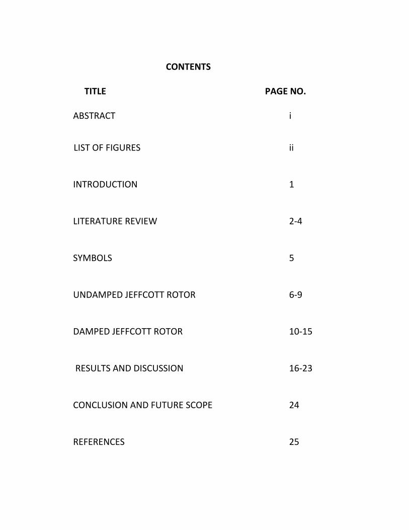
CONTENTS

TITLE PAGE NO. ABSTRACT i

LIST OF FIGURES ii INTRODUCTION 1 LITERATURE REVIEW 2-4 SYMBOLS 5 UNDAMPED JEFFCOTT ROTOR 6-9 DAMPED JEFFCOTT ROTOR 10-15 RESULTS AND DISCUSSION 16-23 CONCLUSION AND FUTURE SCOPE 24 REFERENCES 25

i

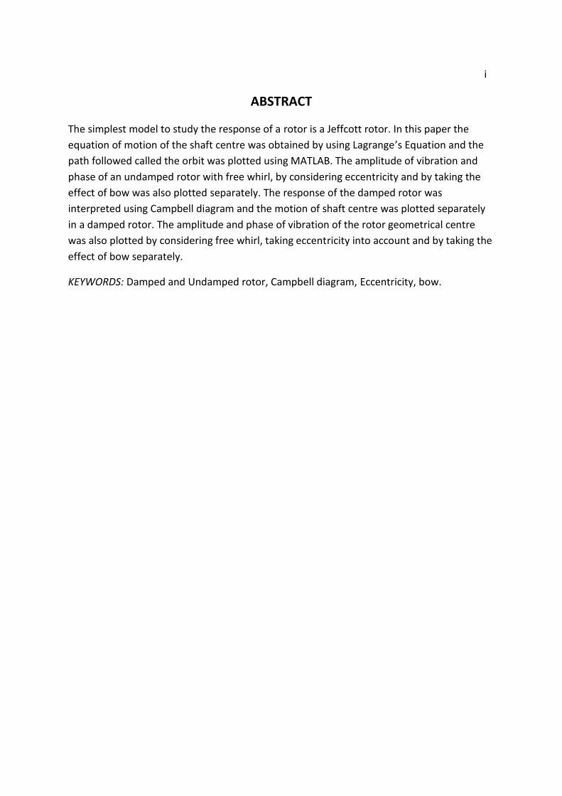
ABSTRACT

The simplest model to study the response of a rotor is a Jeffcott rotor. In this paper the

equation of motion of the shaft centre was obtained by using Lagrange’s Equation and the

path followed called the orbit was plotted using MATLAB. The amplitude of vibration and

phase of an undamped rotor with free whirl, by considering eccentricity and by taking the

effect of bow was also plotted separately. The response of the damped rotor was

interpreted using Campbell diagram and the motion of shaft centre was plotted separately

in a damped rotor. The amplitude and phase of vibration of the rotor geometrical centre

was also plotted by considering free whirl, taking eccentricity into account and by taking the

effect of bow separately.

KEYWORDS: Damped and Undamped rotor, Campbell diagram, Eccentricity, bow.

ii

LIST OF FIGURES

Figure name Figure No./ Page No.

1. Set up of an undamped Jeffcott rotor 1/6

2. Set up of a damped Jeffcott rotor 2/10

3. Representation of xc(t) vs t of undamped rotor 3/16

4. . Representation of yc(t) vs t of undamped rotor 4/17

5. Orbit of point C of undamped rotor 5/17

6. Unbalance response of amplitude of

Undamped Jeffcott rotor 6/18

7. Non dimensional response of undamped

Jeffcott rotor to shaft bow 7/18

8. Decay rate plot of a damped Jeffcott rotor 8/19

9. Campbell Diagram 9/20

10. Unbalance response of a damped Jeffcott rotor

non – dimensional amplitude 10/20

11. Unbalance response of a damped Jeffcott rotor

non – dimensional phase 11/21

12. Non-dimensional trajectories of point P and C

In the rotating plane O ζ η 12/21

13. Response of damped Jeffcott rotor to shaft bow

Non- dimensional amplitude vs non dimensional spin 13/22

14. Response of damped Jeffcott rotor to shaft bow

Non- dimensional phase vs non dimensional spin 14/23

1

INTRODUCTION

Jeffcott rotor is the simplest model to study the flexural behaviour of rotor mass system. In

this model the rotor was assumed to be massless and a point mass is attached to the rotor

at some distance from the centre called eccentricity. The Jeffcott rotor is also referred to as

De Laval rotor. The response of rotor deviates accordingly to various physical conditions.

The speed of the rotor when match with the natural frequency then it is called critical

speed. The speed of rotor below critical speed is called sub-critical speed and the speed

above critical speed is called super-critical speed. In a damped rotor the direction of whirl

determines the stability of the system. If the whirl speed is same as that of the shaft speed

called (forward whirl) then rotor is stable in sub- critical range and in super- critical region

depends on different parameters. On the other hand if the whirl speed is opposite to

angular speed then the system becomes stable. The response is clearly understood by

Campbell Diagram. The rotor is modelled by considering both damping and undamped

condition.

Although Jeffcott rotor is the more idealized model as compared to real life rotors used in

steam turbine, jet planes, IC engine shaft etc. it retains some basic characteristics and allows

us to gain a qualitative insight into important phenomena of rotor dynamics.

2

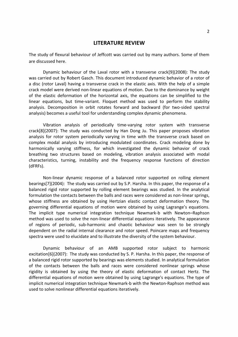
LITERATURE REVIEW

The study of flexural behaviour of Jeffcott was carried out by many authors. Some of them

are discussed here.

Dynamic behaviour of the Laval rotor with a transverse crack[9](2008): The study was carried out by Robert Gasch. This document introduced dynamic behavior of a rotor of a disc (rotor Laval) having a transverse crack in the elastic axis. With the help of a simple crack model were derived non-linear equations of motion. Due to the dominance by weight of the elastic deformation of the horizontal axis, the equations can be simplified to the linear equations, but time-variant. Floquet method was used to perform the stability analysis. Decomposition in orbit rotates forward and backward (for two-sided spectral analysis) becomes a useful tool for understanding complex dynamic phenomena.

Vibration analysis of periodically time-varying rotor system with transverse crack[8](2007): The study was conducted by Han Dong Ju. This paper proposes vibration analysis for rotor system periodically varying in time with the transverse crack based on complex modal analysis by introducing modulated coordinates. Crack modeling done by harmonically varying stiffness, for which investigated the dynamic behavior of crack breathing two structures based on modeling, vibration analysis associated with modal characteristics, turning, instability and the frequency response functions of direction (dFRFs).

Non-linear dynamic response of a balanced rotor supported on rolling element bearings[7](2004): The study was carried out by S.P. Harsha. In this paper, the response of a balanced rigid rotor supported by rolling element bearings was studied. In the analytical formulation the contacts between the balls and races were considered as non-linear springs, whose stiffness are obtained by using Hertzian elastic contact deformation theory. The governing differential equations of motion were obtained by using Lagrange’s equations. The implicit type numerical integration technique Newmark-b with Newton–Raphson method was used to solve the non-linear differential equations iteratively. The appearance of regions of periodic, sub-harmonic and chaotic behaviour was seen to be strongly dependent on the radial internal clearance and rotor speed. Poincare maps and frequency spectra were used to elucidate and to illustrate the diversity of the system behaviour. Dynamic behaviour of an AMB supported rotor subject to harmonic excitation[6](2007): The study was conducted by S. P. Harsha. In this paper, the response of a balanced rigid rotor supported by bearings was elements studied. In analytical formulation of the contacts between the balls and races were considered nonlinear springs whose rigidity is obtained by using the theory of elastic deformation of contact Hertz. The differential equations of motion were obtained by using Lagrange's equations. The type of implicit numerical integration technique Newmark-b with the Newton-Raphson method was used to solve nonlinear differential equations iteratively.

3 The appearance of the regions of periodic behavior, sub-harmonic and chaotic it is heavily dependent on radial and rotor speed. Poincaré maps and frequency spectra were used to elucidate and to illustrate the diversity of the system behavior. Non-linear coupled dynamics of flexible blade–rotor–bearing systems [5](2009): The study was carried out by Ligang Wang, D.Q.Cao, Wenhu Huang. In this paper, the nonlinear dynamic behavior of a rotor system supporting interaction between the blades and rotor. Using Lagrange's equation was established nonlinear model of a time-dependent system rotor blade-bearing flexible, in which the rotor is supported by the journal bearings and blades is modeled as pendulums to analyze dynamic coupling between the elastic laminar and flexible shaft. To emphasize the gyroscopic effect of the rotor, it is assumed that the disk is located at an arbitrary position of the shaft. The use of orthogonal transformations, Equations 1 nodal diameter blade movement, which engage with the equations of the dynamics of the rotor are uncoupled with other equations of the blades. Then the parametric excitation terms in the system of the rotor blade support is simplified in terms of periodic transformations. The dynamic equations along with the forces of nonlinear oil film were solved numerically using the Runge-Kutta method. Bifurcation diagrams, three-dimensional spectral plots and Poincaré maps' were used to analyze the dynamic behavior of the system. Theoretical analysis of the non-linear behaviour of a flexible rotor supported by herringbone grooved gas journal bearings[4](2006): The study was conducted by Cheng-Chi Wanga, Her-Terng Yaub, Ming-Jyi Jangc, Yen-Liang Yeh. In this work we studied the behavior of a flexible rotor supported by a publishing system that carries gas slotted pin. The finite difference method is used for successive relaxation technique to solve the Reynolds equation. The state system trajectories, Poincaré maps ofpower spectra and bifurcation diagrams are used to analyze the dynamic behavior of the rotor and the center of the magazine in the horizontal and vertical directions at different operating conditions. The analysis revealed a complex dynamic behavior comprising periodic responses and quasi-periodic rotor and the center of the bearing. Non-linear dynamic analysis of dual flexible rotors supported by long journal bearings[3](2010): The study was conducted by Jian Cai-Wan Chang. In this paper, the vibration characteristics of two rotors equipped with long smooth bearings on both ends were investigated. Besides the nonlinear forces lubricated pairs a nonlinear elastic, damped coupling was assumed between the bearings and rotor pedestal. Rotation speed is used as the control parameter for observing various forms of periodic vibrations, quasi-periodic and chaotic. Different cross section and length of the axes, the mass of the bearings and even bearings are different approaches to analyze and discuss the difference in dynamic responses. Dynamic trajectories, Poincaré maps, bifurcation diagrams were used to analyze the behavior of the bearing center in the horizontal and vertical directions under different operating conditions.

4 A fuzzy approach for the analysis of unbalanced nonlinear rotor systems[2](2005): The study was carried out by Yazhao Qiu, Singiresu S. Rao. Most components of the structural and mechanical systems or uncertainties considerable variation in their properties. Therefore, the performance characteristics of such systems are also subject to uncertainties. In the case of a rotor-bearing system, the restoring force of the bearing is usually represented nonlinear as third or fourth power shift or a piecewise linear function of displacement. The coefficients of these models are acquired from experiments and approximations, and can vary considerably during operation of the bearing. Therefore, it is reasonable to treat as uncertain values. Other parameters of support, such as the inertial properties of concentrated disks, distributed mass and damping of the rotating assemblies are also uncertain due to manufacturing and assembly errors and inaccurate operating conditions. It is known that the response to the vibration of a rotor is very sensitive to small changes or variations in the parameters of the bearing. Thus, any analysis and design of rotor bearing systems should take into account realistic uncertainties. In this paper, a methodology for fuzzy analysis of rotor-bearing systems with nonlinear numerical results to demonstrate the computational feasibility of the method. On the non-linear dynamic behaviour of a rotor–bearing system[1](2004): The study was carried out by JingJianPing , MengGuang ,Sun Yi, Xia SongBo. Non-linear dynamic behavior of a rotor-bearing system is analyzed on the basis of a continuum model. The finite element method is adopted in the analyzes. Emphasis is placed on the so-called oil whip phenomena'''', which could lead to failure of the rotor system. The dynamic response of the system in a state of imbalance is addressed by the method of direct integration and mode superposition method. Found that a typical oil whip'''' phenomenon occurs successfully. Moreover, we analyze the behavior of fork oil whip phenomenon is very concerned about the current nonlinear dynamics. The rotor-bearing system is also tested by the simple discrete model. Significant differences were found between these two models. It is suggested that careful consideration must be made in such modeling nonlinear dynamic behavior of rotor system.

5

SYMBOLS

xp(t)- X coordinate of point mass

yp(t)- Y coordinate of point mass

xc(t)- X coordinate of rotor centre

yc(t)- Y coordinate of rotor centre

m- Mass of point mass

ω- Angular velocity of rotor

ωw- Whirl speed of rotor

ωn- Natural frequency of rotor

ωcr- Critical speed of the rotor

k- Stiffness of rotor

x’p(t), x”p(t)- Velocity and acceleration in X direction of point mass

y’p(t), y”p(t)- Velocity and acceleration in Y direction of point mass

x’c(t), x”c(t) - Velocity and acceleration in X direction of rotor centre

y’c(t), y”c(t) - Velocity and acceleration in Y direction of rotor centre

rp- Position of point mass in complex form

r’p, r”p – Velocity and acceleration of point mass in complex form

rc- Position of rotor centre in complex form

r’c, r”c - Velocity and acceleration of rotor centre in complex form

K- Kinetic Energy of point mass

U- Potential Energy stored in the rotor due to rotation

b- rotor bow length

α- Angle of bow w.r.t eccentricity

cn- Non-rotating damping coefficient

cr- Rotating damping coefficient

6

1. UNDAMPED JEFFCOTT ROTOR

Figure 1: Set up of an undamped Jeffcott rotor

1.1 Development of Equation of motion

Consider a Jeffcott rotor rotating at angular speed ω with eccentricity e as shown in the

above figure. Let the point mass be at P and the geometrical rotor centre is at C. Let us

assume that the P always lies on the XY plane. Consider the instant at time t. Position P at

time t is given by,

xp(t)= xc(t)+ecos(ωt) (1.1a)

yp(t)= yc(t)+esin(ωt) (1.1b)

Velocity of P at time t is obtained by taking derivative of equations (1.1a,1.1b),

x’p(t)= x’c(t)-eωsin(ωt) (1.1c)

y’p(t)= y’c(t)+eωcos(ωt) (1.1d)

The Kinetic Energy of mass is,

K= ½*m(x’p2+ y’p

2)

=>K= ½*m((x’c(t)-eωsin(ωt))2+( y’c(t)+eωcos(ωt))2) (1.1e)

And Potential Energy is ,

7

U= ½*k((xc(t))2+( yc(t))2) (1.1f)

Now Lagarnge equation can be written as

(

)

Where qi are the Lagrangian coordinates (xc,yc)

Substituting the values and solving we get, the equation of motion of C is,

m x”c(t) +k xc(t)= me ω2cos(ωt)+Fx(t) (1.1g)

m y”c(t) +kyc(t)= me ω2sin(ωt) +Fy(t) (1.1h)

where Fy(t), Fx(t) are unbalance forces in Xand Y direction respectively.

Again proceeding in the similarly and applying Lagrange’s equation of motion of P is

m x”p(t) +k xp(t)= kecos(ωt)+Fx(t) (1.1i)

m y”p(t) +kyp(t)= kesin(ωt) +Fy(t) (1.1j)

In complex form the equation of motion of point C is given by,

m r”c(t) +k rc(t)= me ω2eiωt+Fn(t) (1.1l)

and the motion of point P is given by,

m r”p(t) +krp(t)= keeiωt +Fn(t) (1.1m)

1.2 Free whirling

In free whirling the effect of unbalance (due to eccentricity) is neglected and there is no

external force on the system. So the equation of motion of C becomes,

m x”c(t) +k xc(t)= 0 (1.2a)

Let the solution of equation be xc(t)= Xcoest where s ϵ C.

8

Substituting the above value of derivatives in equation (1.2.a) we get,

(ms2+k)Xcoest=0 (1.2b)

Since Xcoest≠0,

ms2+k=0. (1.2c)

The absolute value of s becomes, s= ωn=√ , the solution is

xc(t) = X1eist + X2e-ist (1.2d)

yc(t) = Y1eist + Y2e-ist (1.2e)

Where constants X1,2&Y1,2 are obtained from initial conditions.

xc(0)= X1+X2; x’c(0)=i(X1-X2) ωn

yc(0)= Y1+ Y2; y’c(0)=i(Y1- Y2) ωn

Substituting the above values in equation (1.2.c,1.2.d) we get,

xc(t) = xc(0)eist +

e-ist (1.2f)

Similarly,

yc(t) = xc(0)eist +

e-ist (1.2g)

1.3 Unbalance Response

In this section we consider the response of undamped Jeffcott rotor when we take the eccentricity into account. In this case the equation (1h) becomes,

m x”c(t) +k xc(t)= me ω2cos(ωt) (1.3a)

Let the solution is xc(t)= Xcocos(ωt)

Performing similar operation as in equation (1.2a)and substituting the values of derivatives in equation (1.3a), we get,

(k-mω2) Xco= me ω2 (1.3b)

Similarly,

9

(k-mω2) Yco= me ω2 (1.3c)

which gives

Yco= Xco=

=

(

)

(

) (1.3d)

1.4 Shaft bow

Consider a Jeffcott rotor with initial bow. Let the bow makes an angle with the eccentricity and let the bow length be b. Now when we take bow into account then the equation of motion of point C becomes,

m r”c(t) +k rc(t)= me ω2eiωt+ kbei(ωt+α)+Fn(t) (1.4a)

The particular solution of the equation containing only the term linked with the shaft bow is

rc= b*

(1.4b)

| rco |/b=

(1.4c)

10

2.JEFFCOTT ROTOR WITH VISCOUS DAMPING

There are 2 types of damping effect exist in a damped rotor. They are:

Non-rotating damping – Damping that is directly associated stationary part of the rotor. This type of damping has a stabilizing effect and tends to reduce the amplitude of vibration.

Rotating damping – Damping that is directly associated with rotor is called rotating damping. This reduces amplitude of vibration in sub critical conditions but shows destabilizing effect in super critical range.

2.1 Modelling of equation of motion

Consider the rotor mass system as shown in the figure below:

Figure 2: Set up of a damped Jeffcott rotor

The force caused by non-rotating viscous damping is proportional to the speed of the point C in a rotating frame of reference.

So,

Fnxy= (

) = -cn(

) (2.1a)

The force caused rotating viscous damping is proportional to the speed of point C as observed from a frame of reference rotating with the same speed of the rotor. Let the rotating axes are ζ and η. If the angular speed is constant the angle between 2 frames of

11

reference is given by θ= ωt. So the force as observed from the rotating frame of reference is given by:

Frζη= (

) = -cr(

) (2.1b)

The coordinates of ζc, ηc can be expressed in the XY axes as follows:

( ) = R(

) (2.1c)

where R is the rotation matrix given by

R= (

) (2.1d)

By further simplification the force caused by rotating damping in inertial frame of reference is given by,

Frxy= -cr(

) –cr*ω(

)*( ) (2.1e)

Hence the net force on the rotor is given by,

(

)*(

) +(

)*(

) + (*

+ (

))*( ) =

(

) + (

) (2.1f)

The presence of damping gives skew symmetric term in the stiffness matrix i.e to a circulatory matrix. The circulatory matrix vanishes when ω tends to 0. When the spin speed vanishes the rotor becomes a stationary system and it behaves like a natural system.

In complex form the following is obtained,

m r”c+(cr+cn)*r’c+(k-i ωcr)*rc= me ω2eiwt +Fn (2.1g)

12

2.2 Free whirling

In free whirling the effect due to eccentricity an external force is neglected. So the equation of motion becomes,

m r”c+(cr+cn)*r’c+(k-i ωcr)*rc=0 (2.2a)

Let the solution of the homogenous equation be rc= rcoest where rco,s ϵ C

substituting the value of r’’c and r’c , we get,

ms2+( cr+cn)s+( k-i ωcr) =0 (2.2b)

the roots of the above quadratic equation with complex coordinates are

s= σ+i ω=

± √

(2.2c)

Separating the real and imaginary parts we get,

σ 1,2 =

±

√√ (

)

(2.2d)

ωw1,2 = ±

√√ (

)

(2.2e)

where =

-

.

Two solution of the equation (2.2b) can be found for each value of spin speed . Therefore the generalised solution of equation (2.2b) is given by

rc= R1 + R2 (2.2f)

where R1 and R2 can be obtained from initial conditions.

13

Because of non - zero value of σ the motion of point C has an amplitude varying exponentially with time.

If σ is negative the amplitude decays with time and point C tends to point O and rotor has a stable behaviour because the whirl motion tends to reduce the amplitude.

On the other hand if σ is positive the amplitude grows exponentially and the motion is unstable.

2.2.1 Campbell diagram

The equation (2.2d) and (2.2e) can be written in the non-dimensional form as

σ *= -( ζr+ζn) ± √√ * (2.2.1a)

ωw*= √√ * (2.2.1b)

where,

ωw*= ωw/ ωcr , σ *= σ/ ωcr

ω^= ω/ ωcr , *=[1-( ζr+ζn)2]/2 (2.2.1c)

ζr= cr/2 ζn= cn/2

The plot of ωw* vs is called Campbell Diagram.

2.3 Unbalance response

If the eccentricity of the rotor is e then the equation of motion of point C when there is no external force is given by,

m r”c+(cr+cn)*r’c+(k-i ωcr)*rc= me ω2eiωt (2.3a)

14

Let the solution of the equation be rc=rcoeiωt. (rcoϵ C)

Substituting the value of r’c and r”c , we get,

rco(-mω2+iωcn+k)= me ω2 (2.3b)

{assuming no damping due to rotation}

rco= me ω2 /(-mω2+iωcn+k) (2.3c)

Since rco is complex so,

| rco|=

√ (2.3d)

And

ϕ=arctan(

) (2.3e)

The amplitude and phase of rco are plotted in non - dimensional form as functions of speed. Different curves are obtained with different values of ζn.

The complex equation 2.3c when plotted directly (using MATLAB) gives the trajectory of point C. The trajectory of point P is obtained by adding to C.

The maximum amplitude occurs at ω^=

√ (from eq. 2.3d) and the corresponding

maximum amplitude

| rco|max=

√ (2.3f)

If damping is low, then neglecting ζn2, | rco|max e/2 ζn.

The value (1/2 ζn) is referrd to as quality factor. It gives the magnitude of the response when the rotor crosses the critical speed.

2.4 Shaft bow

15

Now consider a Jeffcott rotor with initial bow. Let the bow makes an angle with the eccentricity and let the bow length be b. Now when we take bow into account then the equation of motion of point C becomes,

m r”c+(cr+cn)*r’c+(k-i ωcr)*rc= me ω2eiwt + kbei(α+ωt)+Fn (2.4a)

To find the solution, let rc=rcoeiωt

Now substituting the values of r’c and r”c in equation (2.3a), and assuming (cr=0) we have

rco =

(2.4b)

Rearranging and separating the real and imaginary parts we get,

rco/b= *(

) (

)+ (2.4c)

Now the speed at which shaft bow is maximum is given by,

ω ^rmax=√ (2.4d)

and the corresponding peak amplitude is given by,

|rco|/b=

√ . (2.4e)

16

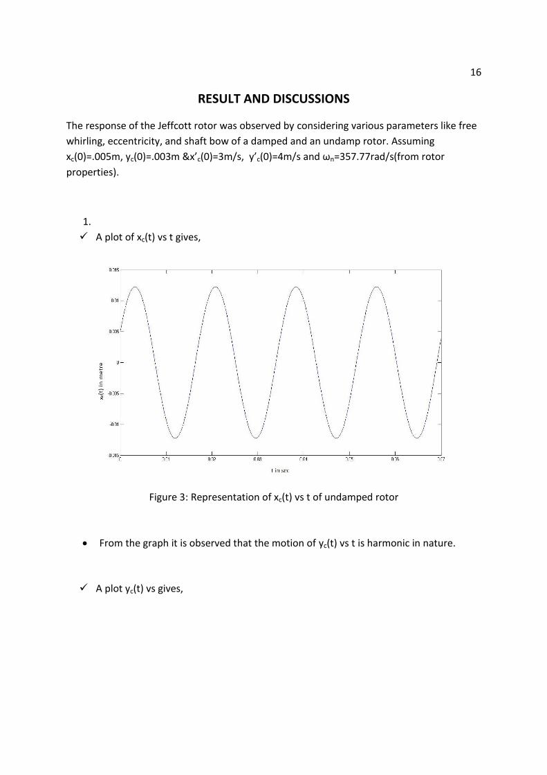
RESULT AND DISCUSSIONS

The response of the Jeffcott rotor was observed by considering various parameters like free

whirling, eccentricity, and shaft bow of a damped and an undamp rotor. Assuming

xc(0)=.005m, yc(0)=.003m &x’c(0)=3m/s, y’c(0)=4m/s and ωn=357.77rad/s(from rotor

properties).

1.

A plot of xc(t) vs t gives,

Figure 3: Representation of xc(t) vs t of undamped rotor

From the graph it is observed that the motion of yc(t) vs t is harmonic in nature.

A plot yc(t) vs gives,

17

Figure 4: Representation of yc(t) vs t of undamped rotor

From the graph it is observed that the motion of yc(t) vs t is harmonic in nature.

Plot of yc(t) vs xc(t) gives,

Figure 5: Orbit of point C of undamped rotor

From the graph it is observed that the plot of yc(t) vs xc(t) gives an ellipse called orbit.

18

2. The plot of Yco/e, Xco/e gives,

Figure 6: Unbalance response of amplitude of Undamped Jeffcott rotor

From the graph it is observed that in the sub-critical rangei.e ω< ωcr , the whirling non- dimensional amplitude increases from 0 to infinity at ωcr.

On the other hand in the super- critical range i.e ω/>ωcr the whirling amplitude is negative and decreases monotonically and when the speed tends to infinity the non- dimensional amplitude tends to (–1).

3.

The plot of | rco |/b vs (ω/ ωcr) is shown,

Figure 7: Non dimensional response of undamped to shaft bow

19

From the graph it is observed that in the sub-critical rangei.e ω< ωcr , the whirling non- dimensional amplitude increases from 1 to infinity at ωcr.

On the other hand in the super- critical range i.e ω/>ωcr the whirling amplitude is negative and decreases monotonically and when the speed tends to infinity the non- dimensional amplitude tends to (–1).

4.

A graph was plot σ * vs ω^ by assuming ζr=ζn and taking 4 values of ζr (0,.1,.2,.3).the following result obtained.

Figure 8: Decay rate plot of a damped Jeffcott rotor

For each value of ζr=ζn we have two types of motion that is forward motion and backward motion because the equation (2.2.1a) has 2 solutions.

The forward motion tends to increase the amplitude and is unstable.

The backward motion tends to decrease the amplitude and is stable

A graph was plot ωw* vs ω^ by assuming ζr=ζn and taking 4 values of ζr (0,.1,.2,.3) the following result obtained. The diagram hence obtained is called Campbell Diagram.

20

Figure 9: Campbell Diagram

From the graph it is observed that when the whirl speed is opposite to the same speed then the corresponding spiral motion is in backward direction and we have stable.

If the whirl speed is same as that of the same spin speed the corresponding spiral motion is in forward direction

5.

Plot of (| rco|/e) vs ω^ gives,

Figure 10: Unbalance response of a damped Jeffcott rotor non – dimensional amplitude

21

The non – dimensional amplitude is 0 when non – dimensional spin speed is zero.

And it tends to 1 when non – dimensional spin speed tends to infinity that is when the rotor operates in a super critical range.

And plot of Φ vs ω^ gives

Figure 11: Unbalance response of a damped Jeffcott rotor of non – dimensional phase

The non –dimensional phase tends to – when the rotor operates in a super critical range and it is equal to /2 when the rotor operates at critical speed.

6.

The point P and C are plotted with ζ/e, η/e as reference axes.

Figure 12: Non-dimensional trajectories of point P and C in the rotating plane O ζ η

22

The trajectory of C as observed from rotating frame of reference that is with ζ η axes is shown by the solid line. The trajectory of P is obtained by adding e to point C, it is shown by dotted line.

Different curves are obtained for different values of ζn. When ζn value is less the radius of spiral of C and P is more, on the other hand when ζn value is more the radius of spiral of C and P is less.

7.

The plot of rco/b vs ω^ gives,

Figure 13: Response of damped Jeffcott rotor to shaft bow non- dimensional amplitude vs non dimensional spin

From graph it is observed that the the amplitude decreases and subsequently vanishes when the rotor operates in a super critical range.

At critical speed the amplitude becomes maximum and tends to infinity.

And plot of ϕ vs ω^ gives,

23

Figure 14: Response of damped Jeffcott rotor to shaft bow non- dimensional phase vs non dimensional spin

The response of the rotor by considering bow along with the phase angle is shown in the graph. The phase angle is /2 at critical speed.

24

CONCLUSION AND FUTURE SCOPE

In an undamped rotor the trajectory of the rotor centre may be circular, rotational or linear,

it depends on the initial condition. Here the natural frequency of the Jeffcott rotor is ωn and

is independent of angular speed. From the amplitude response we observe that the

amplitude tends to infinity at the critical speed or at resonance and decreases

asymptotically when the speed increases that is when the rotor is allowed to operate in

super critical state. In the super critical range, when the spin speed tends to infinity then the

amplitude of point C tends to(- ) or in other words the point P moves towards O. This

phenomenon is called self-centring and is generally favourable.

In a damped rotor the motion of point C as well as P is

spiral. The radius of the spiral decreases with increase in damping coefficient and vice versa.

When the whirl speed is same as spin speed called forward whirl, the rotor is stable in the

sub critical range. On the other hand if the whirl speed is opposite to the spin speed then

the operation is stable and the amplitude decays rapidly.

Though Jeffcott rotor is the ideal rotor and there is

much more modification in the practical rotor but the response of the rotor to various

parameters gives a base for study of real non-ideal rotors. Steps and methods should be

developed to study the actual characteristics of practical used rotor, based on the response

of the Jeffcott rotor.

25

REFERNCE

1. Jing Jian Ping , Meng Guang, Sun Yi, Xia Song Bo, “On the non-linear dynamic behavior of a rotor–bearing system,” Journal of Sound and Vibration, vol. 274, pp. 1031-1044, 2004.

2. Yazhao Qiu, Singiresu S. Rao, “ A fuzzy approach for the analysis of unbalanced nonlinear rotor systems,” Journal of Sound and Vibration, vol. 284, pp. 299-323, 2005.

3. Cai-Wan, Chang-Jian, “Non-linear dynamic analysis of dual flexible rotors supported by long journal bearings,” Mechanism and Machine Theory, vol. 45, pp. 844-866, 2010.

4. Cheng-Chi Wanga, Her-Terng Yau, Ming-Jyi Jang, Yen-Liang Yeh , “Theoretical analysis of the non-linear behaviour of a flexible rotor supported by herringbone grooved gas journal bearings,” Tribology International, vol. 40, pp. 533-541, 2007.

5. Ligang Wang , D.Q.Cao, Wenhu Huang, “Non linear coupled dynamics of flexible blade–rotor–bearing systems,” Tribology International, vol. 43, pp. 759-778, 2010.

6. M.H. Eissa , U.H. Hegazy b, Y.A. Amer, “Dynamic behaviour of an AMB supported rotor subjectto harmonic excitation,” Applied Mathematical Modelling, vol. 32, pp. 1370-1380, 2008.

7. S.P. Harsha, “Non-linear dynamic response of a balanced rotor supported on rolling element bearings,” Mechanical Systems and Signal Processing, vol. 19, pp. 551-578, 2005.

8. Dong Ju Han, “Vibration analysis of periodically time-varyingrotor system with transverse crack,” Mechanical Systems and Signal Processing, vol. 21, pp. 2857-2879, 2007.

9. Robert Gasch, “Dynamic behaviour of the Laval rotor with a transverse crack,” Mechanical Systems and Signal Processing, vol. 22, pp. 790-804, 2008.

10. Giancarlo Genta, “Dynamics of rotating systems,” Springer, pp. 35-68, 2005.