study of effective electrical conductivity of additive ...€¦ · study of effective electrical...
TRANSCRIPT
Journal of Energy and Power Engineering 13 (2019) 249-266
doi: 10.17265/1934-8975/2019.07.001
Study of Effective Electrical Conductivity of Additive
Free Electrodes Using a Homogenization Method
Subash Dhakal1 and Seshasai Srinivasan
1,2
1. Department of Mechanical Engineering, McMaster University, Hamilton, ON L8S 4L8, Canada
2. School of Engineering Practice and Technology, McMaster University, Hamilton, ON L8S 4L8, Canada
Abstract: Conductive additives are used in the cathode of a Li-ion battery to improve electrical conductivity. However, these additives
can negatively impact the ionic conductivity and specific capacity of the battery. Therefore, design of additive-free cathodes is gaining
attention in the research community. In this paper, we explore the effective electrical conductivity of randomly generated two-phase
conductive-free cathode microstructures using a mathematical homogenization method. Over thousand microstructures with various
combinations of particle size, volume fraction and conductivity ratios are considered to evaluate effective electrical conductivity values
using this method. An explicit formulation is proposed based on the results to provide a simple method for evaluation of the effective
conductivity values. The intrinsic properties of each phase of the microstructure are used to obtain the effective electrical conductivity
values. With the microstructure geometry information being utilized for the evaluation of the effective properties, the results obtained
from this formulation are expected to be more accurate and reliable than those obtained using the popular Bruggeman’s approximation,
providing better estimates of discharge characteristics. Finally, the significance of incorporation of micro-structural information to
model cathodes is highlighted by studying the discharge characteristics of Li-ion battery system.
Key words: Lithium ion, additive-free electrode, homogenization, effective conductivity, Bruggeman, particle size.
List of Symbols
σ* Effective conductivity, S/m
σ Intrinsic conductivity, S/m
Volume fraction of conductive phase
j Volume fraction of “j” phase
γ Bruggeman’s exponent
τ Tortuosity
r Domain length normalized particle size
rp/n Actual particle size, μm
N Number of particles
h Conductivity ratio
L Length of domain
Subscripts
AP Active particles
E Electrolyte
p Positive electrode
n Negative electrode
Corresponding author: Seshasai Srinivasan, PhD, Chair,
research fields: software engineering technology, CFD, heat
transfer, lithium batteries.
1. Introduction
With a rapidly increasing population, which is
estimated to be around 7.5 billion by the end of 2017,
the demand for energy is ever increasing. It is estimated
that the energy demand for the world will increase by
48% in 2040 as compared to the demand in 2012 [1].
However, based on the World Energy Council (WEC)
report, only about 14% of the world’s energy demand
was met by renewable energy sources including
hydropower in 2015 [2]. Currently, due to our
over-reliance on the traditional energy sources like coal
and gas to meet this demand, atmospheric carbon
dioxide levels are at an all-time high resulting in global
warming and climate change. Hence, current focus in
the research community is in the development of clean
and renewable energy resources in order to overcome
this problem. Renewable energy systems, including
solar and wind energy, and electric vehicles require
efficient and high-capacity energy storage systems.
Lithium-ion (Li-ion) batteries are the batteries of
D DAVID PUBLISHING
Study of Effective Electrical Conductivity of Additive Free Electrodes Using a Homogenization Method
250
choice in these applications as well as in consumer
electronics such as laptops, cell phones, etc. because
they offer a lot of advantages over other rechargeable
battery systems. Li-ion batteries have very high
specific energy storage capacity, negligible memory
effects and lower self-discharge rate as compared to
other rechargeable battery systems [3].
In order to improve the features such as storage
capacity and rate of discharge of Li-ion batteries,
extensive research has taken place with a focus to
improve the properties of electrodes. Research in this
field involves the improvement of materials used in
electrolytes and electrodes to make them more
cost-competitive and efficient. Typically, a Li-ion
battery consists of the positive and negative electrodes,
electrolyte and a separator. During the charge cycle,
Li-ion is inserted into the negative electrode during
charge and extracted from it during the discharge cycle.
Transfer of Li-ions across the electrodes takes place
simultaneously with the transfer of electrons from the
outer circuit. There are several types of Li-ion batteries
in use in the market currently. The intended application
determines the chemistry, performance and cost
characteristics. Typically, the positive electrode
consists of a Lithium metal oxide (LiFePO4, LiMn2O4,
etc.) and the negative electrode is made up of graphite.
The separator holds these two electrodes apart and is
made up of a permeable membrane. It allows the Li-ion
to pass through it but blocks the flow of electrons hence
avoiding short-circuiting. The electrolyte comprises of
lithium salts (LiPF6, LiBF4, etc.) in an organic solvent
that is typically composed of ethylene carbonate and
dimethyl carbonate (EC: DMC). Positive electrode is
porous with electrolytes residing in pores and is made
up of active particles which are held together by binder
[4, 5].
Additionally, carbon particles are added along
with the binders to increase the overall electronic
conductivity of the cathode of Li-ion batteries.
Although these carbon additives help enhance the
electrical conductivity, they can have a negative effect
on the ionic conductivity. These additives can occupy
anywhere between 10%-40% of the weight of the entire
electrode [6]. However, since these additives are not
directly involved in the electrochemical reactions, they
limit the specific energy capacity of the cell. These
additives create difficulty in modeling of the transport
of Li-ions and electrons. Therefore, it is desirable to
design Li-ion battery cathodes without the inclusion of
these conductive additives. Ha et al. [6] provided a
process for the fabrication of additive-free high
performance cathodes using nanoparticles.
An alternative approach to improve the performance
of a battery without using additives would be to
develop optimally engineered microstructures. It is
well known that one of the key factors affecting the
electrical conductivity is the size and distribution of
active particles. Liu et al. [7] found that the reduction in
the size of active particles significantly increases the
rate capability of Li-ion batteries. Use of nanomaterials
for battery electrodes can significantly boost the
electrochemical properties of the battery by enhancing
the reversible Li-ion intercalation process. This leads to
the enhancement of the reversible Li-ion intercalation
process [7]. Consequently, smaller particle sizes are
desired for cathode microstructures. However, because
of the concern over safety and stability due to larger
surface area of the nano-sized particles, control of the
size of active particles is considered to be an important
part in the design of cathode microstructure [8].
Another important factor to be considered for the
design of the cathode microstructures is the particle
polydispersity [9]. Taleghani et al. [10] found that the
cell capacity, voltage and specific power of a battery
are significantly affected by the multi-modal particle
size distribution. Similarly, Garcia et al. [11] found
that higher power densities can be obtained by using a
homogeneous, small and well-dispersed active particle
size distribution.
Simulation of electrochemical and thermal properties
provides a cost-effective and time-saving avenue
for the design of optimal battery systems. This process

Study of Effective Electrical Conductivity of Additive Free Electrodes Using a Homogenization Method
251
is employed using robust and efficient mathematical
models and is based on the laws of physics and
chemistry. There are several methods that can be
used to carry out the simulation of Li-ion batteries.
Use of a certain method depends on the desired
application and is determined by the computational
cost and desired accuracy. Single-particle model,
pseudo-two-dimensional model (P2D), multi-physics
and molecular/atomistic models most widely used
electrochemical models extensively referred to in
literature [12]. The constituents of the battery are
high-range multi-scale in nature. As a result, it is
computationally infeasible to carry out a detailed
direct simulation utilizing the properties of all the
elements that constitute a Li-ion battery [13]. Hence,
batteries are modeled using effective transport
properties of electrodes with the incorporation of the
information of transport properties of all the
constituent phases.
The most extensively used method to evaluate the
transport properties is based on the effective medium
theory proposed by Bruggeman [14]. The transport
property of interest in this paper is the effective
electrical conductivity, which, based on the
Bruggeman’s formula can be written as [13, 15, 16]:
σ σ γ (1)
where Bruggeman’s exponent, γ = 1.5. Similarly, σ* is
the effective conductivity and σ and are the actual
conductivity and volume fraction of the conductive
material. However, this formula fails to incorporate the
effects of the microstructure geometry arrangement on
the effective values [17]. The microstructure of the
electrode of a Li-ion battery can undergo major
changes during a typical operating cycle. This, in turn,
can strongly affect the effective properties even when
the volume fraction essentially remains the same.
Therefore, evaluation of effective properties of the
microstructure of a typical Li-ion battery electrode,
which has a complicated geometry, based on this
method is unreliable. Knowing this, the value of γ is
often adjusted to better predict the effective properties
including conductivity and diffusivity of porous
electrodes. For example, Doyle et al. [18] used higher
values of γ to better estimate the effective transport
properties. Vadakkepatt et al. [16] obtained different
values of the Bruggeman’s exponents for evaluation of
effective thermal conductivity by using numerical
simulation of fully resolved cathode microstructures of
Li-ion battery.
In this paper, we use a mathematical homogenization
method, inspired by the work by Gully et al. [13], to
evaluate the effective electrical conductivity of random
microstructures with two phases. In this method, the
microstructure information along with the individual
phase properties is used to calculate the effective
transport properties of the complex composite
microstructures. We focus our study on the evaluation
of effective electrical conductivity of Li-ion battery
electrodes considering only two phases namely the
conducting active phase and the non-conducting
electrolyte phase to mimic additive-free cathodes.
The rest of the paper is organized as follows. In
Section 2, we describe the theory behind the
homogenization-based formulation. Detailed description
of the method used in the generation of the
microstructure is given in Section 3. In the Evaluation
of Effective Conductivity section, we provide the
results of the simulation used to evaluate the effective
electrical conductivity values of the generated
microstructures. We also show comparison of the
results with Weiner bounds and Bruggeman’s theory.
Based on the results of the previous sections, we
proceed to propose an algebraic formulation for the
evaluation of the effective electrical conductivity of
two-phase microstructures in the next section. In the
Analysis of Proposed Formulation section, we provide
detailed error analysis of the proposed formulation. In
the subsequent section, we illustrate the application of
the algebraic formulation by studying the discharge
characteristics of an idealized Li-ion battery model.
Finally, we summarize the findings of this paper and
end with a note on future work.
Study of Effective Electrical Conductivity of Additive Free Electrodes Using a Homogenization Method
252
2. Mathematical Homogenization Formulation
of the Effective Transport Properties
For mathematical homogenization, the following
assumptions are made on the microstructure domain
Ω0:
(a) Ω0 is periodic in all three directions.
(b) Ω0 is a union of three sub-domains Ω1, Ω2 and Ω3
which represent the three distinct phases, i.e., Ω0 =
Ω1UΩ2UΩ3.
(c) Each of the phases Ωj, j = 1, 2, 3, is isotropic.
(d) The individual phases are characterized by
non-zero conductivity coefficients σj (j = 1, 2, 3), such
that:
σ σ σ σ (2)
(3)
where j is the characteristic function of the j-th phase
(“: =” means “equal by definition”).
The Ohm’s law can be written as
σ (4)
where J and E represent the current and electric fields
respectively while σ(x) is defined in Eq. (3). Since
there are no sources or sinks of charge within the
material and electric field is simply the negative
gradient of the electric potential, we can write:
. (5)
Let
, (6)
where k is a unit vector in the k-th direction for k = 1, 2,
3. We can re-write Ohm’s law as:
σ (7)
Here, is the spatial average over a periodic
microstructure Ω0. Following the mathematical
transformations described by Gully et al. [13], we can
write the electric field E as:
, (8)
where
and
(9)
Here I represents the identity operator. Also for
arbitrary vector field z, the operator is defined as:
(10)
On denoting as the kk-th component
of the effective conductivity tensor, it can be shown
that:
(11)
Numerical solution of Eq. (11) subject to periodic
boundary conditions provides the desired effective
conductivity tensor for any geometric configuration.
Microstructure geometry information is imported as
functions , 2 and 3. Thus, unlike the Bruggeman’s
formula, this approach clearly utilizes the geometric
information of all the phases including the information
of individual conductivities. Although we have
discussed the formulation for three distinct phases,
this approach can be easily implemented to study
two-phase microstructure geometry. All our effective
conductivity value calculations utilize the numerically
implemented form of Eq. (11) for two-phase cases.
The information of microstructure is extracted from
the 2D images generated as explained in the following
section.
3. Representative Microstructure Generation
In this section, we describe the methodology employed
for the generation of the two-phase microstructures
used in this study. As shown schematically in Fig. 1a,
the positive electrode of a Li-ion battery consists of
three phases namely active particles (ΩAP), binder (ΩB)
and electrolyte (ΩE). However, for this two-phase
study, we only consider the active particles and
electrolyte phase which resides in the electrode pores to
represent the conductive additive-free cathodes. This is
also in line with the aim of the paper to provide a
qualitative insight into the effects of microstructure
geometry in the effective electrical conductivity of
the electrode. The two phases are denoted as solid
Study of Effective Electrical Conductivity of Additive Free Electrodes Using a Homogenization Method
253
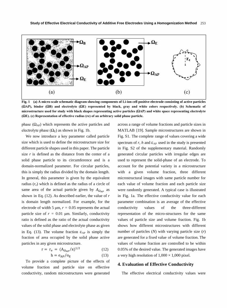
Fig. 1 (a) A micro-scale schematic diagram showing components of Li-ion cell positive electrode consisting of active particles
(ΩAP), binder (ΩB) and electrolyte (ΩE) represented by black, gray and white colors respectively. (b) Schematic of
microstructure used for study with black shapes representing active particles (ΩAP) and white space representing electrolyte
(ΩE). (c) Representation of effective radius (re) of an arbitrary solid phase particle.
phase (ΩAP) which represents the active particles and
electrolyte phase (ΩE) as shown in Fig. 1b.
We now introduce a key parameter called particle
size which is used to define the microstructure size for
different particle shapes used in this paper. The particle
size r is defined as the distance from the center of a
solid phase particle to its circumference and is a
domain-normalized parameter. For circular particles,
this is simply the radius divided by the domain length.
In general, this parameter is given by the equivalent
radius (re) which is defined as the radius of a circle of
same area of the actual particle given by as
shown in Eq. (12). As described earlier, the value of r
is domain length normalized. For example, for the
electrode of width 5 μm, r = 0.05 represents the actual
particle size of r = 0.01 μm. Similarly, conductivity
ratio is defined as the ratio of the actual conductivity
values of the solid phase and electrolyte phase as given
in Eq. (13). The volume fraction AP is simply the
fraction of area occupied by the solid phase active
particles in any given microstructure.
Ω (12)
σ σ (13)
To provide a complete picture of the effects of
volume fraction and particle size on effective
conductivity, random microstructures were generated
across a range of volume fractions and particle sizes in
MATLAB [19]. Sample microstructures are shown in
Fig. S1. The complete range of values covering a wide
spectrum of r, h and AP used in the study is presented
in Fig. S2 of the supplementary material. Randomly
generated circular particles with irregular edges are
used to represent the solid-phase of an electrode. To
account for the potential variety in a microstructure
with a given volume fraction, three different
microstructural images with same particle number for
each value of volume fraction and each particle size
were randomly generated. A typical case is illustrated
in Fig. 1a. The effective conductivity value for each
parameter combination is an average of the effective
conductivity values of the three-different
representation of the micro-structures for the same
values of particle size and volume fraction. Fig. 1b
shows how different microstructures with different
number of particles (N) with varying particle size (r)
are generated for a fixed value of volume fraction. The
values of volume fraction are controlled to be within
0.05% of the desired value. The generated images have
a very high resolution of 1,000 × 1,000 pixel.
4. Evaluation of Effective Conductivity
The effective electrical conductivity values were
Study of Effective Electrical Conductivity of Additive Free Electrodes Using a Homogenization Method
254
evaluated by the help of numerical simulation of the
randomly generated representative microstructures
shown in the previous section. Here we only present
concise results based on the extensive study carried out
over a range of values c.f. Fig. S2. To evaluate the
effective properties of the generated images, Eq. (12)
was solved using the MUMPS solver in COMSOL [15].
Mesh dependency tests were carried out and a very fine
triangular mesh with more than 0.32 million elements
was used for all analyses. Transport was assumed to be
dominant in horizontal (x-) direction. For each
combination of r, h and AP, three different instances of
the representative microstructure were simulated to
obtain three different values of effective electrical
conductivities. These estimates were then averaged to
obtain the averaged-effective conductivity value (σ*).
For simplicity, the averaged effective conductivity is
simply referred to as conductivity in the following
sections.
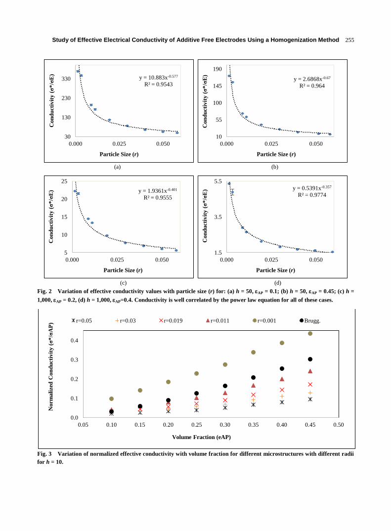
Fig. 2 shows the effect of particle size (r) on
conductivity for four different combinations of volume
fraction and conductivity ratios. As seen in this figure,
for a given volume fraction, when the particle size of
the solid phase decreases, leading to a greater number
of particles, conductivity increases. Conductivity is
directly related to the number of pathways available for
the transport of electrons. For a given volume fraction,
with smaller particle size, there are a large number of
particles in the domain (c.f. Fig. 1b) and as a result the
number of pathways increases exponentially. This in
turn increases the effective electrical conductivity. In
Fig. 1b, particle size of 0.001 (N = 19,000) corresponds
to a much larger number of particles available in the
domain compared to the microstructure geometry with
particle size of 0.04 (N = 50). Table 1 summarizes the
results from one combination of h and AP to illustrate
this. For same values of h and AP, decrease in particle
size from r = 0.05 to r = 0.0013 leads to more than
seven-fold increase in the conductivity. On the other
hand, Bruggeman’s relationship, shown in Case III for
these cases leads to a value of 0.2530 for both values of
r which highlights its limitation based on its inability to
incorporate the microstructure geometric information.
The error bars, shown as black vertical lines in Fig. 1
represent the variation in the values of σ* as a result of
averaging three different values from the three
respective random microstructure topologies for a
particular case.
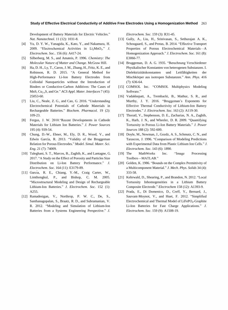
Fig. 3 illustrates the variation in the normalized
values of σ* with the change in volume fraction across
a range of particle sizes for two different values of h.
As expected effective conductivity is enhanced with
increasing volume fraction of the solid phase. A similar
trend is observed for all other values of h. The variation
of σ*, across a broad range of values of h, as a function
of volume fraction for r = 0.011 is shown in Fig. S3 of
the supplementary material. This trend is observed for
all other values of r considered in the study.
4.1 Comparison with Effective Bounds and
Bruggeman’s Formula
Effective property bounds of the randomly generated
microstructures provide the upper and lower limits of
the expected values of a given property. In this section,
we compare the results obtained for the calculation of
effective electrical conductivity for a range of
microstructures based on the proposed mathematical
homogenization method, Weiner bounds and
Bruggeman’s formula. The Weiner bounds provide the
limits of the values of effective properties by utilizing
the information on volume fraction and individual
conductivities [20]. These Weiner bounds for a
two-phase microstructure in terms of the conductivity
ratios are given as [13]:
σ σ (14)
σ σ (15)
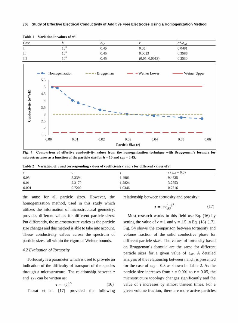
The comparison between the values for effective
conductivity obtained from homogenization method,
Weiner bounds and Bruggeman’s formula is shown in
Fig. 4. Since Weiner bounds and Bruggeman’s formula
only use the information of volume fraction and
individual conductivities, the values based on them are
Study of Effective Electrical Conductivity of Additive Free Electrodes Using a Homogenization Method
255
(a) (b)
(c) (d)
Fig. 2 Variation of effective conductivity values with particle size (r) for: (a) h = 50, AP = 0.1; (b) h = 50, AP = 0.45; (c) h =
1,000, AP = 0.2, (d) h = 1,000, AP=0.4. Conductivity is well correlated by the power law equation for all of these cases.
Fig. 3 Variation of normalized effective conductivity with volume fraction for different microstructures with different radii
for h = 10.
y = 10.883x-0.577
R² = 0.9543
30
130
230
330
0.000 0.025 0.050
Con
du
ctiv
ity
(σ
*/σ
E)
Particle Size (r)
y = 2.6868x-0.67
R² = 0.964
10
55
100
145
190
0.000 0.025 0.050
Con
du
ctiv
ity
(σ
*/σ
E)
Particle Size (r)
y = 1.9361x-0.401
R² = 0.9555
5
10
15
20
25
0.000 0.025 0.050
Con
du
ctiv
ity
(σ
*/σ
E)
Particle Size (r)
y = 0.5391x-0.357
R² = 0.9774
1.5
3.5
5.5
0.000 0.025 0.050
Con
du
ctiv
ity
(σ
*/σ
E)
Particle Size (r)
0.0
0.1
0.2
0.3
0.4
0.05 0.10 0.15 0.20 0.25 0.30 0.35 0.40 0.45 0.50
Norm
ali
zed
Con
du
ctiv
ity
(σ
*/σ
AP
)
Volume Fraction (eAP)
r=0.05 r=0.03 r=0.019 r=0.011 r=0.001 Brugg.
Study of Effective Electrical Conductivity of Additive Free Electrodes Using a Homogenization Method
256
Table 1 Variation in values of σ*.
Case h AP r σ*/σAP
I 106 0.45 0.05 0.0481
II 106 0.45 0.0013 0.3586
III 106 0.45 (0.05, 0.0013) 0.2530
Fig. 4 Comparison of effective conductivity values from the homogenization technique with Bruggeman’s formula for
microstructures as a function of the particle size for h = 10 and εAP = 0.45.
Table 2 Variation of τ and corresponding values of coefficients c and γ for different values of r.
r c γ τ ( AP = 0.3)
0.05 5.2394 1.4901 9.4525
0.01 2.3170 1.2824 3.2553
0.001 0.7209 1.0346 0.7516
the same for all particle sizes. However, the
homogenization method, used in this study which
utilizes the information of microstructural geometry,
provides different values for different particle sizes.
Put differently, the microstructure varies as the particle
size changes and this method is able to take into account.
These conductivity values across the spectrum of
particle sizes fall within the rigorous Weiner bounds.
4.2 Evaluation of Tortuosity
Tortuosity is a parameter which is used to provide an
indication of the difficulty of transport of the species
through a microstructure. The relationship between τ
and AP can be written as:
τ (16)
Thorat et al. [17] provided the following
relationship between tortuosity and porosity :
τ γ
(17)
Most research works in this field use Eq. (16) by
setting the value of c = 1 and γ = 1.5 in Eq. (18) [17].
Fig. S4 shows the comparison between tortuosity and
volume fraction of the solid conductive phase for
different particle sizes. The values of tortuosity based
on Bruggeman’s formula are the same for different
particle sizes for a given value of AP. A detailed
analysis of the relationship between τ and r is presented
for the case of AP = 0.3 as shown in Table 2. As the
particle size increases from r = 0.001 to r = 0.05, the
microstructure topology changes significantly and the
value of τ increases by almost thirteen times. For a
given volume fraction, there are more active particles
1.5
2
2.5
3
3.5
4
4.5
5
5.5
0.00 0.01 0.02 0.03 0.04 0.05 0.06
Con
du
ctiv
ity
(σ
*/σ
E)
Particle Size (r)
Homogenization Bruggeman Weiner Lower Weiner Upper

Study of Effective Electrical Conductivity of Additive Free Electrodes Using a Homogenization Method
257
available for electrical conduction when the size of
particles is small. However, when the size of the
particles increases, the number of active particles
distributed throughout the electrode becomes smaller.
This leads to a significantly fewer pathway for the
transport of electrons leading to a higher value of τ, i.e.,
a more tortuous path for the electrons to move. Now,
using the structure of Eq. (17), we can obtain the values
of the constants c and Bruggeman’s exponent γ for
each value of r as summarized in Table 2. These
expressions are very different from the one given in Eq.
(17). Kehrwald et al. [21] also reported similar
differences between their derived expressions and the
one described by Bruggeman’s relation. Similarly,
there is an increase in the possible conductive
pathways for the electrons to travel with the increase of
volume fraction. Hence, with the increase in the values
of AP, the values of τ decreases as shown in Fig. S4 of
the supplementary material.
4.3 Algebraic Formulation to Evaluate Effective
Conductivity
It is evident from the results of the previous sections,
the effective conductivity varies with the variation of
conductivity ratio, particle size and volume fraction of
active particles. The relationships between effective
conductivity and these three parameters are found to
follow certain trends across a wide spectrum of values
of h, r and AP. Based on these trends, we propose an
explicit formulation for the effective electrical
conductivity as a function of conductivity ratio h,
particle size r and volume fraction of solid phase AP:
σ (18)
Algebraic manipulations of the relationships
between σ* and h, r and AP lead to:
σ σ
(19)
where Ai and Bi are coefficients that are a function of h.
The coefficients Ai and Bi in Eq. (19) are found to
change with the variation in the values of conductivity
ratio. Fig. S5 of the supplementary material shows that
the variation of the coefficients of the formulation (A1,
A2, B1 and B2) across a range of values of h for h > 100
in log scale is in a perfect agreement with the trend line.
Based on this, these coefficients in general form can be
written as:
(20)
(21)
(22)
(23)
Similarly, an analysis was carried out for the values
of h ≤ 100, and coefficients in Eqs. (20)-(23) were
obtained. The values of the coefficients for the two
ranges of h are summarized in Table 3. In the next
section, a rigorous analysis of the proposed formulation
is carried out.
4.4 Analysis of the Proposed Formulation
In this section, we analyze the formulation proposed
in Eq. (19) that describes the effective electrical
conductivity as a function of particle size, volume
fraction and conductivity ratio. For the analysis, 200
different combinations of r, h and AP were considered.
Fig. 5 shows a comparison of the effective conductivity
values from Eq. (19) and the mathematical
homogenization method. An average relative error
value of approximately 8% was obtained. Major
sources of errors are the errors of estimate accumulated
because of the use of multiple trend lines for prediction
and the cut-off value for volume fraction (~0.05%)
used to save computational time.
To show that Eq. (19) proposed in this study is valid
of solid-phase particles of various shapes, three other
theoretical shapes of the active particles were considered.
Fig. 6a shows the representative microstructures with
these three shapes, namely square, triangle and circle.
The particle size for these shapes is defined according
to the definition provided in the representative
microstructure generation section. Effective conductivity
values were obtained for a range of values of h, r and
AP from mathematical homogenization technique
as well as the formulation proposed in Eq. (19).

Study of Effective Electrical Conductivity of Additive Free Electrodes Using a Homogenization Method
258
Table 3 Value of coefficients of the algebraic formula for calculation of effective conductivities.
h A11 A12 B11 B12 A21 A22 B21 B22
h ≤ 100 0.7136 0.4076 0.1189 0.3219 0.1676 0.4173 0.0379 0.17198
h > 100 0.0503 0.9885 0.4957 0.0014 1.7349 0.0079 0.0013 0.07232
Fig. 5 Comparison of the explicit formulation predicted values of conductivity normalized by conductivity ratio with the
actual values from simulation based on homogenization method across a range of values of h, r and εAP.
(a)
(b)
Fig. 6 (a) Microstructures of square, triangular and circular shapes from left to right with magnified views of shapes for
different values of r and ε. (b) Comparison between predicted values of normalized conductivity using proposed formulation
with actual values based on homogenization method for different shapes of solid-phase particles.
0
0.1
0.2
0.3
0.4
0.5
0 0.05 0.1 0.15 0.2 0.25 0.3 0.35 0.4 0.45 0.5
Pre
dic
ted
σ*
/σA
P
Actual σ*/σAP
Comparison 1:1
0
0.05
0.1
0.15
0.2
0.25
0 0.05 0.1 0.15 0.2 0.25
Pre
dic
ted
σ*
/σA
P
Actual σ*/σAP
Squares Triangles Circles 1:1
Study of Effective Electrical Conductivity of Additive Free Electrodes Using a Homogenization Method
259
A comparison of the results from Eq. (19) (predicted
values) and the homogenization technique (actual
values) is presented in Fig. 6b. Once again, we observe
a strong correlation between the actual and predicted
values. The average relative errors for the square,
triangular and circular shapes are approximately 11%,
8% and 14% respectively.
The proposed formula can be used to evaluate the
effective electrical conductivity of the positive
electrode of a Li-ion battery consisting of electrolyte
and the active materials as discussed. However, the
Li-ion batteries in use now also include three phases.
Fig. S6 shows typical positive electrode microstructure
images as it undergoes changes during a typical charge
and discharge cycle. Although this formulation cannot
be directly used for the evaluation of effective
electrical conductivity because of the presence of the
binder phase, it can prove useful for additive-free
cathodes as discussed earlier. Hence, it provides an
easy way to evaluate the effective electrical
conductivity of a cathode consisting of two distinct
phases viz. electrolyte and active particles.
5. Application Performance of a Li-ion Cell
Model
In this section, we illustrate the application of the
proposed formulation by providing the results and
analysis of a Li-ion cell model which is based on the
study on P2D model developed by Doyle et al. [18].
This model is based on the principles of electrochemistry,
transport phenomena and thermodynamics and has
been extensively used to study battery models. Taleghani
et al. [10] used this model to study the effects of porosity
and particle size distribution on the performance of
Li-ion battery. Similarly, Prada et al. [22] used this model
to provide a simplified model for LiFePO4-graphite
Li-on batteries. Here, we study the influence of
microstructure on cell discharge characteristics using
this P2D model. Mono-modal particle size distribution
is considered for the study. This section aims to
highlight the importance of accurate prediction of
effective properties by considering the microstructure
geometry using the effective property values evaluated
using the proposed formulation based on the
mathematical homogenization method. We also
highlight the limitation of Bruggeman’s formula on
battery performance prediction.
The schematic diagram model of Li-ion battery
considered for study is shown in Fig. 7. This model is
based on a study carried out by Doyle et al. [18]. Here,
we use two distinct phases as described earlier and
consider the active particles and electrolyte in both
electrodes. LiPF6 salt dissolved in organic solvent 1:2
v/v mixture of EC: DMC with the polymer matrix,
p(VdF-HFP) is the electrolyte used in this study. The
negative electrode is composed of carbon-based
material whereas the positive electrode consists of
LixMn2O4.
Values of different parameters used in this study are
summarized in Table 4. Most of the parameters
including the properties of electrodes and electrolyte
used here are based on the study by Doyle et al. [18].
For all other key parameters used in this
electrochemical model, the reader is referred to
COMSOL’s documentation [15].
In the study, electrical conductivity of electrolyte is
assumed to be 10-8
. This value leads to a conductivity
ratio h of nearly 108 and 10
10 for positive and negative
electrodes respectively. This value is generally
assumed to be zero in literature. But the
homogenization method used in this study does not
allow us to consider a value of zero [13]. Here, we only
modify effective electrical conductivity using the
proposed homogenization-based formulation. The
results based on the effective conductivity calculated
using homogenization method are then compared to the
results obtained based on the correction given by
Bruggeman’s formula. Effective values of ionic
conductivity and diffusivity are based on Bruggeman’s
formula by default and are unchanged. The MUMPS
direct solver is used for all simulations in COMSOL for
this study [15].

Study of Effective Electrical Conductivity of Additive Free Electrodes Using a Homogenization Method
260
Fig. 7 Schematic diagram of Li-ion cell consisting of positive electrode, separator and negative electrode. The positive and
negative porous electrodes both are shown to consist of two phases with the white phase representing electrolyte.
The dark circular inclusions denote the active materials which are carbon and lithium manganese dioxide particles for positive and
negative electrodes respectively. The current collectors for the negative and positive electrodes are represented by – and + respectively.
Table 4 Key parameters for the electrodes.
Parameter Positive electrode Negative electrode
Active material LixMn2O4 LixC6
L* 174 μm 100 μm
σAP 3.8 S/m 100 S/m
rp 8.5 μm 12.5 μm
AP 0.3 0.45
E 0.7 0.55
h 3.8 × 10⁸ 1010
*The width of separator is 52 μm.
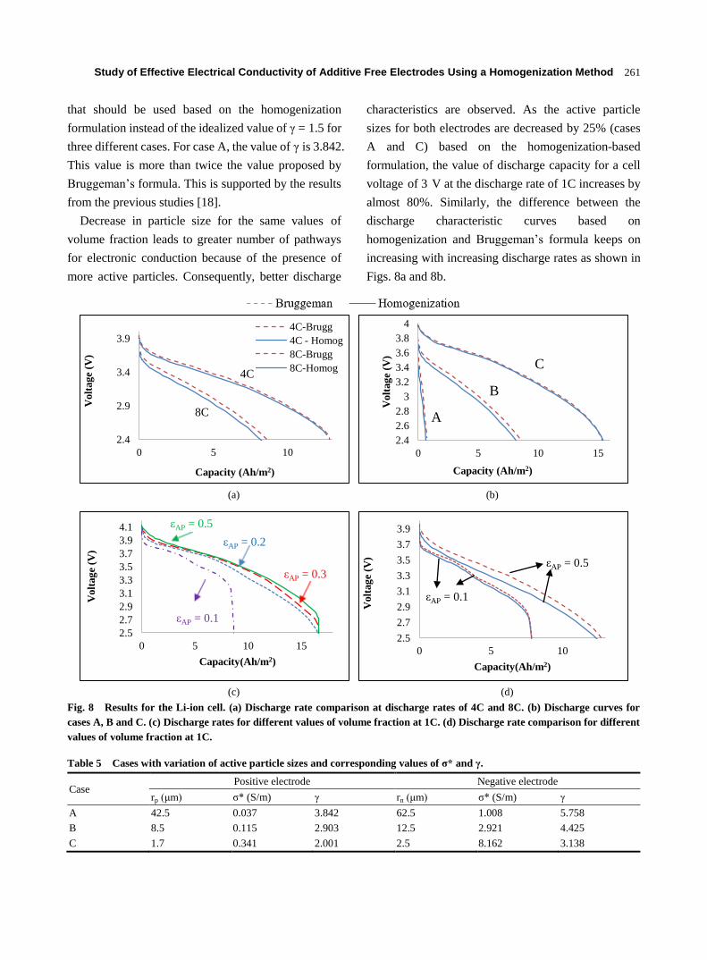
In Fig. 8a, we show the discharge curves at the
discharge rates of 4C and 8C using the effective
electrical conductivity values calculated using the
Bruggeman’s formula and the proposed
homogenization-based formulation. In this case, the
theoretical 1C-rate current density is 17.5 A/m2 [18].
The discharge capacity decreases at an increasing rate
for a given cell voltage when the discharge rate
increases from 4C to 8C. The cell discharge capacity
decreases by 65% at a discharge rate of 8C as
compared to that at 1C based on Bruggeman’s estimate
at 3V. On the other hand, this change in discharge
capacity is 69% when we use the
homogenization-based formulation.
At 8C, the 3V discharge capacity of the cell is almost
14% lower based on homogenization approach as
compared to Bruggeman’s formula. And this
difference at different cell voltage values increases
with increasing discharge rate as shown in Fig. 5. It is
important to note that this deviation could be even
larger if we were to use the homogenization approach
for the evaluation of effective diffusivity and
electrolyte conductivities. This further highlights the
need for the use of microstructure geometry
information while evaluating the effective properties.
In Fig. 8c, we show the discharge characteristics
with the change in the active particle sizes at 1C. Table
5 includes the values of the Bruggeman’s exponent (γ)
LP LS LN
Negative Electrode Separator Positive Electrode
Study of Effective Electrical Conductivity of Additive Free Electrodes Using a Homogenization Method
261
that should be used based on the homogenization
formulation instead of the idealized value of γ = 1.5 for
three different cases. For case A, the value of γ is 3.842.
This value is more than twice the value proposed by
Bruggeman’s formula. This is supported by the results
from the previous studies [18].
Decrease in particle size for the same values of
volume fraction leads to greater number of pathways
for electronic conduction because of the presence of
more active particles. Consequently, better discharge
characteristics are observed. As the active particle
sizes for both electrodes are decreased by 25% (cases
A and C) based on the homogenization-based
formulation, the value of discharge capacity for a cell
voltage of 3 V at the discharge rate of 1C increases by
almost 80%. Similarly, the difference between the
discharge characteristic curves based on
homogenization and Bruggeman’s formula keeps on
increasing with increasing discharge rates as shown in
Figs. 8a and 8b.
(a) (b)
(c) (d)
Fig. 8 Results for the Li-ion cell. (a) Discharge rate comparison at discharge rates of 4C and 8C. (b) Discharge curves for
cases A, B and C. (c) Discharge rates for different values of volume fraction at 1C. (d) Discharge rate comparison for different
values of volume fraction at 1C.
Table 5 Cases with variation of active particle sizes and corresponding values of σ* and γ.
Case Positive electrode Negative electrode
rp (μm) σ* (S/m) γ rn (μm) σ* (S/m) γ
A 42.5 0.037 3.842 62.5 1.008 5.758
B 8.5 0.115 2.903 12.5 2.921 4.425
C 1.7 0.341 2.001 2.5 8.162 3.138
2.4
2.9
3.4
3.9
0 5 10
Volt
ag
e (V
)
Capacity (Ah/m2)
4C-Brugg
4C - Homog
8C-Brugg
8C-Homog 4C
8C
2.4
2.6
2.8
3
3.2
3.4
3.6
3.8
4
0 5 10 15
Volt
ag
e (V
)
Capacity (Ah/m2)
C
B
A
2.5
2.7
2.9
3.1
3.3
3.5
3.7
3.9
4.1
0 5 10 15
Volt
ag
e (V
)
Capacity(Ah/m2)
AP = 0.5
AP = 0.3
AP = 0.2
AP = 0.1
2.5
2.7
2.9
3.1
3.3
3.5
3.7
3.9
0 5 10
Volt
ag
e (V
)
Capacity(Ah/m2)
AP = 0.5
AP = 0.1

Study of Effective Electrical Conductivity of Additive Free Electrodes Using a Homogenization Method
262
As a result of the increase in volume fraction means,
greater amount of active materials become available
for conduction. This leads to better discharge
characteristics. In Fig. 8c, we show the discharge
curves by varying only the volume fraction and
corresponding effective electrode conductivity for the
positive electrode only using the proposed formulation
at a discharge rate of 1C. With the increase in volume
fraction of the active particles in the positive electrode,
a considerable improvement in the discharge
characteristics can be observed. At 3 V cell voltage, the
capacity increases by 76% as this volume fraction
increases from 0.1 to 0.5. In Fig. 8d, we show the
discharge characteristics for different values of volume
fractions using both the described methods. It can be
observed that for both values of volume fraction,
values based on Bruggeman’s formula overpredict the
voltage at a given discharge capacity.
6. Summary and Conclusions
In this study, the focus has been on two-phase
electrodes without any additives to enhance
conductivity. We show that by carefully engineering
the microstructures, we can enhance the effective
properties. To this end, we have carried out an
extensive analysis of the effective electrical
conductivity of randomly generated microstructures
idealized for Li-ion battery electrodes using
mathematical homogenization based approach. The
Bruggeman’s formula cannot factor in the change in
microstructure geometry. Therefore, it is only able to
predict a constant value of effective conductivity for all
particle sizes. On the other hand, homogenization
based technique considers the microstructure geometry
and gives different values based on microstructure
geometry.
From the results of mathematical homogenization, to
provide a simple method for the evaluation of effective
electrical conductivity of an electrode of a Li-ion
battery based on the conducting solid phase and
non-conducting electrolyte phase, we have proposed an
explicit formula relating effective conductivity with
conductivity ratio of phases, particle size and volume
fraction of active phase. We have also carried out an
analysis of the proposed formulation showing a very
good agreement with the actual values based on
homogenization method for a mono-modal particle size
distribution.
To highlight the applicability of the proposed
formulation, the discharge characteristics were studied
for a Li-ion battery based on the P2D model. We
present the differences in the discharge curves when
the microstructural effect is considered with the
homogenization method and when it is not using the
Bruggeman’s formula. It was observed that the
variation between results of discharge characteristics
based on these two approaches is more significant at
higher discharge rates and for higher volume fraction
of active particles.
A possible extension to this work could be to include
multi-modal particle size distribution to provide a more
accurate representation of the effective values.
Similarly, in order to overcome the limitation with the
confinement of transport of properties in a single plane,
results for the evaluation of the effective electrical
conductivity based on the depth of the electrodes can
be studied in the future. Finally, inclusion of other
effective properties including diffusivity and ionic
conductivity would be able to provide a more accurate
description of the discharge characteristics of the
battery model.
Acknowledgments
Both authors are grateful to NSERC for funding this
work via the Discovery grant program.
References
[1] U.S. Energy Information Administration,2016.
“International Energy Outlook 2016”.
[2] World Energy Council. 2016. “World Energy Scenarios
2016”.
[3] Lu, J., Chen, Z., Ma, Z., Pan, F., Curtiss, L. A., and Amine,
K. 2016. “The Role of Nanotechnology in the
Study of Effective Electrical Conductivity of Additive Free Electrodes Using a Homogenization Method
263
Development of Battery Materials for Electric Vehicles.”
Nat. Nanotechnol. 11 (12): 1031-8.
[4] Yu, D. Y. W., Yanagida, K., Kato, Y., and Nakamura, H.
2009. “Electrochemical Activities in Li2MnO3.” J.
Electrochem. Soc.. 156 (6): A417-24.
[5] Silberberg, M. S., and Amateis, P. 1996. Chemistry: The
Molecular Nature of Matter and Change. McGraw Hill.
[6] Ha, D. H., Ly, T., Caron, J. M., Zhang, H., Fritz, K. E., and
Robinson, R. D. 2015. “A General Method for
High-Performance Li-Ion Battery Electrodes from
Colloidal Nanoparticles without the Introduction of
Binders or Conductive-Carbon Additives: The Cases of
MnS, Cu2-xS, and Ge.” ACS Appl. Mater. Interfaces 7 (45):
25053-60.
[7] Liu, C., Neale, Z. G., and Cao, G. 2016. “Understanding
Electrochemical Potentials of Cathode Materials in
Rechargeable Batteries.” Biochem. Pharmacol. 19 (2):
109-23.
[8] Fergus, J. W. 2010.“Recent Developments in Cathode
Materials for Lithium Ion Batteries.” J. Power Sources
195 (4): 939-54.
[9] Chung, D.-W., Ebner, M., Ely, D. R., Wood, V., and
Edwin García, R. 2013. “Validity of the Bruggeman
Relation for Porous Electrodes.” Model. Simul. Mater. Sci.
Eng. 21 (7): 74009.
[10] Taleghani, S. T., Marcos, B., Zaghib, K., and Lantagne, G.
2017. “A Study on the Effect of Porosity and Particles Size
Distribution on Li-Ion Battery Performance.” J.
Electrochem. Soc. 164 (11): E3179-89.
[11] arc a, R. E., Chiang, Y.-M., Craig Carter, W.,
Limthongkul, P., and Bishop, C. M. 2005.
“Microstructural Modeling and Design of Rechargeable
Lithium-Ion Batteries.” J. Electrochem. Soc. 152 (1):
A255.
[12] Ramadesigan, V., Northrop, P. W. C., De, S.,
Santhanagopalan, S., Braatz, R. D., and Subramanian, V.
R. 2012. “Modeling and Simulation of Lithium-Ion
Batteries from a Systems Engineering Perspective.” J.
Electrochem. Soc. 159 (3): R31-45.
[13] Gully, A., Liu, H., Srinivasan, S., Sethurajan A. K.,
Schougaard, S., and Protas, B. 2014. “Effective Transport
Properties of Porous Electrochemical Materials—A
Homogenization Approach.” J. Electrochem. Soc. 161 (8):
E3066-77.
[14] Bruggeman, D. A. G. 1935. “Berechnung Verschiedener
Physikalischer Konstanten von heterogenen Substanzen. I.
Dielektrizitätskonstanten und Leitfähigkeiten der
Mischkörper aus isotropen Substanzen.” Ann. Phys. 416
(7): 636-64.
[15] COMSOL Inc. “COMSOL Multiphysics Modeling
Software.”
[16] Vadakkepatt, A., Trembacki, B., Mathur, S. R., and
Murthy, J. Y. 2016. “Bruggeman’s Exponents for
Effective Thermal Conductivity of Lithium-Ion Battery
Electrodes.” J. Electrochem. Soc. 163 (2): A119-30.
[17] ThoratI, V., Stephenson, D. E., Zacharias, N. A., Zaghib,
K., Harb, J. N., and Wheeler, D. R. 2009. “Quantifying
Tortuosity in Porous Li-Ion Battery Materials.” J. Power
Sources 188 (2): 592-600.
[18] Doyle, M., Newman, J., Gozdz, A. S., Schmutz, C. N., and
Tarascon, J. 1996. “Comparison of Modeling Predictions
with Experimental Data from Plastic Lithium Ion Cells.” J.
Electrochem. Soc. 143 (6): 1890.
[19] The MathWorks Inc. “Image Processing
Toolbox—MATLAB.”
[20] Golden, K. 1986. “Bounds on the Complex Permittivity of
a Multicomponent Material.” J. Mech. Phys. Solids 34 (4):
333-58.
[21] Kehrwald, D., Shearing, P., and Brandon, N. 2012. “Local
Tortuosity Inhomogeneities in a Lithium Battery
Composite Electrode.” Electrochem 158 (12): A1393-9.
[22] Prada, E., Di Domenico, D., Creff, Y., Bernard, J.,
Sauvant-Moynot, V., and Huet, F. 2012. “Simplified
Electrochemical and Thermal Model of LiFePO4-Graphite
Li-Ion Batteries for Fast Charge Applications.” J.
Electrochem. Soc. 159 (9): A1508-19.

Study of Effective Electrical Conductivity of Additive Free Electrodes Using a Homogenization Method
264
Supplementary Material
(a)
(b)
Fig. S1 Microstructures generated for study. (a) Three iterations for the same radius of 0.06 and volume fraction of 0.25 with
magnified view of one solid phase particle with irregular edges. (b) Different microstructures for same volume fraction but
different radii of approximately 0.04 (N = 50), 0.011 (N = 553) and 0.001 (N = 19,894) respectively from left to right.
Fig. S2 Range of values used for study. The values of conductivity ratio (h) are represented in Log10 scale. A total of 720
distinct combinations of h, r and ε used for the study and 3 randomly generated microstructures were used for each
combination to evaluate the averaged effective conductivity.
Study of Effective Electrical Conductivity of Additive Free Electrodes Using a Homogenization Method
265
Fig. S3 Effective conductivity as a function of volume fraction for different values of conductivity ratios (r = 0.011).
Fig. S4 Comparison of tortuosity vs. volume fraction for different radii based on the mathematical homogenization method
with Bruggeman’s formula for different microstructures with different radii for h = 107.
1.0E+00
1.0E+01
1.0E+02
1.0E+03
1.0E+04
1.0E+05
0.10 0.15 0.20 0.25 0.30 0.35 0.40 0.45
Log
of
Con
du
ctiv
ity
(L
og
10
σ*
/σA
P)
Volume Fraction (eAP)
h=10 h=100 h=1000 h=10000 h=100000

Study of Effective Electrical Conductivity of Additive Free Electrodes Using a Homogenization Method
266
Fig. S5 Variation of the coefficients of formulation A1, A2, B1 and B2 across a range of values of h for h > 100. For clarity of
representation, both axes are presented in logarithmic scale and the y-axis values are scaled by h.
Fig. S6 Processed representative images of a Li-ion positive electrode taken at various stages of the cycling process.
y = 1.075x1.0013
R² = 1
1.E+03
1.E+04
1.E+05
1.E+06
1.E+07
1.00E+03 1.00E+05 1.00E+07
heB
2
h
y = 1.7349x1.0079
R² = 1
1.E+03
1.E+04
1.E+05
1.E+06
1.E+07
1.00E+03 1.00E+05 1.00E+07
hA
2
h
y = 0.4957x1.0014
R² = 1
5.E+02
5.E+03
5.E+04
5.E+05
5.E+06
1.00E+03 1.00E+05 1.00E+07
-hB
1
h
y = 0.0503x1.9885
R² = 1
4.E+04
4.E+05
4.E+06
4.E+07
4.E+08
4.E+09
4.E+10
4.E+11
4.E+12
1.00E+03 1.00E+05 1.00E+07
hA
1
h