James Madison UniversityJMU Scholarly Commons

Senior Honors Projects, 2010-current Honors College

Spring 2017

Studies into the structure and function of variousdomains of obscurin and titinRachel A. PolickeJames Madison University

Follow this and additional works at: https://commons.lib.jmu.edu/honors201019Part of the Biochemistry Commons

This Thesis is brought to you for free and open access by the Honors College at JMU Scholarly Commons. It has been accepted for inclusion in SeniorHonors Projects, 2010-current by an authorized administrator of JMU Scholarly Commons. For more information, please contactdc_admin@jmu.edu.

Recommended CitationPolicke, Rachel A., "Studies into the structure and function of various domains of obscurin and titin" (2017). Senior Honors Projects,2010-current. 376.https://commons.lib.jmu.edu/honors201019/376

1

Studies into the Structure and Function of Various Domains of Obscurin and Titin

———————————————

A Project Presented to

The Faculty of the Undergraduate

College of Chemistry and Biochemistry

James Madison University

——————————————

In Partial Fulfillment of the Requirements

For the Degree of Bachelor of Sciences

—————————————

By Rachel A. Policke

April 2017

Accepted by the faculty of the Department of Chemistry and Biochemistry, James Madison

University, in partial fulfillment of the requirements for the Degree of Bachelor of Sciences.

FACULTY COMMITTEE: HONORS PROGRAM APPROVAL:

Project Advisor: Nathan T. Wright, Ph.D Date Bradley Newcomer, Ph.D Date

Assistant Professor, Chemistry and Biochemistry Dean of the Honors College, Honors Program

Reader: Christopher E. Berndsen, Ph.D Date

Assistant Professor, Chemistry and Biochemistry

Reader: Isaiah Sumner, Ph.D Date

Assistant Professor, Chemistry and Biochemistry

2

Table of Contents

List of Tables and Figures 3

Acknowledgements 5

Preface/Introduction 6

A Variant in the Obscurin Gene Associated with a Frameshift Mutation in the

Filamin C Gene in a Family with Distal Muscular Dystrophy 15

Studies on the Molecular Motion, Structure, and Elasticity of Titin 33

Insight into the Auto-inhibitory Mechanism of the Second Kinase Domain of Obscurin 40

Appendices 47

Appendix A: Methods for Additional Projects 47

Appendix B: Tutorial on How to Solve a Crystal Structure using HKL2000,

Phenix, and Coot 49

Appendix C: Tutorial on How to Make Publication Quality Images in PyMOL 61

References 62

3

List of Tables and Figures

Schematic representation of muscle structure 5

Steps of muscle contraction 5

Schematic representation of a sarcomere 6

Cartoon of Ig domain and Fn-III-like domain 7

Schematic of titin and its binding partners 7

Schematic of obscurin and its binding partners 8

Comparison of normal muscle vs muscle with MD 8

Comparison of normal heart vs heart with HCM 9

Table of genes associated with MD 14

Table of refinement statistics of obscurin Ig59 20

Table of clinical measurements of proband 23

Clinical data, morphological studies, and ultrastructural studies of proband 24

Genetic analysis of OBSCN c.13330 C>T and FLNC c.5161delG mutations 25

Structure and analysis of Ig59 26

NMR data of Ig59 27

Table of NMR-derived statistics of 20 NMR structures of Ig59 28

Linker regions of I6 32

I6 crystal structure statistics after refinement 34

Depictions of I6 B-factors 35

Crystal packing of I6 36

Alignment of 2RIK with 3B43 36

Snapshots of I6 equilibration 37

Force vs distance graph and snapshots of I6 compression 38

Schematic of titin and obscurin kinase regions 39

Gel showing KII autophosphoryation and phosphorylation of cadherin 40

Surface views of inhibited conformation of titin 40

Sequence of KII with active, NL, and CL residues labeled 42

Structure of titin and obscurin kinases 44

Overlay of average and last KII equilibration structures 44

4

Model and HADDOCK graph of NL tests 45

Model and HADDOCK graph of CL tests 45

5

Acknowledgements

I would like to thank Dr. Nathan Wright, Dr. Christopher Berndsen, and Dr. Isaiah Sumner for

serving on my senior project committee as well as for all of their help and guidance in writing

and editing my senior project. Additionally, I would like to extend thanks to Dr. Nathan Wright

for guidance in my four years of undergraduate research, Dr. Christopher Berndsen for help

with crystallography, and Dr. Isaiah Sumner for help with simulations, as well as the entire

James Madison University Department of Chemistry and Biochemistry for their support and

use of instrumentation. This work was supported by the Jeffress Memorial Trust J-1041 (to

NTW), Research Corporation 22450 (to NTW) and James Madison University startup funds (to

NTW, CEB, and IS).

6

Abstract

Muscles give our bodies the ability to move by stretching and contracting. While

contraction is accomplished by the well-known actin-myosin interaction, not much is known

about stretch. Two integral muscle proteins involved in stretch are titin and obscurin; both are

long rope-like protein molecules that seem to act as molecular springs. Mutations in these two

proteins can lead to diseases such as hypertrophic cardiomyopathy and muscular dystrophy, as

well as a variety of cancers. In an effort to understand muscle stretch and signaling on a more

fundamental level, here we present the high resolution structure of obscurin Ig59, a domain

involved in titin/obscurin binding. We also describe how unbound titin moves when stretched.

Last, we describe ongoing work in elucidating the high-resolution structures and

activation/inhibition mechanisms of obscurin domains Rho-GEF, Rho-GEF-PH, kinase I (KI),

and kinase II (KII).

7

Preface/Introduction

Muscles, Muscle Proteins, and Structure of the Sarcomere

Muscles give our bodies the ability to move by stretching and contracting. Without

them, we would not be able to walk, stand up, or perform any of the motions do throughout our

daily lives. Striated muscles, the ones connected to our skeleton, allow for virtually all

voluntary movement of our body. As the name implies, this kind of muscle is made up of a

series of different bands that are visible in the light microscope, termed the A-band and the I-

band. One A-band and half of the neighboring I-band form the sarcomere, the smallest

contracting segment of muscle. Hundreds of sarcomeres lie end-to-end, making up the syncytial

cell type called the myofibril. These cell types are the largest in the human body; the longest

can be more than a foot long. Many myofibrils are bundled together into a single fascicle,

which in turn is bundled into a muscle (Fig. 1).

When a muscle

contracts, myosin thick

filaments slide across F-actin

thin filaments in an ATP- and

calcium-requiring reaction,

resulting in a shortening of

the sarcomere. This process,

termed the sliding filament

model, involves a number of

simple steps to produce

contraction. When the brain

generates an electrical signal

in the form of an action

potential, it courses along

through the somatic nervous

system to the axon of a motor

neuron, which is connected to

a skeletal muscle cell.

Acetylcholine is released by

neurotransmitters within the

Figure 1. Schematic representation of the muscle, showing its breakdown into fascicles, fibers, and sarcomeres (adapted from John Wiley & Sons, Inc., 2013).

Figure 2. Steps of muscle contraction showing the process of calcium release and binding to troponin, conformation changes of troponin and tropomyosin, hydrolysis of ATP, power stroke, binding of ATP to myosin, and release of bound calcium from troponin (taken from https://mykindofscience.com/2015/01/20/my-awe-of-the-human-body-muscle-movement-2/).

8

synaptic cleft, which binds to membrane proteins in the outer layer of the muscle cell,

depolarizing it. This depolarization allows the action potential to travel into the cell and activate

Ryanodine receptor-dependent calcium channels within the sarcoplasmic reticulum. Calcium

ions flow into the muscle cell as a result and bind to troponin in the thin filament region of the

muscle cell. The calcium binding induces a conformation change in the troponin protein, which

in turn alters the tropomyosin-actin interaction. The new conformation of tropomyosin exposes

the myosin binding sites on actin (the thin filament). Once the myosin binding sites are

exposed, head structures on the myosin molecules hydrolyze bound ATP and reorient to bind to

actin. Finally, release of ADP and Pi from the myosin head generates a power stroke (Fig. 2,

steps 1 and 2) that brings adjacent Z lines closer to each other, shortening the length of the

sarcomere and contracting the cell (Fig. 2, step 3. The cell returns to a relaxed state when ATP

binds to myosin and the calcium ion bound to troponin is released (Fig. 2, step 4).

In order for these ultrastructural filaments to perform their jobs and contribute to overall

muscle contraction, the sarcomere must be exquisitely well ordered. If the thick filaments did

not interdigitate the thin filaments, there would be no contraction. Similarly, if the thick and

thin filaments did not overlap, there would be no power stroke. The almost paracrystalline-like

array of contractile apparatus is accomplished through the cytoskeleton; particularly, through

the involvement of the giant cytoskeletal proteins titin, nebulin, and obscurin.

Titin, the longest known polypeptide at 3-5 MDa, has its N- and C-termini anchored in

the Z-disc and M-line, respectively. Titin generates passive elasticity of muscles by acting as a

force sensor and regulates the length of the thick filament of the sarcomere (Trinick, 1992; Hsin

et al., 2011; Fig. 3, red). Throughout its considerable length, it binds to and anchors many

proteins to the surrounding cytoskeleton and acts as a molecular spring, regulating amount of

stretch in the sarcomere. Nebulin (600-800 kDa) stabilizes the thin filament and may also have

some function in regulating the length of the thin filament, directing actin/myosin interactions,

and myofibrillar force generation (Trinick, 1992; Chu et al., 2016; Kontrogianni-

Konstantopoulos et al., 2009). Last, obscurin connects the sarcomere to the surrounding

sarcoplasmic reticulum via its interaction with titin (Fig. 3) and aids in assembly of myofibrils

and the sarcoplasmic reticulum (Meyer and Wright, 2003; Lee et al., 2010; Bang et al., 2001;

Young et al., 2001; Armani et al., 2006; Kontrogianni-Konstantopoulos and Bloch, 2009).

Obscurin and titin are the focus of

my research.

Due to their large size and

complexity, titin and obscurin have

been difficult to study using

traditional molecular biology or

biochemistry techniques. However,

both are highly modular in overall

architecture. Titin has

approximately 300 independently

folded domains while obscurin has

at least 70, though the exact number

depends on the isoform; each

domain of titin consists of

approximately 100 amino acids

(Meyer and Wright, 2013). The

most common folds are the

immunoglobulin (Ig) and

Fibronectin typeIII-like (FnIII-like)

domains, which both fold into

variations of a β-sandwich fold.

Figure 3. Schematic representation of the sarcomere. Titin (red)

anchors the M-line and Z-disc and regulates the length of the sarcomere. Obscurin (blue) tethers titin to the sarcoplasmic reticulum. Nebulin (green) regulates the length of the thin filaments (actin, under the green). Myosin heads (grey) slide across the thin filaments as a muscle contracts (taken from Meyer and Wright, 2013).

9

(Meyer and Wright, 2003; Fig. 4). Rather than trying to discern structure/function relationships

of the entire obscurin or titin molecule, we (and others) have instead found it more useful to

focus on solving the high-resolution structure of individual domains. In other words, we choose

to describe the obscurin and titin structure/function relationship from a bottom-up approach,

from domains to whole molecules. To this end, I will begin with an overview of titin and

obscurin, their associated diseases and then move onto a more in-depth discussion of obscurin.

Titin

is found

mostly in

skeletal and

cardiac

muscle tissue

and spans the

sarcomere

from the Z-

disk to the

M-band

(Bang et al.,

2001;

Granzier and

Wang, 1993;

Linke, 1994; Kontrogianni-Konstantopoulos et al., 2009). In the body, titin regulates the length

of the sarcomere and helps restore the pre-contraction length, protecting the sarcomere from

injury caused by overstretching (Lee et al., 2010). Titin’s ability to both stretch and recoil is

fundamental in preventing muscle overstretching, and helps myocytes return to their original

length (Gautel, 2011; Improta et al. 1998). In this capacity, titin acts as a mechanosensor

(Kontrogianni-Konstantopoulos et al., 2009; Linke 2008; Meyer and Wright, 2003).

Figure 5. Schematic representation of the structure and binding partners of titin A-M (the portion of titin spanning from the A-line to the M-line). Note that the key provided lists the domain types as well as the meaning of the colors and shapes used in the schematic (adapted from Kontrogianni-Konstantopoulos, 2009).

A decidedly important player in muscle contraction, titin has a multitude of binding

partners, one of which is obscurin (Fig. 6). Obscurin (~720-900 kDa) is made up of mostly Ig

domains and binds to titin in the Z-disk region of the sarcomere (Young et al., 2001; Bang et

al., 2001) (Fig. 5&6). With titin bound at its N-terminus and small ankyrin bound at its C-

terminus, obscurin effectively connects titin to the sarcoplasmic reticulum (Bang et al., 2001;

Young et al., 2001; Armani et al., 2006; Kontrogianni-Konstantopoulos et al., 2009) (Fig. 6).

Figure 4. Cartoon representation and schematic of A.) an Ig domain and B.) a FnIII-

like domain. The cartoon representations are colored from N-terminus (blue) to C-

terminus (red) (adapted from Meyer and Wright).

10

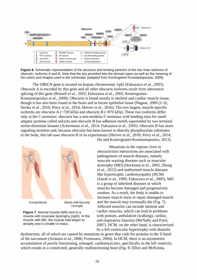
Figure 6. Schematic representation of the structure and binding partners of the two main isoforms of obscurin, isoforms A and B. Note that the key provided lists the domain types as well as the meaning of the colors and shapes used in the schematic (adapted from Kontrogianni-Konstantopoulos, 2009).

The OBSCN gene is located on human chromosome 1q42 (Fukuzawa et al., 2005).

Obscurin A is encoded by this gene and all other obscurin isoforms result from alternative

splicing of this gene (Russell et al., 2002; Fukuzawa et al., 2005; Kontrogianni-

Konstantopoulos et al., 2009). Obscurin is found mostly in skeletal and cardiac muscle tissue,

though it has also been found in the brain and in breast epithelial tissue (Nagase, 2000 (1-3);

Stroka et al., 2016; Perry et al., 2014; Shriver et al., 2016). The two largest, muscle-specific

isoforms are obscurin A (~720 kDa) and obscurin B (~870 kDa). These two isoforms differ

only at the C-terminus: obscurin has a non-modular C-terminus with binding sites for small

adaptor proteins called ankyrin and obscurin B has adhesion motifs superseded by two terminal

serine-threonine kinases (Ackermann et al., 2014; Fukuzawa et al., 2005). Obscurin B has more

signaling moieties and, because obscurin has been known to directly phosphorylate substrates

in the body, this lab uses obscurin B in its experiments (Shriver et al., 2016; Perry et al., 2014;

Hu and Kontrogianni-Konstantopoulos, 2013).

Mutations in the regions close to

obscurin/titin interactions are associated with

pathogenesis of muscle diseases, namely

muscule wasting diseases such as muscular

dystrophy (MD) (Hackman et al., 2002; Zheng

et al., 2015) and malformed muscle diseases

like hypertrophic cardiomyopathy (HCM)

(Satoh et al., 1999; Fukuzawa et al., 2005). MD

is a group of inherited diseases in which

muscles become damaged and progressively

weaken. As a result, the body is unable to

increase muscle mass or repair damaged muscle

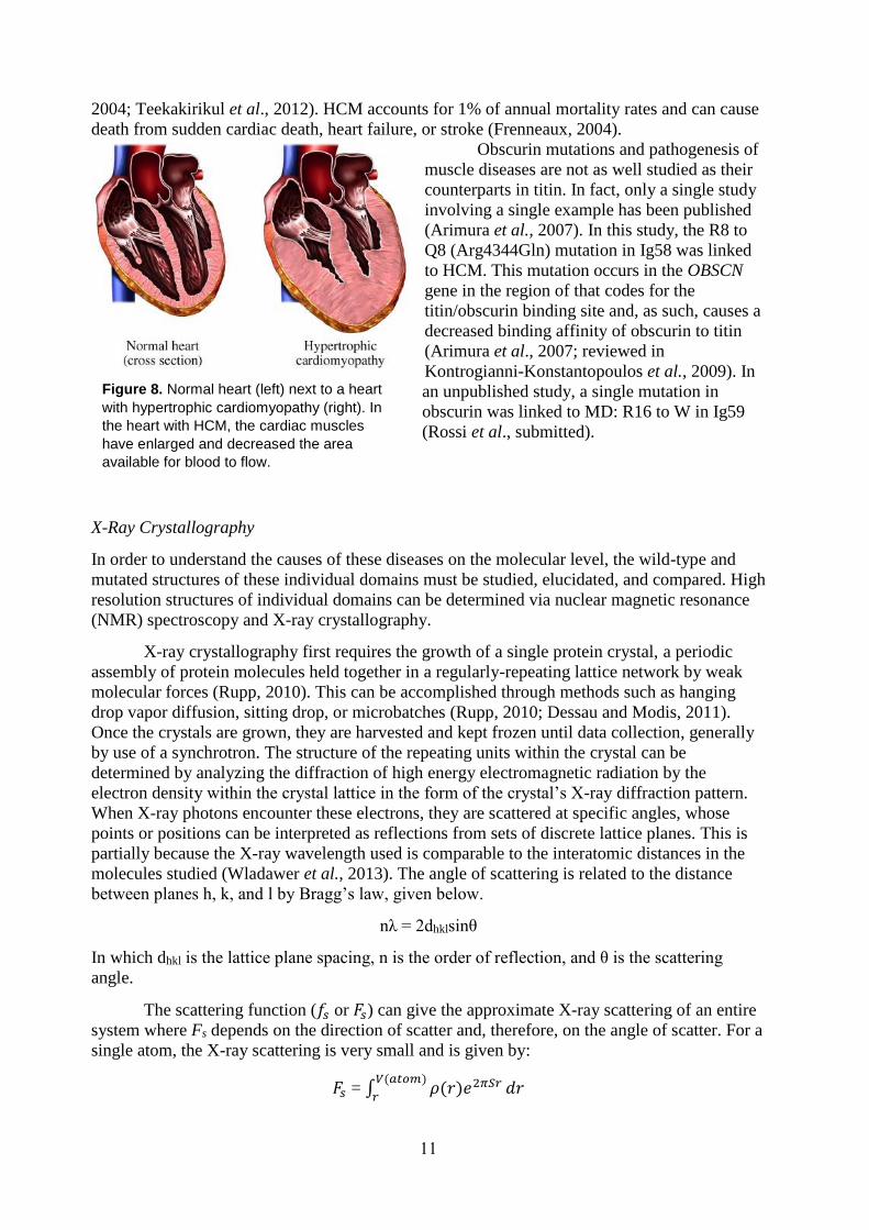
and the muscle may eventually die (Fig. 7).

Affected muscles can include skeletal and

cardiac muscles, which can lead to problems

with posture, ambulation (walking), cardiac,

and respiratory function (McNally and Pytel,

2007). HCM, on the other hand, is characterized

by a left ventricular hypertrophy with diastolic

dysfunction, all of which are caused by mutations in genes that code for proteins in the Z-band

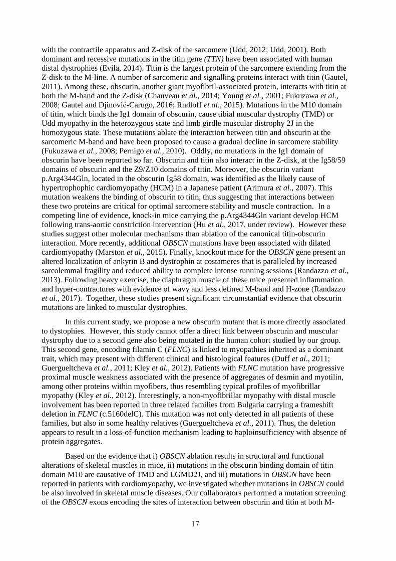
of the sarcomere (Arimura et al., 2006; Frenneaux, 2004). In HCM, there is an asymmetric

accumulation of poorly functioning, enlarged, cardiomyocytes, specifically in the left ventricle,

which results in a constricted, generally malfunctioning heart (Fig. 8; Elliot and McKenna,

Figure 7. Normal muscle (left) next to a muscle with muscular dystrophy (right). In the muscle with MD, the muscle had begun to atrophy and is smaller in mass.

11

2004; Teekakirikul et al., 2012). HCM accounts for 1% of annual mortality rates and can cause

death from sudden cardiac death, heart failure, or stroke (Frenneaux, 2004).

Obscurin mutations and pathogenesis of

muscle diseases are not as well studied as their

counterparts in titin. In fact, only a single study

involving a single example has been published

(Arimura et al., 2007). In this study, the R8 to

Q8 (Arg4344Gln) mutation in Ig58 was linked

to HCM. This mutation occurs in the OBSCN

gene in the region of that codes for the

titin/obscurin binding site and, as such, causes a

decreased binding affinity of obscurin to titin

(Arimura et al., 2007; reviewed in

Kontrogianni-Konstantopoulos et al., 2009). In

an unpublished study, a single mutation in

obscurin was linked to MD: R16 to W in Ig59

(Rossi et al., submitted).

X-Ray Crystallography

In order to understand the causes of these diseases on the molecular level, the wild-type and

mutated structures of these individual domains must be studied, elucidated, and compared. High

resolution structures of individual domains can be determined via nuclear magnetic resonance

(NMR) spectroscopy and X-ray crystallography.

X-ray crystallography first requires the growth of a single protein crystal, a periodic

assembly of protein molecules held together in a regularly-repeating lattice network by weak

molecular forces (Rupp, 2010). This can be accomplished through methods such as hanging

drop vapor diffusion, sitting drop, or microbatches (Rupp, 2010; Dessau and Modis, 2011).

Once the crystals are grown, they are harvested and kept frozen until data collection, generally

by use of a synchrotron. The structure of the repeating units within the crystal can be

determined by analyzing the diffraction of high energy electromagnetic radiation by the

electron density within the crystal lattice in the form of the crystal’s X-ray diffraction pattern.

When X-ray photons encounter these electrons, they are scattered at specific angles, whose

points or positions can be interpreted as reflections from sets of discrete lattice planes. This is

partially because the X-ray wavelength used is comparable to the interatomic distances in the

molecules studied (Wladawer et al., 2013). The angle of scattering is related to the distance

between planes h, k, and l by Bragg’s law, given below.

nλ = 2dhklsinθ

In which dhkl is the lattice plane spacing, n is the order of reflection, and θ is the scattering

angle.

The scattering function (𝑓𝑠 or 𝐹𝑠) can give the approximate X-ray scattering of an entire

system where Fs depends on the direction of scatter and, therefore, on the angle of scatter. For a

single atom, the X-ray scattering is very small and is given by:

𝐹𝑠 = ∫ 𝜌(𝑟)𝑒2𝜋𝑆𝑟𝑉(𝑎𝑡𝑜𝑚)

𝑟𝑑𝑟

Figure 8. Normal heart (left) next to a heart

with hypertrophic cardiomyopathy (right). In

the heart with HCM, the cardiac muscles

have enlarged and decreased the area

available for blood to flow.

12

In which ρ(r) is the electron density, r is the position of an electron in the atom, S is the

scattering vector— the difference between the incoming and scattered wave vectors— and

V(atom) is the volume of the atom. For a larger, repeating structure such as a molecular crystal

lattice, the scattering function is described as a sum of the scattering functions of individual

atoms:

𝐹𝑠 = ∑ 𝑓𝑠,𝑗0

𝑎𝑡𝑜𝑚𝑠

𝑗=1𝑒2𝜋𝑖𝑆𝑟𝑗

In which 𝐹𝑠 is the scattering function of the crystal and 𝑓𝑠0 is the atomic scattering factor.

The X-ray diffraction pattern can also be interpreted as transforming the crystal

structure’s electron density from real space ℝ (x, y, z) to reciprocal space ℝ* (h, k, l). In

reciprocal space, the scattering function of a molecular crystal becomes:

𝐹ℎ = ∑ 𝑓𝑠,𝑗0 𝑒2𝜋𝑖ℎ𝑥𝑗

𝑎𝑡𝑜𝑚𝑠

𝑗=1

In which 𝐹ℎ is the scattering function in terms of the index vector ℎ, 𝑥 denotes the position of

an atom/electron in an atom in fractional coordinates, and, by extension, 𝑥𝑗 denotes the position

of the 𝑗th atom/electron (Rupp). Such a transformation from real to reciprocal space is termed a

Fourier transform and can be generalized with the form:

𝐹(𝑘) = ∫ 𝐺(𝑥)𝑒2𝜋𝑖𝑘𝑥𝑑𝑥∞

−∞

a complex Fourier integral, derived as an eigenfunction of the Sturm-Liouville eigenvalue

problem with periodic boundaries (Rupp, 2010). There is an inverse relationship between the

spacing of reflections in a diffraction pattern and the spacing in the original crystal lattice,

which can be used to establish the dimensions of a unit cell within the crystal lattice (Rhodes,

2006).

The points of a diffraction pattern give the relative intensities of scattering as well as the

position. Because the structure of the unit cells of a crystal repeats periodically to form a lattice,

the incoming photon waves that scatter as a result of an electron cloud encounter each other and

can interfere constructively, destructively, or partially, resulting in an enhancement or

quenching of X-ray radiation that is depending on the direction of the wave vector (Wlodawer

et al., 2008; Wlodawer et al., 2013). These intensities are related to the complex structure factor

(𝐹) in the following way:

𝐼 = 𝐹𝐹∗ = |𝐹|2

Because F is a wave equation, it must specify the frequency, amplitude, and phase of

each diffracted ray (Rhodes, 2006). But, in calculating the amplitude of the structure factor to

gain information about the intensities of a reflection, all information about the phase angle of

each reflection is lost. This significantly encumbers the reconstruction of molecular structure,

which requires an understanding of the phases of a reflection (Rupp, 2010). The remedy to this

problem will be discussed later.

The size of the unit cell of a crystal lattice is directly proportional to the number of

diffracted beams, and, therefore, is directly proportional to the number of reflections and

reflection intensity observed. Also, due to the symmetric nature of crystals, multiple individual

measurements of intensity are expected to calculate the same, unique reflection and contribute

13

to a certain redundancy or multiplicity factor. The higher the multiplicity factor, the more

accurate the average reflection intensity, since all individual reflections have an innate degree

of random error (Wlodawer et al., 2013). The value Rmerge reports the agreement of all

symmetry-equivalent reflections that contribute to the same unique reflection and is given by:

𝑅𝑚𝑒𝑟𝑔𝑒 = ∑ ∑|< 𝐼ℎ > −𝐼ℎ,𝑖| ∑ ∑ 𝐼ℎ,𝑖

𝑖ℎ𝑖ℎ

In which h represents the unique reflections, i represents the symmetry-equivalent contributors

to each unique reflection, and < 𝐼ℎ > represents the average intensity of each reflection

(Wlodawer et al., 2013; Wlodawer et al., 2008). In other words, Rmerge compares the average

intensity of the original model with the intensity of the current model and therefore is an

indicator of bias, and, consequently, potential inaccuracies. Rmerge can also be written as:

𝑅𝑚𝑒𝑟𝑔𝑒 = ∑ ∑ |𝐼ℎ,𝑖−< 𝐼ℎ >|𝑁

𝑖=1ℎ

∑ ∑ 𝐼ℎ,𝑖𝑁𝑖=1ℎ

In which N represents all redundant measurements for each individual reflection h (Rupp,

2010). Ideally, a high-quality diffraction pattern would have an Rmerge of ≤5% (Wlodawer et

al., 2013; Wlodawer et al., 2008). However, in reality, the Rmerge may be slightly higher, though

it is generally less than 20% for large biomolecules (Rupp, 2010). Additionally, the signal to

noise ratio, < 𝐼/𝜎(𝐼) >, is defined as:

<𝐼

𝜎(𝐼)> =

1

𝑁 ∑

𝐼ℎ

𝜎(𝐼ℎ)

𝑁

ℎ

Where an acceptable range of < 𝐼/𝜎(𝐼) > is ≤1.5-2.0 (Rupp, 2010).

In short, from the diffraction pattern, it is possible to gain the positions and intensities of

individual reflection but not their phases. The inability to garner phases from diffraction data

gives rise to the ‘phase problem’ of crystallography. Phases can be supplied by other means,

such as isomorphous replacement, anomalous scattering, and molecular replacement. The

research in this thesis was conducted using molecular replacement.

Molecular replacement uses the phases and structure factors from previously solved,

similar protein structures, called phasing models, to obtain the phases of the target protein. For

example, most if not all immunoglobulin domains are comprised of very similar structures (see

Fig. 6). Therefore, it is feasible to use phases from other immunoglobulin domains to estimate

the phases of an unsolved immunoglobulin domain; generally an immunoglobulin phase model

requires a minimum of 30% sequence identity (Scapin, 2013; Chothia and Lesk, 1986). In this

case, the two structures are isomorphous, or share the same crystal structure. The electron

density, 𝜌(𝑥, 𝑦, 𝑧), of the target structure can be calculated from those of the isomorphous

phasing models by the following equation:

𝜌(𝑥, 𝑦, 𝑧) = 1

𝑉∑ ∑ ∑|𝐹ℎ,𝑘,𝑙

𝑡𝑎𝑟𝑔𝑒𝑡|𝑒−2𝜋𝑖(ℎ𝑥+𝑘𝑦+𝑙𝑧−𝛼′)

𝑙𝑘ℎ

In which V is the volume of the unit cell, 𝐹ℎ,𝑘,𝑙𝑡𝑎𝑟𝑔𝑒𝑡

is the amplitudes of the scattering function of

the target protein, 𝛼′ is the phases of the model, and the frequencies h along the x-axis, k along

the y-axis, and l along the z-axis are given by hx, ky, and lz, respectively (Rhodes, 2006). Using

the above equation, the electron density for the entire structure can be obtained giving a map of

14

the overall structure. To this, the target sequence of amino acids can be fit, giving a model of

the overall structure. Given that the first output map will be crude, because the phases of the

model are only rough estimates, both the map and model will require iterative manual and

computational improvement. However, due to the implementation of the phasing model, a great

potential for bias was also introduced— that the calculated phases from the model, rather than

the observed phases from the experimental intensities, would dominate the outputted map. To

prevent model bias, a new map can be generated by obtaining a contour in which the calculated

structure factor amplitudes (|𝐹𝑐𝑎𝑙𝑐|) are subtracted from multiple observed structure factor

amplitudes (𝑛|𝐹𝑜𝑏𝑠|):

𝜌(𝑥, 𝑦, 𝑧) = 1

𝑉∑ ∑ ∑(|𝐹𝑜| − |𝐹𝑐|𝑒−2𝜋𝑖(ℎ𝑥+𝑘𝑦+𝑙𝑧−𝛼𝑐𝑎𝑙𝑐

′ )

𝑙𝑘ℎ

In which 𝛼𝑐𝑎𝑙𝑐′ is the phases of the model. The map generated from the previous equation is

known as a 𝐹𝑜 − 𝐹𝑐 map or basic difference map and gives regions of positive and negative

densities that require moving atoms towards or away from the regions, respectively (Rhodes,

2006; Rupp, 2010). An amino acid in an unfavored conformation according to the 𝐹𝑜 − 𝐹𝑐 map

will have negative density at its current conformation and positive density nearby, where its

preferred conformation would fit.

𝐹𝑜 − 𝐹𝑐 maps rely solely on the original data and eliminate bias from the current model

so that the errors in it can be determined. Since 𝐹𝑜 − 𝐹𝑐 maps point out the errors of the current

model, it is often not useful for the beginning stages of reconstruction, when there are more

errors, because the output is ‘noisy’ and difficult to read. Therefore, a 2𝐹𝑜 − 𝐹𝑐 map or

combined difference map is more often used, which allows a greater influence from the model

but gives a more easily understood map. 2𝐹𝑜 − 𝐹𝑐 maps are given by:

𝜌(𝑥, 𝑦, 𝑧) = 1

𝑉∑ ∑ ∑(2|𝐹𝑜| − |𝐹𝑐|𝑒−2𝜋𝑖(ℎ𝑥+𝑘𝑦+𝑙𝑧−𝛼𝑐𝑎𝑙𝑐

′ )

𝑙𝑘ℎ

Through the process of model and map refinement, the particular conformation(s) of

each amino acid will be found and corrected through adjustment of variables such as clash

scores and χ and φ angles, definition of the electron density map, and decrease R-factor values,

which are defined as:

𝑅𝑓𝑎𝑐𝑡𝑜𝑟 = ∑ ∑ ∑ |𝐹𝑜𝑏𝑠 − 𝐹𝑐𝑎𝑙𝑐|𝑙𝑘ℎ

∑ ∑ ∑ 𝐹𝑜𝑏𝑠𝑙𝑘ℎ

There are a variety of R-factors, including the linear merging R value, 𝑅𝑚𝑒𝑟𝑔𝑒, defined

previously, which compares the average intensity of the original data and current model, and

the cross validation R value, 𝑅𝑓𝑟𝑒𝑒, which is calculated the same as the normal R-factor but

only for approximately 10% of the original data points. 𝑅𝑓𝑟𝑒𝑒 is given by:

𝑅𝑓𝑟𝑒𝑒 = ∑ |𝐹𝑜𝑏𝑠 − 𝑘𝐹𝑐𝑎𝑙𝑐|ℎ𝜖𝑓𝑟𝑒𝑒

∑ 𝐹𝑜𝑏𝑠ℎ𝜖𝑓𝑟𝑒𝑒

Where ℎ𝜖𝑓𝑟𝑒𝑒 denotes the excluded cross-validation set (Rupp, 2010). A high-resolution

crystal structure is defined by an 𝑅𝑓𝑟𝑒𝑒 < 20%, a resolution of 0.86–1.5 Å, and an 𝑅𝑚𝑒𝑟𝑔𝑒 <

~4%, though, practically, these values may deviate (Wlodawer et al., 2008). At this point, a

structure is considered ‘done’ and can be published.

15

In this work, the high resolution structure of obscurin Ig59 was obtained. Work is in

progress for the elucidation of high resolution structures of obscurin domains Rho-GEF, Rho-

GEF-PH, kinase I (KI), and kinase II (KII).

16

A Variant in the Obscurin Gene Associated with a Frameshift Mutation in the Filamin C

Gene in a Family with Distal Muscular Dystrophy*

*This chapter is based on a manuscript that has been submitted to PLoSONE. The writing of

this chapter was a joint effort between our lab and our collaborators in Italy.

Introduction

Distal muscular dystrophies are a group of inherited primary muscle disorders showing

progressive muscle atrophy and weakness, usually in the hands and/or feet (Mutoni and Wells,

2007; Ng et al., 2012; Sewry, 2010; Udd, 2012). These dystrophies have diverse etiologies, and

are further classified via one of four methods: i) clinical features, i.e. early or late adult onset,

onset in the hands or feet; ii) magnetic resonance imaging (MRI)-based evidence of an

involvement of the

anterior or posterior

compartment of the

legs; iii) inheritance

pattern; and/or iv)

histopathological

findings (Udd, 2012;

Mastaglia and

Laing, 1999). Here

we will use a

combination of all

four classification

schemes to describe

a new gene member

(obscurin) that

appears to be

autosomally-linked

with late onset of

distal muscular

dystrophy (see

Table 1 for a

complete list of

other genes

involved).

In contrast

with proximal

muscular

dystrophies, in

which the mutated

genes often encode

sarcolemmal

proteins, many of

the genes identified

in distal muscular

dystrophies encode

proteins associated

Type of Distal Muscular Dystropy Associated Gene

Autosomal Dominant: Late Onset

TIA1 Mutated Welander Distal Myopathy TIA1

Titin Mutated Tibial Muscular Dystropy TTN

Distal Myotilinopathy MYOT

ZASPopathy LDB3

MATR3 Mutated VCPDM MATR3

VCP Mutated Distal Myopathy VCP

aB-crystallin mutated distal Myopathy CRYAB

Thenar Atrophy with Sarcoplamic Bodies FHL1

Mutated Distal Myopathy SQSTM1

Autosomal Dominant: Adult Onset

Desminopathy DES

ABD-FLNC Mutated Distal Myopathy ABD-FLNC

DNAJB6 Mutated Distal Myopathy DNAJB6

HSPB8 Mutated Neuromyopathy HSPB8

Finnish MPD3 No known gene

Oculopharyngeal Distal Myopathy No known gene

Autosomal Dominant: Childhood Onset

Distal Myosinopathy MYH7 MYH7

KLHL9 Mutated Distal Myopathy KLHL9

Autosomal Recessive: Early Adult Onset

Miyoshi Dysferlinopathy DYSF

Distal Anoctaminopathy ANO5

GNE Myopathy GNE

Recessive Distal Titinopathy TTN

Autosomal Recessive: Childhood Onset

Distal Nebulin Myopathy NEB

ADSSL Mutated Distal Myopathy ADSSL1

Oculopathyngeal Distal Myopathy PABPN1

Table 1. Classification and genes associated with distal muscular dystrophies.

17

with the contractile apparatus and Z-disk of the sarcomere (Udd, 2012; Udd, 2001). Both

dominant and recessive mutations in the titin gene (TTN) have been associated with human

distal dystrophies (Evilä, 2014). Titin is the largest protein of the sarcomere extending from the

Z-disk to the M-line. A number of sarcomeric and signalling proteins interact with titin (Gautel,

2011). Among these, obscurin, another giant myofibril-associated protein, interacts with titin at

both the M-band and the Z-disk (Chauveau et al., 2014; Young et al., 2001; Fukuzawa et al.,

2008; Gautel and Djinović-Carugo, 2016; Rudloff et al., 2015). Mutations in the M10 domain

of titin, which binds the Ig1 domain of obscurin, cause tibial muscular dystrophy (TMD) or

Udd myopathy in the heterozygous state and limb girdle muscular distrophy 2J in the

homozygous state. These mutations ablate the interaction between titin and obscurin at the

sarcomeric M-band and have been proposed to cause a gradual decline in sarcomere stability

(Fukuzawa et al., 2008; Pernigo et al., 2010). Oddly, no mutations in the Ig1 domain of

obscurin have been reported so far. Obscurin and titin also interact in the Z-disk, at the Ig58/59

domains of obscurin and the Z9/Z10 domains of titin. Moreover, the obscurin variant

p.Arg4344Gln, located in the obscurin Ig58 domain, was identified as the likely cause of

hypertrophophic cardiomyopathy (HCM) in a Japanese patient (Arimura et al., 2007). This

mutation weakens the binding of obscurin to titin, thus suggesting that interactions between

these two proteins are critical for optimal sarcomere stability and muscle contraction. In a

competing line of evidence, knock-in mice carrying the p.Arg4344Gln variant develop HCM

following trans-aortic constriction intervention (Hu et al., 2017, under review). However these

studies suggest other molecular mechanisms than ablation of the canonical titin-obscurin

interaction. More recently, additional OBSCN mutations have been associated with dilated

cardiomyopathy (Marston et al., 2015). Finally, knockout mice for the OBSCN gene present an

altered localization of ankyrin B and dystrophin at costameres that is paralleled by increased

sarcolemmal fragility and reduced ability to complete intense running sessions (Randazzo et al.,

2013). Following heavy exercise, the diaphragm muscle of these mice presented inflammation

and hyper-contractures with evidence of wavy and less defined M-band and H-zone (Randazzo

et al., 2017). Together, these studies present significant circumstantial evidence that obscurin

mutations are linked to muscular dystrophies.

In this current study, we propose a new obscurin mutant that is more directly associated

to dystophies. However, this study cannot offer a direct link between obscurin and muscular

dystrophy due to a second gene also being mutated in the human cohort studied by our group.

This second gene, encoding filamin C (FLNC) is linked to myopathies inherited as a dominant

trait, which may present with different clinical and histological features (Duff et al., 2011;

Guergueltcheva et al., 2011; Kley et al., 2012). Patients with FLNC mutation have progressive

proximal muscle weakness associated with the presence of aggregates of desmin and myotilin,

among other proteins within myofibers, thus resembling typical profiles of myofibrillar

myopathy (Kley et al., 2012). Interestingly, a non-myofibrillar myopathy with distal muscle

involvement has been reported in three related families from Bulgaria carrying a frameshift

deletion in FLNC (c.5160delC). This mutation was not only detected in all patients of these

families, but also in some healthy relatives (Guergueltcheva et al., 2011). Thus, the deletion

appears to result in a loss-of-function mechanism leading to haploinsufficiency with absence of

protein aggregates.

Based on the evidence that i) OBSCN ablation results in structural and functional

alterations of skeletal muscles in mice, ii) mutations in the obscurin binding domain of titin

domain M10 are causative of TMD and LGMD2J, and iii) mutations in OBSCN have been

reported in patients with cardiomyopathy, we investigated whether mutations in OBSCN could

be also involved in skeletal muscle diseases. Our collaborators performed a mutation screening

of the OBSCN exons encoding the sites of interaction between obscurin and titin at both M-

18

band and Z-disk in patients affected by distal muscular dystrophy. This screening identified an

OBSCN c.13330C>T mutation, resulting in a p.Arg4444Trp substitution in the obscurin Ig59

domain. This mutation segregates with muscular dystrophy in a French family. Whole exome

sequencing (WES) of this family by our collaborators identified an additional single base

deletion in the FLNC gene (c.5161delG) causing a frameshift mutation (p.Gly1722ValfsTer61).

However, segregation analysis indicated that this FLNC mutation did not completely segregate

with the disease, as the mutation was also present in one healthy relative. These findings

resemble the results previously reported by Guergeltcheva and collaborators (Guergueltcheva et

al., 2011), where a deletion in the FLNC gene (c.5160delC) was observed in individuals with

muscular dystrophy and also in healthy individuals. WES analysis performed on the DNA from

four patients, three with the disease and one healthy, from several Bulgarian families in which

the FLNC c.5160delC was described and did not reveal any additional gene variant shared by

affected individuals. Based on our collective findings, we propose that the OBSCN

p.Arg4444Trp variant may increase the penetrance of the FLNC c.5161delG deletion in the

French family. Accordingly, variants in the OBSCN gene should be considered as potentially

causative of muscular dystrophy, alone or in association with variants in other myopathy genes.

Materials and Methods

Patient Data.† Mutation screening was initially performed in families where the affected

members presented with a clear distal myopathy phenotype transmitted as dominant trait. The

study was then extended to a cohort of 110 unrelated patients consisting of 11 cases with

predominantly proximal muscle weakness, respiratory failure and/or cardiomyopathy, 8 cases

with predominantly proximal myopathy, 26 cases with initial distal muscle involvement

subsequently progressing to proximal limb weakness, and 65 cases of patients with a clinical

history of uncharacterized muscular dystrophy/myopathy. In the French family reported here,

the proband (III:3), a woman issued from non consanguineous parents, and her second son

(IV:2), had progressive distal lower limb weakness starting at ages 30 and 14, respectively. The

proband’s father (II:2) had very late-onset walking difficulties, became wheelchair bound at age

75 and subsequently died from respiratory insufficiency and pneumonia. The paternal

grandfather (I:1) also became wheelchair-bound at an advanced age. Other family members had

no neuromuscular history. The proband and her affected son were followed in Neuromuscular

Unit of Salpêtrière Hospital (Paris, France). Among the four children of the proband, one

daughter (IV:3) and one son (IV:4), seen at the Neuromuscular Unit at age of 33 and 32,

respectively, had a normal clinical examination, with no muscle alteration as shown by MRI.

Ethics committee approval and written informed consent was obtained for all patients. This

study complies with the ethical standards stated in the 1964 Declaration of Helsinki.

Mutation Screening and Genotyping.† Mutation screening by conventional Sanger sequencing

on specific regions of OBSCN was performed in all family members for whom DNA was

available. In detail, primers were designed using Primer3 software

(http://frodo.wi.mit.edu/primer3) to amplify OBSCN exon 2 (coding for the Ig1) and exons 50,

51 and 52 (coding for the Ig58/59 domains), according to sequence NM_052843. Genomic

DNA was extracted from peripheral blood leucocytes by standard procedures (Kley et al.,

2012). Amplified DNA fragments were directly sequenced using an ABI Prism 310 apparatus

(Applied Biosystem). Alternatively, Sanger sequencing was performed using DreamTaq™

DNA Polymerase (Thermo Scientific) according to standard protocol and PCR products were

†Work of Dr. Vincenzo and collaborators

19

sequenced on an ABI3730xl DNA Analyzer (Applied Biosystems), using the Big-Dye

Terminator v3.1 kit and analyzed with Sequencher 5.0 software (Gene Codes Corporation).

DNA mutation numbering was based on cDNA reference sequence (NM_052843), taking

nucleotide +1 as the A of the ATG translation initiation codon. The mutation nomenclature

used follows that described at http://www.hgvs.org./mutnomen/.

Whole Exome Sequencing (WES).† Whole exome sequencing (WES) was performed on patients

III:3 and IV:2 at ATLAS Biolabs GmbH using SeqCap EZ Human Exome Library v2.0 (Roche

NimbleGen) for DNA capture. The enriched DNA was sequenced with an Illumina HiSeq 2000

platform, 2 x 100 bp. Reads were aligned to the human genome reference GRCh37/hg19 with

Burrows-Wheeler Aligner and duplicate reads were removed with Picard. The Genome

Analysis Toolkit was used to realign the reads, recalibrate base quality scores and call variants.

Variants were annotated using wAnnovar and variants with frequency more than 1% in the

1000 Genomes or Exome Sequencing Project (ESP6500) databases were filtered out.

Remaining variants present in both III:3 and IV:2 were analyzed.

WES on 3 patients and a normal relative from the Bulgarian families (Guergueltcheva et

al., 2011), was performed at Centro di Ricerca Interdipartimentale per le Biotecnologie

Innovative (CRIBI), Padova, Italy. DNA libraries for WES were constructed following the

standard protocol of the Ion AmpliSeq™ Exome RDY Kit (ThermoFisher Scientific). Starting

from 100 ng of gDNA, a multiplex-PCR with 12 primer pools was performed in order to allow

the amplification of 24,000 amplicons per pool, covering the exonic regions of the genomes

(about 58 Mb). 9 µl of 100 pM barcoded libraries were amplified by emulsion PCR using a

OneTouch2 instrument. Finally, the barcoded samples were loaded into Ion Proton P1 v3 chip

and sequenced on the Ion Proton instrument using the Ion Proton HiQ Sequencing kit. The

bioinformatic analysis was performed on the Ion Torrent Server and the Torrent SuiteTM was

used to base-call and align the reads to the human reference genome (GRCh37/hg19).

Alignment BAM files, Coverage Analysis statistics and Variant Analysis VCF files were

produced. By default, the variant calling was performed using the “Germ Line-High

Stringency” algorithm.

Generation of GST Expression Vectors and Constructs for in vitro Translation.† Human

OBSCN cDNA (NM_052843) coding for Ig58/59 was amplified from total RNA extracted from

human skeletal muscle tissue using specific primers (forward primer: 5’- aagaacacggtggtgcggg

– 3’; reverse primer: 5’- gaggcccagcagggtgagc-3’). The OBSCN cDNA containing the

c.13330C>T variant was generated by PCR using primers designed to introduce the cytosine to

thymine nucleotide change into the wild-type cDNA (forward primer: 5’-

aacgcggcggtcTgggccggcgcacag – 3’; reverse primer: 5’- ctgtgcgccggcccAgaccgccgcgtt-3’) and

sequenced using an ABI Prism 310 apparatus (Applied Biosystems). The amplified sequences

were cloned into the vector pGEX (GE Healthcare) using the EcoRI-SalI sites to generate GST-

OBSCNWT and GST-OBSCNMUT fusion proteins. Human TTN cDNA (NM_001267550) was

amplified from total RNA extracted from human skeletal muscle tissue using specific primers.

The TTN cDNA containing the Z9/Z10 domains of TTN was generated by PCR using the

following primers (forward primer: 5’ - gacaaagagaaacaacagaaa – 3’; reverse primer: 5’ –

atcttccctctgttgaatctc – 3’) and sequenced using an ABI Prism 310 apparatus (Applied

Biosystems). The amplified sequences were cloned into the vector pGBK-T7 in frame with a

myc tag epitope (Clontech) using the EcoRI-SalI sites.

†Work of Dr. Vincenzo and collaborators

20

Protein Expression and in vitro Interaction Studies.† GST fusion proteins grown in Escherichia

coli (E. coli) (BL21(DE3)) were induced at OD600=0.6 with 1 mM isopropyl β–D-

thiogalactopyranoside (IPTG) for 3 hrs at 30°C. Cells were harvested centrifugation at 4000 xg

for 10 min at 4°C. The pellet was resuspended in cold buffer containing Phosphate Buffer

Saline (PBS), 1% Triton X-100, 20 mM EDTA and lysed by sonication on ice. The soluble

fraction was obtained by centrifugation at 13200 xg for 15 min at 4°C. The fusion proteins were

immobilized by incubating 1 ml of the soluble fraction with 100 µl of glutathione-Sepharose 4B

resin (GE Healthcare, Buckinghamshire, United Kingdom) for 10 min and washed three times

with 1 ml of a buffer containing PBS and 1% Triton X-100 (Rossi et al., 2014a). Beads were

finally resuspended with an equal volume of PBS and the protein was eluted from the column

with glutathione-PBS buffer.

In vitro translation and transcription experiments were performed using the TNT Quick

Coupled Reticulocyte Lysate System as described by the manufacturer (Promega). 5 µl of the

translation reaction were incubated with 12 µg of GST fusion protein in a buffer containing 10

mM Tris-HCl pH 7.9, 150 mM NaCl, 0.5% NONIDET P-40, 1 mM DL-Dithiothreitol (DTT), 1

mM phenylmethylsulfonyl fluoride (PMSF) and protein inhibitor mixture for 1.5 hrs at 4° C.

After incubation, the GST fusion protein complexes were washed 3 times with interaction

buffer. Bound proteins were eluted by boiling in sodium dodecyl sulfate polyacrylamide gel

electrophoresis (SDS-PAGE) sample buffer and analysed by SDS-PAGE.

Western Blot Analysis. Protein samples were separated by 10% SDS-PAGE. Filters were

incubated with primary antibody (mouse anti-c-myc, Clontech-Zymed Laboratories Inc.), and

diluted in blocking buffer overnight at 4°C with agitation. Filters were washed three times with

washing buffer (0.5% non-fat dry milk, 50 mM Tris-HCl pH 7.4, 150 mM NaCl, 0.2% Tween-

20) for 10 min each, incubated with horseradish peroxidase-conjugated secondary antibody and

detected using the ECL system (ECL Western Blot Detection Reagents, Promega).

Nuclear Magnetic Resonance (NMR) Preparation and Data Collection. All chemicals were

ACS grade or higher and were typically purchased from Fisher Scientific unless otherwise

specified. Recombinant 15N, 15N-13C, and unlabeled protein were purified after overexpression

in BL21 cells using a pET24a vector system (Novagen, San Diego CA) in a manner similar to

(Rossi et al., 2014b). All nuclear magnetic resonance (NMR) experiments were collected on a

600 MHz Bruker Avance II spectrometer equipped with a TXI room temperature 5 mm probe

with z-axis pulse field gradient coils. All NMR samples were collected at 25 C in 20 mM Tris

pH 7.5, 20 mM NaCl, 0.35 mM NaN3, and 0.5-2.5 mM protein with 10% D2O. All 2D and 3D

NMR experiments were collected as previously described (Rossi et al., 2014b). Further

description of NMR collection is located in the supplemental information. Chemical shifts for

Ig59 have been deposited in the Biological Magnetic Resonance Bank (BMRB) under

accession number 26593.

A 2D HSQC was collected, as well as standard triple resonance experiments including

HNCACB, CBCA(CO)NH, HNCO, HN(CA)CO, C(CO)NH, H(CCCO)NH, 15N-edited

TOCSY, 15N-edited NOESY, 13C-edited NOESY, and pseudo-3D IPAP experiment for H-N

residual dipolar couplings, as previously described (Rudloff et al., 2015). Both NOESY

experiments used 110 ms mixing time. Most experiments were collected with 128, 64 and 1024

points in the T1, T2, and T3 dimensions, respectively. NMR data were processed with

NMRPipe (Muntoni, 2007), extended in the indirect dimension via linear prediction, and the

resulting spectra were analyzed via Sparky (Lee et al., 2015).

Standard Bruker IPAP experiments using 256 points for each T1 dimension were used

to collect RDC data in isotropic and axially-compressed 5.5% acrylamide gel samples, as

†Work of Dr. Vincenzo and collaborators

21

previously described (Ng et al., 2012). The program PALES was used for RDC alignment

tensor fitting with a calculated Aa and Ar component of 0.00163 and 0.000901, respectively

(Sewry, 2010). For all experiments, the 1H chemical shifts were referenced to external DSS, the

13C shifts were referenced indirectly to DSS using the frequency ratio 13C/1H = 0.251449527

and 15N shifts were referenced indirectly to liquid ammonia using 15N/1H = 0.101329118.

NMR Structure Calculation. Interproton distance constraints were derived from 3D NOESY

experiments (15N-edited and 13C-edited 3D NOESY) as described previously. Dihedral

constraints ± 20˚ and ψ ± 15˚ for -helix and ± 40˚ and ψ ± 40˚ for -sheet were included

based on TALOS+ and the chemical shift index of 1H and 13C atoms (Rudloff et al., 2015).

Residual dipolar coupling data was included based on splitting values from an IPAP

experiment, as previously described (Shen et al., 2009). More information about the structure

calculations can be found in the supplemental information. The final 20 structures were selected

(from 200) based on lowest Q-values and lowest root mean squared deviation (RMSD) from the

average, and were of high quality based on the statistical criteria listed in supplemental Table 3.

The coordinates of the human OBSCN Ig59 structure have been deposited in the Protein Data

Bank (2N56).

An ensemble of structures without dihedral restraints had a backbone RMSD of 0.85 Å

when compared to structures with dihedral constraints (Udd, 2012). We attempted to further

verify the structure by performing a H-D exchange experiment, however this Ig domain

remains unfolded after lyophilization. Therefore, hydrogen bond constraints were not tested

directly but instead were added into the structure only after the secondary structure was

completely determined. Structures calculated without hydrogen bonds had an RMSD of 0.59 Å

when compared to those calculated with hydrogen bonds, indicating that inclusion of these

bonds did not drastically influence the overall structure. Hydrogen bond constraints of rHN-O =

1.5 Å to 2.8 Å and rN-O = 2.4 Å to 3.5 Å were included in the final stage of structure

calculations, and were based off regions that were clearly in well-defined secondary structural

motifs. Pseudopotentials for secondary 13Cα and 13Cβ chemical shifts and a conformational

database potential were included in the final simulated annealing structural calculations using

the computer program XPLOR-NIH (Mastaglia and Laing, 1999; Udd and Griggs, 2001).

Structures run with and without these pseudopotentials show an RMSD of 0.58 Å. The

internuclear dipolar coupling (in Hz) were determined from the difference in J splitting between

isotropic and radially compressed polyacrylamide, and were incorporated into the final

structure calculation as previously described using an energy constant of 0.50 (Evilä et al.,

2014; Gautel, 2011). A comparison of structures run with and without RDC measurements

show an RMSD of 0.67 Å. Q-factors were calculated by randomly removing ≈ 10% of the N-

HN RDC data, and then comparing these values to those back-calculated from the structure.

Purification of Obscurin Ig59. Protein samples of pet-24a(+) human obscurin Ig59 were

expressed in E. coli and purified through the following procedure. Starter cultures (~5mL) of

Ig59 were made following addition of glycerol stock (500ul Ig59 PEP24A BL-21 cells into

50/50 glycerol) and 10ul of kanamycin. Starter cultures were shaken overnight at 37C, 250rpm,

then added to 1L flasks of Luria broth (LB) (10g tryptone, 5g yeast extract, 5g NaCl, dilute to

volume with diH2O) along with 1mL kanamycin. These flasks were also shaken at 37C,

250rpm. Induction occurred ~3hr later, at 0.6-0.8 OD, with the addition of 0.2g IPTG.

Approximately 3hr later, flasks were taken out of the incubator/shakers and centrifuged using a

JLA 16.250 rotor at 6000rpm, 4°C for 15min. The supernatant and pellet were separated and

the pellet was kept at -80°C until ready for further purification. Pellets were resuspended in

G75 buffer (20 mM Trist, 50 mM NaCl, azide) and 100ul PMSF was added to prevent

degradation during sonication at 100% amplification, 15s pulse, for 30min, then centrifuged

†Work of Dr. Vincenzo and collaborators

22

using a JA 25.50 rotor at 14000rpm, 4°C for 30min. The supernatant was run over a Nickel

column and the eluent was concentrated in a 5K concentrator tube via centrifugation at

4500rpm for 90min intervals until less than 1mL solution remained, then run over a size

exclusion column. Contents of column fractions were visualized using gel electrophoresis;

fractions containing Ig59 were pooled and concentrated. The concentration of Ig59 in the

resulting solution was obtained using a Thermo Scientific Nanodrop 2000 Spectrophotometer

using the extinction coefficient (12490 cm-1M-1) and molecular weight (11.1 kDa) of Ig59.

Crystallization and X-ray Diffraction. The hanging drop method with 17% tacsimate, 0.1M

HEPES pH 7.5, 4%

PEG3350, and 10 mg/mL

protein was used to obtain

Ig59 crystals. Crystals were

harvested and frozen in

liquid nitrogen after one

week using a glucose

cryoprotectant and

crystallographic reflections

were collected at the

Structural Biology Center

beamline 19-ID-D at the

Advanced Photon Source,

Argonne National

Laboratory. HKL2000 data

processing calculated the

unit cell to be P 31 2 1

(Otwinosky and Minor,

1997).

Structure refinement.

Crystal diffraction phasing

was determined using the

program Phaser-MR in the

PHENIX ver 1.72.2-869

program suite via molecular

replacement using PDB and

reflection files from

accession numbers 2YZ8

and 4RSV. The resulting

structure was refined using

the program PHENIX ver.

1.72.2-869-refine (Afonine

et al., 2012). COOT was

used to manually rebuild the

structure in iterative rounds

of rebuilding and refinement

in PHENIX refine, resulting

in a 1.18 Å resolution

structure with an Rfree value

of 0.185 (Emsley et al.,

2010). More refinement

Wavelength (Å) 0.97918

Resolution range (Å) 30.49 - 1.177 (1.219 - 1.177)

Space group P 31 2 1

Unit cell (Å) 60.98 60.98 47.56 90 90 120

Unit cell (°) 90 90 120

Total reflections 662701 (35265)

Unique reflections 33764 (3303)

Multiplicity 19.5 (10.7)

Completeness (%) 98.82 (92.53)

Mean I/sigma(I) 22.98 (5.07)

Wilson B-factor 14.83

R-merge 0.1345 (0.5394)

R-meas 0.1389

CC1/2 0.988 (0.912)

CC* 0.997 (0.977)

R-work 0.1642 (0.2634)

R-free 0.1851 (0.2974)

Number of non-hydrogen

atoms

775

macromolecules 678

ligands 0

water 97

Protein residues 90

RMS(bonds) 0.033

RMS(angles) 1.46

Ramachandran favored (%) 99

Ramachandran outliers (%) 0

Clashscore 2.23

Average B-factor 20.5

macromolecules 19.4

ligands 0

solvent 28.3

Table 2. Final refinement statistics of human obscurin domain Ig59.

Parentheses indicate the statistics of the outer shell.

23

statistics are given in Table 2. The coordinates of Ig59 have been deposited in the PDB under

accession number 5TZM.

Molecular Dynamics Modelling. Coordinates corresponding to the crystal structure of Ig59

were allowed to equilibrate using YASARA 12.7.16, at 310K, 150 mmol/L NaCl, pH 7.4, using

the Amber ff03 forcefield in a simulation cell with periodic boundaries until the backbone

RMSD no longer changed significantly (Wright et al., 2005). Simulations were run with a

timestep of 1.25 fs with the temperature adjusted using a Berendsen thermostat as described by

Krieger et al. (Krieger et al., 2014; Kireger et al., 2004). Once finished, the p.Arg4444Trp

mutation was introduced to the simulation using the ‘swap’ function in YASARA. This mutated

structure was then once again allowed to equilibrate using the same parameters as for the wild-

type structure, and the simulation was terminated when the RMSD stabilized. YASARA and

Pymol were used to visualize the structures (de Groot et al., 1997; The PyMOL Molecular

Graphics System).

Circular Dichroism. All CD experiments were conducted in a 1 mm pathlength cuvette at 15

μM protein in 20 mM Tris buffer, pH 7.5 and 100 mM NaCl. Samples were measured in

triplicate at 37°C on a Jasco J-810 spectrophotometer.

Results

Clinical Findings. † Our collaborators performed quantitative studies on human patients with

dystrophies in order to investigate the disease. The proband (III:3) of these studies was a 61-

year-old female presenting a progressive distal dystrophy since around age 30, affecting

successively the right hand and progressing slowly to include both distal upper and lower limbs.

At age 45, difficulties in standing up from a chair and a steppage gait appeared. At age 51,

ambulation was not limited, but the patient exhibited foot drop (more pronounced on the right

side), inabilities to stand on tip toes or heels, and a waddling gait. Hand finger extensors, foot

evertors, toe extensors, and calf muscles showed severe weakness, but finger flexors and the

tibialis anterior were normal. Glutei maximi, thigh adductors, and hamstrings were also

severely affected, but proximal scapular, brachial, and antebrachial involvement was not

detected. Hand palmar muscles (mainly thenar ones), calves and tibial muscles were atrophic

(Fig. 1A1-5). In addition to the worsening myopathy, a progressive cervical myelitis of

unknown aetiology appeared at age 52, manifesting as a sensory defect mainly in left lower

limbs and spreading from foot to hip, causing severe pains and impaired balance. At age 61, she

could walk slowly a few hundred meters with two aids. The previously described clinical

selective pattern was found with severe wasting of hand finger extensors, toes extensors,

peroneus lateralis, posterior calf muscles, and hamstrings. Hand finger flexors, tibialis anterior,

quadriceps, along with scapular, brachial, antebrachial, axial, facial and oculo-bulbar muscles

remained mostly spared. Quantitative measurements are detailed in Table 3. A sensory defect

due to the myelopathy was found in both distal and proximal lower limbs (left > right). Creatine

kinase (CK) levels were normal. Electromyogram (EMG) showed myopathic changes distally

in the upper limbs and both proximally and distally in the lower limbs. Cardiac evaluation

(ECG and echocardiography) and spirometry were normal. Spinal cord MRI performed at age

53 revealed a posterior hyperdense signal from C2 to C7 (Fig. 1-C2-C7). Brain MRI and CSF

were normal.

†Work of Dr. Vincenzo and collaborators

24

Our collaborators reported that the proband’s son (IV:2) noticed first symptoms

(fatigability in walking and difficulties in standing on tip toe) at age 14. He has been unable to

run since the age of 16 years. He could walk a distance of around 1000 meters without aid at

age 33. He had marked weakness and atrophy in the calf muscles and minor weakness in the

interossei and finger extensors, but otherwise normal muscle strength in the proximal lower

limbs and in the upper limbs (Table 3). No facial or bulbar weakness was present. CK levels,

spirometry and cardiac evaluation were normal. Electromyography (EMG) showed myopathic

changes.

25

Table 3. Quantitative clinical measurements performed by our collaborators documenting the progressive muscular dystrophy of the proband and her son. Case

Age

Sex

Symptom

onset

(age in years)

Course

Current status: (age)

functional ability

Current status

Muscle weakness

Current status

Muscle atrophy

CPK/ EMG / Cardiac

echography/ EKG/ Vital

capacity

Case I

Proband

61y

F

Right hand

atrophy /

weakness

(finger

extensors)

(≈ 30y)

Progressive worsening

Around 30y : both hands

wasting, inability to stand on

heels and tiptoes, 35 y

difficulties climbing stairs.

46 y Gowers, difficulties standing

from a chair, running inability.

Increased weakness of foot

evertors, hand finger extensors

52y : cervical myelitis

manifesting by left foot

extending to whole limb after 6

months. sensory defect without

identified cause (Spine MRI T2

sequence hypersignal from C2 to

C7)

(normal Brain MRI, normal CSF

fluid)

Increased loss of balance and

cordonnal pains

53 y : fallings (weakness and

balance impairment)

59 y : walk with bilateral aid

(61y)

Walking distance : few

hundreds meters with aid

Fallings, four to five

times monthly

right foot elevator

Difficult walk with

steppage and tendency to

internal rotation of feet

10 m in 15 s with a cane.

Inability to stand on heels

and tiptoes

Rising from chair 9 times

in 60 s with two hands

Thigh crossing : difficult

Arm elevation : normal

Painful spinal posterior

column syndrome

(myelitis)

Lower limbs Toes extensors 2, except big toe,

1 , Peroneus 1, , Tibialis anterior

4, Post legs 2+ Hamstrings 2,

Quadriceps 5-

Adductors 2+, Glutei maximi

2+, Glutei medii 4+, Iliopsoas 4+

Upper limbs

Finger extensors 3-, index more

affected :

right index 2, left 2+

Finger flexors 4+

wrist extensors 4

scapular and brachial 5

Axial and neck flexors 4-

facial, oculobulbar normal

in addition : hypoesthesia of

whole left lower limb due to

myelitis

Legs (both

compartments)

Hand : palmar,

mostly thenar

region

CK normal

EMG : myogenic

Distal in Lower limbs, Distal +

proximal in lower limbs

Nerve : normal

No decrement

Normal echography and EKG

VC : 85%

Case II

Son of

case I

33 y

M

Difficulties

standing on

tiptoes and

heels

fatigability in

walking

(14y)

Mild progression

At 16 y, interruption of sport at

school and inability to run.

(33y)

Walking distance : 1000

m without aid

No fallings

Climbing stairs with

banister 10 m : 12s

Rising from a chair : 24

times in 60 s without aid

Arm elevation : normal

Lower limbs Peroneus 3-, Tibialis anterior 3+

Toes extensors between 4 , and 2

(big toe) Post legs 2

Pelvic and femoral muscles 5

Upper limbs

Finger extensors 4+,

Finger flexors 5

wrist extensors 5

scapular and brachial 5

Axial and neck flexors 5

facial, oculobulbar normal

Legs, mainly

posterior

compartment

No atrophy of

upper limbs

CK normal

EMG : diffuse myogenic

pattern

Nerve : normal

Normal echography and EKG

VC : 86%

26

Muscle imaging performed by our collaborators on the mother at the age of 51 showed

severe fatty degenerative changes in almost all lower leg muscles, except for tibialis anterior,

posterior and long toe flexor muscles. The quadriceps was considerably less affected than the

hamstrings and adductors. Glutei maximi and iliopsoas were less affected than glutei minimi and

medii. The forearm extensor

muscles showed reduced volume.

At age of 61 years, this pattern

remained mostly unchanged,

except that the vastus medialis and

vastus internalis fatty degeneration

was more marked, particularly in

right side. Rectus femoris and

vastus lateralis remained spared

(Fig. 1). In the 33-year-old son, the

changes in CT scan were milder,

with the exception of severe fatty

replacement in the calf muscles

and, less severely, in the lateral

compartment peroneal muscles. All

other muscles were intact.

The radialis muscle biopsy

from the proband (III:3) performed

at 51 years showed some nuclear

internalization, fiber size variation

(Fig. 1B1), and type 1

predominance. Oxidative

histoenzymatic reactions disclosed

few lobulated fibers and uneven

staining of the intermyofibrillar

network (Fig. 1-B2). Our

collaborators’ peroneal muscle

biopsy of the son (IV:2) at 33 years

showed marked fiber size

variability with the presence of

some atrophic angulated fibers (Fig.

1C1). A few lobulated fibers were

also present.

Immunohistochemistry performed

in both muscle biopsies revealed

some desmin surcharge in both

patients (Fig. 1B3, C2). In contrast

only patient IV:2 (the son of the

proband) harboured alphaB

crystallin immunoreactive

aggregates (Fig. 1C4). Myotilin

immunostaining did not show

Figure 1. A/B) Clinical data, C) morphological studies, and

D) ultrastructutal studies of the proband (III:3). A1-3:

Evidence of muscle atrophy in thenar muscles. A4-5: All

distal leg muscles of the proband are markedly affected,

except for tibialis muscles. B1-4: Computed Tomography

(CT) of the proband at the age of 51 showed severe fatty

degeneration changes in most leg muscles. C1-C4: Radialis

muscle biopsy of proband (III:3). C1. Haematoxylin & Eosin:

presence of some nuclear internalization and fiber size

variation. C2 NADH: lobulated fibers are indicated by an

arrow; uneven staining of the intermyofibrillar network in

some fibers is indicated by a star. C3 desmin: mild diffuse

desmin surcharge in several fibers C4 myotilin.:ormal

staining. C5-C8: Peroneal muscle biopsy from the proband

son (IV:2). C5 NADH: atrophic lobulated fibers are indicated

by an arrow. C6 desmin: mild diffuse desmin surcharge in

several fibers. C7 alpha B cristallin: presence of dense

protein aggregates. C4 myotilin: normal staining. D. Radialis

muscle biopsy of proband (III:3), EM analysis. D1: presence

of numerous abnormal mitochondria harbouring dotty or

paracrystallin inclusions, in proximity of the star. D2:

presence of a cytoplasmic protein aggregate composed by

dark osmiophilic granulo-filamentous material corresponding

to desmin, indicated by an arrow, and filamentous material

indicated by an asterisk.

27

specific alterations (Fig. 1B4, C4). Ultrastructural studies performed by our collaborators on the

proband (III:3) showed myofibrillar disorganizations resembling targetoid structures in a small

percentage of the fibers (not shown). Abnormal mitochondria with some paracristalline

inclusions (Fig. 1B5, indicated by a star) and dark dots were observed in numerous fibers. Focal

disintegration of myofibrils, dark osmiophilic granulo-filamentous material corresponding to

desmin (Fig. 1C5, indicated by an arrow) and filamentous protein aggregates (Fig. 1C5,

indicated by an asterisk) were observed in PX (or son of the proband).

However, a

subsequent WES

analysis,

performed by our

collaborators

using the DNA

from the III:3

proband,

identified an

additional novel

frameshift

mutation in the

FLNC gene

(NM_001458.4).

This was a

deletion of a

single base in

exon 30

(c.5161delG)

resulting in a

frameshift and a

premature stop

codon

(p.Gly1722Valfs

Ter61, Fig. 2B).

Sanger

sequencing for

FLNC exon 30

was performed

by our

collaborators on

II:1, III:3, III:4,

IV:1, IV:2 and

IV:3. The FLNC

variant

c.5161delG was

present in the

two affected individuals (III:3, IV:2) but also in one healthy individual (IV:3). This deletion is

located adjacent to the previously reported c.5160delC deletion, which is linked to distal

Figure 2. Genetic analysis of OBSCN c.13330 C>T and FLNC c.5161delG mutations. A) Family pedigree. Black filled symbols represent affected family members. The genotype of individuals is shown as follows: +/+ wild type, OBSCN +/- heterozygous for the c.13330 C>T mutation, FLNC +/- heterozygous for the c.5161delG mutation. Arrow indicates the proband. B) Electropherogram of the OBSCN gene sequence (upper panel) and of the FLNC gene sequence (lower panel). C) Phylogenetic alignment of the OBSCN orthologs. Sequences represent the Ig59 domains of OBSCN in distinct mammalian species. The arginine in position 4444 in the human OBSCN sequence is highlighted in yellow and is conserved in mammalian species. D) Interaction between titin domains Z9/Z10 and OBSCN domains Ig58/Ig59. in vitro transcribed and translated myc-tagged titin domains Z9/Z10 were used in pull-down experiments with GST-fusion proteins containing either wild type OBSCN Ig58/Ig59 domains (OBSCNWT) or R4444W mutated OBSCN Ig58/Ig59 domains (OBSCNMUT). Proteins were separated by SDS-PAGE, transferred to membranes and detected by mouse anti-myc antibodies. E) Quantification of GST pull-down efficiency. Protein bands intensities of myc-tagged Z9/Z10 titin domains precipitated by either OBSCNWT or OBSCNMUT GST-fusion proteins were evaluated by densitometric analysis and normalized on GST fusion proteins content. Data represent means values ± standard deviation of five independent experiments in triplicate. * p < 0.01 following t-test statistical analysis.

28

myopathy with upper limb predominance in three Bulgarian families (Guergueltcheva et al.,

2011). To investigate if the OBSCN variant identified in the French family was present also in

the Bulgarian families with recurrence of the FLNC c.5160delC frameshift, our collaborators

initially performed Sanger sequencing of exons 2, 50, 51 and 52 of the OBSCN gene in 12

individuals from the three related Bulgarian families [3 unaffected non-carriers of the FLNC

c.5160delC (2701:IV.1, 2702:III.3; 2703:IV.3), 4 asymptomatic carriers of the FLNC c.5160delC

(2701:IV16; 2701:V1; 2701:V2; 2702:IV3), and 5 individuals with distal dystrophy carrying the

FLNC c.5160delC(2701:IV3; 2701:IV.10; 2702:III.1; 2702:IV.1; 2703:III.2)]. Since this initial

screening did not identify any variant in the selected exons of OBSCN, WES analysis was

performed by our collaborators in three affected FLNC mutation carriers and one normal relative

from the Bulgarian families (patients IV:3 of family 1, III:1 of family 2, III:2 of family 3 and

individual IV:1 of family 1) Variants were filtered for a global minor allele frequency ≤0.001,

shared by the affected individuals but not present in the asymptomatic member. This analysis

identified no mutation (missense, nonsense, indel) shared by the patients and not present in the

normal relative of the Bulgarian families.

Structural Studies of the Ig59 Domain of OBSCN. From the above analysis, we reasoned that the

dual OBSCN and FLNC mutations may represent a digenic heterozygous condition, where the

OBSCN mutation leads to an increased penetrance of the FLNC mutation. In order to begin

defining the molecular mechanism of the described phenotype, we investigated how the normal

and mutated obscurin Ig59 domain interacts with its binding partner titin. We first solved the

high-resolution structure of Ig59 (residues 4428-4521). Human obscurin Ig59 was isolated based

on the original sequence alignment (CAC44768.1) (Young et al., 2001). After purification, the

beta-sheet rich structure was verified by CD, the pure Ig59 was crystallized. The resulting

crystals diffracted to a resolution of 1.18 Å (Fig. 3A, Table 2). The resulting structure shows beta

sheets extending from Glu 4435 to Lys 4438 (strand A’), Ala 4440 to Arg 4443 (strand A), Ala

4446 to Thr 4453 (strand B), Ser 4464 to Ile 4468 (strand C), Trp 4479 to Asp 4484 (stand D),

His 4487 to

Leu 4493

(strand E),

Gly 4501 to

Ala 4506

(stand F),

and Ala

4512 to Leu

4519

(strand G).

Overall, the

structure

forms a

typical Ig-

like fold

(Meyer and

Wright,

2013).

Figure 3: Structure and analysis of human obscurin Ig59. A) Cartoon of the Ig59 crystal structure, showing the typical Ig-like fold. B) Comparison between the Ig59 NMR and X-ray structure. C) CD plot of WT obscurin Ig58-59 (black squares) and p.Arg4444Trp (open circles). D) MD simulated average models of WT (blue) and Arg4444Trp (red) Cα positions. The side chains for Arg4444/Trp4444 are shown. E) RMSD vs residue number comparison of the mutant model to the wild-type model. The Arg444Trp site is shown in red.

29

An independently solved NMR solution structure of human obscurin Ig59 contains

greater than 12 restraints per residue (Fig. 3B, Fig. 4, Table 4). The overall backbone root mean

squared deviation (RMSD) of ordered heavy atoms is 0.609 Å. With the exception of Arg 4430,

and Arg 4508, every backbone H-N bond and most sidechain C-H shifts are visible in these

NMR experiments. H-N residual dipolar coupling experiment values independently verify the

validity of this

structure, and result

in a Q-factor of 0.25

±0.02. The NMR

and X-ray structure

have a pairwise

RMSD of 1.609 Å

(Fig. 3B). The

differences between

the two structures

are most

pronounced

between residues

Asn 4468 and Ser

4478. This area is in

a long loop region,

and is associated

with higher B-

factors in the X-ray

structure and a

lower number of

NOE restraints in

the NMR structures.

Aside from this

area, the structures

are highly similar to

each other.

Figure 4. NMR data used to determine the structure of human obscurin Ig59. A) Observed beta sheet interactions of Ig59 as seen in the 15N-edited NOESY. B) NOESY data (in black) overlaid with TOCSY data (in red), showing self-peaks and cross-strand NOEs. C) Example of CBCA(CO)NH (in red) and HNCACB (in black) experiments, showing NMR assignments. D) Example of residual dipolar coupling data showing isotropic (right) and anisotropic (left) examples of the H-N bond from A78.

30

Table 4. NMR-derived statistics of 20 NMR structures1 of human obscurin domain Ig59. Parenthesis indicate the number of restraints.

The

p.Arg4444Trp mutation

could affect the obscurin-

titin interaction in two

ways: it may unfold the

entire Ig59 domain, or it

may maintain the fold

and simply perturb the

binding event. To

examine the effect of the

p.Arg4444Trp mutation

on the Ig59 structure, we

conducted circular

dichroism (CD)

experiments on the WT

and mutant forms of Ig59.

As can be seen in Fig.

3C, the CD profiles are

virtually identical,

suggesting that the

mutation does not

globally disrupt the

overall Ig-like

architecture. To gain

greater insight into the

local effect of the

p.Arg4444Trp, the WT

and mutant protein

structures were examined

using molecular

dynamics (MD). In each

case, the RMSD relative

to the starting model was

measured until the

simulation was fully

equilibrated. The resulting models of wild-type and p.Arg4444Trp were then compared (Fig. 3D,

E). While the long flexible loop between residues 4468 and 4478 was significantly different

between these simulations, regions around the mutation were virtually unchanged in structure.

Thus, these in silico results are consistent with our CD work showing that the mutation does not

change the Ig59 structure significantly. Therefore, the p.Arg4444Trp variant likely directly alters

the obscurin-titin interface.

1 The 20 ensemble structures, <20>, are the results of simulated annealing calculations. The best structure is the closest to the average structure. The values shown for the <20> are the mean ± standard deviation.

<20> Best

RMSD from distance

constraints (Å)2

total (1061) 0.028 ± 0.002 0.029

intraresidue (228) 0.005 ± 0.004 0.003

sequential ( |i – j| = 1) (382) 0.019 ± 0.005 0.022

medium range ( 1 < |i – j| ≤

1) (95)

0.046 ± 0.006 0.056

long range ( |i – j| = 1) (292) 0.031 ± 0.003 0.003

hydrogen bonds (64) 0.056 ± 0.006 0.050

RMSD from exptl dihedral

constraints (°)

Φ,Ψ (144) 0.687 ± 0.116 0.684

RMSD from dipolar

coupling restraints (Hz)

DNH (52) 0.89 ± 0.09 0.93

RMSD from exptl 13C

chemical shifts

13Ca (ppm) 1.59 ± 0.17 1.31

13Cb (ppm) 1.46 ± 0.04 1.47

RMSD from idealized

geometry

bonds (Å) 0.004 ± 0.001 0.004

angles (°) 0.633 ± 0.020 0.640

impropers (°) 0.442 ± 0.036 0.431

Lennard-Jones potential

energy (kcal/mol)3

-363 ± 10 -359

Q-value4 0.27 ± 0.04 0.25

% most favorable region in

the Ramachandran plot5

74.1± 3.0 72.8

RMSD of the mean

structure (Å)6

all backbone atoms (3-91) 0.609 ± 0.063 0.494

all heavy atoms (3-91) 1.2128 ± 0.080 1.157

31

2 None of the 20 structures has a distance violation > 0.35 Å or a dihedral angle violation of > 5°. The force constants used in the SA calculations are as follows: 1000 kcal mol −1 Å2 for bond length, 500 kcal mol−1 rad−2 for angles and improper torsions, 4 kcal mol−1 Å−4 for the quartic van der Waals (vdw) repulsion term (hard-sphere effective vdw set to 0.8 times their values in CHARMm parameters), 50 kcal mole−1 Å−2 for experimental distance constraints, 1 kcal mol−1 Å−2 for distance symmetry constraints, 0.5 kcal mol−1 ppm−2 for the 13C chemical shift constraints, and 1.0 for the conformational database potential. The force constants (in kcal Hz−2) used for dipolar coupling restraints is 0.50. 3 Lennard-Jones van der Waals energies were calculated using CHARMm parameters and were not used in any stage of the structure determination 4 Q-values were determined by randomly removing 10% of all RDC values. To ensure accuracy, an ensemble of structures with a second randomly removed subset of RDCs was also run. The Q-value of this second set was similar to the first. 5 PROCHECK was utilized to generate the Ramachandran plot 6 Backbone calculations include Cα, N, and C′ atoms. Only residues 3–91 are included since no long-range NOE correlations were observed for residues 1–2 and 92–104.

The p.Arg4444Trp Variant Reduces the Interaction between Obscurin Ig58/59 and Titin Z9/Z10

Domains. To directly evaluate whether the p.Arg4444Trp variant alters the interaction of the

Ig58/59 domains of obscurin with the Z9/Z10 domains of titin, we performed GST-pull down

assays with either immobilized GST-obscurinWT or GST-obscurinMUT mixed with in vitro-

translated titin Z9/Z10, cloned in frame with a myc-tag epitope. Densitometric quantification of

the binding between the Z9/Z10 domains of titin and the Ig58/59 domains of obscurin showed

that the bound fraction of GST-obscurinWT protein was approximately two-fold higher than that

of the GST-obscurinMUT, indicating that the p.Arg4444Trp variant significantly weakens the

titin-obscurin interaction (Fig. 2D, 2E). Other groups have suggested that this titin-obscurin

interaction helps to strengthen the Z-line (Bang et al., 2001). Our results show that the

p.Arg4444Trp variant leads to a partial ablation of titin binding. This event leads to a weaker,

less organized cytoskeleton, which in turn contributes to the distal muscular dystrophy

phenotype of affected patients. This general mechanism of action is similar to the titin M10

mutations found in TMD and LGMD2J patients, which also serve to ablate a separate titin-

obscurin interaction.

Discussion

Based on the evidence that the M10 domain of titin is mutated in patients with TMD and

LGMD2J and that this domain interacts with the Ig1 domain of obscurin (Fukuzawa et al., 2008;

Pernigo et al., 2010), we hypothesized with our collaborators that the OBSCN gene could

represent a potential candidate for those cases of muscular dystrophies where a causative gene

had not been identified. Screening performed by our collaborators of families with undetermined

distal myopathy led to the identification of a novel variant in OBSCN, p.Arg4444Trp, which co-

segregated with a c.5161delG in FLNC, in two individuals of a French family affected by distal

muscular dystrophy. The OBSCN p.Arg4444Trp variant is conserved across mammalian species

and is localized in a region of the protein that mediates the binding to the Z9/Z10 Ig domains of

titin which facilitates the localization of obscurin to the Z disk region of the sarcomere (Young et

al., 2001).

32

Our structural studies showed that the previously mentioned variant does not lead to a

global Ig59 domain misfolding but instead changes the surface topology of the domain. This

mutation may thus affect obscurin binding to other members of the myofibril cytoskeleton. Pull-

down experiments showed that this variant specifically weakens the binding between obscurin

and titin, which may contribute to altered sarcomere stability and, eventually, disease. In support

of this hypothesis, other mutations have been identified in patients with muscular dystrophies

that affect the titin-obscurin interaction. For instance, mutations in the titin M10 domain, which

mediates interaction with the Ig1 domain of obscurin at the M-band, were found to reduce the

affinity of titin for obscurin and cause gradual failure of sarcomere maintenance in muscles of

patients affected by TMD and LGMD2J (Fukuzawa et al., 2008; Pernigo et al., 2010). Similarly,

the p.Arg4344Gln variant located in the Ig58 domain of obscurin identified in a patient affected

by hypertrophic cardiomyopathy, was found to impair the binding of obscurin to the Z9/Z10 Ig

domains of titin (Arimura et al., 2007). Moreover, knock-in mice for the p.Arg4344Gln variant,

when exposed to stress via trans-aortic constriction, develop a severe cardiac hypertrophy within

4-8 weeks (Hu et al., 2016), further emphasizing the complementary roles of titin and obscurin in

maintenance of sarcomere stability.

Interestingly, the two variants of Ig58 and Ig59 mentioned in this text, p.Arg4444Trp of

Ig59 and p.Arg4344Gln of Ig58, involve a single point mutation from a charged to an uncharged

residue (Arimura et al., 2007; Fukuzawa et al., 2008; Guergueltcheva et al., 2011; Pernigo et al.,

2010). The isoelectric points of these regions are approximately 6.34 and 4.16, respectively.

However, the point mutations cause a shift in isoelectric point to 4.48 and 3.90, respectively.

Therefore, we hypothesize that the binding events between Ig58/59 of obscurin and Z9/10 of titin

is electrostatically driven and that the difference pIs account for the reduction in binding affinity

observed in the variants. In the future, we will test this hypothesis by creating a titin column and

testing its affinity for the obscurin wild types and variants. If a lower concentration of salt is

required to wash off the variant compared to the wild type, then we can effectively conclude that

the variant affinity is lowered due to a decrease in electrostatic interactions.

FLNC mutations are known to cause adult-onset distal muscular dystrophy (Kley et al.,

2012; Vorgerd et al., 2005; Shatunov et al., 2009; Luan et al., 2010). The protein product of

FLNC, filamin C, is an actin cross-linking protein involved in cytoskeleton organization and

signalling (Razinia et al., 2012). Mutations in FLNC were reported to destabilize muscle tissue

homeostasis via the formation of protein aggregates (Löwe et al., 2007). In addition, mutations in

FLNC have been detected in patients with myofibrillar myopathy and also in patients with hand

muscular dystrophy without myofibrillar aggregates (Duff et al., 2011; Guergueltcheva et al.,

2011).

Our collaborators’ clinical evaluations of the proband carrying both the OBSCN

p.Arg4444Trp variant and the FLNC deletion indicate a late-onset dominant distal muscle

dystrophy as well as the involvement of additional muscle groups than the Udd Myopathy (Duff

et al., 2011; Guergueltcheva et al., 2011). The FLNC mutation did not completely segregate with

the disease, as it was present in the two affected patients as well as one healthy individual in the

French family analyzed. This incomplete segregation matches the behavior of a similar FLNC

deletion reported in Bulgarian families (Guergueltcheva et al., 2011), indicating an incomplete

penetrance of the genotype. WES of representative individuals in the Bulgarian families did not

reveal the presence of any other gene variants shared by all patients. Thus, the genetics behind

the incomplete penetrance of the disease in the Bulgarian families remains unsolved and,

33

therefore, needs further analysis. In the French family reported by our collaborators, the

combination of the FLNC c.5161delG frameshift and the OBSCN c.13330C>T variant co-

segregated with the disease, with the OBSCN variant present only in the affected individuals. The

healthy relative presenting only the FLNC c.5161delG deletion can be regarded as partial

asymptomatic carrier.

In conclusion, the data on the French family reported by our collaborators depicts a novel

digenic heterozygosity condition in the genetics of distal dystrophy, resulting in a dominant

phenotype with quite severe clinical features; individual III:3 was unable to walk and constricted

to a wheelchair, and IV:2 was unable to run since the age of 16. This phenotype is caused

partially by an altered titin-obscurin interaction, and partially by altered filament C function of

unknown molecular etiology.

34

Studies on the Molecular Motion, Structure, and Elasticity of Titin

Introduction

Titin’s ability to both stretch and recoil is fundamental in preventing muscle

overstretching and helps myocytes return to their original length. Recent studies have examined

titin’s mechanosensing abilities using tandem Ig and Fn-III-like domains (Granzier and Labiet,

2004; Linke et al., 2008; von Castelmur et al., 2008; Lee et al., 2010; Pernigo et al., 2010; Hsin

et al., 2011). While many of these domains are closely associated with other parts of the

cytoskeleton, there are ~100 tandem domains in the sarcomeric I-band that are relatively free

from extensive target protein interactions (reviewed in Kontrogianni-Konstantopoulos et al.,

2009). Improta et al. (1998) and von Castelmur et al. (2008) have shown that this I-band region

acts as a modified entropic spring whereby each domain behaves as a link in a chain connected

by 3-5 residue interdomain linker ‘hinges’ (Improta et al., 1998; von Castelmur et al., 2008)

(Fig. 1).

The further a

polypeptide is stretched,

the more energy

additional stretching

requires (Linke, 2000

(1);Linke, 2000 (2)).

Through extensive

molecular dynamics

(MD) simulations, Lee et

al. took this idea further

and developed a

comprehensive

mathematical model

where tandem Ig domains

behave as a kind of

entropic-enthalpic spring,

termed the ‘modified

worm-like model’

(mWLM) (Lee et al.,

2007; Hsin et al., 2011). In this model, the Ig domains can move stochastically relative to one

another, though there is also some breaking and forming of transient domain-domain and

domain-linker non-covalent bonds. The mWLM agrees extremely well with the experimental

data and explains titin’s stretch resistance at very low forces (1-5 pN) (Linke, 2000 (1); Ma and

Wang, 2003; Hsin et al., 2011). At slightly higher forces (~5 pN), the mainly disordered PEVK,

N2A, and N2B regions of titin straighten out in an entropic-enthalpic spring mechanism

(Frieburg et al., 2000; Bang et al., 2001; Ma and Wang, 2001; Ma and Wang, 2003; Li et al.,

2002; Lee et al., 2007). At extremely high forces (>50 pN), discrete titin Ig and Fn-III domains

completely unfold, although the physiological relevance of such an event is uncertain (Rief et al.,

2000; Li et al., 2003; Garcia et al., 2009; Stacklies et al., 2009; Lee et al., 2010; Hsin et al.,

Figure 1. Short linker regions of I6 between A) Ig66-67, B) Ig67-68, and C) Ig69-70.

35

2011). Thus, titin displays a continuum of soft elasticity with the application of force (Hsin et al.,

2011).

This nuanced view of titin’s flexibility at low forces runs somewhat counter to the crystal

structure of 6 tandem titin domains, I65-70 (I6), which depict well-formed interactions between

the linker regions and Ig domains (von Castelmur et al., 2008). Such fixed interdomain

interactions lead to the ‘carpenter’s ruler’ model. This model reconciles several incongruences

that arise from thinking of titin as a worm-like model: data collected by cryo-EM show large

segments of the I-band region to be in straight lines with only occasional bend points, and SAXS

data indicate a mostly elongated structure (Marino et al., 2006; Vazina et al., 2006; von

Castelmur et al., 2008; Marchetti et al., 2011). Additionally, the persistence length of the titin I-

band region is longer than a worm-like model would suggest (Di Cola et al., 2005; von

Castelmur et al., 2008).

In an attempt to resolve the discrepancy between the worm-like and ‘carpenter’s ruler’

models, we re-analyzed the published crystal structure data (von Castelmur et al., 2008; Lee et

al., 2007). Many of the linker/domain interactions that are present in the original model and

contribute to an elongated overall structure are either absent or ambiguous in our structure (Fig.

1). Examination of symmetry mates suggest that the extended conformation of titin is not based

on stabilizing domain-linker interactions but based instead on crystal packing interactions.

Molecular dynamics simulations performed by others and ourselves support the theory

that this region of titin can be elongated, however the energy difference between a slightly bent

and a straight molecule are below the threshold of thermal noise (Lee et al., 2010). Together,

these X-ray and MD analyses structurally validate the mWLM. Titin likely forms transient

interdomain interactions, which explains the protein’s resistance to stretch and its persistence

length. These interactions, combined with limited flexibility due to steric hindrance between Ig

domains, serve to keep titin in a mostly elongated orientation. While there is computational and

circumstantial evidence for stabilizing interdomain interactions (Matsubara and Maruyama,

1977), their presence in this crystal structure is not definite.

Materials and Methods

Structure Refinement. PDB and reflection files from accession numbers 3B43 and 2RIK

were implemented in experimentation. The structure of 3B43 was refined computationally and

manually using PHENIX ver 1.72.2-869 and Coot was used for iterative rounds of structure

rebuilding and refinement in PHENIX refine (Terwilliger et al., 2008). Amino acids with

continuous, clearly defined electron density at 𝜎 ≥ 1.5 for at least two residues were included;

all others were excluded. Ramachandran outliers were identified using the Molprobity server and

Coot. Once identified, outliers were corrected. Refinement statistics are given in Table 1 (Chen

et al., 2010; Emsley et al., 2010). The 2RIK structure was used for investigation of crystal

packing interactions and the possible effects of packing on rigidity.

36

Table 1. I6 statistics after refinement. Methods for data collection of I6 are found in von Castelmur et al., 2008.

Molecular

Dynamics

Simulations. All

MD simulations

were performed

with the PMEMD

module of the

Amber 12 MD

software package,

the AMBER 12SB

force field, and a

generalized Born

implicit solvent

(Hornak et al.,

2006; Case et al.,

2012; Nguyen et al.,

2013). The non-

bonded interaction

cutoff distances

were set at 100 Å

for MD and 150 Å

for steered molecular dynamics (SMD). For equilibrium simulations, constant temperature (T =

300K) was enforced using a Langevin thermostat with a collision frequency of 1 ps-1. The

integration time step was 2 fs and all covalent bonds to hydrogen were held fixed with the

SHAKE algorithm.

Steered Molecular Dynamics Simulations. SMD simulations fixed the α-carbon at the N-

terminus of Ig65 (A1) and applied force to the α-carbon at the C-terminus of Ig70 (Q567),

moving it closer to the N-terminus (Israleqitz et al., 2001). In this way the protein was

compressed at a constant velocity of 15 Å/ns. The SMD spring constant was set at 10 (kcal mol-1

Å-2).

Results

The original structure of I65-I70 is hook-shaped; the first two domains are oriented 114

degrees relative to the final four domains, which are nearly linear (von Castelmur et al., 2008).

The high B factors of the published structure prompted our re-analysis of the electron density in

3B43 to determine if the sections with high B-factors had well-defined electron density. A 1.5 σ

cutoff was used to fit the model in Coot. Continuous, unambiguous density for the backbone and

side chains was required; all other residues and side chains were removed (Table 1 for fitting

statistics and Fig. 2A). This newly refined structure has an RMSD of 0.6 Å compared to the

original with several important differences. The overall B-factor is significantly lower than the

original structure (88.4 Å3 vs 118.5 Å3; Fig. 2A inset). Furthermore, domain Ig68 is almost

completely absent. In our model, interactions between the Ig domains and linker residues, which

Resolution range (Å) 16.99-3.30

Spacegroup P6522

Unit cell dimensions a=b=141.43Å, c=166.01Å

α=β=90°, γ=120°

Solvent content (%) 67.1

Matthews coefficient 3.74

Completeness (%) 98.6

Refinement:

No. of reflections 14953

No. of protein atoms in asymmetric unit 3371

R factor/R free (%) 28.4/31.0

RMSD bond length (Å) .0084

RMSD bond angle (°) 1.992

Avg B factor (B factor range) (Å3) 88.5 (19.9-200.2)

Wilson B factor (Å3) 82.6

Ramachandran favored (%) 90.6

Ramachandran outliers (%) 2.2

37

were previously postulated to stabilize the structure in an elongated form, are either poorly

defined or absent (Fig. 2B). These residues were removed due to poor electron density (see

Materials and Methods for details). Analysis of the entire structure reveals a positive correlation

between extensive crystal packing interactions and low B-factors (Fig. 2A and C; Fig. 3).

From this

analysis, we

reasoned that the

overall shape of this

region of titin could

be explained by

crystal packing

interactions and not

through inter-

protein interactions

(Fig. 2D). Since

titin is predicted to

be moderately

flexible, this

hypothesis could

explain the

dichotomy between

MD simulations and

the crystal

structures. We

therefore

investigated the

structure of Ig68-

69-70 (2RIK),

which was

previously solved at

1.6 Å resolution to

determine if crystal

packing may have

also contributed to

its extended

conformation (von

Castelmur et al.,

2008). As can be

seen in Fig. 2E,

this construct has

extensive packing

interactions against its neighbors, and has correspondingly lower overall B-factors. Overlays of

the same domain in 2RIK and 3B43 show that, while the tertiary structure of the Ig domains are

virtually identical, the orientation of the Ig domains relative to each other vary (Fig. 4). We

conclude that the overall shape of I6 observed in the 3B43 crystal structure is most likely

dependent on crystal packing, not inter-protein domain-domain or domain-linker interactions.

Figure 2. A) Cartoon representation of Ig65-70, colored by B-factor. Inset is the distribution of B-factors within the model. B) Linker region between Ig67 and Ig68, showing a lack of interactions and electron density to keep the molecule rigid. C) Example of the extensive packing of Ig66 against its symmetry mate, denoted with *. D) Global view of the crystal packing of Ig65-Ig70 relative to symmetry mates. E) Global view of the crystal packing of the 2RIK structure with central molecule colored via B-factors (range from 20-65 Å3).

38

To examine

the flexibility of titin

Ig65-Ig70, we

performed a series

of MD and SMD

simulations on the

original titin

structure. Model

equilibration using

implicit solvent

conditions and the

AMBER ff12SB

force field showed

that each domain

displayed significant

motions relative to

its neighbor over 10 ns (Fig. 5). This is despite the Ig domains themselves being essentially static

(average RMSD per domain over 10 ns is about 1.9 Å). This result agrees with similar

experiments performed by Lee et al. (Lee et al., 2010). To further probe the stiffness of this

section, we brought

together the two ends of

this structure together at a

rate of 15 Å/ns, from 232

Å to 141 Å. Analyses

show that the straight part

of the original structure

(Ig67-Ig70) bent readily

and that it required less

than 0.6 kcal/mol of work

(a rough cut-off for noise

attributable to random

thermal motion) to

decrease the end-to-end

distance to 200 Å (Fig.

6A-C). Smaller-diameter

models required progressively more work. These data suggest that while the last 4 domains are

mobile relative to their neighbors, mobility only extends to roughly 140 degrees as measured

from the center of mass from each domain, in agreement with previous data (Lee et al., 2010). At

smaller angles, these Ig domains begin to run in to each other; thus, this molecule is intrinsically

partially elongated. These data agree well with previously published MD bending data, as well as

experimental SAXS data, showing that the average length of the I6 region is 220 Å (von

Castelmur et al., 2008; Lee et al., 2010).

Figure 3. Crystal packing between A) Ig69 and B) Ig70 and their respective symmetry mates (denoted with *).

Figure 4. Alignment of Ig68 between the 2RIK (cyan) and 3B43 (green) structure, showing that the neighboring Ig domains are in different orientations between the two structures.

39

Discussion

Here we re-analyze the Ig65-

Ig70 crystal structure and

suggest that the X-ray data do

not support the ‘carpenter’s

ruler' model of titin in solution.

Instead, these data agree with

subsequent MD simulations

showing that titin domains

move mostly independently of

each other, with only transient

inter-domain or domain-linker

interactions (Lee et al., 2010;

Hsin et al., 2011). This is

particularly evident in Ig68,

whose dynamic movement

makes it virtually invisible in

the structure. The presence of

motion in this region is likely

caused by a lack of symmetry

mates to pack against, resulting

in higher-than-average B-

factors.

Our new model of Ig65-70 does not explain EM data that indicate that this region of titin

is mostly elongated (von Castelmur et al., 2008). Several possibilities could explain this

discrepancy. First, it could be that transient interdomain and domain-linker interactions, while

weak, short-lived, and not present in the crystal structure, are present in sufficient quantities as to

exert a substantial stabilizing force on the molecule. These interactions could be overwhelmed by

thermal motion and crystal packing interactions and might not be seen in crystal structures. Such

interactions are built into the mWLM and seem to fit the wet lab stretching data (Lee et al., 2010;

Hsin et al., 2011). Previous SMD experiments had problems in explicit solvent with

hydrodynamic drag (Lee et al., 2010). Thus, another possible explanation is that titin, once

straight, tends to stay straight because of insurmountable solvent drag. Lastly, it may be that in

the conditions under which EM experiments were conducted, titin is particularly amenable to

forming straight lines.

Figure 5. Snapshots of MD simulations for I6 at A) 2 ns, B) 5 ns, and C) 9 ns of equilibration, showing the straightening and bending of the final four domains. The models were aligned from residue 98 to 288.

40

MD simulations argue for a

mWLM, yet previous a crystallography

structure suggest a more rigid molecule.

In this work, we identify crystal-packing

artifacts as contributing to the apparent

rigidity of the published crystal

structure. Thus, the crystallography data

in fact also suggest a dynamic system.

This more nuanced view of the X-ray

data reconciles this structure with the

subsequent MD simulations.

Figure 6. A) Force (in kcal/mol) v. distance (Å) graph of Ig65-70 (PDB 3B43). Images of Ig65-70 at B) 0 and C) 33 Å of compression.

41

Insight into the Auto-inhibitory Mechanism of the Second Kinase Domain of Obscurin

Introduction

Obscurin isoform B is expressed in low levels in a wide variety of non-muscle tissues,

including epithelial, brain, liver, pancreas, and kidney tissues (Ackermann et al., 2014; Russell et

al., 2002; Stroka et al., 2016). This isoform of obscurin is unique in that it has two

serine/threonine kinase domains located near its C-terminus (Russell et al., 2002). Interestingly,

these kinase domains are the only direct signaling moieties in obscurin. Obscurin also contains a

RhoGEF/PH tandem domain that activates RhoA. All of these three obscurin regions— the two

kinase domains and the RhoGEF/PH tandem domain— are involved in cell adhesion and

signaling. The obscurin kinase domains phosphorylate cadherins while the activation of RhoA

causes downstream effects that influence integrin signaling (Hu and Kontrogianni-

Konstantopoulos, 2013; Stroka et al., 2016). Ultimately, the cellular consequences of these

signals are increased cell adhesion and stress fiber formation.

Obscurin is normally associated with cytoskeleton stability and dynamics. Thus, these

three obscurin signaling domains provide a strong link between the cytoskeleton and cell

adhesion. Ablation of this link has considerable (but little-studied) physiological repercussions—

obscurin is the second-most mutated gene in breast and colorectal cancers (Wood et al., 2007;

Sjoblom et al., 2006; Stroka et al., 2016). Additionally, while non-tumorous tissue is rich in

obscurin, biopsies of human breast cancer tumors have shown that obscurin is nearly absent in

cancerous tissues (Stroka et al., 2016). Due to these findings, it is paramount to understand the

mechanism of action of these signaling domains and how mutations affect the activation,

expression, and/or functionality of obscurin.

The overall goal of this project is to obtain high-resolution crystal structures of both

human obscurin kinases, KI and KII. However, this goal has run into several significant hurdles.

KI does not express well. KII can be expressed, purified and crystallized, but this process is

extremely inefficient— protocols recovered an average of 1 mg from 16L of bacterial culture.

Therefore, in lieu of a crystal structure, we opted to model the KII domain using computer

simulations. Although the obscurin kinase domains have not been well-studied, the structure and

mechanism of activation of a similar kinase, the titin kinase, has been extensively studied

(Mayans et al., 1998; Mayans et al., 2013). Like all kinase domains, the titin and obscurin

kinases have two active sites that neighbor each other: a substrate binding site and an ATP-

binding site. These sites

undergo cycles of activity and

inhibition, depending on the

needs of the cell, and as such,

have highly specific

regulatory and substrate

recognition mechanisms

(Mayans et al., 1998).

The titin and obscurin

kinases are serine/threonine

kinases; they phosphorylate

Figure 1. Schematic showing the similarity between titin (left) and obscurin (right) kinase regions. All three kinases are preceded by an Ig domain (green), the titin kinase and KI are also preceded by an Fn-III domain (grey), and all three domains have an N-terminal tail (NL, yellow) and C-terminal tail (CL) in obscurin or C-terminal regulatory domain (CRD) in titin (red) (adapted after Hu and Kontrogianno-Konstantopoulos, 2013).

42

serine and threonine residues. The two domains have similar surrounding are modular and are

linked to the rest of the molecule through a (presumably) unstructured N-terminal and C-terminal

linkers (NL and CL, respectively) (Hu and Kontrogianno-Konstantopoulos, 2013; Mayans et al.,

2013) (Fig. 1). These domains are catalytically active; they can both auto-inhibit and auto-

activate themselves (Mayans et al., 1998; Hu and Kontrogianno-Konstantopoulos, 2013) (Fig. 2).

This function is a hallmark of most kinases (Tsai and Nussinov, 2013).

In the context of the entire protein architecture, the obscurin domains mirror titin (Fig. 1).

Preceding the titin kinase are an Ig domain, an Fn-III (Fn-3) domain, and the N-terminal tail

(NL). Following the titin kinase are the C-terminal regulatory tail (CRD) and another Ig domain.

Similarly, in obscurin, the first kinase is preceded by an Ig domain and NL, followed by the CL.

The second kinase domain region is also similar in its organization; as it is preceded by an Ig

domain, Fn-III domain, and NL, and immediately followed by its CL (Fig. 1). The CL is at the

extreme C-terminus of obscurin and, therefore, there is no possibility of an Ig domain following

the CL.

The titin kinase

is usually inactive; structural

studies have shown that the

CRD wraps around the kinase

domain and occludes the ATP-

binding pocket. In addition, the

N-terminal region of the titin

kinase can also bind at or near

the active site. Together, these

domains prevent ATP-binding.

(Hu et al, 1994; Kobe et al.,

1996; Mayans et al., 1998;

Gold et al., 2006) (Fig. 3).

The titin kinase

domain’s unusual auto-

inhibitory structure hints at its

mechanism of action. Titin

acts like a molecular spring;

when stretched, the

mechanical stretch physically

removes the NL and CRD

from the titin active site,

freeing it for substrate- and

ATP-binding (Grater et al.,

2005; Puchner et al., 2008;

Puchner and Gaub, 2010;

Stahl et al., 2011). The NL

and CRD binding each

effectively halves the catalytic

activity and, therefore, the phosphorylation levels of the titin kinase. Together, the NL and CRD

silence phosphorylation levels completely (Johnson et al., 2001; Masterona et al., 2011). This

Figure 2. Gel depicting the auto-phosphorylating nature of obscurin KII as well as its ability to phosphorylate cadherins (taken from Hu and Kontrogianni-Konstantopoulos, 2013).

Figure 3. Lateral and frontal surface views of titin kinase showing the inhibited conformation. Note the position of the NL (yellow) and CRD (red) in relation to the active site, Δ (taken from Mayans et al., 2013).

43

mechanism is the only known mechanism of how the cytoskeleton directly acts as a

mechanosensor- titin stretch results in target phosphorylation through the release of this auto-

inhibitory mechanism.

Given that obscurin and titin have a similar overall architecture, perform similar

connecting functions within the cytoskeleton, and contain similar kinase domains, we

hypothesize that the kinase domains also are stretch-activated mechanosensors. As a first step to

testing this hypothesis, we must determine whether the NL and CL regions of the obscurin kinase

domains interact with the kinase domains. Towards this beginning goal, we took a two-pronged

approach. To further investigate the auto-inhibitory mechanism of KII, the recombinant domain

was purified and crystallized. From these crystals, the high-resolution crystal structure KII will

be solved, though work is still in progress. Parallel to this wet-lab work, we also study computer

simulations of KII. Herein, I describe the binding affinity studies performed on a simulated

model of KII obtained by using titin’s kinase as a model structure. The data indicate that,

although the N-terminal tail of KII cannot bind to the active, site, the C-terminal domain appears

to bind.

Materials and Methods

Purification of Obscurin KII. Protein samples derived from a pet-24a(+) construct containing a

codon-optimized human obscurin KII domain were expressed in E. coli and purified as follows:

Starter cultures (~5mL) of KII were made following addition of glycerol stock (500 μl KII

pET24a BL-21 cells into 50/50 glycerol) and 10 μl of kanamycin. Starter cultures were shaken

overnight at 37°C, 250 rpm, then added to 1 L flasks of LB (10 g tryptone, 5 g yeast extract, 5 g

NaCl, in 1L dH2O), along with 1 mL kanamycin. These flasks were shaken at 37°C, 250 rpm.

Induction occurred ~3 hours later, at 0.6-0.8 OD600, with the addition of 0.2 g isopropyl β-D-1-

thiogalactopyranoside (IPTG). Approximately 3 hours later, flasks were taken out of the

incubator/shakers and centrifuged using a JLA 16.250 rotor at 6000 rpm, 4°C for 15 min. The

supernatant and pellet were separated and the pellet was kept at -80°C until ready for further

purification. Pellets were resuspended in His-tag binding buffer ((50 mM NaH2PO4, pH 8.0, 0.3

M NaCl, 100mM imidazole)) and 100 μl phenylmethane sulfonyl fluoride or

phenylmethylsulfonyl fluoride (PMSF) was added to prevent degradation during sonication at

100% amplification, 15 s pulse, for 30 min, then centrifuged using a JA 25.50 rotor at 14000

rpm, 4°C, for 30 min. The resulting pellet underwent two cycles of 8 M urea resuspension and

centrifugation under the same conditions as described previously. PMSF (100 μl) was added to

the resulting supernatant, which was then dialyzed in a buffer containing 50 mM NaCl and 20

mM Tris pH 7.5 at 4°C for 2-3 hours. This solution was centrifuged again using a JA 25.50 rotor

at 14000 rpm, 4°C for 30 min, then the supernatant was run over a Nickel column. The eluent

was concentrated in a 5K concentrator tube via centrifugation at 4500 rpm, 4°C for 90 min

intervals until less than 1 mL solution remained, then run over a size exclusion column. Contents

of column fractions were visualized using gel electrophoresis; fractions containing KII were

pooled and concentrated. The concentration of KII in the resulting solution was obtained using a

Thermo Scientific Nanodrop 2000 Spectrophotometer using the extinction coefficient (42330

cm-1mol-1) and molecular weight (30.3 kDa) of KII.

44

Crystallization. The hanging drop method with various crystallizing solutions was used to obtain

KII crystals. Crystals were harvested and frozen in liquid nitrogen until X-ray diffraction

analysis using a glucose cryoprotectant.

Model Creation and Verification. The sequence of KII was modeled using PHYRE homology

modeling. Verification of the model was performed in YASARA under explicit solvent

conditions for ~15 ns (Krieger et al., 2014; Krieger et al., 2004). The N-terminal and C-terminal

tails were not modeled using PHYRE as they were predicted to be relatively unstructured

regions.

Active Site Determination. Active residues in KII were determined via COACH analysis

protein/ligand binding site prediction meta-server (Yang et al., 2013) (Fig. 4).

N-terminal Binding Affinity Tests. The NL was modeled by hand as a random coil in YASARA

and allowed to equilibrate for ~10 ns (Krieger et al., 2014; Krieger et al., 2004). The N-terminal

tail and KII domain were the run through HADDOCK2.2 web docking prediction interface

server (van Zundert et al., 2016). Ligand 1 was KII, with active residues as predicted by COACH

and ligand 2 was the N-terminal tail.

C-terminal Binding Affinity Tests. The CL of KII was modeled by taking the PHYRE model and

fusing it to the C-terminal regulatory domain of titin. The titin sequence was then swapped out

and replaced with the obscurin KII sequence. The CL and KII domain were the run through

HADDOCK2.2 web docking prediction interface server (van Zundert et al., 2016). Ligand 1 was

KII, with active residues as predicted by COACH. Ligand 2 was the CL. Five runs were run in

total with each run marking a different active segment of the CL. Runs were structured to run 10

CL residues as active with each sequential run overlapping by four residues. For the purposes of

these tests, only the first 26 residues of the CL were tested; the CL wraps almost entirely around

the main chain of KII and it would be nearly impossible for the residues directly behind the

catalytic core to bind.

Figure 4. Sequence of KII showing active residues (magenta), NL (yellow), and CL (red). Sequence of KII obtained from PubMed obscurin isoform B, where numbers to the left indicate the residue number in the obscurin isoform.

45

Results

The obscurin KII model was made using the PHYRE homology program with the titin

kinase as a template (Fig. 5A). The original PHYRE-based model is seen in Fig. 5B. To verify

the stability of this model, the model was equilibrated for 15 ns in explicit solvent at 310K using

YASARA. At this point, no

significant conformation

changes were observed and the

ATP-binding pocket remained

intact (Fig. 6). The average

structure and last structure,

shown overlaid in Figure 5,

have an RMSD of 1.436.

Therefore, this equilibrated

model was deemed of

sufficient quality to move

forward with binding affinity

simulations.

Following structure

validation, the N-terminal tail

was modeled by hand using the add residue function in YASARA. This procedure was chosen

due to the small size of the NL; it is only 20 residues and is not predicted to have any regular

secondary structure. Therefore, a random coil, allowed to equilibrate in solution, was a good

starting point for initial binding studies. The NL and

KII were then sent through a HADDOCK prediction

binding web server to determine the likelihood of

binding between the N-terminal tail and the active site

of KII. HADDOCK is an information-driven flexible

docking approach that predicts binding energies from

predicted protein interfaces using ambiguous

interaction restraints. Thus, this is an off-shoot of other

ab initio binding algorithms. As an output,

HADDOCK primarily uses a Z-score. This number

represents the separation from the mean of all clusters

tested. Thus, the lower the Z-score, the better a certain

target docks into the protein binding site, as measured

against a random insertion event (van Zundert et al.,

2016).

While the RMSD for NL binding to KII is large, the overall Z-score is moderately good,

suggesting that the NL can bind to the kinase domain. However, close examination of the

structure reveal that these models require the removal of a critical beta strand in the kinase

domain in order to bind. Given that this strand is a central part of the kinase domain, we suspect

that this binding event would not occur in reality. HADDOCK runs with this beta strand intact

demonstrate poor binding. (Fig. 7A-C). Similar results were obtained with an increased size in

the KII binding pocket, indicating that even a large binding area did not improve NL binding. In

Figure 5. A) Cartoon representation of titin kinase showing the (yellow), CRD (red), and active residues (taken from PDB). B) Model of KII showing active residues (magenta), CL (red), and NL (yellow).

Figure 6. Average (green) and last (cyan) structures obtained from the YASARA verification of the KII model during ~15 ns of equilibration in explicit solvent.

46

total, these data strongly suggest that, despite its close proximity, the N-terminus does not

substantially interact with the KII active site (Fig. 7A-C).

Although the

N-terminal tail

could not bind to

KII’s active site,

this would not

necessarily be the

case for the CL.

This tail is longer

than the N-terminus

at 44 residues. This

long region

precluded modeling

by hand. Since this

tail may act similar

to the titin domain,

the CL sequence

was threaded

through the titin

CRD Structure. As

the CL begins on

the opposite side of

the molecule from

the active site, only

the end of this

stretch was tested.

Proximal residues

would be to far

away to bind to the

active site.

We tested

this binding in two

ways. First, we

threaded the

obscurin C-

terminal domain

through the titin

CRD region and

docked this onto

our obscurin KII

model. We then let

this region

equilibrate in

explicit solvent

Figure 8. A) Model of KII (cyan) and C-terminal tail (red). B) HADDOCK results for the test of KII ATP-binding site with residues 4-14 of the CL showing Z-score vs RMSD showing small, stable RMSD between the two structures. The structure shown in A is Cluster 2, displayed by blue triangles in the plot.

Figure 7. A) Model of KII (cyan) with all β-strands intact. The NL not shown to more clearly see all five β-strands. B) Model of KII (cyan) and NL (yellow) after the fifth β-strand was removed. C) HADDOCK results of Z-score vs RMSD showing large, variable RMSD between the two structures. The structure shown in B is Cluster 23, displayed by black triangles in the plot.

47

using YASARA for 50 ns. Analysis from this simulation indicated multiple regions of the

obscurin CL could bind to our KII model. Next, we took overlapping sequences of the KII CL

and performed HADDOCK runs into the KII active site, in a similar way to how we tested the N-

terminal region. In total, 5 separate KII/CL runs were completed, each considering 9 possible

clusters. Consecutive runs differed in the ‘active’ region of the CL, beginning with the first ten

residues and overlapping by 4 residues each time. In other words, residues 1-10, 4-14, 8-18, 12-

22, and 16-26 were run separately. HADDOCK results consistently predicted binding between

the CL and KII’s active site with low RMSDs and reasonable Z-scores (generally >-1.7) (Fig. 8).

The run in Figure 8 considered the ATP-binding site and residues 4-14 of the CL as active and

shows cluster 2 from the 4-14 run. The interactions between the NL and active site tended to be

electrostatic interactions.

Discussion

HADDOCK analysis determined that the NL was able to bind to the active site of KII but

only if there was significant displacement of the fifth β-strand, which is unlikely due to the

extensive hydrogen-bonding amongst β-sheets. Binding occurred via electrostatic interactions

between the KII active site and NL when this fifth β-strand was removed. Consistent binding was

observed between the CL and the active site, as shown by HADDOCK analysis. This binding

occurred electrostatically between the ATP-binding site of KII and the CL and is presumably

similar in nature to that of the CRD binding to the ATP-binding site of the titin kinase. However,

the in vivo and in vitro validity of the obscurin KII/CL binding event has yet to be tested. If the

binding is relatively strong, then it is likely that the CL has some inhibitory nature on the active

site. If not, then KII must be auto-activated and auto-inhibited by some other mechanism. Given

that not all proteins in the titin-like family are activated in the same manner as each other, nor as

titin itself (Mayans et al., 2013; Greene et al., 2008), coupled with our findings regarding the NL

and KII, this possibility may be even more likely as the possibility that obscurin and titin kinases

hold similar mechanisms of activation.

In the future, we hope to quantify the strength of the KII/CL binding using YASARA to

determine how much force is required to break the electrostatic bond between the two structures.

To complement this computer research with wet-lab work, we will design and implement an

affinity column to test the affinity of the CL for the kinase domain as well as the ability of the

CL to displace substrate and/or ATP from the active site(s) of KII. Lastly, we will continue to

crystallize KII in order to solve its crystal structure.

48

Appendix A: Methods for Additional Projects

Materials and Methods (KI)

Purification of Obscurin KI. Protein samples of pet-24a(+) human obscurin KI were expressed in

E. coli and purified through the following procedure. Pet-24a(+) KI was transformed onto BL-21

cells and starter cultures (~5mL) of KI were made from these with the addition of 10ul of

kanamycin. Starter cultures were shaken overnight at 37C, 250rpm, then added to 1L flasks of

LB (10g tryptone, 5g yeast extract, 5g NaCl, dilute to volume with diH2O), along with 1mL

kanamycin. These flasks were also shaken at 37C, 250rpm. Induction occurred ~3hr later, at 0.6-

0.8 OD, with the addition of 0.2g IPTG. Approximately 3hr later, flasks were taken out of the

incubator/shakers and centrifuged using a JLA 16.250 rotor at 6000rpm, 4C for 15min. The

supernatant and pellet were separated and the pellet was kept at -80C until ready for further

purification. Pellets were resuspended in G75 buffer (20 mM Tris pH 7.5, 50 mM NaCl, diH2O),

100ul PMSF was added to prevent degradation during sonication at 100% amplification, 15s

pulse, for 30min, then centrifuged using a JA 25.50 rotor at 14000rpm, 4C for 30min. The

resulting pellet was resuspended in 8M urea and centrifuged under the same conditions as

described previously. PMSF (100ul) was added to the resulting supernatant, which underwent

fast dialysis 20mL of G75 buffer at (4°C). This solution was centrifuged again using a JA 25.50

rotor at 14000rpm, 4C for 5min, then the supernatant was run over a Nickel column. All

fractions of the Nickel column were visualized using gel electrophoresis.

Materials and Methods (Rho-GEF)

Purification of Obscurin Rho-GEF. Protein samples of pet-24a(+) human obscurin Rho-GEF

were expressed in E. coli and purified through the following procedure. Pet-24a(+) Rho-GEF

was transformed onto BL-21 cells and starter cultures (~5mL) of Rho-GEF were made from

these with the addition of 10ul of kanamycin. Starter cultures were shaken overnight at 37C,

250rpm, then added to 1L flasks of LB (10g tryptone, 5g yeast extract, 5g NaCl, dilute to volume

with diH2O), along with 1mL kanamycin. These flasks were also shaken at 37C, 250rpm.

Induction occurred ~3hr later, at 0.6-0.8 OD, with the addition of 0.2g IPTG. Approximately 3hr

later, flasks were taken out of the incubator/shakers and centrifuged using a JLA 16.250 rotor at

6000rpm, 4C for 15min. The supernatant and pellet were separated and the pellet was kept at -

80C until ready for further purification. Pellets were resuspended in His-tag binding buffer

((500mM NaH2PO4, pH 8.0, 3M NaCl, 100mM imidazole for 10x)) and 100ul PMSF was added

to prevent degradation during sonication at 100% amplification, 15s pulse, for 30min. Then the

solution was centrifuged using a JA 25.50 rotor at 14000rpm, 4C for 30min and the supernatant

was run over a Nickel column followed by a DEAE column. The eluent from the DEAE column

was visualized using gel electrophoresis and then concentrated in a 5K concentrator tube via

centrifugation at 4500rpm for 90min intervals until less than 1mL solution remained.

49

Materials and Methods (Rho-GEF-PH)

Purification of Obscurin Rho-GEF-PH. Protein samples of pet-24a(+) human obscurin Rho-

GEF-PHwere expressed in E. coli and purified through the following procedure. Pet-24a(+) Rho-

GEF-PH was transformed onto BL-21 cells and starter cultures (~5mL) of Rho-GEF-PH were

made from these with the addition of 10ul of kanamycin. Starter cultures were shaken overnight

at 37C, 250rpm, then added to 1L flasks of LB (10g tryptone, 5g yeast extract, 5g NaCl, dilute to

volume with diH2O), along with 1mL kanamycin. These flasks were also shaken at 37C, 250rpm.

Induction occurred ~3hr later, at 0.6-0.8 OD, with the addition of 0.2g IPTG. Approximately 3hr

later, flasks were taken out of the incubator/shakers and centrifuged using a JLA 16.250 rotor at

6000rpm, 4C for 15min. The supernatant and pellet were separated and the pellet was kept at -

80C until ready for further purification. Pellets were resuspended in His-tag binding buffer

((500mM NaH2PO4, pH 8.0, 3M NaCl, 100mM imidazole for 10x)) and 100ul PMSF was added

to prevent degradation during sonication at 100% amplification, 15s pulse, for 30min. Then the

solution was centrifuged using a JA 25.50 rotor at 14000rpm, 4C for 30min and the supernatant

was run over a Nickel column followed by a DEAE column. The eluent from the DEAE column

was visualized using gel electrophoresis and then concentrated in a 5K concentrator tube via

centrifugation at 4500rpm for 90min intervals until less than 1mL solution remained.

50

Appendix B: Tutorial on How to Solve a Crystal Structure using HKL2000, Phenix, and

Coot

HKL Steps:

Step 0: Open HKL2000

Open a terminal window, go all the way up in directories. Then go through ‘usr’ to ‘local’ to

‘bin’ and open HKL2000. To do this type:

cd ..

cd ..

cd usr

cd local

cd bin

hkl2000

Step 1: Load Data

Once HKL2000 has opened fully, look under the space titled ‘directory tree’ and click on

‘berndsce,’ ‘Desktop,’ ‘APS4102014,’ then on the data folder you will be working on (eg.

‘JMU113’ or ‘JMU211’).

Designate your input folder, which is the data folder you just chose. This is where HKL will scan

for data files. Create or assign where the output files will go and click ‘load data sets.’ To create

a new folder, click ‘Create Directory’ and type the name.

Click ‘Load Data Sets.’ You will choose the file with ‘data’ in the name, and NOT with ‘scan’ in

the name. Once this has opened, record your wavelength and frame width. Then, click on the tab

entitled ‘Index.’

If there is more than one data set, you will have to do run HKL twice, once with each data set.

DO NOT try to do one HKL using both data sets. You can merge them later in CCP4.

Step 2: Indexing

Click on ‘fit basic’ and make sure that there are exactly 6 red boxes. Set resolution maximum to

‘corner’ if you think there is data that was not included and to ‘edge’ if you only want to go to

the user set boundaries of the original data. For Synchrotron data, ‘corner’ is more appropriate.

The minimum resolution should be 50.00. Click on ‘Peak Search,’ then, in the new window that

appears, click on ‘Peak Sear,’ and minimize the random peaks. This will usually involve

lessening your peaks until they fall within the range 300-800. Record the number of peaks. Once

this is done, click ‘OK’ then ‘Index.’

Step 3: Choosing a Space Group

When the window appears for you to choose a space group, choose the group that has the highest

symmetry with the lowest percent (usually it is green and closest to the top). Then click ‘Apply

and Close.’

51

Step 4: Refining

Your χ2 values should be less than 2. Click ‘Refine’ and continue to refine until your χ2 values

level out (are constant). At this time, the ‘Integrate’ button should be green (ideally). If it is,

press it.

If not, click ‘Fit All’ then ‘Refine’ again until the χ2 values level out. You may also need to

change you space group, the values of which will have change due to your refining. Click

‘Bravais Lattice’ to open up your space group options. Again, choose the one with the most

symmetry. If you do change your space group, you will need to refine again. Record the space

group at the top of this screen. ‘Integrate’ should be green now, so press it.

Step 5: Integrate

Your mosaicity value should be less than 1. Record both it and your resolution range. Ideally, the

graph on the left should look like one downward slope while the graph on the right should be

fairly constant. Record your positional, partiality, X- χ2, Y- χ2, and χ2 values.

Step 6: Scale

Click on the ‘Scale’ tab at the top and make sure your space group matches with the one you

previously chose. Make sure that the box next to ‘Small Slippage, Imperfect Goniostat’ is red.

Click ‘Fix B’ and make sure that ‘Write Rejection File’ is red also. Then click ‘Scale Sets,’

which should be green.

Pay close attention to the graphs titled Completeness vs. Resolution and I/Sigma and CC1/2 vs.

Resolution. These will aid you in determining the minimum value of your resolution. On the

Completeness vs. Resolution graph, move your cursor to where the blue line begins to drop and

remember this number. Scroll down to the CC1/2 vs. Resolution graph and move your cursor

along the grey limit to where the grey meets the blue. This number should match up fairly

decently with the number from before. However, to be more accurate, click on the ‘Show Log

File’ button at the bottom and scroll down on the window that opens to the bottom. Compare the

values in the Average I column to those in the Average error column and record the Shell lower

limit for the line in which the Average I is approximately 2 times that of the Average error. This

will be the minimum value of your resolution. Hit ‘Close’ on this window when done, set your

minimum resolution, and the maximum for 50.

Click ‘Delete Rejection File’ then ‘Scale Sets.’

Record a, b, c and alpha, beta, gamma.

Your output file will have the name output.sca and will be wherever you specified it to go in the

‘Data’ tab. This is what you will use in CCP4.

CCP4 Steps:

Step 0: Opening CCP4

From the Finder, go to ‘Applications,’ then ‘ccp4-6.4.0’ and ‘ccp4.’ (If it is not already down on

the tabs, which it should be)

52

Step 1: Running CCP4

On the right side of the screen there is a program list. Under ‘Data Reduction and Analysis,’

click ‘Symmetry, Scale, and Merge (Aimless).’

In the window that pops up, make sure that ‘Option to skip scaling & just merge’ is black. Also,

make sure the FreeR column has 0.05 in the blank and that ‘Copy FreeR from another file’ is

grey. Change the Input reflection file type to ‘Scalepack file’ and choose your input/output

destinations. SCA #1 is your input. You must input the ‘output.sca’ file, NOT the ‘scalepack.sca’

file.

HKLOUT is where you type/choose the output destination. When choosing your output

destination, you will have to name the file. To do this, choose the folder destination, click ‘OK’

and then add to the blank a /_____.mtz where the ____ is the desired file name. Then click ‘Run’

and ‘Run Now.’

If the process is finished quickly, chances are that you did something wrong. It should at least

take a few seconds.

Phenix Steps:

Step 0: Opening Phenix

Go to the ‘Finder’ icon and click ‘Applications,’ ‘Phenix 1.8.4.’ This will open the Phenix Home

window.

Step 1: Select Project

You will need to create a new project file that will store your data. On the Phenix Home screen,

click ‘New project,’ then give the project an ID and a directory. There can only be one project

per directory, so you may need to create a new folder in Finder that will become your directory.

When done, click ‘OK’ and make sure there is a green check by your new project ID. If there

isn’t one, double click on the ID.

Step 2: Xtriage

On the right side of the Phenix Home screen, look under ‘Reflection tools,’ and click on

‘Xtriage.’ In the bar next to ‘Reflections,’ you will browse to find the .mtz file you created in

CCP4. Then click ‘Run.’

In the new tab, there will be a subtab called ‘Twinning analysis.’ Click this and scroll down to

‘Likely point groups.’ Choose your point group and record it in your lab notebook. Then, save

the file with a file name as ____reindexed.mtz where ___ is the desired name of the file. MAKE

SURE TO ADD THE .mtz TO THE END.

Step 3: Molecular Replacement

Back at the Phenix Home window, under ‘Molecular replacement,’ click on ‘Phaser-MR (simple

interface).’ Add your reindexed file by clicking ‘Add file.’ It should be in a folder labeled

Xtriage. This will be your X-ray data file.

53

Put 95 in the ‘Sequence identities’ bar then look under

‘Search options.’ Here, change ‘Also try alternative space group(s)’ to ‘All possible in same

point group.’

You will also need to add a .pdb file, which will be your input model. Click ‘Run’ and ‘Run

locally.’ When Phenix has finished, click ‘Run phenix.refine.’

Step 4: Refining

In ‘Refinement settings,’ make sure the following are checked: ‘XYZ coordinates,’ ‘Real-space,’

‘Rigid body,’ ‘Individual B-factors,’ ‘Automatically correct N/Q/H errors.’ All else should be

left unchecked.

If this is your first time refining, under ‘Input data’ go to Options…’ and make sure that

‘Generate new R-free flags’ is checked. Also, change ‘Fraction of reflections in test set’ is .05.

If this is your second time refining, you should check ‘TLS parameters,’ ‘Simulated annealing

(Cartesian),’ and ‘Simulated annealing (Torsion angles)’ under the ‘Refinement settings’ tab.

You will also need to go back to ‘Options…’ and uncheck ‘Generate new R-free flags.’ Also,

you will replace the .mtz file from Xtriage and instead use the file ending in ____data.mtz as

your new X-ray data file.

Once you have refined significantly, you may want to do the following...

Uncheck ‘Rigid body,’ which will rotate your structure within the electron density. Do

this if you find that, when refining, the computer flips or turns you structure in a way you don’t

want it to.

Check ‘Optimize X-ray/stereochemistry weight’ and ‘Optimize X-ray/ADP weight,’

which will have the program put more emphasis on the data you already have.

Uncheck both ‘Simmulated annealing…’ once your loops are in good shape, as this part

checks your loops.

Check ‘Update waters’ to put in waters to your structure. ONLY do this when your

structure is as good as you can get it (or near so). In other words, only towards the end of

refinement.

Once you think you are done, record the refinement number and the Rfree value for that

refinement.

COOT Steps:

The figure below shows the electron density map for the protein. You need to make the sequence

fit into the blue or green parts of the map. To do this follow the steps provide below.

Step 0: Opening a Structure in Coot

Click on ‘Open Coords…’ and select the .pdb file you received in the above steps. It will

probably either be in an Xtriage folder or a Refine folder. You can also do this by clicking on

54

‘File’ then ‘Open Coordinates’ and selecting your .pdb file. This will open the chain of amino

acids.

You will then need to open up the electron density map. To do this, click on ‘File,’ then ‘Auto

Open .mtz’ and select the .mtz file that does NOT contain data in the name.

Go to ‘Draw,’ then ‘Cell and Symmetry,’ ‘Yes,’ ‘Show,’ and ‘Apply’ to show the unit cells.

Step 1: Basic Coot

Right clicking and scrolling will allow you to zoom in and out of your structure.

Left scrolling will allow you to change how much electron density it shown. The numerical value

will be displayed at the top of the structure picture. You should operate within the 1.5-2 range of

these values.

Left clicking on an amino acid will label it. To remove labels, go to ‘Measures,’ ‘Distances and

Angles’ and click ‘Clear All Atom Labels.’

Left clicking and dragging will allow you to rotate the x-, y-, and z-axes around the center of

your screen, which is represented by a pink square in the center of Coot.

Holding down the control button on your keyboard while left clicking and dragging will allow

you to move the center of your screen.

55

When you are manually fitting the sequence into the density map, you want to get the sequence

into the blue or green density as shown above. When there is red density, this means that the

sequence is not favorable to be in that area. You want to AVOID the red density*. The blue

density is the occupied area that is acceptable.

*When there is red density within your blue density, to use Dr. Berndsen’s words, “cry.” There is

not much you can do here except use the ‘Real Space Refine Zone’ feature to move it out of the

way as best as possible. This feature will auto fit your amino acid to the electron density map.

Step 2: Navigating the Structure

To move from amino acid to amino acid, select the ‘Go To Atom’ under the ‘Draw’ pulldown

menu. This will allow you to move throughout the sequence one amino acid to the next. If there

is more than one chain, it may be necessary to designate which one you want to navigate

through.

The ‘Go To Atom’ screen looks like the figure above. You can move forward in the chain by

clicking “Next Residue”. To move backward click on “Previous Residue.”

56

An easier way to do this is to go to ‘Draw’ then ‘Sequence View’ and your .pdb file. This will

display the entire chain in a window. Moving this window to the side will allow a quick jump

from amino acid to amino acid. Clicking on the desired amino acid number will place you at that

spot.

Step 3: Real Space Refine Zone

The ‘Real Space Refine Zone’ may be the most helpful tool that Coot has to fit your structure.

This will fit your amino acid to the electron density and allow you to position it the way you

want.

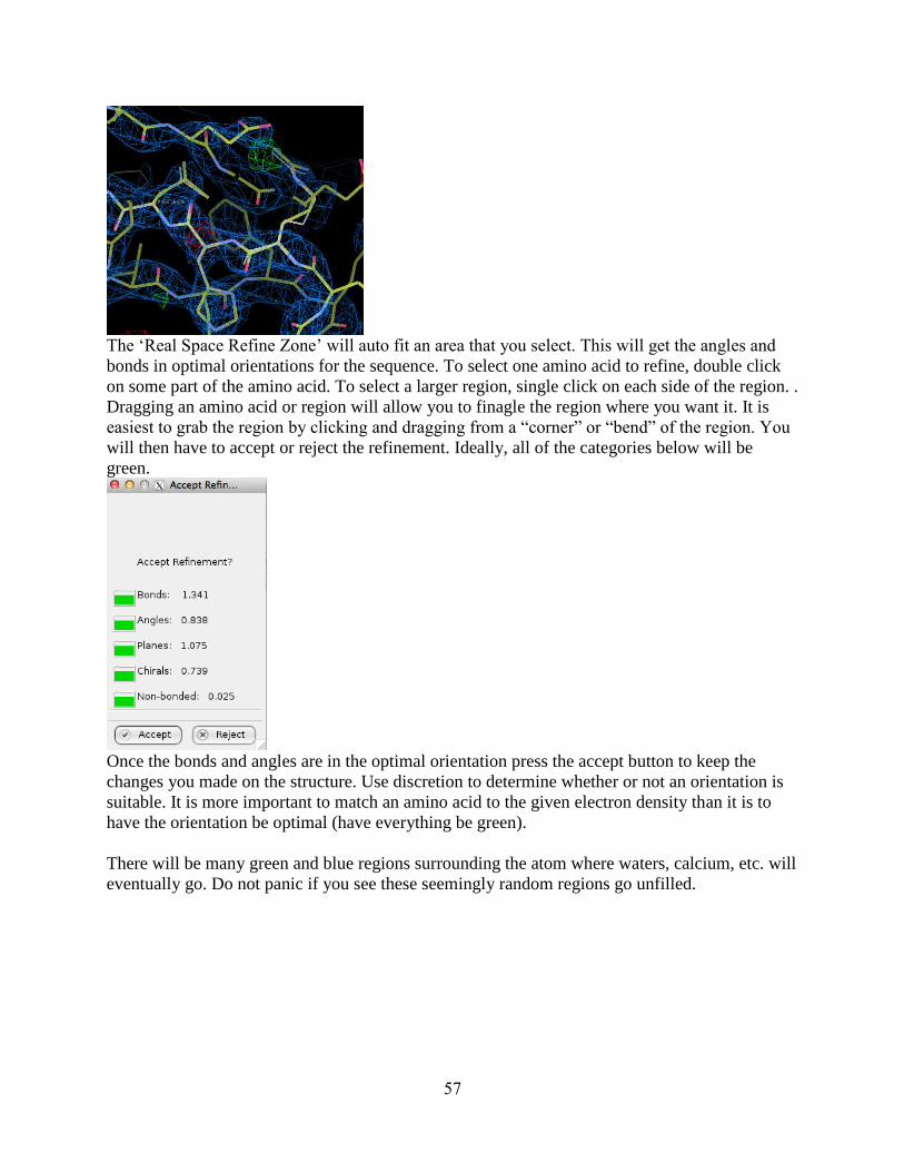
57

The ‘Real Space Refine Zone’ will auto fit an area that you select. This will get the angles and

bonds in optimal orientations for the sequence. To select one amino acid to refine, double click

on some part of the amino acid. To select a larger region, single click on each side of the region. .

Dragging an amino acid or region will allow you to finagle the region where you want it. It is

easiest to grab the region by clicking and dragging from a “corner” or “bend” of the region. You

will then have to accept or reject the refinement. Ideally, all of the categories below will be

green.

Once the bonds and angles are in the optimal orientation press the accept button to keep the

changes you made on the structure. Use discretion to determine whether or not an orientation is

suitable. It is more important to match an amino acid to the given electron density than it is to

have the orientation be optimal (have everything be green).

There will be many green and blue regions surrounding the atom where waters, calcium, etc. will

eventually go. Do not panic if you see these seemingly random regions go unfilled.

58

‘Regularize Zone’ is similar to ‘Real Space Refine Zone’ but may make more drastic changes. If

you are having a lot of difficulty with a region, this may be good place to go as more of a last

resort and may point you in the right direction.

Step 4: Mutate and Auto Fit

If you want to change an amino acid, use the ‘Mutate & Auto Fit’ button from the side menu that

is shown above then select the amino acid you want to change it to. This can also be done with

the ‘Simple Mutate…’ feature, but this will not fit the amino acid to your electron density.

Step 5: Add Terminal Residue

If there is an amino acid missing from the sequence you can add in an amino acid by using the

‘Add Terminal Residue’ button. After clicking it, click on the terminal carbon of your structure

and then on ‘Accept’ in the window that pops up. Make sure that the added amino acid (it will be

faded grey) is inside the electron density on your screen (you can move it by clicking on the grey

amino acid and dragging it) before hitting ‘Accept.’

If the amino acid appears and is not connected to the rest of your chain, simply click ‘Real Space

Refine Zone’ and select an area containing the terminal residue and the newly added amino acid.

The amino acid should then connect.

Step 6: Ramachandran Plots

59

To view the Ramachandran Plot, go to Validate, then Ramachandran Plot, then click on the .pdb

file that you would like to view in the Ramachandran plot. You need to check the Ramachandran

plot before you run the comprehensive validation because to have a good structure meaning that

all the amino acids are in the pink regions on the Ramachandran plot.

As shown in the Ramachandran plot, all the residues need to be in the pink regions (ideally). If

they are not you need to move the residue into the pink region, or at least the yellow region.

When hovering your mouse over a square or triangle, it will show which amino acid that shape

relates to. Those amino acids with squares have different Ramachandran favored regions than

those with triangles.

For a structure to be considered good, you need to have zero “Ramachandran outliers” and

minimal “in allowed regions” (maximum in “favored” regions). Once you have checked this plot

than you can go forward with validating your structure.

A red shape means that the amino acid is a Ramachandran outlier, and should be fixed. A blue

shape means that the amino acid is not an outlier, although it may or may not be in the favored

region. A green shape represents the amino acid you currently have your screen’s focus on. Note

that fixing an amino acid may involve moving the amino acids immediately before and after it.

To fix or move an amino acid’s configuration, you can use the ‘Real Space Refine Zone,’

‘Regularize Zone,’ or ‘Edit Backbone Torsions.’ All of these can be found on the right side of

the Coot window, and ‘Edit Backbone Torsions’ may be the most helpful.

Step 7: Edit Backbone Torsions

Once in the ‘Edit Backbone Torsions’ window, you can either rotate from the peptide or the

carbonyl. Note that this will change the Ramachandran plot for both the amino acid you are

rotating and the one(s) around it. Try to get both shapes in the desired pink region, but make sure

that they stay within the electron density.

60

Step…: Check/Delete Waters

When you have refined a structure using the ‘Update Waters’ feature in the refinement settings,

the program will place waters in spots they do not actually belong. One way to check whether or

not these are likely water spaces, click on ‘Validate,’ then on ‘Check/Delete Waters’ and ‘OK.’

This will bring up a small window in which questionable waters are displayed. Check to see if

the waters in these spots are too close or have too small of an electron density to constitute true

waters. Note that there may be more incorrect waters than those in the questionable water

window and that not all of the questionable waters may be incorrect. Use your best abilities to

discern whether or not there should be waters in each place.

Back to Phenix: Generating Table 1

Step 0: Opening Table 1

On the Phenix home page, navigate to the project you for which you wish to generate a Table 1.

This will give you many values of your structure, including the Rfree, Rwork, correlation

coefficient, resolution, and percent completeness. Under the ‘Utilities’ tab on the Phenix

homepage, click ‘Generate “Table 1” for journal.’ Under the ‘Options’ tab that pop up, make

sure that ‘CSV’ is checked. A .csv file is compatible with Excel and will allow you to view it

there. In the ‘Structure data’ tab, designate the .pdb file, .mtz file, and unmerged data.

Step 1: Unmerge Data

To get an unmerged file of your data, you will need to run HKL2000 again on that project. Run

HKL2000 normally as you did before. Then, after you have scaled your sets (you may want to

put these output files into a different folder or name them something different to tell the

difference between your previous ones), go to the ‘Macros’ tab and input the follow macro to

both the ‘During Integration’ and ‘During Scaling’ lines: no merge original index You will

have to click ‘Add Macro’ when done.

Then, delete the rejection file and re-scale your sets. You will get a message that says something

along the lines of ‘unable to read file… may be because of no merge.’ This is fine since you did

ask HKL to not merge.

Step 2: Using Multiple Data Sets

61

If you had more than one data set for this project, you will again have to run HKL twice and get

two unmerged output files. Like before, you will merge them using CCP4.

Open CCP4 and open ‘Symmetry, Scale, Merge (Aimless).’ Then, in the Aimless window, make

sure that ‘Option to skip scaling and just merge,’ ‘Customize output options,’ ‘Assign to the

same dataset as the previous file,’ and ‘Cell Dimensions’ are checked. Change ‘Input reflection

file type’ to ‘Scalepack file.’ Change ‘MTZ Output’ to ‘scaled, unmerged & no outliers’ and

change ‘Scalepack Output’ to ‘No output.’ You should have SCA #1 and SCA #2 available for

input. Choose your files, set your cell dimensions, and click ‘Run’ and ‘Run Now.’

This will be the ‘Unmerged data’ file in Phenix for generating the Table 1.

Step 3: .pdb and .mtz for Table 1

Your .pdb file will be that of your best refinement. The .mtz file will be the data.mtz file that you

used to refine your .pdb file against. If you can’t remember which ones these were, you can view

it by doing the following. Under the ‘Job history’ tab of Phenix home, double click your best

refinement. Under ‘Configure,’ you can see the files that Phenix used to refine.

62

Appendix C: Tutorial on How to Make Publication Quality Images in PyMOL

Command Description

Color grey50, map Colors the electron density map grey

Set mesh_width, 0.5 Sets the width of the electron density map

mesh

Bg_color white Sets the background color to white

Set ray_trace_fog, 0 Turns off fog

Set depth_cue, 0 Turns off depth cues

Ray Produces a rayed image

Ray 1024, 1024 Produces a rayed image of size 1024x1024

63

References

Ackermann, MA; Shriver, M; Perry, NA; Hu, LR; Kontrogianni-Konstantopoulos, A (2014).

Obscurins: Goliaths and Davids Take Over Non-muscle Tissues. PLoS ONE, 9(2), 1-18.

Afonine, PV; Grosse-Kunstleve, RW; Echols, N; Headd, JJ; Moriarty, NW; Mustyakimov, M;

Terwilliger, TC; Urzhumtsev, A; Zwart, PH; Adams PD (2012). Towards Automated

Crystallographic Structure Refinement with Phenix.Refine. Acta Crystallogr. D Biol.

Crystallogr., 68(Pt 4), 352-367.

Arimura, T; Matsumoto, Y; Okazaki, O; Hayashi, T; Takahashi, M; Inagaki, N; Hinohara, K;

Ashizawa, N; Yano, K; Kimura, A (2007). Structural Analysis of Obscurin Gene in Hypertrophic

Cardiomyopathy. Biochem. Biophys. Res. Commun., 362(2), 281-287.

Armani, A; Galli, S; Giacomello, E; Bagnato, P; Barone, V; Rossi, D; Sorrentino, V (2006).

Molecular Interactions with Obscurin are involved in the Localization of Muscle-specific Small

Ankyrin1 Isoforms to Subcompartments of the Sarcoplasmic Reticulum. Exp. Cell. Res.,

312(18), 3458-3465.

Bang, ML; Centner, T; Fornoff, F; Geach, AJ; Gotthardt, M; McNabb, M; Witt, CC; Labeit, D;

Gregorio, CC; Granzier, H; Labeit, S (2001). The Complete Gene Sequence of Titin, Expression

of an Unusual Approximately 700-kDa Titin Isoform, and its Interaction with Obscurin Identify

a Novel Z-line to I-band Linking System. Circ. Res., 89(11), 1065-1072.

Case, DA; Darden, TA; Cheatham, TE, 3rd; Simmerling, CL; Wang, J; Duke, RE; Luo, R;

Walker, RC; Zhang, W; Merz, KM; Roberts, B; Hayik, S; Roitberg, A; Seabra, G; Swails, J;

Goetz, AW; Kolossváry, I; Wong, KF; Paesani, F; Vanicek, J; Wolf, RM; Liu, J; Wu, X; Brozell,

SR; Steinbrecher, T; Gohlke, H; Cai, Q; Ye, X; Wang, J; Hsieh, M-J; Cui, G; Roe, DR;

Mathews, DH; Seetin, MG; Salomon-Ferrer, R; Sagui, C; Babin, V; Luchko, T; Gusarov, S;

Kovalenko, A; Kollman, PA (2012). AMBER 12. In: University of Califonia SF, Ed. University

of Califonia, San Fransisco.

Chauveau, C; Rowell, J; Ferreiro, A (2014). A Rising Titan: TTN Review and Mutation Update.

Hum. Mutat., 35(9)1046-1059.

Chen, VB; Arendall, WB, 3rd; Headd, JJ; Keedy, DA; Immormino, RM; Kapral, GJ; Murray,

LW; Richardson, JS; Richardson, DC (2010). MolProbity: All-atom Structure Validation for

Macromolecular Crystallography. Acta Crystallogr. D Biol. Crystallogr., 66(1), 12-21.

Chothia, C and Lesk, AM (1986). The Relation between the Diverge of Sequence and Structure

in Proteins. EMBO J., 5(40), 823-826.

Chu, M; Gregorio, CG; and Pappas, CT (2016). Nebulin, a Multi-functional Giant. J. Exp. Biol.,

219, 146-152.

Cooper, GM (2000). The Cell: A Molecular Approach. 2nd Edition, Actin, Myosin, and Cell

Movement. Sinauer Associates, Sunderland, MA.

64

de Groot, BL; van Aalten, DMF; Scheek, RM; Amadei, A; Vriend, G; Berendsen, HJC (1997).

Prediction of Protein Conformational Freedom from Distance Constraints. Proteins 29, 240-251.

Dessau, MA and Modis, Y (2011). Protein Crystallization for X-ray Crystallography. JoVE, 47,

1-6.

Di Cola, E; Waigh, TA; Trinick, J; Tskhovrebova, L; Houmeida, A; Pyckhout-Hintzen, W;

Dewhurst, C (2005). Persistence Length of Titin from Rabbit Skeletal Muscles Measured with

Scattering and Microrheology Techniques. Biophys. J., 88(6), 4095-4106.

Duff, RM; Tay, V; Hackman, P; Ravenscroft, G; McLean, C; Kennedy, P; Steinbach, A;

Schöffler, W; van der Ven, PF; Fürst, DO; Song, J; Djinović-Carugo, K; Penttilä, S; Raheem, O;

Reardon, K; Malandrini, A; Gambelli, S; Villanova, M; Nowak, KJ; Williams, DR; Landers, JE;

Brown, RH, Jr; Udd, B; Laing, NG (2011). Mutations in the N-terminal Actin-binding Domain

of Filamin C Cause a Distal Myopathy. Am. J. Hum. Genet., 88(6), 729-740.

Elliot, P and McKenna, WJ (2004). Hypertrophic Cardiomyopathy. Lancet., 363(9424), 1881-

1891.

Emsley, P; Lohkamp, B; Scott, WG; Cowtan, K (2010). Features and Development of Coot. Acta

Crystallogr. D Biol. Crystallogr., 66(Pt 4), 486-501.

Evilä, A; Vihola, A; Sarparanta, J; Raheem, O; Palmio, J; Sandell, S; Eymard, B; Illa, I; Rojas-

Garcia, R; Hankiewicz, K; Negrão, L, Löppönen, T; Nokelainen, P; Kärppä, M; Penttilä, S;

Screen, M; Suominen, T; Richard, I; Hackman, P; Udd, B (2014). Atypical Phenotypes in

Titinopathies Explained by Second Titin Mutations. Ann. Neurol., 75(2), 230-240.

Freiburg, A; Trombitas, K; Hell, W; Cazorla, O; Fougerousse, F; Centner, T; Kolmerer, B; Witt,

C; Beckmann, JS; Gregorio, CC; Granzier, H; Labeit, S (2000). Series of Exon-skipping Events

in the Elastic Spring Region of Titin as the Structural Basis for Myofibrillar Elastic Diversity.

Circ. Res., 86(11), 1114-1121.

Frenneaux, MP (2004). Assessing the Risk of Sudden Cardiac Death in a Patient with

Hypertrophic Cardiomyopathy. Heart, 90, 570-575.

Fukuzawa, A; Idowu, S; Gautel, M (2005). Complete Human Gene Structure of Obscurin:

Implications for Isoform Generation by Differential Splicing. J. Muscle Res. Cell Motil., 26,

427–434.

Fukuzawa, A; Lange, S; Holt, M; Vihola, A; Carmignac, V; Ferreiro, A; Udd, B; Gautel, M

(2008). Interactions with Titin and Myomesin Target Obscurin and Obscurin-like 1 to the M-

band: Implications for Hereditary Myopathies. J. Cell. Sci., 121(11), 1841-1851.

Garcia, TI; Oberhauser, AF; Braun, W (2009). Mechanical Stability and Differentially

Conserved Physical-chemical Properties of Titin Ig-domains. Proteins 75(3), 706-718.

65

Gautel, M (2011). The Sarcomeric Cytoskeleton: Who Picks Up the Strain? Curr. Opin. Cell

Biol., 23(1), 39-46.

Gautel, M; Djinović-Carugo, K (2016). The Sarcomeric Cytoskeleton: From Molecules to

Motion. J. Exp. Biol., 219(Pt 2), 135-145.

Gold, MG; Barford, D; Komander, D (2006). Lining the Pockets of Kinases and Phosphatases.

Curr. Opin. Struct. Biol., 16, 693-701.

Granzier, HL; Labeit, S (2004). The Giant Protein Titin: A Major Player in Myocardial

Mechanics, Signaling, and Disease. Circ. Res., 94(3), 284-295.

Granzier, HLM; Wang, K (1993). Passive Tension and Stiffness of Vertebrate Skeletal and

Insect Flight Muscles: Contribution of Weak Cross-bridges and Elastic Filaments. Biophys. J.,

65, 2141-2159.

Grater, F; Shen, J; Jiang, H; Gautel, M; Grubmuller, H (2005). Mechanically Induced Titin

Kinase Activation Studied by the Force-probe Molecular Dynamics Simulations. Biophys. J., 88,

790-804.

Greene, DN; Garcia, T; Sutton, RB; Gernert, KM; Benian, GM (2008). Single-molecule Force

Spectroscopy Reveals a Stepwise Unfolding of Caenorhabiditis elegans Giant Protein Kinase

Domains. Biophys. J., 95, 1360-1370.

Guergueltcheva, V; Peeters, K; Baets, J; Ceuterick-de Groote, C; Martin, JJ; Suls, A; De Vriendt,

E; Mihaylova, V; Chamova, T; Almeida-Souza, L; Ydens, E; Tzekov, C; Hadjidekov, G;

Gospodinova, M; Storm, K; Reyniers, E; Bichev, S; van der Ven, PF; Fürst, DO; Mitev, V;

Lochmüller, H; Timmerman, V; Tournev, I; De Jonghe, P; Jordanova, A (2011). Distal

Myopathy with Upper Limb Predominance Caused by Filamin C Haploinsufficiency. Neurology,

77(24), 2105-2114.

Hackman, JP; Vihola, A; Haravuori, H; Marchand, S; Sarparanta, J; De Seze, J; Labiet, S; Witt,

C; Peltonen, L; Richard, I; Udd, B (2002). Tibial Muscular Dystrophy is a Titinopathy Caused

by Mutations in TTN, the Gene Encoding the Giant Skeletal-Muscle Protein Titin. Am. J. Hum.

Genet., 71, 492-500.

Hornak, V; Abel, R; Okur, A; Strockbine, B; Roitberg, A; Simmerling, C (2006). Comparison of

multiple Amber force fields and development of improved protein backbone parameters.

Proteins, 65, 712-725.

Hsin, J; Strumpfer, J; Lee, EH; Schulten, K (2011). Molecular Origin of the Hierarchical

Elasticity of Titin: Simulation, Experiment, and Theory. Annu. Rev. Biophys., 40, 187-203.

Hu, LR and Kontrogianni-Konstantopoulos, A (2013). The Kinase Domains of Obscurin Interact

with Intercellular Adhesion Proteins. FASEB J., 27(5), 2001-2012.

66

Hu, SH; Parker, MW; Lei, JY; Wilce, MC; Benian, GM; Kemp, BE (1994). Insights into

Autoregulation from the Crystal Structure of Twitchin Kinase. Nature, 369, 581-584.

Hu, YR; Ackermann, M; Hecker, P; Prosser, B; King, B; O’Connell, K; Asico, L; Jose, P;

Wright, N; Lederer, J; Kontrogianni-Konstantopulous, A (2016). A Missense Mutation in the

Obscurin Gene Leads to Hypertrophic Cardiomyopathy due to Deregulated Calcium Cycling.

Biophys. J., 110, 618a.

Improta, S; Krueger, JK; Gautel, M; Atkinson, RA; Lefevre, JF; Moulton, S; Trewhella, J;

Pastore, A (1998). The Assembly of Immunoglobulin-like Modules in Titin: Implications for

Muscle Elasticity. J. Mol. Biol., 284, 761-777.

Isralewitz, B; Gao, M; Schulten, K (2001). Steered Molecular Dynamics and Mechanical

Functions of Proteins. Curr. Opin. Struct. Biol., 11(2), 224-230.

Johnson, DA; Akamine, P; Radzio-Andzelm, E; Madhusudan, M; Taylor, SS (2001). Dynamics

of cAMP-dependent Protein Kinase. Chem. Rev., 101, 2243-2270.

Kley, RA; Serdaroglu-Oflazer, P; Leber, Y; Odgerel, Z; van der Ven, PF; Olivé, M; Ferrer, I;

Onipe, A; Mihaylov, M; Bilbao, JM; Lee, HS; Höhfeld, J; Djinović-Carugo, K; Kong, K;

Tegenthoff, M; Peters, SA; Stenzel, W; Vorgerd, M; Goldfarb, LG; Fürst, DO (2012).

Pathophysiology of Protein Aggregation and Extended Phenotyping in Filaminopathy. Brain,

135(Pt 9), 2642-2660.

Kobe, B; Heierhorst, J; Feil, SC; Parker, MW; Benian, GM; Weiss, KR; Kemp, BE (1996). Giant

Protein Kinases: Domain Interactions and Structural Basis of Autoregulation. EMBO J., 15,

6810-6821.

Kontrogianni-Konstantopoulos, A and Bloch, RJ (2005). Obscurin: A Multitasking Muscle

Giant. J. Muscle Res. Cell Motil., 26(6-8), 419-426.

Kontrogianni-Konstantopoulos, A; Ackermann, MA; Bowmann, AL; Yap, SV; and Bloch, RJ

(2009). Muscle Giants: Molecular Scaffolds in Sarcomerogenesis. Physiol. Rev., 89(4), 1217-

1267.

Kopot, A (2014). Contraction of Skeletal Muscle. AK Lectures.

Krieger, E; Darden, T; Nabuurs, SB; Finkelstein, A; Vriend, G (2004). Making Optimal Use of

Empirical Energy Functions: Force-field Parameterization in Crystal Space. Proteins, 57(4),

678−683.

Krieger, E; Vriend, G (2014). YASARA View - Molecular Graphics for All Devices - from

Smartphones to Workstations. Bioinformatics, 30(20), 2981-2982.

Lee, EH; Hsin, J; Mayans, O; Schulten, K (2007). Secondary and Tertiary Structure Elasticity of

Titin Z1Z2 and a Titin Chain Model. Biophys. J., 93(5), 1719-1735.

67

Lee, W; Tonelli, M; Markley, JL (2015). NMRFAM-SPARKY: Enhanced Software for

Biomolecular NMR Spectroscopy. Bioinformatics, 31, 1325-1327.

Li, H and Fernandez, JM (2003). Mechanical Design of the First Proximal Ig Domain of Human

Cardiac Titin Revealed by Single Molecule Force Spectroscopy. J. Mol. Biol., 334(1), 75-86.

Li, H; Linke, WA; Oberhauser, AF; Carrion-Vazquez, M; Kerkvliet, JG; Lu, H; Marszalek, PE;

Fernandez, JM (2002). Reverse Engineering of the Giant Muscle Protein Titin. Nature, 418, 998-

1002.

Linke, WA (2000). Stretching Molecular Springs: Elasticity of Titin Filaments in Vertebrate

Striated Muscle. Histol. Histopathol., 15(3), 799-811.

Linke, WA (2000). Titin Elasticity in the Context of the Sarcomere: Force and Extensibility

Measurements on Single Myofibrils. Avd. Exp. Med. Biol., 481, 179-202; discussion 203-176.

Linke, WA (2008). Sense and Stretchability: The Role of Titin and Titin-associated Proteins in

Myocardial Stress-sensing and Mechanical Dysfunction. Cardiovasc. Res., 77, 637-648.

Linke, WA; Popov, VI; Pollack, GH (1994). Passive and Active Tension in Single Cardiac

Myofibrils. Biophys. J., 67, 782-792.

Löwe, T; Kley, RA; van der Ven, PF; Himmel, M; Huebner, A; Vorgerd, M; Fürst, DO (2007).

The Pathomechanism of Filaminopathy: Altered Biochemical Properties Explain the Cellular

Phenotype of a Protein Aggregation Myopathy. Hum. Mol. Genet., 16(11), 1351-1358.

Luan, X; Hong, D; Zhang, W; Wang, Z; Yuan, Y (2010). A Novel Heterozygous Deletion-

insertion Mutation (2695-2712 del/GTTTGT ins) in Exon 18 of the Filamin C Gene Causes

Filaminopathy in a Large Chinese Family. Neuromuscul. Disord., 20(6), 390-396.

Ma, K; Kan, L; Wang, K (2001). Polyproline II Helix is a Key Structural Motif of the Elastic

PEVK Segment of Titin. Biochemistry, 40(12), 3427-3438.

Ma, K; Wang, K (2003). Malleable Conformation of the Elastic PEVK Segment of Titin: Non-

co-operative Interconversion of Polyproline II Helix, Beta-turn and Unordered Structures.

Biochem. J., 374(Pt 3), 687-695.

Marchetti, S; Sbrana, F; Toscano, A; Fratini, E; Carla, M; Vassalli, M; Tiribilli, B; Pacini, A;

Gambi, CM (2011). Beta-connectin Studies by Small-angle X-ray Scattering and Single-

molecule Force Spectroscopy by Atomic Force Microscopy. Phys. Rev. E Stat. Nonlin. Soft

Matter Phys., 83(5 Pt 1), 051919.

Marino, M; Zou, P; Svergun, D; Garcia, P; Edlich, C; Simon, B; Wilmanns, M; Muhle-Goll, C;

Mayans, O (2006). The Ig Doublet Z1Z2: a Model System for the Hybrid Analysis of

Conformational Dynamics in Ig Tandems from Titin. Structure, 14(9), 1437-1447.

68

Marston, S; Montgiraud, C; Munster, AB; Copeland, O; Choi, O; Dos Remedios, C; Messer, AE;

Ehler, E; Knöll, R (2015). OBSCN Mutations Associated with Dilated Cardiomyopathy and

Haploinsufficiency. PLoS One, 10(9), e0138568.

Mastaglia, FL; Laing, NG (1999). Distal Myopathies: Clinical and Molecular Diagnosis and

Classification. J. Neurol. Neurosurg. Psychiatry., 67(6), 703-707.

Mastersona, LR; Masterson, LR; Shi, L; Metcalfe, E; Gao, J; Taylor, SS; Veglia, G (2011).

Dynamically Committed, Uncommitted, and Quenched States Encoded in Protein Kinase A

Revealed by NMR Spectroscopy. Proc. Natl. Acad. Sci. U.S.A., 108, 6969-6974.

Matsubara, S; Maruyama, K (1977). Role of Connectin in the Length-tension Relation of

Skeletal and Cardiac Muscles. Jpn J. Physiol., 27(5), 589-600.

Mayans, O; Benian, GM; Simkovic, F; Rigden, DJ (2012). Mechanistic and Functional Diversity

in the Mechanosensory Kinases of the Titin-like Family. Biochem. Soc. Trans., 41(Pt 4), 1066-

71.

Mayans, O; van der Ven, PFM; Wilm, M; Mues, A; Young, P; Fürst, DO; Wilmanns, M; Gautel,

M (1998). Structural Basis for Activation of the Titin Kinase Domain during Myofibrillogenesis.

Nature, 395, 863-869.

McNally, EM and Pytel, P (2007). Muscle Diseases: the Muscular Dystrophies. Annu. Rev.

Pathol., 2, 87-109.

Meyer, LC and Wright, NT (2003). Structure of Giant Muscle Proteins. Front. Physiol., 4, 368,

1-12.

Muntoni, F; Wells, D (2007). Genetic Treatments in Muscular Dystrophies. Curr. Opin. Neurol.,

20(5), 590-594.

Nagase, T; Kikuno, R; Hattori, A; Kondo, Y; Okumura K, Ohara, O (2000). Prediction of the

Coding Sequences of Unidentified Human Genes. XIX. The Complete Sequences of 100 New

cDNA Clones from Brain which Code for Large Proteins in vitro. DNA Res., 7, 347–355.

Nagase, T; Kikuno, R; Ishikawa, KI; Hirosawa, M; Ohara, O (2000). Prediction of the Coding

Sequences of Unidentified Human Genes. XVI. The Complete Sequences of 150 New cDNA

Clones from Brain which Code for Large Proteins in vitro. DNA Res., 7, 65-73.

Nagase, T; Kikuno, R; Nakayama, M; Hirosawa, M; Ohara, O (2000). Prediction of the Coding

Sequences of Unidentified Human Genes. XVIII. The Complete Sequences of 100 New cDNA

Clones from Brain which Code for Large Proteins in vitro. DNA Res., 7, 273-281.

Ng, R; Banks, GB; Hall, JK; Muir, LA; Ramos, JN; Wicki, J; Odom, GL; Konieczny, P; Seto, J;

Chamberlain, JR; Chamberlain, JS (2012). Animal Models of Muscular dystrophy. Prog. Mol.

Biol. Transl. Sci., 105, 83-111.

69

Nguyen, H; Roe, DR; Simmerling, C (2013). Improved Generalized Born Solvent Model

Parameters for Protein Simulations. J. Chem. Theory Comput., 9(4), 2020-2034.

Otwinowski, Z; Minor, W (1997). Processing of X-ray Diffraction Data Collected in Oscillation

Mode. Methods Enzymol., 276, 307-326.

Pernigo, S; Fukuzawa, A; Bertz, M; Holt, M; Rief, M; Steiner, RA; Gautel, M (2010). Structural

Insight into M-band Assembly and Mechanics from the Titin-obscurin-like-1 complex. Proc.

Natl. Acad. Sci. USA, 107(7), 2908-2913.

Perry, NA; Vitolo, MI; Martin, SS; Kontrogianni-Konstantopoulos, A (2014). Loss of Obscurin-

RhoGEF Downregulates RhoA Signaling and Increases Microtentacle Formation and

Attachment of Breast Epithelial Cells. Oncotarget, 5(18), 8558-8568.

Puchner, EM and Gaub, HE (2010). Exploring the Conformation-regulated Function of Titin

Kinase by Mechanical Pump and Probe Experiments with Single Molecules. Angew. Chem. Int.

Ed., 49, 1147-1150.

Puchner, EM; Alexandrovich, A; Kho, AL; Hensen, U; Schafer, LV; Brandmeier, B; Grater, F;

Grubmuller, H; Gaub, HE; Gautel, M (2008). Mechanoenzymatics of Titin Kinase. Proc. Natl.,

Acad. Sci. U.S.A., 105, 13385-13390.

Randazzo, D; Blaauw, B; Paolini, C; Pierantozzi, E; Spinozzi, S; Lange, S; Chen, J; Protasi, F;

Reggiani, C; Sorrentino, V (2017). Exercise-induced Alterations and Loss of Sarcomeric M-line

Organization in the Diaphragm Muscle of Obscurin Knockout Mice. Am. J. Physiol. Cell.

Physiol., 312(1), C16-C28.

Randazzo, D; Giacomello, E; Lorenzini, S; Rossi, D; Pierantozzi, E; Blaauw, B; Reggiani, C;

Lange, S; Peter, AK; Chen, J; Sorrentino, V (2013). Obscurin is Required for AnkyrinB-

dependent Dystrophin Localization and Sarcolemma Integrity. J. Cell. Biol., 200(4), 523-536.

Razinia, Z; Mäkelä, T; Ylänne, J; Calderwood, DA (2012). Filamins in Mechanosensing and

Signaling. Annu. Rev. Biophys., 41, 227-46.

Rhodes, G (2006). Crystallography Made Crystal Clear, Third Edition. Elsevier Inc., Burlington,

MA.

Rief, M; Gautel, M; Gaub, HE (2000). Unfolding Forces of Titin and Fibronectin Domains

Directly Measured by AFM. Adv. Exp. Med. Biol., 481:129-136; discussion 137-141.

Rossi, D; Bencini, C; Maritati, M; Benini, F; Lorenzini, S; Pierantozzi, E; Scarcella, AM;

Paolini, C; Protasi, F; Sorrentino, V (2014). Distinct Regions of Triadin are Required for

Targeting and Retention at the Junctional Domain of the Sarcoplasmic Reticulum. Biochem. J.,

458(2), 407-417.

70

Rossi, D; Palmio, J; Evila, A; Galli, L; Barone, V; Caldwell, TA; Policke, RA; Berndsen, CE;

Wright, NT; Romero, N; Malfatti, E; Brochier, G; Stokkovic, T; Jordanova, A; Guergueltcheva,

A; Hackman, P; Romero, NB; Eymard, B; Udd, B; Sorrentino, V (submitted). Digenic

Inheritance of a FLNC Frameshift and an OBSCN Variant in a Family with Distal Muscular

Dystrophy.

Rossi, D; Vezzani, B; Galli, L; Paolini, C; Toniolo, L; Pierantozzi, E; Spinozzi, S; Barone, V;

Pegoraro, E; Bello, L; Cenacchi, G; Vattemi, G; Tomelleri, G; Ricci, G; Siciliano, G; Protasi, F;

Reggiani, C; Sorrentino, V (2014). A Mutation in the CASQ1 Gene Causes a Vacuolar

Myopathy with Accumulation of Sarcoplasmic Reticulum Protein Aggregates. Hum. Mutat.,

35(10), 1163-1170.

Rudloff, MW; Woosley, AN; Wright, NT (2015). Biophysical Characterization of Naturally

Occurring Titin M10 Mutations. Protein Sci., 24(6), 946-955.

Rupp, B (2010). Biomolecular Crytallography. Garland Science, Taylor and Francis Group, New

York, New York.

Russell, MW; Raeker, MO; Korytkowski, KA; Sonneman, KJ (2002). Identification, Tissue

Expression and Chromosomal Localization of Obscurin-MLCK, a Member of the Titin and Dbl

Families of Myosin Light Chain Kinases. Gene., 282, 237-246.

Satoh, M; Takahashi, M; Sakamoto, T; Hiroe, M; Marumo, F; Kimura, A (1999). Structural

Analysis of the Titin Gene in Hypertrophic Cardiomyopathy: Identification of a Novel Disease

Gene. Biochem. Biophys. Res. Commun., 262, 411-417.

Scapin, G (2013). Molecular Replacement Then and Now. Acta. Crystallogr. D. Biol.

Crystallogr., 69(11), 2266-2275.

Sewry, CA (2010). Muscular Dystrophies: An Update on Pathology and Diagnosis. Acta

Neuropathol., 120(3), 343-358.

Shatunov, A; Olivé, M; Odgerel, Z; Stadelmann-Nessler, C; Irlbacher, K; van Landeghem, F;

Bayarsaikhan, M; Lee, HS; Goudeau, B; Chinnery, PF; Straub, V; Hilton-Jones, D; Damian, MS;

Kaminska, A; Vicart, P; Bushby, K; Dalakas, MC; Sambuughin, N; Ferrer, I; Goebel, HH;

Goldfarb, LG (2009). In-frame Deletion in the Seventh Immunoglobulin-like Repeat of Filamin

C in a Family with Myofibrillar Myopathy. Eur. J. Hum. Genet., 17(5), 656-663.

Shen, Y; Delaglio, F; Cornilescu, G; Bax, A (2009). TALOS+: A Hybrid Method for Predicting

Protein Backbone Torsion Angles from NMR Chemical Shifts J. Biomol. NMR, 44(4), 213-223.

Shriver, M; Marimuthu, S; Paul, C; Geist, J; Seale, T; Konstantopoulos, K; Kontrogianni-

Konstantopoulos, A (2016). Giant Obscurins Regulate the PI3K Cascade in Breast Epithelial

Cells via Direct Binding to the PI3K/p85 Regulatory Subunit. Oncotarget, 7(29), 45414-45428.

71

Sjoblom, T.; Jones, S.; Wood, L. D.; Parsons, D. W.; Lin, J.; Barber, T. D.; Mandelker, D.;

Leary, R. J.; Ptak, J.; Silliman, N.; Szabo, S.; Buckhaults, P.; Farrell, C.; Meeh, P.; Markowitz,

S. D.; Willis, J.; Dawson, D.; Willson, J. K.; Gazdar, A. F.; Hartigan, J.; Wu, L.; Liu, C.;

Parmigiani, G.; Park, B. H.; Bachman, K. E.; Papadopoulos, N.; Vogelstein, B.; Kinzler, K. W.;

Velculescu, V. E (2006). The Consensus Coding Sequences of Human Breast and Colorectal

Cancers. Science, 314 (5797), 268-74.

Stacklies, W; Vega, MC; Wilmanns, M; Grater, F (2009). Mechanical Network in Titin

Immunoglobulin from Force Distribution Analysis. PLoS Comput. Biol., 5(3), e1000306.

Stahl, SW; Puchner, EM; Alexandrovich, A; Gautel, M; Gaub, HE (2011). A Conditional Gating

Mechanism Assures the Integrity of the Molecular Force-sensor Titin Kinase. Biophys. J., 101,

1978-1986.

Stroka, KM; Wong, BS; Shriver, M; Phillip, JM; Wirtz, D; Kontrogianni-Konstantopoulos, A;

Konstantopoulos, K (2016). Loss of Giant Obscurins Alters Breast Epithelian Cell

Mechanosensing of Matrix Stiffness. Oncotarget, Advanced Publications, 1-17.

Tsai, CJ; Nussinov, R (2013). The Molecular Basis of Targeting Protein Kinases in Cancer

Therapeutics. Semin. Cancer Biol., 23(4), 235-242.

Teekakirikul, P; Padera, RF; Seidman, JG; Seidman, CE (2012). Hypertrophic Cardiomyopathy:

Translating Cellular Cross Talk into Therapeutics. J. Cell. Biol., 199(3), 417-421.

Terwilliger, TC; Grosse-Kunstleve, RW; Afonine, PV; Moriarty, NW; Zwart, PH; Hung, LW;

Read, RJ; Adams, PD (2008). Iterative Model Building, Structure Refinement and Density

Modification with the PHENIX AutoBuild Wizard. Acta Crystallogr. D Biol. Crystallogr., 64(1),

61-69.

The PyMOL Molecular Graphics System, Version 1.3 Schrödinger, LLC.

Trinick, J (1992). Understanding the Functions of Titin and Nebulin. FEBS Lett., 307(1), 44-48.

Udd, B (2012). Distal Myopathies- New Genetic Entities Expand Diagnostic Challenge.

Neuromuscul. Disord., 22(1), 5-12.

Udd, B; Griggs, R (2001). Distal Myopathies. Curr. Opin. Neurol., 14, 561-566.

van Zundert, GCP; Rodrigues, JPGLM; Trellet, M; Schmitz, C; Kastritis, PL; Karaca, E;

Melquiond, ASJ; de Vries, SJ; Bonvin, AMJJ (2016). The HADDOCK2.2 Web Server: User-

friendly Integrative Modeling of Biomolecular Complexes. J. Mol. Biol., 428(4), 720-725.

Vazina, AA; Lanina, NF; Alexeev, DG; Bras, W; Dolbnya, IP (2006). The Structural Principles

of Multidomain Organization of the Giant Polypeptide Chain of the Muscle Titin Protein:

SAXS/WAXS Studies during the Stretching of Oriented Titin Fibres. J. Struct. Biol., 155(2),

251-262.

72

von Castelmur, E; Marino, M; Svergun, DI; Kreplak, L; Ucurum-Fotiadis, Z; Konarev, PV;

Urzhumtsev, A; Labeit, D; Labeit, S; Mayans, O (2008). A Regular Pattern of Ig Super-motifs

Defines Segmental Flexibility as the Elastic Mechanism of the Titin Chain. Proc. Natl. Acad.

Sci. U.S.A., 105(4), 1186-1191.

Vorgerd, M; van der Ven, PF; Bruchertseifer, V; Löwe, T; Kley, RA; Schröder, R; Lochmüller,

H; Himmel, M; Koehler, K; Fürst, DO; Huebner, A (2005). A Mutation in the Dimerization

Domain of Filamin C Causes a Novel Type of Autosomal Dominant Myofibrillar Myopathy. Am.

J. Hum. Genet., 77(2), 297-304.

Wlodawer, A; Wladek, M; Dauter, Z; Jaskolski, M (2008). Protein Crystallography for Non-

crystallographers, or How to Get the Best (but not more) from Published Macromolecular

Structures. FEBS J., 275(1), 1-21.

Wlodawer, A; Wladek, M; Dauter, Z; Jaskolski, M (2013). Protein Crystallography for Aspiring

Crystallographers or How to Avoid Pitfalls and Traps in Macromolecular Structure

Determination. FEBS J., 280(22), 5705-5736.

Wood, L. D.; Parsons, D. W.; Jones, S.; Lin, J.; Sjoblom, T.; Leary, R. J.; Shen, D.; Boca, S. M.;

Barber, T.; Ptak, J.; Silliman, N.; Szabo, S.; Dezso, Z.; Ustyanksky, V.; Nikolskaya, T.;

Nikolsky, Y.; Karchin, R.; Wilson, P. A.; Kaminker, J. S.; Zhang, Z.; Croshaw, R.; Willis, J.;

Dawson, D.; Shipitsin, M.; Willson, J. K.; Sukumar, S.; Polyak, K.; Park, B. H.; Pethiyagoda, C.

L.; Pant, P. V.; Ballinger, D. G.; Sparks, A. B.; Hartigan, J.; Smith, D. R.; Suh, E.;

Papadopoulos, N.; Buckhaults, P.; Markowitz, S. D.; Parmigiani, G.; Kinzler, K. W.; Velculescu,

V. E.; Vogelstein, B (2007). The Genomic Landscapes of Human Breast and Colorectal Cancers.

Science, 318 (5853), 1108-13.

Wright, NT; Varney, KM; Ellis, KC; Markowitz, J; Gitti, RK; Zimmer, DB; Weber, DJ (2005).

The Three-dimensional Solution Structure of Ca(2+)-bound S100A1 as Determined by NMR

Spectroscopy. J. Mol. Biol., 353(2), 410-426.

Yang, J; Roy, A; Zhang, Y (2013). Protein-ligand Binding Site Recognition using

Complementary Binding-specific Substructure Comparison and Sequence Profile Alignment.

Bioinformatics, 29(20), 2588-2595.

Young, P; Ehler, E; Gautel, M (2001). Obscurin, a Giant Sarcomeric Rho Guanine Nucleotide

Exchange Factor Protein Involved in Sarcomere Assembly. J. Cell. Biol., 154, 123-136.

Zheng, W; Chen, H; Deng, X; Yuan, L; Yang, Y; Song, Z; Yang, Z; Wu, Y; Deng, H (2015).

Identification of a Novel Mutation in the Titin Gene in a Chinese Family with Limb-Girdle

Muscular Dystrophy 2J. Mol. Neurobiol., [Epub ahead of print].