studies into the detection of buried objects (particularly...
TRANSCRIPT
Studies into the Detection of Buried Objects (Particularly
Optical Fibres) in Saturated Sediment. Part 5: An Acousto-Optic Detection System
R.C.P. Evans and T.G. Leighton
ISVR Technical Report No 313
April 2007
SCIENTIFIC PUBLICATIONS BY THE ISVR
Technical Reports are published to promote timely dissemination of research results by ISVR personnel. This medium permits more detailed presentation than is usually acceptable for scientific journals. Responsibility for both the content and any opinions expressed rests entirely with the author(s). Technical Memoranda are produced to enable the early or preliminary release of information by ISVR personnel where such release is deemed to the appropriate. Information contained in these memoranda may be incomplete, or form part of a continuing programme; this should be borne in mind when using or quoting from these documents. Contract Reports are produced to record the results of scientific work carried out for sponsors, under contract. The ISVR treats these reports as confidential to sponsors and does not make them available for general circulation. Individual sponsors may, however, authorize subsequent release of the material. COPYRIGHT NOTICE (c) ISVR University of Southampton All rights reserved. ISVR authorises you to view and download the Materials at this Web site ("Site") only for your personal, non-commercial use. This authorization is not a transfer of title in the Materials and copies of the Materials and is subject to the following restrictions: 1) you must retain, on all copies of the Materials downloaded, all copyright and other proprietary notices contained in the Materials; 2) you may not modify the Materials in any way or reproduce or publicly display, perform, or distribute or otherwise use them for any public or commercial purpose; and 3) you must not transfer the Materials to any other person unless you give them notice of, and they agree to accept, the obligations arising under these terms and conditions of use. You agree to abide by all additional restrictions displayed on the Site as it may be updated from time to time. This Site, including all Materials, is protected by worldwide copyright laws and treaty provisions. You agree to comply with all copyright laws worldwide in your use of this Site and to prevent any unauthorised copying of the Materials.
Studies into the detection of buried objects (particularly optical fibres) in saturated sediment. Part 5: An acousto-optic detection system
R C P Evans and T G Leighton
ISVR Technical Report No. 313
April 2007
2
UNIVERSITY OF SOUTHAMPTON
INSTITUTE OF SOUND AND VIBRATION RESEARCH
FLUID DYNAMICS AND ACOUSTICS GROUP
Studies into the detection of buried objects (particularly optical fibres) in saturated sediment. Part 5: An acousto-optic detection system
by
R C P Evans and T G Leighton
ISVR Technical Report No. 313
April 2007
Authorized for issue by Professor R J Astley, Group Chairman
© Institute of Sound & Vibration Research

ii
ACKNOWLEDGEMENTS
TGL is grateful to the Engineering and Physical Sciences Research Council and Cable
& Wireless for providing a studentship for RCPE to conduct this project.

iii
CONTENTS
ACKNOWLEDGEMENTS ii
CONTENTS III
FIGURE CAPTIONS V ABSTRACT viii
1 INTRODUCTION 1
2 DISTRIBUTED FIBRE OPTIC SENSORS 3
2.1 Scattering in Optic Fibres 4
2.2 Back-Scatter Sensors 5
2.3 Optical Time-Domain Reflectometry 6
2.4 Practical Considerations 8
3 NON-LINEARITY IN FIBRE TRANSMISSION 11
3.1 Brillouin Scattering 13
4 BRILLOUIN BACK-SCATTER SYSTEMS 16
4.1 Temperature Dependence of the Brillouin Shift 17
4.2 Strain Dependence of the Brillouin Shift 17
5 OPTIC FIBRE HYDROPHONES 18
6 OTDR EXPERIMENT 22
7 SUMMARY 27
APPENDIX A 30

iv
OPTIC FIBRE PRESSURE SENSITIVITY 30
A.1 CALCULATION OF PRESSURE SENSITIVITY 30
REFERENCES 34
v
FIGURE CAPTIONS
Figure 1 The detection protocol associated with an acousto-optic detection
system. In this scenario, an acoustic beam is projected from a surface vessel
(though it could also be projected from an ROV). As the footprint of the
beam passes over cable B, its affect on the optical transmission properties of
the inner fibres may be detected using a land-based system. By comparing
the position of the footprint over time with the time of detection, it should be
possible to determine the location of the cable.
2
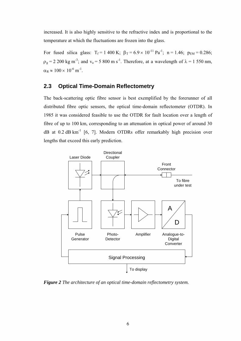
Figure 2 The architecture of an optical time-domain reflectometry system.
6
Figure 3 The OTDR output trace. The intensity of the back-scattered signal
is displayed as a function of time (proportional to fibre length). An almost
constant attenuation is observed over the length of the fibre except at point
X where some external influence has caused the attenuation to increase.
7
Figure 4 The characteristic optical attenuation spectrum of glass optic
fibres [10].
10
Figure 5 The positions of Rayleigh, Brillouin and Raman scattered light
relative to the incident light beam of frequency, f0 [3]. (Note that these axes
are not to scale.)
12
Figure 6 Bragg scattering from periodic refractive index variations in an
otherwise homogeneous medium. The scattered beam will only be coherent
if the path length, ( )2 2λ θr ssin , is an integer multiple of the wavelength of
the incident beam, λ p rn .
14

vi
Table 1 The composition, dimensions and elastic and elasto-optic
coefficients of a typical single mode optic fibre.
20
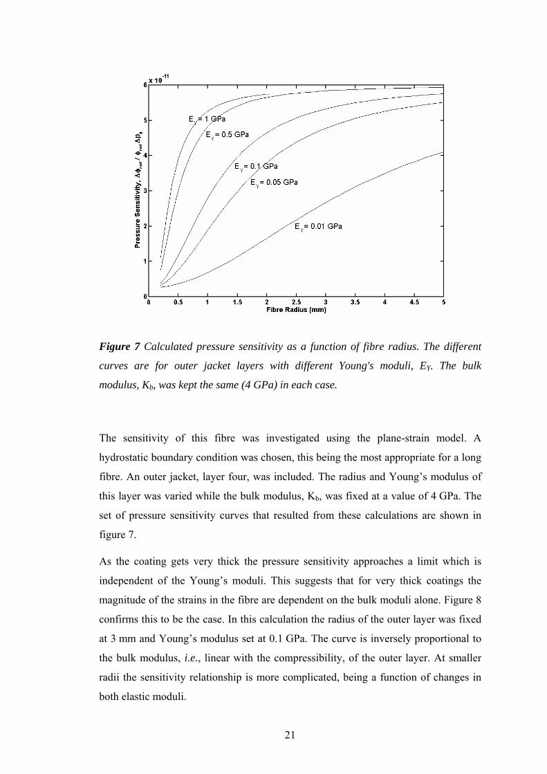
Figure 7 Calculated pressure sensitivity as a function of fibre radius. The
different curves are for outer jacket layers with different Young's moduli, EY.
The bulk modulus, Kb, was kept the same (4 GPa) in each case.
21
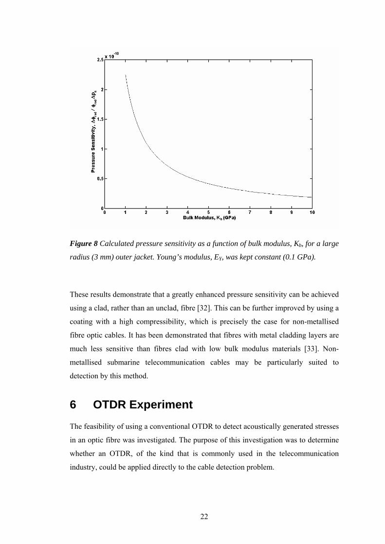
Figure 8 Calculated pressure sensitivity as a function of bulk modulus, Kb,
for a large radius (3 mm) outer jacket. Young’s modulus, EY, was kept
constant (0.1 GPa).
22
Figure 9 The apparatus used in the OTDR experiment. The OTDR was
connected to a 1.8 km length of optic fibre wound on a mandrel. The final
8 m of fibre was wound through a submerged tubular acoustic source. The
fibre was excited using the acoustic source, and the back-scattered optical
signal was measured using the OTDR.
23
Figure 10 An example of the OTDR output trace with no acoustic excitation.
Back-scattered optical power is displayed as a function of distance. The
decrease in the region between the two cursors was caused by radiation at
bends in the fibre. The distinct reflection from the end of the fibre can be
seen one metre beyond this region. (Note that the end-reflection has been
clipped to allow the region between the two cursors to be resolved.)
24
vii
Figure 11 Two sets of data (+, ×) showing back-scattered optical power in
decibels as a function of the acoustic excitation frequency. The values were
calculated relative to the back-scattered optical power in the case when
there was no acoustic excitation. A best-fit curve for the combined data sets
is shown by the solid curve.
25
Figure A 1 The geometry of the multi-layered cylinder representation of a
jacketed optic fibre.
30
viii
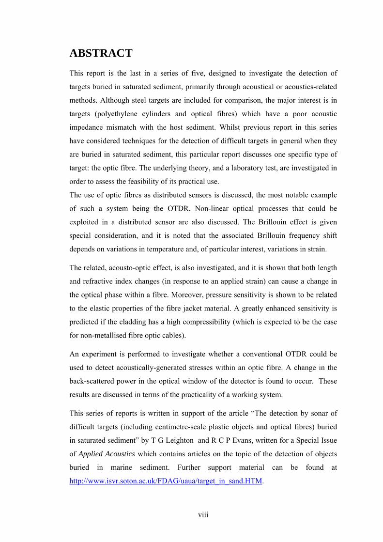
ABSTRACT
This report is the last in a series of five, designed to investigate the detection of
targets buried in saturated sediment, primarily through acoustical or acoustics-related
methods. Although steel targets are included for comparison, the major interest is in
targets (polyethylene cylinders and optical fibres) which have a poor acoustic
impedance mismatch with the host sediment. Whilst previous report in this series
have considered techniques for the detection of difficult targets in general when they
are buried in saturated sediment, this particular report discusses one specific type of
target: the optic fibre. The underlying theory, and a laboratory test, are investigated in
order to assess the feasibility of its practical use.
The use of optic fibres as distributed sensors is discussed, the most notable example
of such a system being the OTDR. Non-linear optical processes that could be
exploited in a distributed sensor are also discussed. The Brillouin effect is given
special consideration, and it is noted that the associated Brillouin frequency shift
depends on variations in temperature and, of particular interest, variations in strain.
The related, acousto-optic effect, is also investigated, and it is shown that both length
and refractive index changes (in response to an applied strain) can cause a change in
the optical phase within a fibre. Moreover, pressure sensitivity is shown to be related
to the elastic properties of the fibre jacket material. A greatly enhanced sensitivity is
predicted if the cladding has a high compressibility (which is expected to be the case
for non-metallised fibre optic cables).
An experiment is performed to investigate whether a conventional OTDR could be
used to detect acoustically-generated stresses within an optic fibre. A change in the
back-scattered power in the optical window of the detector is found to occur. These
results are discussed in terms of the practicality of a working system.
This series of reports is written in support of the article “The detection by sonar of
difficult targets (including centimetre-scale plastic objects and optical fibres) buried
in saturated sediment” by T G Leighton and R C P Evans, written for a Special Issue
of Applied Acoustics which contains articles on the topic of the detection of objects
buried in marine sediment. Further support material can be found at
http://www.isvr.soton.ac.uk/FDAG/uaua/target_in_sand.HTM.
ix
LIST OF SYMBOLS
a An adjustment variable
b An adjustment variable
c An adjustment variable
cg Speed of light in a glass fibre
e Exponential constant (2.71828182)
EY Young’s modulus (i)YE Young’s modulus of a layer in a multilayer cylinder (where the use of (i)
defines the layer of interest in a multilayer cylinder, such that i=0
corresponds to the core)
F Net axial force
f0 Carrier frequency of light beam
fk Acoustic frequency in kilohertz
i An index related to the layers in an optic fibre, where i = 0 denotes the
core, and i = n denotes the nth layer
ka Wave vector of an acoustic wave
Kb Bulk modulus
kB Wave vector of a Brillouin signal
kp Wave vector of an optical pump signal
l Length
LPR Landau-Placzek ratio
m A positive integer variable
n A non-zero positive integer denoting the number of layers in the
x
multilayer cylinder which represents a given optical fibre
NA Numerical aperture
nc Refractive index of the cladding of an optic fibre
nf Refractive index of the core of an optic fibre
nr Refractive index
∆nr Change in refractive index when a material is deformed
p0 Pressure acting on the outer surface of the fibre
∆p0 Pressure change occurring within an optical fibre
pEM Average elasto-optic coefficient
pEM11 {1,1} element of the elasto-optic coefficient tensor
pEM12 {1,2} element of the elasto-optic coefficient tensor
r Radial distance
r(0) Radius of inner interface of multilayer cylinder
r(1) Radius of middle interface of multilayer cylinder
r(2) Radius of outer interface of multilayer cylinder
S The fraction of recaptured optical power at the source
t Time
Tabs Absolute temperature
Tf Fictive temperature
u(i) Radial displacement
U0(i), U1
(i) Lamé solution parameters (where the use of (i) defines the layer of
interest in a multilayer cylinder, such that i=0 corresponds to the core)
va Acoustic velocity in a glass fibre
vg Group velocity of a light pulse
Wi Optical power launched into an optic fibre
W0 The value for W0(i) which is constant for all layers in a multilayer
cylinder

xi
W0(i) Lamé solution parameter (where the use of (i) defines the layer of
interest in a multilayer cylinder, such that i=0 corresponds to the core)
WdB Relative optical back-scatter
w(i) Axial displacement
WR Rayleigh back-scattered optical power
z The axial position relative to the end of an optic fibre
∆zmin spatial resolution for propagation of light pulse down optic fibre
αB Brillouin scattering coefficient
αR Rayleigh back-scattering coefficient
αt Total attenuation coefficient
βT Isothermal compressibility at the fictive temperature, Tf
εr, ( )ε ri Radial strains in an optic fibre core layer (where the use of (i) defines
the layer of interest in a multilayer cylinder, such that i=0 corresponds to
the core)
εz, ( )ε zi Axial strains in an optic fibre core layer (where the use of (i) defines the
layer of interest in a multilayer cylinder, such that i=0 corresponds to the
core)
εθ, ( )εθi Torsional strains in an optic fibre core layer (where the use of (i) defines
the layer of interest in a multilayer cylinder, such that i=0 corresponds to
the core)
φrad Phase delay
φrad Phase shift due to pressure change in optic fibre
κ Boltzmann’s constant (1.380 × 10⁻²³ J K-1)
λ Wavelength
λ(i) Lamé parameter for layer (i) of a multilayer cylinder (where i=0
xii
corresponds to the core)
λp Free space wavelength of an optical pump source
λr Wavelength of refractive index variations
µ (i) Lamé parameter for layer (i) of a multilayer cylinder (where i=0
corresponds to the core)
ν Poisson’s ratio
ν (i)Y Poisson’s ratio for a layer in a multilayer cylinder (where the use of (i)
defines the layer of interest in a multilayer cylinder, such that i=0
corresponds to the core)
π Pi (≈ 3.141592654)
θs Scattering angle
ρg Density of a glass fibre
σr, ( )σ ri Radial stresses in an optic fibre core layer (where the use of (i) defines
the layer of interest in a multilayer cylinder, such that i=0 corresponds to
the core)
σz, ( )σ zi Axial stresses in an optic fibre core layer (where the use of (i) defines
the layer of interest in a multilayer cylinder, such that i=0 corresponds to
the core)
σθ, ( )σθi Torsional stresses in an optic fibre core layer(where the use of (i)
defines the layer of interest in a multilayer cylinder, such that i=0
corresponds to the core)
τw Pulse width
ωa Acoustic wave frequency
ωB Brillouin frequency
xiii
ωp Pump frequency
ωS Brillouin frequency shift
∇ Differential operator ∂
∂∂∂
∂∂x y z
, ,⎛⎝⎜
⎞⎠⎟
1
1 Introduction
This report is the last in a series of five, designed to investigate the detection of
targets buried in saturated sediment, primarily through acoustical or acoustics-related
methods. Although steel targets are included for comparison, the major interest is in
targets (polyethylene cylinders and optical fibres) which have a poor acoustic
impedance mismatch with the host sediment. The first report outlined the problem,
introducing the technology of cable design and deployment, detection and recovery1.
The second described the test tank apparatus, including the bistatic acoustic sensors
and the positioning system2, and the third provided results for acoustic penetration of
a rough sediment, outlining relevant theories to describe the process3. The fourth
report tested a variety of signal processing systems for their abilities to detect objects
buried in the saturated sediment, using a bistatic acoustic system4. Thus far, the
investigation has focused on the general detection of objects buried in the seabed.
However, it has been useful to concentrate on one particular class of object, that being
fibre optic telecommunication cables. This also reflects the interests of Cable &
Wireless, the sponsors of this research. As introduced in the first report in this series1,
there may be an alternative, novel means of detecting this type of object. This
possibility is investigated in the current report.
An alternative to the acoustic detection approach is to find some way of actively
changing the properties of a buried cable to facilitate its detection by some other
means. This can be achieved using an external acoustic field, which can affect the
optical transmission properties of the fibres within the cable. This field could be
1 T G Leighton and R C P Evans, Studies into the detection of buried objects (particularly optical fibres) in
saturated sediment. Part 1: Introduction. ISVR Technical Report No. 309 (2007).
2 T G Leighton and R C P Evans, Studies into the detection of buried objects (particularly optical fibres) in
saturated sediment. Part 2: Design and commissioning of test tank. ISVR Technical Report No. 310 (2007).
3 R C P Evans and T G Leighton, Studies into the detection of buried objects (particularly optical fibres) in
saturated sediment. Part 3: Experimental investigation of acoustic penetration of saturated sediment. ISVR
Technical Report No. 311 (2007).
4 R C P Evans and T G Leighton, Studies into the detection of buried objects (particularly optical fibres) in
saturated sediment. Part 4: Experimental investigations into the acoustic detection of objects buried in saturated
sediment. ISVR Technical Report No. 312 (2007).

2
projected as a beam from an acoustic source mounted on a remotely operated vehicle
(ROV) or a surface vessel. Subsequently, it should be possible to determine the
position of the cable by using established optical techniques to detect when the
footprint of the acoustic beam passes over it.
The detection protocol associated with this technique is summarised in figure 1. Three
cables are shown in the example. If the requirement is for cable B to be found, then
the acousto-optic detection system should be connected to its input. The position of
the cable is determined using the fact that it will be directly beneath the footprint of
the acoustic beam at the time at which a change in the optical transmission properties
of the fibres is detected. An advantage of this system is that even if the beam passes
over cables A and C there can be no danger of confusing them with the broken cable,
since the detection system is connected directly to cable B.
Figure 1 The detection protocol associated with an acousto-optic detection system. In
this scenario, an acoustic beam is projected from a surface vessel (though it could
also be projected from an ROV). As the footprint of the beam passes over cable B, its
affect on the optical transmission properties of the inner fibres may be detected using
a land-based system. By comparing the position of the footprint over time with the
time of detection, it should be possible to determine the location of the cable.
3
It should be noted that it is not the cable that is being detected using this approach.
Instead the influence of the acoustic source is detected by the fibre within the cable,
which acts as a sensor. The advantage of this method is that the issues surrounding
scattering at the water-sediment interface, and back-scattering from the target,
become largely irrelevant. Simply, by directing an acoustic beam of sufficiently high
acoustic intensity at the seabed, it should be possible to locate the target. The issues
related to determining the required intensity are the subject of the remainder of this
report.
The concept of distributed fibre optic sensors, including the optical time domain-
reflectometer (OTDR), are introduced in section 2. Non-linear optical processes,
which are of particular interest in this investigation, are discussed in section 3. Of the
different non-linear processes that are considered, the Brillouin effect is identified as
being the most useful. Brillouin OTDR systems are discussed in section 4.
Another important mechanism, which is related to Brillouin scattering, is the acousto-
optic effect. This is exploited in optic fibre hydrophone systems, as noted in section 5.
The pressure sensitivity of jacketed optic fibres is calculated, and the implications for
the acousto-optic detection of submarine telecommunication cables is discussed.
Following this theoretical study, an experiment involving an OTDR system is
presented (see section 6). It was decided to investigate whether a conventional OTDR
could be applied directly to the cable detection problem. The requirements of this
study were significantly different from the research activities detailed in previous
reports in this series1-4. Therefore, the assistance of the project’s sponsors, Cable &
Wireless, was called upon to provide the necessary optical test and measurement
equipment.
2 Distributed Fibre Optic Sensors
A change in the propagation characteristics of an optic fibre due to some external
influence (i.e., sound) can be detected by measuring the modulation of light passing
through it [1, 2]. A ‘distributed’ fibre optic sensor enables the external influence to be
spatially resolved along the length of the fibre as a continuous function of distance.
4
This may be achieved by taking advantage of the known, finite, propagation time of
light in the fibre. The detection length is limited only by the intrinsic fibre loss.
A distinct advantage of the fibre sensor over other sensing technology is that it
requires no local power. Energy exchanged during the interaction comes from the
acoustic source and the propagating light beam. It is also mechanically rugged and
offers a high sensitivity with low self-noise. However, the need for repeaters in
submarine cables could be a major drawback in the context of this study (see section
2.2 of the first report in this series1), since the acoustic modulation of the optical
signal would be lost during the conversion into an electrical signal. Fortunately,
unrepeatered systems based on the erbium-doped fibre amplifier (EDFA) should not
pose the same problem since they do not need to convert optical signals into electrical
signals for amplification.
In order to measure the modulated light beam it is necessary to gain access to one end
of the fibre. In this investigation it is assumed that access will only be available at the
same end as the optical source. Therefore, it is necessary to identify a light scattering
mechanism that can be used to carry some fraction of the modulated light back to the
source [3].
2.1 Scattering in Optic Fibres
As light passes through a medium it generates an oscillating dipole moment at each
molecule it encounters. These radiate, or scatter, electromagnetic (EM) energy in
every direction. If the medium is perfectly homogeneous, the vector sum of the
scattered fields in any direction, other than in the forward direction, is zero. However,
if the medium contains fluctuations in the dielectric constant, light will be scattered in
other directions. Static fluctuations scatter light elastically, i.e., there is no frequency
shift between the incident and scattered light. In contrast, dynamic fluctuations give
rise to inelastic scattering that results in frequency shifted components [4].
An optic fibre is, essentially, a one-dimensional propagating medium. For the purpose
of observing scattered light, only the forward and backward directions have any
5
significance. Light scattered in any direction other than within the fibre capture angle5
will be lost, resulting in a transmission loss along the fibre. Light scattered in the
backward direction, provided it is within the capture angle of the fibre, will be
scattered towards the source.
Elastic scattering is the dominant loss mechanism in optic fibres at the low attenuation
window at a wavelength of around 1 550 nm. There are also a number of important
inelastic scattering mechanisms in optic fibres, including Raman and Brillouin
scattering. These are considered in more detail in section 3.
2.2 Back-Scatter Sensors
The significant source of elastic scattering in optic fibres is Rayleigh scattering6,
caused by random inhomogeneities in the refractive index which are of a small scale
compared with the wavelength of incident light. These inhomogeneities are caused by
thermal density and compositional variations which are ‘frozen’ into the glass on
cooling during its manufacture. The Rayleigh back-scattering coefficient is given by
( )[ ]απλ
κ β ρR r EM f T g an p T v= −−8
3
3
48 2 2 1
(1)
where λ is the optical wavelength, nr is the refractive index, pEM is the average elasto-
optic coefficient, κ is Boltzmann’s constant, Tf is the ‘fictive temperature’, βT is the
isothermal compressibility at Tf, ρg is the density of the glass, and va is the acoustic
velocity in the material.
The Rayleigh back-scattering coefficient is proportional to λ-4 which implies that
there is a considerable reduction in fibre attenuation as the operating wavelength is
5 The fibre capture angle is quantified in terms of the numerical aperture, NA, and is a measure of the light-
gathering power of the system [5]. For an optic fibre,
( )NA n nf c= −2 2 (F 1)
where nf and nc are, respectively, the refractive indices of the fibre core and the surrounding cladding.
6 In this series of reports, Rayleigh scattering is first introduced in the context of electromagnetic wave scattering
in the first report in this series (see footnote 1), and is referred to again in the context of acoustic scattering in
section 3 of the fourth report in this series (see footnote 4).
6
increased. It is also highly sensitive to the refractive index and is proportional to the
temperature at which the fluctuations are frozen into the glass.
For fused silica glass: Tf = 1 400 K; βT = 6.9 × 10⁻¹¹ Pa-1; n = 1.46; pEM = 0.286;
ρg = 2 200 kg m-3; and va = 5 800 m s-1. Therefore, at a wavelength of λ = 1 550 nm,
αR ≈ 100 × 10-6 m-1.
2.3 Optical Time-Domain Reflectometry
The back-scattering optic fibre sensor is best exemplified by the forerunner of all
distributed fibre optic sensors, the optical time-domain reflectometer (OTDR). In
1985 it was considered feasible to use the OTDR for fault location over a length of
fibre of up to 100 km, corresponding to an attenuation in optical power of around 30
dB at 0.2 dB km-1 [6, 7]. Modern OTDRs offer remarkably high precision over
lengths that exceed this early prediction.
Figure 2 The architecture of an optical time-domain reflectometry system.
Analogue-to-Digital
Converter
PulseGenerator
A
D
Signal Processing
Laser DiodeDirectional
Coupler
FrontConnector
AmplifierPhoto-Detector
To display
To fibreunder test
7
In operation the OTDR launches a short pulse of laser light into a fibre under test. As
the pulse propagates through the fibre, loss occurs due to Rayleigh scattering from
random, microscopic variations in the refractive index of the fibre core. A fraction of
the light is scattered back towards the detector. The processing electronics measures
the level of back-scattered light as a function of time relative to the input pulse. If the
fibre is homogeneous and subject to a uniform environment, the intensity of the back-
scattered light decays exponentially with time because of the intrinsic loss in the fibre.
Back-scattered power detected at the input end as a function of time is given by
( ) ( )tvexpSW21tW twRiR gατα −= (2)
where Wi is the optical power launched into the fibre, S is the fraction of recaptured
optical power, αR is the Rayleigh back-scattering coefficient, τw is the pulse width, vg
is the group velocity of the light pulse, and αt is the total attenuation coefficient [8].
The time taken for the optical pulse to travel to, and then to return from, a scatter at a
distance, z, from the input end of the fibre is represented by the parameter, t (i.e.,
z = vg t / 2).
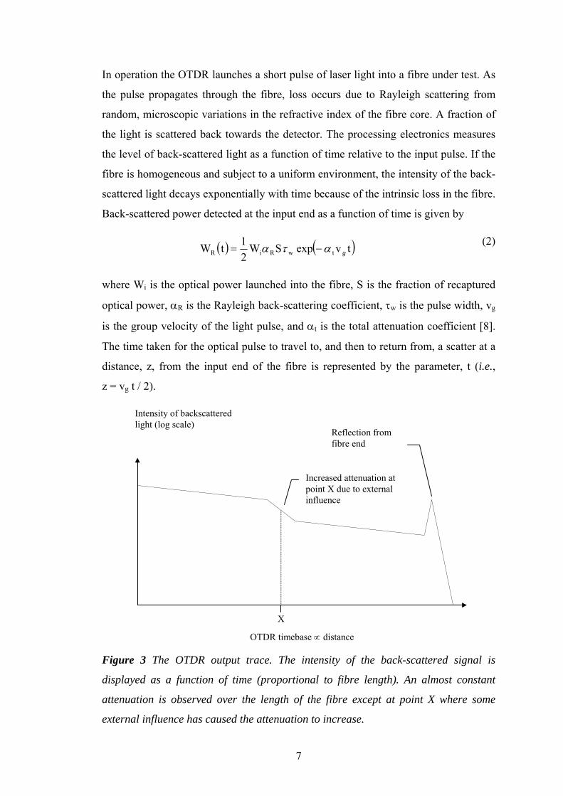
Figure 3 The OTDR output trace. The intensity of the back-scattered signal is
displayed as a function of time (proportional to fibre length). An almost constant
attenuation is observed over the length of the fibre except at point X where some
external influence has caused the attenuation to increase.
OTDR timebase ∝ distance
X
Reflection fromfibre end
Increased attenuation atpoint X due to externalinfluence
Intensity of backscatteredlight (log scale)
8
The exponential term represents the fibre attenuation characteristics. It is assumed
that the loss experienced by the back-scattered signal and the forward pulse are equal.
Hence, the slope of the logarithm of this detected signal is equal to the loss coefficient
at location z:
( )d Wdz
Rt
ln= −2α
(3)
Regions of high loss are indicated by an increase in the slope of the OTDR trace, as
shown in figure 3. Spatial resolution is determined by the input pulse width:
∆zvg w
min =τ
2
(4)
However, the low energy associated with short pulses results in a restricted range [9].
In short, the OTDR is a fibre optic sensor that inherently measures attenuation as a
function of distance. It has proven itself to be an invaluable diagnostic tool in the
telecommunication industry, being used for the detection of fibre damage and
measurement of fibre performance.
2.4 Practical Considerations
For long-distance, high-bandwidth communications, monomode fibres are preferred
to the multimode type, despite having a core diameter of just 5 µm compared with a
more manageable 50 - 60 µm for multimode fibres [9]. However, they have the
attraction that there is no differential mode dispersion7 so the available bandwidth can
be very high.
7 Differential mode dispersion results from the different paths, or modes of propagation, available to light in
multimode fibre. For a single wavelength of light and a uniform refractive index, every ray travels at the same
speed but arrives at different times. This effect is mitigated by using ‘graded index fibre’, where the core is
made of concentric layers of glass of varying refractive index. Rays propagating further from the axis of the
fibre, and so travelling a longer path, spend most of their journey in glass of a lower refractive index than rays
propagating closer to the axis. Therefore, rays which travel a longer distance also travel faster and arrive at
roughly the same time as those that travel a shorter distance.
9
The maximum resolution of an OTDR system is limited by chromatic dispersion8
which depends on the linewidth of the source. A dispersion of just a few ns km-1
generates an error in the distance measurement of some tens of metres for a 100 km
length of cable. (Chromatic dispersion is a major problem for extremely long-distance
(> 1 000 km), high-bandwidth cables [4]. Current research in the use of soliton pulses
that maintain their shape as they propagate through the medium, and wavelength
division multiplexing that makes optimum use of available bandwidth, is seeking to
overcome this limitation.)
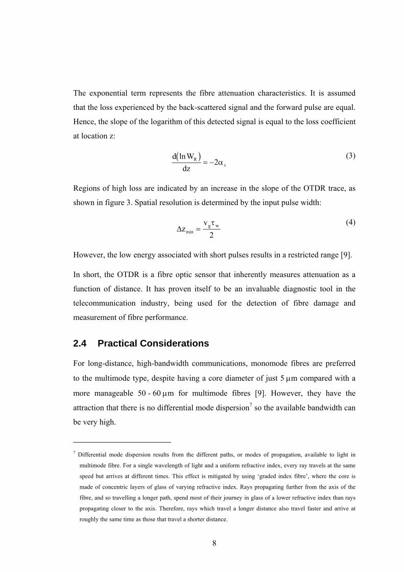
Contaminating elements in glass, introduced during the manufacturing process,
absorb energy from incident light. The amount of energy absorbed depends on the
proportion of impurity atoms present. Absorption produced by transition metals is
strongly dependent on frequency and can be avoided by choosing a suitable
wavelength for the light source. The other main absorption mechanism is due to the
presence of the hydroxyl ion, OH-, which has a pronounced absorption peak at
2 800 nm and the harmonics 1 400 nm, 970 nm and 750 nm. The position of the peaks
can be seen clearly in the frequency-attenuation curve shown in figure 4.
The 800 - 900 nm band is popular for low-cost, short-haul systems. A better choice
for telecommunication is the 1 300 nm minimum dispersion wavelength. However,
most modern long-distance systems use the narrow window around the 1 550 nm
minimum absorption wavelength.
OTDR measurements are further complicated by the conditions at the fibre break.
Fibre ends which have been snapped or broken cause random dispersion of light,
limited only by the numerical aperture. A reflecting, complete break appears as a clear
discontinuity in the back-scatter profile and is the easiest fault to detect. Conversely, a
non-reflecting, partial break is the most difficult to detect since the change in back-
scatter power level may be very small [9].
8 Chromatic, or normal, dispersion occurs because different frequencies of light propagate through a medium at
different speeds. In general, at shorter wavelengths the ‘phase speed’ of light in a medium is less than at longer
wavelengths. Therefore, the shorter wavelengths in a pulse of light in an optic fibre will travel more slowly than
the longer wavelengths, causing the pulse to spread out in time. The effect is mitigated by using a light source
with a narrow spectral linewidth.
10
Figure 4 The characteristic optical attenuation spectrum of glass optic fibres [10].
Finally, microbending losses can affect the accuracy of an OTDR loss measurement.
It is well known that dielectric waveguides lose power by radiation if their axes are
curved (as noted in section 3.3 of the first report in this series1). Marcuse derived a
curvature loss formula for optic fibres by expressing a general solution of Maxwell’s
equations for the field outside the fibre as a superposition of cylindrical outgoing
waves [11, 12].
It is not possible to determine whether the losses measured by an OTDR are caused
by absorption or radiation from bends. Submarine telecommunication cable is usually
laid in a straight line, only deviating to avoid seafloor hazards, so bending losses do
not cause much of a problem. However, this loss mechanism can severely limit the
effectiveness of an OTDR in distributed sensing applications. Sensors which make
use of non-linear optical effects are able to give much less ambiguous measurements.
11
3 Non-Linearity in Fibre Transmission
Non-linear processes in monomode, optic fibre transmission systems have been
referred to, briefly, in section 2. There are four important processes to consider:
Raman scattering; Brillouin scattering; self-phase modulation; and parametric, four-
photon mixing [13]. These can lead to signal loss, pulse spreading, crosstalk and even
physical damage to the optic fibre.
• Raman Scattering. This process occurs under the influence of focused, high-
energy laser pulses. The back-scattered signal consists of light of the same
frequency and weak, sideband components. The difference between these
sidebands and the incident frequency is characteristic of the vibrational modes of
molecules in the material [14, 15].
• Brillouin Scattering. This results from the interaction between light and thermally
generated acoustic waves in the medium. The acoustic wave produces density
variations which result in a periodic modulation of the material dielectric constant.
Scattered light is, effectively, Doppler-shifted by the movement of the acoustic
wave [15, 16]. This process will be detailed in section 3.1.
• Self-Phase Modulation. This is a broadening of the signal spectrum at high
intensities which, in turn, causes pulse spreading through chromatic dispersion
[13]. (In passing, it should be noted that different pulse waveforms, such as soliton
pulses [17], can cause intensity dependent pulse narrowing which decreases the net
broadening from group-velocity dispersion.)
• Four-Photon Mixing. This is a parametric interaction between light of different
frequencies which generates new frequencies on either side of the pump frequency
[13]. This is not a serious problem in transmission systems because of the need for
phase matching in single-mode fibres and high powers in multimode fibres.
The extremely low-loss fibres and high-power, narrow-linewidth lasers used in
submarine cable systems make non-linear effects important. In monomode fibres
these effects can appear at optical powers of only a few milliwatts. However, fibre
non-linearities have enormous potential for distributed sensing applications.
12
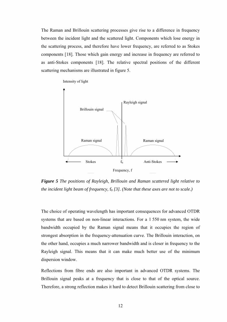
The Raman and Brillouin scattering processes give rise to a difference in frequency
between the incident light and the scattered light. Components which lose energy in
the scattering process, and therefore have lower frequency, are referred to as Stokes
components [18]. Those which gain energy and increase in frequency are referred to
as anti-Stokes components [18]. The relative spectral positions of the different
scattering mechanisms are illustrated in figure 5.
Figure 5 The positions of Rayleigh, Brillouin and Raman scattered light relative to
the incident light beam of frequency, f0 [3]. (Note that these axes are not to scale.)
The choice of operating wavelength has important consequences for advanced OTDR
systems that are based on non-linear interactions. For a 1 550 nm system, the wide
bandwidth occupied by the Raman signal means that it occupies the region of
strongest absorption in the frequency-attenuation curve. The Brillouin interaction, on
the other hand, occupies a much narrower bandwidth and is closer in frequency to the
Rayleigh signal. This means that it can make much better use of the minimum
dispersion window.
Reflections from fibre ends are also important in advanced OTDR systems. The
Brillouin signal peaks at a frequency that is close to that of the optical source.
Therefore, a strong reflection makes it hard to detect Brillouin scattering from close to
Rayleigh signal
Raman signal Raman signal
f0
Frequency, f
Anti-StokesStokes
Brillouin signal
Intensity of light

13
the end of the fibre. Conversely, the peak of the Raman signal is much further from
the source frequency. This means that low loss and low crosstalk separation between
the input optical pulse and the back-scattered light pulse can be realised. However,
the Raman signal has the disadvantage of a very weak return which is around 30 dB
below the Rayleigh signal.
Brillouin scattering has certain advantages over Raman scattering when used for the
detection of strain variations over long lengths of optic fibre (i.e., lengths in excess of
100 km). These advantages are noted in section 4. Raman scattering will not be given
any further consideration in this series of reports. A physical description of Brillouin
scattering is presented in the following section. In section 5, the related acousto-optic
effect is also presented, and an experiment is described in section 6 to test the
feasibility of using an OTDR to detect acoustically generated stresses in an optic
fibre.
3.1 Brillouin Scattering
Brillouin scattering is of particular interest in this application since, not only is the
intensity of spontaneous scattering dependent on temperature, but its frequency is
dependent on both temperature and strain. Hence, the Brillouin frequency shift is a
mechanism for detecting pressure variations generated by a probing acoustic beam.
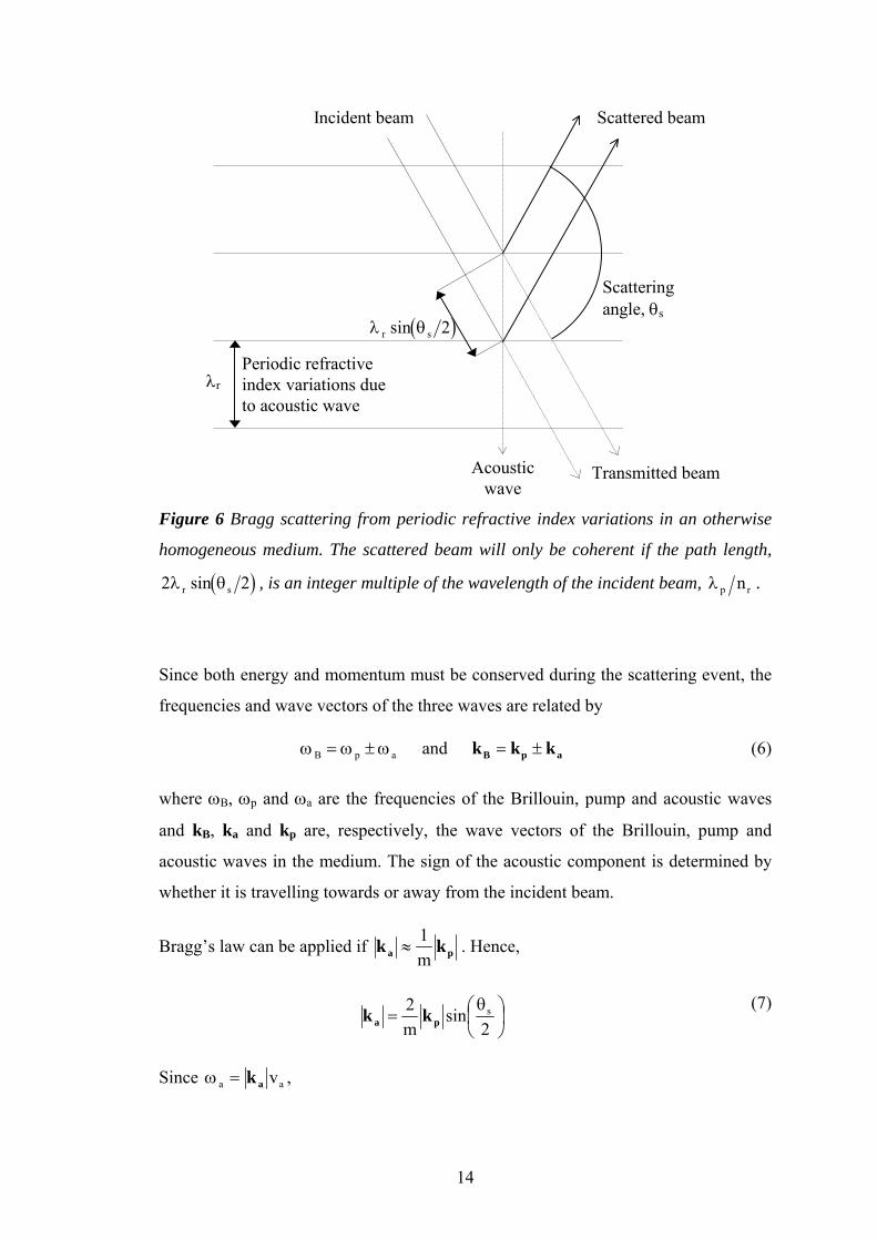
The modulation of the dielectric constant can cause the incident light beam to be
reflected according to Bragg’s law. This states that constructive interference takes
place if the wavelength of the acoustic modulation, λr, is related to the wavelength of
the incident light (or ‘pump’) in the medium, λp / nr, by
pr
sr
mλλ =
θ2n sin2
⎛ ⎞⎜ ⎟⎝ ⎠
(5)
where m is a positive integer which allows for higher order scattering, and θs is the
angle between the incident and scattered waves, as shown in figure 6. Note that λp is
the ‘free space’ wavelength of the pump source.
14
Figure 6 Bragg scattering from periodic refractive index variations in an otherwise
homogeneous medium. The scattered beam will only be coherent if the path length,
( )2 2λ θr ssin , is an integer multiple of the wavelength of the incident beam, λ p rn .
Since both energy and momentum must be conserved during the scattering event, the
frequencies and wave vectors of the three waves are related by
ω ω ωB p a= ± and k k kB p a= ± (6)
where ωB, ωp and ωa are the frequencies of the Brillouin, pump and acoustic waves
and kB, ka and kp are, respectively, the wave vectors of the Brillouin, pump and
acoustic waves in the medium. The sign of the acoustic component is determined by
whether it is travelling towards or away from the incident beam.
Bragg’s law can be applied if k ka p≈1m
. Hence,
⎟⎠⎞
⎜⎝⎛ θ=
2sin
m2 s
pa kk (7)
Since ω a av= k a ,
Scattered beamIncident beam
Transmitted beamAcousticwave
Periodic refractiveindex variations dueto acoustic wave
λr
( )λ θr ssin 2
Scatteringangle, θs

15
⎟⎠⎞
⎜⎝⎛ θ=ω
2sinv
m2 s
aa pk (8)
The Brillouin shift, ωS, is the difference between the frequencies of the incident light
and the scattered light. Equation (6) indicates that this equal to the acoustic frequency,
ωa. Given kp =2πλ
nr
p
,
ωπλ
θS
r a
p
sn vm
= ± ⎛⎝⎜
⎞⎠⎟
42
sin (9)
In the forward direction (θs = 0), the frequency shift is zero. Light scattered in this
direction is coincident with, and therefore indistinguishable from, the incident light.
Only the back-scattered light (θs = π), which has a Brillouin frequency shift of
4π λn vr a p , has any significance.
The Brillouin scattering coefficient, αB is similar in form to the Rayleigh back-
scattering coefficient. However, as the scattering is from thermally generated moving
acoustic waves instead of frozen in fluctuations, there is a proportional dependence on
temperature, Tabs.
( )απλ
κ ρB r EM abs g an p T v=−8
3
3
48 2 2 1
(10)
The ratio of the Rayleigh to Brillouin scatter is known as the Landau-Placzek ratio,
LPR [3]. From equations (1) and (10),
( )LPR TT
vf
absT g a= −β ρ 2 1 (11)
At a temperature of 4 °C, and using the values given in section 2.2, LPR is 20.8.
Therefore, each of the two Brillouin components (Stokes and anti-Stokes) is
approximately 16 dB below the Rayleigh signal.
Above a certain threshold power, the back-scattered light extracts energy from the
incident pump beam and so experiences a process of amplification. The effect is then
no longer spontaneous but is said to be stimulated Brillouin scattering (SBS). As SBS

16
grows from what is originally a spontaneous signal, its frequency also has a
temperature and strain dependence [3].
4 Brillouin Back-Scatter Systems
The principle of operation of the Brillouin optical fibre sensor is similar to that of the
OTDR, the main difference being that the scatter mechanism is Brillouin instead of
Rayleigh. Hence the term ‘Brillouin OTDR’ (BOTDR) is used [19].
There are two important practical differences: a narrow linewidth source must be used
so that the Rayleigh back-scatter does not mask the Brillouin signal; and the Brillouin
back-scatter must be separated from the Rayleigh back-scatter at the detector using
some form of filter. For a distributed temperature sensor, all that is required is to
analyse the intensity of the back-scattered Brillouin signal as a function of time. If
both the intensity and frequency of the back-scattered light are analysed it is possible
to implement a combined distributed temperature and strain sensor.
It should be noted that Raman OTDRs are also in common use. However, the
Brillouin effect offers a number of advantages over the Raman effect for distributed
sensing [3]:
• The back-scatter intensity is an order of magnitude higher than that of Raman and,
therefore, provides the possibility of greater range.
• Owing to the small frequency shift between the incident and back-scattered light,
maximum advantage may be taken of the low attenuation window at 1 550 nm.
• The Brillouin signal may be recovered by optically heterodyning the back-
scattered signal with a reference signal, resulting in a more convenient frequency
for signal processing.
The disadvantages associated with Brillouin back-scatter sensors are a reduced
sensitivity to temperature and difficulty in separating the Brillouin and Rayleigh
signals due to their small frequency separation.
The dependency of the Brillouin shift on variations in temperature and strain are
summarised in the following sections. The strain dependence is of particular interest

17
in this study, since acoustic waves incident on an optic fibre should give rise to a
variation in strain. The temperature dependence is presented for completeness.
4.1 Temperature Dependence of the Brillouin Shift
The refractive index and the velocity of acoustic waves both vary as a function of
temperature. The two effects are additive, but the contribution by the acoustic velocity
variation is, by far, the dominant one. The velocity of acoustic waves in the fibre is
given by
( )( )( )
vE
aY
g
=−
+ −1
1 1 2ν
ν ν ρ
(12)
where EY is Young’s modulus, ν is Poisson’s ratio and ρg is the density of the glass
[20]. Young’s modulus and density vary as a function of temperature. However, the
temperature coefficient of volume expansion is very small (around 2.5 × 10⁻⁶ / °C
[21]) so density can be assumed to remain constant. In the range 0 - 200 °C the optical
frequency variation is approximately 1 MHz / °C.
4.2 Strain Dependence of the Brillouin Shift
When a material is deformed, e.g., by an acoustic wave, there is a change in refractive
index, ∆nr, which is related to the applied axial strain, εz, by
( )[ ]∆n n p prr
z EM z EM= − − −3
11 1221ε ν ε ν
(13)
where pEM11 and pEM12 are the {1,1} and {1,2} elements respectively of the elasto-
optic coefficient tensor9 [22]. (Axial (εz) and radial (εr) strains are related through
Poisson’s ratio by, ν ε ε= − r z [23]).
9 When a material is formed, its optical properties change due to strain Skl. This is known as the
elasto-optic or acoustic-optic effect. The latter name is given because, in practice, the strain is usually
produced by a propagating acoustic wave, often at ultrasonic frequencies.
klijklij Sp=∆η (f.1)
18
Since Poisson’s ratio, ν, and Young’s modulus, EY, are also dependent on strain, the
variation of acoustic velocity must also be considered [24]. The effects of refractive
index and acoustic velocity are usually in opposition, but the acoustic velocity
variation is dominant. By substituting equations (12) and (13) into equation (9), the
formula for the Brillouin frequency shift, an expression for the frequency-strain
sensitivity of an optic fibre can be deduced [3].
The radial sensitivity of a typical glass fibre is around 9 kHz / µstrain. This
corresponds to an applied stress, or pressure, sensitivity of approximately
130 Hz / kPa (given that the Young’s modulus of glass is around 7 × 10¹⁰ Pa [25]).
Even with a sensitive interferometric system this modulation would be very hard to
detect, given that the optical frequencies are in the terahertz band.
The related acousto-optic effect is investigated in the following section. It will be seen
that the pressure sensitivity equation includes a term that is similar to equation (14).
However, the acousto-optic effect also takes into account the physical change in the
length of the fibre, which may result in a much higher sensitivity.
5 Optic Fibre Hydrophones
A variety of optic fibre hydrophone systems, that take advantage of the acousto-optic
effect, have been developed in recent years [26]. The most successful are those based
on interferometry [27]. In such systems the change in relative phase between a light
beam injected into a fibre and the same beam exiting the fibre is measured. This phase
change is caused by changes in physical length and refractive index which are directly
where pijkl is the elasto-optic coefficient tensor. Noting that ijη∆ and Skl are both rank 2 symmetric
tensors, we can rewrite (f.1) in abbreviated subscript notation as
JIJI Sp=∆η (f.2)
ijklIJijI pp =∆=∆ ,ηη (f.3)
The variable pIJ represents the elasto-optic (or acoustic-optic) coefficient matrix.

19
related to changes in pressure. The advantage of using an interferometric system is
that a very high sensitivity can be achieved10.
The total phase change is the sum of many small changes which are accumulated as
the incident light is transmitted. However, in this application, access is only available
to one end of the fibre. Therefore, to measure the change in phase, light must be
returned from the far end. This is possible if the break in the fibre is reflective; light
will be returned along the same path, experiencing twice the phase change. However,
in the case of a non-reflecting, partial break, it may not be possible to implement this
kind of sensor [9].
The phase delay of an optical signal propagating at speed, cg, in a fibre of length, l, is
grad clω=φ . Hence, the pressure sensitivity of the optical phase in a fibre can be
defined as 0radrad p∆φφ∆ , where ∆φrad is the shift in phase due to a pressure change,
∆p0. If this pressure change results in a fibre core axial strain, εz, and a radial strain,
εr, it has been shown that [29]
( )[ ]∆φ rad
radz
rr EM EM z EM
n p p pφ
ε ε ε= − + +2
11 12 122
(14)
The first term represents the physical length change in the fibre. The second term is
similar to equation 14, and represents the refractive index modulation of the core.
These are frequently in opposition, but the physical length change is usually the more
important effect.
Practical optic fibres comprise a glass core surrounded by layers, which are also made
of glass, with an outer jacket of plastic. In a telecommunication cable several fibres
are bundled together to form a single fibre unit which is, itself, sheathed in layers of
insulation, armour, etc. (see section 2.1 of the first report in this series1). However, an
understanding of the physical processes at work can be obtained from a model of a
10 An example of the sensitivity that can be achieved with an interferomteric system is the measurement of the SI
unit of length. The metre is defined as being 1 650 763.73 wavelengths of a particular line in the spectrum of
krypton in a vacuum. The measurement required to set up this standard involves forming an interference pattern
between two mirrors, and counting the number of fringes which cross the field of view as one mirror is moved
relative to the other. The movement of 1/10 of a fringe can just be detected, so the accuracy attainable is about 1
part in 107 [28].

20
single, multi-layered fibre. Hughes and Jarzynski derived a complete three-
dimensional model of the strains in such a fibre [20, 30].
These researchers have also shown that a much simpler ‘plane-strain’ model, which
requires significantly less computation, can be used. This was found to be in good
agreement with the three-dimensional model (within 1.5 % for a typical three layer
fibre), with the accuracy reducing as the number of layers was increased. A
mathematical description of the plane-strain model and its relationship to the pressure
sensitivity (equation (14)) is presented in Appendix A.
The elastic and elasto-optic coefficients are not generally known for the variety of
glasses used for optic fibres. Previous studies of the sensitivity of high silica content
fibres have assumed that they were equal to those of fused silica [31]. In this study,
however, data was made available by Cable & Wireless for a typical monomode fibre.
Parameters for the core and three layers are presented in table 1.
Fibre Parameter Core Layer 1 Layer 2 Layer 3
Composition SiO2
GeO2 (trace)
SiO2 (95 %)
B2O3 (5 %)
SiO2 Silicone
Radius (µm) 2 13 42 125
Young’s modulus (GPa) 72 65 72 0.0035
Poisson’s ratio 0.17 0.149 0.17 0.49947
pEM11 0.126 - - -
pEM12 0.27 - - -
Refractive index 1.458 - - -
Table 1 The composition, dimensions and elastic and elasto-optic coefficients of a
typical single mode optic fibre.
21
Figure 7 Calculated pressure sensitivity as a function of fibre radius. The different
curves are for outer jacket layers with different Young's moduli, EY. The bulk
modulus, Kb, was kept the same (4 GPa) in each case.
The sensitivity of this fibre was investigated using the plane-strain model. A
hydrostatic boundary condition was chosen, this being the most appropriate for a long
fibre. An outer jacket, layer four, was included. The radius and Young’s modulus of
this layer was varied while the bulk modulus, Kb, was fixed at a value of 4 GPa. The
set of pressure sensitivity curves that resulted from these calculations are shown in
figure 7.
As the coating gets very thick the pressure sensitivity approaches a limit which is
independent of the Young’s moduli. This suggests that for very thick coatings the
magnitude of the strains in the fibre are dependent on the bulk moduli alone. Figure 8
confirms this to be the case. In this calculation the radius of the outer layer was fixed
at 3 mm and Young’s modulus set at 0.1 GPa. The curve is inversely proportional to
the bulk modulus, i.e., linear with the compressibility, of the outer layer. At smaller
radii the sensitivity relationship is more complicated, being a function of changes in
both elastic moduli.
22
Figure 8 Calculated pressure sensitivity as a function of bulk modulus, Kb, for a large
radius (3 mm) outer jacket. Young’s modulus, EY, was kept constant (0.1 GPa).
These results demonstrate that a greatly enhanced pressure sensitivity can be achieved
using a clad, rather than an unclad, fibre [32]. This can be further improved by using a
coating with a high compressibility, which is precisely the case for non-metallised
fibre optic cables. It has been demonstrated that fibres with metal cladding layers are
much less sensitive than fibres clad with low bulk modulus materials [33]. Non-
metallised submarine telecommunication cables may be particularly suited to
detection by this method.
6 OTDR Experiment
The feasibility of using a conventional OTDR to detect acoustically generated stresses
in an optic fibre was investigated. The purpose of this investigation was to determine
whether an OTDR, of the kind that is commonly used in the telecommunication
industry, could be applied directly to the cable detection problem.

23
The particular device that was used (an Anritsu MW9070A OTDR) exhibited an
optical bandwidth of around 60 nm [34]. That is to say, at an optical wavelength of
1 550 nm the optical bandwidth of the OTDR would have been around 5 THz. This is
much greater than the Brillouin frequency shift in silica which is ± 11 GHz.
Therefore, it should be noted that this device was not capable of isolating Brillouin
back-scattered signals from the back-scattered Rayleigh signal since its output would
have encompassed all the back-scattered signals that existed within the optical
bandwidth.
The apparatus is depicted in figure 9. The OTDR was connected to a 1.8 km length of
monomode optic fibre. The properties of this fibre were similar to those of the fibre
presented in table 1. The outer jacket was made of acrylic and the overall diameter
was around 1 mm. The end of the fibre was clipped to give a strong reflection, which
was easy to identify in the OTDR back-scatter trace. The acoustic source was
purpose-built using a piezo-ceramic tube transducer encapsulated in a light-duty
epoxy resin.
Figure 9 The apparatus used in the OTDR experiment. The OTDR was connected to a
1.8 km length of optic fibre wound on a mandrel. The final 8 m of fibre was wound
through a submerged tubular acoustic source. The fibre was excited using the
acoustic source, and the back-scattered optical signal was measured using the OTDR.
24
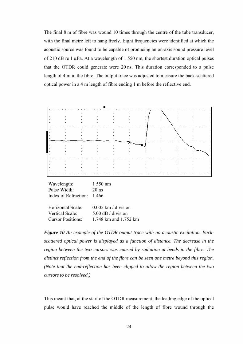
The final 8 m of fibre was wound 10 times through the centre of the tube transducer,
with the final metre left to hang freely. Eight frequencies were identified at which the
acoustic source was found to be capable of producing an on-axis sound pressure level
of 210 dB re 1 µPa. At a wavelength of 1 550 nm, the shortest duration optical pulses
that the OTDR could generate were 20 ns. This duration corresponded to a pulse
length of 4 m in the fibre. The output trace was adjusted to measure the back-scattered
optical power in a 4 m length of fibre ending 1 m before the reflective end.
Wavelength: 1 550 nmPulse Width: 20 nsIndex of Refraction: 1.466
Horizontal Scale: 0.005 km / divisionVertical Scale: 5.00 dB / divisionCursor Positions: 1.748 km and 1.752 km
Figure 10 An example of the OTDR output trace with no acoustic excitation. Back-
scattered optical power is displayed as a function of distance. The decrease in the
region between the two cursors was caused by radiation at bends in the fibre. The
distinct reflection from the end of the fibre can be seen one metre beyond this region.
(Note that the end-reflection has been clipped to allow the region between the two
cursors to be resolved.)
This meant that, at the start of the OTDR measurement, the leading edge of the optical
pulse would have reached the middle of the length of fibre wound through the

25
acoustic source. The trailing edge of the pulse would have just entered this region of
the fibre. Similarly, at the finish of the OTDR measurement, the leading edge of the
pulse would have reached the end of the wound length of the fibre. The trailing edge
would have reached the middle of this region of the fibre. Hence, throughout the 4 m
OTDR measurement window, the optical pulse would have resided entirely within the
region of fibre that could have been excited by the acoustic source.
Figure 11 Two sets of data (+, ×) showing back-scattered optical power in decibels as
a function of the acoustic excitation frequency. The values were calculated relative to
the back-scattered optical power in the case when there was no acoustic excitation. A
best-fit curve for the combined data sets is shown by the solid curve.
An example of the OTDR output trace is shown in figure 10. In the case shown the
fibre was not excited by the acoustic source. The back-scattered power in the
measurement region (between the two cursors) reduces at a significantly greater rate
than in the fibre before this region. The increase in loss is due to the radiation of

26
optical power from the bends in the section of fibre wound through the tube
transducer.
The back-scattered optical signal was measured with no acoustic excitation and with a
210 dB re 1 µPa excitation at each of the output frequencies. In order to be certain of
a statistically significant result, 1 000 averages of the signal were performed in each
case. The measurements were then repeated to check that they were consistent.
Under the influence of an acoustic field, the back-scattered optical power was
observed to increase over the OTDR measurement window. Changes in back-scatter
as a function of acoustic frequency for the two sets of measurements are presented in
figure 11. In this instance, ‘change’ is defined as being the difference, in decibels,
between the measurements with and without acoustic excitation. In other words, the
figure shows the back-scattered optical power measured in decibels relative to the
back-scattered optical power with no acoustic excitation.
It was expected that the coupling between the fibre and the acoustic field would
improve as the acoustic wavelength decreased, implying that the back-scattered
optical power should increase with frequency. This is consistent with the change that
was observed. That is to say, the data points in figure 11 tend, asymptotically, towards
a maximum value at high frequencies. A simple model that is consistent with this
behaviour is the sigmoid:
( )W a
b cfdBk
=+ −1 exp
(15)
where WdB is the optical back-scatter relative to the case when there was no acoustic
excitation, and fk is the acoustic frequency in kHz. A linear regression was performed
for the data presented in the graph, resulting in the following values for the three
fitting parameters11: a = 0.433 dB; b = 24.8; and c = 0.0753 s. The standard error on
the curve model was estimated to be 0.10 dB.
11 Linear regression algorithms attempt to produce models having the least standard error between themselves and
the data. They do not automatically produce error estimates. However, examination of a family of fitted curves
27
A model of this form could be applied to measurements performed on a real
telecommunication cable in the future. If combined with the attenuation spectra of the
ocean and the seabed, an optimum acoustic operating frequency could be determined
in a similar way to the determination of the optimum frequency band (detailed in
section 3.2 of the fourth report in this series4). It is expected that the optimum
frequency would coincide with the geometry of the cable, i.e., ka t = 1 . However, this
supposition is subject to experimental verification in the marine environment.
This result has confirmed that acoustically generated stresses can cause a change in
the back-scattered optical power, as measured using a conventional OTDR. However,
the observed change was found to be very small (i.e., the change in optical power was
around 0.5 dB for a sound pressure level of 210 dB re 1 µPa).
Therefore, it has been concluded that for a cable detection system of this kind to be
successful, a specially designed OTDR would be required (such as an OTDR
designed to measure the Brillouin shift, or a sensitive interferometric system designed
to measure changes in phase).
7 Summary
An alternative to the remote acoustic approach to the detection of buried objects has
been considered for the special case of buried fibre optic communication cables. It
was the aim of this report to investigate the theory surrounding such a system, and to
assess the feasibility of its practical use.
The use of optic fibres as distributed sensors has been discussed. The most notable
example of such a system is the OTDR. Non-linear optical processes that could be
exploited in a distributed sensor have also been discussed. The Brillouin effect was
given special consideration. It was noted that the associated Brillouin frequency shift
depends on variations in temperature and, of particular interest, variations in strain.
The related, acousto-optic effect, was investigated in section 5. It was shown that both
length and refractive index changes (in response to an applied strain) can cause a
suggests that the stated errors in the parameters a, b and c are, respectively, ± 0.1, ± 5, and ± 0.02. Hence, the 3
significant figures to which the fitted parameters are quoted should be viewed with caution.

28
change in the optical phase within a fibre. Moreover, pressure sensitivity was shown
to be related to the elastic properties of the fibre jacket material. A greatly enhanced
sensitivity is predicted if the cladding has a high compressibility (which is expected to
be the case for non-metallised fibre optic cables).
An experiment was performed to investigate whether a conventional OTDR could be
used to detect acoustically-generated stresses within an optic fibre. A change in the
back-scattered power in the optical window of the detector was found to occur. A
simple curve model, conforming to the expected behaviour of the system, was
subsequently fitted to the experimental data.
In the experiment (detailed in section 6) the change that was observed was very small.
It was concluded that an OTDR system, specifically designed to pick out the Brillouin
frequency shift, or an interferometric system designed to pick up small changes in
optical phase, would be required for the acousto-optic detection approach to work in
practice.
The strain dependence of the Brillouin shift (section 4.2) was estimated to be around
130 Hz / kPa. At optical wavelengths of around 1 500 nm in glass, this corresponds to
a change in the phase of the Brillouin signal (∆φrad / φrad ∆p0) of only 10-15 Pa-1. For
the acousto-optic effect, the change in phase of the optical signal was expected to be
significantly larger (see section 5). For a fibre having a relatively thick and
compressible cladding, it was calculated to be of the order of 10-10 Pa-1.
The sensitivity values for a real fibre optic cable buried in marine sediment are
unknown, although they are expected to be similar to the values predicted (above) for
the Brillouin and acousto-optic effects. Therefore, it is surmised that an acoustic
pressure amplitude in excess of 100 kPa would be required to be incident on the cable
to achieve a measurable effect12, given that a sensitivity of around 1 part in 107 can be
achieved using interferometric techniques.
This area of study has been taken as far as possible with the laboratory facilities that
were made available. However, there are still a number of questions that need to be
12 There exist experimental sources, capable of generating acoustic pressures high enough to remotely detonate
underwater mines [35]. However, little has been published regarding their effective range, directivity or
frequency response characteristics.

29
resolved. In particular, the acoustic pressure amplitude required to produce a
measurable effect in a cable buried in sand has not been measured. This may form the
basis of a future study if the acousto-optic detection technique is ever considered for
use in the field.
This material formed the basis of the PhD of RCPE [36-39].
30
APPENDIX A
OPTIC FIBRE PRESSURE SENSITIVITY
A.1 Calculation of Pressure Sensitivity
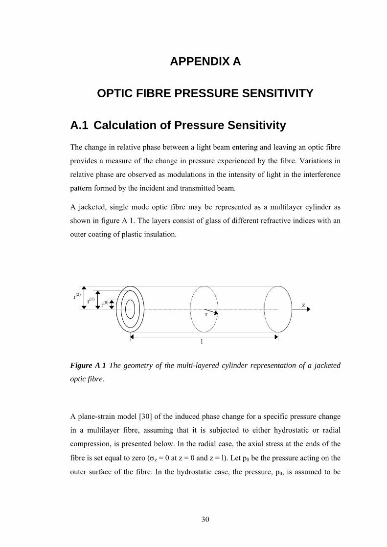
The change in relative phase between a light beam entering and leaving an optic fibre
provides a measure of the change in pressure experienced by the fibre. Variations in
relative phase are observed as modulations in the intensity of light in the interference
pattern formed by the incident and transmitted beam.
A jacketed, single mode optic fibre may be represented as a multilayer cylinder as
shown in figure A 1. The layers consist of glass of different refractive indices with an
outer coating of plastic insulation.
r(0)r(1)r(2)
rz
l
Figure A 1 The geometry of the multi-layered cylinder representation of a jacketed
optic fibre.
A plane-strain model [30] of the induced phase change for a specific pressure change
in a multilayer fibre, assuming that it is subjected to either hydrostatic or radial
compression, is presented below. In the radial case, the axial stress at the ends of the
fibre is set equal to zero (σz = 0 at z = 0 and z = l). Let p0 be the pressure acting on the
outer surface of the fibre. In the hydrostatic case, the pressure, p0, is assumed to be

31
applied uniformly to the fibre. Therefore, the axial stress at the ends is - p0. In either
case, axial symmetry is assumed.
Polar stresses in the fibre are related to the strains as follows:
( )
( )
( )
( ) ( ) ( ) ( )
( ) ( ) ( ) ( )
( ) ( ) ( ) ( )
( )
( )
( ) ⎥⎥⎥
⎦
⎤
⎢⎢⎢
⎣
⎡
εεε
×⎥⎥⎥
⎦
⎤
⎢⎢⎢
⎣
⎡
µ+λλλλµ+λλλλµ+λ
=⎥⎥⎥
⎦
⎤
⎢⎢⎢
⎣
⎡
σσσ
θθi
z
i
ir
iiii
iiii
iiii
iz
i
ir
22
2
(A 1)
where the σ terms are stresses, the ε terms are strains and the subscripts, r, θ and z,
relate to the radial, torsional and axial components. The index, i, denotes the fibre
core layer where i = 0 is the core. The Lamé parameters [20], λ and µ, are related to
the Young’s modulus, EY, and Poisson’s ratio, ν, of the fibre by,
( )( ) ( )
( )( ) ( )( )( )
( )
( )( )i
iYi
ii
iY
ii
12E
; 211
Eν+
=µν−ν+
ν=λ
(A 2)
For a cylinder, the strains can be obtained from the Lamé solutions,
( ) ( )( )
( ) ( )( )
( ) ( )i0
iz2
i1i
0i
2
i1i
0i
r W ; r
UU ;
rU
U =ε−=ε+=ε θ (A 3)
where U0(i), U1
(i) and W0(i) are the parameters that must be determined to find the
strains at the radius, r. Since the strains must be finite at the centre of the core,
U1(0) = 0. Also, since the axial strain must be, in effect, the same for every layer in the
fibre, the parameter, W0(i), simply becomes W0.
Expanding equation (A 1) gives
( ) ( ) ( )( ) ( ) ( ) ( ) ( ) ( )
( ) ( ) ( ) ( ) ( )( ) ( ) ( ) ( )
( ) ( ) ( ) ( ) ( ) ( ) ( )( ) ( )iz
iiiiir
iiz
iz
iiiiir
ii
iz
iiiir
iiir
2
2
2
εµ+λ+ελ+ελ=σ
ελ+εµ+λ+ελ=σ
ελ+ελ+εµ+λ=σ
θ
θθ
θ
(A 4)

32
and substituting the Lamé solutions from equation (A 4),
( ) ( ) ( )( ) ( )( )
( ) ( )( )
( )
( ) ( ) ( )( )
( ) ( )( ) ( )( )
( )
( ) ( ) ( )( )
( ) ( )( )
( ) ( )( )
σ λ µ λ λ
σ λ λ µ λ
σ λ λ λ µ
θ
ri i i i
ii i
ii
i i ii
i i ii
i
zi i i
ii i
ii i
U Ur
U Ur
W
U Ur
U Ur
W
U Ur
U Ur
W
= + +⎛
⎝⎜
⎞
⎠⎟ + −
⎛
⎝⎜
⎞
⎠⎟ +
= +⎛
⎝⎜
⎞
⎠⎟ + + −
⎛
⎝⎜
⎞
⎠⎟ +
= +⎛
⎝⎜
⎞
⎠⎟ + −
⎛
⎝⎜
⎞
⎠⎟ + +
2
2
2
012 0
12 0
012 0
12 0
012 0
12 0
(A 5)
Under the assumption that radial pressure is uniform, there is no torsional stress
component so σr(i) = σθ
(i). By equivalence of the terms in equation (A 5) and setting ( )U
r10
2 0= ,
( ) ( ) ( )( ) ( )( ) ( )
( )
( ) ( ) ( ) ( ) ( )( )σ λ µ
µλ
σ λ λ µ
ri i i i
i ii
zi i i i i
U Ur
W
U W
= + + +
= + +
2 2
2 2
01
2 0
0 0
(A 6)
The radial (u(i)) and axial (w(i)) displacements are obtained from the Lamé solutions,
( ) ( )( )
( )u U r Ur
W zi ii
i= + =01
0 ; w (A 7)
To solve equation (A 3) it is necessary to establish a set of boundary conditions. For a
fibre with n layers, the continuity of stress at each layer boundary is

33
( )( )
( )( )σ σr
i
r r ri
r ri in
=
−
== = −1 1 1 ; i K (A 8)
and the continuity of displacement at each layer boundary is
( )( )
( )( )u u nr
i
r r ri
r ri i=
−
== = −1 1 1 ; i K (A 9)
The radial stress on the outer layer of the fibre is
( )n-1r 0σ =-p (A 10)
where p0 is the pressure acting on the outer surface of the fibre.
An effective axial strain is chosen so that the net axial force, F, satisfies the boundary
conditions at the end of the fibre:
( ) ( )( ) ( ) ( ) ( ) ( )( )( ) ( ) ( ) ( ) ( )( )
n-1i i-1 i i i i2 2
0 0i=1
0 0 0 0 020 0
F= π r -r 2λ U + λ +2µ W
2 2r U Wπ λ λ µ
⎡ ⎤⎣ ⎦
⎡ ⎤+ + +⎣ ⎦
∑
(A 11)
For the radial model, F = 0, and for the hydrostatic model, ( )n-1 20F=-πp r .
Applying these conditions to equations (A 6), (A 7), and (A 8) leads to a set of
simultaneous equations. The exact number depends on the number of layers in the
fibre. The Lamé parameters are found from their solution, and substitution into
equation (A 3) gives the strains, εr and εz, in the core in response to a pressure, p0,
acting on the outer surface of the fibre.

34
References [1] Blomme E, Leroy O, Sliwinski A, “Light Diffraction and Polarization Effects in Isotropic
Media with Acoustically Induced Anisotropy”, Acustica, Volume 82, pp. 464-477, 1996.
[2] DePaula R P, Flax L, Cole J H, Bucaro J A, “Single-Mode Fiber Ultrasonic Sensor”, IEEE
Journal of Quantum Electronics, Volume QE-18, Number 4, pp. 680 – 683, April 1982.
[3] Wait P C, The application of Brillouin scattering to distributed fibre optic sensing, PhD Thesis,
University of Southampton, 1996.
[4] Hecht E, Optics, 2nd Edition, Addison-Wesley Publishing Company, pp. 56 - 68, 1987.
[5] Hecht E, Optics, 2nd Edition, Addison-Wesley Publishing Company, p. 171, 1987.
[6] Noguchi K, “A 100 km long single-mode optical-fiber fault location”, Journal of Lightwave
Technology, pp. 1 - 6, 1984.
[7] Wright S, Richards K, Salt S, Wallbank E “High dynamic range coherent reflectometer for fault
location in monomode and multimode fibres”, Proceedings of the 9th European Conference on
Optical Communication, pp. 177 - 180, Geneva, 1983.
[8] Rourke M D, Jensen S M, Barnoski M K, “Fiber parameter studies with the OTDR”, Hughes
Research Laboratories, Malibu, CA 90265. (Bendow, Mitra, Fibre Optics, pp. 255 - 268,
Plenum Press, 1978.)
[9] Conduit A J, Time-Domain Reflectometry Techniques for Optical Communication, PhD Thesis,
University of Southampton, Department of Electronics, January 1982.
[10] Dunlop J, Smith D G, Telecommunications Engineering, Van Nostrand Reinhold (UK) Co.
Ltd., pp. 399 - 400, 1984.
[11] Marcuse D, “Curvature loss formula for optical fibers”, Journal of the Optical Society of
America, Volume 66, Number 3, pp. 216 - 220, March 1976.
[12] Takashima S, Kawase M, Tomita S, “Water Sensing Method with OTDR and Optical Sensor
for Non-pressurized Optical Fiber Cable System”, IEICE Trans. Commun., Volume E77-B,
Number 6, pp. 794-799, June 1994.
[13] Stolen R H, “Nonlinearity in fiber transmission”, Proceedings of the IEEE, Volume 68, Number
10, pp. 1232 - 1236, October 1980.
[14] Hecht E, Optics, 2nd Edition, Addison-Wesley Publishing Company, pp. 555 - 556, 1987.
[15] Shen Y R, Bloembergen N, “Theory of stimulated Brillouin and Raman scattering”, Physical
Review, Volume 137, Number 6A, pp. 1787 - 1805, March 1965.
[16] Hecht E, Optics, 2nd Edition, Addison-Wesley Publishing Company, pp. 250 - 252, 1987.
[17] Arnold J M, “Solitons in Communications”, IEE Electronics & Communication Engineering
Journal, Volume 8, Number 2, pp. 88 - 96, April 1996.
[18] Hecht E, Optics, 2nd Edition, Addison-Wesley Publishing Company, p. 175, 1987.
[19] Bell J, “Scattered light checks health of optical links”, Opto & Laser Europe, Issue 44, October
1997.
35
[20] Timoshenko S, Theory of Elasticity, Engineering Societies Monographs, McGraw-Hill Book
Company, Inc., New York and London, Chapter 12, 1934.
[21] Handbook of Chemistry and Physics, The Chemical Rubber Co., 46th Edition, 1965-1966.
[22] Xu J, Stroud R, Acousto-Optic Devices: Principles, Design, and Applications, John Wiley and
Sons, Inc., New York, Appendix E, 1992.
[23] Van Vlack L H, Elements of Materials Science and Engineering, 6th Edition, Addison-Wesley
Publishing Company, pp. 252 - 254, 1989.
[24] Mallinder F P, Proctor B A, Physics and Chemistry of Glasses, Volume 5, p. 91, 1964.
[25] Kinsler L E, Frey A R, Coppens A B, Sanders J V, Fundamentals of Acoustics, 3rd Edition,
John Wiley & Sons, Appendix 10, 1982.
[26] Nash P, “Review of interferometric optical fibre hydrophone technology”, IEE Proceedings,
Radar, Sonar and Navigation, Volume 143, Number 3, pp. 204-209, June 1996.
[27] Hecht E, Optics, 2nd Edition, Addison-Wesley Publishing Company, pp. 339 - 361, 1987.
[28] Duncan T, Physics: A Textbook for Advanced Level Students, 2nd Edition, John Murray
(Publishers) Ltd, p. 423, 1987.
[29] Budiansky B, Drucker D C, Kino G S, Rice J R, “Pressure sensitivity of a clad optical fiber”,
Applied Optics, Volume 18, Number 24, pp. 4085-4088, December 1979.
[30] Hughes R, Jarzynski J, “Static pressure sensitivity amplification in interferometric fiber-optic
hydrophones”, Applied Optics, Volume 19, Number 1, pp. 98-107, January 1980.
[31] Lagakos N, Bucaro J A, Hughes R, “Acoustic sensitivity predictions of single-mode optical
fibers using Brillouin scattering”, Applied Optics, Volume 19, Number 21, pp. 3668-3670,
November 1980.
[32] Lagakos N, Schnaus E U, Cole J H, Jarzynski J, Bucaro J A, “Optimizing Fiber Coatings for
interferometric Acoustic Sensors”, IEEE Journal of Quantum Electronics, Volume QE-18,
Number 4, pp. 683–689, April 1982.
[33] Lagakos N, Bucaro J A, “Pressure desensitization of optical fibers”, Applied Optics, Volume
20, Number 15, 2716-2720, August 1981.
[34] Anritsu MW9070A Optical Time-Domain Reflectometer Operation Manual, Anritsu
Corporation, 5-10-27, Minami-Azabu, Minato-Ku, Tokyo 106.
[35] Mullins J, “Mine smasher”, New Scientist, p. 11, 18 October 1997.
[36] Evans, R C P, “Acoustic penetration of the seabed, with particular application to the detection
of non-metallic buried cables”, PhD Thesis, University of Southampton, 1999
[37] Evans R C. Leighton T G, “The Detection of cylindrical objects of low acoustic contrast buried
in the seabed”, J. Acoust. Soc. Am., Vol. 103, p. 2902, 1998.
[38] Evans R C,. Leighton T G, “The Detection of Cylindrical Objects of Low Acoustic Contrast
Buried in the Seabed”, Proceedings of the 16th International Congress on Acoustics and 135th
Meeting of the Acoustical Society of America (ICA/ASA ‘98), Edited by Kuhl P K and Crum L
A, pp. 1369 - 1370, 1998.

36
[39] Evans R C, Leighton T G, “An experimental investigation of acoustic penetration into sandy
sediments at sub-critical grazing angles”, Proceedings of the Fourth European Conference on
Underwater Acoustics, Edited by Alippi A and Cannelli G B, pp. 697 - 702, 1998.