students' ways of thinking about two-variable functions and rate of change in space by eric
TRANSCRIPT

Students' Ways of Thinking about Two-Variable Functions and Rate of Change in
Space
by
Eric David Weber
A Dissertation Presented in Partial Fulfillment of the Requirements for the Degree
Doctor of Philosophy
Approved March 2012 by the Graduate Supervisory Committee:
Patrick Thompson, Chair
James Middleton Fabio Milner Luis Saldanha
Carla van de Sande Marilyn Carlson
ARIZONA STATE UNIVERSITY

i
ABSTRACT
This dissertation describes an investigation of four students’ ways of
thinking about functions of two variables and rate of change of those two-variable
functions. Most secondary, introductory algebra, pre-calculus, and first and
second semester calculus courses do not require students to think about functions
of more than one variable. Yet vector calculus, calculus on manifolds, linear
algebra, and differential equations all rest upon the idea of functions of two (or
more) variables. This dissertation contributes to understanding productive ways of
thinking that can support students in thinking about functions of two or more
variables as they describe complex systems with multiple variables interacting.
This dissertation focuses on modeling the way of thinking of four students
who participated in a specific instructional sequence designed to explore the
limits of their ways of thinking and in turn, develop a robust model that could
explain, describe, and predict students’ actions relative to specific tasks. The data
was collected using a teaching experiment methodology, and the tasks within the
teaching experiment leveraged quantitative reasoning and covariation as
foundations of students developing a coherent understanding of two-variable
functions and their rates of change.
The findings of this study indicated that I could characterize students’
ways of thinking about two-variable functions by focusing on their use of novice
and/or expert shape thinking, and the students’ ways of thinking about rate of
change by focusing on their quantitative reasoning. The findings suggested that
quantitative and covariational reasoning were foundational to a student’s ability to

ii
generalize their understanding of a single-variable function to two or more
variables, and their conception of rate of change to rate of change at a point in
space. These results created a need to better understand how experts in the field,
such as mathematicians and mathematics educators, thinking about multivariable
functions and their rates of change.
iii
ACKNOWLEDGMENTS
First, I want to thank my wife, Laura, for her support, understanding, and
dedication not only as I was writing this dissertation, but as I studied for countless
hours during graduate school. I consider myself lucky to have such a wonderful
person by my side as I transition from one challenge and move to the next. I
would also like to give my deepest thanks to my father, mother, brother, and
sister. Ever since I began my educational journey, they have been steadfast
supporters and sources of encouragement for me as I decided to pursue
mathematics and mathematics education. While it has been difficult to be away
from all of them while in graduate school, their support from half a country away
has been phenomenal.
Next, I want to thank my advisor, Dr. Patrick Thompson, for the
phenomenal support, constructive criticism, and careful thinking he provided for
me at Arizona State. While this may be obvious, he is an outstanding educator and
mentor, and I cannot imagine my experiences here would have been the same
without someone like him to guide me. As I move on from Arizona State
University, his wisdom and influence will guide me in my work, wherever and
whenever that work may occur.
I also am indebted to my committee members for their careful feedback,
support, and mentoring as I worked toward completing this dissertation and my
degree. I thank Dr. Marilyn Carlson for the fantastic opportunities she afforded to
me while at Arizona State University. If it were not for her talking to me while I
was an undergraduate attending the Joint Meetings, I would never have decided to

iv
attend Arizona State. The chances she gave me to work on her research projects
allowed me to learn the ins and outs of research design and analysis, opportunities
which I believe gave me the confidence to aim for a future at a research
university. I thank Dr. James Middleton for his sage advice, feedback, and
opportunities to learn what is entailed in being an outstanding mathematics
educator. I learned a great deal from observing his perseverance under difficult
times of transition with the university, and hope to carry the same passion he has
for his work with me wherever I go. Thank you as well to Dr. Luis Saldanha, Dr.
Carla van de Sande, and Dr. Fabio Milner for their outstanding support, whether it
be through classes or informal conversations, which spurred me to be critical of
my own work in ways I did not think were possible just a few years ago. Their
careful feedback and focus on the importance of disciplined mathematical inquiry
in mathematics education has shaped the type of teacher and researcher I am
today.
I also want to thank the ASU graduate students who have become my best
friends over the past few years in the program. First, I want to thank Kevin
Moore, who set an example for me that I have followed throughout my time here
at Arizona State. If it were not for Kevin, I am not sure I would have found my
way through the graduate program or had the opportunities I did. Next, thank you
to Carla Stroud and Linda Agoune, who were the other members of my cohort
coming into the doctoral program at Arizona State. Our conversations, and
debates, in courses and in informal conversations, pushed me to develop coherent
arguments, think through what I was saying, and most of all, enjoy the process of

v
learning more about mathematics education. Also, thank you to Michael Tallman
who made sure I was able to keep my sanity over the last couple of years by
reminding me to have fun, enjoy what I was doing, and every now and then, go
rock climbing. Finally, I would like to thank Cameron Byerley, Michael
McAllister, Frank Marfai, and Katie Underwood for the discussions we had about
mathematics education. I wish all of you the best, and am proud to be from a
program with such outstanding students and people.
Research reported in this article was supported by NSF Grant No. MSP-
1050595. Any recommendations or conclusions stated here are the authors and do
not necessarily reflect official positions of the NSF.

vi
TABLE OF CONTENTS
Page
LIST OF TABLES ................................................................................................... xiv
LIST OF FIGURES ................................................................................................. xvi
CHAPTER
1 INTRODUCTION AND STATEMENT OF THE PROBLEM .......... 1
Functions and Modeling ..................................................................... 2
Functions and School Mathematics ................................................... 3
Students’ Understanding of Multivariable Functions ........................ 4
Research Questions ............................................................................ 5
Implications of Research Questions .................................................. 6
2 THEORETICAL FOUNDATIONS AND LITERATURE REVIEW . 8
Quantitative and Covariational Reasoning ........................................ 8
Quantitative Reasoning as a Foundation for Covariational
Reasoning ......................................................................................... 12
Quantitative Reasoning and Shape Thinking .................................. 17
Important Literature and Constructs ................................................ 19
Students’ Difficulties in Developing a Mature Concept of
Function ................................................................................ 20
Characterizations of Understanding Function ..................... 23
Multiple representations of function ....................... 24
APOS theory ........................................................... 25
Cognitive obstacles ................................................. 28
vii
CHAPTER Page
Characterization of Research to Multivariable Functions ............... 29
Students’ Thinking about Rate of Change ....................................... 31
Chapter Summary ............................................................................. 35
3 CONCEPTUAL ANALYSIS ........................................................... 36
Conceptual Analysis ......................................................................... 36
Critical Ways of Thinking: Functions of Two Variables ................ 37
Developing a Process Conception of Sin(x) ........................ 41
Understanding a Graph of y=f(x) ......................................... 42
Extension to Two Variable Functions (Parameter Space) .. 43
Critical Ways of Thinking: Rate of Change in Space .................... 45
Instantaneous and Average Rate of Change ........................ 46
Extension to Rate of Change in Space ................................ 48
Directional Rate of Change and Path Independence ........... 51
Chapter Summary ............................................................................. 52
4 METHOD ............................................................................................ 53
Rationale for Using a Teaching Experiment ................................... 53
Establishing the Viability of a Mathematics of Students ................ 55
Data Collection ................................................................................. 58
Subjects, Setting and Logistics ............................................. 58
Exploratory Teaching Interviews .......................................... 62
Teaching Experiment Sessions ............................................. 65
Reflexivity: Documentation of My Thinking ....................... 66
viii
CHAPTER Page
Teaching Experiment Task and Hypothetical Learning Trajectory 67
The Homer Task .................................................................... 67
Car A – Car B ........................................................................ 71
The Difference Function ....................................................... 73
The Box Problem ................................................................. 74
Volume as a function of cutout length .................... 74
Length of the box as a parameter ............................ 75
Length of the box as a variable ............................... 76
Rate of change of volume with respect to cutout
length ....................................................................... 77
The Drivercost Function ....................................................... 79
Drivercost as a function of speed ............................ 80
Drivercost as a function of Triplength and speed ... 81
Rate of change of Drivercost .................................. 81
Specified Quantities to Using Variables Problems .............. 83
Behavior of t(x,a)=ah(x) ......................................... 84
Rate of change of t(x,a) with respect to a ............... 84
Post Teaching Experiment Interview Tasks ......................... 85
Analytical Method: Conceptual and Retrospective Analyses ......... 86
Chapter Summary ............................................................................. 89
5 JESSE'S THINKING ........................................................................... 91
Background ...................................................................................... 93
ix
CHAPTER Page
Initial Inferences about Jesse’s Ways of Thinking .......................... 93
Part I: Jesse’s Ways of Thinking about Two-Variable Functions ... 96
Day 1 - The Homer Activity ................................................. 96
Day 3 - The Difference Function ........................................ 104
Day 3 - Sweeping Out a One-Variable Function ................ 108
Days 4 and 5 - The Box Problem ........................................ 114
Days 9 and 10 - Non-Quantitative Setting .......................... 121
Day 10 – Algebraic Definitions from 3-D Graphs ............. 125
Part I Conclusions ............................................................... 126
Expert shape thinking ............................................ 127
Generating the domain of the function ................. 129
Part II: Jesse’s Ways of Thinking about Rate of Change .............. 129
Key Terms and Definitions ................................................. 130
Day 2 - Car A – Car B Activity .......................................... 132
Day 3 - Sweeping Out a One-Variable Function ................ 138
Between Day 3 and 4 - Jesse’s Reflections ....................... 142
Days 4 and 5 - Box Problem and Rate of Change .............. 146
Day 8 - Closed Form Rate of Change ................................. 153
Part II Conclusions .............................................................. 157
Meaning for rate of change ................................... 157
Understanding of the calculus triangle ................. 158
Extending rate of change to two variables ............ 159

x
CHAPTER Page
Total derivative ....................................................... 160
Chapter Summary ........................................................................... 160
6 JORI'S THINKING ........................................................................... 161
Background .................................................................................... 161
Initial Inferences about Jori’s Ways of Thinking .......................... 162
Part I: Jori’s Ways of Thinking about Two-Variable Functions ... 164
Days 1 and 2 – The Homer Activity ................................... 164
Day 3 - The Difference Function ........................................ 172
Day 4 - Sweeping Out a One-Variable Function ................ 177
Between Day 4 and 5 – Jori’s Reflections on Parameter ... 181
Day 5 - The Box Problem ................................................... 182
Day 6 - Functions in Space ................................................. 190
Part I Conclusions ............................................................... 194
Novice shape thinking ........................................... 194
The graphing calculator ........................................ 195
Part II: Jori’s Ways of Thinking about Rate of Change ................ 195
Day 7 - Car A – Car B Activity .......................................... 196
Day 7 - Constant and Average Speed Activity ................... 199
Day 8 - Jori’s Reflection on Rate of Change ...................... 205
Day 9 - Sweeping Out a One-Variable Function ................ 207
Day 10 - The Box Problem ................................................. 211
Part II Conclusions .............................................................. 217

xi
CHAPTER Page
Chapter Summary ........................................................................... 218
7 NEIL AND BRIAN'S THINKING ................................................... 219
Background .................................................................................... 219
Initial Inferences about Ways of Thinking .................................... 220
Part I: Brian and Neil’s Ways of Thinking about One and Two-
Variable Functions ......................................................................... 221
Day 1 – The Homer Activity .............................................. 222
Day 3 – The Difference Function ....................................... 229
Day 4 - Sweeping out a One-Variable Function ................ 235
Day 5 - Generating Functions from Perspectives ............... 242
Day 5 - Interpreting a Graph of a Two-Variable Function . 245
Part I Conclusions ............................................................... 248
Brian’s ways of thinking about functions ............. 248
Neil’s ways of thinking about functions ............... 249
Part II: Brian and Neil’s Ways of Thinking about Rate of Change
........................................................................................................ 250
Days 6 and 7 - Car A – Car B and Rate of Change ............ 250
Day 7 – Programming a Rate of Change Function ............ 254
Day 8 – Interpretation of Rate of Change in Space ............ 257
Day 8 - Existence of Rate of Change at a Point in Space ... 263
Part II Conclusions .............................................................. 266
Chapter Summary ........................................................................... 266

xii
CHAPTER Page
8 CONCLUSIONS ............................................................................... 267
Contributions .................................................................................. 267
Contribution 1: Types of Shape Thinking .......................... 268
Expert shape thinking ............................................ 268
Novice shape thinking ........................................... 270
Transitions between novice and expert shape
thinking .................................................................. 271
A preliminary framework for shape thinking ....... 272
Contribution 2: Ways of Thinking about Rate of Change .. 274
Non-quantitative rate of change ............................ 275
Rate of change as a measure of covariation .......... 276
Rate of change in space ......................................... 278
Directional Rate of Change ................................... 279
Framework for rate of change ............................... 281
Contribution 3: Documentation of Surprising Insights ...... 282
Perspectives and sweeping out .............................. 283
The calculus cheese and calculational reasoning . 283
Highlight points, estimation and goals ................. 284
The rate of change at a point in space ................... 285
Role of tasks in eliciting surprising responses ...... 286
Development of My Thinking ....................................................... 287
Literature and Constructs .................................................... 288

xiii
CHAPTER Page
Methodological Considerations .......................................... 291
Future Directions ............................................................................ 294
Chapter Summary ........................................................................... 296
REFERENCES ..................................................................................................... 297
APPENDIX
A Human Subjects Approval Letter .................................................. 304

xiv
LIST OF TABLES
Table Page
1. Tabular Representation of a Function ................................................ 14
2. Meeting Dates for Teaching Experiments ......................................... 61
3. Task 1: Initial Questions for the Homer Animation ........................... 68
4. Task 2: Interpretation of Speed in the Homer Animation .................. 70
5. Task 3: Interpretation of the Car A – Car B Graph ............................. 71
6. Task 4: Interpretation of Rate of Change in Car A – Car B .............. 72
7. Task 5: Construction of Graph of the Difference Function ............... 73
8. Task 6: Construction of the Box ......................................................... 74
9. Task 7: Length of Box as a Parameter ............................................... 75
10. Task 8: Length of Box as a Variable ................................................ 76
11. Task 9: Rate of Change in the Box Problem ..................................... 77
12. Task 10: Description of the Drivercost Function ............................. 79
13. Task 11: Parameterizing the Drivercost Function ............................ 80
14. Task 12: Rate of Change of Drivercost and Triplength .................... 82
15. Task 13: Rate of Change of Drivercost as Two-Variable Function 83
16. Task Sequence for Jesse’s Teaching Experiment ............................ 95
17. Jesse’s Rate of Change Task Sequence ........................................... 129
18. Task Sequence for Jori’s Teaching Experiment ............................. 163
19. Jori’s Rate of Change Task Sequence ............................................ 196
20. Task Sequence for Brian and Neil’s Teaching Experiment .......... 222
21. Brian and Neil’s Rate of Change Task Sequence ........................... 250

xv
Table Page
22. A Tentative Framework for Shape Thinking .................................. 273
23. A Framework for Ways of Thinking about Rate of Change ......... 281

xvi
LIST OF FIGURES
Figure Page
1. Conceiving of the speed of a moving car ........................................... 10
2. A point whose coordinates are the values x and f(x) simultaneously. 43
3. Graph of a function f(x) = sin(x) as a tracing out ............................... 43
4. Tracing out f(x,y) = sin(xy) in space ................................................... 45
5. Average rate of change function as a constant rate of change ............ 47
6. Adapted City A-City B activity (Saldanha & Thompson, 1998) ....... 68
7. Car A - Car B from Hackworth (1994) adapted from Monk (1992) .. 71
8. Sweeping out in the Box problem situation. ....................................... 76
9. The Homer situation in Geometer’s Sketchpad. ................................. 97
10. Jesse’s anticipated tracing out of the correspondence point ............ 102
11. Jesse’s diagram of how the values for f(x) – g(x) were generated .. 106
12. Jesse’s windshield wiper effect of the parameter a ......................... 110
13. Using Graphing Calculator to support thinking with depth ............. 110
14. The student sees a surface in space as a tracing out of a function in the
plane ................................................................................................ 113
15. Jesse’s sketch of the quantities in the box problem ......................... 116
16. Jesse’s graph of the two-variable box problem function ................. 118
17. Jesse’s screen as he described the zeroes changing ......................... 119
18. Jesse’s graph of x-y cross sections projected in the plane ............... 123
19. The “diamond like thing” Jesse predicted and observed in GC ...... 125
20. The surface of the function as displayed to Jesse ............................ 125

xvii
Figure Page
21. The calculus triangle slides through the domain of the function ..... 131
22. The sliding calculus triangle generates the rate of change function . 132
23. The graphs of Car A and Car B’s speed as a function of time ........ 133
24. There is a calculus triangle at every point on a function’s graph .... 136
25. Jesse’s comparison of open and closed form rate of change ........... 156
26. Jesse’s prediction of a closed form rate of change for f(x,y). .......... 157
27. Jori’s anticipated tracing out of the correspondence point .............. 167
28. Computer generated graph of Homer’s distance from two cities .... 168
29. Jori’s graph after I exchanged the positions of the two cities .......... 170
30. The graph Jori was given to determine the positions of the cities ... 171
31. Jori’s anticipated graph of the difference function .......................... 176
32. Jori’s sketch of the effect of a on the difference function ............... 178
33. Jori’s depiction of viewing two perspectives ................................... 180
34. Jori’s image of the construction of the box ...................................... 183
35. The tunnel Jori viewed in the Box problem graph ........................... 186
36. The Box problem graph’s generating functions ............................... 188
37. Graph shown to Jori in discussion about perspectives .................... 189
38. The surface in space Jori observed in Graphing Calculator ............ 193
39. Jori’s description of calculating rate of change in Car A – Car B ... 198
40. Jori’s conjectures about a two-variable rate of change function ..... 209
41. Jori’s drawing of the calculus cheese ............................................... 211
42. Jori’s depiction of slope in the z-x and z-y perspectives ................. 213

xviii
Figure Page
43. Brian and Neil track Homer’s distance from the two cities ............. 223
44. Neil and Brian’s anticipated graphs in the Homer situation ............ 224
45. Neil’s depiction of exact and estimated values on his Homer graph 229
46. Brian and Neil’s graphs of g(x) = x3 .............................................. 230
47. Neil and Brian’s graphs of the difference function .......................... 231
48. Neil and Brian’s graphs created without lifting the marker ............ 233
49. Neil and Brian’s depictions of h(x) sweeping out ........................... 239
50. Neil illustration of cross sections in space at integer values of a .... 240
51. Brian and Neil’s sketches of the cross sections of the function ...... 247
52. Brian’s use of a calculus triangle to represent rate of change ......... 252
53. Open form rate of change and Brian’s original calculus triangle .... 253
54. The basis of discussion about programming a rate function ........... 255
55. Representing the rate of change function as a tracing out ............... 257
55. Calculus triangles from the z-x and z-y perspectives ...................... 259
56. Brian and Neil’s open form two variable rate of change function .. 263
57. Brian’s illustration of rate of change at a point in space .................. 265
1
Chapter 1
INTRODUCTION AND STATEMENT OF THE PROBLEM
Physics, engineering, economics and mathematics are concerned with
modeling, predicting, and explaining the behavior of complicated systems in
terms of quantitative relationships. Because of the complexity of thinking about
interactions among many variables simultaneously, we cannot assume that
students think about complicated, multi-variable phenomena and functions in the
same way that they think about simpler, two-variable systems. The purpose of this
dissertation was to gain insight into students’ ways of thinking and ways of
understanding two-variable functions and rates of change in space as they
participated in a teaching experiment focused on the same.
Functions and Modeling
Modeling in science, mathematics and engineering focuses on
characterizing change in a system by describing a function that explains and
predicts the behavior of that system. However, modeling the interaction of
quantities in a system using a function requires particular ways of thinking about
function. Thompson (1994b) described two ways of thinking about functions that
have very different entailments with regard to ideas students need to understand to
have them. The first is an invariant relationship between measures of quantities
whose values vary simultaneously. The second is a correspondence between
elements of two sets. The first is called a covariation perspective, the second a
correspondence perspective. Differences in the meaning of the function concept
can result from adopting either a correspondence or covariation view of function.
2
Both covariation and correspondence definitions of function are crucial to
particular areas of mathematics. However, thinking about function by reasoning
covariationally is critical for students in algebra, precalculus, and calculus
because students use function to construct, represent, and reason about
simultaneous change in situations. A student reasoning about function using
covariational reasoning also fits naturally with modeling quantitative systems that
are described in terms of their change—such as heat transfer. Speed at a moment,
for example, is not simply a correspondence between two sets of numbers.
Instead, speed at a moment is a measure of a multiplicative attribute derived from
a relationship between two quantities, distance traveled and elapsed time, whose
values vary simultaneously. A student who thinks about function with
correspondence perspective focuses on a relationship between elements of sets,
which does not necessarily focus on simultaneously accumulating quantities.
This study took students’ covariational reasoning as the basis for a scheme
for two-variable functions. As such, I sought to characterize ways of thinking
about function in the context of activities focused on thinking about function as
covariation to model situations. I recognize that basing the design of this study on
covariational reasoning constrains my work mostly to thinking about continuous
functions. I anticipate a future teaching experiment will focus on students’
thinking about continuous change and rate of change from a function-as-
correspondence perspective.
Throughout this dissertation, I refer to covariation, covariational
reasoning, and a model for a student’s covariational reasoning. These specific

3
wordings are intended to help the reader make sense of when I am talking about
the mathematical idea (covariation), the student’s conception (covariational
reasoning), and a researcher’s model of the student’s conception (model of
covariational reasoning). Attending to these differences in what I mean by
covariation is crucial to situating my work within the literature and explaining the
theoretical coherence of this study.
Functions and School Mathematics
Tall (1992) called function the most important organizing idea in
mathematics because thinking about function as an invariant relationship allows
students to represent and reason about changes in quantities. Reasoning in this
way is the foundation of derivative, limit, and accumulation in the calculus.
Function became an organizing idea in mathematics and science because its
development allowed those in mathematics and science to solve previously
untenable problems by representing an invariant relationship algebraically and
graphically. In this same vein, numerous research studies about teaching and
learning function suggest that the concept of function is foundational to both
secondary and collegiate level mathematics and must be addressed as such within
curricula (Breidenbach, Dubinsky, Hawks, & Nichols, 1992; Carlson, Oehrtman,
& Thompson, 2008; Dreyfus & Eisenberg, 1983; Kleiner, 1989; Leinhardt,
Zaslavsky, & Stein, 1990; Tall, 1996).
Because an image of how two quantities change in tandem is foundational
to school mathematics, identifying predominant difficulties students have using
ways of thinking like covariational reasoning and describing productive ways of

4
thinking about function is crucial to creation of effective instructional sequences.
Current research findings in mathematics and science education have largely been
about student or teacher thinking about functional relationships between two
quantities. These studies have focused on students’ actions in the context of tasks
related to one-variable functions (Akkoc & Tall, 2003; Alson, 1989; Bakar &
Tall, 1992; L. Clement, 2001). While it is possible that ways of thinking about
single-variable functions translate to functions with two or more independent
variables, until this study, researchers had not yet studied or established these
claims.
Students’ Understandings of Multivariable Functions
It is rare, in applied sciences, for students to study systems that can be
conceived as being modeled by two variables—one dependent and one
independent—or as composed of just two co-varying quantities. Rather, most
genuine applications of mathematics entail several variables and parameters, and
any parameter can be re-conceived as a variable.
Several researchers have studied how mathematics and science students
respond when presented with tasks composed of algebraic functions of more than
one variable (Martinez-Planell & Trigueros, 2009; Trigueros & Martinez-Planell,
2010), but there is only one study I know of (Yerushalmy, 1997) that has
addressed how students identify more than two quantities, relate those quantities
in an invariant relationship, and represent and reason about the behavior of the
quantities using multivariable functions. This is not a small gap in research
knowledge. Vector calculus, differential equations, thermodynamics, and physical

5
chemistry require students to reason about and represent situations involving more
than a single dependent and independent variable. However, there are few studies
that investigate how students might use functions to reason about and represent
invariant relationships among more than two simultaneously varying quantities.
The lack of studies in this area means that the field only has anecdotal evidence
for claims about teaching and learning of multivariable functions. Given the
prevalence of ideas in science and mathematics that require thinking about and
representing relationships simultaneously, I identified how students think about
functions of two or more variables as an important research agenda.
Research Questions
In response to the need to understand how students reason about two (or
more) variable functions, the major research question addressed by this study was,
What ways of thinking about variables and functions of them do
students reveal in a teaching experiment that is focused on
construction of multivariable functions as representation of
invariant relationship among quantities?
To answer this question, I gained insight into the following supporting
research questions,
- If students’ ways of thinking about variables and functions of them
change, what means of support (e.g. instructional supports, visualization
tools, developing understandings) might have facilitated these changes,
and in what ways did students use them as support?

6
- What role do students’ understandings of rates of change play in their
ability to model dynamic situations with multivariable functions?
- What is the nature of students’ quantitative and covariational reasoning in
their conception and modeling of a dynamic situation with multiple
quantities, and what difference does the nature of their reasoning make for
extending function and rate of change from the plane to space?
Implications of Research Questions
Studies related to two-variable functions have characterized what students
could or could not do (e.g. find the domain and range of a function of two
variables), rather than on their ways of thinking about what a function of two
variables is (Martinez-Planell & Trigueros, 2009; Trigueros & Martinez-Planell,
2010). It is critical to understand how students think about two-variable functions
and to understand how that thinking expresses itself in their attempts to model
dynamic situations by stating functional relationships. A study focused on ways of
thinking has the potential to contribute to the following areas:
a) understanding how students generalize their ways of thinking about single
variable functions to multivariable functions,
b) supporting teachers in helping their students make sense of dynamic
situations by modeling them with multivariable functions, and
c) understanding how students conceptualize rate of change of functions in
space and in a direction.
I planned to expand on research knowledge in these areas by creating
viable models of student thinking about two-variable functions and their rates of

7
change. I intended that creating these models and identifying consistent patterns
and constructs within each model would allow me to construct robust explanatory,
descriptive and predictive frameworks focused on student thinking about
multivariable functions. I believe these steps prepare the foundation for future,
large-scale investigations related to multivariable calculus.
The first four chapters of this dissertation focus on the design aspects of
the teaching experiment, which include defining relevant constructs from the
literature, identifying ways of thinking critical to students coherently
understanding functions of two variables, and demonstrating the epistemological
coherence of the theoretical frameworks and methodology used to model student
thinking. Chapters five through seven contain my analyses of the data from the
teaching experiments. In these chapters I discuss my inferences focused on how
the students were thinking about functions of two variables and how these models
reflect changes in my assumptions and commitments as a result of interactions
with students. In chapter eight, I present two frameworks that represent my
current thinking about critical ways of thinking about functions of two variables
that culminate in my retrospective analysis. By presenting the dissertation in this
way, I aim to trace the development of my thinking as a researcher as I gained
insight into student thinking about functions of two variables and rate of change.
8
Chapter 2
THEORETICAL FOUNDATIONS AND LITERATURE REVIEW
In this chapter, I describe quantitative covariation and its development in
literature. I characterize its most important aspects to show how quantitative
covariation addresses some shortcomings of previous work. Overall, I have
structured the literature review to do three things. First, the review describes
quantitative reasoning and its importance for covariational reasoning. Second, the
review characterizes the current literature relevant to identifying important ways
of thinking about functions of one variable and the smaller body of literature
focused on two-variable functions. Third, the review identifies important ways of
thinking for a student to understand rate of change in a coherent way. These foci
are intended to prepare the reader to understand the constructs that are the basis
for the conceptual analyses in Chapter 3.
Quantitative and Covariational Reasoning
A function of any number of variables is an expression of an invariant
relationship between two or more quantities. The most important, and difficult
aspect of that definition for students may be thinking about quantities.
Quantitative reasoning is a foundation for a coherent understanding of two-
variable functions because it allows the student to conceive of two or more
quantities in a situation, and think about those quantities as related in a
quantitative structure. Quantitative reasoning (Smith III & Thompson, 2008;
Thompson, 1989, 1990) plays a vital role in reasoning covariationally, given the
description of covariational reasoning as the “cognitive activities involved in

9
coordinating two varying quantities while attending to the ways in which they
change in relation to each other” (Carlson, Jacobs, Coe, Larsen, & Hsu, 2002;
Oehrtman, Carlson, & Thompson, 2008). Carlson et al. (2002). Oehrtman et al.
(2008) characterized covariational reasoning as coordinating patterns of change
between variables. Thus, it is not only the coordination, but also what the student
is coordinating (quantities), that is vital to students’ understanding functions of
two-variables.
Quantitative reasoning refers to a way of thinking that emphasizes a
student’s cognitive development of conceptual objects with which they reason
about specific mathematical situations (Smith III & Thompson, 2008; Thompson,
1989). More specifically, quantitative reasoning focuses on the mental actions of
a student conceiving of a mathematical situation, constructing quantities in that
situation, and relating, manipulating, and using those quantities to make a
problem situation coherent. Quantities and their perceived interrelationships are
the basis of making many mathematical ideas coherent.
As an example, consider the figure below (Figure 1). Suppose that Person
A looks at the picture and notes that there are two cars, a marker that says “slow”,
and some buildings in the background. Person B notices that there is a “space”
between the two cars, but does not think any further about that space being a
distance that can be measured in a linear unit. Person C attends to the distance
between the two cars as a number of feet, the length of the blue car as compared
to the silver car, or the fact that the blur in the picture is caused by the car moving
some distance in the amount of time that the camera’s shutter was open. Person

10
A’s conception is non-quantitative. Person B’s conception might be called proto-
quantitative, meaning that this way of thinking is necessary for a quantitative
conception of the situation but it is not actually quantitative. Person C has
constructed attributes of the situation and imagined them as measurable, whereas
the first person just noted details of the picture. In creating a model of the second
person’s thinking, I might claim he is thinking quantitatively. If a student needed
to understand a general way to express average speed, the student would need to
conceive of a change in one quantity (distance that the camera traveled while the
shutter was open) in relation to another quantity (the number of seconds that the
shutter was open). Conceiving of measuring a change in distance and a change in
time necessitates that the student imagine the situation having the attributes of
“distance the car traveled while shutter opened” and “amount of time that the
shutter was open”.
Figure 1. – Conceiving of the speed of a moving car.
If a student is to construct a quantity, they must construct an attribute in a
way that admits a measuring process. Thompson (2011) argued that quantity is

11
not “out there” in the experiential world. A student can reason about a quantity
only after he constructs it. Thus, for a student to imagine that a function of two
variables is a representation of the invariant relationship among three quantities,
the student must construct those quantities, whether it is from an applied context
or an abstract mathematical expression.
In a clarification of his original description of quantitative reasoning,
Thompson (2011) defined quantification as the process of conceptualizing an
object and an attribute of the object so the attribute has a unit of measure, which is
essential to constructing a quantity. To assign values to attributes of an object, a
student must have already constructed the attributes of a situation that she
imagines having measures. For example, to imagine assigning a value for a
particle’s mass, one must have already conceived of mass as a measurable
attribute of the object—which itself entails coming to imagine the same object
having an invariant “amount of stuff” in different gravitational fields. Students
must see an object’s mass as something that does not change even though its
“weight” changes from location to location. Next, a student must imagine an
implicit or explicit act of measurement (e.g. a balance beam in which the object is
balanced against an object whose mass they take to be a sort of standard for
measuring mass), and finally, a value that results from the measurement process.
A value then, is the numerical result of quantification of a constructed quantity.
Thompson spoke of a quantitative operation as an understanding of two
quantities taken to produce a new quantity. A quantitative relationship is directly
related to a quantitative operation, and consists of the image of at least three
12
quantities, two or more of which determine the third using a quantitative
operation. As an example of a quantitative operation, mass and acceleration of a
particle (thought of as quantities) can be taken together to produce the force of the
particle. A quantitative relationship consists of imagining mass, acceleration, and
force as quantities in a way that mass and acceleration determine force.
Quantitative reasoning is the analysis of a situation in a quantitative
structure, which Thompson refers to as a network of quantities and quantitative
relationships. If a student is to think about a complicated situation with three
quantities and construct quantities and the invariant relationship between those
quantities, a dynamic mental image of how those quantities are related is critical.
That image positions a student to think about how quantity 1 varies with quantity
2, how quantity 2 varies with quantity 3, and how quantity 1 varies with quantity
3. Understanding these individual quantitative relationships allows a student to
construct a function that expresses an invariant relationship of quantity three as a
function of quantities one and two, so that its value is determined by the values of
the other two.
Quantitative Reasoning as a Foundation for Covariational Reasoning
A number of studies have suggested the importance of using covariational
reasoning to think about functions, where one thinks about functions as tracking a
relationship between quantities as their values vary simultaneously. However,
until recently (Thompson, 2011), there was not an explicit characterization of
quantitative reasoning as a foundation for a student’s covariational reasoning, and
thus, a basis for that student’s understanding of function.

13
Castillo-Garsow (2010) traced the development of researcher’s definitions
of mathematical covariation and its implications for how they characterized
covariational reasoning. I need not repeat his discussion in full, but focus on the
most pertinent aspects of his work. He found that there were two parallel
developments of covariation, one which focused on successive values of variables
(Confrey, 1988), and the other focused on quantitative reasoning and the
measurement of an object’s properties (Thompson, 1988). To provide a general
overview of covariational reasoning, I describe Confrey and Smith’s development
of covariation to characterize and contrast it with a notion of quantitative
covariation that began with Thompson’s work.
Confrey & Smith (1995) characterized covariational reasoning as moving
between successive values of one variable, and then coordinating this with
moving between successive values of another variable. Confrey and Smith (1995)
explained that in a covariational reasoning approach, a function is a juxtaposition
of two sequences, each of which is generated independently through one’s
perception of a pattern in a set of data values. In response, Saldanha & Thompson
(1998) described covariational reasoning as holding in mind a sustained image of
two quantities’ magnitudes simultaneously. Saldanha & Thompson’s image of
covariational reasoning relied on measuring properties of objects, and
distinguished simultaneous change from successive change. They spoke of images
of successive, coordinated changes in two quantities as an early form of
covariation that, if developed, becomes an image of simultaneous change. To

14
contrast these perspectives on covariational reasoning, consider the following
table that represents values for the function f(x)=3x.
Table 1.
Tabular Representation of a Function. x f(x) 1 3 4 12 7 21 10 30
Confrey and Smith’s definition suggested covariational reasoning consists
of paying attention to the numbers in the table, or the landmark values achieved
by x and f(x), but not what happens between entries in the table. Because they did
not specify imagining what happens between successive values in the table, there
is no requirement that the student sees a continuous coupling of values. In
contrast, Thompson and Thompson (1992) described covariational reasoning
beginning when a student visualizes an accumulation of one quantity in fixed
amounts and makes a correspondence to another quantity’s accumulation in fixed
amounts. Thompson and Thompson (1992) proposed that at the highest level, a
student reasoning covariatonally might have an image of quantities’
accumulations happening simultaneously and continuously. Thus, if one quantity
changes by a factor, the other quantity changes by that same factor.
Saldanha and Thompson expanded on Thompson & Thompson (1992) to
describe continuous covariation (Saldanha & Thompson, 1998). They proposed
an image of covariational reasoning as one understanding that if two quantities
changed in tandem, if either quantity has different values at different instances, it
15
changed from one to another by assuming all intermediate values (Saldanha &
Thompson, p. 2). Carlson et al.’s (2002) description of covariational reasoning
and accompanying framework built on Saldanha & Thompson’s (1998)
description of continuous covariation to propose ways of thinking about how
those quantities covaried. Carlson suggested that covariational reasoning allows a
student to extract increasingly complicated patterns relating x and f(x) from the
table of values by ways of thinking the student might use to understand what
occurs between those values. She introduced five levels of mental actions to
describe the ways in which the students might think about the coupled variation of
two variables. These results characterized the importance of students’
quantitative and covariational reasoning, but did not explain how quantitative
reasoning could be a basis for covariational reasoning.
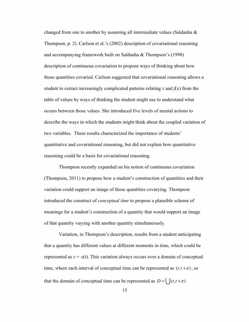
Thompson recently expanded on his notion of continuous covariation
(Thompson, 2011) to propose how a student’s construction of quantities and their
variation could support an image of those quantities covarying. Thompson
introduced the construct of conceptual time to propose a plausible scheme of
meanings for a student’s construction of a quantity that would support an image
of that quantity varying with another quantity simultaneously.
Variation, in Thompson’s description, results from a student anticipating
that a quantity has different values at different moments in time, which could be
represented as x = x(t). This variation always occurs over a domain of conceptual
time, where each interval of conceptual time can be represented as (t, t + ! ) , so
that the domain of conceptual time can be represented as D = (t, t + ! )!

16
(Thompson, 2011, p. 47). This characterization of variation allows the student to
anticipate that the domain of conceptual time is “covered” with these intervals, so
that, according to Thompson, the student can imagine that the quantity varies in
chunks of conceptual time while understanding that completed chunks can be
thought about as the quantity having varied continuously. At the same time, the
student can imagine the variation within chunks occurring in even smaller chunks.
Thus, a quantity varying over conceptual time can be represented as xe = x(te ) ,
where e represents intervals of conceptual time of size ! that the student imagines
becoming as small as possible.
Thompson’s characterization of variation extends to imagining two
quantities covarying, represented as (xe, ye ) = (x(te ), y(te )) , where (xe, ye )
represents an image of uniting two quantities, and then varying them in tandem
over intervals of conceptual time (Thompson, 2011, p. 48). This characterization
of covariation is similar to a function defined parametrically, which Thompson
alluded to in earlier work (Oehrtman, Carlson & Thompson, 2008). If a student
has this conception of covariation in mind, it is reasonable to assume they can can
think about (x(t), y(t)) = (t, f (t)) , which unites a function’s independent and
dependent quantity into an object. As that object varies over conceptual time, the
function is generated.
Saldanha & Thompson (1998), Thompson (2011), Carlson et al. (2002),
and Oehrtman, Carlson & Thompson’s (2008) work combines to support a
productive image for students thinking about function based on quantitative and
covariational reasoning. There is evidence that this approach can support a

17
student’s understanding of function in practice. These authors found that
covariational reasoning is productive for understanding function as a
representation of relationships in dynamic problem situations where multiple
quantities are varying simultaneously (Carlson et al., 2002; Carlson, Smith, &
Persson, 2003; Saldanha & Thompson, 1998; Thompson, 1994a, 1994b). They
found that understanding a function as an invariant relationship between
quantities, and imagining the values of those quantities varying simultaneously, is
critical to students developing a mature concept of function. They suggested that
thinking about functions using covariational reasoning allows students to interpret
tables, graphs, and algebraic formulas as various representations of a relationship
between two or more quantities. Thus, this dissertation drew on covariational
reasoning to support students’ development of function, but with explicit attention
to the students’ quantitative reasoning and use of conceptual time as a basis for
that covariational reasoning.
Quantitative Reasoning and Shape Thinking Given this study’s strong focus on graphs of functions, it was important to
focus on a construct I drew from my discussions with Patrick Thompson called
shape thinking. Shape thinking is an association the student makes with a
function’s graph. For example, a student might associate a function’s graph with a
particular shape with physical properties, while another student might associate a
function’s graph with a representation of quantities’ values. Thompson first
discussed the idea of shape thinking as he was creating case studies of an Algebra

18
I teacher in 2006, and I sought to expand on his characterization of shape thinking
by identifying and explaining understandings that were implicit in shape thinking.
Suppose a student associates a graph with a relationship between two
quantities’ values simultaneously represented on the coordinate axes. The
student’s attention to the axes suggests that he thinks about functions’ graphs as a
direct result of tracking the values of quantities on the axes. This student
associates the shape of the graph with a relationship between quantities, and the
graph is an emergent construction resulting from tracking and representing those
quantities’ values simultaneously. The association of a graph with an emergent
process was my initial conception of expert shape thinking.
Suppose a second student considers a graph as if a member of a class of
objects which he associates with a particular function definition. The student
might then accurately associate the graph with a type of function, but that
association would not entail a quantitative relationship. For example, many
students associate a graph that has a “U” shape with the function f (x) = x2 . In
this association, the student might think about the function’s graph as a wire that
could be manipulated without a transformation of the relationship between
quantities because in the student’s understanding, the graph is not associated with
quantities. The association of a graph with an object independent of any quantities
used to generate it constituted my initial conception of novice shape thinking.
Expert shape thinking relies on a student’s quantitative reasoning,
particularly when focusing on the quantities represented on the axes. I do not
claim novice shape thinking is bad, but I do not believe it is productive for
19
characterizing how a student might come to imagine a graph as an emergent
representation. Quantitative reasoning entails a way of thinking about situations
that is productive for students to construct and reason about functions, and was a
foundation for this study. If a student is to think about functions of two variables
as representing an invariant relationship among three or more quantities, then
identifying quantities, and constructing an image of their relationship to each
other is critical to defining and reasoning about the behavior of a two-variable
function.
Important Literature and Constructs This portion of the literature review synthesizes the literature relevant to
how students think about functions of two variables and their rates of change that
does not fall directly in the purview of quantitative and covariational reasoning. I
argue that understanding function is a difficult concept for students, and delineate
various frameworks for what it means to understand function. In doing so, I
discuss major results related to how students think about functions of one variable
to demonstrate how these results might be extended to functions of more than one
variable. Lastly, I propose constructs from literature about student thinking
relative to functions of one variable that are likely to be related to a students’
coherent conception of using two-variable functions and rate of change. In each
section, I focus on what work the literature does for this study, delineate what
work this study can do to contribute to what previous studies did not address, and
describe why I use quantitative and covariational reasoning in place of other well
known frameworks.

20
Students’ Difficulties in Developing a Mature Concept of Function
Researchers have found that it is difficult for students to achieve a concept
of function that the researchers would call mature, or advanced. Some researchers
refer to these students’ function concepts as incoherent. Often this incoherence is
in the researcher’s comparison of the student’s thinking to what we might call an
advanced concept of function while the student believes his understanding is
coherent. Carlson (1998) found that students receiving course grades of A in
calculus possessed an understanding of function that did not support the covariant,
or interdependent variance of aspects of the situation. Forty-three (43) percent of
the A students found f(x+a) by adding a on the end of the expression for f,
without referring to x+a as an input for the function (Carlson, 1998). Carlson et al.
(2002) found that students had difficulty forming images of a continuously
changing rate and could not represent or interpret inflection points of a function.
Oehrtman et al. (2008) suggested that students confused an algebraically defined
function and a formula, and proposed that many students believed all functions
should be tied to a single, algebraic formula.
Other researchers described students’ shortcomings in developing a
mature concept of function. Researchers described how the students referred to
functions as something that fits in set-correspondence diagrams and ordered pairs
(Akkoc & Tall, 2003, 2005), equated functions with a set of discrete instructions
for what to do with numbers (Bakar & Tall, 1992; Breidenbach et al., 1992),
thought about functions as equations (Dogan-Dunlap, 2007), and described

21
inconsistent images of a function across representations (Vinner, 1983, 1992;
Vinner & Dreyfus, 1989). Others suggested that students believed a function
behaves in a way that looked like the physical situation it was modeling
(Dubinsky & Harel, 1992; Monk, 1992a, 1992b; Monk & Nemirovsky, 1994),
saw little coherence between graphs, tables, and algebraic forms of the same
function (DeMarois, 1996, 1997; DeMarois & Tall, 1996), and had trouble
distinguishing between the behavior of the function and the behavior of the
function’s derivative (M. Asiala, Cottrill, Dubinsky, & Schwingendorf, 1997;
Habre & Abboud, 2006).
Many of these studies focused on the difficulties students had
understanding function, but in most cases their focus was on describing how the
students’ actions or descriptions differed from what the researchers would
consider an advanced concept of function, such as covariation or correspondence.
However, to characterize the difficulties a student has relative to function, one
must characterize his thinking to model the concept of function from the student’s
perspectives. My interpretation of these studies, based on their transcripts of
student talk, suggests that the root causes of these students’ shortcomings relative
to an advanced concept of function may be related to the students’ not
conceptualizing functions as invariant relationships between quantities. For
example, if a student thinks about the graph of a function as a number of points
connected by linear segments, it constrains the student from imagining that every
point on the graph of the function satisfies the invariant relationship between the
independent and dependent quantity.
22
In addition, it is not clear that researchers’ results extend to how students
work with functions of two variables because the tasks used in these studies did
not use functions, graphs, tables, or expressions that consisted of two variables.
For example, Akkoc & Tall (2003, 2005), Vinner & Dreyfuss (1989) and Vinner
(1989) posed tasks where students were asked to decide whether a particular
table, expression, or graph could be representations of a function. The tables
consisted of two variables x and y, the graphs consisted of points in the x-y plane,
and the expressions involved only one variable, x. Others studied how students
were able to find the output of a given function in graphical and tabular format
(DeMarois, 1996, 1997; DeMarois & Tall, 1996). The task they posed involved
tables where the columns were labeled x and f(x), and the graphs were in the two-
dimensional x-y plane. Finally, studies that asked students to generate a graph or
algebraic expression of a function given a physical model prompted students to
generate a function that related an input and an output quantity (Carlson et al.,
2002; Monk, 1992a, 1992b). For example, Carlson et al. (2002) posed the bottle
problem in which students were given a cross section of a bottle and asked to
generate a graph of the height of the water in the bottle as a function of the
volume of the water in the bottle.
I do not believe it is appropriate to draw conclusions from these studies
about how students think about two-variable functions because the tasks in these
studies did not include functions or situations with more than a single input and
output variable. My interpretation of the literature suggests to me that that
quantitative reasoning may be key in modeling the ways of thinking of students to

23
explain how these ways of thinking lead to the struggles documented by
researchers. However, research has not yet established that quantitative reasoning
is at the heart of students’ documented difficulties, and if it is, these studies’
results do not yet extend to student thinking about functions of two variables.
Characterizations of Understanding Function
This section considers the various descriptions researchers have made of
what it is entailed in understanding function, which I consider to mean the
development of a mature concept of function. I explain how these
characterizations of understanding function contributed to this study while also
focusing on the ways in which this study was different from previous
investigations. I show how thinking about functions as covariation of quantities
draws from several researcher’s perspectives, and how focusing on covariational
and quantitative reasoning support investigating a wide array of issues related to
students’ ways of thinking about function. It is also important to note that many
characterizations of understanding function treat understanding as if it is a
categorical, meaning a student has an a particular way of thinking or does not. I
have two issues with this approach. First, everyone has an understanding, or way
of thinking about function, which leads me to think about understanding as akin to
a continuous variable. Second, this way of thinking must be modeled and
compared to a “mature” model of function understanding. Thus, I interpret each
of these characterizations of understanding function as a model of an epistemic
student whose ways of thinking could be considered mature.
24
Multiple representations of function.
Several studies characterized students being proficient at generating, and
relating graphs, tables, and algebraic forms, and understanding those forms of
inscription can represent the same thing as an indication of a mature
understanding of function (Akkoc & Tall, 2003, 2005; Barnes, 1988; Bestgen,
1980; DeMarois, 1996; DeMarois & Tall, 1996). These researchers asked students
to complete tasks using graphs, tables, and analytic representations, and attributed
a student’s understanding of function to how well they were able to perform tasks
within these various milieus. They proposed that students understand function
after they have abstracted the commonalities among representations, which I
interpret to mean the student understands a table, graph and algebraic definition
are representations of a relationship between two or more quantities. For example,
Akkoc & Tall (2003), DeMarois (1996) and DeMarois & Tall (1996) suggested
that a student does not understand a function such as f(x) = 2x unless the student
thinks about the function in tabular and graphical form as equivalent to the
algebraic representation of the function. However, these studies did not explicitly
focus on what the students believed that graphs, tables, and algebraic forms
represented. This constraint did not allow the researchers to explain what it was
that students believed graphs and tables represented. This dissertation built upon,
and extended, these investigations by focusing on students’ thinking about the
extent to which graphs, tables, and algebraic forms could represent invariant
relationships between quantities.

25
APOS theory. Dubinsky & McDonald (2001) described APOS theory as a theoretical
framework that focuses on the processes an individual uses to deal with perceived
mathematical problem situations. APOS theory, in their description, arose from
the need to extend Piaget’s concept of reflecting abstraction to how students learn
mathematical ideas in collegiate mathematics. Asiala et al. (1996) modeled the
process by which an individual deals with a problem situation into mental actions,
processes, objects and schemas, which they referred to as, “APOS Theory”.
Asiala et al. (1996) defined an action as a transformation of objects
perceived as necessitating step by step instructions on how to perform an
operation. When an individual repeats, and reflects on an action, I interpret Asiala
to mean that the individual can create a process in which he can think about the
action without stimuli to necessitate the transformation. Asiala et al. described an
object as constructed by the individual reflecting on the process in a way that
allows him to think about the process as an entity on which transformations can
act. In Asiala’s description, a schema consists of the collection of actions,
processes and objects a student uses to think about a mathematical concept that
the student uses to deal with a perceived mathematical problem.
Dubinsky & Harel (1992) previously used these general descriptions of
action, process, object and schema to propose a framework for understanding
function. My interpretation of their work suggests that their framework serves as a
plausible model of a productive way of thinking about function. The model does
not require that all of these conceptions are necessary for a student to reason

26
coherently about function, but together, these constructs do form a descriptive and
explanatory model for a mature understanding of function. Dubinsky & Harel
(1992) described an action view of function in the following way:
An action conception of function would involve the ability to plug
numbers into an algebraic expression and calculate. It is a static
conception in that the subject will tend to think about it one step at a time.
A student whose function conception in limited to actions might be able to
form the composition of two functions, defined by algebraic expressions,
by replacing each occurrence of the variable in one expression by the other
expression and the simplifying; however, the students would probably be
unable to compose two functions that are defined by tables or graphs. (p.
85)
Students with an action conception of function can think about a function
as a specific rule or formula on which the student must imagine performing every
action. However, Dubinsky & Harel (1992) assumed the student is working with a
function defined symbolically. In their description of action, a student with an
action conception can only imagine a single value at a time as input or output, and
he conceives of a function as static, leading to seeing a function’s graph as a
geometric figure (Oehrtman et al., 2008). However, an action conception of
function that relies on quantitative reasoning can precede and does not necessitate
a symbolic representation of function. Instead, an action results from thinking of
two quantities varying in tandem, which does not require a symbolic
representation.

27
A student with an action conception of function, as defined by Dubinsky
and Harel, does not imagine the output exists until he has transformed the input.
This makes it impossible for the student to think about function as invariance
between an independent and dependent quantity because the output does not exist
until the input has undergone a transformation. However, a student with an action
conception of function who is using quantitative reasoning thinks of the output
and input existing simultaneously, which allows them to think about an invariant
relationship between those two quantities.
Dubinsky and Harel described a process conception as a more advanced
way of thinking about function:
A process conception of function involves a dynamic transformation of
quantities according to some repeatable means that, given the same
original quantity, will always produce the same transformed quantity. The
subject is able to think about the transformation as a complete activity
beginning with objects of some kind, doing something to these objects,
and obtaining new objects as a result of what was done. When the subject
has a process conception, he or she will be able, for example, to combine
it with other processes, or even reverse it. (p. 85)
Students come to have a process view of function once they have
repeatedly transformed an input to an output, and abstracted from those actions
that a function is a general input-output process. Once the student imagines
function as a process, a student can imagine the entire, dynamic input-output
process without having to perform each action. Students with a process

28
conception of function also conceive of functions as dynamic, where domain and
range are produced by “operating and reflecting on the set of all possible inputs
and outputs” (Oehrtman et al., 2008). Oehrtman et al. (2008) identified a process
understanding of function as critical to developing a coherent scheme of meanings
for function in calculus and more advanced mathematics.
According to Thompson (1994b), when a student possesses a process
conception of function and he can imagine the function as being “self-evaluating”
over a continuum of inputs, he may begin to think about a function as an object.
An object conception of function requires the student to think about function as an
object on which other functions can act. Thompson (1994b) stated that, “A
representation of the process is sufficient to support their reasoning about it, they
can begin to reason formally about functions – they can reason about functions as
if they were objects”. A student who thinks about function as an object is able to
think about a function as the input to a process and the results of that input
undergoing a transformation in the function. As the student solidifies a concept of
function as an object, he may begin to reason about operations not only on sets of
numbers, but sets of other functions. My study built on students thinking about
function as a process and object to inform the models I developed for student
thinking about two-variable functions.
Cognitive obstacles.
Sierpinska (1992) and Janvier (1998) proposed that a mature concept of
function results from one’s having overcome cognitive obstacles related to
understanding function, such as not being able to imagine numerous input and

29
output pairs (Janvier, 1998; Sierpinska, 1992), and the specific understandings
required in overcoming those cognitive obstacles. While they recognized that not
all learning is impasse driven, they constructed a plausible model for the
development of function based on impasses. Sierpinska (1992) and Janvier (1998)
reconstructed a possible process of learning a new idea, in this case function, as
best described by the qualitative jumps in understanding necessary to achieve an
“expert” way of thinking.
The cognitive obstacles that Sierpinska (1992) and Janvier (1998) focused
on were: identifying changes, discriminating between number and quantity, and
using functions as models of change in a situation. Their primary focus appeared
to be on students’ identification and representation of relationships between
changing quantities, which suggests that quantitative reasoning is critical to a
mature concept of function. In addition to the focus on quantitative reasoning,
Sierpinska (1992) and Janvier (1998) identified challenges students must
overcome in understanding function, but they did not say whether these
challenges remain the same as students start to think about two-variable functions.
While these challenges were not a direct focus of my study, I think that the type
of data I collected contributes to reconstructing their argument for two-variable
functions.
Characterization of Research on Multivariable Functions
Recently, several researchers studied how students solve problems
involving functions of two variables (Martinez-Planell & Trigueros, 2009;
Trigueros & Martinez-Planell, 2007, 2010), and another (Yerushalmy, 1997)

30
characterized how seventh graders could generalize ideas of one-variable
functions to two variables. Trigueros hoped to explicate students’ understandings
of functions of two variables (Martinez-Planell & Trigueros, 2009; Trigueros &
Martinez-Planell, 2007) by analyzing students’ responses to tasks focused on
identifying domain and range. Trigueros & Martinez-Planell (2007) suggested the
mental actions required to understand functions of two variables relied on
coordinating the Cartesian plane, real numbers, and an intuitive notion of three-
space. Building on their previous study, Trigueros and Martinez-Planell (2009;
2010) found that students had difficulty identifying the domain and range of
functions of two variables, and attributed this difficulty to a lack of coordination
of the schema for space and function. `
Yerushalmy (1997) described activities that she designed for seventh
graders that were intended to help them generalize their concepts of one-variable
functions to two-variable settings. She sought to gain insight into what
understanding students had formed about two-variable functions, and in what
manner those understandings had developed from understandings of one-variable
functions. She found that students’ representation of functions underwent major
changes that resulted in their creation of a new symbolic system for representing
two-variable functions. However, Yerushalmy did not clarify what the students
believed they had generalized as she did not focus on developing a model of the
student’s thinking based on her inferences in the course of the these interviews.
These investigations of students’ understanding of two-variable functions focused
on what students could or could not do (e.g. find the domain and range of a

31
function of two variables), rather than on their ways of thinking. Because these
studies were not focused on describing students’ ways of thinking, there is a
pressing need for investigations that focus on students’ ways of thinking about
function of two or more variables.
Students’ Thinking about Rate of Change
Students must attend to how quantities are changing with respect to one
another to represent dynamic situations with functions. Most calculus textbooks
present the idea of rate of change as a property that a function possesses.
However, rate of change can itself be thought of as a function whose values at an
instant tell you how fast one quantity is changing with respect to another at that
instant. Thus, a coherent understanding of rate of change of one quantity with
respect to another relies on thinking about function as covariation of quantities
and sustaining a process view of function.
Understanding rate of change is foundational to coherent ways of thinking
about major ideas in calculus (e.g. accumulation) and differential equations, yet
many students possess difficulties reasoning about rate of change (Carlson,
Larsen, & Jacobs, 2001; Carlson et al., 2003; Monk, 1987; Rasmussen, 2000;
Thompson & Silverman, 2008). Students’ difficulties understanding rate of
change range from problems interpreting the derivative on a graph (Asiala et al.,
1997), focusing on cosmetic features of a graph to talk about constant rate of
change of a linear graph (Ellis, 2009), assuming that a function and the rate of
change of a function must share specific features (Nemirovsky & Rubin, 1991a,

32
1991b), and displaying difficulties with activities designed to help them
understand the fundamental theorem of calculus (Thompson, 1994a).
Researchers have not only documented students’ difficulties
understanding rate of change, but have proposed ways of thinking and
understandings that explain their difficulties. Carlson et al. (2002) proposed a
covariational reasoning framework that centered on ideas of rate of change. Their
framework proposed mental actions (ways of thinking) and resulting behaviors
involved in a sophisticated understanding of covariation. The five levels of the
framework were (1) coordinating changes in one variable on changes in another
variable, (2) coordinating the direction of change of one variable with changes in
the other variable, (3) coordinating the amount of change of one variable with
changes in the other variable, (4) coordinating the average rate of change of the
function with uniform increments of change of the input variable and (5)
coordinating the instantaneous rate of change of the function with continuous
changes in the independent variable for the entire domain of the function.
Carlson et al. noted that the ability to move fluidly between mental actions
3, 4 and 5 was crucial to a student’s mature use of covariational reasoning. This
framework did not attribute a specific meaning to variable, but if one thinks about
variable as the representation of the result of measuring a quantity’s attribute, or
as the representation of a quantity’s magnitude, the mental actions rely on ideas of
quantitative reasoning, and thinking about function behavior using covariational
reasoning.

33
Thompson (1994a) proposed that the difficulties student’s displayed in
understanding the fundamental theorem of calculus arose from impoverished
concepts of rate of change and incoherent images of functional covariation. In that
paper, and others, Thompson constructed a hypothesized scheme of meanings and
ways of thinking that he believed were foundational to understanding rate of
change. Thompson described a rate as a reflectively abstracted constant ratio,
where a ratio is the result of comparing two quantities multiplicatively (p. 15).
Thompson & Thompson (1992) characterized the ways of thinking that support
understanding rate:
Between ratio and rate are a succession of images and operations.
We have identified, in principle, four levels in the development of
children’s ratio/rate schemes. The first level, ratio, is characterized
by children’s comparison of two taken-as-unchanging quantities
according to the criterion “as many times as”. The second level,
internalized ratio, is characterized by children’s construction of
quantities, where the accrual of the quantities occurs additively,
but there is no conceptual relationship between ratio of
accumulated quantities at iteration x and the ratio of accumulated
quantities at iteration x+i. The third level, interiorized ratio, is
characterized by children’s construction of covarying amounts of
quantities, where the amounts vary additively but with the
anticipation that the ratio of the accumulations does not change.
The fourth level, rate, is characterized by children’s conception of

34
constant ratio variation as being a single quantity – the
multiplicative variation of a pair of quantities as a measure of
single attribute (Thompson & Thompson, p. 8)
At the first two levels, the student only thinks in terms of static quantities.
Whether the student multiplicatively compares the quantities at iteration x only
(level one) or at iteration x and x+i (level two) and might find the quantities in the
same ratio, the student possesses no imagery of the quantities accruing in tandem,
and thus no relationship between the two ratios. At the third level, the student
imagines the quantities accruing simultaneously. At the fourth level, the student
no longer needs to focus on the image of two quantities varying in tandem, but
imagines the ratio of their measures as an attribute of the comparison of the
quantities.
Coinciding with level four, a general scheme for rate entails “coordinated
images of respective accumulations of accruals in relation to total accumulations.
The coordination is such that the student comes to possess a pre-understanding
that the fractional part of any accumulation of accruals of one quantity in relation
to its total accumulation is the same as the fraction part of its covariant’s
accumulation of accruals in relation to its total accumulation” (Thompson, 1994a,
p. 237). In others words, given that quantity A and quantity B covaried, if a/b’ths
of quantity A has elapsed, then a/b’ths of quantity B has elapsed. Building on a
general scheme for rate, Thompson described average rate of change of a quantity
as, “if a quantity were to grow in measure at a constant rate of change with
respect to a uniformly changing quantity, then we would end up with the same
35
amount of change in the dependent quantity as actually occurred” (Thompson,
1994a, p. 271). As a result, average rate of change relies on a concept of constant
rate of change, from which one constructs a concept of instantaneous rate of
change while understanding it cannot exist. Just as quantitative reasoning was
foundational to understanding functions, quantitative reasoning is critical to
students’ understanding rate of change.
Chapter Summary
In this chapter, I have reviewed the literature relevant to how students
think about functions of one and two variables. I have described quantitative and
covariatonal reasoning, and highlighted how past research findings provide a
basis for the design of this study. My synthesis of research relevant to this study
represents my thinking prior to carrying out the teaching experiments. The results
of this chapter also allowed me to develop a scheme of meanings I believed would
be productive for students’ understanding of two-variable functions and rate of
change. In the next chapter, I use the theoretical constructs from this review to
propose a scheme of meanings that constitute a mature understanding of two-
variable functions.
36
Chapter 3
CONCEPTUAL ANALYSIS
This chapter builds upon the constructs of quantitative reasoning,
covariational reasoning, and rate of change I described in chapter two. I propose
how relevant constructs can be extended to support students in thinking about
functions of two variables and their rates of change. I use the frameworks of
quantitative and covariational reasoning to explain a scheme of ways of thinking
that may comprise a mature understanding of functions of two variables and rate
of change. Thus, this chapter is extends the theoretical constructs from chapter
two to student thinking about two-variable functions and rate of change in space.
The ways of thinking I propose were not only targeted endpoints of my
instruction, they also described the ways in which students might need to reason
to achieve those endpoints. This mature understanding of two-variable functions
and rate of change in space was critical to the design of the study, including data
collection and analysis, which I discuss in the fourth chapter.
Conceptual Analysis
Thompson (2008) stated that conceptual analysis is useful in two ways.
First, one can generate models of thinking that aid in explaining observed
behaviors and actions of students. Second, one can construct ways of thinking
that, were a student to have them, might be useful for his or her development of a
coherent scheme of meanings that would constitute powerful understandings of a
mathematical idea. In the second type of conceptual analysis, the unit of analysis
is the epistemic student, which is a student assumed to have certain ways of

37
thinking about a mathematical idea. I used conceptual analysis to develop a
scheme of meanings and understandings based on quantitative and covariational
reasoning that I believed would comprise a mature understanding of two-variable
function in an epistemic student.
Critical Ways of Thinking: Functions of Two Variables
Whether we refer to function as static correspondence between sets or
function as a representation of systematic variation between two quantities, a
student must reason quantitatively about a situation in a way that allows him to
perceive of some regularity or rule governing the relationship between objects in
that situation. By reason quantitatively, I mean that the student perceives of a
situation in terms of relationships between quantities, which themselves are
composed of objects, attributes, and a perception by the student of that attribute as
measurable. Quantitative reasoning is also crucial to a student thinking about
function without an explicit context because the student can imagine that each
quantity in a situation has magnitude. By this, I mean the student recognizes that
the quantities have measures in some unit, but the quantities and units do not
really matter. What matters is that the student can focus on the magnitudes of the
quantity. By focusing on magnitude, the student is able to think about function as
a relationship between magnitudes, which allows him to think about functions
outside of a specified context.
Using an example mentioned earlier, a particle or piece of matter moving
through space does not possess “force”. A force is a result of an accelerating
mass, and mass times acceleration is a quantification of force. Mass, for example,

38
is the attribute of an object (such as a particle or piece of matter), which can be
thought of as an amount of stuff that does not vary under acceleration. If a student
is to construct an invariant relationship or correspondence it is important that he
imagine each quantity varying before imagining the simultaneous relationship
between the two quantities which forms their functional relationship. In the case
of a two-variable function, there must be at least three quantities, two of which the
student can relate by a quantitative operation, to form the third and whose values
can vary independently of each other.
The student must construct an image of the quantitative relationships
between two or more quantities varying individually, and then imagine that the
variation in two or more quantities occurs simultaneously to think about the
quantities as covarying. In this example, a change in mass and/or acceleration
produces a change in the force of a particle. The student must also imagine that
this relationship between force, mass, and acceleration can be measured. The
student must not only imagine that a relationship between quantities exists, but
also imagine that all quantities vary simultaneously, that mass and acceleration
can vary independently of each other, and that the relationship between values of
force and the values of mass and acceleration is invariant. It is important to note
that an invariant relationship need not be linear. The relationship between a side
of a square and the square’s area is invariant as the area is always the square of
the side length. Height as a function of age since birth is an invariant relationship
because I had a height at each moment, and my height at that moment will not
change.

39
The ways of thinking I have proposed support a student thinking about
function as a process. A student with a process view of function sees a function as
a generalized input-output process that maps a set of input values to a set of
output values, and is able to imagine running through a continuum of inputs as
well as the resulting outputs, as opposed to needing to plug individual numbers
into a formula. In the case of the three-variable example of force, a student
imagines a domain of values for mass and acceleration, but does not think about
only plugging in specific values to “find” the force. Instead, the student relies on
his knowledge of the invariant relationship to anticipate how force will vary in
tandem with acceleration and mass. In short, the student can imagine the entire
process of evaluating the function without having to perform each action (e.g.
plug in numbers for mass and acceleration to find force), and the process becomes
independent to where the student can focus on the relationship between quantities
expressed by the function without needing to consider the specific function to find
input and output. For example, a student may think about f(x) = 3x as a
relationship where the dependent quantity’s value is always three times as large as
the independent quantity’s value. The student can imagine a range of outputs that
are always three times as large as the corresponding inputs without needing to
plug each input into the formula. In this way, the student can think about
evaluating the function independently of the formula. I believe this is what
Thompson (1993) meant when he said that students reach a phase where they see
a function’s definition as having become “self-evaluating”—the student

40
anticipates without hesitation that providing the function an input immediately
results in an output that he anticipated would be three times as large.
A process view of function suggests a conception of a generalized input-
output process, but does not necessarily focus on how input and output vary in
tandem. For example, the student may understand that the output is three times as
large as the input, but may not be able to imagine the output and input varying
simultaneously. The student can build on thinking about function as a process to
think about function using covariational reasoning where a student holds in mind
an image of how the quantities’ measures vary in tandem (Saldanha & Thompson,
1998). Reasoning covariatonally involves thinking about how the value
represented by one variable changes with respect to a value represented by
another variable. To continue the accelerated particle example, one holds in mind
an image of force as a result of a quantitative combination of mass and
acceleration (notwithstanding arguments about the possibility of real-world
instantaneous speed) so that at every instant there is a force, mass, and
acceleration for a particle each of which is a quantity itself. Thus, covariational
reasoning about three variables, two of which are independent, rests on thinking
quantitatively about a situation.
A student must understand that function notation like F(t) = m(t)a(t) that
represents the invariant, co-varying relationship between one dependent and two
independent, coupled quantities that vary over conceptual time, while also being a
“rule” the student uses to calculate. Up to this point, I have not discussed function
in conjunction with a formula because in describing a coherent way of thinking

41
about two-variable functions, a formula does not really represent anything other
than an instruction to calculate until the student has achieved a process conception
of function. Achieving a process conception of function is non-trivial, and in the
next section I describe the ways of thinking that support a student forming a
process conception of sin(x).
Developing a Process Conception of Sin(x) Researchers (Moore, 2010; Thompson, 2008; Thompson, Carlson, &
Silverman, 2007) have demonstrated that developing a process conception of
sin(x) involves the following ways of thinking:
- Creating a meaning for x as measuring an angle’s openness. This entails
conceiving of the measure of openness as an arc measured in units of one radius
of any circle centered at the angle’s vertex.
- Locating the vertical displacement of the arc’s terminal point and conceiving of
the vertical displacement as measured in unit’s of that circle’s radius.
- Calling this vertical displacement measured in unit’s of the circle’s radius the
sine of the angle whose measure is x radii.
These ways of thinking then become a process that the student attributes to
the symbol sin(x). Given a process conception of function, the student can think
about a formula as representing a relationship between the vertical displacement
measured in units of the circle’s radius and the openness of the angle measured in
units of a circle’s radius. This provides the foundation on which the student can
imagine sin(x) (vertical displacement) and x as varying simultaneously where
sin(x) always depends on x. Next, I discuss how thinking about a function sin(x)

42
as covariation of quantities supports thinking about the construction of a
function’s graph.
Understanding a Graph of y = f(x).
Suppose that a student thinks about the graph of a function as constructed
by tracing out a point that simultaneously represents the values of two or more
covarying quantities. The following sequence describes a particular understanding
of a graph for y = f(x) and how that way of thinking extends to functions of two
variables. I use f(x) = sin(x) to illustrate what I mean by thinking about a function
as a tracing out of coupled quantities. Note that this part of the conceptual
analysis is based on ideas discussed by Pat Thompson within a functions course
for practicing teachers (http://pat-thompson.net/MTED2800/SchedFrames.html,
November 4).
! Imagine that there are two quantities in a situation, and that x and y
represent their respective values.
! Imagine that the x-axis represents all the possible values of a quantity’s
attribute measured in some unit.
! Imagine that the y-axis represents all the possible values of another
quantity’s attribute measured in some unit.
! Imagine the point that is y-units perpendicularly above the value of x
(represented on the x-axis). The coordinates of this point represent the
values of the two quantities simultaneously.
! Imagine a graph in two dimensions as the tracing out of that point which
simultaneously represents the value of x and y. (Figure 2)
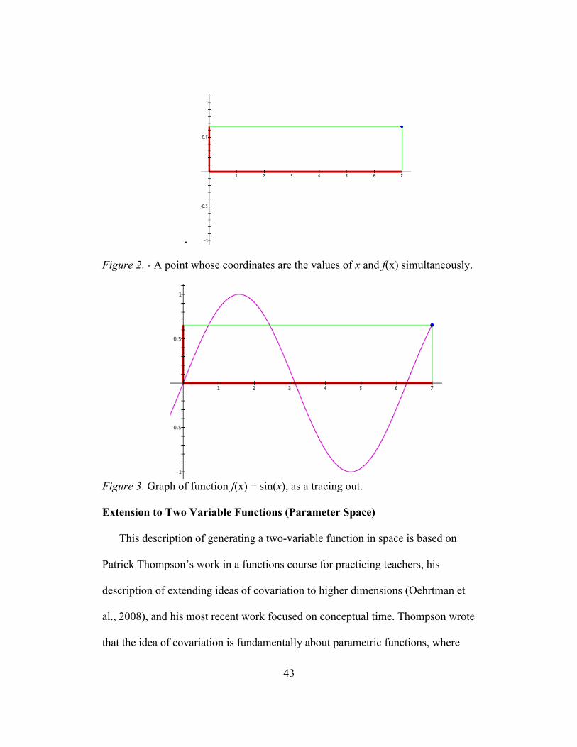
43
!
Figure 2. - A point whose coordinates are the values of x and f(x) simultaneously.
Figure 3. Graph of function f(x) = sin(x), as a tracing out. Extension to Two Variable Functions (Parameter Space)
This description of generating a two-variable function in space is based on
Patrick Thompson’s work in a functions course for practicing teachers, his
description of extending ideas of covariation to higher dimensions (Oehrtman et
al., 2008), and his most recent work focused on conceptual time. Thompson wrote
that the idea of covariation is fundamentally about parametric functions, where
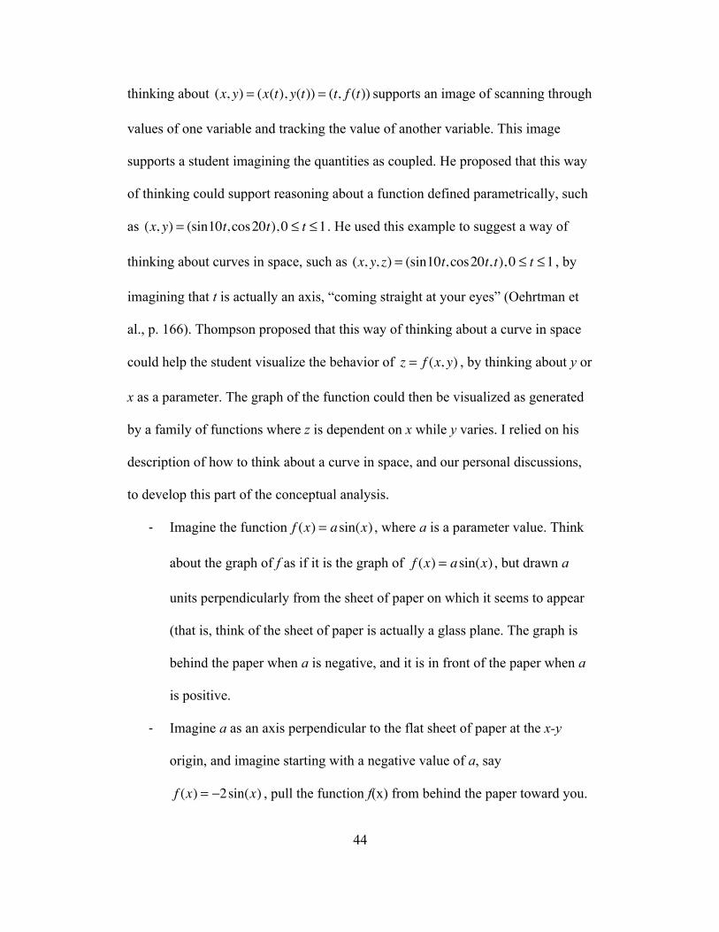
44
thinking about (x, y) = (x(t), y(t)) = (t, f (t)) supports an image of scanning through
values of one variable and tracking the value of another variable. This image
supports a student imagining the quantities as coupled. He proposed that this way
of thinking could support reasoning about a function defined parametrically, such
as (x, y) = (sin10t, cos20t), 0 ! t !1 . He used this example to suggest a way of
thinking about curves in space, such as (x, y, z) = (sin10t, cos20t, t), 0 ! t !1 , by
imagining that t is actually an axis, “coming straight at your eyes” (Oehrtman et
al., p. 166). Thompson proposed that this way of thinking about a curve in space
could help the student visualize the behavior of z = f (x, y) , by thinking about y or
x as a parameter. The graph of the function could then be visualized as generated
by a family of functions where z is dependent on x while y varies. I relied on his
description of how to think about a curve in space, and our personal discussions,
to develop this part of the conceptual analysis.
! Imagine the function f (x) = asin(x) , where a is a parameter value. Think
about the graph of f as if it is the graph of f (x) = asin(x) , but drawn a
units perpendicularly from the sheet of paper on which it seems to appear
(that is, think of the sheet of paper is actually a glass plane. The graph is
behind the paper when a is negative, and it is in front of the paper when a
is positive.
! Imagine a as an axis perpendicular to the flat sheet of paper at the x-y
origin, and imagine starting with a negative value of a, say
f (x) = !2sin(x) , pull the function f(x) from behind the paper toward you.

45
As you imagine pulling the graph toward you, imagine that the graph
adjusts for the changing value of a while also imagining its distance from
the x-y plane being a units behind or in front of it.
! Imagine that as you pull the function along the a axis, the graph of
f(x) = asin(x) has “fairy dust” on it, which creates a thin surface as the
graph of f is pulled along the a-axis. Each point on this surface has three
coordinates: x, a, and f(x).
The net effect of this collective of coordinated images and meanings is
that one sees a surface being generated as x varies to produce the graph of f for
a particular value of a while the value of a varies to sweep out a surface
generated by the family of graphs generated by x, f, and a.
Figure 4. Tracing out f(x,y) = ysin(x) in space.
Critical Ways of Thinking: Rate of Change in Space
Suppose that a student thinks about multivariable functions in the ways
described earlier in this chapter. That is to say, the student thinks about function
when reasoning about covariation of constructed quantities, when reasoning about
46
quantitative and numerical relationships, and specifically about properties of those
relationships (Thompson, 1994b). To think about rate of change in the context of
a two-variable function, a student must have a mature understanding of rate. To
imagine that a/b represents a value of quantity A measured in units of quantity B,
the student must think about the statement a/b=c as saying that a is composed of c
b-units. In this way, 16/5 = 3.2 says that 16 is composed of 3.2 units of five, or for
every five units of B, there are 3.2 units of A. Put yet another way, the student
understands that the statement 16/5 = 3.2 says that 16 is 3.2 times as large as 5.
Instantaneous and Average Rate of Change
To think about instantaneous rate of change as a limit of average rates of
change, the student must think about constant rate of change in the following way.
Suppose quantity A changes in tandem with quantity B. Quantity A changes at a
constant rate with respect to quantity B if, given any change in quantity B and the
corresponding change in quantity A, the changes in quantity A and quantity B are
in proportional correspondence. In other words, given that quantity A and
quantity B covaried, if a/b’ths of quantity A elapses, then a/b’ths of quantity B
also elapses . Thus, suppose that a function f changes from f(a) to f(b) as its
argument changes from a to b (Thompson, 1994a). The function’s output variable
(y) changes at a constant rate with respect to its input variable (x) if whenever
a/b’ths of b-a has elapsed, then a/b’ths of f(b)-f(a) has elapsed.
Though instantaneous rate of change exists mathematically, there is no
way to talk about instantaneous rate of change within a real world situation
without using approximations. Given that one thinks about rate as the constant

47
accumulation of one quantity in terms of the other, I suggest that for a student to
think about instantaneous rate of change, he must first understand that if a
function f changes from f(a) to f(b) as its argument changes from a to b, the
function's average rate of change over [a,b] is that constant rate of change at
which another function must change with respect to its input to produce the same
change f produces over the interval [a,b] (Figure 5, adapted from Patrick
Thompson’s functions course).
Figure 5. Average rate of change function as constant rate of change.
If a student thinks about average rate of change in this way, by attending
to the constant rate of change of covarying, accumulating quantities, then
instantaneous rate of change is “unreachable”. By unreachable, I mean the student
cannot viably say that at a specific instant, quantity A is changing at some exact
rate with respect to quantity B. Instead, this instantaneous rate of change is the
result of a finer and finer approximation, generated by considering average rate of
change of quantity A with respect to quantity B over smaller and smaller intervals
of change for quantity B. The formula for instantaneous rate of change,
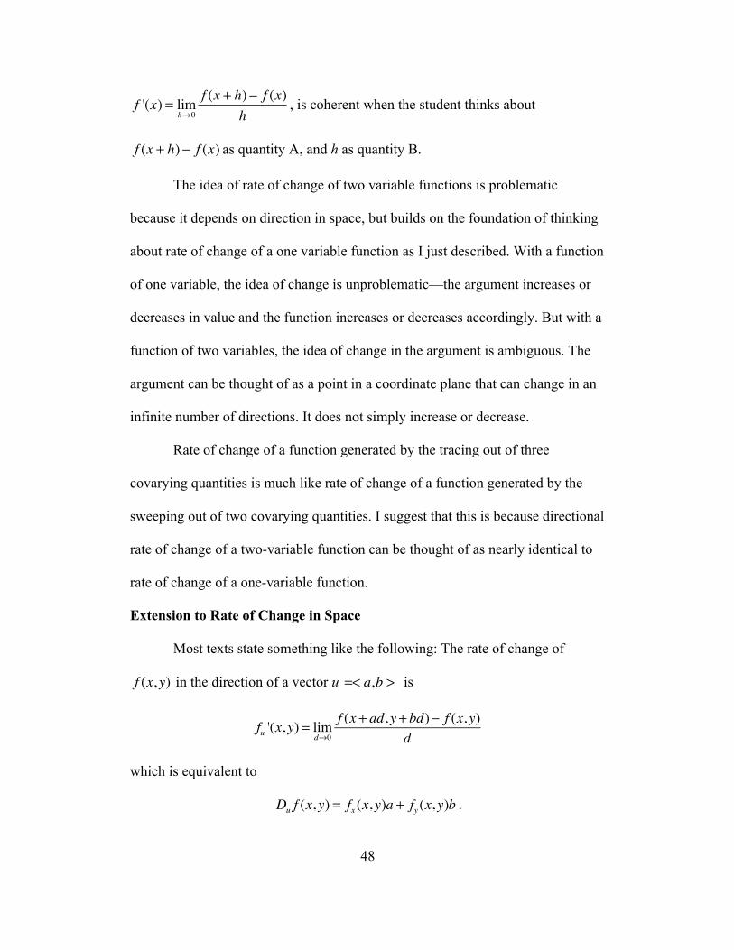
48
f '(x) = limh!0
f (x + h) " f (x)h
, is coherent when the student thinks about
f (x + h) ! f (x) as quantity A, and h as quantity B.
The idea of rate of change of two variable functions is problematic
because it depends on direction in space, but builds on the foundation of thinking
about rate of change of a one variable function as I just described. With a function
of one variable, the idea of change is unproblematic—the argument increases or
decreases in value and the function increases or decreases accordingly. But with a
function of two variables, the idea of change in the argument is ambiguous. The
argument can be thought of as a point in a coordinate plane that can change in an
infinite number of directions. It does not simply increase or decrease.
Rate of change of a function generated by the tracing out of three
covarying quantities is much like rate of change of a function generated by the
sweeping out of two covarying quantities. I suggest that this is because directional
rate of change of a two-variable function can be thought of as nearly identical to
rate of change of a one-variable function.
Extension to Rate of Change in Space
Most texts state something like the following: The rate of change of
f (x, y) in the direction of a vector u =< a,b > is
fu '(x, y) = limd!0f (x + ad, y + bd)" f (x, y)
d
which is equivalent to
Du f (x, y) = fx (x, y)a + fy (x, y)b .
49
It is important to keep in mind that <a, b> is a vector quantity and is the
sum of <a, 0> and <0, b>. Thus, the statement Du f (x, y) = fx (x, y)a + fy (x, y)b
says that the rate of change of the function f in the direction <a, b> is the vector
sum of its rates of change in the directions of its component vectors.
These textbooks refer to the instantaneous rate of change of the function f
at a fixed point (x0 , y0 ) , in the direction of u. This definition is problematic
because it assumes a student understands the necessity and use of a direction
vector. It is important that the student thinks about the rate of change of a function
as a change in its value relative to a change in its argument, and to understand this
in a way that aligns with the way he thinks about the rate of change of a single
variable function relative to its argument. To do this, one must imagine picking a
point P (x0 , y0 , z0 ) on the surface “at” which he wants to “find” the function’s rate
of change in a certain direction.
If a student is to understand rate of change of a two variable function using
similar meanings to a one variable function, she must consider what it means for a
quantity A to change at a constant rate with respect to quantities B and C.
Suppose that quantities A, B, and C covaried. Quantity A changed at a constant
rate with respect to quantities B and C if for any amount of quantity A elapsed
(a/b’ths), a/b’ths of quantity B elapsed, and a/b’ths of quantity C elapsed.
Extending this to function notation results from thinking about f (x, y) as quantity
A, and x and y as quantities B and C. This conception of rate of change
necessitates the idea of considering a direction of change, as there are an infinite
number of directions in which f(x,y) changes with respect to x and y. The

50
direction actually specifies the relationship between x and y. For example, the rate
of change of f(x,y) = 3x + 5y from a point (x0,y0) will be constant for any changes
in x and y only if !y is a linear function of !x.
Instantaneous rate of change can be thought of as an average rate of
change over an infinitesimal interval. The average rate of change of a quantity C (
f (x, y) ) with respect to quantities A (x) and quantity B (y) in a given direction in
space can be thought of as the constant rate at which another quantity D would
need to change with respect to quantities A and B to produce the same change as
quantity C in the same direction that (x,y) changed. This necessitates that quantity
D accrue in a constant proportional relationship with quantity A, and
simultaneously accrue in a constant proportional relationship with quantity B.
These understandings support thinking that as with functions of one variable, an
exact rate of change is a construction of an average rate of change between two
“points”. The points here are (x0,y0 , f (x0,y0 )) and (x1,y1, f (x1,y1)) .
Thus, the average rate of change between those two points is the constant
rate at which another function g(x, y) would need to change with respect to x and
y over the intervals [x0 , x1] and [y0 , y1] to produce the same net change as f (x, y)
over those same intervals. The function g(x, y) must change at a constant rate
with respect to x and a constant rate with respect to y and those constant rates
must remain in an invariant proportion, which necessitates x and y accruing in an
invariant proportion as well. An “exact” rate of change then, is a result of
considering an average rate of change of f (x, y)over an infinitesimally small

51
interval of [x0 , x1] and [y0 , y1] , where changes in x and y also covary in constant
proportion to each other.
The denominator for the rate of change of a two-variable function
f '(x, y) = limh,k!0
f (x + h, y + k)" f (x, y)?
does not initially make sense because it
seems as if h and k vary independently. Thinking about the rate of change of
f (x, y) as above supports thinking that any accrual d of either x and y must be
made in constant proportion b/a. This proportion a/b actually specifies the
direction vector to which many calculus books refer.
Thus, rate of change of f(x,y) with respect to x can be reformulated as
fu '(x, y) = limd!0f (x + h, y + k)" f (x, y)
d, where ad = h and bd = k so h must be
a/b’ths of k and k must be b/a’ths of h. Then, d can be thought of in the same way
as h in the one-variable case, where the student thinks about the derivative as an
average rate of change of a function over infinitesimal intervals while realizing
that the proportional correspondence between h and k means they have a linear
relationship resulting in approaching the point (x0,y0) along a line.
Directional Rate of Change and Path Independence
It is important to note that the conceptual analysis I have described above
does not immediately extend to a student thinking about rate of change in many
directions simultaneously. However, I believe it is necessary for a student to be
able to think about rate of change in at least one direction, which is a focus of this
conceptual analysis, if they are to be able to think about rate of change in all

52
directions. I conjectured that to think in all directions, they must think about a
single direction as a special case.
Suppose that a student has the ways of thinking I previously described
about rate of change in one direction in space. If he is to think about rate of
change in all possible directions, I believe the student must first consider when a
rate of change exists at a point in space. The student must understand that for
f '(x, y) to exist at a point in space, fu '(x, y)must be equivalent regardless of the
direction of the rate of change. This way of thinking provides the foundation for
the student to think about path independent rate of change. While path
independence was not a primary focus of this study, two students did make
progress in thinking about rate of change in all directions in space.
Chapter Summary The goal of this chapter was to use the theoretical constructs from
quantitative reasoning, covariation, and rate of change to establish a coherent
scheme of meanings that, were a student to have them, he or she would possess a
mature understanding of two-variable functions and a coherent understanding of
the concept of rate of change of a two-variable function with respect to its
argument. In establishing how I used theoretical constructs to establish specific
ways of thinking about functions of two-variables, I created the theoretical
foundation for the investigation. The conceptual analyses about two variable
functions and rate of change that I presented here drove the design, data
collection, and data interpretation for the study, all of which are the focus of the
next chapter.

53
Chapter 4
METHOD
This chapter describes the method I used to construct inferences about and
model student thinking during the course of and during analysis of the teaching
experiment sessions. First, I discuss the necessity of using a teaching experiment
given the constraints of the research questions I posed. I focus on the specific
elements of a teaching experiment and how they played a role in creating models
of students’ thinking about two-variable functions. Next, I explain the data
collection and interpretation procedures in the context of a teaching experiment
methodology. I then outline a set of tasks for the teaching experiment, and
describe how these tasks allowed me to generate and test hypotheses about
student thinking while also supporting students in developing the ways of
thinking described in the hypothetical learning trajectory in chapter three. These
foci allow me to describe how these tasks became didactic objects (Thompson,
2002) for me within the teaching experiment.
Rationale for a Using a Teaching Experiment
One cannot “see” a student’s thoughts as they exist in that student’s mind
without using one’s own scheme of meanings. For example, I could observe a
student using the words rate of change while calculating a derivative and assume
the student is thinking about derivative as measuring a change. This introduces
the first constraint in studying student thinking, that models of student thinking
are rooted in the observer’s schemes.

54
This constraint requires that the observer must show his interpretations are
viable. Viability in models of student thinking can be established by showing that
were students to think in ways the observer claims, their behavior would be
consistent with observed behavior. Chapter three was my attempt to establish the
viability of my schemes as producing worthwhile and achievable goals for
students’ thinking about functions of two variables.
Constructing a model that explains how students actually think about two-
variables functions required a methodology that allowed me to create a valid and
reliable model of student thinking. This study built upon Steffe and Thompson’s
(2000) account of a teaching experiment methodology that focuses on building
models of students’ ways of thinking about specific mathematical ideas and how
those ways of thinking develop in the context of instruction.
Steffe and Thompson (2000) proposed that the purpose of a teaching
experiment was to experience students’ mathematical learning and reasoning as a
first step to constructing models of students’ ways of thinking. They emphasized
that there are two realities at play within a teaching experiment. The first,
students’ mathematics, refers to the mathematical reality of the student, which is
unknowable to the researcher. Students’ mathematics is indicated by what they
say and do within a teaching experiment. The second, the mathematics of
students, refers to a researcher’s models of students’ mathematics, or ways of
thinking that, were a student to have them, would make the student’s actions and
utterances sensible for the student. Gaining insight into students’ mathematics is

55
critical for creating a viable model of how students understand and think about
functions of two-variables.
Given my goal of creating a viable model of students’ mathematics
relative to functions of two variables, a teaching experiment was most appropriate
for this study for three reasons. First, to propose models of students’ thinking that
might serve as desirable goals of instruction, I needed in some way to construct
and test the viability of the model’s “learnability” and potential difficulties
students might have in developing the ways of thinking that I have proposed.
Steffe and Thompson (2000) described a teaching experiment as an opportunity
for the researcher to experience constraints of language and actions of students,
which expands on the constructivist stance that our understanding of any reality
comes by way of experiencing the constraints it places on our actions. Second, a
teaching experiment breaks down traditional barriers between researcher and
teacher. Students are constantly constructing their own understandings, which I
gained insight into during a teaching experiment by using teaching to probe those
understandings. Third, a teaching experiment not only allowed for testing and
generating hypotheses at the beginning and end of the experiment, but gave me
opportunities to generate hypotheses about students’ ways of thinking continually
throughout the experiment.
Establishing the Viability of a Mathematics of Students The continuous cycle of task design and testing of hypotheses using new
tasks was the basis for establishing viable models of student thinking. By viable, I
mean models that provided descriptive and explanatory utility in a variety of

56
situations for a particular student. The continuous cycle of generating and testing
hypotheses allowed me to generate not only a possible model of how a student is
thinking, but one viable with the students’ actions and utterances during the
teaching experiment. Establishing a viable model of students’ mathematics was a
result of going through design and hypothesis testing in a way that allowed me to
experience the constraints on my actions due to students’ constraints on their
thinking that arose from their mathematics.
Steffe & Thompson (2000) identified two types of constraints in a
teaching experiment. First, I as the researcher experienced constraints in
understanding students’ mathematical thinking as a result of the utterances and
actions they brought forth in students. This was a necessary result of my own
schemes being different from those of the students. Second, students are
constrained by the their essential mistakes, which are mistakes created when the
demands of the task exceed the capability of their thinking. Essential mistakes
remain even in the face of instruction intended to help the student think in a
different way. Together, experiencing both types of constraints in the context of
generating and testing hypotheses about student understanding allowed me to
construct a model that addresses both the student’s capabilities and the student’s
limitations.
In the course of a teaching experiment, I attempted to make sense of
students’ thinking by hypothesizing ways of thinking that could plausibly lead to
the behavior that students exhibited. I tested these hypotheses within teaching
episodes by designing tasks and instruction that probed at the constraints
57
discussed above. For example, if I hypothesized that a student was thinking about
the graph of a function as a wire and not attending to quantitative relationships
that generated the function, I designed a task to elicit how a student was thinking
about transforming a graph, which I could model based on their actions and
responses to the task. If the student responded in a way that suggested he was
thinking about a graph as a wire, I designed a situation to create an essential
mistake if the student was in fact thinking about the graph as a wire. However,
during each teaching episode, it was critical that I put aside these hypotheses in an
attempt to influence students’ thinking positively while at the same time
respecting the thinking they have. It was after each teaching session that I
evaluated the hypothesis that led to the intervention and the revision of learning
goals.
If the hypotheses and the models of student thinking generated in an
episode were coherent with one another, I designed new tasks in which to test the
hypothesis again, but this time, if a hypothesized way of thinking seemed to make
a student’s actions coherent in a variety of situations, I claimed to have a viable
explanation of the mathematics of a student. If the hypotheses and the models of
student thinking generated in an episode were not coherent with each other, which
I defined as a deviation from the student behaving in the way I anticipated, I
developed new hypotheses and created situations in which to evaluate the
boundaries of students’ thinking. The ability to generate and test hypotheses while
experiencing constraints to model students’ mathematics relied on systematically
collecting data that allowed me to gain these insights.

58
Data Collection The following sections focus on my data collection and data interpretation
procedures to explain how I employed the theory of a teaching experiment to
investigate how students think about two-variable functions. In particular, I
describe how I used specific tasks to continuously generate and test hypotheses to
create models of students’ thinking, and use the hypotheses and reflections
generated from data collection to create an initial coding scheme for data
interpretation. Lastly, I describe my method for refining, and expanding the initial
coding scheme using open and axial coding (Strauss & Corbin, 1998) in tandem
with retrospective conceptual analyses.
Subjects, Setting and Logistics
Four students, Jesse, Jori, Brian and Neil participated in the teaching
experiments. Jesse and Jori participated in individual teaching experiments, while
Brian and Neil participated in a group teaching experiment. The four students
were in the process of taking a first semester calculus course that was grounded in
quantitative and covariational reasoning with an explicit focus on understanding
rate of change in the way I described in chapter three. I initially recruited six
students to protect against students dropping the course or becoming unavailable
to participate in the study and selected the students based on their willingness to
participate in the study, availability to participate at specific dates and times, and
their scoring at least an eight on the calculus concept assessment, which was
administered at the beginning of the semester.

59
Jesse was a conscientious student who expressed frustration that some of
his mathematics courses in high school had been focused on doing calculations
and learning algorithms without making sense of why the calculations and
processes were necessary or logical. He enjoyed mathematics because solving
problems was both fun and worthwhile. He was unsure of his future plans, but
was leaning toward majoring in mathematics and becoming an actuary in the
future.
Jori did not enjoy mathematics, which she attributed to numerous negative
experiences and perceived failure in high school mathematics and science
courses. She described herself as a high-achieving student “overall”, but felt
mathematics did not reflect her general success in other courses. She attributed
her success or failure to sources outside of her control, such as the teacher, the
workload of the class, or the general idea that mathematics is confusing.
Jori felt that doing mathematics involved memorizing procedures and examples
from the book or from the teacher’s presentations.
Neil was a computer science major, and described himself as passionate
about mathematics and science yet frustrated because he felt he was supposed to
remember so many formulas and methods instead of understanding why they
were true. He described his use of graphing calculators and technology as a way
to “remedy” the procedures he had forgotten. He felt that it was easy to unload the
calculations onto the technology, but was often unsure when it was a calculation
he was “offloading” as opposed to an important way of thinking. He described
himself as passionate about learning, and said his calculus course was something

60
he looked forward to because he was able to ask questions and debate others so he
could make sense of the rules and procedures.
Brian was a construction management major who had returned to school
that semester and chosen to take calculus because he was interested in
mathematics. He said that when he had an opportunity to make sense of ideas
instead of memorizing definitions, he found he loved “doing mathematics”, and
had purchased more advanced mathematics textbooks to read. Brian said he had
taken only basic mathematics in the past, but after a semester of work in calculus,
he described himself as excited to try new approaches in mathematics.
I met with each of these students during tutoring hours at least three times
in the weeks leading up to the teaching experiment. The tutoring hours were
specifically for the calculus one course in which the students were enrolled, and
the students asked questions related to course content and written homework
assignments. I asked all four students various questions related to their
understanding of function and rate of change, but the questions were not identical
as I related them to the homework questions the students brought to tutoring. I
also collected their in-class work and homework in the weeks prior to the teaching
experiment as background for my preparation. Meeting with the students and
observing their classroom participation and interactions prior to the teaching
experiment allowed me to become familiar with their particular approaches to
problem solving and their relationships with other students in the group, and it
allowed the students to become comfortable with me as a tutor.

61
The teaching experiments occurred over the last two months of the
calculus one course and the beginning of the summer session due to time
constraints in the student’s schedules. The first teaching experiment began after
the halfway point of the calculus course that allowed me to work with each
student and make initial hypotheses about their thinking with respect to rate of
change and graphs of one-variable functions. There were three teaching
experiments in total, two one on one teaching experiments and one group teaching
experiment involving two students and I. Each teaching experiment occurred over
a three-week period, or as the students’ schedules permitted. Table 2 provides the
meeting dates. Specific tasks and the day on which they took place were variable
across the teaching experiments. Thus, a detailed table with tasks and meeting
dates is available within each data chapter.
Table 2
Meeting Dates for Teaching Experiments.
Meeting Dates by Teaching Experiment
Jesse
(11 sessions)
(3/13/2011-4/4/2011)
Jori
(12 sessions)
( 4/5/2011-4/29/2011)
Brian and Neil
(9 sessions)
(5/5/2011-5/19/2011)
The students were compensated for their participation. Each teaching
episode occurred in a room with overheard cameras to tape both the students’
table and the classroom whiteboard. The students were able to use a laptop
computer, Graphing Calculator (a program installed on those computers), and had

62
table-sized whiteboards on which they were able to write anything they wished
during the sessions. Each session was videotaped on overhead and side view
cameras, the screen was recorded using SnapzPro, and the students’ written work
was recorded on a whiteboard and/or using the Livescribe Echo Smartpen.
Exploratory Teaching Interviews
The first step in creating a model of student’s mathematics was
constructing a set of initial hypotheses about their ways of thinking prior to the
teaching experiment, so that I was able attend to how these ways of thinking
persisted or changed in the course of the teaching experiment. To generate these
initial inferences, I used their tutoring hours to conduct exploratory teaching
interviews. It is critical to note that the exploratory teaching interviews were
based on problems the students were working on in tutoring, and thus, were not
always the same for each student.
Exploratory teaching interviews extend the clinical interview (J. Clement,
2000; Goldin, 2000) where one seeks to understand students’ thinking using task-
based questions, to include exploratory teaching where one attempts to help the
student extend their current ways of thinking to a desired understanding. These
interviews involved the student, an interviewer (me), and an interaction in relation
to questions, problems or activities (Clement, 2000, p. 519). The interviews
contained problems focused on revealing how students think about ideas of
quantity, variation, and function.
The interviews adhered to Goldin’s (2000) principles of structured
interviews (e.g. minimal heuristics, exploratory questions, choose accessible tasks

63
for subjects) while using the tasks as an opportunity to conduct exploratory
teaching about quantitative reasoning, covariation, and rate of change. For
example, I posed a bottle problem task, in which I ask the students to describe
what is happening to the height and volume of the water in the bottle as I pour an
equal amount of water into the bottle every second. I presented the task with
certain hypotheses about student thinking, such as the difficulty of thinking about
rates of change when the input unit is a generalized unit of volume. I asked the
student questions as he or she worked through and reflected on the task to gain
insight into his/her thinking, particularly focused on the student’s quantitative and
covariational reasoning. I used Goldin’s principles of structured interviews to
elicit language and actions of the student relative to the task, and to experience
students’ essential mistakes. During the interviews I continually attempted to
hypothesize about a student’s ways of thinking, and adjust the task, or ask
questions to create opportunities for students to reveal essential mistakes.
In the exploratory teaching interviews, I attempted to build on the working
model of a student’s mathematics to understand what progress the students made
given a certain instructional focus. For example, suppose that I established that a
student was thinking about creating a graph of height of the water in the bottle as
a function of volume of the water in the bottle by constructing a graph that fits the
shape of bottle in the problem. An important question was how resilient is the
student’s way of thinking—the extent to which it is resistant to instruction aimed
at changing it. Subsequent interactions moved progressively from probing
questions regarding what a point on the graph represented (indeed, even whether

64
the graph has points) to suggestions as to how she might try to think about where
graphs come from and what they represent about quantities in the situation.
In asking subsequent questions, I tried to establish whether the student was
thinking about a graph as connected to the shape of the given physical situation.
In the context of this study, I was interested in understanding what progress the
student can make by thinking about a graph as traced out by a point that
simultaneously represents the values of two quantities. Once I began to leverage a
model of the student’s mathematics to help move his/her thinking forward, I was
focused on exploratory teaching. In this case, I stepped back and helped the
student think about what it means to identify quantities, and how graphs are
representations of tracking how quantities vary in a given physical situation or in
abstract mathematical notation. I was especially attentive to the ease or difficulty
with which a student assimilated my suggestions during the exploratory teaching
episodes. If the student easily picked up the way of thinking I proposed, then this
suggested that their schemes were better formed than those of a student who
struggled to make sense of my suggestion. The nature of the student’s actions
subsequent to my suggestions often suggested their ways of thinking about the
ideas under discussion.
My goal in the exploratory teaching interviews was to make inferences
about each student’s thinking regarding quantitative reasoning, invariant
relationships among quantities, and functions of one variable and their graphs,
and to use those models to move the students forward in reasoning about
quantities, covariation and rate of change. While quantitative reasoning and rate

65
of change were foundational to the calculus course in which the students are
enrolled, I made no assumption that they were part of a student’s ways of
thinking. By establishing initial inferences about a student’s thinking, I was able
to adjust and refine tasks in the teaching experiment to allow me to experience
students’ essential mistakes firsthand. Essential mistakes are mistakes that help
the researcher define the boundaries of a model of a student’s way of thinking.
Teaching Experiment Sessions The teaching experiment sessions focused specifically on creating models
of student thinking, based on my inferences, while I attempted to help them think
in sophisticated ways about functions of two-variables and rate of change based
on the conceptual analysis in chapter three. The teaching experiment was based
on a set of tasks designed to gain insight into and foster ways of thinking of each
student by using exploratory teaching. It was productive not only to ask each
student what she was thinking, but to ask the students what sense they were
making of what other students are saying in the case of the group teaching
experiment, and of what I was saying in the case of the individual teaching
experiments. The specific tasks and content of the teaching experiment were fluid
because as I experienced specific constraints and generated and tested hypotheses,
I found it necessary to create new tasks or adjust the questions in a specific task to
establish the viability of a particular hypothesized way of thinking for a student or
the group of students. As the teaching experiment sessions occurred at least one
day apart, I was able to conduct initial reflections on what happened during each
episode, generate and test basic hypotheses, and adjust the next session based on

66
what occurred in the previous session. I recorded this process as text documents
before and after each teaching episode to generate data that allowed me to track
the development of my own thinking as a researcher.
Reflexivity: Documentation of My Thinking
It was critical that I accounted for my role in what the student said and did
and understand that my interpretations of student’s behavior and explanations
contribute to students’ actions, because my actions toward them were predicated
on my understandings of what they did. I emphasized earlier that a teaching
experiment breaks down the role of researcher and teacher. It also blurs the lines
between teacher and student because the student and teacher are co-constructors
of the teaching interactions. By this, I mean that both the researcher and the
student contribute ways of thinking, actions, and utterances that the other (student
or researcher) interprets and responds to in some manner.
Because I brought my own ways of thinking and specific interpretative
lens to the teaching experiment, I reflected on how students interpreted my
actions and how that interpretation might have played a role in the students’
actions. Sometimes, reflecting on one’s own actions is complicated, and
according to Steffe and Thompson (2000), an outside observer is one way to
enhance the researcher’s ability to reflect on his or her role in the interactions that
emerge. Due to time constraints and schedules of others, I was not able to have an
observer for most teaching experiment sessions. This required me to be diligent in
documenting the development of my own thinking within the teaching
experiment. In order to do this, I prepared a set of hypotheses about the student’s

67
actions prior to each teaching session, and my hypotheses were based on my
working model of their ways of thinking. Immediately after each teaching
experiment session, I watched the recording of the session, did a basic
transcription, and reflected on how the student’s actions within that session
necessitated adjustments or changes in my model of their thinking Thus, I was
able to simultaneously track my own thinking and the development of my model
for their thinking.
Teaching Experiment Tasks and Hypothetical Learning Trajectory The Homer Task
The initial tasks consisted of questions designed to reveal the meanings
each student attributed to the construction and interpretation of a graphical
representation of function. The task used the Homer activity (Figure 6), which is
an adaptation of Saldanha & Thompson’s (1998) City A – City B task. Trey Cox
and Scott Adamson changed City A to Shelbyville and City B to Springfield and
the car to Homer because in the Simpson’s episodes these cities move all around
the map episode to episode. In this version of the activity, built with Geometers
Sketchpad (Key Curriculum Press, 2010), Homer moves along a road with two
cities on either side. The cities’ locations can be manipulated, but their
representations, “Distance to Springfield” and “Distance to Shelbyville”, remain
as the vertical and horizontal segments, respectively. In the Homer adaptation, the
user could choose to have the animation reveal 1) Homer and the two cities, 2)
One or both segments, each of which represent Homer’s distance from Springfield
or Shelbyville, 3) A correspondence point which represents his distance from each

68
city simultaneously and 4) A graph created by tracking the correspondence point
as Homer’s distance from the cities as he moves back and forth on the road.
Figure 6. – Homer situation adapted from City A – City B (Saldanha &
Thompson, 1998).
Table 3
Task 1: Initial Questions for the Homer Animation. 1) Suppose the distance between this fixed point (a stationary object) and your right index finger, horizontal to the fixed point, represents Homer’s distance from Springfield. 2) Suppose the distance between this fixed point (a stationary object) and your left index finger, vertical to the fixed point, represents Homer’s distance from Shelbyville. 3) As Homer moves along the road, represent how Homer’s distance from Springfield is changing using your right index finger. With your left index finger, represent how Homer’s distance from Shelbyville is changing. 4) Next, place a finger in the plane so that its vertical distance from the horizontal axis represents Homer’s distance from Shelbyville and your finger’s horizontal

69
distance from the vertical axis represented Homer’s distance from Springfield simultaneously. Next, move your finger so that its position reflects Homer’s distance from each city as he moves along the road. 5) Finally, imagine that your finger that represents both distances has “paint” or “fairy dust” on it. Record what the paint would trace out as Homer moves along the road.
The goal of this activity was to gain insight into the extent to which
students were able to think about a graph generated by a sustained image of two
quantities varying simultaneously. This sustained image can be generated in the
following way. Suppose the student imagines Homer moving along the road over
an interval of conceptual time, and that the entire movement back and forth on the
road constitutes the domain of conceptual time over which his distance from each
city varies. If the student imagines each distance varying as Homer moves back
and forth on the road it is plausible the student can create an image of those
distances as coupled and varying in tandem over an interval of conceptual time,
represented by (xe, ye ) = (x(t), y(t)) . My intention was to support an image of a
graph as an emergent representation of tracking two quantities’ values. While the
graph in the Homer situation is a representation of a parametric function, I
anticipated it could be easily extended to thinking about a sustained image of x
and y covarying in the plane. Covariation in the plane, with y = f(x), would be
(x, y) = x(t), y(t)( ) = (t, f (t)) . However, the most important aspect of this task was
to think about a function’s graph as an emergent representation of two quantities
have covaried simultaneously. If the students initially had difficulty thinking
about a graph as generated by a sweeping out of a point that represented two
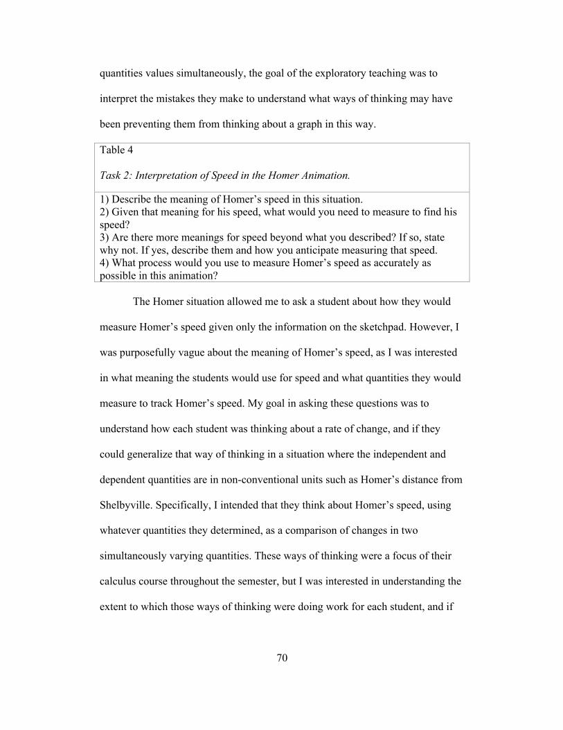
70
quantities values simultaneously, the goal of the exploratory teaching was to
interpret the mistakes they make to understand what ways of thinking may have
been preventing them from thinking about a graph in this way.
Table 4
Task 2: Interpretation of Speed in the Homer Animation. 1) Describe the meaning of Homer’s speed in this situation. 2) Given that meaning for his speed, what would you need to measure to find his speed? 3) Are there more meanings for speed beyond what you described? If so, state why not. If yes, describe them and how you anticipate measuring that speed. 4) What process would you use to measure Homer’s speed as accurately as possible in this animation?
The Homer situation allowed me to ask a student about how they would
measure Homer’s speed given only the information on the sketchpad. However, I
was purposefully vague about the meaning of Homer’s speed, as I was interested
in what meaning the students would use for speed and what quantities they would
measure to track Homer’s speed. My goal in asking these questions was to
understand how each student was thinking about a rate of change, and if they
could generalize that way of thinking in a situation where the independent and
dependent quantities are in non-conventional units such as Homer’s distance from
Shelbyville. Specifically, I intended that they think about Homer’s speed, using
whatever quantities they determined, as a comparison of changes in two
simultaneously varying quantities. These ways of thinking were a focus of their
calculus course throughout the semester, but I was interested in understanding the
extent to which those ways of thinking were doing work for each student, and if

71
little, to think about how to build on their current ways of thinking to reach a
working definition of rate of change.
Car A – Car B
The next task was the Car A- Car B problem (Hackworth, 1994, adapted
from Monk, 1992a), which displayed graphs of two cars’ speeds from zero to 1.2
minutes after they started from side-by-side positions. The problem depicted two
graphs, which the students were told represented the speed of each car (A and B)
as a function of time elapsed since the cars started traveling.
Table 5
Task 3: Interpretation of the Car A – Car B Graph. Two cars, Car A and Car B, started from the same point, at the same time, and traveled in the same directions. Their speeds increased, as shown in the graph (Heavy graph is for Car A, light graph is for Car B, so that after 1 minute they were both traveling at 100 mph. Was the distance between the cars increasing or decreasing after 0.8 minutes?
Figure 7. Car A - Car B from Hackworth (1994) adapted from Monk (1992a).
Hackworth (1994) found that the vast majority of college Calculus I
students (64 of 90) answered in a pretest before instruction on the derivative that
the distance between cars was decreasing because the graphs are getting closer
together. Interestingly, 42 out of 57 students (33 students had dropped) answered

72
on a posttest after completing study of the derivative that the distance between
cars was decreasing because the graphs were getting closer together.
I modified Hackworth’s protocol to first ask students where Car B was in
relation to Car A after 0.8 seconds had elapsed, and then asked them Hackworth’s
question. I used this task to gain insight into what they understood a graph to
represent, what they were paying attention to about a graph of a function, and
what information they would imagine using to construct the graph of a function.
The second focus of this task was to probe the students’ understanding of rate of
change, specifically comparing the rate of change of the two cars’ speed with
respect to time and the implication of a car’s speed relative to another as to what
is happening to the distance between them.
Table 6
Task 4: Interpretation of Rate of Change in Car A – Car B. Given the graph of Car A and Car B, describe what a rate of change of the quantities represented on the graph would represent. How would you measure the rate of change? Indicate this rate of change on the graph.
It was my intention to advance the students’ understanding of how they
would construct distance time and acceleration time graphs. Specifically, I wanted
to extend their ways of thinking to imagine creating the distance-time graph by
thinking about the speed-time graph as a rate of change function of the distance-
time graph. I also wanted each student to think about creating the acceleration-
time graph by thinking about the acceleration-time graph as a rate of change
function of the speed-time graph. In conducting the exploratory teaching
interview, I focused on having the students compare the similarities and
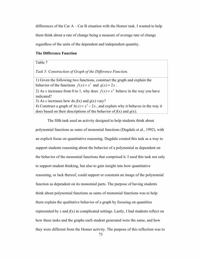
73
differences of the Car A – Car B situation with the Homer task. I wanted to help
them think about a rate of change being a measure of average rate of change
regardless of the units of the dependent and independent quantity.
The Difference Function
Table 7
Task 5: Construction of Graph of the Difference Function. 1) Given the following two functions, construct the graph and explain the behavior of the functions f (x) = x3 and g(x) = 2x . 2) As x increases from 0 to 1, why does f (x) = x3 behave in the way you have indicated? 3) As x increases how do f(x) and g(x) vary? 4) Construct a graph of h(x) = x3 ! 2x , and explain why it behaves in the way it does based on their descriptions of the behavior of f(x) and g(x).
The fifth task used an activity designed to help students think about
polynomial functions as sums of monomial functions (Dugdale et al., 1992), with
an explicit focus on quantitative reasoning. Dugdale created this task as a way to
support students reasoning about the behavior of a polynomial as dependent on
the behavior of the monomial functions that comprised it. I used this task not only
to support student thinking, but also to gain insight into how quantitative
reasoning, or lack thereof, could support or constrain an image of the polynomial
function as dependent on its monomial parts. The purpose of having students
think about polynomial functions as sums of monomial functions was to help
them explain the qualitative behavior of a graph by focusing on quantities
represented by x and f(x) in complicated settings. Lastly, I had students reflect on
how these tasks and the graphs each student generated were the same, and how
they were different from the Homer activity. The purpose of this reflection was to

74
understand whether students were able to think about the graphs in these tasks and
Homer situation as generated by keeping track of the values of coupled quantities
represented by a point.
The Box Problem The Box problem task, as I conceived of it for this study, was based on the
work of Marilyn Carlson’s Pathways to Calculus course. In the box problem, the
student must imagine making square cutouts from a rectangular piece of paper
and imagine folding up the sides to create an open box.
Table 8
Task 6: Construction of the Box. Suppose you are a computer programmer for a shipping company, and you are writing a program that will allow workers to print a shipping label that provides the volume of a box. The box is constructed from a rectangular piece of cardboard that is 33 by 24 inches, and is constructed by making cutouts from each corner of the cardboard. You need to construct a function so that when a worker inputs a cutout length, the function determines the resulting volume of the box and prints it on a shipping label.
Volume as a function of cutout length. The first part of the task required students to generate a function that
related the volume of the box to the length of the cutout. The question was
phrased so that students attended to the constraints of the cutouts to be made from
the box, particularly whether or not the cutouts need to be square and have equal
lengths. Previous interviews had indicated that constructing a function that
models volume as a function of cutout length required that the student construct
the box as a quantitative structure, that is, construct an image of the box how
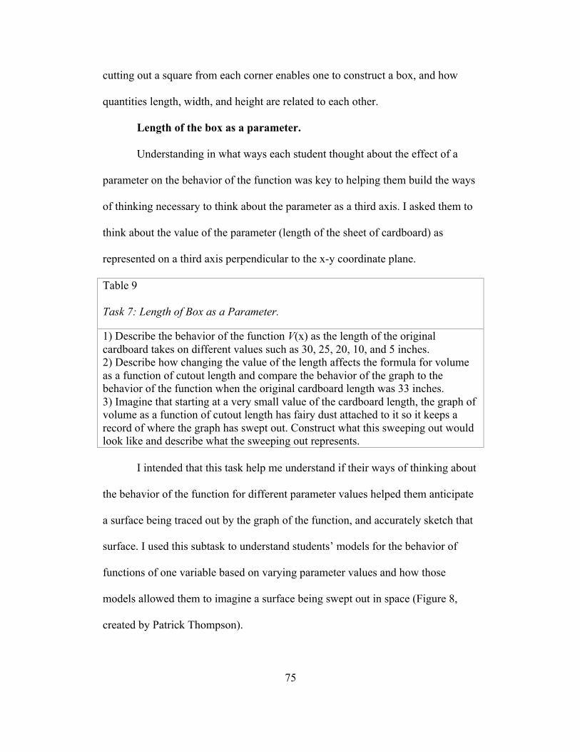
75
cutting out a square from each corner enables one to construct a box, and how
quantities length, width, and height are related to each other.
Length of the box as a parameter. Understanding in what ways each student thought about the effect of a
parameter on the behavior of the function was key to helping them build the ways
of thinking necessary to think about the parameter as a third axis. I asked them to
think about the value of the parameter (length of the sheet of cardboard) as
represented on a third axis perpendicular to the x-y coordinate plane.
Table 9
Task 7: Length of Box as a Parameter. 1) Describe the behavior of the function V(x) as the length of the original cardboard takes on different values such as 30, 25, 20, 10, and 5 inches. 2) Describe how changing the value of the length affects the formula for volume as a function of cutout length and compare the behavior of the graph to the behavior of the function when the original cardboard length was 33 inches. 3) Imagine that starting at a very small value of the cardboard length, the graph of volume as a function of cutout length has fairy dust attached to it so it keeps a record of where the graph has swept out. Construct what this sweeping out would look like and describe what the sweeping out represents. I intended that this task help me understand if their ways of thinking about
the behavior of the function for different parameter values helped them anticipate
a surface being traced out by the graph of the function, and accurately sketch that
surface. I used this subtask to understand students’ models for the behavior of
functions of one variable based on varying parameter values and how those
models allowed them to imagine a surface being swept out in space (Figure 8,
created by Patrick Thompson).

76
Figure 8. Sweeping out in the Box problem situation.
Length of the box as a variable. In part two, I focused on understanding students’ models for anticipating
the effect of a parameter on the behavior of the function. Part 3 focused on
helping students think about the parameter as a second variable, and having the
students discuss what it would mean to think about the length of the cardboard as
a variable instead of a parameter. Specifically, I used this task to gain insight
about how they represent the cardboard length as a variable instead of a
parameter, and to understand if the students used the same ways of thinking to
account for a as a variable as they accounted for it as a parameter.
Table 10
Task 8: Length of Box as a Variable. 1) Suppose you define a as variable. What does it mean to define a in this way? 2) What do you see as the difference between a parameter and variable in how you are using it in the Box problem? 3) What distinguishes a parameter and a variable, if anything, in your understanding?

77
At this point in the teaching experiment, I had students reflect on the
similarities and differences they saw in thinking about functions of one and two
variables. I provided specific questions asking them to compare the Homer
situation to the box problem situation, with particular attention to how they
thought about generating the graph of each function. I used these questions to
understand if the students were thinking about the graph in each situation as
generated by a tracing out of a point in the Homer task and then a two
dimensional graph in the box problem.
Rate of change of volume with respect to cutout length. In the last part of the task I asked students to focus on rate of change of
volume with respect to cutout length. I had them think about what the rate of
change of volume with respect to cutout length represents when volume is a
function only one variable, cutout length.
Table 11
Task 9: Rate of Change in the Box Problem. 1) Describe how the volume of the box changes with respect to the length of the cutout. 2) Construct a means to measure the rate of change, and interpret what a measurement of the rate of change means in this context. 3) Suppose the volume of the box is a function of two variables, base area of the box and cutout length of the box. Graph that function in Graphing Calculator. 4) Suppose we display a point on the surface of the graph. What does rate of change mean at that point? 5) How would you measure the rate of change at that point given the meaning you described?
Students had talked about rate of change extensively during their calculus
course, but I used this opportunity to understand what meanings the students

78
attributed to the phrase “rate of change”. I then focused on their meanings for rate
of change of volume with respect to cutout length where volume is now a function
of two variables, base area of the box and cutout length. I expected that the
students would puzzle over what it means to find a rate of change. When the
students constructed a graphical representation of the function in space, I
constructed a point on the graph, and asked them to interpret the meaning of rate
of change in the context of that graph at that point. I anticipated a key to this task
for students would be revisiting the definitions the students constructed for
constant, average, and instantaneous rate of change earlier in the teaching
experiment, and thinking about how those definitions fit with or did not fully
handle rate of change of a function of two variables.
I expected that students would immediately focus on the difficulty of
“calculating” the rate of change, so I asked them to think about how/if rate of
change has a different meaning in this context, and how one would represent that
rate of change. I used this task to gain insight into students’ models for rate of
change and how they imagined those models generalizing to account for a rate of
change of a function with two independent variables. I expected that it would be
key for me to discuss representing a rate of change given a specific relationship
between the two input quantities, much like indicating a direction vector for the
derivative. As a result of the exploratory teaching around this task, I intended the
students think about the rate of change of a function in space as representing the
rate of change in a specific direction in space. I intended that that this way of
thinking result from understanding that considering rate of change in a direction
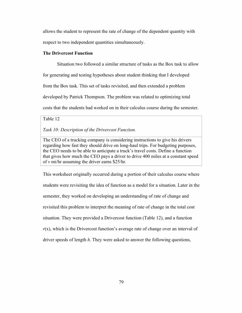
79
allows the student to represent the rate of change of the dependent quantity with
respect to two independent quantities simultaneously.
The Drivercost Function Situation two followed a similar structure of tasks as the Box task to allow
for generating and testing hypotheses about student thinking that I developed
from the Box task. This set of tasks revisited, and then extended a problem
developed by Patrick Thompson. The problem was related to optimizing total
costs that the students had worked on in their calculus course during the semester.
Table 12
Task 10: Description of the Drivercost Function. The CEO of a trucking company is considering instructions to give his drivers regarding how fast they should drive on long-haul trips. For budgeting purposes, the CEO needs to be able to anticipate a truck’s travel costs. Define a function that gives how much the CEO pays a driver to drive 400 miles at a constant speed of v mi/hr assuming the driver earns $25/hr. This worksheet originally occurred during a portion of their calculus course where
students were revisiting the idea of function as a model for a situation. Later in the
semester, they worked on developing an understanding of rate of change and
revisited this problem to interpret the meaning of rate of change in the total cost
situation. They were provided a Drivercost function (Table 12), and a function
r(x), which is the Drivercost function’s average rate of change over an interval of
driver speeds of length h. They were asked to answer the following questions,

80
1. Interpret r(x) = f (x + h)! f (x)h
(where h is fixed while x varies) in
terms of the situation being modeled, the meaning of the primary
function, and any value of h that you specify.
2. Give h a reasonable value for the situation being modeled.
3. Evaluate r(x) with several different inputs. Interpret each output in
relation to the input. Speak to trends and implications of what you
observe for the situation being modeled.
4. Graph y = r(x) at an appropriate scale. Interpret the graph. That is, say
what its point’s represent and information that you can get from the
graph.
Drivercost as a function of speed.
Table 13
Task 11: Parameterizing the Drivercost Function. 1) Construct a graph of the Drivercost function and anticipate the behavior of the graph of Drivercost function for Triplength parameter values 10, 100, 200, 400, 1000, and 5000. Do you anticipate any patterns in the behavior of the graph? 2) How is your thinking about this situation the same, and how is it different from thinking about length of the cardboard as a parameter in the Box problem?
The students had already determined in their homework that Drivercost is
a function of speed (v), where drivercost(v) = 25(400v) where 25 is the driver cost
per hour, and 400 is the trip length. I planned to have the students focus on how
changing the value of Triplength affects the formula for Drivercost as a function
of speed as well as the behavior of the graph as compared to the behavior of the
graph when the Triplength was fixed at 400 miles. By asking them to reflect on
81
the similarities and differences between the Drivercost function and the Box
problem, I hoped to elicit responses that would provide insight to their thinking
about how quantities’ values affect the behavior of a function.
Drivercost as a function of Triplength and speed.
This task built on part one by having students think about the Triplength
parameter as a second variable, and eliciting from students their ideas about how
considering Triplength as a variable was the same or different from thinking about
Triplength as a parameter. As with situation one, I used this subtask to understand
if the students used the same ways of thinking to account for Triplength as a
variable as they accounted for Triplength as a parameter. I also asked them to
reflect on how thinking about Triplength as a parameter or variable was the same
as or different from thinking about the length of the cardboard as a parameter or
variable.
Rate of change of Drivercost.
At the time of this study, the students had spent extensive time
constructing and thinking about the rate of change function in their calculus
course. In this situation, I asked the students to refer to the function Drivercost,
where drivercost(v) = 25(400 / v) , and answer questions one and four from their
previous worksheet. I anticipated that the students would have difficulty with
these questions even though they were focused on heavily in class. I anticipated
the difficulties would arise from a multitude of ways of thinking about the
meaning of rate of change, and I used this question to gain insight into students’
understanding of rate of change.

82
Table 14
Task 12: Rate of Change of Drivercost and Triplength. 1) Describe the meaning of the rate of change function in the driver cost situation, and describe how the graph of the rate of change function conveys that meaning. 2) Explore how changing the parameter values for Triplength affects the behavior of the rate of change function. What do you anticipate will happen? What do you notice about what happened, and did it fit with your conjectures? Why or why not? 3) Interpret the meaning of the rate of change function for the different parameter values of Triplength. Does the meaning change? I wanted to understand if thinking about the behavior of the rate of change
of the Drivercost function as they thought about the behavior of the Drivercost
function for parameter values of Triplength did work for how they thought about
rate of change. I attempted to gain insight into this question by asking the students
to interpret the meaning of the rate of change function for the different parameter
values of Triplength. In doing so, I wanted the students to consider how the
meaning of rate of change of Drivercost stayed the same or changed as Triplength
varied.
I wanted them to interpret the meaning of a point on the surface of this
rate of change function after they had constructed the graph of the function in
Graphing Calculator as a means to revisit the questions they answered in situation
one about the meaning of a rate of change of a function that represented a surface
in space.

83
Table 15
Task 13: Rate of Change of Drivercost as Two-Variable Function. 1) Using Graphing Calculator, graph Drivercost as a function of Triplength and speed. What does a point on the graph represent? 2) Identify a point on the graph of the function, and describe the meaning of rate of change at that point given the Drivercost context. 3) How would you measure the rate of change at this point? 4) Describe a more general process for measuring a rate of change at any point on the graph of the function? In this subtask, I built on part three by having the students imagine the rate
of change of Drivercost where Drivercost was a function of Triplength and speed.
I wanted the students to think about how various parameter values for Triplength
affected the behavior of the rate of change function for Drivercost, and used those
explorations to think about tracing out the rate of change of driver cost where
Triplength was now a variable. I anticipated that posing this question while
revisiting ideas discussed in the Box problem would allow me to gain insight into
the meaning they might make of rate of change of a two-variable function, as well
as the ways of thinking they use to develop a rate of change function for a given
function of two variables.
Specified Quantities to Using Variables Problems This task intended to engender student thinking about functions that did
not model a specified context. The reason for doing this was to understand how
the ways of thinking the students developed in the Box problem and Drivercost
function task could support or constrain them in their ability to reason about
functions of two variables without an underlying context to give the variables
meaning. I also anticipated using this situation to test hypotheses I developed

84
about the students’ ways of thinking in the Box problem and Drivercost function,
and that moving to a non-contextual situation would allow me to experience their
essential mistakes and further consider what sources might be leading to the
mistakes they made.
Behavior of t(x,a) = ah(x). Part one revisited the function h(x) from the pre-interview task based on
Dugdale et al.’s (1992) work. I asked the students, without first specifying
parameter values for a, to think about the behavior of the function t(x,a) = ah(x).1
I did not ask them to think about the behavior of the function ah(x) for parameter
values of a, as I wanted to see if thinking about t(x,a) as a sweeping out of h(x)
over a second variable a was a useful, or sensible way of thinking for the students.
Once they had constructed a graph and explained the behavior of the function
t(x,a), I asked each student to explain how they thought about generating the
graph, and if they thought about a in the same way as cardboard length and
Triplength in situations one and two. I anticipated that asking these questions
would allow me to understand if the students attributed common and coherent
ways of thinking through the three situations.
Rate of change of t(x,a) with respect to changes in a. In part two, I asked the students to determine a function that represented
the rate of change of t(x,a) with respect to changes in a and a function that
determined the rate of change of t(x,a) with respect to x. I did not pose
intermediary ways of thinking as I did in situations one and two as I hoped to
"#Other ways to symbolize what I called t(x, a) would be ta (x) or t(x, y) y=a .#

85
understand how the ways of thinking I focused on in the first two situations were
useful for the students given a situation without specified quantities. Once they
had generated a rate of change function for t(x,a) with respect to x or a, I asked
them to explain their reasoning, and to compare those ways of thinking to how
they approached the rate of change tasks in situations one and two. I anticipated
that by asking a question requiring reflection on all three situations, I could elicit
responses that revealed each student’s way of thinking about rate of change of
two-variable functions.
Post Teaching Experiment Interview Tasks The post-interview tasks were given the day after a teaching experiment
ended, and were structured as clinical interviews. I used these interviews as a way
to further test my hypotheses about how students were thinking about functions of
two variables and the rates of change of those functions. I designed the post-
experiment tasks toward the end of a teaching experiment, and constructed the
tasks to test the hypotheses I had developed after reflection on the teaching
experiment as a whole. For example, Jori’s post interview tasks were focused on
her reflection about her understanding of rate of change. Jesse’s focused on
thinking about graphical representation of three-variable functions because the
ways of thinking I believed the students reached in the teaching experiments were
different. In each teaching experiment, the tasks remained the same, but small
adjustments were made to the type of questions asked based on the previous
teaching experiments. I describe these adjustments in the data chapters.
86
Analytical Method: Conceptual and Retrospective Analyses
The data corpus consisted of video and audio of each interview and
teaching experiment session, recordings of my verbal and written reflections
before and after each teaching session, periodic reflections by the students
participating in the study, and written work of the students. This section focuses
on how I used the data to systematically construct models of each student’s
mathematics. The construction relies partly on systematic collection of data and
analytical procedures used to develop grounded theory (Strauss & Corbin, 1998).
The second use of conceptual analysis mentioned by Thompson (2008) is
to propose models of student thinking that help to make distinctions in students’
ways and means of operating, and to explain how these ways of and means of
operating persisted or changed during the teaching experiment. Retrospective
analysis consists of using the collected data to make a developmental analysis of
students’ mathematical constructions. This process involved viewing videotape
and reading reflections to recognize an interaction as already having been
experienced to make interpretations and hypotheses about students’ thinking that I
did not have in the moment of the teaching experiment. As I made interpretations
and hypotheses about my students’ understandings using retrospective analysis, I
used conceptual analysis to continually generate and revise a scheme of meanings
that would have made what the students said and did coherent for them. While
this conceptual analysis initially focused on observations I made during the
teaching experiment, the retrospective analysis allowed me to revise and expand
on the ways of thinking I attributed to each student during the teaching sessions.

87
Using retrospective and conceptual analysis required developing a systematic
coding scheme for the data. I used note-taking and basic transcription as a first
level of data analysis to generate a coding scheme for the entire data corpus.
The first level of analysis was note taking, which occurred between each
teaching experiment episode. I viewed all video and audio of the interviews and
teaching sessions and created a narrative of the students’ actions and responses
from the study. The second level of analysis consisted of taking observational,
methodological, and theoretical notes, which also occurred before and after each
teaching episode during the three teaching experiments. Observational notes
consisted of recordings like “this issue with graphing a function has happened
before”, “this way of drawing a graph might be important”, or “this way of
constructing a graph is something new for the student”. Methodological notes
consisted of observations about instructions given to the students, or issues that
were important to the methodology and conduct of the study. Examples are, “I
asked the question in a way that could have been confusing to the student”, or “I
assumed too readily that the student shared my understanding of the task. In
subsequent sessions, I was alert to the possibility that we did not possess the same
understanding.” Theoretical notes contained conjectures that explained students’
behavior and verbal descriptions. Examples are, “The student seems to be
thinking about a function as connected points, which would explain why she said
she needs to plot points to graph the function”, and “The student seems to be
thinking about the graph as a wire, which explains why he describes the graph
shrinking and expanding without reference to quantities.”

88
The note taking process and construction of a narrative facilitated my
abstraction of potential ways of thinking that the students exhibited over the
course of the teaching experiment. I documented these potential ways of thinking
and utterances to suggest ways of thinking that made these behaviors and
utterances sensible for the individual student. I looked for patterns in the
theoretical and observational notes, which led to the development of a coding
scheme for the video data.
I used StudioCode (Sportstec, 2009) to code videos and notes. The coding
process centered on theorizing about ways of thinking that explained categories of
student behavior by using a combination of open and axial coding (Strauss &
Corbin, 1998). Open coding consisted of a process by which I analyzed the data
collected in the interviews and teaching experiment sessions for instances of a
student verbalizing or constructing a concept identified from the note taking
process (e.g., graph of a function as a shape). Once I identified a major
phenomenon (e.g. graph of function as a shape or an object), I used axial coding
to identify the dimensions along which this category varies.
For example, one subject in my pilot study appeared to be thinking about a
graph as a “U” shape. Axial coding explicated the properties involved in thinking
about a graph as a shape. This involved systematically documenting what
indicated one was thinking about a graph as a shape, as opposed to other ways of
thinking. After identifying the major phenomena (e.g., graph as a shape; graph as
covariation of quantities), I coded video data to reflect instances of the interviews
and teaching sessions that reflect these phenomena. The coding of video data

89
served two purposes. It was a way to create objective counts of various coded
instances. But more importantly, the use of Studiocode to code video instances
allowed me to generate videos that contain all instances falling under a particular
code, which supported further conceptual analysis of ways of thinking that were
allied with the behavior that the code marks.
Coding of the video used the major phenomena generated from open and
axial coding to help me evaluate the usefulness of a particular explanatory or
descriptive construct. For example, in my pilot study, I initially generated
categories such as graph as covariation, graph as connected points, and graph as a
shape. After I used these constructs as code buttons, I found that what I had
referred to as graphs as connected points did not provide a great deal of
explanatory or descriptive power for explaining how a student thought about
graphing functions of one and two variables. If a particular construct did not do
enough work for generating models of student thinking, I reflected on how
thinking about the construct in a different way could provide more explanatory
power for the ways of thinking I elicited from students during the teaching
episodes.
Chapter Summary
This chapter explicated the method of collecting data and the theoretical
framework for interpreting it to create models of students’ mathematics. I
explained how I used the theoretical constructs of a teaching experiment to study
student thinking about functions of two-variables. I described a sequence of tasks
that help me to generate and test hypotheses about students’ understanding of

90
functions and rate of change. I suggested how this sequence of tasks could support
students developing a mature concept of two-variable functions as I outlined in
chapter three. Finally, I demonstrated how my data collection and analytical
method processes fit within the purview of my theoretical perspective, which I
hope demonstrates an epistemological coherence of this study.
91
Chapter 5
JESSE’S THINKING
This chapter describes how Jesse, a high-achieving student enrolled in
calculus one, thought about graphs of a function while viewing an animation of
independent and dependent quantities varying in tandem. Jesse was able to
imagine a point that swept out a graph of a one-variable function. He was also
able to imagine how the graph of a one-variable function swept out a graph of a
two-variable function. His attention to the axes seemed to allow him to think
about graphs as a representation of quantitative relationships.
In Part I, I show how Jesse was able to visualize graphs of two-variable
functions from various perspectives (z-x, z-y, y-x) by thinking about a variable as
a parameter and focusing on the relationship between the two quantities’ values
that were represented on the axes in that perspective. In this way, he was able to
anticipate, spatially, the behavior of a function from multiple perspectives and
reflect on how its three-dimensional representation was generated by the
relationships between quantities’ values. My inferences Jesse’s thinking suggest
that his visualization abilities allowed him to reason about how a surface was
generated, as well as to generate a three-variable graph from a two-variable
function defined algebraically.
Part II focuses on Jesse’s understanding of rate of change. His way of
thinking centered on the meaning of rate of change as a ratio of changes in two
quantities. He calculated the rate of change by using a measurement method

92
called the calculus triangle. The calculus triangle is a mnemonic for thinking
about measuring rate of change that Patrick Thompson has used for many years in
his courses and a teaching experiment in 2006 and was recently expanded upon to
characterize the images Thompson intended the calculus triangle to engender in
students (Weber, Tallman, Byerley, & Thompson, in press). The central issues
with which Jesse grappled were: (1) what it means for one quantity to change with
respect to two other quantities, (2) how to systematically “combine” rates of
change from each “perspective” in which he imagined using calculus triangles,
and (3) deciding what quantity’s change to make small. Jesse visualized
simultaneous calculus triangles in the z-x and z-y perspective, which involved
looking at a rate of change in a single direction by considering the x-y perspective
and treating z as a parameter value. This way of thinking prepared him to think
about a directional derivative by noticing that he could not add a “little bit” to
each independent quantity independently without generating an infinite number of
possibilities for the rate of change. Jesse believed it was necessary to add a little
bit to one quantity, which he conjectured would automatically add a little bit to
another quantity. His method required that he make only one change in a quantity
small—the other quantity became small because it was dependent on the first. As
a result, Jesse generated the rate of change functions for directional derivative and
partial derivatives, and reached a point where he was able to consider rate of
change in more than one direction.

93
Background
Jesse was high achieving in school, particularly in mathematics and
science. He attributed his past success to the teachers he had, to his desire to do
well in his courses, and his desire to understand the material so that he could teach
it to other students in his job as a high school mathematics tutor. Jesse said that he
generally understood the material well in all his courses and strove to make sense
of how ideas in a course fit together. He expressed frustration that some of his
mathematics courses in high school had been focused on doing calculations and
learning algorithms without making sense of why the calculations and algorithms
were necessary or logical. He enjoyed mathematics because he found solving
problems both fun and worthwhile. He often went above and beyond what the
class was doing to understand why things worked in both mathematics and
science.
Jesse was enrolled in first semester calculus while he participated in the
teaching experiment. I observed him in tutoring sessions throughout the semester
making sense of ideas like rate of change. He asked questions during class about
how mathematical concepts were related to other ideas from the course. When he
was not satisfied with his understanding, Jesse worked individually and with
tutors until he was satisfied.
Initial Inferences about Jesse’s Ways of Thinking I worked with Jesse ten times in tutoring sessions during the seven weeks
prior to the teaching experiment. His calculus instructor focused on quantitative

94
reasoning to support students’ thinking about functions and their rates of change.
During the three weeks prior to Jesse’s teaching experiment I began taking
detailed notes on our interactions during tutoring. I extracted a few general
observations from these notes, which became working assumptions I intended to
test systematically.
I noted that Jesse was attentive to describing relationships between
quantities in applied problem contexts. He defined an algebraic function or
created a graph to represent relationships between the quantities. Consistent with
the focus of the calculus course, Jesse attended to quantities in the problem, their
unit of measure, and on relationships between quantities’ values. Whether
working with an algebraically defined function or a function’s graphical
representation, he focused on describing how the input and output quantities were
related. For example, in describing the behavior of the function f(x) = 6x, he said
that the output is always six times as large as the input. I anticipated that these
ways of thinking would support him in making progress toward thinking about the
behavior of two-variable functions.
The teaching experiment with Jesse occurred over a period of three weeks.
The activities were based on the conceptual analysis and tasks presented in
chapters three and four. The table below shows the dates on which the activities
occurred. My interactions with Jesse centered around two themes: the behavior of
two-variable functions and how to think about how fast a two-variable function is

95
changing. These topics did not arise sequentially in the teaching experiment, but
for ease of description of my hypotheses, I present them separately.
Table 16
Task Sequence for Jesse’s Teaching Experiment.
Task Description Date (Day) Homer: Correspondence Points and Graphs 3/13/2011 (1) Homer: Discussing the Meaning of Speed 3/13/2011 (1)
Car A – Car B: Interpreting Meaning of the Graph 3/15/2011 (2) Car A – Car B: Measuring Rate of Change Using
the Graph 3/15/2011 (2)
Generating Graphs of f (x) = x3,g(x) = 2x 3/17/2011 (3)
Generating Graph of h(x) = x3 ! 2x 3/17/2011 (3)
Anticipating Behavior of m(x) = a(x3 ! 2x) 3/17/2011 (3)
Treating a as a Third Axis 3/17/2011 (3)
Box Problem: Box Construction and Treating Parameters as Variable
3/21/2011 (4) 3/23/2011 (5)
Box Problem: Interpreting the Meaning of Rate of Change at a Point in Space 3/23/2011 (5)
Box Problem: Measuring the Rate of Change at a Point in Space
3/23/2011 (5) 3/25/2011 (6)
Drivercost Problem: Parameters as Variables and Rate of Change 3/25/2011 (6)
Generalized Rate of Change Function and Direction
3/27/2011 (7) 3/29/2011 (8)
Generalized Functions: Construction and Interpretation of Graphs
4/1/2011 (9) 4/3/2011 (10)
Working with Strange Functions (More than 2 Variables) 4/4/2011 (11)

96
Part I: Jesse’s Ways of Thinking about Two-Variable Functions
Part I describes the sequence of tasks and development and testing of my
hypotheses about Jesse’s thinking about the behavior of two-variable functions.
Our discussions about behavior of two-variable functions and rate of change were
not sequential, but I present them as such to provide more clarity about the
development of my model for Jesse’s thinking. Table 16 outlines the days around
which I based the analyses and excerpts in Part I.
Day 1 – The Homer Activity
Based on my initial assessment of Jesse’s thinking during tutoring hours, I
predicted that, in the Homer situation, Jesse would construct Homer’s distance
from each of the cities as quantities and understand that as one distance varied the
other distance varied simultaneously. I also predicted, based on his approach to
thinking about graphs as generated by relationships between quantities, that
understanding a function’s graph as a sweeping out of a correspondence point
would fit with his understanding of representing a function’s behavior.
I introduced the Homer situation within Geometer’s Sketchpad (Figure 9),
and asked Jesse to explain what the diagram represented. He described how
Homer was traveling along a straight road and he imagined that there were
segments that measured Homer’s distance from Springfield and Shelbyville. I
asked Jesse to describe how he anticipated Homer’s distance from each city
would vary as Homer moved along the road to understand whether Jesse was
attending to the distances varying simultaneously.

97
Figure 9. The Homer situation in Geometer's Sketchpad. Excerpt 1 (Day 1 of TE, 00:00:25)
EW: As I animate Homer to move up and down the road, what will happen 1
to the two distances you mentioned? 2
Jesse: He, mmm, goes this way [demonstrates Homer moving from the top 3
end of the road to the bottom], and his distance from Springfield 4
increases and then decreases as I move the animation. 5
EW: What happens to his distance from Shelbyville as he moves? 6
Jesse: Well, his distance from Shelbyville also increases and then decreases 7
after he gets as close to Shelbyville as he can, which occurs when he is 8
perpendicular to Shelbyville from the road. I’m not sure exactly how 9
far he is from either of the cities, but one segment is longer than the 10
other. 11
EW: When he is travels over this segment of the road, what is happening to 12
his distance from Springfield? 13
Jesse: Well, when he is closest to one city, you can compare how close he is 14
to another city by the length of the other segment. Even though you 15

98
can’t measure it, you can compare the lengths of the segments to tell 16
which distance is greater. You sort of can always compare the 17
distances just by eyeballing it, so at anytime, I can tell which city he is 18
further away from.19
When I animated Homer to move along the road, Jesse pointed to the
screen as he described how Homer’s distance from Springfield varied (Excerpt 1,
lines 3-5). His description of Homer’s distance increasing and decreasing
precisely matched with the animation, and supported the idea that he was tracking
a distance. Jesse indicated that he was tracking Homer’s distance from a city
when he discussed minimizing Homer’s distance from Shelbyville (Excerpt 1,
lines 7-9). Subsequently, he described that while he could not say how far Homer
was from either of the cities exactly, he could imagine measuring those distances
using an ordinal comparison of the lengths of the segments he was imagining
(Excerpt 1, lines 9-11). This indicated to me he was thinking about these
distances as simultaneously varying quantities. Jesse made it clear that he was
imagining these quantities existing simultaneously when he said, “When he is
closest to one city, you can compare how close he is to another city by the length
of the other segment” (Excerpt 1, lines 14-15). His response suggested that he not
only imagined measuring the quantities ordinally, but that he could imagine
comparing the quantities’ magnitudes wherever Homer was located on the road.
I asked Jesse to track Homer’s distance from Shelbyville on the horizontal
axis, and Homer’s distance from Shelbyville on the vertical axis. I asked him to

99
predict the behavior of those segments as Homer moved on the road because I
believed that Jesse’s success at imagining the segments varying simultaneously
would indicate that he was thinking about the two distances’ magnitudes varying
simultaneously.
Excerpt 2 (Day 1 of TE, 00:00:36)
EW: As I animate Homer to move up and down the road, can you describe 1
how his distance from each city is varying and use the horizontal axis 2
for his distance from Shelbyville and vertical axis for Springfield? 3
Jesse: Sure, well, at the beginning [Homer at the top of the road] and he 4
begins, then his distance from both cities is decreasing, until he 5
reaches his minimum distance from, hmm, Shelbyville. After he gets 6
there, his distance from Shelbyville becomes larger, and his distance 7
from Springfield continues to get smaller, until he reaches his 8
minimum distance from Springfield, then he hits the end of the road, 9
turns around, and basically the opposite of what just occurred happens. 10
EW: It seemed when you were talking that you were concentrating really 11
hard on the screen, what were you focusing on? 12
Jesse: Well, it’s hard because as he is moving, both distances are always 13
changing so it is tough to track both of them on the axes at the same 14
time. It’s like if I forget one of them, it makes it easier, but it’s not 15
correct because I have to track both distances always. 16

100
Jesse’s response (Excerpt 2, lines 4-10) suggested he was thinking about
Homer’s distance from each of the cities varying in tandem (Excerpt 2, lines 4-
10). His language in lines 5-6, where he described the distance from both cities
decreasing, and line 8-9, where he described the distance from Shelbyville
increasing as the distance from Springfield decreasing, supported that he was
imagining the two quantities varying simultaneously. As he made those
descriptions, he said that both distances were always changing, and described the
necessity of tracking both distances always (Excerpt 2, lines 13-16). Jesse’s
description of each distance changing suggested he imagined them varying over
intervals of conceptual time. His described need for tracking both distances
simultaneously suggested to me that Jesse thought about the two distances
varying over the same intervals of conceptual time and had conceived of them as
covarying. It appeared that he had difficulty imagining how the quantities could
not be coupled, even as he struggled to verbalize their covariation.
In the following minutes, I asked Jesse to represent Homer’s distance from
Springfield using a vertical segment, extending upward from the point on the x-
axis that represented Homer’s distance from Shelbyville. This was the basis for
discussing the construction of the correspondence point that I introduced. The
correspondence point is the point whose coordinates correspond to the two
distances simultaneously. Jesse said that the correspondence point was created by
“programming”, where one “inputted” the distance from Shelbyville, which tells
the point “how far to move to the right of the origin”, and a distance from

101
Springfield, which tells the point “how far to move above the point which
represents Homer from Shelbyville”. I asked him whether it mattered in what
order the points were “programmed”. He noted that the correspondence point
needed to remain above the point that represented Homer’s distance from
Shelbyville, but in “reverse programming”, the point would “always be horizontal
to the point of Homer’s distance from Springfield”.
I anticipated, in the moment, that Jesse would visualize the behavior of the
point as dependent on two quantities’ values, Homer’s distance from Shelbyville
and Homer’s distance from Springfield. I believed this would support him in
thinking about the graph of a function as a tracing out of the “programmed”
correspondence point.
Excerpt 3 (Day 1 of TE, 00:01:09)
EW: So, if we imagine this correspondence point, can you tell me how it 1
behaves? [Correspondence point not displayed in GSP] 2
Jesse: Well, basically I just program the point so that it always represents the 3
two distances. It knows how far to be horizontally by distance to 4
Shelbyville and how far to be vertically by distance to Springfield. 5
EW: When I hit animate, I’d like you to imagine that the point [not shown 6
in GSP] leaves behind a trail, and to talk about how you think that trail 7
might appear. 8
Jesse: Well, it would leave behind a trail that sort of opens facing up, which 9
makes sense with my description about that representing programming 10

102
the two distances in at all times. The opening up and to the right comes 11
from both distances increasing at the same time. 12
EW: As we think about graphs, like a function f(x) = 2x, how is that the 13
same and different from this situation? 14
Jesse: Well basically the graph is made the same way. You program two 15
values in, 2x and x, and track the point as x changes, which is kind of 16
like making Homer move I guess. 17
Jesse’s description suggested to me he thought about the behavior of the
correspondence point as the result of programming the point to represent Homer’s
distance from each city (Excerpt 3, lines 3-5). I asked Jesse to imagine, without
actually seeing a correspondence point, that the point would leave behind a trail to
understand how he believed the correspondence point would behave. The trail he
anticipated was similar to that which the animation would produce if GSP actually
generated it (Figure 10).
!
Figure 10. Jesse’s anticipated trace of the correspondence point.
He described how the trail opened facing up (Excerpt 3, lines 11-12).
While Jesse was describing an opening up he was also attending to how the

103
correspondence point’s programming made the shape sensible by describing the
opening up as the result of both distances increasing simultaneously (Excerpt 3,
lines 11-13). I was convinced that he was able to think about a graph as generated
by a correspondence point, and that his idea of “programming” could extend
beyond the Homer situation. I asked him to compare the Homer situation to a
simple linear function (Excerpt 3, lines 16-17), and he described how he could
program the correspondence point using x and f(x) (Excerpt 3, lines 15-17).
Jesse’s responses suggested to me, in the moment, that he was thinking
about a graph of a function as generated by tracking and representing a
relationship between quantities (in the case of the Homer situation) and a
relationship between variables which represented the values of quantities (in the
case of f(x) = 2x). That he could imagine each situation entailing programming a
correspondence point made these two situations similar to Jesse. This suggested to
me that the correspondence point was a useful scheme for tracking quantities’
magnitudes simultaneously. I believed that his way of thinking about graphs prior
to this episode fit with thinking about a graph as a sweeping out of a
correspondence point. These episodes also suggested that Jesse’s attention to the
axes and his attention to which quantities’ values were represented on those axes
supported his anticipation of the behavior of functions and supported his ability to
reflect upon the graph he generated. His construction of a graph as an emergent
representation resulting from tracking quantities’ values supports this claim.

104
Following Day 1, I reflected about how Jesse was able to think about a
function’s graph as a sweeping out of a correspondence point. In this case, I
intended that Jesse think about the correspondence point representing two
functions of a single variable simultaneously, where each function represented
Homer’s distance from a city. Thus, Jesse appeared to be tracking (x(t), y(t)) , a
parametric function. I believed that this notion could be easily extended to
thinking about (x(t), y(t)) = (t, f (t)) in the one-variable function case. I
anticipated that in both cases Jesse would associate the graph as an emergent
construction dependent on how the correspondence point was “programmed”. I
anticipated that thinking about programming a correspondence point while
attending to the quantities’ values that were represented on each axis would
support him in describing the behavior of algebraically defined functions.
Day 3 – The Difference Function
Day 2 of the teaching experiment led to discussions about rate of change,
which I discuss in Part II. At the beginning of Day 3, I asked Jesse to anticipate,
through a verbal description of their covariation, the behavior of two functions,
f (x) = x3 and g(x) = 2x . Next, I asked him to represent this verbal covariation
using a graph. He explained that when he thought about a graph of a function, he
tried to recall the appearance of the graph in his graphing calculator. He explained
he could think about programming a correspondence point if the function was not
familiar to him. However, he said he would plot a bunch of points, and connect
them by making the intervals of change in the independent quantity very small.

105
Jesse explained that the graphs of f(x) and g(x) could be produced by
correspondence points that use (x, f(x)) and (x, g(x)) to “know how to behave”. He
described how those functions were relatively simple, but if they were more
complex, he would need to think about the behavior of the function using smaller
intervals of input to “understand what happens between the points that I decide to
plot”. He described how x and f(x) were similar to Homer’s distance from
Springfield and Shelbyville. In this excerpt, I asked him how he would think
about the behavior of a “difference of the two functions”.
Excerpt 4 (Day 3, 00:00:11)
EW: When you try to anticipate the behavior of the function f (x) = x3 ! 2x1
what do you pay attention to? 2
Jesse: Well, I know about programming the correspondence point, which is 3
still strange for me, but now I’m programming the difference between 4
two other correspondence points, x3 and 2x and the new point tracks x 5
and the difference between those two values [Creates Figure 11]. 6
EW: So what kind of graph do you anticipate would be produced? 7
Jesse: Let me think here [lengthy pause]. Well at first I thought it would be 8
like adding the two functions, but it’s the difference. I think it would 9
basically behave like x cubed the entire way because that term is much 10
bigger than 2x. [Graphs the function]. Wow, well, I was somewhat 11
right, but between here and here [-1 to 1 on the x-axis], it behaves 12
more like -2x. I guess when x is really small, oh wait! When x is less 13
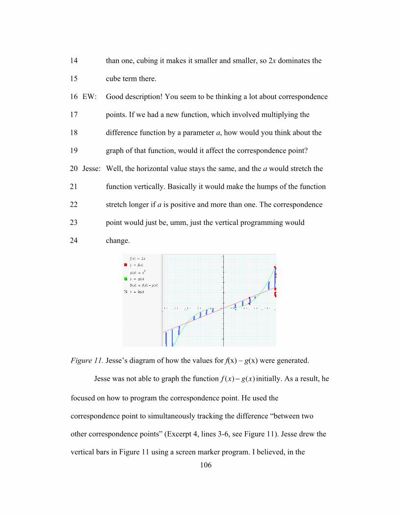
106
than one, cubing it makes it smaller and smaller, so 2x dominates the 14
cube term there. 15
EW: Good description! You seem to be thinking a lot about correspondence 16
points. If we had a new function, which involved multiplying the 17
difference function by a parameter a, how would you think about the 18
graph of that function, would it affect the correspondence point? 19
Jesse: Well, the horizontal value stays the same, and the a would stretch the 20
function vertically. Basically it would make the humps of the function 21
stretch longer if a is positive and more than one. The correspondence 22
point would just be, umm, just the vertical programming would 23
change.24
Figure 11. Jesse’s diagram of how the values for f(x) – g(x) were generated.
Jesse was not able to graph the function f (x)! g(x) initially. As a result, he
focused on how to program the correspondence point. He used the
correspondence point to simultaneously tracking the difference “between two
other correspondence points” (Excerpt 4, lines 3-6, see Figure 11). Jesse drew the
vertical bars in Figure 11 using a screen marker program. I believed, in the

107
moment, that Jesse was thinking about tracking the difference between two
functions because he said, “the new point tracks x and the difference between
those two values”, while simultaneously making the vertical bars in Figure 11.
Jesse appeared to think about a correspondence point as a general way to track
two quantities’ values. In this case, the length of the vertical bar represented one
value.
Jesse was initially confused about the function’s graph because the shape
he anticipated was not what he generated using Graphing Calculator (Excerpt 4,
lines 8-12). However, his attention to how the correspondence point was
programmed supported him in reasoning that the cubic term dominated the linear
term everywhere except in the interval [-1,1] (Excerpt 4, lines 12-15). Jesse then
thought about multiplying f (x)! g(x)by a parameter, and reasoned it would only
shift the correspondence point vertically. While he used the word “shift”, his
gestures indicated he was thinking about a “stretch” of the graph (Excerpt 4, lines
22-24).
My interpretation at that moment was that he programmed the
correspondence point with variables that represented unknown quantities’ values,
such as x and f(x). He used this same way of thinking to generate the graph for a
difference function f(x) – g(x), and anticipated the effect of multiplying the
difference function by a parameter by thinking about its effect on programming
the correspondence point. When Jesse was thinking about the behavior of a
function, he appeared to focus on understanding how to simultaneously represent

108
the covariation of two quantities’ values using coordinate axes. At the same time,
Jesse was not able to initially predict a graph of the difference function, which
indicated his programming scheme was limited by a focus on comparing the
numerical result of the cubic and linear term. His assumption that the cubic term
would always dominate the linear term constrained him from imagining that a
different relationship could be possible in the interval [-1,1] until he graphed the
function in Graphing Calculator. Thus, even though he could imagine
programming a correspondence point, his thinking limited him from a sustained
image of two quantities varying, which I believed could constrain him from using
the correspondence point as a scheme for generating graphs of functions.
Day 3 – Sweeping Out a One-Variable Function
During a ten minute break in the Day 3, I predicted that Jesse’s way of
thinking about a graph of a function as being generated by a correspondence point
would fit with thinking about a one-variable function in a plane generating a
surface in space. I planned to use his thinking about the parameter as representing
the distance in front of or behind the laptop screen to support a way of thinking
about a third axis along which a surface was swept out in space. After the break,
Jesse and I discussed thinking of a as a parameter that represented a distance in
front of or in back of the laptop screen on which the function h(x) = a(f(x) – g(x))
was displayed for a given value of a.
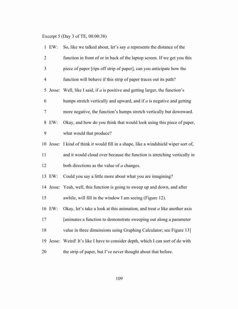
109
Excerpt 5 (Day 3 of TE, 00:00:38)
EW: So, like we talked about, let’s say a represents the distance of the 1
function in front of or in back of the laptop screen. If we get you this 2
piece of paper [rips off strip of paper], can you anticipate how the 3
function will behave if this strip of paper traces out its path? 4
Jesse: Well, like I said, if a is positive and getting larger, the function’s 5
humps stretch vertically and upward, and if a is negative and getting 6
more negative, the function’s humps stretch vertically but downward. 7
EW: Okay, and how do you think that would look using this piece of paper, 8
what would that produce? 9
Jesse: I kind of think it would fill in a shape, like a windshield wiper sort of, 10
and it would cloud over because the function is stretching vertically in 11
both directions as the value of a changes. 12
EW: Could you say a little more about what you are imagining? 13
Jesse: Yeah, well, this function is going to sweep up and down, and after 14
awhile, will fill in the window I am seeing (Figure 12). 15
EW: Okay, let’s take a look at this animation, and treat a like another axis 16
[animates a function to demonstrate sweeping out along a parameter 17
value in three dimensions using Graphing Calculator; see Figure 13] 18
Jesse: Weird! It’s like I have to consider depth, which I can sort of do with 19
the strip of paper, but I’ve never thought about that before. 20

110
Jesse’s windshield wiper metaphor (Figure 12), which he described as
“filling in” the window, suggested he was thinking about the family of graphs
moving within the x-y plane instead of thinking of it as a graph in space (Excerpt
5, lines 10-12). I suspected, in the moment, that Jesse had difficulty imagining a
single variable function sweeping out along a third axis because he believed a
sweeping out occurs within the plane. Given this assumption, I displayed an
animation of f (x) = sin(ax) as the value of a varied, without displaying its
definition, to demonstrate the type of visualization I intended to support (Figure
13). As he watched the animation, Jesse found it strange that he had to “consider
depth” (Excerpt 5, lines 19-20).
Figure 12. Jesse’s windshield wiper effect of the parameter a.
Figure 13. Using Graphing Calculator to support thinking with depth.

111
Jesse went on to say that thinking with depth was strange because he had
never thought about a graph in space. He noted that using depth created new ways
to look at functions represented in space because they could be viewed from
multiple perspectives. In Excerpt 6, he described his meaning for thinking with
depth and defined his meaning for “perspective”.
Excerpt 6 (Day 3 of TE, 00:01:05)
EW: We’ve talked a little about thinking with depth and it being important 1
for thinking about how to generate the surfaces in space. 2
Jesse: Yeah, well, at first it was weird for me to think about that, but after I 3
figured out what I needed to do, like treat something as a parameter, it 4
wasn’t that hard. So with our first function, I treated the parameter like 5
the extending axis. It’s kind of like you do two correspondence things, 6
one is the point that makes the 2-D graph, the other is the graph as the 7
correspondence thing, making the 3-D graph. 8
EW: You mentioned also you had another way of making the same 3-D 9
surface, how? 10
Jesse: Well, I was looking at some things, and if we call the output z [term 11
introduced by Jesse], we kind of created the z-x view before, where a 12
was like the y-variable. We could look at the z-y view too, where x is 13
the parameter and y is the variable. This would be like a z-y view. You 14
can kind of look at 3-D things from a lot of ways, you can just change 15
what you are calling a variable and what you are calling a parameter. 16

112
EW: That’s really interesting. So could you apply this to our original 17
function? 18
Jesse: Yeah, just make x3 ! 2x the parameter and a into the y-variable. Then 19
you will just have a linear function from the z-y view that moves to 20
create the same surface. I know the function will give me, umm, the 21
same surface, because in the z-x and z-y, I eventually treat both x and y 22
as a variable in both views, but just make that view easier to think 23
about by making one of them a parameter. 24
EW: So, in your mind, what’s the difference between a variable and a 25
parameter? 26
Jesse: A variable, you just let it represent all the values, but the parameter is a 27
snapshot of values of the variable, like in class, which you can control.28
Jesse’s responses suggested to me, in the moment, that he noticed a
similarity between sweeping out a point and sweeping out a function by sliding a
plane through space. In the first case, a point swept out to generate the graph of a
one-variable function, and in the second case, the graph of that one-variable
function swept out along a third axis to generate the graph of a two-variable
function (Excerpt 6, lines 3-8). The ease with which he designed a way to relate
one and two variable functions’ graphs being created suggested that he imagined
them as created by a “generating object”. The generating object for one-variable
functions’ graphs was a point and the generating object for a two-variable
function was the graph of a function in a plane, where the plane is determined by
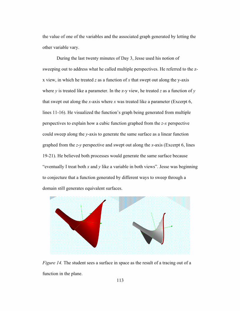
113
the value of one of the variables and the associated graph generated by letting the
other variable vary.
During the last twenty minutes of Day 3, Jesse used his notion of
sweeping out to address what he called multiple perspectives. He referred to the z-
x view, in which he treated z as a function of x that swept out along the y-axis
where y is treated like a parameter. In the z-y view, he treated z as a function of y
that swept out along the x-axis where x was treated like a parameter (Excerpt 6,
lines 11-16). He visualized the function’s graph being generated from multiple
perspectives to explain how a cubic function graphed from the z-x perspective
could sweep along the y-axis to generate the same surface as a linear function
graphed from the z-y perspective and swept out along the x-axis (Excerpt 6, lines
19-21). He believed both processes would generate the same surface because
“eventually I treat both x and y like a variable in both views”. Jesse was beginning
to conjecture that a function generated by different ways to sweep through a
domain still generates equivalent surfaces.
Figure 14. The student sees a surface in space as the result of a tracing out of a
function in the plane.
114
My reflections on Day 3 indicated Jesse’s way of thinking about
generating a one-variable function’s graph using a generating point supported him
in thinking about generating a two-variable function’s graph using a generating
graph of a function in the plane (Figure 14). I had not anticipated his initial
thinking that the family of graphs stayed in the x-y plane. However, I noticed that
his method of sweeping a curve through space as he varied the value of one of the
variables constituted a kind of “advanced shape thinking”. I conjectured that his
advanced shape thinking allowed him to imagine the function’s graph was
generated from a sweeping out along a third axis as a trail of the function’s values
restricted to a certain domain.
Days 4 and 5: The Box Problem
Days 4 and 5 were short sessions. I used them to evaluate my working
hypotheses about Jesse’s shape thinking and his use of perspectives. I anticipated
that in the box problem he would continue thinking about functions’ graphs from
multiple perspectives. I also believed he would need to relate the quantities in the
box problem using a functional relationship to imagine generating a surface in
space.
Excerpt 7 (Day 4 of TE, 00:00:06)
EW: Suppose you are a box designer, and you must program a computer to 1
determine the volume of an open box, which has no top to it. This 2
open box is created from making cutouts from a rectangular sheet of 3
115
paper. Jesse, could you tell me how you would think about making 4
such a box, as well as how to represent the volume of the box? 5
Jesse: Well, first, the formula is just length times width times height. So I 6
would need to make the cutouts, I’ll call the cutout the long way e 7
[motions along the longer side of the sheet of paper] and the short way 8
f [motions along the shorter side of the sheet of paper]. From what I 9
am imagining, I would subtract the e from the length two times and the 10
f from the width two times, and maybe the height of the box is half of 11
e times f? 12
EW: Say a little more if you can. 13
Jesse: Well, somehow the cutouts have to make the height of the box. Wait! I 14
guess e and f always need to be the same or the box would not be a 15
real box, at least not like the problem wants it to be. The height would 16
not be the same all around otherwise. 17
EW: How would you determine the height of the box? 18
Jesse: Well, by imagining folding up the box, it [pointing at the height on his 19
diagram] would have to be the same as e and f because they are the 20
same now. So the formula would be (l ! 2e)(w ! 2e)(e)where e is my 21
cutout. 22
EW: Formula for what? 23
Jesse: Volume of the box.24
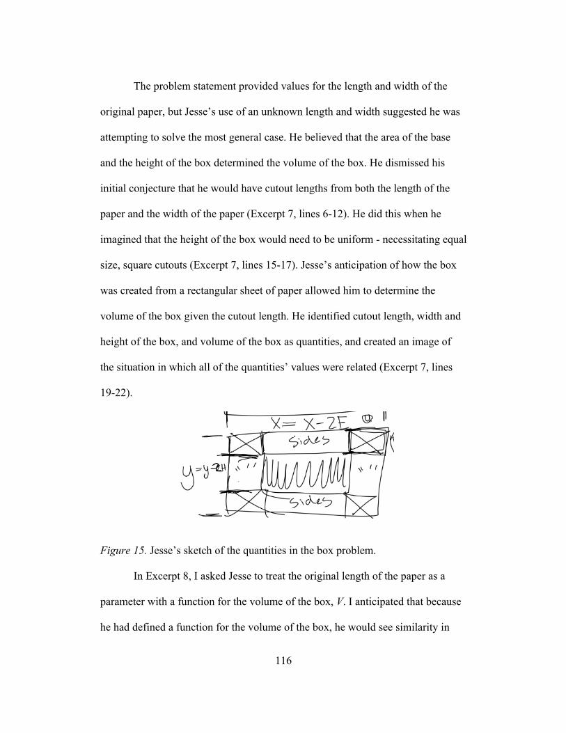
116
The problem statement provided values for the length and width of the
original paper, but Jesse’s use of an unknown length and width suggested he was
attempting to solve the most general case. He believed that the area of the base
and the height of the box determined the volume of the box. He dismissed his
initial conjecture that he would have cutout lengths from both the length of the
paper and the width of the paper (Excerpt 7, lines 6-12). He did this when he
imagined that the height of the box would need to be uniform - necessitating equal
size, square cutouts (Excerpt 7, lines 15-17). Jesse’s anticipation of how the box
was created from a rectangular sheet of paper allowed him to determine the
volume of the box given the cutout length. He identified cutout length, width and
height of the box, and volume of the box as quantities, and created an image of
the situation in which all of the quantities’ values were related (Excerpt 7, lines
19-22).
Figure 15. Jesse’s sketch of the quantities in the box problem.
In Excerpt 8, I asked Jesse to treat the original length of the paper as a
parameter with a function for the volume of the box, V. I anticipated that because
he had defined a function for the volume of the box, he would see similarity in

117
generating the graph of V(x) where original length was a parameter and the
difference function h(x) = a(f(x)-g(x)).
Excerpt 8 (Day 4 of TE, 00:00:25)
EW: Now, we just considered a graph of volume of the box as a function of 1
the cutout length made from the sheet of paper. If we made the length 2
of the sheet of paper a parameter, and varied the parameter, how do 3
you think that would affect the behavior of the function for the volume 4
of the box? 5
Jesse: Well, hmm. I think that would affect only the output, or the volume of 6
the box, so you would see the hump increase or decrease (Figure 16). 7
Weird, I’m mostly right, but when the parameter for length [points to 8
the length of the original sheet of paper] gets less than 12 when the 9
width is 12, the zeroes of the graph change because the length 10
constrains the volume as it is less than the width (Figure 17). 11
EW: I’d like you to think about this like we did in the last example. If we 12
imagine the parameter sweeping out a surface, how do you think this 13
function [for volume of the box] might behave? 14
Jesse: Well, again, I would treat the volume like the z-axis, the cutout like the 15
x-axis and the like the y-axis. I could imagine the function from two 16
ways, either treating x [the cutout length] like a parameter and the 17
length of the original sheet like a variable or y like a parameter and x 18
like a variable. Either way, I could sort of imagine the tracing out 19

118
happening, but this function is a little weird so I would want to use GC 20
to do that instead of just guessing. 21
EW: So, you talked about referring to these views as perspectives, what 22
perspective would those be? 23
Jesse: Well, one would be the z-x and one would be the z-y, like the volume-24
cutout perspective and the volume-length perspective. In both cases, 25
I’d guess you see humps that open downward, which probably comes 26
from some interaction of all the variables. 27
Jesse anticipated that varying the length of the original paper would only
affect the volume of the box (Excerpt 8, lines 6-8), which would make the hump
(a feature of the graph he noted), move vertically (Excerpt 8, lines 7-8). I asked
him to anticipate the behavior of the volume function where the length of the
paper was represented on a third axis. He used his notion of perspectives to think
about the graph. He focused on volume-cutout, which was like the z-x
perspective, and volume-length, which was like the z-y perspective.
Figure 16. Jesse’s graph of the two-variable box problem function.

119
Figure 17. Jesse’s screen as he described the zeroes changing.
Jesse visualized the function’s graph in space from each perspective, but I
believed he was not attending to generating the function by using level curves, or
the x-y perspective. This resulted in his guessing at how the perspectives fit
together (Excerpt 8, lines 26-27), which he referred to as an interaction of
variables. By interaction, I believed he meant he was trying to anticipate how the
z-x and z-y perspectives “fit” together as objects to create a surface in space.
In Excerpt 9, I explored my conjectures about his use of perspective by
asking him to anticipate the graph of the volume function if the y-axis represented
the area of the base of the box. I asked him to place a function of x on the y axis
(area) to gain insight into how he would think about the effect of changing the
quantity represented on an axis on the surface in space. I intended to promote a
focus on the quantities represented on the axes as critical for interpreting the
“shape” of a surface in space.
Excerpt 9 (Day 5 of TE, 00:00:04)
EW: You just described the graph of the function where the length of the 1
original sheet of paper was represented on the third axis. Suppose that 2

120
you treated the third axis as representing the area of the base of the 3
box. How would that affect the graph of the function? 4
Jesse: Well, let’s see, so I am still keeping volume as like the z variable, 5
cutout length is the x variable, and now base area is the y variable. 6
Well, isn’t z just coming from multiplying x and y? Yeah, just 7
multiplication I think. Okay, well, look at the z-x perspective, then y is 8
a parameter, so we just sweep out a linear function, same thing from 9
the z-y perspective. Sweep out two linear functions, and then sort of 10
bring their behavior together. 11
EW: What do you mean, bring their behavior together? 12
Jesse: Well, if I look overhead, I have to think about how to combine the z-x 13
and z-y perspectives, this is kind of like the x-y look. 14
EW: Can you think about the x-y perspective like you do the others? 15
Jesse: Mmm, process of elimination, z becomes the parameter then? 16
EW: Sure, let’s work with that. 17
Jesse: Okay, well, then you are going to be sweeping out things like y = 1/ x18
Jesse focused on generating the function from both the z-x and z-y
perspectives when thinking about the effect of changing the quantity represented
on the y-axis. He accurately described a linear function tracing out a surface, from
both the z-x and z-y perspectives (Excerpt 9, lines 5-11), which suggested to me,
in the moment, that he was focusing on the surface as a representation of a
relationship between quantities. I believed this because he was unsurprised by the

121
difference in the surface (compared to when y was cardboard length) when he
graphed it in GC. I was also surprised that he used level curves by treating z as a
parameter value because he had focused on “eyeballing” how the z-x and z-y
perspectives fit together up to that point (Excerpt 9, lines 13-14, 18).
Jesse’s work on the box problem during Days 4 and 5 suggested to me that
his use of perspective relied on his associating a graph with an image of how it
was generated using covariation. Whenever he thought about a surface, he
imagined that surface constructed by a one-variable function sweeping out in a
plane. This image is similar to visualizing a vertical cross-section moving along
an axis. In the case of the z-x perspective, he imagined thinking about the variable
y as a parameter a, which he could move in increments along the third axis. This
way of thinking allowed him not only to imagine a continuous sweeping out of
cross-sections, but also helped him interpret what those cross sections
represented. Thus, at that time, I believed an association of a surface in space with
a process of covariation used to construct it could characterize expert shape
thinking.
Days 9 and 10 - Non-Quantitative Setting
The first iteration of the teaching experiment sequence intermixed ideas of
function with rate of change tasks. During Days 6, 7 and 8 we focused on
discussing rate of change. This was due to the original task trajectory. We
resumed talking about the graphs of two-variable functions on Days 9 and 10. I
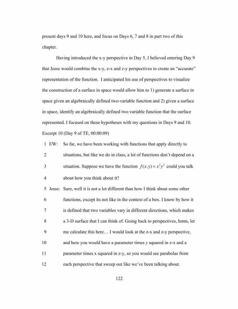
122
present days 9 and 10 here, and focus on Days 6, 7 and 8 in part two of this
chapter.
Having introduced the x-y perspective in Day 5, I believed entering Day 9
that Jesse would combine the x-y, z-x and z-y perspectives to create an “accurate”
representation of the function. I anticipated his use of perspectives to visualize
the construction of a surface in space would allow him to 1) generate a surface in
space given an algebraically defined two-variable function and 2) given a surface
in space, identify an algebraically defined two variable function that the surface
represented. I focused on these hypotheses with my questions in Days 9 and 10.
Excerpt 10 (Day 9 of TE, 00:00:09)
EW: So far, we have been working with functions that apply directly to 1
situations, but like we do in class, a lot of functions don’t depend on a 2
situation. Suppose we have the function f (x, y) = x2y2 could you talk 3
about how you think about it? 4
Jesse: Sure, well it is not a lot different than how I think about some other 5
functions, except its not like in the context of a box. I know by how it 6
is defined that two variables vary in different directions, which makes 7
a 3-D surface that I can think of. Going back to perspectives, hmm, let 8
me calculate this here… I would look at the z-x and z-y perspective, 9
and here you would have a parameter times y squared in z-x and a 10
parameter times x squared in z-y, so you would see parabolas from 11
each perspective that sweep out like we’ve been talking about. 12
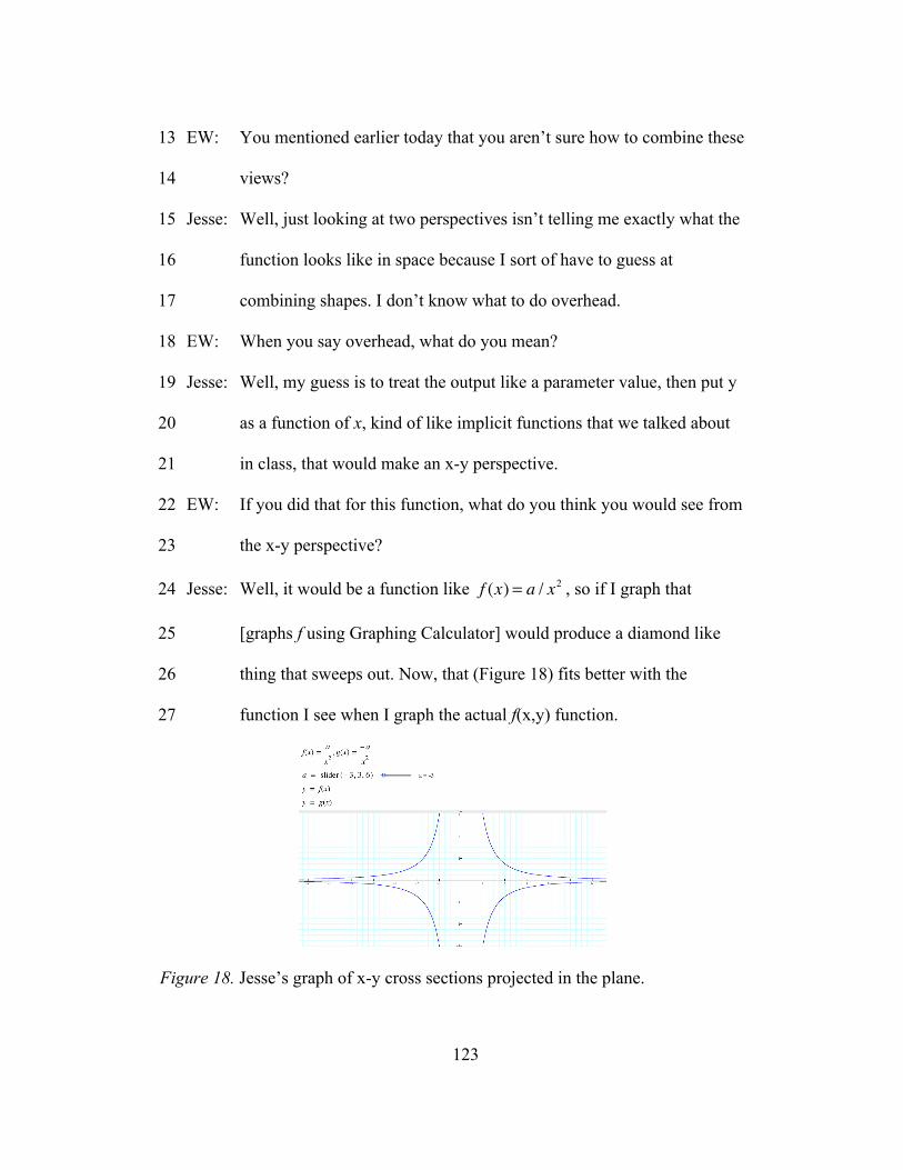
123
EW: You mentioned earlier today that you aren’t sure how to combine these 13
views? 14
Jesse: Well, just looking at two perspectives isn’t telling me exactly what the 15
function looks like in space because I sort of have to guess at 16
combining shapes. I don’t know what to do overhead. 17
EW: When you say overhead, what do you mean? 18
Jesse: Well, my guess is to treat the output like a parameter value, then put y 19
as a function of x, kind of like implicit functions that we talked about 20
in class, that would make an x-y perspective. 21
EW: If you did that for this function, what do you think you would see from 22
the x-y perspective? 23
Jesse: Well, it would be a function like f (x) = a / x2 , so if I graph that 24
[graphs f using Graphing Calculator] would produce a diamond like 25
thing that sweeps out. Now, that (Figure 18) fits better with the 26
function I see when I graph the actual f(x,y) function. 27
Figure 18. Jesse’s graph of x-y cross sections projected in the plane.

124
Jesse found it natural to think about unspecified quantities as he had when
the quantities were specified, as in the box problem (Excerpt 10, lines 5-7). He
imagined generating the graph from the z-x and z-y perspectives, which would
produce “parabolas from each perspective that sweep out” (Excerpt 10, lines 11-
12). When he began imagining how to “combine” these perspectives, he described
his difficulty with imagining what the graph would look like from “overhead”. He
relied on the level curves projected into the x-y plane. He defined the generating
function f (x) = a / x2 , which he believed would sweep out a “diamond like thing”
above the x-y plane, which appeared to fit with the surface he generated (Figure
19) in Graphing Calculator (Excerpt 10, lines 24-27). This excerpt suggests that
Jesse was beginning to think about the graph of a two-variable function by
generating it from what he would call “side” perspectives (z-x and z-y), and an
“overhead” perspective (x-y), which is like a level curve projected in the x-y
plane. In the moment, I wrote that Jesse appeared to think about the x-y
perspective as a way to generate a more accurate graph because he could “check”
how the z-x and z-y perspectives interacted. I understood him to mean that he was
not guessing at how “parabolas” from z-x and z-y perspectives combined. Instead,
he described the interaction of those parabolas from each perspective by
projecting x-y cross sections in the plane.
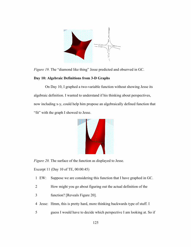
125
Figure 19. The “diamond like thing” Jesse predicted and observed in GC.
Day 10: Algebraic Definitions from 3-D Graphs
On Day 10, I graphed a two-variable function without showing Jesse its
algebraic definition. I wanted to understand if his thinking about perspectives,
now including x-y, could help him propose an algebraically defined function that
“fit” with the graph I showed to Jesse.
Figure 20. The surface of the function as displayed to Jesse.
Excerpt 11 (Day 10 of TE, 00:00:45)
EW: Suppose we are considering this function that I have graphed in GC. 1
How might you go about figuring out the actual definition of the 2
function? [Reveals Figure 20]. 3
Jesse: Hmm, this is pretty hard, more thinking backwards type of stuff. I 4
guess I would have to decide which perspective I am looking at. So if 5

126
this is z-y, it looks like it could have been generated by a moving 6
parabola. Then in z-x, well, it looks linear in some places, so maybe 7
produced by a moving linear function. But, wait, on top the function 8
looks a little strange, so I would have to do some more exploring. With 9
all of these, I would have to be able to look at points and check they fit 10
with a parabolic function, or linear I think. 11
EW: So, based on what you have said, how might you define the function? 12
Jesse: My best guess is like ay2 from z-y and bx from z-x, so a parameter 13
times xy214
Jesse defined the z-y plane to fix an orientation on the graph (Excerpt 11,
line 6), and conjectured that perspective was generated from a moving (or
sweeping out) parabola. Once he defined the z-y plane, this created the z-x plane,
which he believed was produced by a moving (or sweeping out) linear function.
While Jesse attended to the shapes associated with the graph in each perspective
(Excerpt 11, lines 7-10), he held in mind that the graph actually represented a
linear or quadratic relationship between quantities. I believed that Jesse was able
to describe the algebraic form of the two-variable function f (x, y) = xy2 (Excerpt
11, lines 13-14) because he was thinking about one-variable functions in the plane
generating the surface from the z-x and z-y perspective.
Part I Conclusions
I began the teaching experiment with a naïve notion of importance of
shape thinking. However, my analyses revealed that expert shape thinking was at
127
the heart of my model for Jesse’s ways of thinking about 2-variable functions. In
this section, I describe the foundations of my model for his thinking that resulted
from both my intra teaching experiment and retrospective analyses.
Expert shape thinking. It is important to note that shape thinking is an association the student has
when thinking about a graph. Thus, shape thinking as a construct is not “good” or
“bad”. Expert shape thinking consists of associating a function’s graph as a
emergent representation of quantities having covaried, where those quantities’
values are represented on the axes in Cartesian coordinates. When Jesse, an expert
shape thinker, attended to the shape of a graph, such as describing a “hump” or a
“valley”, he appeared to associate those features as the result of tracking a
multiplicative object composed of two or more quantities’ values. His
understanding that the graph was created by the quantities’ values represented on
the axes displayed a critical component to expert shape thinking, attention to the
axes. By focusing on the axes and variables’ variation on them, Jesse was able to
imagine how the graph of a given two-variable function had been generated using
a coupling of the quantities in the situation.
Generating the domain of the function.
My analyses suggested that Jesse’s expert shape thinking supported his
development of visualizing graphs of one-variable functions having been swept
out (producing a completed graph) and then those completed graphs being swept
out to produce surfaces in space from various “perspectives”. When Jesse referred
128
to thinking about a perspective, he imagined a sweeping out occurring. By
sweeping out, I mean that he imagined a two-variable function as a one-variable
function by treating one of the two variables as a parameter and imagined that
parameter iterating through a set of values, which produced the sweeping out.
Jesse’s understanding of a function in the plane sweeping out a surface in space
suggested he was using expert shape thinking. Jesse saw the sweeping out as the
tracing out of a relationship between variables representing quantities’ values. He
described how he thought about both one and two-variable functions’ graphs as
the result of programming “a generating object”. Jesse’s meaning of
“programming” seemed to be that he envisioned putting into his imagined object
the power to covary its coordinates on its own. By “programming” the object,
Jesse seemed to be saying, “and I can imagine this object behaving like it should
without me having to think of what it should do”. Programming the object thus
resulted from attending directly to the quantities values represented on the axes,
which is a component of expert shape thinking.
This instructional sequence used functions whose graphs can be
envisioned by the sweeping out of a plane that contains a graph. This way of
thinking, in effect, generates the x-y plane by sweeping a line through it parallel to
one of the axes. But there are many ways of generating the domain. Another way
is to imagine pre-images of level curves—the set of points (x,y) in the x-y plane
that map into z = c. For example, the graph of f (x, y) = cos(x2 + 3y2 ) is most
easily imagined by thinking of generating the x-y plane by varying c in

129
x2 + 3y2 = c, c ! 0 . Jesse constructed the domain of the function f (x, y) = x2y2 by
considering pre-images of level curves. However, my analyses revealed that
Jesse’s way of thinking about functions’ surfaces being generated by a sweeping
of a plane that contained a graph was productive for the types of functions in this
instructional sequence.
Part II: Jesse’s Ways of Thinking about Rate of Change
Part two of this chapter focuses on Jesse’s ways of thinking about rate of
change in space. Table 17 provides an outline of tasks and dates, on which I base
my analyses in Part II. I drew a number of excerpts for Parts I and II from the
same day, but the time demarcations show when each discussion occurred.
Table 17
Jesse’s Rate of Change Task Sequence.
Task Description Date (Day) Car A – Car B: Interpreting Meaning of the Graph 3/15/2011 (2) Car A – Car B: Measuring Rate of Change Using
the Graph 3/15/2011 (2)
Treating a as a Third Axis 3/17/2011 (3)
Box Problem: Box Construction and Treating Parameters as Variable
3/21/2011 (4)
Box Problem: Interpreting the Meaning of Rate of
Change at a Point in Space 3/23/2011 (5)
Box Problem: Measuring the Rate of Change at a Point in Space
3/23/2011 (5) 3/25/2011 (6)
Drivercost Problem: Parameters as Variables and Rate of Change 3/25/2011 (6)
Generalized Rate of Change Function and Direction
3/27/2011 (7) 3/29/2011 (8)

130
My interactions with Jesse in tutoring suggested that he thought about rate
of change as tracking the value of a quotient that compared an change in a
function’s input to the change in the function’s output. During an exam review, he
said originally he thought rate of change as another way to talk about the slope of
a function, and did not understand why the instructor focused on talking about
rate of change as more than just the slope of a function. He said he had an “ah-ha”
moment when he realized rate of change was a function that tracked how “fast
one quantity was changing with respect to the other”. Jesse appeared to think
about rate of change as the multiplicative comparison of changes in the input and
output of the function. I anticipated that this way of thinking could be naturally
extended to think about a rate of change in space.
Key Terms and Definitions
This teaching experiment focused on rate of change, but used terms with
which the reader may not be familiar. In the following excerpts, Jesse describes
functions expressed in open and closed form. A function is expressed in closed
form when it is defined succinctly in terms of familiar functions, or algebraic
operations on familiar functions. The function f defined as f (x) = xk
k!k=0
!
" is in
open form, whereas f defined as f (x) = ex is in closed form. You will see Jesse
referring to rate of change functions in open and closed form. The function rf
defined as rf (x) =f (x + h)! f (x)
h, where x varies and h is fixed, is in open form.
This function, first used by Tall (1986), gives the average rate of change of f over

131
the interval [x, x + h] for all values of x in f’s domain. rf approximates the
derivative of f for suitably small values of h. This simultaneous variation of x and
rf is illustrated by the sliding calculus triangle, to which Jesse referred to
numerous times in our sessions (Figure 21). It must be noted that the calculus
triangle is a mnemonic for thinking about measuring rate of change that Patrick
Thompson has used for many years in both teaching and research. Though we
recently submitted a paper about calculus triangles (Weber et al., in press) to
characterize the images Thompson intended the calculus triangle to engender in
students, Thompson originally conceived of the term calculus triangle and its
associated images.
Figure 21. The calculus triangle slides through the domain of the function (from
Weber, Tallman, Byerley, and Thompson, in press).
In order to generate outputs for the average rate of change function, one
measures the quantity f(x+h) – f(x) in units of h and systematically associates this
output value with x, the left endpoint of the interval [x, x + h]. Accordingly, a
point on the rate of change function can be interpreted as (x, f(x+h) – f(x) units of

132
h) (see Figure 21). Then, as x varies throughout the domain of the function, this
point traces out the rate of change function (Figure 22).
Figure 22. The sliding calculus triangle generates the average rate of change
function over intervals of size h.
Lastly, when Jesse referred to the closed form rate of change, he was
describing the “exact” rate of change function in which h is indistinguishable
from zero. Closed form rate of change often resulted from using “rules of
derivatives” or “going through the open form calculations and making h
essentially zero”, according to Jesse.
Day 2 - Car A-Car B Activity The episodes focusing on Jesse’s ways of thinking about rate of change
were intermixed with tasks related to graphs of function. The Car A-Car B
activity (described in chapter three, Figure 23) occurred on Day 2. I anticipated
that Jesse would focus on a correspondence point that was “programmed” using
the car’s speed and the amount of time elapsed. I conjectured that Jesse would
focus on tracking the quotient of the change in the car’s speed over a certain
interval of time, and would repeat that process over equivalent intervals of
rf (x)

133
elapsed time to describe the car’s acceleration as increasing or decreasing. Also,
given Jesse’s focus on using open form rate of change, I thought that he would
describe that a more accurate rate of change of the car’s speed with respect to
time could be generated by making h very small.
Figure 23. The graphs of Car A and Car B’s speed as a function of time.
Excerpt 12 (Day 2 of TE, 00:00:07)
EW: So if we look at the graph of Car A and Car B (Figure 23), where do 1
you imagine they are after one hour in relation to each other? 2
Jesse: They look like they are at the same location. The lines seem to 3
intersect there. Hmm, we have speed, and time, oh duh, stupid, it’s 4
speed and time not distance so the top car is further than the other one. 5
EW: So Car A is further along than Car B you think. What can you say 6
about their rates of change? 7
Jesse: Well, this is a rate of change graph because we are talking about 8
speed. So if you zoomed in like we did in class, you would probably 9
see a bunch of connected linear segments representing average speed 10
over small intervals. 11

134
EW: What would it mean if they were linear segments, as you said? 12
Jesse: It would be a bunch of constant speeds, coming from average speed, 13
over an interval of h, which is really small probably. In theory, we 14
wouldn’t see the segments if h were zero, but in that case, we would 15
not have a graph.16
Jesse first interpreted the graph as a distance-time graph, and hence
believed the cars were at the same location because the graphs crossed after one
hour (Excerpt 12, line 4). He caught his error when he reread the labels on the
axes, and noted one car must be in front of the other after one hour (Excerpt 12,
lines 4-5). I inferred that his realization resulted from thinking that the two cars
started at the same place and, after starting, one car always went faster than the
other so they could not be in the same location.
Jesse described the graph as tracking average speed (Excerpt 12, line 10).
He anticipated zooming in on the graph to see connected linear segments
representing the average speed of the car over small time intervals (Excerpt 12,
lines 9-11). Jesse’s response suggested that he was thinking about speed as a rate,
which itself was created by comparing a change in distance with a change in time.
As a result of this comparison of changes, Jesse emphasized the graph must be
linear segments because speed could not be measured without constructing
average speeds of the car over small intervals of time. In order for the graph to be
made of average speeds over small intervals, the graph must represent a step
135
function. The linear segments would come from the distance-time graph and
graphing average speed over those intervals.
In Excerpt 13, Jesse described measuring the rate of change of speed with
respect to time. He focused on using a “consistent h” (i.e. fixed change in x) to
measure the rate of change in the domain of the given function. He imagined
using the open form rate of change with a small, but fixed value of h to
approximate the rate of change function, because making h zero in the context of
a graph was impossible (Excerpt 12, line 16). I believed that Jesse’s description of
a consistent h allowed him to compare differences in the change in the output. I
believed, in the moment, that using a consistent h was much like using the
calculus triangle to think about the rate of change function. In order to test these
conjectures, I asked Jesse to compare the rates of change of Car A and Car B.
Excerpt 13 (Day 2 of TE, 00:00:28)
EW: Earlier I was hoping we could compare the rates of change of the cars. 1
Jesse: Well, the rate of change of the information here would be the 2
acceleration of the cars, not the speed, but you would just give h a 3
number, probably like .01, then starting from zero seconds, take the 4
difference in speed every .01 seconds and divide that by .01. It’s pretty 5
much the open form rate of change we have talked a lot about in class, 6
sort of like the calculus triangle where you use a bunch of them. 7
EW: Could you say more about the calculus triangle and the open form? 8

136
Jesse: Well, from what I understand, you basically fix a slider value of h, 9
then take successive differences. In the calculus triangle, you fix the 10
length of the bottom leg, then let it slide through whatever you are 11
trying to find the rate of change of, or for I guess. I’m more 12
comfortable with using the open form rate of change though. 13
EW: So if the open form rate of change produced a value of 3.45 for an h-14
value of .01, what would that mean? 15
Jesse: Well, the constant rate of change of speed would be 3.45 over that 16
small interval, so every time you add something to x, the y value goes 17
up 3.45 times that much, theoretically. 18
EW: Theoretically? 19
Jesse: Well, it doesn’t actually change constantly usually, it’s just an average 20
rate of change that is like a constant rate when calculated. 21
Jesse anticipated he would need to fix the change in time to compare the
rate of change of the each car’s speed with respect to time (Excerpt 13, lines 3-4),
which would allow him to compare the difference in speed every time .01 seconds
elapsed (Excerpt 13, lines 4-5). He believed fixing h was related to calculus
triangles and the open form rate of change function (Excerpt 13, lines 5-6). His
description of using a bunch of them (Excerpt 13, line 7) and letting the calculus
triangle slide (Excerpt 13, lines 10-12) support that he was thinking about many,
small, calculus triangles existing in the domain of the function (Figure 24).
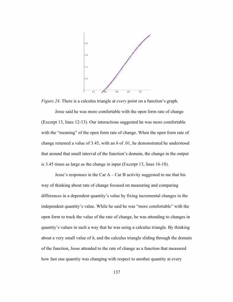
137
Figure 24. There is a calculus triangle at every point on a function’s graph.
Jesse said he was more comfortable with the open form rate of change
(Excerpt 13, lines 12-13). Our interactions suggested he was more comfortable
with the “meaning” of the open form rate of change. When the open form rate of
change returned a value of 3.45, with an h of .01, he demonstrated he understood
that around that small interval of the function’s domain, the change in the output
is 3.45 times as large as the change in input (Excerpt 13, lines 16-18).
Jesse’s responses in the Car A – Car B activity suggested to me that his
way of thinking about rate of change focused on measuring and comparing
differences in a dependent quantity’s value by fixing incremental changes in the
independent quantity’s value. While he said he was “more comfortable” with the
open form to track the value of the rate of change, he was attending to changes in
quantity’s values in such a way that he was using a calculus triangle. By thinking
about a very small value of h, and the calculus triangle sliding through the domain
of the function, Jesse attended to the rate of change as a function that measured
how fast one quantity was changing with respect to another quantity at every
138
point in the domain of the function, and he appeared to do so multiplicatively. His
responses in Excerpt 13 (lines 20-21) supported that he was thinking about open
rate of change and calculus triangles as measuring average rate of change. His
interpretation of the graph of the Car A- Car B graph also supported that as he
thought about average rate of change as a constant rate of change.
Day 3 - Sweeping Out a One-Variable Function The Car A-Car B (Day 2) episode occurred prior to generating the surface
of a two-variable function (Day 3). I used Day 3 to test two conjectures: 1) I
believed Jesse was thinking about open form rate of change as more “reliable”
because it used the original function in its calculations, 2) I anticipated it would
be critical for Jesse to think about f(x,y) changing with respect to both x and y, so
that he could imagine partial rates of change using calculus triangles, which could
support developing directional rate of change. After we discussed the sweeping
out of a one-variable function, I asked Jesse to describe how he would think about
the rate of change of the difference function f (x) = x3 ! 2x .
Excerpt 14 (Day 3 of TE, 00:00:22)
Jesse: If I go back to the function we just talked about sweeping out and 1
thinking with depth. I could use the open form on it, with a small value 2
of h which would graph a rate of change with linear segments, or I 3
could calculate the closed form rate of change, three x squared minus 4
two, using rules. 5
EW: Could you say more about open and closed form? 6

139
Jesse: Well, open form is more directly tied to the function because it 7
depends on the original function every time you calculate a value, but 8
closed form is like an open form for when h is zero, which it can’t 9
actually be. Like I said, umm, closed, no, open form has linear 10
segments, but the closed form is exact, it won’t have those linear 11
segments because it doesn’t use an average. 12
EW: So why use both? 13
Jesse: You don’t always know the rule to calculate the rate of change 14
function, or sometimes its just impossible. If you make h small 15
enough, it gets super close to the closed form anyway, so it’s a good 16
approximation. The closed form doesn’t really mean the same thing as 17
open form, which stands for a constant rate. Closed form kind of just 18
is, it just is the value, not an approximation.19
Jesse described the rate of change of h(x) by using open or closed form
rate of change. He believed that open form rate of change was directly constructed
from the function itself, but could not measure an “exact” rate, while the closed
form rate of change represented the value of the open form if h was
indistinguishable from zero (Excerpt 14, lines 7-12). Jesse appeared to think that
the open form change was applicable to all functions with which he was familiar,
while closed form rate of change was sometimes intractable because a “rule” was
not available or the algebra was too complex (Excerpt 14, lines 14-15) to calculate
a rate. Jesse’s responses indicated to me, in the moment, that he was thinking

140
about the values of open and closed form rates of change as different when h is
large, but equivalent when h becomes extremely small. However, he thought
about the meaning of open and closed form rate of change as different because
closed form was exact, while open form was an average rate of change over an
interval of the function’s domain.
Minutes after this discussion, I asked Jesse to describe what it would mean
to describe a rate of change of a function represented in space (as we had just
generated a function’s graph in space using graphing calculator). I wanted to
understand how my model for Jesse’s ways of thinking might extend to the notion
of rate of change at a point, or over an interval, in space. This excerpt comes from
the end of Day 3.
Excerpt 15 (Day 3 of TE, 00:00:55)
EW: So you just worked on starting to think about functions using depth, 1
and created some ideas of how to think about surfaces in space. If you 2
look at the surface in space we just generated, how do you think rate of 3
change is the same or different from a function of one variable? 4
Jesse: Well it’s actually pretty strange, because now you have to account for 5
an output and two variables, so it’s like an output is changing with 6
respect to two things. 7
EW: Suppose we had defined a two variable rate of change function, 8
whatever that might be, and its output was 1.23. What would that 1.23 9
mean? 10
141
Jesse: Oh man, well, it would probably be a constant rate of z with respect to 11
x and y, which is pretty weird, because how can it be changing with 12
respect to both variables at once? My first guess is that we are going to 13
have another open form rate of change function. I guess, maybe, you 14
have two rates of change, one from z-x and one from z-y [referring to 15
perspectives], and you add them together in some way that might make 16
sense.17
Jesse’s was thinking about the dependent variable changing with respect to
two independent variables simultaneously (Excerpt 15, lines 5-7). I believed, in
the moment, that he was struggling with what a rate of change in space would
mean. In response, I asked him to interpret the value of a theoretical rate of
change function in space (Excerpt 15, lines 5-7). His description of a constant rate
of z with respect to x and y (Excerpt 15, lines 11-13) appeared to be consistent
with his meaning for rate of change of a one-variable function. His reliance on
what he knew about rate of change in one variable helped him describe two rates
of change occurring from the z-x and z-y perspectives, notions which he had just
started developing (Excerpt 15, lines 15-17). Jesse was struggling to think about
how a number could represent how fast a quantity was changing with respect to
two different independent variables. Yet his description of two rates of change
occurring simultaneously in different planes suggested that thinking about partial
rates of change, and thus, rate of change in a direction, could be tenable.
142
Between Day 3 and 4: Jesse’s Reflections Minutes after our Day 3 discussion ended, Jesse said that he had some
ideas about defining a two-variable open form rate of change function. I
encouraged him to submit his responses to me prior to our next session, Day 4. I
asked him to consider the following three questions for each of his “ideas”.
a) Why do you think this function is a possibility for the rate of change function?
b) Suppose that the result of the calculation in your conjecture was 243. What
would 243 represent?
c) Are there any issues with your conjecture that make you question its accuracy?
The following is what Jesse sent by email, prior to our meeting on Day 4.
The following descriptions were written by Jesse. He produced four
“conjectures”, and answered the three questions for each conjecture. I discuss my
interpretation of each of his responses, and how I planned to use them in Day 4 of
the teaching experiment.
1)
a) The reason I think this could be a possibility for graphing the 3
dimensional representation of V(x,y) is because when we want to graph the rate
of change of a 2 dimensional function the form is [V (x + h)!V (x)] / h because
you want to see the change in V(x) over the interval of x to x+h over a unit of h.
However when we are representing the rate of change in 3 dimensions the
reason this function could be a possibility is because we’re not only looking at
the change that happens to V(x,y) from x to x+h but also the change that is
rV (x, y) =V (x + h, y + h) !V (x, y)
h

143
happening to V(x,y) from y to y+h Another way of expressing why I think we
should try to account for the change in y over an interval of y to y+h is because
there is change happening not only the x-z axis but on the y-z axis.
b) If the answer to this calculation was 243 it would be saying that over an
interval of x to x+h and an interval of y to y+h there would be an average rate of
change of 243. So since we’re talking about volume in a box it would mean that
if an imaginary box increased its volume by 243 from x to x+h and y to y+h that
it would account for the same amount of change over the given interval.
c) The thing about this function that I’m not sure about is trying to also take
into account the change in y over the interval of h and the affects it has on
V(x,y) , I feel that I need to represent this change in y on the graph but I’m not
sure that this is the way to do so.
I believed Jesse’s first conjecture indicated he was thinking about comparing
a change in the dependent variable that resulted from adding h to both x and y.
However, it was not clear what he imagined h to represent, and did not explain
why he anticipated adding the same value of h to x and y.
2.
a) The reason I think this function is a possibility is because maybe in
accounting for the rate of change over the interval of x to x+h and being given a
certain value of y maybe this will also show the change in y on the graph. Or
for example when we were dealing with the rate of change of this function when
it was two dimensional we did not have to account for the rate of change of the
rV (x, y) =V (x + h, y) !V (x, y)
h

144
parameter a, so maybe the three dimensional graph will act the same and
account for the change in y by itself.
b) If the result of this function was 243 then it would be saying that over the
interval of x to x+h they’re an average rate of change of 243. This also is
assuming that by showing the rate of change from x to x+h it also accounts for
the change in y.
c) Since in this function we don’t try to account for change in y from y to y+h
we are assuming that its already going to be shown since it needs to be
accounted for in a 3D graph. This is definitely something I’m not sure about but
at the same time the exact reason why I think it’s a possible solution.
I believed his second conjecture suggested he was thinking about varying x
while fixing the value of y, creating a rate of change in the z-x perspective. In
this case, the value of h he was thinking about was the same as if he had been
describing a one-variable rate of change function.
3.
a) I think the reason that I suggested this function as a possibility is because I
felt it was saying the same thing as the function from problem 2. However I
honestly don’t think this would work since V(x) uses a parameter a to find the
volume where V(x,y) uses y in place of a. Even though these two functions are
solving for volume they are not defined in the same terms. I don’t trust this one
anymore.
rV (x, y) =V (x + h) !V (x)
h

145
4.
a) The reason I thought that this could be a possibility is because much like
the function from problem one this would account for the change happening in x
and for the change in y. The only difference here is that the input x in this
function stands for a the cut out length which can be in feet or inches or
something along those lines that also means that h must be in the same units of
measurement. So the reason for adding w to y instead of h is because maybe y
isn’t a value that represents something in the same units of measurement as x
and h.
b) Just like in problem one this would mean that in the average rate of change
over the intervals of x to x+h and y to y+w would be 243.
c) After thinking about question b for this function I think my biggest area of
concern is adding w. I wouldn’t know how to determine what w should be,
should I give w the same value as h? Not only that but what would 243 from
question b really represent when I have x over an interval of one value and x
increasing by an interval of another value, I wouldn’t know if it was the
combined increase of both the change in x and y or something else.
After doing this exercise I’m thinking that my second idea still seems like the
best solution to me. The reason for this is because I think it has the best way of
representing the change happening over x and in y, since it would be solving the
rate of change in much the same way we did for the two-dimensional graph and
still account for the value of y.
rV (x, y) =V (x + h, y + w) !V (x, y)
hw

146
I believed Jesse’s fourth conjecture was almost identical to his first, except
he imagined adding different amounts to x and y, as indicated by his use of h
and w instead of simply h. However, Jesse did not explain his rationale for using
the denominator hw.
Jesse’s three rate of change conjectures (I considered his response to the
third to indicate he did not find it valid) indicated that he was struggling with how
to think about a quantity’s value changing with respect to the value of two other
quantities. I believed that each of Jesse’s conjectures could be referenced to
support him in thinking about a rate of change in a direction in space. Together,
his conjectures indicated to me that he was struggling with 1) how to combine or
use rates of change in the z-x and z-y direction and 2) how to define the
denominator of the rate of change function so it would fit with the meaning he
created for a two-variable rate of change function. I used the context of the box
problem to explore these conjectures and to build supports for helping Jesse think
about rate of change in a direction in space.
Days 4-5: Box Problem and Rate of Change I anticipated that because of his rate of change conjectures, it would be
key to support Jesse in thinking about 1) partial rates of change as occurring
simultaneously in the domain of the two-variable function, and 2) imagining
making the changes in quantities represented on the x and y axes small in tandem
in order to approximate the rate of change of the volume of the box with respect
to cutout length and base area. I believed that these ways of thinking would help

147
him imagine rate of change in a direction, in which the changes in x and y occur
simultaneously and depend on each other. Thus, this session focused on
supporting Jesse in conceptualizing the two-changes problem. I began Day 4 by
asking Jesse to reflect on the conjectures he had developed about the rate of
change of a two-variable function.
Excerpt 16 (Day 4 of TE, 00:00:03)
EW: I’d like to focus on some of the conjectures that you worked on after 1
our last meeting. You said you’ve had a chance to think more about it. 2
Jesse: Yeah, well, I really liked conjecture 2, and now I think it’s important 3
because it tells me about the rate of change from a specific 4
perspective. It is like holding y-constant while adding a little bit to x, 5
so it is kind of like making a calculus triangle from the z-x perspective, 6
if that makes sense? 7
EW: I think I am following, but can you say a little more? 8
Jesse: Yeah, well this was for z-x, if I wanted to think about the rate of 9
change in the z-y perspective, I would fix x, then add a little bit to y, 10
and just adjust the function a little bit. Then I have the two rates of 11
change that I am looking for, one for z-x and one for z-y. It’s kind of 12
like making calculus triangles in each perspective, but I’m still 13
working on combining the rate of change functions somehow. 14
EW: I do think I am following now, I just want to clarify, when you use h in 15
the two rate of change functions, are they the same h? 16

148
Jesse: I hadn’t thought about it, but I suppose they don’t need to be because 17
you have control over picking their value.18
Jesse indicated he was thinking about conjecture two as a perspective
dependent rate of change (Excerpt 16, lines 3-6). By perspective dependent, I
mean he was thinking about the z-x perspective by considering the rate of change
of z with respect to x while fixing y, and the rate of change of z with respect to y
while fixing x. He adjusted his conjecture to account for the rate of change in the
z-y perspective (Excerpt 16, lines 9-12). He imagined that perspective dependent
rates of change could be represented by a calculus triangle in each of the z-x and
z-y planes (Excerpt 16, lines 10-14), but said he was unsure how to “combine” the
rates of change (Excerpt 16, lines 17-18). His response suggested two things to
me as we were talking. First, he was focused on the calculation of rate of change,
without first focusing on the meaning of the rate of change that the calculation
would represent. It appeared that he was attempting to accommodate a calculation
in space, not accommodate a meaning that could support a rate of change function
Second, when describing two partial rates of change, he saw the change in x and y
as independent parameter values. By thinking about these as independent
parameter values and focusing only on accommodating a calculation, the two-
changes problem was no initially evident to Jesse.
During a five-minute break in Day 4, I wrote that Jesse was attempting to
calculate an “overall” rate of change. I believed that he would not have occasion
to think about rate of change in a direction without thinking about the x-y
149
perspective to bring about the two-changes problem. I anticipated considering
projections of the function in the x-y plane would allow Jesse to consider the
independence of the changes in x and y, and to consider how directional rate of
change could create a fixed relationship between x and y. The imagery I intended
to support was a calculus triangle sliding in a direction in space. Excerpt 17
followed a discussion between about why he believed the two values for rate of
change, returned by using the calculus triangle in each perspective, needed to be
combined additively or multiplicatively. His responses focused on the idea of
finding a “net change”. Day 4 ended abruptly due to unexpected time constraints
on the interview room. We resumed our discussion on Day 5.
Excerpt 17 (Day 5 of TE, 00:00:04)
EW: You are pretty focused on how to combine these two rate of change 1
functions, before we do any combining, what do they mean 2
individually? 3
Jesse: Well, they are a rate of change for a fixed y, with the z-x open form, 4
and a rate of change for a fixed x, with the z-y open form. They kind 5
of fix one of the variables as a parameter, and focus on a one variable 6
rate of change function. I want to get a net change, coming from z-x 7
and z-y. 8
EW: If you have that information, how are you thinking so that a combined 9
rate of change function becomes important? 10
150
Jesse: Well, in space, you can move in directions other than where one of the 11
variables stays constant, like in a loop, or in a straight line. I need a 12
more general function that accounts for not fixing one of the variables. 13
Ugh, I guess I’m just guessing at how to come up with the function 14
again. 15
EW: You mentioned moving in other directions, and your 4th conjecture 16
was about how to come up with one open form rate of change with and 17
h and w. What adjustments might you make to that conjecture? Let’s 18
work with that. 19
Jesse: For one, I don’t know exactly what to make small, like what is the h 20
for two variables because there are two h’s here. 21
EW: Suppose you thought about walking out in a direction from a point in 22
space, like where the change in y is twice as large as the change in x. 23
Jesse: Well, I would have an h1 and an h2 , but h2 would be twice as big as 24
that h1 . This is kind of like looking from overhead! I just look at 25
changes in y and changes in x. This is kind of like combining the 26
calculus triangles in space in a way. Then as I make either h small, the 27
other one gets small too.28
During our discussion in Excerpt 17, I believed Jesse was focused on a
“net rate of change” (Excerpt 17, lines 7-8), but this kept him from thinking about
the relationship between changes in the x and y. I inferred that the net rate of
change was a way to verbalize his anticipation that he would need to add rates of

151
change from two perspectives. Thus, I believed that to Jesse, “net” meant,
“additively combined”. I decided to build on his fourth rate of change conjecture,
in which he had created parameter values two represent the change in x and the
change in y. His description of not knowing which change to make small (Excerpt
17, lines 20-21), suggested to me that he was thinking about the changes in x and
y as unrelated. He used my suggestion of walking from a point in space as a way
of “combining” (Excerpt 17, line 26) calculus triangles. This appeared to help him
think about a way to find a “net” change. At the end of Day 5, he was focused on
how to relate h1 and h2 (the changes in x and y), which appeared to solve his
dilemma by fixing a relationship between the changes in x and y.
During Day 6, we had the same conversations about the Drivercost
problem as with the box problem. Jesse reached a point where the context
appeared irrelevant to him, and on Day 7, we focused on developing a general,
open form rate of change for a function of two variables. At the beginning of Day
7, I asked Jesse to reflect on his original rate of change conjectures. He noted that
his second conjecture represented a direction in space, just one in which there was
no change in y (z-x perspective) and no change in x (z-y perspective). He said that
his most accurate idea had been the fourth rate of change conjecture because it
accounted for unequal changes in the values of x and y. His new open form rate of
change conjectures was rf (ab)(x, y) =f (x + h1, y +
bah1)! f (x, y)
? . He described
how he could define h2 in terms of h1 by considering a direction in space from

152
the x-y perspective. He attributed his confusion to whether he should include one
or both changes in x and y in the denominator.
Excerpt 18 (Day 7 of TE, 00:00:09)
EW: So how would you define the denominator now, based on what we 1
have talked about? What’s hard about it? 2
Jesse: The denominator was confusing to me at first because I wanted 3
whatever was in the denominator to become small, and I knew two 4
small changes needed to be included. But if I make, umm, the changes 5
depend on each other, then if one of them gets small, the other one gets 6
small as well. I think I could just put one of them in the denominator, 7
maybe h2 , then define h2 in terms of h1 , then it’s like a one variable 8
function that I know how to handle. I guess this is like making and 9
combining two calculus triangles, to make one in a certain direction. 10
EW: Okay, it looks like you have defined the function, now in the context 11
of the box problem, what would a particular value of the function 12
mean? 13
Jesse: The output would be the constant rate of change of the volume with 14
respect to cutout length and base of the box, where those two are in a 15
relationship16
Jesse’s confusion centered on how he could think about changes in both x
and y (Excerpt 18, lines 3-6). It was critical for Jesse to imagine the simultaneous
variation of h1 and h2 and the invariant relationship between them. Thinking

153
about the changes depending on each other (Excerpt 18, line 6), allowed him to
imagine that as one change became small, so did the other (Excerpt 18, lines 6-7).
Anticipating the dependence of the values on each other allowed Jesse to
construct the denominator in the open form rate of change function,
rf (ab)(x, y) =f (x + h1, y +
bah1)! f (x, y)
?. He concluded that h1 alone was a
sufficient denominator because the change in h1 implicitly required a change in h2
to which the change in f(x,y) was compared.
He described the meaning of the open form rate of change function as a
constant rate of change of the volume with respect to two quantities, which are “in
a relationship” (Excerpt 18, lines 14-16). This suggested that he had resolved his
earlier confusion about a dependent quantity changing with respect to two
quantities simultaneously by thinking about the two independent quantities in a
fixed relationship.
Day 8 - Closed Form Rate of Change
Given that the closed form of rate of change in his calculus course
coincided with rules for differentiation, I constructed a way in which to help him
use his idea of perspectives of functions to define a rule of differentiation. In the
following excerpt, I asked Jesse to reflect on his open form rate of change
function, and to discuss how he would think about closed form rate of change for
a function of two variables.
154
Excerpt 19 (Day 8 of TE, 00:00:05)
EW: If you recall, we talked quite a bit about open and closed form rate of 1
change. You mentioned this rate of change function is an example of 2
open form? 3
Jesse: Yep, this is open form, because we are dealing with calculus triangles. 4
The closed form requires some sort of rule. I’m not sure how to deal 5
with it. 6
EW: Let’s use your way of thinking about taking perspectives on functions, 7
if we consider the z-x perspective, for a function like f (x, y) = x2y2 , 8
how would you think about the rate of change? 9
Jesse: Well, from z-x, y is like a parameter, or we fix y, so we can just use the 10
rules we’ve learned in class, it’s like a one variable derivative 11
function, then I can do that for the z-y perspective too. Once I have 12
both of them, I’d probably add them together. 13
EW: How would you check if the closed form was accurate? 14
Jesse: I would make either h1 or h2 , small in the open form rate of change.15
Jesse anticipated he would need a “rule” for the rate of change (lines 5-6).
At my mentioning of thinking with perspective (Excerpt 19, lines 7-9), Jesse
immediately described how thinking about the z-x perspective requires treating y
like a parameter value (Excerpt 19, lines 10-11). In his calculus course, Jesse had
constructed the rule for differentiating a one-variable function with a parameter.
By thinking about a perspective, Jesse made the two-variable function “similar” to
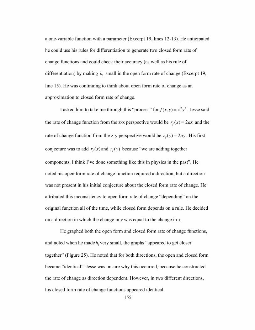
155
a one-variable function with a parameter (Excerpt 19, lines 12-13). He anticipated
he could use his rules for differentiation to generate two closed form rate of
change functions and could check their accuracy (as well as his rule of
differentiation) by making h1 small in the open form rate of change (Excerpt 19,
line 15). He was continuing to think about open form rate of change as an
approximation to closed form rate of change.
I asked him to take me through this “process” for f (x, y) = x2y2 . Jesse said
the rate of change function from the z-x perspective would be rf (x) = 2ax and the
rate of change function from the z-y perspective would be rf (y) = 2ay . His first
conjecture was to add rf (x) and rf (y) because “we are adding together
components, I think I’ve done something like this in physics in the past”. He
noted his open form rate of change function required a direction, but a direction
was not present in his initial conjecture about the closed form rate of change. He
attributed this inconsistency to open form rate of change “depending” on the
original function all of the time, while closed form depends on a rule. He decided
on a direction in which the change in y was equal to the change in x.
He graphed both the open form and closed form rate of change functions,
and noted when he madeh1very small, the graphs “appeared to get closer
together” (Figure 25). He noted that for both directions, the open and closed form
became “identical”. Jesse was unsure why this occurred, because he constructed
the rate of change as direction dependent. However, in two different directions,
his closed form rate of change functions appeared identical.
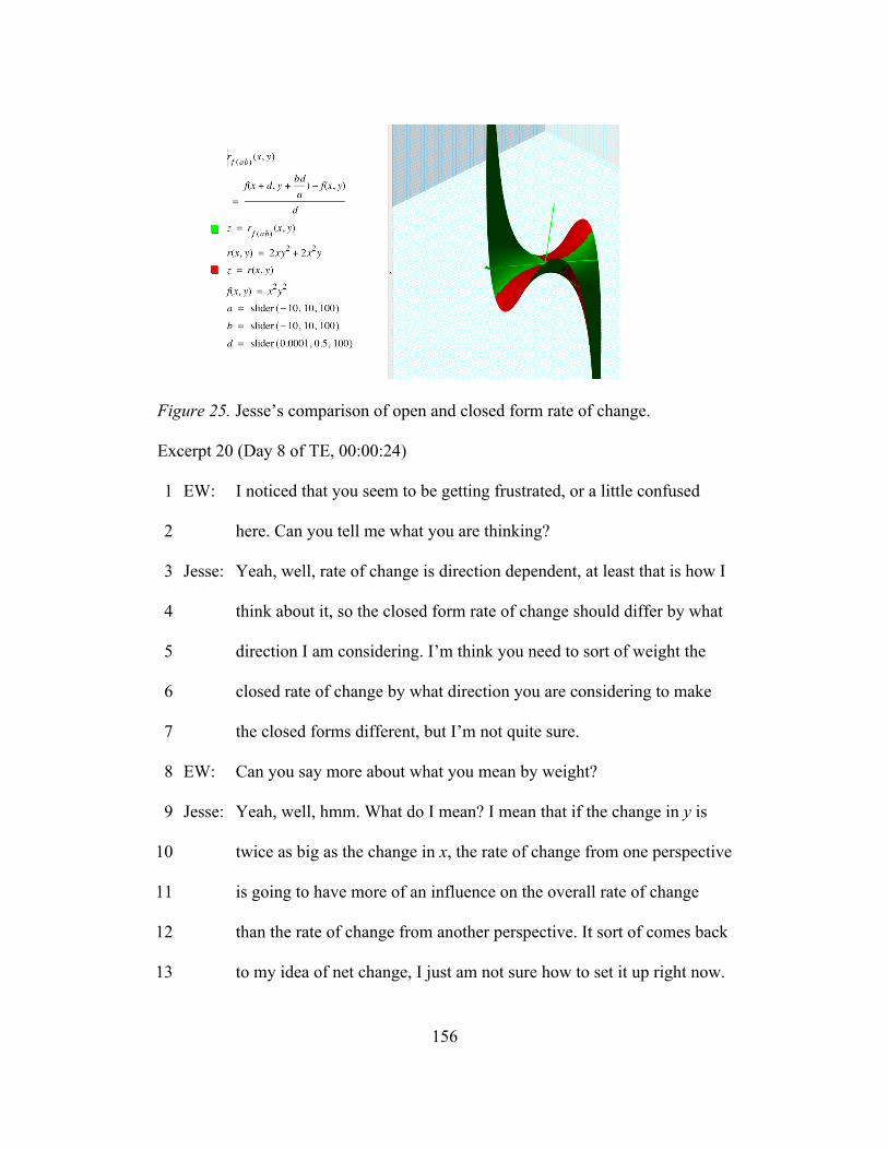
156
Figure 25. Jesse’s comparison of open and closed form rate of change.
Excerpt 20 (Day 8 of TE, 00:00:24)
EW: I noticed that you seem to be getting frustrated, or a little confused 1
here. Can you tell me what you are thinking? 2
Jesse: Yeah, well, rate of change is direction dependent, at least that is how I 3
think about it, so the closed form rate of change should differ by what 4
direction I am considering. I’m think you need to sort of weight the 5
closed rate of change by what direction you are considering to make 6
the closed forms different, but I’m not quite sure. 7
EW: Can you say more about what you mean by weight? 8
Jesse: Yeah, well, hmm. What do I mean? I mean that if the change in y is 9
twice as big as the change in x, the rate of change from one perspective 10
is going to have more of an influence on the overall rate of change 11
than the rate of change from another perspective. It sort of comes back 12
to my idea of net change, I just am not sure how to set it up right now. 13

157
Jesse’s was struggling to think about a “net” derivative (Excerpt 20, lines
12-13), but was imagining this net derivative as composed of the rate of change
from two directions. He appeared to be imagining the overall rate of change
(Excerpt 20, lines 10-11) as the result of adding multiple rates of change, each
weighted by some influence factor that depended on the relationship between the
change in x and the change in y. I believed that Jesse was dancing around the idea
of total derivative, but based on my model of his thinking, a great deal more
support was required to develop a meaningful and coherent notion of path
dependent and independent derivatives.
Figure 26. Jesse’s prediction of a closed form rate of change for f(x,y).
Part II Conclusions
My model for Jesse’s understanding of rate of change evolved based on
gaining insight into his understanding of open form rate of change, his meaning
for constant rate of change, and his understanding of a calculus triangle as a
measure of a rate of change function. My model of his thinking also developed
from specific instructional supports such as using his way of thinking about
perspectives in visualizing functions of two variables to help him imagine
calculus triangles in each perspective.

158
Meaning for rate of change.
Jesse described the meaning of average rate of change of quantity A with
respect to quantity B as the constant rate of change of quantity A with respect to
quantity B required to produce the same change in quantity A over the equivalent
change in quantity B. I believe that his use of open form and closed form rate of
change allowed him to think about average rate of change as the dependent
quantity in the open form rate of change function. He imagined open form rate of
change (which implicitly was associated with average rate of change) as an
approximation to closed form rate of change (which he associated with an exact,
or instantaneous rate of change) for small values of the change in the independent
quantity.
Understanding of the calculus triangle.
Jesse’s use of a fixed value of h to compare differences in the dependent
quantity suggested that he was already implicitly using the calculus triangle. Jesse
began to think about the calculus triangle and open form rate of change as
equivalent ideas. For example, he noted that the calculus triangle was a graphical
representation of the quantities in the open form rate of change function. At the
same time, his use of a calculus triangle allowed him to think about three ideas
that were not apparent in his initial open form rate of change function. First, he
imagined the calculus triangle sliding through the domain of the function, which
resulted in tracking the value of the rate of change. Second, he imagined that an
infinite number of very small calculus triangles existed in the domain of the
159
function. Third, he was able to illustrate the idea of fixing h as a parameter value
and by making h small, the value returned by comparing the lengths of the legs of
the calculus triangle would approach the “exact” rate of change of the function as
a point.
Extending rate of change to two variables.
Jesse’s focus on rate of change using calculus triangles became clear when
he initially grappled with the meaning of the rate of change at a point in space.
His initial attempts to describe rate of change in space combined his
understanding of average rate of change, his notion of calculus triangles, and his
way of thinking about visualizing two variable functions from different
perspectives.
He used his understanding of perspective and calculus triangles to imagine
perspective dependent calculus triangles that would measure the rate of change of
z with respect to x, or z with respect to y, and attempted to combine these values
to define a rate of change at a point in space. I used directional rate of change as a
way to help him resolve his imagery of simultaneous calculus triangles in the z-x
and z-y perspective with independent changes in the dependent quantities x and y.
By thinking about a calculus triangle in a direction in space, Jesse was able to
define an open form rate of change function, which he believed measured the
average rate of change of a dependent variable with respect to two independent
variables.

160
Total derivative.
Jesse’s development of “overall rate of change” suggested that when
thinking about rate of change at a point in space, he was dancing around the idea
of thinking about the path to the point (x, y). I believe that it would have required
numerous extra sessions to problematize the issue of directional and total
derivative to think about directional derivative as path dependent. However, I do
anticipate that given these extra sessions, Jesse’s ways of thinking could support
thinking about the function f at (x,y) as differentiable when all the directional
derivatives at (x,y) lie in a plane, but the time constraints of this teaching
experiment did not allow for this development to take place.
Chapter Summary
In this chapter, I have described the evolution of my inferences for Jesse’s
ways of thinking about two-variable functions and their rates of change. While I
examined the ways of thinking about visualizing functions separately from
thinking about rate of change, Jesse’s ways of thinking about these ideas were
developing simultaneously, as in the case of thinking about z-x, z-y and x-y
perspectives. I demonstrated the development of inferences for his thinking by
describing my hypotheses, a description of key excerpts, and my reflections from
each teaching experiment session. In doing so, I described expert shape thinking,
perspective thinking, and calculus triangles as key understandings for Jesse’s
ways of thinking.

!
! !161
Chapter 6
JORI’S THINKING
In this chapter, I describe Jori’s thinking. Jori was a student enrolled in
first semester calculus, as she participated in a teaching experiment focused on
functions of two variables and their rates of change. I describe her association of a
graph with a malleable object and her attempt to associate a set of symbols with a
memorized image of the graph from her calculator. I argue that she focused on
features of a graph as an object in space, which constrained her in imagining a
function’s graph as an emergent representation of quantities having covaried.
Lastly, I describe how Jori’s focus on rate of change as a calculation associated
with the slant of a graph constrained her from thinking about rate of change as a
comparison between changes.
Background Jori “was not a fan of mathematics”, which she attributed to difficulty in
high school mathematics and science courses. She described herself as a high-
achieving student “overall, just not in mathematics”. She attributed her success or
failure to sources outside of her control, such as the teacher, the workload of the
class, or the general idea that mathematics was confusing. She noted her
experiences in her calculus course were frustrating because she was required to
think about the meaning of an answer, but her intent when solving a problem was
to come up with the correct calculation. She believed she was not really “doing
mathematics” because she was pressed to describe how she was thinking about
new ideas rather than how to do calculations.
!
! !162
Jori scored near the mean on the calculus readiness exam administered at
the beginning of the semester. She was enrolled in first semester calculus when
she participated in the teaching experiment, and in that course, she had average to
below average scores on exams. She often “punted” away clarifying questions
from the instructor or other classmates. For example, in class she described the
rate of change as represented by a straight line, a number of her group members
suggested she meant constant rate of change. She described that she saw no
difference between what she said and what they said, and dismissed their appeals.
Initial Inferences about Jori’s Ways of Thinking I worked with Jori five times during tutoring in the two weeks before the
teaching experiment. When she defined a function, she described a set of values
for quantities in the problem and attempted to define a function that fit only a
static set of values. For example, when she was working on defining the distance
of the bottom of a ladder away from a wall as a function of time given that the
ladder started out three feet from the wall and was sliding at 2 feet/sec, she
created a set of points (1,2), (2,4), and described them as time, and how far the
ladder was away from the wall. She then plotted these points, and tried to define a
function whose graph would fit through all of the points she had generated. Her
approach suggested that she read problems by focusing on the numbers in the
problem statement. Her focus on constructing graphs by connecting points
suggested she was not attending to the graph as a representation of the
relationship between quantities’ values as they vary. Because of these behaviors, I
!
! !163
believed that Jori thought about graphs of one-variable functions as wire-like
objects in a plane.
Jori’s teaching experiment began after Jesse’s was completed, and used
the same tasks. However, I adjusted the sequence of the tasks. I moved the rate of
change tasks later in the teaching experiment so as to provide a more cohesive
focus for my generation and evaluation of hypotheses. As a result, day-to-day the
focus of our discussions was on material covered at most three days before. The
breakdown of tasks and the day on which they took place is in Table 18.
Table 18 !Task Sequence for Jori’s Teaching Experiment.
Task Description Date (Day)
Homer: Correspondence Points and Graphs 4/5/2011 (1) (10am)
Homer: Moving Cities and Varying Animation 4/5/2011 (2) (5pm)
Generating Graphs of f (x) = x3,g(x) = 2x 4/7/2011 (3)
Generating Graph of h(x) = x3 ! 2x 4/7/2011 (3)
Anticipating Behavior of m(x) = a(x3 ! 2x) 4/7/2011 (3) 4/9/2011 (4)
Treating a as a Third Axis 4/9/2011 (4)
Box Problem: Box Construction and Treating Parameters as Variable
4/12/2011 (5)
Generalized Functions: Construction and Interpretation of Graphs
4/14/2011 (6)
Car A – Car B: Interpreting Meaning of the Graph 4/16/2011 (7)
Car A – Car B: Measuring Rate of Change Using the Graph 4/17/2011 (8)

!
! !164
Box Problem: Measuring the Rate of Change at a Point in Space
4/20/2011 (9) 4/23/2011 (10)
Drivercost Problem: Parameters as Variables and Rate of Change 4/25/2011 (11)
Generalized Rate of Change Function and Direction
4/25/2011 (11) 4/27/2011 (12)
Working with Strange Functions (More than 2 variables) 4/29/2011 (12)
Part I: Jori’s Ways of Thinking about Two-Variable Functions
Part I of this chapter focuses on the development of a model for Jori’s
thinking about the behavior of two-variable functions. This part of the teaching
experiment comprised Days 1 to 6.
Days 1 and 2 – The Homer Activity
Based on my initial assessment of Jori’s thinking, I anticipated that the
Homer situation would present two perturbations to her thinking. First, the
construction and representation of quantities’ magnitudes on the axes would be
problematic because she was accustomed to focusing on numbers. Second,
imagining a correspondence point that tracked these two quantities’ magnitudes
simultaneously would not fit with her general conception of a graph as a path that
connects a discrete set of points. I anticipated that her conception of a graph
would rely on the graph “looking like” the situation. In the Homer situation, this
could be a road and two paths emanating from Homer.
On Day 1, Jori mimicked Homer’s motion when asked to track Homer’s
distance from Springfield and Shelbyville. She noted that she focused on Homer’s
motion, not his distance from the cities, and was unsure why his distance from

!
! !165
each city was important. The following excerpt occurred after my discussion with
her about how to focus on Homer’s distance from each city as she tried
representing Homer’s distance from each city using a vertical and horizontal “bar”
in Geometer’s Sketchpad.
Excerpt 21 (Day 1 of TE, 00:00:24)
Jori: Well, when I am trying to pay attention to both of his distances at the "!
same time, it is really hard. I understand how to represent both #!
distances, Shelbyville on the horizontal and Springfield on the vertical, $!
but I’m having trouble trying to track both of them. %!
EW: Can you tell me what you are having the most trouble with? &!
Jori: I guess I’m not quite sure, but when I was paying attention to each '!
distance individually, I could just make sure my finger was moving (!
like Homer was moving on the road, kind of keeping the same speed )!
and tracking his distance, but now my fingers can’t both imitate *!
Homer’s motion at the same time, it’s just frustrating, I’m not sure, "+!
uh… ""!
EW: Are you trying to imitate Homer’s movement, or trying to track the "#!
distance from each city? "$!
Jori: I guess I am trying to do both of them. I kind of lose track of the "%!
distances when I am trying to keep up with Homer’s motion. [As the "&!
animation moves, she appears to focus on the distances exclusively]. "'!
Uh, well, it is a lot harder, but I feel like I am being more accurate "(!
when I am not trying to keep up with Homer’s motion at the same time. ")!

!
! !166
EW: Okay, so what are you trying to pay attention to now? [as Homer is "*!
moving on road in the animation] #+!
Jori: Well, it seemed like I want two distances, so I have to find Homer’s #"!
distance from the two cities at the same time. At first I thought I would ##!
have to imitate his motion, but the distances make more sense. They #$!
aren’t the same.#%!
Once she focused on Homer’s distance from each city as a quantity, Jori
was able to imagine each distance varying individually, but found it problematic
to track both of the distances simultaneously (Excerpt 21, lines 4, 6-7). She
attributed this difficulty to the importance of mimicking Homer’s motion (Excerpt
21, lines 7-11). Even as she attempted to track a distance, and imagined those
distances having values simultaneously (Excerpt 21, lines 21-24), Jori was
imitating the motion in the animation (Excerpt 21, lines 14-15). I anticipated, in
the moment, that her inattention to quantities would foster a way of thinking about
a correspondence point as a feature of the Homer animation rather than a
representation of the quantities in it.
After introducing the notion of a correspondence point, I asked Jori to tell
me what she understood about the behavior of the point. Her responses suggested
to me that she felt “in control” of the correspondence point at every instant. By
this, I mean she felt the point could be manipulated without affecting Homer’s
location on the road. The following excerpt occurred after discussion about the
correspondence point as a representation of Homer’s distance from each city.

!
! !167
Excerpt 22 (Day 1 of TE, 00:00:45)
EW: You were struggling with the correspondence point idea earlier, but "!
pretty quickly picked up imitating its behavior. #!
Jori: Yeah, once I realized it did not need to imitate Homer, it was easier. $!
You asked me to think about it leaving a trail behind [sketches the trail %!
she anticipates]. I think this [pointing to Figure 27], would be what it &!
left behind. It tracks where the correspondence point has been, and sort '!
of shares some things that look like the road and the cities’ locations. (!
EW: So what do you pay attention to decide if the path is accurate? )!
Jori: Well, it has to make sense with the situation, so it has to imitate some *!
of Homer’s motion no matter what. A graph tracks a situation, so "+!
sometimes it will look like that situation. ""!
EW: Well, let’s look at the trail that the sketch produces. [Reveals computer "#!
sketch, Figure 28]. What do you think? "$!
Jori: It sort of opens upward, like I thought. The rest is weird, but I could "%!
probably account for it if I was more exact in my measurements. "&!
Figure 27. Jori’s anticipated tracing out of the correspondence point.

!
! !168
Figure 28. Computer generated graph of Homer’s distance from two cities.
Jori indicated that the correspondence point was not representative of
Homer’s motion, but its path would be related to Homer’s location on the road.
This concept of mimicking fit with her concept of a graph as “looking like” the
situation it represented (Excerpt 22, lines 9-11). Jori appeared to be convinced
that the correspondence point would rely on the features (e.g. road) of the
situation. She may have been trying to express quantities created by measuring
aspects of those features, but her thinking was very muddled. Her description of
the graph “opening upward” and her inability to describe why it opened upward
(Excerpt 22, line 15) was evidence that she may have been thinking about a graph
as an object in space.
Jori’s focus on Homer’s movement along the road had two consequences.
First, she focused on recreating features of the animation in her graph. Second,
her focus on Homer’s movement likely led to her inattention to the Homer’s
distance from the two cities as quantities. Her description of the correspondence
point as recreating Homer’s motion suggested that she was not attending to the
values represented on the axes. Thus, after the morning teaching session (Day 1) I

!
! !169
believed that she was not thinking about the correspondence point as a
representation of two quantities’ values. I thought she focused completely in the
quadrants. For example, when describing her graph as opening upward (Excerpt
22, line 14) she was focused on describing the shape she saw, rather than thinking
about how the shape was related to the quantities in the Homer context.
At the beginning of the afternoon session (Day 2), I tested these
hypotheses by asking Jori 1) to anticipate how the graph would change if
Shelbyville and Springfield were moved and 2) to describe the location of the
cities given a graph that represented Homer’s distance from each city
simultaneously. I anticipated that if she focused only on the shape of the graph,
she would imagine that a transformation of the quantities in the Homer animation
as unrelated to the graph.
I exchanged the location of Springfield and Shelbyville in the animation in
the first minutes of Day 2. I intended to understand how Jori would think about
the effect of this exchange on Homer’s distance from each city in the animation.
Jori said that the graph would not change, because “all of the objects are in the
same place, the names are just different in this case” (Figure 29). Her response
indicated that she was focused on the location of objects in the animation. I
believed, in the moment, she thought because the graph was accurate an exchange
of the cities did not affect the graph. This indicated to me that she was not focused
on what each axis represented, which constrained her from imagining the graph as
a representation of quantities having covaried.

!
! !170
Figure 29. Jori’s anticipated graph after I exchanged the positions of the two
cities.
Excerpt 22 was the first indication of what I called a focus on the
quadrants. When Jori imagined graphing a function or interpreting an already
constructed graph, she appeared to think about the features of the object in space
as just features. The features were not emergent or imbued with quantitative
properties. As a result, Jori was unable to the functional relationships that these
“features” represented because they were not representations of quantities. For
example, Jori believed the graph would remain invariant under an exchange of
cities. She appeared to associate a single graph with the Homer situation, and
because the shape of the graph was not the output of covariational reasoning, this
graph did not need to transform even though the cities locations were exchanged.
I then gave Jori an already-generated graph (Figure 30) and asked her to
say where the cities might have been located to generate this graph, in anticipation
that if she could not imagine the graph’s shape as a result of the distances having
covaried, she would describe the graph as a roadmap of how Homer moved in the
animation. Our discussion is given in Excerpt 23.

!
! !171
Excerpt 23 (Day 2 of TE, 00:00:12)
EW: Okay, so we are going to kind of work in reverse here. Given this "!
graph (Figure 30), could you tell me where the cities might be located #!
in the animation? $!
Jori: Okay, I’m going to assume everything works the same way. The first %!
thing I notice is that the lines of the graph hit the axes here, so that &!
might mean Homer turns around at those points, maybe turns around '!
from the cities? Well, but at the same time, the graph I’m seeing here (!
opens up and is kind of square like, not smooth like the other ones, so, )!
umm, I would guess that because there is straightness, well, he’s *!
maybe traveling at a constant rate to or from each one of them? "+!
EW: What do you mean by them? ""!
Jori: The cities. The linearity of the graph means he’s going at a constant "#!
speed, I think, or that he is traveling in a straight-line path. "$!
Figure 30. The graph Jori was given to determine the location of the cities.
Jori’s responses indicated that she had engaged in novice shape thinking.
It seemed that the associated the image of a straight line with “constant speed”
and that a sharp corner meant “turn around”. Because she was focused on
meanings implied to her by the graph’s shape she was not attending to the axes or

!
! !172
how distances from cities were represented on the axes and reflected in the
correspondence point’s position. This association is supported by her description
of graphs not as a relationship between quantities’ values, but as conveying
meanings unrelated to the situation (e.g., “straight means constant speed”, Excerpt
23, lines 12-13).
In my reflection on Days 1 and 2, I noted that Jori’s lack of quantitative
reasoning differentiated my model of her thinking from Jesse’s. Jori appeared to
associate the graph with an object that had physical features, but those features
were non-quantitative. I anticipated that Jori’s lack of attention to how graphs as
an emergent representation of covariation and her focus on the graphs as shapes
would lead to her associating a surface in space with an object, where that object
was independent of the quantities I intended her to use to generate the surface.
Day 3 - The Difference Function ! !
I had not anticipated the degree to which Jori would focus on the shape of
graphs and struggle with imagining their construction. I believed it would be very
difficult to observe a major shift in her thinking about the graphs of functions
because of her insistence on focusing on the graph as an object in space with
properties independent of the function that generated it. Given this issue and
Jori’s time constraints, I believed it would be powerful to characterize how her
ways of thinking constrained her in thinking about two-variable functions. Thus, I
moved forward in the activity sequence. !
I anticipated that generating a difference function where the algebraic
forms of functions were given would reveal her association of the graph as an

!
! !173
object situated in the quadrants, independent of quantities that generated it. As
such, I believed that she would imagine the difference function as a physical
combination of the graphs and their features. The following excerpt occurred at
the beginning of Day 3, in which we discussed how to think about generating the
graphs of the functions f (x) = x3 and g(x) = 2x .
Excerpt 24 (Day 3 of TE, 00:00:05)
EW: If we are generating the functions x3 and 2x , how are you thinking? "!
Jori: Well, I am trying to think to when I have used my graphing calculator. #!
I know 2x is a straight line because it has a constant slope, but x3 is $!
difficult because I can’t remember how the function looks. I think it is %!
sort of wavy. &!
EW: How do you approach generating a new function if you haven’t seen it '!
before? (!
Jori: Generally, umm, I just use a graphing calculator, then, and then and try )!
to memorize the shape of the graph, kind of the contours I see. Then I *!
can figure out what other similar algebraic functions look like, and see "+!
if they imitate the same shape. ""!
EW: So how would you go about looking at the cubic term? Or should I say, "#!
how does a calculator know how to graph that function? "$!
Jori: Well, I remember the wave sort of, but I’d have to ugh, well, plug in a "%!
bunch of numbers and then connect the points as best as I can. I’d "&!
probably try to connect a wave, because that’s what I remember. "'!

!
! !174
EW: Okay, well, remember our discussion about the correspondence point, "(!
how would that come into play here? ")!
Jori: I’m not sure, I’m not sure how to track the things I need to track."*!
Jori “generated” graphs by trying to recall their shape from a graphing
calculator (Excerpt 24, line 2). She appeared to memorize a graph’s shape and
contours and compared those shapes to general classes of algebraic functions
defined by their shape (Excerpt 24, lines 10-11). Thus, I believed to Jori, an
equivalence class, or family, of functions was completely reliant on the shape of
the graph, independent of imagining that graph as an emergent representation of
two quantities having covaried. It appeared to me, in the moment, that Jori
imagined the calculator running a process in which it plugged in a bunch of
numbers, then “connected a wave” that went through each point (Excerpt 24, line
16). I believed, while working with her in Day 3, that she was trying to connect
points in space rather than points in space created by quantities’ values
represented on the axes.
I asked her how she would think about generating a difference function
composed of the two functions she had just graphed using Graphing Calculator. I
anticipated that she would focus on 1) generating the function’s graph by
attempting to imagine what it would “look like” and plot points and try to guess
as to how the points were connected, and 2) combining the shape of the two
graphs into a graph that shared features of each individual graph.

!
! !175
Excerpt 25 (Day 3 of TE, 00:00:24)
EW: So, given your graphs of the two functions, let’s try to create a new "!
function, which is the difference between these two, x3 ! 2x . #!
Jori: Okay, oh, great. Ugh, I’m having trouble doing this because I’m not $!
sure about x3 , but I graphed it in GC, so I know what it looks like. If I %!
can graph both functions together, I might have a better idea. &!
EW: Can you say any more? What might you do with the two graphs? '!
Jori: You said a difference function, right? Yeah, okay, well, if it is a (!
difference, I’d imagine it goes through the middle of the space between )!
the two functions [draws linear function crossing through open space *!
between two functions, see Figure 31]. "+!
EW: I’d like you to use GC to compare the graph you generated. ""!
Jori: Okay, umm, [graphs difference function], wow. I didn’t expect those "#!
humps to be there, they are taller than both of the functions. I figured a "$!
difference would mean the functions sort of meet in the middle, but "%!
GC says the humps on the function actually get bigger. "&!
EW: Okay, I just want to finish on this question, if we defined a new "'!
function, where we multiply a parameter by x3 ! 2x , how would the "(!
function behave? ")!
Jori: In class, the y values would only change, so that would make the "*!
humps taller and skinnier I think, if the parameter gets bigger like you #+!
seem to be asking. #"!

!
! !176
Figure 31. Jori’s anticipated graph of the difference function.
Jori focused on what each graph “looked like” as if she were describing an
object in space. She wanted to have both graphs displayed simultaneously to see
what a function composed of the two might look like (Excerpt 25, lines 4-5). She
believed the difference function would lie between the graphs of the two original
functions (Excerpt 25, lines 8-9). Her way of thinking about the “difference
function” appeared to rely on splitting the difference between objects, which I
referred to as “meeting in the middle” (Excerpt 25, lines 14-15). I allowed her to
graph the function (Excerpt 25, lines 12-13), and she was surprised by the “humps”
in the function’s graph because the graph was “taller” than either of the original
functions (Excerpt 25, lines 12-14). This excerpt was also the first case where she
began distinguishing between what she thought, and what she believed GC
(Graphing Calculator), to be telling her (Excerpt 25, lines 16-17). She attributed
the difference in what she anticipated and what GC produced as the result of an
error in Graphing Calculator.
Even though she attributed an error to Graphing Calculator, she relied on
it to depict the behavior of a function novel to her. I believed that even if she
possessed a graphing calculator to graph a function, her understanding of how it
was generated could be thought of as “calculator magic”, she was not even sure
the calculator was not full of errors. I thought her need for the graphing calculator

!
! !177
to see the “shape” of an object perpetuated itself. She could not imagine graphs of
novel functions because she did not have a general scheme for how a graph was
generated.
Day 4 - Sweeping Out a One-Variable Function I predicted that thinking about sweeping out a function’s graph to generate
a surface in space would not fit with Jori’s association with a graph as
independent of quantitative relationships. I predicted that if given a surface in
space, her inattention to the axes would lead her to focus on features of the
surface, much like a topographical map. At the same time, I anticipated that
developing the idea of perspective would support Jori in imagining the surface of
the graph in space from multiple perspectives, but that she would focus on the
shape of the surface or the appearance of the graph from multiple perspectives. To
evaluate these hypotheses, Day 4 focused on imagining a surface being swept out
in space.
At the beginning of Day 4, Jori described the effect of a on
h(x) = a( f (x)! g(x)) “vertically affecting the difference function we had before.
The a only affects the output value, because the x stays the same, the a has no
effect on the x is what I am trying to say”.
I asked Jori to think about a as the distance in front of or in back of the
laptop screen. Jori appeared to visualize this effect of a as the graph sliding along
another axis. In the following excerpt, I asked her to describe the tracing out of
the function’s graph to produce a surface in space.

!
! !178
Excerpt 26 (Day 4 of TE, 00:00:13)
EW: In the Homer activity, we talked about tracing out a function from a "!
point. In this case, I want you to imagine we are sweeping out a #!
function along a third axis, which is given by a, and represents the $!
distance in front of or in back of the laptop screen. %!
Jori: Do you want me to use this strip of paper? It might help. [interviewer &!
nods approval]. Okay, well, as a changes, the humps of this function '!
are going to get larger as a gets more negative and more positive, kind (!
of creating tunnels that open [Draws Figure 32]. This piece of paper is )!
kind of like my starting graph, and then adjusts when a changes. *!
EW: Okay, could you say a little more, where are these humps coming from, "+!
what makes them appear? ""!
Jori: The tracing out you said, described, it’s what happens when you "#!
follow and track where the strip of paper has been. "$!
Figure 32. Jori’s sketch of the effect of a on the difference function.
Jori responses indicated to me that she was imagining the effect of a on
the shape of the function’s graph (Excerpt 26, line 6-7). Her description of
“tunnels that open up”, suggested she imagined a surface being produced as the
function varied with values of a (Excerpt 26, lines 7-9). I believed she was

!
! !179
thinking about the piece of paper moving through space, staying perpendicular to
the a axis, and thinking that the graph changed within the piece of paper, which
created a surface. Then, the “tunnels” and “humps” became larger as the paper’s
distance from the x-y plane increased.
Excerpt 27 (Day 4 of TE, 00:00:34)
EW: So when you are considering the sweeping out we just talked about, "!
what are you visualizing? #!
Jori: I’m kind of imagining watching it happen from the side, if I watched it, $!
umm, directly [pause], I don’t think I could see 3-D because I %!
wouldn’t have much depth. &!
EW: Can you describe again how this function is generated? '!
Jori: Well, I treat the output like the upward axis, and a kind of like another (!
variable, but like a parameter at the same time. Then I change the )!
parameter and track the function, where it leaves a trail behind, here *!
sort of tunnelish looking. In 3-D, I think it is normal say up is “z”. "+!
EW: Okay, I’d like to think about this as the z-x view, where we are ""!
considering z as a function of x, and treating y like a parameter value "#!
to imagine it sweeping out. This might seem strange, but given this, "$!
what might a z-y view be? "%!
Jori: Well, offhand I’d treat x like a parameter, and y like a variable, kind of "&!
watching the function tracing out happen from a different viewpoint. I "'!
still think it would create the same shape overall, same features, same "(!
ups and downs and curves. ")!

!
! !180
EW: What would be the generating function in the z-y perspective? "*!
Jori: It would be a parameter times a variable, but I have no idea what the #+!
graph would look like. I’m not sure how I would check it in GC, but it #"!
looks like a straight function from z-y [Sketches Figure 33].##!
Jori’s description of watching the sweeping out occur from the “side”
suggested she was comfortable thinking with depth. Jori described the sweeping
out of a function by thinking about a as “like another variable”, but like a
parameter at the same time (Excerpt 27, lines 7-9). Her description suggested that
she was thinking about a as a variable, and she found it useful to think of a as a
variable, even though it could be used like a parameter. Her characterization of
the z-y perspective revealed that she viewed perspective as a way to view a
surface in space (Excerpt 27, lines 15-17), but had difficulty imagining how that
surface was constructed (Excerpt 27, lines 21-22).
Figure 33. Jori’s depiction of viewing two perspectives.
I believed Jori had accommodated her ways of thinking about functions of
one variable to fit with a surface in space. When she was able to think about a
sweeping out occurring, her description of the resulting surface in space focused
on its physical features (i.e. ups, downs and curves). This was much like Jesse’s
descriptions, but I believe that she associated the ups, downs and curves as the

!
! !181
result of sweeping out, but what was swept out was a wire independent of
covariational reasoning. This does not suggest that her thinking was “bad”, but
does support that even as she and Jesse used the same words to describe the
surface, only Jesse imagined that surface imbued with quantities’ values. I used
the box problem context on Day 5 to evaluate these hypotheses.
Between Day 4 and 5 - Jori’s Reflections on Parameter
I believed it was critical to establish Jori’s distinction between a parameter
and a variable. I asked her to write a short reflection on this topic between Days 4
and 5. Prior to Day 5, I asked Jori to describe her use of “parameter” and
“variable”. Jori described a parameter as “a letter that represents a number, like
we talked about in class, kind of like a variable except you are in control of it and
can change its value, where a variable is something you are not really in control of,
our instructor said it’s like representing a whole bunch of values at the same time.
I think they are the same because a parameter and variable represent numbers, but
are different because one represents a whole bunch of numbers and values while
the other only represents one”.
Her response indicated to me that she imagined a variable representing a
continuum of values, while a parameter represented a single value, which she
could specify. It appeared that for her to imagine the sweeping out occurring, she
needed to imagine that she was changing a parameter value. I anticipated that
treating a like a variable meant she imagined the sweeping out having already
occurred over a continuum of values, each of which could have been represented
as a parameter.
!
! !182
Day 5 - The Box Problem Entering Day 5, I believed Jori was focused on the graph as an object
situated in the quadrants, which along with having difficulty imagining a function
being swept out, restricted her from thinking about the function that graph
represented. I believed that these ways of thinking applied to both her
understanding of one-variable functions, and the sweeping out of a one-variable
function to a surface in space. I intended to gain insight into how she constructed
an image of the volume of the box as a function of the cutout length, and how that
image would constrain her conception of the graph of the volume function. I was
also interested in understanding her distinction between a variable and a
parameter, and how that supported her in visualizing a surface in space. In the
following excerpt, I asked Jori to describe the volume of the box as a function of
the cutout length.
Excerpt 28 (Day 5 of TE, 00:00:04)
EW: Suppose you are a box designer, and you must program a computer to "!
determine the volume of an open box, which has no top to it. This #!
open box is created from making cutouts from a rectangular sheet of $!
paper. Jori, could you tell me how you would think about making such %!
a box, as well as how to represent the volume of the box? &!
Jori: I finally got an easy one! The function would be volume equals length '!
minus two x times width minus two x times x, where x [creates Figure (!
34] is the cutout you make from the sheet of paper, right? )!

!
! !183
EW: That seemed pretty easy for you, what made it that way? *!
Jori: Well, the box to have uniform height means the cutouts have to be the "+!
same because the cutouts are the same as the height. Then from length ""!
and width, you take away two cutout lengths to make the box, then fit "#!
that into the formula for volume. "$!
EW: Good! What do you imagine would happen to the volume if the cutout "%!
started increasing from a small value to a larger one? "&!
Jori: Not sure, I would test it out, but probably the box volume keeps "'!
getting smaller the whole time because there is more cutout. Can I put "(!
this function in graphing calculator? That’s messed up, well, I guess I ")!
was wrong. The volume gets bigger for a while, then smaller. "*!
EW: When you say for a while, what do you mean? #+!
Jori: Umm, well, look, the volume goes up, then it goes down again, so it is #"!
getting bigger for a while, but I was mostly right. ##!
Figure 34. Jori’s image of the construction of the box.
Jori’s described the volume of the box (Excerpt 28, lines 6-8) as a function
of the cutout length. Her anticipation of how the sheet of paper would fold up into
a box allowed her to distinguish between the length and width of the box and the

!
! !184
length and width of the original paper (Excerpt 28, lines 10-13). Her
understanding that the box height would be uniform required all cutouts to be the
same length, and the measure of the length of the cutout was equivalent to the
height of the box (Excerpt 28, lines 10-11).
Jori also imagined the cutouts becoming larger, which made the length and
width of the box smaller, but she did not account for the increase in box height
resulting from the increasing cutout length (Excerpt 28, lines 18-19). When she
inputted the function into graphing calculator, she was surprised that the graph
showed the volume going up, and down again (Excerpt 28, line 21), but
immediately punted away this issue, saying she was mostly right (Excerpt 28, line
22). As Jori followed the path of the graph, she focused on the “hump” that the
function produced without explaining how the hump fit with the function she
constructed.
Two minutes after the discussion in Excerpt 28, Jori described how the
graph of the function was really hard to think about because it was a third degree
polynomial once the function was expanded. She indicated that once she had a
general idea of what a third degree term does to a function’s graph, she might be
able to “have a decent idea of what the graph looks like and why”. Her response
suggests to me now that if she knew the shape of a graph and she could imagine
how the shape was affected by changing the parameter, she could operate like
Jesse in generating a surface. It was also plausible that her reliance on a graph’s
shape revealed itself when she had difficulty graphing a function with which she
was not familiar.

!
! !185
In the following excerpt, I asked Jori to imagine that the base of the box
was represented by a parameter value. I anticipated that based on her initial
description of volume going up then down, she would continue to associate the
graph with an object independent of quantities represented by the function. I
intended to gain insight into how creating a “strange” situation (where a is a
function of x) would affect her interpretation and construction of the graph.
Excerpt 29 (Day 5 of TE, 00:00:29)
EW: When you talked last time, you had also described the formula for "!
volume as base multiplied by height? #!
Jori: Yeah, well, base comes from length times width. $!
EW: Okay, let’s suppose we treat the base like a parameter value. %!
Jori: Okay, so you want me to do that sweeping out with the function again? &!
Again, I think the function is only going to stretch vertically when I '!
increase the parameter value, and shrink vertically when I decrease it, (!
so the path it would leave behind would be an open tunnel, which )!
might get bigger or narrower, I'm not sure, I’d have to do the math to *!
test out which one it really is. "+!
EW: Why don’t you test it out in GC, and talk me through it? ""!
Jori: Okay, well, let me make this a parameter, okay, Weird! I have no idea "#!
what’s going on there, but I’ll look in a second. If I do this as a two "$!
variable function, I just replace a with y, and define f(x,y), and I kind "%!
of think there must be a tunnel [looking at Figure 35]."&!

!
! !186
Figure 35. The tunnel Jori viewed in the Box problem graph.
I inferred that Jori was thinking about a parameter value as a third axis,
along which the sweeping out of the one-variable function took place. Her
description of the effect of the parameter (Excerpt 29, lines 7-8), and of the shape
of the path left behind (Excerpt 29, lines 8-9), suggested to me that Jori was using
facets of both expert and novice shape thinking. She could associate the surface in
space with the effect of the parameter value on that surface (expert), while
describing features of the graph without explicit attention to the quantitative
relationship that it represented (novice). Her actions also suggested that she was
thinking about graphing f (x, y) = xy , not f (x, y) = x*g(x) where y = g(x) . She
appeared to be using a parameter as a way to think about generating the surface of
a function. Jori provided evidence for this claim when she replaced a with y
(Excerpt 29, line 14), and in defining and graphing f(x,y), anticipated a “tunnel”
(Excerpt 29, line 15) appearing without describing a tracing out of a function in a
plane that could create the tunnel.
Jori’s responses suggested to me that her distinction between parameter
and variable went further than “numbers”. She used a parameter as a way to
!
! !187
imagine sliding a one-variable function in a plane along a third axis, where the
parameter values represented specific snapshots of that function. Imagining the
snapshots being displayed simultaneously for every value on the third axis fit with
Jori’s use of a variable because she anticipated a variable representing all possible
parameter values, creating a surface without going through the process of tracing
out.
Excerpt 29 suggested to me that novice and expert shape thinking needed
to account for how a student generates a graph and interprets a graph. I now
believe that characterizing shape thinking an association the student has with a
graph accomplishes this purpose. Jori was able to describe how the surface in
space was generated, but when she focused on interpreting that same surface, she
was focused on the graph as an object with physical properties. In both cases, she
displayed some sophisticated methods of constructing the surface in space.
However, she appeared to associate the surface with an object situated in the
quadrants. An expert shape thinker, I believed then, should be able to imagine a
graph being generated, and given a graph already generated, all the while
imagining that graph as an emergent representation of two or more quantities’
covariation.
My hypotheses about Jori’s novice shape thinking and her distinction
between parameter and variable were generated from this excerpt as well as my
reflections from numerous teaching episodes. In Excerpt 30, I intended to gain
insight into Jori’s thinking about graphs of two-variable functions, as well as how
she would interpret and use the notion of perspective. I intended to understand if

!
! !188
Jori’s use of perspective could support her in imagining a surface in space and its
generating functions in the context of the Box problem (Figure 36).
!
!Figure 36. The Box problem graph’s generating functions.
Excerpt 30 (Day 5 of TE, 00:00:55)
EW: We talked earlier about thinking about the z-x and z-y perspectives for "!
functions. Can we do the same thing here? [Reveals Figure 37] #!
Jori: Sure, but it’s more like volume-cutout and volume-length perspectives $!
because we know what the things are we are measuring. %!
EW: You mentioned earlier the perspectives help you look at the function in &!
different ways? '!
Jori: Yeah, well, for volume-cutout, I just treat length like a parameter, and (!
volume-base, treat cutout like a parameter. I figure, I can do this and )!
have cutout-base view too where volume is a parameter. But I can’t *!
visualize the exact sweeping out until I graph it. I mean, I know how it "+!

!
! !189
gets created, but I can’t see it until I look at it in graphing calculator, ""!
either on the computer or in an actual calculator. [Looks at Figure 37]. "#!
EW: What about the process you just described? Does that help you think "$!
about how the function was created? "%!
Jori: No, not really, because I really need to get an idea of what the surface "&!
looks like, its’ kind of been like looking at maps for me, and imagining "'!
I’m looking at it from the East or the West. I sort of have to see the "(!
whole before I can see each view and part. Sometimes the parameter ")!
thing helps, but it’s also hard to visualize."*!
Figure 37. Graph shown to Jori in discussion about perpsectives.
Jori said she could imagine “how it gets created”, referring to the surface
in space (Excerpt 30, line 11). I believed she was saying “how” while imagining
the process of generating a surface in space by sweeping out a function in the
plane. Her description of volume-cutout and volume-length perspectives (Excerpt
30, lines 3-4) suggested she imagined parameterizing paper length and cutout
length, respectively to produce the sweeping out. However, Jori’s description of a
looking at a map (Excerpt 30, line 16) suggested that even as she imagined a
perspective as a way to generate a function’s surface, she was quick to fall back

!
! !190
on shapes in the quadrants. It seems that in both cases her thinking could have
been non-quantitative. Even as she was describing the sweeping out, the surface
that resulted was not necessarily imbued with quantities’ values.
Day 6 - Functions in Space
To evaluate the viability of my hypotheses about Jori’s focus on a graph as
an object in the quadrants, I asked her to do two things. First, given the algebraic
form of a two-variable function, construct its graph in space. Second, given the
graph of an unknown two-variable function in space, describe a possible algebraic
form for the function. I used the first activity because I anticipated that thinking
about generating a surface given a two-variable function was not possible without
using a graphing calculator. I anticipated she would rely on identifying the shape
of the object without imagining the surface being generated from multiple
perspectives. I used the second activity because I believed that interpreting a
graph without the given algebraic form of the function, and asking her to create
the generating function could not be done without her attending to the axes. I
began the session by asking her to describe the behavior of the function
f (x, y) = x2y2 , without being able to graph the function in Graphing Calculator.
Excerpt 31 (Day 6 of TE, 00:00:04)
EW: We’ve been mostly, uh, working with applied situations, so I want to "!
work with something you might see more often for functions. Let’s say #!
we have a function x squared times y squared. Can you take me $!
through how you would think about this function? %!
Jori: It has squares in it, which make me think parabolas right away. &!
!
! !191
EW: Where do these parabolas come from? '!
Jori: The algebra says they are there I think. If you have a square, (!
something is probably a parabola. )!
EW: Could you describe how you might think about generating the function *!
from each perspective, before we get to graphing it? "+!
Jori: I said, that’s too hard, I’m not sure. ""!
EW: Okay, from z-x, you said y is like a parameter. If that is the case, what "#!
kind of function do we have? "$!
Jori: a times x squared? Yeah, so if a is one, or wait, any value, it’s a "%!
parabola. Oh, same for the other perspective! They sort of combine "&!
then, right? "'!
EW: What do you anticipate? "(!
Jori: I need to look overhead somehow, but without graphing the function, ")!
that seems impossible. "*!
EW: You mentioned earlier treating the output like a parameter, would that #+!
help? #"!
Jori: Maybe, then it would be the x-y view, yeah! Then I could tell how the ##!
two other views sort of work together.#$!
Jori’s description of f(x,y) as involving parabolas because “it has squares
in it” (Excerpt 31, line 5), and her description of the parabolas coming from the
“algebra” (Excerpt 31, line 7), suggested to me that she was attempting to recall a
shape that she associated with a particular set of symbols. Even in her description
of the z-x and z-y views, she focused on connecting a symbolic representation she

!
! !192
had associated with a particular shape (Excerpt 31, line 14). Her description of the
perspectives combining (Excerpt 31, line 15), and using the x-y view to see how
the other views combine (Excerpt 31, lines 22-23), indicated to me, in the moment,
that she was describing an already generated graph of a two-variable function,
rather than imagining its construction from multiple perspectives.
During a break in Day 6, I anticipated it would be problematic for Jori to
analyze a graph of a two-variable function to determine the algebraic form of the
generating function. I believed that unless she was able to identify shapes that
readily fit with specific classes of functions she already knew, the situation would
be untenable for her. For example, if she noted a feature of the graph that looked
linear, she would conjecture that the function definition must include a linear term.
Excerpt 32 (Day 6 of TE, 00:00:37)
EW: For this last one, I’m going to do a little changeup. I’m giving you this "!
graph [the graph was of f (x, y) = x2y ], but not telling you the function. #!
Could you think about how to determine what the function is? $!
Jori: Ugh, no, this is like reverse thinking like integration, and I’m bad at %!
that too. &!
EW: Just give it your best shot. '!
Jori: Alright, well, from this side it (Figure 35) looks like a line, and the (!
other it looks like a curve, maybe a parabola? I would guess the )!
equation has a curve and a parabola in it then, right? *!
EW: As you are looking at this graph, what is your strategy? "+!
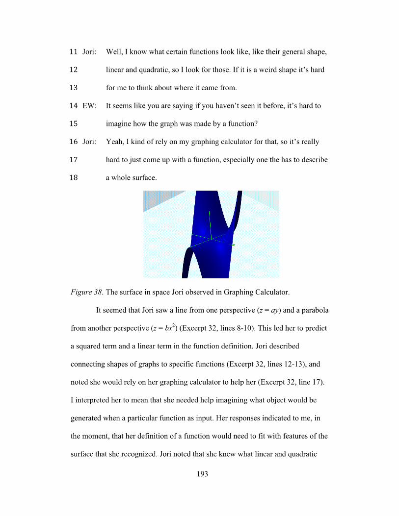
!
! !193
Jori: Well, I know what certain functions look like, like their general shape, ""!
linear and quadratic, so I look for those. If it is a weird shape it’s hard "#!
for me to think about where it came from. "$!
EW: It seems like you are saying if you haven’t seen it before, it’s hard to "%!
imagine how the graph was made by a function? "&!
Jori: Yeah, I kind of rely on my graphing calculator for that, so it’s really "'!
hard to just come up with a function, especially one the has to describe "(!
a whole surface.")!
Figure 38. The surface in space Jori observed in Graphing Calculator.
It seemed that Jori saw a line from one perspective (z = ay) and a parabola
from another perspective (z = bx2) (Excerpt 32, lines 8-10). This led her to predict
a squared term and a linear term in the function definition. Jori described
connecting shapes of graphs to specific functions (Excerpt 32, lines 12-13), and
noted she would rely on her graphing calculator to help her (Excerpt 32, line 17).
I interpreted her to mean that she needed help imagining what object would be
generated when a particular function as input. Her responses indicated to me, in
the moment, that her definition of a function would need to fit with features of the
surface that she recognized. Jori noted that she knew what linear and quadratic

!
! !194
functions looked like, but that almost any other shape was hard for her to connect
to a specific type of function. Her description of the graph as an object in this
context supported my hypothesis that she thought about a function was just a set
of symbols associated with a particular shape situated in the quadrants.
Part I Conclusions
My inferences about Jori’s ways of thinking occurred in the context of
already having conducted a teaching experiment with Jesse, which affected my
instructional supports and the ways in which I wanted to engender ways of
thinking about two-variable functions. My analyses revealed a number of
constructs that became aspects of the more general concept of novice shape
thinking.
Novice shape thinking.
Novice shape thinking occurs when the student associates a graph with an
object in space, where that object is not an emergent construction. For example,
Jori could imagine the process of how a shape was constructed in space, but often
did not think about the resulting surface as the result of covariation. In my
reflections, I wrote that Jori appeared to associate a graph with a malleable object.
By malleable, I mean that she appeared to think about a wire (one-variable) or
topographic map (two-variable) when she looked at a graph. A key component of
her focus on a graph as a malleable object was her focus on the quadrants in the
plane and in space. When Jori imagined graphing a function or interpreting an
already constructed function, she was focused on the features of the object in
space, without reference or attention to the functional relationships that these

!
! !195
“features” represented. As a result, the graph was not an emergent construction
that represented quantities having covaried.
The graphing calculator Jori referenced using a graphing calculator thirty-nine times, each of
which was in the context of “having the graphing calculator do that” for her. The
majority of the time she did not know how to use a graphing calculator when she
offloaded a particular task to it. The graphing calculator was a way to “punt”
away her difficulties. For example, when I asked her how she would use a
graphing calculator to help her visualize a two-variable function, she initially said
she did not quite know how to program it, she just knew what she wanted it to do
overall. This supports the notion that Jori could describe the general sweeping out
process to create a surface in space, but sometimes imagined that process
independently of imagining quantities covarying. I believed that she saw the
graphing calculator as a tool to solve everything she did not understand. In
particular, when she did not know what the graph looked like given a particular
function, she could use the calculator to the graph an object in space.
Part II: Jori’s Ways of Thinking about Rate of Change The second part of this chapter focuses on Jori’s ways of thinking about
rate of change, and how those ways of thinking supported and constrained her in
making sense of the rate of change of two-variable functions. My observations of
Jori’s class work, homework, and interactions during tutoring hours suggested to
me that she equated rate of change with calculating slope, often independent of
thinking about a relationship between two quantities. She described rate of change

!
! !196
as the same “idea” as a slope because the calculations were identical. She also
described the calculation of rate of change as the calculation of “something about
a straight line”. Her responses suggested that the meaning of an idea was
equivalent to its calculation. Thus, she interpreted the value of rate of change as a
feature of a straight line. I anticipated that her way of thinking about slope
constrained her from thinking about rate of change as a function. For example,
Jori described open form rate of change as slope and “just a fancy method that
could be replaced by using a rule”. The outline of days and particular activities
discussed in Part II are in Table 19.
Table 19
Jori’s Rate of Change Task Sequence.
Task Description Date (Day)
Car A – Car B: Interpreting Meaning of the Graph
Constant and Average Speed Activity 4/16/2011 (7)
Car A – Car B: Measuring Rate of Change Using the Graph 4/17/2011 (8)
Box Problem: Measuring the Rate of Change at a Point in Space
4/20/2011 (9) 4/23/2011 (10)
Parameters as Variables and Rate of Change 4/25/2011 (11)
Generalized Rate of Change Function and Direction
4/25/2011 (11) 4/27/2011 (12)
Day 7 - Car A-Car B Activity
I intended to use the Car A – Car B activity to understand how Jori’s
meanings for slope and rate of change were connected to ideas from her calculus
course, such as open form rate of change and calculus triangles. I anticipated that
she would find these ideas equivalent to the method for calculating them because
!
! !197
of her focus on calculations. In the following excerpt, I asked Jori to interpret the
meaning of the graphs in Car A – Car B crossing after one hour.
Excerpt 33 (Day 7 of TE, 00:00:10)
EW: In the Car A- Car B situation I just described, and here is the graph "!
again, could you tell me what information the graph is providing? #!
Jori: The graph seems to give a location of the car as it travels, oh wait, a $!
speed of the car as a travels over time. It looks like the cars meet each %!
other after one hour has elapsed because the graphs cross. &!
EW: What does it mean for the graphs to cross in this context? '!
Jori: It means, um, they are meeting each other, wait, no, they have the (!
same speed, I’m not sure if they are crossing each other’s path at that )!
time. *!
EW: Could you describe Car A’s rate of change? "+!
Jori: Well, you can tell the rate of change, which we know here is ""!
acceleration because we already have speed, is like the slope. The "#!
slope is getting less and less [points to point on graph after 0.2 hrs, 0.5 "$!
hrs], so the car is decelerating. "%!
EW: When you say the slope is getting less and less, what do you mean? "&!
Jori: The straight line along the curve would be getting more horizontal. "'!
EW: What does that mean about the car’s acceleration? "(!
Jori: It means it is getting less, the slope is getting less, calculating it as a ")!
change in speed over a change in time. I think more horizontal means "*!
less, yeah [Constructs Figure 39]. #+!
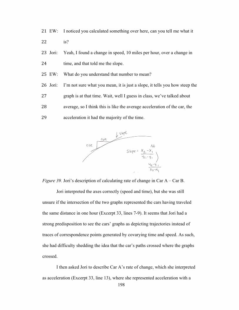
!
! !198
EW: I noticed you calculated something over here, can you tell me what it #"!
is? ##!
Jori: Yeah, I found a change in speed, 10 miles per hour, over a change in #$!
time, and that told me the slope. #%!
EW: What do you understand that number to mean? #&!
Jori: I’m not sure what you mean, it is just a slope, it tells you how steep the #'!
graph is at that time. Wait, well I guess in class, we’ve talked about #(!
average, so I think this is like the average acceleration of the car, the #)!
acceleration it had the majority of the time. #*!
Figure 39. Jori’s description of calculating rate of change in Car A – Car B.
Jori interpreted the axes correctly (speed and time), but she was still
unsure if the intersection of the two graphs represented the cars having traveled
the same distance in one hour (Excerpt 33, lines 7-9). It seems that Jori had a
strong predisposition to see the cars’ graphs as depicting trajectories instead of
traces of correspondence points generated by covarying time and speed. As such,
she had difficulty shedding the idea that the car’s paths crossed where the graphs
crossed.
I then asked Jori to describe Car A’s rate of change, which she interpreted
as acceleration (Excerpt 33, line 13), where she represented acceleration with a

!
! !199
slope (Excerpt 33, line 12). Her gestures indicated that she was imagining slope at
two points, after 0.2 hours and after 0.5 hours. Her description of the slope
“getting less and less” (Excerpt 33, line 13) because of a “straight line along the
curve getting more horizontal” (Excerpt 33, lines 18-20) suggested she was
focused on a feature of the graph (a straight line). She indicated that she thought
about the value of slope as a measure of steepness of a graph (Excerpt 33, lines
26-27), which she recalled should be associated with the word “average”, or a
property that a quantity possessed most of the time (Excerpt 33, line 29).
I believed, in the moment, that Jori was thinking about rate of change as
an equivalent to slope, where slope meant the “slant” of a graph. Thus, I believed
rate of change was simply a feature of an object in her thinking. Her description
of the rate of change as the acceleration the car had the “majority of the time”
(Excerpt 33, line 29) suggested to me that she was not thinking about measuring a
ratio of changes in two quantities. Given Jori’s lack of focus on rate of change as
a comparison of changes, I inserted an extra activity into Day 7 that allowed me to
better understand her way of thinking about steepness. I intended to draw her
focus to the ratio of changes in two quantities.
Day 7 - Constant and Average Speed Activity
I posed the following situation to Jori: Suppose you have your car on
cruise control, and as you pass mile marker 110, a truck passes you. Assume that
you keep your cruise control set to the same speed, and you pass the truck at mile
marker 117, six minutes later. I asked her to describe everything she could about
the situation.

!
! !200
Excerpt 34 (Day 7 of TE, 00:00:35)
EW: What can you tell me about what is going on in this situation? "!
Jori: Umm, well, you basically are driving and you are going at the same #!
speed the whole time, and the truck must speed up and slow down $!
again because he passes you, and then you pass him about seven miles %!
later. &!
EW: Could you say more about what it means to travel at the same speed '!
the whole time? (!
Jori: Well, for any amount of distance, if you go that distance again it will )!
take the same amount of time. *!
EW: Okay, if it takes you 55 seconds to travel one mile, how long would it "+!
take to travel 1.25 miles? ""!
Jori: Well, I need to do some multiplication, but, it would just be 55 "#!
seconds plus a fourth of 55 seconds. "$!
EW: Interesting, how did you get to that point? "%!
Jori: Well, he always takes 55 seconds to go a mile, so a quarter mile will "&!
take a fourth of that because he is on a constant speed. "'!
EW: And what about how far he would go in 123 seconds? "(!
Jori: Well, divide 55 into 123, that many miles.")!
Her way of thinking about constant speed always taking the same amount
of time to travel a particular distance (Excerpt 34, lines 8-9) supported her in
thinking about how long it would take to travel some fraction of one mile
(Excerpt 34, lines 12-13). Her understanding of constant speed can be described

!
! !201
as if one travels x miles in y seconds, then in some fraction (a/b) of x miles, one
travels (a/b) of y seconds, and vice versa. I anticipated that thinking about
constant rate of change in this way would allow Jori to think about average rate of
change as a comparison of changes. In the next excerpt, I asked Jori to think about
the average speed of the car and the truck from the example I posed to her, and
describe how she would measure average speed.
Excerpt 35 (Day 7 of TE, 00:00:58)
EW: So, what did you come up with in regard to the average speed of the "!
car and the truck? #!
Jori: Well, at first I figured the average speed of the car is the speed he goes $!
most of the time, which in this case is all the time, but then I %!
remembered talking in class about average speed, and I know &!
somehow I need to bring in a change in distance and time, which I '!
guess doesn’t work with speed most of the time. (!
EW: How do you see it not fitting? )!
Jori: Well, so, I was thinking if you just have a change in distance and *!
change in time, the truck could have been going all sorts of crazy "+!
speeds between the miles, but his average speed is the same as yours ""!
because of the same distance same time, and he wasn’t going the same "#!
speed as you most of the time, err, or didn’t have to be I think. "$!
EW: So, I want to say this, and have you explain what you hear me saying. "%!
!
! !202
Average speed over a given time interval is like the constant speed "&!
another object would need to travel to go the same distance in the "'!
same amount of time. Think for a minute, and tell me what you heard. "(!
Jori: Well, that makes sense, because all you know is the two changes, time ")!
and distance, and for your car going the same speed the whole time, "*!
the changes were the same as the truck. My most of the time thing is #+!
more conventional, not the mathy use of average I guess. #"!
EW: Okay, and if you sketched a graph of the car’s distance with respect to ##!
time and the truck’s distance with respect to time between the mile #$!
markers, what do you anticipate? #%!
Jori: Well, one would be curvy, the truck’s, and the other would be straight. #&!
EW: When you say curvy and straight, what are you paying attention to? #'!
Jori: The car goes the same distance every minute, for example, so kind of #(!
like slope, you go up and over the same each time, so it’s straight, but #)!
the truck doesn’t need to do that, as along as he starts and ends at the #*!
same points. $+!
Jori initially said average speed was the speed traveled “most of the time”
(Excerpt 35, lines 3-5), but recalled a discussion from her calculus course about
average speed resulting from changes in distance and time (Excerpt 35, lines 6-7).
She described the car and truck as having the same average speed as the total
changes in distance and time were equivalent for each vehicle (Excerpt 35, lines
9-13). She agreed with my description of average speed as a constant speed
because “all you know is the two changes, time and distance” (Excerpt 35, lines

!
! !203
18-21), which she believed were the same for the car and truck. She described her
definition of average speed as “conventional”, and mine as “mathy”. It seems that
in earlier phases of this task, Jori’s “conventional” meaning is the one upon which
she relied.
I believed, in the moment, that it was critical for Jori to represent average
and constant rate of change. Her description of the graph’s of the car and trucks’
distances with respect to time as “curvy” and “straight” (Excerpt 35, line 25)
suggested she was thinking in terms of shapes. Her description of the straight line
as generated by going up and over the same each time (Excerpt 35, line 28), but I
believed she was focusing on the slope without imagining measuring the rate of
change of the car’s distance with respect to time. I asked Jori to construct a
function that would measure the “exact” speed at which the car was traveling, in
anticipation that the issue of exact speed would allow us to talk about average rate
of change over very small intervals of input.
Excerpt 36 (Day 7 of TE, 00:01:10)
Jori: So, if I wanted to make that function to get exact speed, I know I "!
would have to look at a really small change in time, like 1 second, or #!
maybe even less than that, and how far I went in that small time. $!
EW: Okay, so how would you create a function that would do that for you? %!
Jori: Well, let’s see, oh, like slope? Umm, this is just like the open form &!
from class! '!
EW: Say more. (!

!
! !204
Jori: Well, I just have f(x+h) – f(x) on top, and h on the bottom, and I have )!
always thought of it like slope, except with function notation. *!
EW: Okay, how would that be related to exact speed? "+!
Jori: You could just make h really small, that’s like making time small, then ""!
the top tells you how far you went, and then you divide. "#!
EW: Does that tell me an exact speed? "$!
Jori: Almost exact, I guess. For .0001, it’s pretty much exact. "%!
EW: But, is it exact? "&!
Jori: No, I guess. It’s not exact, it’s just an average, oh constant speed, but "'!
it’s pretty much exact, we can’t really see that small of a change, it’s "(!
too quick.")!
Jori’s thought about exact speed as a change in distance over a very small
change in time required to travel that distance (Excerpt 36, lines 1-3). She
assumed that exact speed could be measured by making the change in time small
enough. She recognized this situation as appropriate for “open form from class”
(Excerpt 36, lines 5-6), which indicated that she could see open form rate of
change comparing the changes in two quantities, although this is not the meaning
that came first to mind for her. However, Jori also appeared to think about open
form as slope (Excerpt 36, lines 8-9). Jori anticipated that to measure exact speed,
h (change in time) must be small. She suggested if h was .0001, the speed would
be “pretty much” exact (Excerpt 36, line 14). Jori eventually said that she was
thinking about open form rate of change as equivalent to an average, and in turn,
constant rate of change (Excerpt 36, lines 16-17).
!
! !205
At the conclusion of Day 7, I suspected that Jori’s preferred meaning for
rate of change was steepness of the line segment between two points. When
interpreting rate of change in the context of a graph, Jori rarely referred to
measuring the change in one quantity in terms of the other. It appeared her
primary way of thinking about slope was a degree of slant between two points.
Day 8 - Jori’s Reflection on Rate of Change
I used Day 8 to gain insight into how Jori was thinking about average rate
of change, open form, and calculus triangles. I believed that it was important for
me to understand how she related those representations in order to understand
how she would think about rate of change in space.
Excerpt 37 (Day 8 of TE, 00:00:12)
EW: So, after the last session in which we talked about the meaning of "!
average and constant speed, what do you understand now that you #!
weren’t so comfortable with before? $!
Jori: I guess, umm, I see how average speed is like a second trip sort of idea %!
that produces a same change in distance during a same change in time, &!
and it can happen over really small intervals to get more exact. '!
EW: How is that related to your overall understanding of rate of change? (!
Jori: It’s interesting, because I see it is kind of related, it is almost like open )!
form rate of change, but not like closed form. It also seems like the *!
calculus triangle thing we work with in class, but I’m not sure exactly "+!
how. I know in open form and the calculus triangle, like the trip we ""!
talked about, you can make the input very small, a slider value of h, to "#!

!
! !206
calculate a pretty accurate rate of change. You can sort of pull out the "$!
calculus triangle on a graph to do this when you need a rate of change "%!
value. "&!
EW: You also mentioned open form? "'!
Jori: Yeah, open form is kind of like the calculation behind the calculus "(!
triangle, it gives you, like an average speed, or rate of another trip in ")!
the trip example you and I talked about earlier. This is all different "*!
from closed form, which is like an exact rate of change, a perfect one #+!
that does not involve an h. So basically, thinking graphically, it tells #"!
you the degree of slant of the graph, which is related to speed, I think. ##!
Jori used a “second trip” to think about average speed, which led to her
focus on changes in distance and in time (Excerpt 37, lines 4-5). She also
indicated rate of change could be thought of over “really small intervals” (Excerpt
37, line 6), which suggested she was thinking about average rate of change as an
approximation. I believed, in the moment, that she was thinking about open form
as the calculation behind the calculus triangle (Excerpt 37, line 17-18). However,
I believed that the meaning she attributed to what I called rate of change had little
to do with rate. By this, I mean that she was able to use open form rate of change
and a calculus triangle, but was unsure how to interpret the result of that
calculation. She indicated she saw the measurement as “speed” (line 22), but was
unsure as to how it related to speed.
Jori seemed to be making shifts in the moment, such as developing
meaning for average speed and its measurement, but was also falling back on her

!
! !207
tendency to calculate without interpretation. I anticipated that Jori would focus on
drawing similarities between the calculation of rate of change in the plane and
rate of change in space. Thus, I anticipated asking her to describe the meaning of
rate of change in space would provide insight into what she believed the
calculations of rate of change represented. Based on her descriptions, I believed
she would describe rate of change in space as a degree of slant at a point.
Day 9 - Sweeping Out a One-Variable Function
Day 9 focused on rate of change in space. I anticipated that Jori would
think about rate of change at a point in space as a degree of slant between two
points, but representing the correct changes would produce host of issues. I
believed she would be able to visualize a calculus triangle in the z-x and z-y
perspectives, but I anticipated her focus on calculations and not on meaning of
rate of change would make it difficult to see a direction in space as important. I
began our discussion by asking Jori about the sweeping out of the function h(x) =
a(f(x)-g(x)).
Excerpt 38 (Day 9 of TE, 00:00:06)
EW: In the function where we talked about thinking with depth and "!
sweeping out a new surface, how would you approach talking about #!
rate of change? What might be the same or different from just a one $!
variable function? %!
Jori: Well, man, this is pretty weird to think about. It’s like z is changing &!
with x and y, so it can’t just be a simple description. My first guess, '!
though I have no idea if I am right, is that, hmm, I don’t know. (!

!
! !208
EW: Assume we had a rate of change for functions of two-variables, and it )!
returned a number like 3.45. How would you interpret the meaning of *!
the 3.45? "+!
Jori: I’d say it was an average change, constant rate of change, but I’m not ""!
sure of what with respect to what, especially when x and y are both "#!
involved. It might be like a combination of the rates from the z-x and "$!
z-y perspectives we just talked about, like two rates in different "%!
directions that you need to combine I think. Then you can make it like "&!
one variable thing. I’d probably just sum the two rates of change, one "'!
for z-x and one for z-y."(!
Jori’s description indicated she was imagining z changing with respect to x,
and z changing with respect to y (Excerpt 38, lines 5-6). Because I anticipated she
was thinking about rate of change as a combination of degrees of slant, I asked
her to interpret a rate of change value. She described the value as an average,
constant change (Excerpt 38, line 11). However, she was unsure of how to
describe z changing with respect to x and y (Excerpt 38, line 13). She proposed
combining (Excerpt 38, line 15) the perspectives’ rates of change because she
wanted the calculation to be similar to what she was comfortable with in functions
of one-variable. After this excerpt, she made two conjectures about rate of change
in space (Figure 40). I asked her to solidify her conjectures and discuss the
strengths and weaknesses she saw in each rate of change function.
I anticipated she was focused on combining the rate of change in each
direction to account for being in space. I believed that the purpose of her

!
! !209
combination was to make the structure of the two-variable rate of change function
similar to the two dimensional case.
Figure 40. Jori’s conjectures about a two-variable rate of change function.
Excerpt 39 (Day 9 of TE, 00:00:37)
EW: Let’s look at the conjectures you developed. You mentioned looking at "!
rates of change in each perspective. Would it help to think about #!
calculus triangles in each perspective? $!
Jori: Sure, umm, I think that’s what I am doing in my first conjecture here, I %!
kind of have a z-x and z-y calculus triangle, and I am adding them &!
together. I sort of want to take the calculus triangles and make a '!
calculus wedge of cheese (Figure 41), like a three-dimensional object (!
made up of the two triangles, but I don’t know how that might work. )!
EW: Alright, can you say more about where your calculus triangles are in *!
your first conjecture, because you said you had them? "+!
Jori: Yeah, well, I took the rate of change for a function of x and a function ""!
of y and basically combined them. "#!
EW: What do you anticipate that your first rate of change function will do? "$!
Jori: It takes a rate of change for x and y, and combines them to make a total "%!
rate of change. "&!
EW: Alright, could you say more about your second conjecture? "'!

!
! !210
Jori: Yep, this one was harder, but basically I was thinking, there is a two "(!
variable function, so we have to use both variables, so I figured you ")!
have to add h to each x and y, so you get a change on top that does "*!
what the first conjecture did, but in a shorter calculation, then you get #+!
the change on the bottom, which comes from adding h two times. #"!
EW: Okay, in your second conjecture I noticed you are using h for the two ##!
views that you are adding together. Are they the same h? #$!
Jori: Yep. These are the same, but, mmm, I’d guess they don’t need to be #%!
because you can pick any value you want for each of them, huh? I #&!
guess for the one calculus triangle in each perspective, the little bit you #'!
add could be whatever you wanted.#(!
Jori’s description of imagining a single calculus triangle in the z-x and z-y
perspectives (Excerpt 39, lines 4-6), and combining those triangles to make a
calculus wedge (Excerpt 39, line 7, see Figure 40) suggested to me she was
attempting to combine features of two one-variable functions from the z-x and z-y
perspectives. She attempted to mimic the structure of the one-variable open form
rate of change function in both conjectures, and noted the difference between the
two was primarily in whether the function V should include x and y
simultaneously. Jori’s second conjecture did allowed her to consider that the
change in x and y need not be equivalent (Excerpt 39, lines 24-27).

!
! !211
Figure 41. Jori’s drawing of the calculus cheese.
In my reflection after Day 9, I surmised that Jori thought about rate of
change as a feature of a graph that could be combined with other features by
simple calculations. Jori’s model for understanding rate of change at a point in
space was to consider how to perform an operation on the rate of change value
from the z-x and z-y perspective. Essentially, she imagined a slope from each
perspective to produce a total slope at a point in space. Her focus on making the
two-variable rate of change function structurally equivalent to the one-variable
rate of change function created many issues when she attempted to combine two
rates of change. The calculus cheese appeared to be an ad hoc way of accounting
for rate of change in two directions. It seems that once she constructed the
calculus cheese, she believed it was plausible to add the two rates of change as it
fit with her need to “combine”.
Day 10 - The Box Problem
On Day 10, I intended to evaluate the viability of describing Jori’s
thinking about rate of change of a two-variable function as the result of
combining the degree of slant between two points, each obtained using the z-x
and z-y perspective. I also intended to affect this way of thinking by asking her to
construct calculus triangles from each perspective using function notation. By
!
! !212
asking her to construct the calculus triangle in the z-x and z-y perspectives, I
intended Jori would think about the comparison of the “legs” of the triangles as
representing partial rates of change. I also anticipated that Jori’s novice shape
thinking and understanding of graphs as objects was foundational to her notion of
slope and rate of change and would make any major shifts in her thinking
momentary.
Excerpt 40 (Day 10 of TE, 00:00:07)
EW: You’ve had a little while to look over the candidate rate of change "!
models that you came up with before, how are you thinking about #!
them now? $!
Jori: I realized that what I was doing before would not quite work, the %!
calculus triangle from each perspective would have to include a &!
consistent y in the z-x view or consistent x in the z-y view, or I mean, I '!
have to account for that variable. So I would use f(x+h,y) – f(x,y) for (!
z-x and f(x,y+h) for the z-y view numerator [Sketches Figure 42]. I )!
hadn’t accounted for it being two variables before. *!
EW: Okay, great, that’s really insightful. So could you say more about what "+!
you mean by consistent? ""!
Jori: Well, by consistent, you have to keep the variable steady, so you can "#!
look at a normal calculus triangle, so I could give y a value of three, "$!
then be looking in the z-x perspective, like here [points to Figure 42]. "%!
EW: Also, remember when we talked at the end of the last session about "&!
adding a little bit to x and a little bit to y? Could you recap? "'!
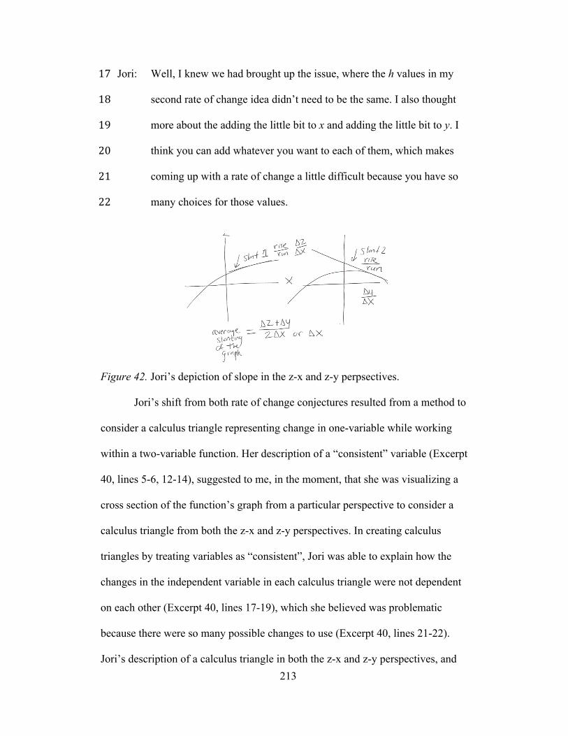
!
! !213
Jori: Well, I knew we had brought up the issue, where the h values in my "(!
second rate of change idea didn’t need to be the same. I also thought ")!
more about the adding the little bit to x and adding the little bit to y. I "*!
think you can add whatever you want to each of them, which makes #+!
coming up with a rate of change a little difficult because you have so #"!
many choices for those values.##!
Figure 42. Jori’s depiction of slope in the z-x and z-y perpsectives.
Jori’s shift from both rate of change conjectures resulted from a method to
consider a calculus triangle representing change in one-variable while working
within a two-variable function. Her description of a “consistent” variable (Excerpt
40, lines 5-6, 12-14), suggested to me, in the moment, that she was visualizing a
cross section of the function’s graph from a particular perspective to consider a
calculus triangle from both the z-x and z-y perspectives. In creating calculus
triangles by treating variables as “consistent”, Jori was able to explain how the
changes in the independent variable in each calculus triangle were not dependent
on each other (Excerpt 40, lines 17-19), which she believed was problematic
because there were so many possible changes to use (Excerpt 40, lines 21-22).
Jori’s description of a calculus triangle in both the z-x and z-y perspectives, and

!
! !214
her problematizing of the changes in x and y, suggested that she could understand
the need for a direction in space. Day 10 ended due to an unexpected class
conflict for Jori, and we picked up with discussion on Day 11.
Excerpt 41 (Day 11 of TE, 00:00:03)
EW: You said earlier you could add a little bit to y and a little bit to x in the "!
rate of change function. What issues did that bring up? #!
Jori: Well, it seems like there’d be no way to get a consistent rate of change $!
if you are wildly picking those two values all the time, but like I said %!
before, I don’t see any way to deal with that. &!
EW: We’ve looked at these calculus triangles from the z-x and z-y '!
perspective, how could the x-y perspective help us? (!
Jori: I can see what overhead direction I’m looking? I don’t know… )!
EW: Sure, let’s build on that, suppose you are going in a direction where *!
the change in y is twice as large as the change in x. "+!
Jori: Well, that would follow this line [indicates a linear trend from a point ""!
in space] h2 would be twice as big as h1 then, I think. "#!
EW: What if you made one of them small, how does that affect the other? "$!
Jori: That makes it… oh! It makes it small too, like just by doing one thing "%!
you end up doing two. "&!
EW: Okay, so what would happen if you made one change small, how "'!
would that affect the other change? "(!
Jori: Well, it would get small slower because the one change will always be ")!
two times as much the other, but eventually it could be pretty small. "*!

!
! !215
EW: So how would this be related to the calculus triangles we were talking #+!
about earlier? What would be the same and what might be different? #"!
Jori: You are kind of bringing the triangles together, but not quite in a ##!
wedge, more like into a direction.#$!
When I suggested that Jori consider the x-y perspective y (lines 6-7), she
described an “overhead direction” (Excerpt 41, line 8). She used her fingers to
indicate many possible directions emanating from a point in space being viewed
from the x-y perspective. I described a direction where the change in y was twice
as large as the change in x (Excerpt 41, lines 9-10). Jori interpreted this as a
specific direction emanating from the point in the x-y plane, making h2 (the
change in y) twice as large as h1 (the change in x). Jori’s response to my question
about how h1 and h2 behaved when one of them became small (Excerpt 41, lines
13,16-17), suggested that she had an image of the changes in x and y becoming
small simultaneously (Excerpt 41, lines 14-15). Jori also imagined that fixing a
proportional relationship between the changes in x and y was similar to describing
a calculus triangle in a direction (Excerpt 41, lines 22-23).
I asked Jori to consider how she might adjust her two rate of change
conjectures in light of the discussions we had about rate of change in a direction
to understand. I anticipated that while Jori had problematized that rate of change
could have a direction, the focus on direction was less important to her than
abstracting the structure of the one-variable rate of change function.

!
! !216
Excerpt 42 (Day 11 of TE, 00:00:31)
Jori: Alrighty, well, going back to my conjectures, I like number 2, but I "!
need to specify an h1 and an h2 , but there is also the denominator #!
issue. $!
EW: What issues are you seeing? %!
Jori: I don’t think I can have both of them down there, because I just want &!
to make one of the two values small, the h-values. '!
EW: Well, what happens if you just make one of them small? (!
Jori: Oh yeah, then the other gets small as well, sort of by force. I think I )!
can just leave one of them in the denominator then, and put the *!
numerator in terms of h1 because I can define one change in terms of "+!
the other when I know the ratio of their changes, like a direction. ""!
EW: Okay, great, so if you have defined the function, let’s say you get an "#!
output from your function of 2.95. How would you interpret that "$!
number? "%!
Jori: Like it has sort of been all along, it is like the total slope or slant at that "&!
point, looking in a direction. "'!
EW: Could you imagine it as related to average or constant rate of change? "(!
Jori: Umm, well, slope is like a constant rate of change, so you found the ")!
constant rate of change of the graph."*!
Jori’s solution to the denominator issue was to include just one of the h
values. This decision was dependent on her imagining that as h1 decreased and
became small, h2 was forced (Excerpt 42, line 6) to become small as well. By
!
! !217
imagining that h1 depended on h2 , Jori was able to write h1 in terms of h2 by
using a direction. Even as she attempted to make the structure of the two-variable
rate of change function like the one-variable rate of change function, she was able
to problematize that change in space has a direction. Jori developed an accurate
rate of change function, but her description of the output of the function as
measuring a total slope or slant (Excerpt 42, line 15), suggested she saw the
function as a method of combining two partial rates of change, where each rate of
change was a slant between two points. However, it was not clear in what sense
she understood rates to be combined. She associated constant rate of change with
slope (Excerpt 42, line 18), but noted the output of the rate of change function
was the constant rate of change of the graph (Excerpt 42, line 19). Thus, while she
developed important ways of thinking about the open form rate of change
function, she thought about rate of change in a superficial way.
Part II Conclusions Jori developed sophisticated ways of thinking about how to calculate rate
of change, even as she had difficulty interpreting the meaning of rate. She
appeared to make inroads in thinking about the meaning of rate, but was
handicapped by having “graph is a shape” filter into her thinking. Even when she
was thinking about graph as a shape, and rate of change as a measure of a slope
on that shape, she made progress in thinking about rate of change in space.
Jori focused on the making the calculation of a two-variable rate of change
function structurally similar to the one-variable case. Her construction of the
calculus cheese was a way to illustrate her focus on combining rates of change in

!
! !218
the z-x and z-y plane. Once she determined she needed to “combine” rates of
change, and addition was the most viable operation to do so, she developed
conjectures about a two-variable, open form rate of change function. She
attempted to mimic the structure of the one-variable rate of change function in
performing this addition. Even as she focused on drawing structural similarity
between one and two-variable rate of change functions, she broached the two
changes problem in two-variable rate of change. She was able to accommodate
this problem without focusing on the meaning of rate of change at a point in space
because she recognized there were two rates. She eventually grappled with the
issues of imagining h1 and h2 varying in tandem from considering a direction in
the x-y plane, which allowed her to develop an accurate two-variable open form
rate of change function, her interpretation of the function’s output did not change.
She thought about the output of the rate of change function as a slope.
Chapter Summary
In this chapter, I illustrated how Jori’s attention to a graph as an object in
the quadrants, sometimes without reference to what the object represented, led me
to hypothesize, within the teaching experiment, that she used novice shape
thinking. I described how Jori’s understanding of graphs as shapes and attention
to slope and calculations affected the development of ways of thinking that I
intended to support in the teaching episodes. While she relied heavily on
calculations and focused on graphs as shapes in the quadrants, she did think with
some sophistication within the teaching episodes. However, her thinking often
gravitated back to shapes and slopes.

!
219
Chapter 7
BRIAN AND NEIL’S THINKING
This chapter describes Neil and Brian’s ways of thinking. Neil and Brian
were enrolled in the same calculus course as Jesse and Jori. They participated
together in this teaching experiment, which changed the one on one dynamic of
the previous teaching experiments. The modified dynamic allowed me to observe
their conversations and the ideas they developed in the course of those
conversations. Thus, the basis for the development of my models of their thinking
included conversations between Neil and Brian as well as their interactions with
me.
In this chapter, I describe the how Brian and Neil made the programming
of a correspondence point the central issue of the teaching experiment. They used
a correspondence point to think about generating graphs of one and two-variable
functions. They also used the idea of programming to think about how to generate
a rate of change function in one and two variables. I describe the development of
their use of a correspondence point, and argue that it provided coherence for their
ways of thinking about the functions tasks and rate of change tasks.
Background
Brian and Neil worked with each other throughout the semester in calculus,
and their facility at discussing ideas with each other while focusing on ways of
thinking contributed to their engagement with the teaching experiment tasks.
Neil was a computer science major, and described himself as passionate about
mathematics. He had taken advanced mathematics in high school and at
!
220
community college, but because he was returning to school after a break, had not
remembered a lot of the “rules and procedures” he needed in order to be
successful. He described his use of graphing calculators and technology as a way
to “remedy” the procedures he had forgotten. He felt that it was easy to unload the
calculations onto the technology. He looked forward to his calculus course
because of the heavy use of technology. Brian was a construction management
major who had returned to school that semester and chosen to take calculus
because he was interested in mathematics. He was typically a detached student
who was not interested in participating or making sense of ideas, but said his
experience in calculus that semester had fundamentally changed how he thought
about mathematics.
Initial Inferences about Ways of Thinking
I started interacting with Brian and Neil when I began the first teaching
experiment with Jesse, and met with them as a group six times prior to the
beginning of the teaching experiment. My observations and exploratory teaching
interviews with them took place until the end of Jori’s teaching experiment. As I
created initial inferences about their ways of their thinking, I found that I
interpreted what they were saying and doing through the lenses I was developing
in the ongoing teaching experiments.
Brian could think about a graph of a function as a shape, but with the
understanding that the shape moved in response to a transformation of the
relationship the function represented. For example, he described a quadratic
function as “tilting upward”. He described how the tilting was generated by the

!
221
output becoming so many times larger than the input as the rate of change
increased. Brian made little distinction between the graph of a rate of change
function and the graph of a “normal” function. He said, “you can think of any
graph of a function as a rate of change function, no matter what it is”.
Neil focused on properties of graphs, such as slant and openness. For
example, in describing an exponential function, he said the “graph goes up
quickly”, but could not differentiate its behavior from a quadratic function whose
graph was similar. I anticipated his attention to the graph as an object could
constrain him in imagining a generating point for functions of one variable and a
generating function for functions of two-variables. Neil also was able to quickly
calculate a rate of change given a function definition, but he interpreted the rate of
change as a slope, which was not always connected with how fast a quantity was
changing with respect to another. During my interactions with them, I noted that I
was using facets of expert and novice shape thinking. Thus, unlike with Jesse, the
idea that someone could use aspects of both types of reasoning was part of my
initial hypotheses about their thinking.
Part I: Brian and Neil’s Ways of Thinking about One and Two-Variable
Functions
The teaching experiment began after my reflections on Jori’s teaching
experiment were completed. The sequence of activities followed the same outline
as my teaching experiment with Jori, but the timeline was compressed due to time
constraints of Neil’s summer work. As a result, the sessions were longer, but the
same activities were covered (Table 20). Note the first two activities took place on

!
222
the same day (5/5/2011), but were 5 hours apart. I conducted analyses between
the sessions, and thus, counted them as distinct days.
Table 20 !Task Sequence for Brian and Neil’s Teaching Experiment.
Task Description Date (Day)
Homer: Correspondence Points and Graphs 5/5/2011 (1) (10am)
Homer: Moving Cities and Varying Animation 5/5/2011 (2) (3pm)
Generating Graphs of f (x) = x3,g(x) = 2x 5/7/2011 (3)
Generating Graph of h(x) = x3 ! 2x 5/7/2011 (3)
Anticipating Behavior of m(x) = a(x3 ! 2x) 5/7/2011 (3) 5/9/2011 (4)
Treating a as a Third Axis 5/9/2011 (4)
Box Problem: Box Construction and Treating Parameters as Variable
5/12/2011 (5)
Generalized Functions: Construction and Interpretation of Graphs
5/12/2011 (5)
Car A – Car B: Interpreting Meaning of the Graph 5/13/2011 (6)
Car A – Car B: Measuring Rate of Change Using the Graph 5/13/2011 (6)
Generalized Rate of Change Function and Direction
5/15/2011 (7) 5/17/2011 (8)
Working with Strange Functions (More than 2 Variables) 5/19/2011 (9)
Day 1 – The Homer Activity
Brian and Neil agreed that as Homer was moving back and forth on the
road, his distance from each city was “changing at the same time”. They
illustrated the two distances varying by using their index fingers and a fixed
reference point created by a coin (Figure 43). As Homer moved back and forth on
the road, their motions indicated they accurately tracked how the distances were

!
223
varying. They also noted that they were in agreement about how to move their
fingers to track the two distances. Neil clicked the show correspondence point
before I had introduced it. I described the correspondence point as a
representation of Homer’s distance from Springfield and Shelbyville
simultaneously.
I asked Brian and Neil to describe their understanding of my description of
the correspondence point. They agreed that the correspondence point would
“always keep track of both distances, one on the y-axis and one on the x-axis”.
Brian described correspondence point as the result of going “over and then up”,
where the “over” was given by a distance from Shelbyville and the “up” was
given by the distance from Springfield. The following excerpt occurred after I
asked Brian and Neil to anticipate the correspondence point leaving behind a trail
as Homer moved on the road. Both students noted that what they were doing was
creating a graph (Figure 44), but their ways of thinking about the graph’s
construction were different.
Figure 43. Brian and Neil track Homer’s distance from the two cities.

!
224
Figure 44. Neil (left) and Brian’s (right) anticipated graph in the Homer situation.
Excerpt 43 (Day 1 of TE, 00:00:36)
EW: Okay, so can each of you tell me how you are thinking about your "!
graph? #!
Neil: Sure, I can. Well, so what I did was I, well, when I make a graph I take $!
a few highlight points, which are kind of like fixed points that I can %!
use. So when Homer was moving on the road, there were a few places &!
where I was pretty sure I knew how far he was from both cities, so I '!
made that a bold point. Then I connected those bold points with lines, (!
sort of like estimating how he traveled, er, how his distances changed I )!
guess as he moved on the road. I sort of filled in the trend I noticed *!
from the points for estimation. "+!
EW: Okay, Brian, what did you hear Neil say, and how is your graph the ""!
same or different in your mind? "#!
Brian: Well, I sort of also had the idea of taking highlight points, because it’s "$!
hard to keep track of every point, but I think if you did keep track of "%!
every point, my graph would fit better because it is what you would "&!

!
225
get from making a huge number of highlight points, a smoother curve I "'!
think, where you get both distances all the time. "(!
EW: Neil, what do you think about what Brian said? ")!
Neil: Well, I guess I don’t see the difference, we are both guessing about "*!
how the points we chose are connected, both following the trend that #+!
we see. #"!
EW: Alright, I noticed both of you also had talked about programming a bit ##!
before? #$!
Brian: Yeah, well, we agreed that the correspondence point is programmed to #%!
keep track of the two distances, kind of feed the program the two #&!
distances, except I think Neil was going for getting a highlight point #'!
every so often, where I was thinking about how to illustrate that there #(!
is always a highlight point. #)!
Neil: See, I don’t see why there needs to be a whole bunch of highlight #*!
points? I think my estimates do a good enough job. $+!
Neil and Brian’s graphs suggested to me, in the moment, that they were
thinking about interpolating between correspondence points in different ways.
Neil appeared to think about linear interpolation, but Brian took progressively
finer approximations (shorter changes in Homer’s distance on the road) to
construct his graph. I believe he took these finer approximations by imagining
that the quantities had measures simultaneously over infinitely small intervals.
Neil’s described highlight points as fixed points that represented Homer’s
distance from each of the cities simultaneously (Excerpt 43, lines 4-7). However,

!
226
I believed he was not imagining highlight points existing between the highlight
points he chose. The reason for this is not clear. It is plausible that he was unable
to construct more highlight points, but it is also possible he found it sufficient to
trace out a rough approximation of the correspondence point’s graph. At that time,
I believed he was not imagining the quantities covarying within the intervals,
whose endpoints were defined by the highlight points and that he interpolated by
fitting a shape between highlight points plotted. This suggested he was guessing
at the graph by using an shape approximation (Excerpt 43, lines 8-10). I believed
he imagined the ideal graph being smooth, but the smoothness was the result of
taking more highlight points, but not an infinite amount.
Brian also used highlight points to construct his graph, but he was thinking
about interpolating between these highlight points with more highlight points
(Excerpt 43, line 13). Brian anticipated that interpolating between the highlight
points would generate a smoother curve (Excerpt 43, lines 16-17). I believed his
notion of a smooth curve came from imagining every point on that curve
representing Homer’s distance from each city simultaneously. Neil’s image of
smoothness came from generating a large number of linear segments. I believed
that Brian saw his graph as different from Neil’s because he was imagining an
infinite number of correspondence points so that there was a highlight point
everywhere on the graph (Excerpt 43, lines 27-28). It appeared that Neil saw no
difference between the two graphs because he thought both graphs followed the
trend of the highlight points (Excerpt 43, lines 19-21).
!
227
I believed, in the moment, that their differences in thinking about the
graph arose from Brian attending to a graph as a representation of the continuous
covariation of Homer’s distance from Springfield and Shelbyville. I thought that
Neil constructed a graph from “choppy covariation”, by which I mean he
imagined the two quantities values’ existing simultaneously, but he was only able
to measure them at the endpoints of intervals of conceptual time, not within those
intervals. Thus, he constructed a finite number of highlight points.
I hypothesized, within the session, that Neil was thinking about a
correspondence point only when he produced highlight points. Thus, I asked Neil
questions about graph between the highlight points to understand if he saw a need
need for a continuous tracking of the correspondence point.
Excerpt 44 (Day 2 of TE, 00:00:21)
EW: Okay, Neil and Brian, back to it. I want to go back to a comment Brian "!
made about the difference in how your graphs were constructed. He #!
talked about keep track of the distances all the time, not just at $!
highlight points. %!
Neil: Well, why would need more than the highlight points, isn’t that just &!
enough to make your graph? '!
Brian: Hold on, I’m gonna jump in here. I think where we differ is that the (!
graph has to be all correspondence points. Like, in your straight lines )!
in your original graph, I don’t think those are correspondence points, *!
right? "+!

!
228
Neil: Well, no, but I don’t see why they need to be at all, it just sort of fills ""!
in between the information that we already know. "#!
EW: Look at it this way, if I point to a highlight point, what information do "$!
I have? "%!
Brian: You get two exact distances. "&!
EW: What if I point to any place on the straight line you have here? "'!
Neil: You just get an estimate of the two distances I think, because I just "(!
guessed at how to fill them in, but that seems good enough. ")!
EW: Okay, so when you make a graph of another function, like f(x) = 2x, is "*!
an approximation good enough? #+!
Neil: Well, not, because there you just multiply by two, but if it is really #"!
complex function that behaves weird, when I am making the graph I ##!
have to estimate between highlight points, I can’t be totally accurate #$!
(Figure 45). #%!
EW: Okay, so when you are estimating, what do you mean? #&!
Neil: I’m following the general trend of how to connect the highlight points.#'!
Neil believed a finite number of highlight points were sufficient to
construct a graph (Excerpt 44, lines 5-6), and his conjecture fit with his thinking
that a graph was an approximation (Excerpt 44, lines 17-18). Brian believed Neil
was thinking about a graph as plotting of a finite number of correspondence
points followed by “estimation” between those points (Excerpt 44, lines 21-23,
26). At the conclusion of Day 2, I hypothesized that Brian was thinking about a
graph as representing the simultaneous variation of two quantities’ values over a

!
229
continuous interval of time. I thought Neil was thinking about a graph as a shape
that connected discrete correspondence points.
Figure 45. Neil’s depiction of exact and estimated values on his Homer graph.
Day 3 – The Difference Function
I used the difference function activity on Day 3 to evaluate my hypotheses
about Brian’s thinking about a graph as an infinite number of highlight points and
Neil’s understanding of a finite number of highlight points. I anticipated that it
would be critical to use Brian’s descriptions of a graph to help Neil develop an
image of tracking the two quantities’ values continuously. Thus, I intended to
encourage discussion between Neil and Brian about the similarities and
differences they perceived in the construction and appearance of each other’s
graphs.
Neil and Brian graphed f(x) = 2x and g(x) = x3 individually on sheets of
paper, and then shared them on a whiteboard which they worked on collectively
(Figure 46). Their graphs of g(x) appeared to be similar, and Neil believed that he
and Brian had come to the same result (graph). I asked them why I saw no
highlight points in their graphs, yet they had both identified a set of highlight
points in their graph of the Homer situation. Neil said he already knew the graph
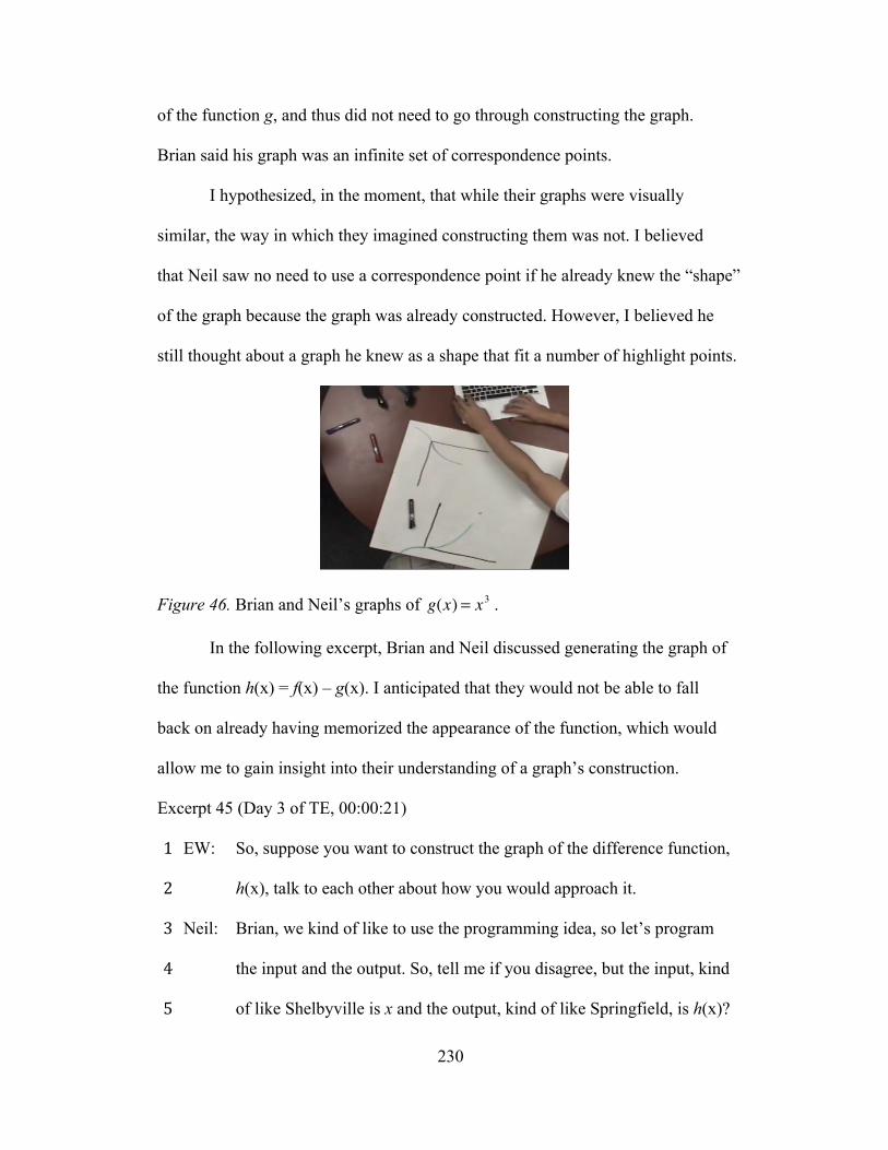
!
230
of the function g, and thus did not need to go through constructing the graph.
Brian said his graph was an infinite set of correspondence points.
I hypothesized, in the moment, that while their graphs were visually
similar, the way in which they imagined constructing them was not. I believed
that Neil saw no need to use a correspondence point if he already knew the “shape”
of the graph because the graph was already constructed. However, I believed he
still thought about a graph he knew as a shape that fit a number of highlight points.
Figure 46. Brian and Neil’s graphs of .
In the following excerpt, Brian and Neil discussed generating the graph of
the function h(x) = f(x) – g(x). I anticipated that they would not be able to fall
back on already having memorized the appearance of the function, which would
allow me to gain insight into their understanding of a graph’s construction.
Excerpt 45 (Day 3 of TE, 00:00:21)
EW: So, suppose you want to construct the graph of the difference function, "!
h(x), talk to each other about how you would approach it. #!
Neil: Brian, we kind of like to use the programming idea, so let’s program $!
the input and the output. So, tell me if you disagree, but the input, kind %!
of like Shelbyville is x and the output, kind of like Springfield, is h(x)? &!
g(x) = x3
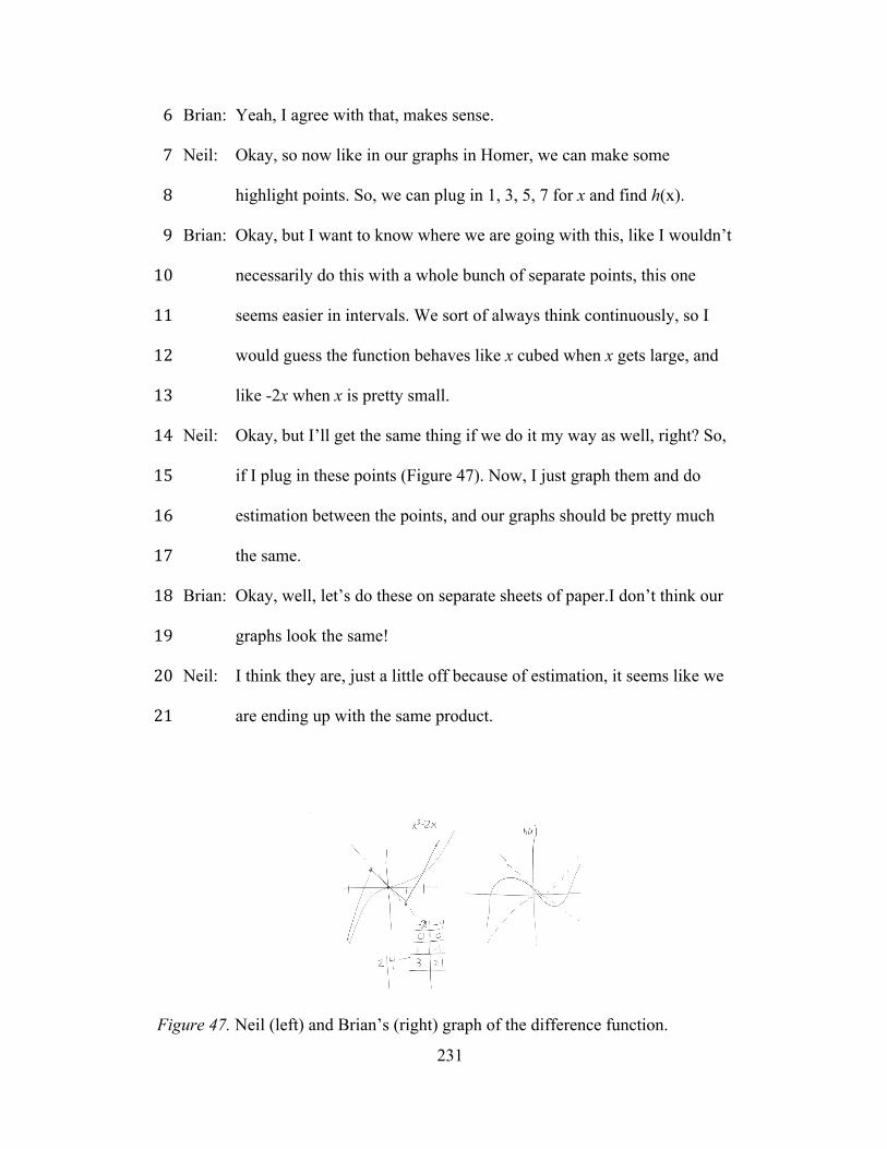
!
231
Brian: Yeah, I agree with that, makes sense. '!
Neil: Okay, so now like in our graphs in Homer, we can make some (!
highlight points. So, we can plug in 1, 3, 5, 7 for x and find h(x). )!
Brian: Okay, but I want to know where we are going with this, like I wouldn’t *!
necessarily do this with a whole bunch of separate points, this one "+!
seems easier in intervals. We sort of always think continuously, so I ""!
would guess the function behaves like x cubed when x gets large, and "#!
like -2x when x is pretty small. "$!
Neil: Okay, but I’ll get the same thing if we do it my way as well, right? So, "%!
if I plug in these points (Figure 47). Now, I just graph them and do "&!
estimation between the points, and our graphs should be pretty much "'!
the same. "(!
Brian: Okay, well, let’s do these on separate sheets of paper.I don’t think our ")!
graphs look the same! "*!
Neil: I think they are, just a little off because of estimation, it seems like we #+!
are ending up with the same product.#"!
Figure 47. Neil (left) and Brian’s (right) graph of the difference function.

!
232
Neil thought he and Brian agreed on how to program the correspondence
point (Excerpt 45, lines 3-5). However, Neil’s work suggested to me that he was
finding highlight points and estimating the graph between those points (Excerpt
45, lines 7-8), while Brian thought about the graph as an infinite number of
correspondence points, the behavior of which would depend on the value of x, f(x)
and g(x) (Excerpt 45, lines 9-13). Neil believed that the graphs (products) were
about the same (Excerpt 45, lines 20-21), and attributed differences in the graphs
to estimation. His description of similarity appeared to be based on the graphs
possessing similar shapes.
I believed Neil was thinking about a graph as a shape that fit a number of
points resulting from choppy covariation. By this, I mean that he imagined the
highlight points representing two values simultaneously, but estimation
(interpolation) was necessary because there were only a finite number of highlight
points. I was not yet convinced that Neil thought about a familiar function’s graph
without imagining highlight points.
I anticipated that asking Neil and Brian to construct the graph of a
function on the whiteboard without lifting their marker would help me gain
insight into their understanding of a graph as a representation of two quantities
having covaried, or lack thereof. In addition, I hypothesized this activity would
allow me to gain insight into what Neil did understand about a graph because he
would be constrained from plotting points and doing estimation.

!
233
Excerpt 46 (Day 3 of TE, 00:00:42)
EW: So, I asked you to construct the graph of the function without lifting "!
the pen from the paper. Neil, what did you come to? #!
Neil: I couldn’t really generate a perfect function, I kind of had to calculate $!
in my head the points I knew I needed to go through, sort of like %!
looking ahead, but it was hard because I couldn’t mark them down so I &!
had to think about where they would be and follow the trend through '!
the highlight points to make the graph. (!
Brian: It’s weird, I can kind of see what you are saying, but I don’t do it the )!
same way. I kind of just considered the graphs of the two functions, so *!
I could think about m(x) like a difference function as before, then "+!
focused on which intervals of x would correspond to where 2x2 or -4x ""!
would weight more (Figure 48). "#!
EW: Neil, what do you think about what Brian said? "$!
Neil: Well, again, we sort of are doing the same thing, making the graph, "%!
just going about it differently. I make some points and follow the trend "&!
of those points, and Brian just seems to decide on the trend before "'!
making any points, kind of like skipping a step. "(!
Figure 48. Neil (left) and Brian’s (right) graph created without lifting the marker.

!
234
Neil appeared to be creating both correspondence and non-correspondence
points while keeping his marker on the whiteboard (Excerpt 46, lines 3-7). His
graph relied on both plotted points and another set of points that created a path
between those plotted points. However, the two types of points did not represent
the same quantities. I anticipated it would be critical for Neil to think about a
graph as created by a point that always represented a correspondence because he
did not have an image of two quantities’ having values over a continuum, which
allowed him to think about “filling in” between the highlight points.
Brian generated the difference function graph by focusing on the behavior
of more familiar functions (Excerpt 46, lines 8-12). Brian’s description fit with his
process of programming a correspondence point and tracing it out continuously.
In this case, he was programming the correspondence point to represent a
difference of two familiar functions. I anticipated his image of continuous
covariation would allow him to interpret a given graph of a function by imagining
it as generated by a correspondence point having been traced out.
My analysis of Day 3 suggested that Neil was thinking about a graph as a
shape, situated in the plane, that fit a number of highlight points. In contrast, I
believed Brian was thinking about a graph as created by a correspondence point
traced out continuously in the domain of a function. I described Neil’s thinking as
similar to novice shape thinking and Brian’s thinking as similar to expert shape
thinking. However, I believed that Neil was at a point where his thinking could
become more advanced. I thought Neil was at a point where thinking about a
correspondence point creating a function’s graph continuously would rely on his

!
235
having an image of the simultaneous variation of quantities. I hypothesized that if
he thought in this way, he potentially could develop and image of the
correspondence point continuously tracing out a graph.
Day 4 - Sweeping Out a One-Variable Function
I evaluated my hypotheses in the sweeping out activity by 1)
understanding in what ways Brian and Neil thought about a graph as the result of
a continuous tracing out and 2) documenting how they responded to thinking
about a sweeping out of a function in the plane and its relationship to a surface in
space. I anticipated that an image of continuous tracing out fit with Brian’s
understanding, and that I could build on his notion of a correspondence point to
think about a graph being swept out in three dimensions. I anticipated that Neil’s
way of thinking about highlight points would constrain him from thinking about a
continuous sweeping out of a graph in the plane.
Brian and Neil agreed that defining a new function m(x) = ah(x) would
affect only the output values of the function. Brian described the effect of a as a
“vertical stretch” of the graph as the outputs changed and Neil anticipated that a
would be the factor by which the y-value of the “significant, highlight points
would move upward”. In both cases, they visualized a transformation in the
dependent quantity, but Neil appeared to believe the transformation only affected
the highlight points.
Excerpt 47 (Day 4 of TE, 00:00:15)
Brian: So, here’s how I think about a. It only affects the h(x), so the "!
function’s output becomes a times as large. It’s also kind of like #!
!
236
making the difference between the two functions which created h(x) a $!
times as large. I think the graph would reflect that, where you shift, %!
well, program the correspondence point to be five times as large &!
vertically, then trace out. '!
Neil: Yeah, I see what you are saying, where the a value affects the output (!
value for the function, it definitely doesn’t change the x. You sort of )!
anticipated it ahead of time, kind of made a plan, where I just think *!
about creating points for h(x) then the y-value gets multiplied by a, so "+!
you move those points up, and the slope of the graph between the ""!
points you chose gets more pronounced. "#!
Brian: What do you mean by the slope gets more pronounced? "$!
Neil: Um, slope of the lines connecting the major points could get steeper or "%!
less steep, they probably wouldn’t keep the same level of steepness. "&!
Brian: Okay, well I wasn’t really talking about steepness, I was imagining all "'!
the points moving up, not a few points which you seem to be "(!
indicating with your hands. ")!
Neil: Well, moving a few points takes the rest of the graph with it because "*!
the graph has to fit the trend of the points. #+!
Brian’s description of the effect of a on every correspondence point
allowed him to visualize the entire graph stretching vertically by a factor of a
(Excerpt 47, lines 1-3). He anticipated that a would affect the dependent quantity,
which allowed him to imagine programming a correspondence point with x and
ah(x) as values (Excerpt 47, lines 4-6). Neil appeared to visualize the vertical

!
237
stretch occurring only for the highlight points, but eventually all points moved
because the transformation of the highlight points dragged the other points with it.
(Excerpt 47, lines 8-9). I believed he thought about the graph bending to
accommodate the isolated points that stretched vertically (Excerpt 47, lines 10-12).
Neil was imagining the graph between the highlight points as a shape with
physical properties which needed to fit the trend (Excerpt 47, lines 19-20).
After this exchange, Brian asked Neil what would happen if he could use
more highlight points. Neil said the graph would just be laid over them [highlight
points] and become “better fitting”. His description of better fitting indicated he
imagined the graph becoming a better approximation, but it was not clear to what
the graph became “better fitting”. I believed he thought that more highlight points
(e.g. adding 5) was a better approximation to a graph composed of an infinite
number of highlight points.
Neil assumed that he and Brian were constructing graphs in the same way
because the graphs appeared to share the same features. Brian clearly saw a
difference in his and Neil’s thinking, which he characterized as thinking about
how graphs were made in separate ways. While they both used the notion of a
correspondence point to generate their graphs, Neil imagined that a
correspondence point existing only where it was calculationally convenient, while
Brian attended to the correspondence point sweeping out continuously to generate
a function’s graph. It seems this difference could have been attributed to their
goals. Neil believed a finite number of correspondence points in tandem with
estimation were sufficient to create the same graphs that Brian generated.
!
238
Midway through Day 4, I asked Brian and Neil to think about the value of
a as representing the distance in front of (for positive values of a) or in back of
(for negative values of a) of the current function’s graph. Neil commented that a
= -3 created the function’s graph, and also situated it 3 units behind the computer
screen. Brian noted that as a increased from positive to negative numbers, the
function’s graph would travel through the computer screen.
Excerpt 48 (Day 4 of TE, 00:00:39)
EW: Right, so let’s pick up, we just talked about how to think about a, what "!
did you guys hear me say? #!
Neil: I’ll take a shot, okay Brian? Yeah, well basically we are thinking about $!
a corresponding to another axis, but this one comes out of the laptop %!
screen, so it kind of represents depth where the zero depth is the laptop &!
screen. '!
Brian: I agree with that, it turns into thinking mostly in space. (!
EW: Can you say more about thinking in space, each of you? )!
Brian: Mind if I take this first? [Neil nods] Now, what you do is kind of think *!
about stringing together a point that generates the graph in the plane "+!
from a sweeping out, and then we move that plane, corresponding to a ""!
value of a, and that traces out a surface. It’s not totally right, but we "#!
kind of have a correspondence graph consisting of correspondence "$!
points (Figure 49). "%!
EW: Neil, what did you hear Brian say, what do you think? "&!

!
239
Neil: I’m a little confused about all the sweeping out, but I can see how he "'!
might be relating it to the Homer situation again. Again, I kind of "(!
focus on making highlight points, except these are highlight graphs. So ")!
I would generate the graph for values of a, umm, like -2, 1, 3, 5, then "*!
fit the general trend between those graphs in space. #+!
EW: So what is going on between those values of a? #"!
Neil: I’m not sure because I picked those values of a, I’d have to pick all ##!
those values of a, which isn’t possible. So I pick the highlights and #$!
estimate between them, sort of like I did without the third axis. #%!
EW: Brian? #&!
Brian: I think it is possible to account for all values of a, just by sweeping out #'!
it covers all of the values.#(!
Figure 49. Neil and Brian’s depictions of viewing h(x) sweeping out.
Neil and Brian’s words and gestures indicated that they were thinking
about an object being created in three dimensions (Excerpt 48, lines 1-7). Brian

!
240
referred to this generating graph as a correspondence graph, likely trying to draw
a parallel between sweeping out in space and sweeping out a one-variable
function in the plane (Excerpt 48, lines 12-13). Neil indicated a highlight graph
was the result of fitting together graphs in the plane, corresponding to integer
values of a (Excerpt 48, lines 19-20). He believed that he could pick graphs
between those highlights graphs, but that would require picking “all” the values of
a, which he saw as cumbersome. (Excerpt 48, lines 22-24). I believed, in the
moment, that Neil thought that he would have to make a new graph for every
possible value of a, which would have required an infinite number of graphs.
Brian visualized that the process of sweeping out a one-variable function in a
plane would account for all values of a (Excerpt 48, lines 26-27).
Figure 50. Neil’s illustration of cross sections in space at integer values of a.
Neil appeared to imagine a process of “taking a snapshot” at every integer
value of a and he connected those graphs by interpolation, or trend fitting. I
characterized his thinking as imagining approximate planar regions, which fit
with his process of estimation for a graph of a one-variable function. Neil seemed
to imagine that the relationship between quantities’ values only existed at the tick
marks, often corresponding to integer values, but at the same time, he could
!
241
imagine that he needed to make an infinite number of graphs at values of a to
create a surface.
To communicate what he was seeing “in his mind”, Neil defined a two-
variable function and attempted to graph it on the whiteboard (Figure 50). Brian
joined in, and together, they constructed a set of axes, consisting of x, a, and z,
and noted that a was similar to y. The convention of z was their own, but they said
it was natural to pick z already having x and y. They were able to generate an
accurate sketch of the function, but Brian believed they were not constructing the
graph the same way because Neil was only estimating. Neil continued to believe
if they generated the same graph, then their method of constructing the graph
must be closely related.
I began Day 4 with the goal of gaining insight into how Neil and Brian
thought about the continuous tracing out of a function by a correspondence point
and correspondence graph in the plane. Each time Brian referred to a, he
described it as a continuous interval from which he could pick a plane to describe
the function’s behavior. Neil used a as a parameter without imagining it as a
variable which simultaneously represented all possible values of a as Brian had. It
seems that Neil did not see a need for thinking about what he was doing as a
special case of generating all possible functions over an interval of values for a. In
contrast, I believed that Brian visualized the function sweeping out continuously
along the a axis.
!
242
Day 5 - Generating Functions from Perspectives Day 5 focused on Neil and Brian generating functions from various
perspectives, which they had initially introduced when constructing the z and a
axes in Day 4. In the following excerpt, Neil and Brian exchanged thoughts about
the role of a in generating a two-variable function.
Excerpt 49 (Day 5 of TE, 00:00:10)
EW: Brian, I noticed that you commented about a being like another "!
variable. Could you say more? #!
Brian: Yeah, basically I was thinking that because I am tracing out along $!
another axis, and for all the values, a is kind of like another variable, %!
where my height above the axes depends on both x and a. &!
Neil: I see what Brian is saying, our output, which seems to be the, what, z '!
axis? That depends on the value of x and a. I guess I would call them (!
both variables, containing the highlight points. )!
Brian: Well, I can’t get past this highlight point thing, I think of everything as *!
a highlight point, like, uh, you are describing them. "+!
EW: Okay, so, how would you define the function? ""!
Brian: Well, I think f(x,a) because they are both variables. [Neil nods]. "#!
EW: Okay, so take me through the process you would use to generate the "$!
graph of a function of two variables then. "%!
Brian: I think I’d do the programming thing overall, but I noticed in GC that "&!
it is normal to use z, x and y, so I’ll call y like a, and z is like the output "'!
of the function. So I can either look at z and x for fixing values of y, "(!

!
243
like a parameter, or z and y, for fixing values of x, where x is like a ")!
then. I’m guessing the graph you get is smooth, sort of like all the "*!
correspondence points but now we have to program each point with #+!
three pieces of information. #"!
Neil: Hold on, I’m not sure what you mean all the correspondence points. ##!
I’m imagining that we take some highlight functions from the z-x #$!
perspective and z-y, then sort of estimate the general trend between #%!
them to build up the graph. #&!
Brian: Why would we need to estimate, when we know the function so we #'!
can be exact? #(!
Neil: It would take infinitely long, you’d have to make all the points #)!
individually, and estimation is better. You can sort of lay the surface #*!
accurately then.$+!
I interpreted Brian’s description of a parameter value to mean he imagined
an infinite number of highlight points, which he called correspondence points
(Excerpt 49, lines 9-10, 19). I believed that he imagined that highlight points
resulted from programming the correspondence points with three pieces of
information (Excerpt 49, line 21), which he indicated were x, a, and f(x,y). I
continued to hypothesize that Brian thought a function’s graph could not exist
without correspondence points, and the correspondence points could not exist
without relationships between dependent and independent quantities (specified or
unspecified). This created the necessity for him thinking about a function’s graph

!
244
as a representation of a relationship between quantities which he visualized by
using perspectives.
Neil agreed with Brian’s use of the z-x and z-y perspectives (Excerpt 49,
lines 24-25), but believed it was necessary, and sufficient, to use estimation
(Excerpt 49, lines 24-25) because making all the points individually would take
forever (Excerpt 49, lines 28-30). Neil’s responses suggested to me that he was
thinking about plugging in and graphing every correspondence point individually,
and he used highlight points and estimation to cope with the impossible task of
graphing an infinite number of points. However, even if he had thought about a
graph as an infinite number of correspondence points, he still imagined creating
the graph as like laying the surface (Excerpt 49, lines 29-30). I believed, in the
moment, that Neil thought a function’s graph, in the plane or in space, was a
covering laid over a number of highlight points or highlight graphs.
Just after the discussion in Excerpt 49 (Day 5), Neil noted that he was
trying to deal with an information overload from trying to graph a million points.
He said that in both functions of one and two variables, the graphs must be
estimated by the general trends of highlight points to construct the graph. Brian
responded that there were an infinite amount of points on a graph, but he did not
need to generate them all. Instead, he described the programming of a
correspondence point to “operate” on each point. It appeared that Neil thought
about the correspondence point as a program he would need to run for every (x,y)
pair, while Brian was thinking about the correspondence point as a repeatable
!
245
process with general instructions for representing the output resulting from each
(x,y) pair.
I believed that Neil’s solution was to limit the number of times he had to
type information into a program by choosing the types of points he would
program. Neil did not use his programming metaphor to describe the “estimation”
portion of his graphs. As a result, he was not thinking about those areas of the
graphs as having been programmed. In constrast I believed that Brian imagined
every point as the result of a programmed correspondence point.
Day 5 - Interpreting the Graph of a Two-Variable Function
After a short break in Day 5, I provided Brian and Neil with the graph of a
two-variable function and asked them to describe a possible function that the
graph could represent. I anticipated that Brian would focus on how each
perspective of the graph was programmed to generate the surface, while Neil
would see the surface as a covering laid over highlight points.
Excerpt 50 (Day 5 of TE, 00:01:01)
EW: Okay, so what we have here is a graph of a function in space (Figure 51, "!
right). I’d like you to discuss how you think it was created, as in what #!
function could have generated it, based on your understanding. $!
Neil: Okay, since we were talking about perspectives, so I think of this graph %!
as kind of a surface laid over a bunch of exact points, and it fills in &!
between to get some estimation. '!
Brian: But that can’t help us figure out what function’s graph we have. (!
!
246
Neil: Sure it can, you’d just need to figure out a commonality between those )!
points, and kind of view the general trend of the overlaid graph. So, for *!
example, if the y is twice as much as the x in the points, we could have "+!
part of our function be y = 2x. ""!
Brian: I don’t understand, you’d basically be guessing then, right? "#!
Neil: No, but it would be hard, I don’t see another way really at all I guess. "$!
Brian: What about perspectives, like we’ve been talking about? I think we "%!
could pick a z-x and z-y perspective, and also an x-y, where the "&!
variable not included becomes the parameter and look at the graph to "'!
see what function might have made that perspective? "(!
Neil: Won’t that just make us estimate a point from a general trend anyway? ")!
Brian: No, it seems like you want to look at the trend of the whole surface, "*!
which I think is pretty much impossible, we have to consider the z-x, z-#+!
y and x-y, and see if we can get them to agree on some kind of function. #"!
EW: Neil, can you say more about how you think your and Brian’s ##!
approaches agree, and how they compare to what we’ve talked about so #$!
far? #%!
Neil: Okay, no offense, but I think you guys are talking about a fancier way #&!
of doing things than we need to. It’s just a bunch of points and #'!
estimation is good enough, guessing the general trend. I think my #(!
highlight points or functions approach ends up with the same thing.#)!
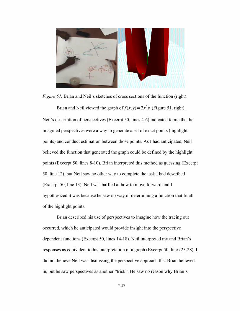
!
247
Figure 51. Brian and Neil’s sketches of cross sections of the function (right).
Brian and Neil viewed the graph of f (x, y) = 2x2y (Figure 51, right).
Neil’s description of perspectives (Excerpt 50, lines 4-6) indicated to me that he
imagined perspectives were a way to generate a set of exact points (highlight
points) and conduct estimation between those points. As I had anticipated, Neil
believed the function that generated the graph could be defined by the highlight
points (Excerpt 50, lines 8-10). Brian interpreted this method as guessing (Excerpt
50, line 12), but Neil saw no other way to complete the task I had described
(Excerpt 50, line 13). Neil was baffled at how to move forward and I
hypothesized it was because he saw no way of determining a function that fit all
of the highlight points.
Brian described his use of perspectives to imagine how the tracing out
occurred, which he anticipated would provide insight into the perspective
dependent functions (Excerpt 50, lines 14-18). Neil interpreted my and Brian’s
responses as equivalent to his interpretation of a graph (Excerpt 50, lines 25-28). I
did not believe Neil was dismissing the perspective approach that Brian believed
in, but he saw perspectives as another “trick”. He saw no reason why Brian’s

!
248
approach would end with a more “correct” result (a graph) than his own. Neil
likely believed it was sufficient to produce a “good enough” graph, using his
process of estimation. It is plausible he saw Brian’s process as unnecessarily
complicated.
When Brian saw a graph in space, it appeared that he saw an infinite
number of correspondence points. These points could be generated from the z-x,
z-y or x-y perspectives. Thus, he focused on reverse engineering his method of
constructing function’s graphs via a “program”. He did this to deduce the program
that generated the given graph. Neil also attempted to reverse engineer from his
construction of a graph, but I believed because his process for constructing a
graph relied on picking highlight points and doing inexact estimation, he saw no
way to reverse the process given an already constructed graph in space.
Part I Conclusions
Brian’s ways of thinking about functions.
During Day 1, I noted that Brian was focused on tracking quantities’
values as they varied. He understood that as long as Homer, Springfield and
Shelbyville existed, Homer’s distance from Shelbyville and Springfield existed.
Then, as Homer moved on the road, the distances varied simultaneously. While I
cannot attribute Brian’s thinking about a graph solely to one activity in this
teaching experiment, it appeared the Homer activity allowed Brian to think about
a function’s graph as created by the sweeping out of a correspondence point,
which simultaneously represented two values. This way of thinking not only

!
249
allowed him to imagine how a graph was constructed, but helped him thinking
about every graph as generated by an infinite number of correspondence points.
My model for his thinking indicated that he began thinking about
“programming the correspondence point” to move in a particular way by tracking
the independent and dependent variables. He imagined sweeping out a one
variable function in a plane from multiple perspectives, each generating the same
surface in space. He interpreted the surface of a function’s graph as an infinite
number of correspondence points, each programmed with three pieces of
information. Brian’s understanding of how a surface in space was constructed
then helped him hypothesize about what function could represent a “mystery”
surface in space.
Neil’s ways of thinking about functions.
The Homer activity suggested to me that Neil was thinking about using
highlight points as a way to estimate the correct shape of a function’s graph. I
described his way of thinking as choppy covariation, in which Neil was imagining
highlight points existing, programmed by the value of the independent and
dependent variable, but only at discrete points. By discrete, I mean that he only
tracked the quantities’ values as certain instances (e.g. specific locations of
Homer on the road) to produce “exact measurements”, and estimated the behavior
of the graph elsewhere. I believed that Neil did not imagine the quantities’ values
varying simultaneously over those “breaks”. He believed the best way to
approximate the graph was to use linear interpolation. However, it remained
unclear what he was attempting to approximate.

!
250
I thought Neil was thinking about a graph as a wire or a mat overlaid on a
set of highlight points. While he appeared to program the highlight points in the
same way that Brian did, he did not imagine tracking the independent and
dependent values over a continuous interval of each quantity. Neil was so intent
on the end product (the graph) appearing to be the same as Brian’s that any
difference in how the function’s graph was constructed was unimportant to him.
Part II: Brian and Neil’s Ways of Thinking about Rate of Change
Table 21 !Brian and Neil’s Rate of Change Task Sequence.
Task Description Date (Day) Car A – Car B: Interpreting Meaning of the Graph 5/13/2011 (6) Car A – Car B: Measuring Rate of Change Using
the Graph 5/13/2011 (6)
Generalized Rate of Change Function and Direction
5/15/2011 (7) 5/17/2011 (8)
I anticipated that Neil and Brian would rely on the notion of a calculus
triangle to measure rate of change because of their use of it in class and during
tutoring sessions. I also believed that Neil and Brian’s interpretation of the
meaning of rate of change relied on thinking about average rate of change as a
constant rate of change of “another car going the same distance in the same
amount of time as the original car, but with its cruise control on”. This was the
primary analogy they used during our pre-teaching experiment sessions.
Days 6 and 7 - Car A-Car B and Rate of Change
I anticipated that because Neil and Brian relied on programming a
correspondence point or correspondence graph as a way to describe graphs of one

!
251
and two variable functions, they would continue to use programming as a way to
think about the behavior of a rate of change function.
Neil and Brian interpreted the crossing of graphs of Car A and Car B as an
indication that they were traveling the same speed after one minute of time had
elapsed. Brian and Neil both noted that the cars had identical average
accelerations because the change in speed and change in time were equivalent for
both cars. Neil said that “this is our usual way of thinking about average rate of
change, if the changes in the top are the same as the changes in the bottom, then
that means the average rates of change are the same.” Brian agreed with Neil, but
that the rates of change were not the same between those two points in the domain.
Excerpt 51 (Day 6 of TE, 00:00:13)
EW: Alright, so you two seem to be focused on the rate of change of the "!
function graphed here. Can you say more about the rate of change? #!
Brian: Yeah, well, I guess I was gonna say that you program an input, like $!
where you want to know the rate of change, then use the open form %!
rate of change as the output. But we have talked about using a &!
correspondence point, so I want to go at it that way, so the two things '!
the point needs is an x and rf (x) (!
EW: Okay, and what is rf (x) ? )!
Brian: It is the open form rate of change, so for some fixed value of h. So in *!
class, I would say if h is .05 then the value for the open form is like a "+!
constant rate of change, same distance, same time sort of thing. ""!
EW: Neil? Did you want to add anything? "#!
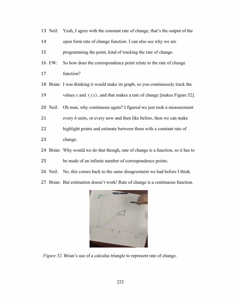
!
252
Neil: Yeah, I agree with the constant rate of change, that’s the output of the "$!
open form rate of change function. I can also see why we are "%!
programming the point, kind of tracking the rate of change. "&!
EW: So how does the correspondence point relate to the rate of change "'!
function? "(!
Brian: I was thinking it would make its graph, so you continuously track the ")!
values x and rf (x) , and that makes a rate of change [makes Figure 52]. "*!
Neil: Oh man, why continuous again? I figured we just took a measurement #+!
every h units, or every now and then like before, then we can make #"!
highlight points and estimate between them with a constant rate of ##!
change. #$!
Brian: Why would we do that though, rate of change is a function, so it has to #%!
be made of an infinite number of correspondence points. #&!
Neil: No, this comes back to the same disagreement we had before I think. #'!
Brian: But estimation doesn’t work! Rate of change is a continuous function. #(!
Figure 52. Brian’s use of a calculus triangle to represent rate of change.

!
253
Brian used a calculus triangle to represent the quantities he was measuring
in the open form rate of change (Figure 52). At the same time, he considered how
to program a correspondence point to represent the rate of change function. His
description of the rate of change as continuous (Excerpt 51, lines 3-5), indicated
that he imagined “programming” the rate of change function as he would in the
Homer activity. He programmed the correspondence point with x and the open
form rate of change function rf (x) (Figure 53), and imagined these values
simultaneously varying (Excerpt 51, lines 18-19). I believed, in the moment, that
Neil was thinking about highlight points of the function being available only
when the independent variable increased in increments of h (Excerpt 51, lines 20-
21). Neil’s comment that he would estimate between the highlight points using a
constant rate of change (Excerpt 51, lines 22-23) may have been his connection
between linear estimation and constant rate of change as a linear function.
Figure 53. Open form rate of change and Brian’s original calculus triangle.
Brian believed that h had no effect on the selection of highlight points
every h units because to him, h specified the interval over which the rate of
change was being measured. Neil insisted that every rate of change function
comes from estimation, and he indicated that if we were able to zoom in on the
graphs in the Car A- Car B situation, there would be linear segments connecting
highlight points.
!
254
Neil’s use of highlight points fit with his thinking about the shape of the
graph as more important than the correspondence points. Because he knew that a
linear function’s graph was associated with constant rate of change, he was able to
justify his estimation technique between highlight points. I anticipated that for
Neil to make any shift from thinking “every h units”, he would need to encounter
the graph of a rate of change function that did not fit with his anticipation of linear,
connected segments.
Day 7 – Programming a Rate of Change Function
At the beginning of Day 7, I used Graphing Calculator to allow Brian and
Neil to explore their conjectures about how to construct a rate of change
function’s graph. Brian and Neil worked on programming the rate of change
correspondence point, and debated about the smoothness of the resulting graph.
Excerpt 52 (Day 7 of TE, 00:00:12)
EW: Right, so let’s get to this one. You two seem to be at a crossroads "!
about how to generate the function, so I thought we would do it in GC. #!
Neil: Can I pick a function? How about a cubic function, those are good. $!
EW: Alright, so I want to program everything like you told me to before, %!
where this point will represent x and rf (x) (Figure 54), and you gave &!
me the definition of open form before. Now, if we traced the '!
correspondence point out, it would produce a graph, each of you tell (!
me about the graph. )!
Neil: I’ll start, I basically think it is going to be a bunch of linearly *!
connected segments between hinge, er, highlight points, linear slope "+!

!
255
between. Because GC takes certain measurements because it can’t take ""!
every possible one, and does a best guess between. "#!
Brian: No surprise, I guess, I disagree, I think the graph is going to be smooth, "$!
because GC does a correspondence like thing, and keeps track of them "%!
over super small intervals to make a smooth looking graph. "&!
EW: Alright, so if I increase the value of x, the correspondence point moves "'!
here [points to computer screen]. Now, if I graph the function, here it "(!
is, what do you notice? ")!
Neil: I guess it looks pretty smooth, but I don’t think it should. This is weird, "*!
I don’t see the highlight points I was expecting, but maybe there are a #+!
bunch of them. #"!
Brian: Hey Neil, try this, I think we actually are along the same lines, just ##!
imagine you have a huge number of highlight points. #$!
Neil: But that couldn’t work because at some point you have to estimate #%!
between them, it’s too many to do, but maybe GC did it your way here. #&!
Figure 54. The basis of discussion about programming a rate function.
Brian focused on generating a graph of the rate of change function while
understanding the x and rf (x) were simultaneously varying. This insight helped
!
256
Brian anticipate that the rate of change function’s graph would be smooth
(Excerpt 52, lines 13-15). Neil’s attention to the highlight points made the
smoothness of the rate of change function puzzling for him because he had
anticipated a function’s graph to be a number of linearly connected segments
(Excerpt 52, lines 9-12). Neil’s anticipation that there could be a large number of
highlight points (Excerpt 52, lines 20-21), but could not imagine actually
generating them (Excerpt 52, lines 24-25).
I turned the conversation to the continuous tracing out of a correspondence
point so there were highlight points everywhere. I created a Graphing Calculator
document that initially displayed only “highlight points”, which Neil had
calculated (Figure 55, purple points). Neil believed the function would connect
those points using “linear lines” because the general trend was linear. Brian
programmed a correspondence point (Figure 55, blue dot), which he said would
trace over the highlight points and every point between. I ran the animation, and
Neil confirmed that Brian’s assertion was accurate. Neil said, “Man, I think I sort
of see what is going on here, GC is using a whole bunch of highlight points
without really showing them.” Neil insisted that there was still estimation going
on between the highlight points, but could not describe where the estimation was
being generated.

!
257
Figure 55. Representing the rate of change function as a tracing out.
After Day 7, I believed that Neil attributed the difference in his thinking
and what he saw in the animation to an estimation process used by Graphing
Calculator. Brian saw his way of thinking about programming a point using a rate
of change function as identical to that of Graphing Calculator. Moving forward, I
attempted to use the notions of estimation and programming to gain insight into
how they would interpret and measure rate of change in space.
Day 8 - Interpretation of Rate of Change in Space
Day 8 began with a discussion about the meaning of rate of change at a
point in space. The previous sessions had focused largely on “how to graph” the
rate of change function. The following excerpt centered on how Neil and Brian
would interpret the meaning of rate of change at a point in space.
Excerpt 53 (Day 8 of TE, 00:00:02)
EW: How would you think about rate of change at a point in space? "!
Brian: My first though is that it has multiple rates of change, kind of like #!
sitting on a hill, depending where you look, the steepness, slope at that $!
point can be different. %!

!
258
Neil: I agree with that, I thought about the kind of example too, or just &!
sitting on the surface we swept out, maybe we can use the z-x and z-y '!
rates of change? (!
Brian: Yeah! Umm, let’s see though, if we want to make a rate of change )!
function and then graph it in space, we need to figure out a way to *!
program it, and do a sweeping out. "+!
Neil: What about just plugging in x, y and the rate of change? Oh, I guess ""!
we don’t know the rate of change yet, so my point thing wouldn’t "#!
work. "$!
Brian: Alright, for z-x, it is kind of like, okay let’s back up, let’s say we are at "%!
a point (a,b,c) in space. Then for z-x, we fix y at b, then do the normal "&!
rate of change except it has to be two-variables. "'!
Neil: Yeah, that makes sense, so we need an h, maybe like f(x+h,b)-f(x,y), "(!
then divided by h, and then for z-y, we just say y+h and fix x at a? ")!
Brian: Yeah, let’s go with that. "*!
EW: Okay, so where do you want to go next then, what is your plan? #+!
Brian: We need the two rates of change to make an overall rate of change #"!
function, then we can graph it by doing the sweeping out I think. ##!
Neil: I’d rather just draw the two calculus triangles that I am imagining each #$!
in a perspective. #%!
Brian’s description of rate of change (Excerpt 53, lines 2-3), indicated he
was thinking about rate of change in a direction “at” a point on the surface of the
function’s graph. Brian’s suggestion of considering multiple rates of change from
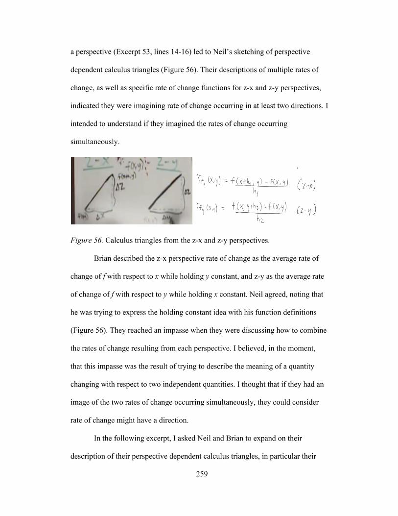
!
259
a perspective (Excerpt 53, lines 14-16) led to Neil’s sketching of perspective
dependent calculus triangles (Figure 56). Their descriptions of multiple rates of
change, as well as specific rate of change functions for z-x and z-y perspectives,
indicated they were imagining rate of change occurring in at least two directions. I
intended to understand if they imagined the rates of change occurring
simultaneously.
Figure 56. Calculus triangles from the z-x and z-y perspectives.
Brian described the z-x perspective rate of change as the average rate of
change of f with respect to x while holding y constant, and z-y as the average rate
of change of f with respect to y while holding x constant. Neil agreed, noting that
he was trying to express the holding constant idea with his function definitions
(Figure 56). They reached an impasse when they were discussing how to combine
the rates of change resulting from each perspective. I believed, in the moment,
that this impasse was the result of trying to describe the meaning of a quantity
changing with respect to two independent quantities. I thought that if they had an
image of the two rates of change occurring simultaneously, they could consider
rate of change might have a direction.
In the following excerpt, I asked Neil and Brian to expand on their
description of their perspective dependent calculus triangles, in particular their
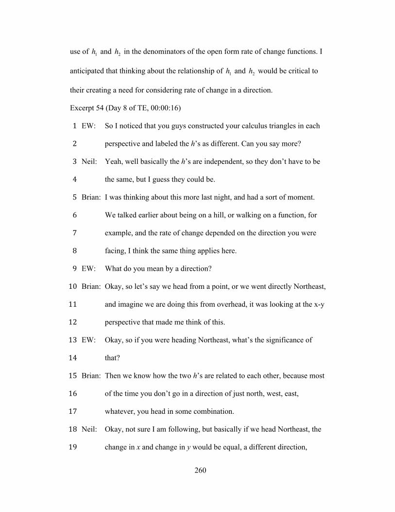
!
260
use of h1 and h2 in the denominators of the open form rate of change functions. I
anticipated that thinking about the relationship of h1 and h2 would be critical to
their creating a need for considering rate of change in a direction.
Excerpt 54 (Day 8 of TE, 00:00:16)
EW: So I noticed that you guys constructed your calculus triangles in each "!
perspective and labeled the h’s as different. Can you say more? #!
Neil: Yeah, well basically the h’s are independent, so they don’t have to be $!
the same, but I guess they could be. %!
Brian: I was thinking about this more last night, and had a sort of moment. &!
We talked earlier about being on a hill, or walking on a function, for '!
example, and the rate of change depended on the direction you were (!
facing, I think the same thing applies here. )!
EW: What do you mean by a direction? *!
Brian: Okay, so let’s say we head from a point, or we went directly Northeast, "+!
and imagine we are doing this from overhead, it was looking at the x-y ""!
perspective that made me think of this. "#!
EW: Okay, so if you were heading Northeast, what’s the significance of "$!
that? "%!
Brian: Then we know how the two h’s are related to each other, because most "&!
of the time you don’t go in a direction of just north, west, east, "'!
whatever, you head in some combination. "(!
Neil: Okay, not sure I am following, but basically if we head Northeast, the ")!
change in x and change in y would be equal, a different direction, "*!
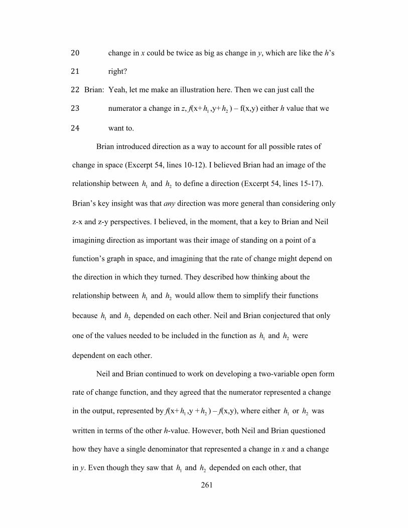
!
261
change in x could be twice as big as change in y, which are like the h’s #+!
right? #"!
Brian: Yeah, let me make an illustration here. Then we can just call the ##!
numerator a change in z, f(x+h1 ,y+h2 ) – f(x,y) either h value that we #$!
want to.#%!
Brian introduced direction as a way to account for all possible rates of
change in space (Excerpt 54, lines 10-12). I believed Brian had an image of the
relationship between h1 and h2 to define a direction (Excerpt 54, lines 15-17).
Brian’s key insight was that any direction was more general than considering only
z-x and z-y perspectives. I believed, in the moment, that a key to Brian and Neil
imagining direction as important was their image of standing on a point of a
function’s graph in space, and imagining that the rate of change might depend on
the direction in which they turned. They described how thinking about the
relationship between h1 and h2 would allow them to simplify their functions
because h1 and h2 depended on each other. Neil and Brian conjectured that only
one of the values needed to be included in the function as h1 and h2 were
dependent on each other.
Neil and Brian continued to work on developing a two-variable open form
rate of change function, and they agreed that the numerator represented a change
in the output, represented by f(x+h1 ,y +h2 ) – f(x,y), where either h1 or h2 was
written in terms of the other h-value. However, both Neil and Brian questioned
how they have a single denominator that represented a change in x and a change
in y. Even though they saw that h1 and h2 depended on each other, that

!
262
dependence did not immediately resolve their issue of what change to represent in
the denominator. I believed that this was because they were focused on trying to
represent a single change in the denominator while they understood that there
were changes in both x and y.
Excerpt 55 (Day 8 of TE, 00:00:49)
EW: So, what is your denominator in the function, your conjecture? "!
Brian: I was thinking either h-value, whichever you have in the numerator. #!
Neil: But doesn’t that kind of just delete it, it goes away? $!
Brian: No, you just define it in terms of h1 , if you are talking about h2 . %!
EW: So if one h is in the denominator, and we make that value small, what &!
happens to the other h value?? '!
Brian: Well, oh yeah, it becomes small as well, it’s not like the h’s have the (!
same value, but they can end up getting so small it doesn’t matter. )!
Neil: Ah, I see what you mean. So like in class we talk about making *!
changes so small, because we have an equation to relate the two h’s, "+!
then when one gets really small, the other one has to get smaller too? I ""!
was thinking multiply in the denominator I guess, but that doesn’t need "#!
to happen, you just need one of them to become small because they are "$!
related, the h’s I mean, so then both do. "%!
Brian: So, I guess that’s our overall rate function for two variables. Now we "&!
can sort of program the points to do the graph. "'!
Brian’s insight that the changes in x and y became smaller in tandem
allowed him to conjecture that using a single parameter in the denominator

!
263
(Excerpt 55, lines 7-8) was acceptable (Excerpt 55, line 2). Neil appeared to focus
on deleting one of the parameters, but Brian’s insight allowed him to think about
the equation they had specified between h1 and h2 . By imagining progressively
smaller values for h1 , he found that h2 became smaller as well given the
proportional relationship specified by choosing a direction in space (see Figure
57).
Figure 57. Brian and Neil’s open form two variable rate of change function.
Day 8 - Existence of Rate of Change at a Point in Space
Brian and Neil developed a two-variable rate of change function in
Excerpt 55 (Figure 57). Brian focused on how to think about generating the graph
of the rate of change function by a sweeping out. Brian did not think he could
assume rate of change existed at a point in space. He described how if one were
standing on a hill, the rate of change at that point would be different in most
directions. As a result, graphing a rate of change at a point would be impossible.
In the following excerpt, Brian and Neil expanded on this discussion.
Excerpt 56 (Day 8 of TE, 00:01:21)
EW: So now you have come up with a rate of change function for a two-"!
variable function, I know you wanted to talk about graphing the rate of #!
change function. $!
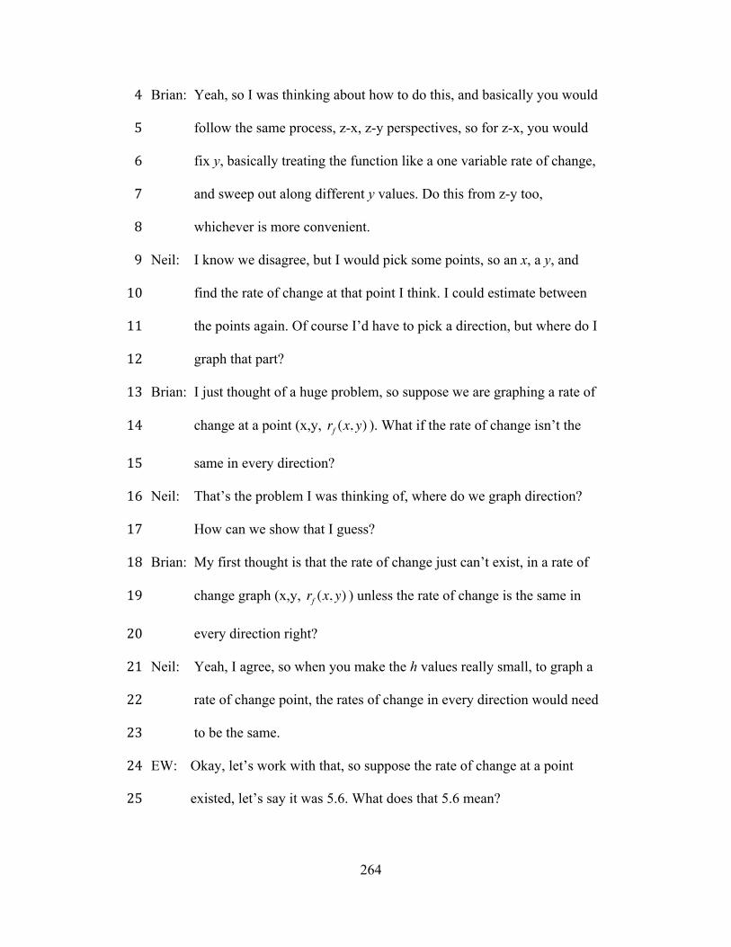
!
264
Brian: Yeah, so I was thinking about how to do this, and basically you would %!
follow the same process, z-x, z-y perspectives, so for z-x, you would &!
fix y, basically treating the function like a one variable rate of change, '!
and sweep out along different y values. Do this from z-y too, (!
whichever is more convenient. )!
Neil: I know we disagree, but I would pick some points, so an x, a y, and *!
find the rate of change at that point I think. I could estimate between "+!
the points again. Of course I’d have to pick a direction, but where do I ""!
graph that part? "#!
Brian: I just thought of a huge problem, so suppose we are graphing a rate of "$!
change at a point (x,y, rf (x, y) ). What if the rate of change isn’t the "%!
same in every direction? "&!
Neil: That’s the problem I was thinking of, where do we graph direction? "'!
How can we show that I guess? "(!
Brian: My first thought is that the rate of change just can’t exist, in a rate of ")!
change graph (x,y, rf (x, y) ) unless the rate of change is the same in "*!
every direction right? #+!
Neil: Yeah, I agree, so when you make the h values really small, to graph a #"!
rate of change point, the rates of change in every direction would need ##!
to be the same. #$!
EW: Okay, let’s work with that, so suppose the rate of change at a point #%!
existed, let’s say it was 5.6. What does that 5.6 mean? #&!

!
265
Neil: It still comes from an open form rate of change, like we had, so it is an #'!
estimate of average rate of change. #(!
Brian: Same here, but I don’t know how to phrase it. #)!
Neil: Something like the average rate of change of f with respect to x and y, #*!
that’s my best guess. $+!
Brian: Yep, and if we made h really small, we could probably find the closed $"!
form rate of change too. $#!
Brian and Neil’s insights about graphing a value for rate of change at a
point allowed them to conjecture that the rate of change could not be graphed
unless the rate of change at a point was the same in every direction (Excerpt 56,
lines 18-20). I believed they thought graphing a rate of change function required
an infinite number of perspectives, defined by a direction, of which z-x, z-y and
x-y were special cases. Brian and Neil’s consideration of the z-x, z-y and x-y
perspectives allowed them to think about those perspectives as special cases
(Figure 58). I believed that Brian and Neil’s insight that those three perspectives
were special cases of an infinite number of perspectives allowed them to
problematize rate of change at a point in space in ways that Jesse and Jori did not.
Figure 58. Brian’s illustration of rate of change at a point in space.

!
266
Part II Conclusions
Brian and Neil problematized how to interpret and calculate a rate of
change at a point in space because they were concerned with defining rate of
change at a point in space. Neil’s construction of “simultaneous calculus triangles”
and Brian’s reflection on them as a way to represent partial rates of change
indicated to me that they were imagining change occurring in different directions
in space. The x-y perspective allowed them to think about relating the
simultaneous changes in x and y by considering a direction, and supported their
construction of an open form rate of change function. By attempting to generate
the graph of the rate of change function, Brian, and then Neil, were able to
problematize the existence of rate of change at a point in space. They came to
understand that to “graph a point from the rate of change function”, the rates of
change would have to be invariant under direction. However, for this to be true,
the function would need to be constant.
Chapter Summary
In this chapter, I described the development of my inferences about the
thinking of two calculus students, Brian and Neil, who participated in a group
teaching experiment focused on functions of two-variables and their rates of
change. I hypothesized that Brian thought about a function’s graph as an infinite
number of correspondence points. I believed that Neil thought about a function’s
graph as a finite number highlight points with estimations between them. Lastly, I
showed how their use of programming a correspondence point supported their
interpretation and construction of a rate of change in a direction.

267
Chapter 8
CONCLUSIONS
In this chapter, I describe the results of my retrospective analyses. These
analyses considered the data from the three teaching experiments after the
teaching experiments had concluded. I intend to accomplish two things in this
chapter. First, I describe how my work contributes to, and builds on prior work of
the field with regard to what we know about student thinking about functions and
rate of change. Second, I characterize how my thinking has developed in regard to
the literature and method with which I framed my study. The goal of structuring
the chapter in this way is to provide the reader with an understanding of important
research questions to consider going forward, and how the development of my
thinking has prepared me to gain insight into those research questions.
Contributions
My analyses made at least three contributions to mathematics education.
First, my analyses built on Thompson’s description of shape thinking to describe
a tentative framework for a student’s association with a function’s graph. Second,
my analyses emphasized the importance of quantitative covariation for thinking
about rate of change, and showed how quantitative rate of change can be extended
from functions of one to functions of two variables. Third, my retrospective
analyses identified a number of surprising responses from students, each of which
has implications for future studies relative to student thinking about multivariable
functions and their rates of change. In the following sections, I explore each of
these contributions in greater detail.

268
Contribution 1: Types of Shape Thinking
Shape thinking is an association a student has with a function’s graph, and
shape thinking took on two forms in my study: novice shape thinking and expert
shape thinking. Novice shape thinkers might associate a shape with a particular
algebraic form (e.g., anything that looks like a “U” is a parabola and hence goes
with “ x2 ”, and vice versa). It is no more sophisticated than associating a name
with a face. The student does not think about the graph as a representation of
quantities having covaried. Expert shape thinking is thinking about a graph
emerging from the covariation of two or more variables. Novice shape thinkers
essentially ignore variation on axes and focus on the shape in the plane because
they do not see the graph as an emergent construction. Expert shape thinkers are
drawn naturally to think about variables on axes and how the variables’ values
interact because they associate the graph as an emergent representation of
covariation. In other words, the graph cannot exist independently of the
quantitative relationships it represents. In the remaining sections I describe expert
and novice shape thinking more completely and relate a hypothesized
developmental trajectory in relation to the teaching experiment sessions.
Expert shape thinking.
Expert shape thinking entails thinking about the graph of a function as the
result of simultaneously tracking the values of two or more quantities’ values.
This characterization of expert shape thinking relies on Thompson (2011) and
Saldanha & Thompson’s (1998) description of quantitative covariation in which

269
the student imagines that if two quantities covary, as one varies over an interval of
conceptual time, the other quantity varies over that same interval.
Jesse and Brian used tracing out and sweeping out as processes to imagine
constructing graphs of one and two-variable functions. Embedded in their image
of tracing out or sweeping out was an understanding that the resulting graph was a
representation of a relationship between two or more quantities. Implicit in that
way of thinking is that any feature of the graph, such as a shape, is a
representation of the behavior of two or more quantities. I believe Jesse and Brian
saw the surface in space as a representation because they could imagine sweeping
out a point in the plane to create a graph in the plane, which then swept out to
generate a surface in space, and each process depended on the variation of
quantities. For example, they imagined the sweeping out as a result of varying a
quantity, and then imagined tracking that sweeping out to create a representation
of the function. Implicit in this imagery is the notion that the definition of the
function provides the quantities’ values that are to be tracked. Expert shape
thinking also entails other ways of thinking: smooth continuous variation
(Castillo-Garsow, 2010; Saldanha & Thompson, 1998; Thompson, 2011),
covariation, and process conception of formulas.
In this study, students whom I characterized as expert shape thinkers
associated graphs with the correspondence point and graph in a plane that moved
perpendicularly to an axis. Thus, they associated the graph with the process used
to construct it. They imagined the resulting graph as composed entirely of
correspondence points. Expert shape thinkers might describe the graph as an

270
object in space, but they are also able to explain how that object is generated by
the relationship between the dependent and independent quantities’ values as they
vary. This image relies on the student imagining on simultaneous, continuous
covariation characterized by Thompson (2011) and Saldanha & Thompson (1998)
that allows the student to imagine how the graph was constructed.
Novice shape thinking.
Novice shape thinking entails associating a graph with an object in space,
but is not an emergent representation of quantities. For example, Jori thought
about classes of functions (e.g. cubic, linear) by associating them with a particular
shape. She did not always understand the graph as emerging from the function
definition, and even when she appeared to do so, she fell back on her focus on
shapes. Novice shape thinkers imagine the graph as an object situated in the
coordinate plane without reference to quantities’ values represented on the axes.
By imagining the graph as an object with properties independent of the
quantities in the function, the novice shape thinker focuses on properties like “the
graph goes up sharply”, without understanding how the definition of the function
and the scale of the axes create that feature of the graph. This also allows novice
shape thinkers to imagine changing the function definition and the graph of the
function independently of each other. For example, a vertical stretch of the graph
would not necessarily be accompanied by a change in the function definition, nor
would a change in the function definition necessarily require a change in the
graph. For example, Jori imagined that the graph in the Homer situation would
not be affected by exchanging the location of the two cities. I believe this was a

271
result of her not imagining how the quantities were to be represented on vertical
and horizontal axes. As a result, Jori was not attentive to how exchanging the
city’s locations would necessitate a reconstruction, if not a transformation, of the
prior graph.
When constructing the graph of a function, a novice shape thinker might
be unable to generate a graph unless the function fits an exemplar for which the
student has an image. This image might be the result of inputting a function into
graphing calculator numerous times. For example, Jori struggled to generate the
graph of the difference function because she was not sure how to incorporate the
shape of the two functions f (x) = x3,g(x) = 2x in the new graph. In general, I
believe that novice shape thinkers think about a graph by associating it with a
familiar shape, which might then be associated with a particular function.
However, this association turns the novice shape thinker’s attention from
visualizing how the graph could be an emergent representation. Thinking about
the graph in this way makes imagining the effect of a function transformation on
the graph, or the effect of a transformation of the graph on the function unrelated.
By this, I mean the student does not necessarily see a transformation in the graph
as a transformation of the function, and vice versa.
Transitions between novice and expert shape thinking.
My description of Jesse, Jori, Brian and Neil as novice or expert shape
thinkers was mostly categorical, and the focus of my study was not to move a
student from novice to expert shape thinker. As a result, I cannot define a

272
transition stage between novice and expert shape thinking, but I can use my data
to suggest the mechanisms by which I hypothesize this transition might occur.
My analyses characterized Jesse and Brian as mostly expert shape
thinkers, and Neil and Jori displaying actions consistent with both novice and
expert shape thinking. Jesse and Brian could use expert shape thinking to explain
that the shapes were a representation between quantities. Jori, and to a lesser
degree, Neil, relied on their association of graphs with familiar shapes, and then,
familiar function definitions. Both briefly explained a graph as a representation of
a function’s behavior, but when confronted with a graph, with which they were
not familiar, focused on shapes again. Based on these observations, I hypothesize
that a transition in shape thinking might occur in either direction. The transition
from expert shape thinker to novice shape thinker is implicit in being an expert
shape thinker. The student can focus on shapes, but when necessary, can think
about how those shapes are generated. I believe the transition from novice to
expert shape thinker requires the student to accommodate a new way of thinking
about a function’s graph being generated.
A preliminary framework for shape thinking.
My analyses suggest that shape thinking can be thought of in terms of a
developmental trajectory. This preliminary developmental trajectory can be
thought of as the beginning steps toward an explanatory framework composed of
constructs that I developed directly from my models of student thinking in the
teaching experiments. Within each column, I describe a way of thinking and
actions that could be evidence of a student thinking in that way.

273
Table 22.
A Tentative Framework for Shape Thinking.
Novice Shape Thinking Possible Transitions from Novice to Expert Expert Shape Thinking
Attention to the quadrants without regard to the coordinate axes on which quantities’ values are represented.
Attention to quadrants, but beginning to focus on the axes as related to the object in the quadrants.
A function’s graph as a representation of the quantities’ values represented by the Cartesian coordinates.
A function’s graph as an object, but not imbued with quantitative properties, and thus, not an emergent representation.
A function’s graph as a curve that fits a finite number of plotted points, but not an infinite number of points.
A function’s graph as a representation of a functional relationship using an infinite number of correspondence points.
A function’s graph as a wire that can be manipulated independently of the function definition.
A function’s graph can be manipulated, but because it becomes a different graph, a new function is required to fit that particular graph.
A function’s graph and its definition change simultaneously because they are representations of the same relationship between quantities.
A function definition as a set of symbols associated with a particular shape that the student calls the graph.
A function definition as a way to generate a finite number of points with which the student interpolates to create the function’s graph.
A function definition as a way to track two or more quantities’ values to generate a representation of the function.
Perspectives (z-x, z-y, x-y) are ways of looking at an already generated graph that the student thinks about as an object situated in the quadrants.
Generates a function’s graph from various perspectives, but does not understand that these perspectives generate equivalent surfaces in space.
Perspectives (z-x, z-y, x-y) as ways of imagining the two-variable function’s graph being generated while understanding each perspective will generate equivalent surfaces in space.
A two-variable function’s graph as a topographic map with a focus on its properties as if describing terrain.
A two-variable function’s graph as a map, where the features of that map are related to the specific function with which the student associates the graph.
A two-variable function’s graph as a map, where the features of the map are a result of representing the relationship between quantities.

274
It is important to note that the definitions of expert and novice shape
thinking are based on only the students in my study. I do not claim that expert
shape thinking explains how “experts”, such as mathematicians and scientists,
think about a graph of a function. Nor do I claim that most beginning students
think about a graph as a novice shape thinker. These constructs are an attempt to
explain and describe the students’ ways of thinking from this study, but do not
encompass all possible ways of thinking about a graph. Thus, the framework is an
initial step. It is plausible that there could be “expert-expert shape thinking”, in
which one thinks about a graph by focusing on its topological properties. If one
focuses on the topology of the surface, they focus entirely on the geometric
properties of that surface and the axes become irrelevant. However, because I did
not provide evidence that suggests a focus on topological properties as a plausible
hypothesis, it is not appropriate to include in this framework.
Contribution 2: Ways of Thinking about Rate of Change
My analyses, and my understanding of literature about quantitative
reasoning, covariational reasoning, and rate of change, suggest two ways to
characterize students’ ways of thinking about rate of change. 1) Non-quantitative
rate of change where the student focuses on rate of change as a number without
reference to a comparison between quantities as they are varying, and 2)
Quantitative rate of change as covariation describing how fast a quantity is
changing with respect to one (or two) quantities. In this section, I describe each of
these characterizations and explain how they rely on, and contribute to the notion
of quantitative covariation and rate of change I described in Chapter Two

275
(Castillo-Garsow, 2010; Saldanha & Thompson, 1998; Thompson, 2011; Carlson
et al., 2002).
Non-quantitative rate of change.
Students who think about rate of change without reference quantities
might, 1) Understand that to find a rate of change, they must identify changes in
two or more quantities and display some sophistication in how to algebraically or
graphically represent these changes, and 2) Interpret the resulting calculation or
ratio of changes without reference to the quantities change from which the
calculation resulted. This does not mean the students do not have an image for
variation. I believe they may have an image of each quantity having varied. They
might imagine that these quantities vary over conceptual time, so they imagine
observing a change in the quantities’ values over sub-intervals of conceptual time.
I believe their way of thinking breaks down because they may not have an image
of quantitative covariation, in which they imagine that two, or more, quantities
vary in tandem over that interval of conceptual time (Saldanha & Thompson
(1998); Thompson (2011)). Suppose that the student imagines the changes in two
or more quantities occurring independently of each other. A comparison of those
changes would then be a comparison of independent quantities, which might not
have a sensible interpretation. The student might wonder why it would be useful
to compare a change in z and a change in x if those two quantities varied
independently. However, if the student possessed an image of z and x covarying,
it is plausible that a comparison of the changes in z and x could describe how fast
the quantities were changing with respect to one another.

276
Jori used a tangent line, a single calculus triangle in the plane and slope to
represent her process for calculating a rate of change. I believe that she was
comfortable using these to “find” rate of change because she knew they accounted
for changes that were necessary to produce a rate of change. She knew she needed
to find changes to measure a rate of change, but she did not imagine those
changes to have occurred simultaneously. Thus, when I asked her to interpret a
result of the rate of change function, she rarely made references to how fast
quantities were changing in tandem because she did not originally imagine them
changing in tandem. At the same time, she sometimes displayed sophisticated
ways of thinking, particularly in the average speed activity. In the moment, she
thought about a comparison of distance and time, and interpreted the resulting
calculation as a rate. My analyses suggest that she drifted between focusing on the
calculation and trying to interpret the meaning of the calculation. However, when
trying to accommodate an interpretation of rate of change, she often relied only on
the accuracy of the calculation. Jori appeared to use calculational reasoning,
which led her to rely on the structure of the function, rather than the quantities
used to construct the rate of change function. Her calculational reasoning allowed
her to make significant progress in developing a rate of change function, but
simultaneously constrained her in interpreting the rate of change as a measure of
covariation.
Rate of change as a measure of covariation.
My characterizations of students’ thinking about rate of change as a
measure of covariation relies on Saldanha & Thompson (1998), Carlson et al.
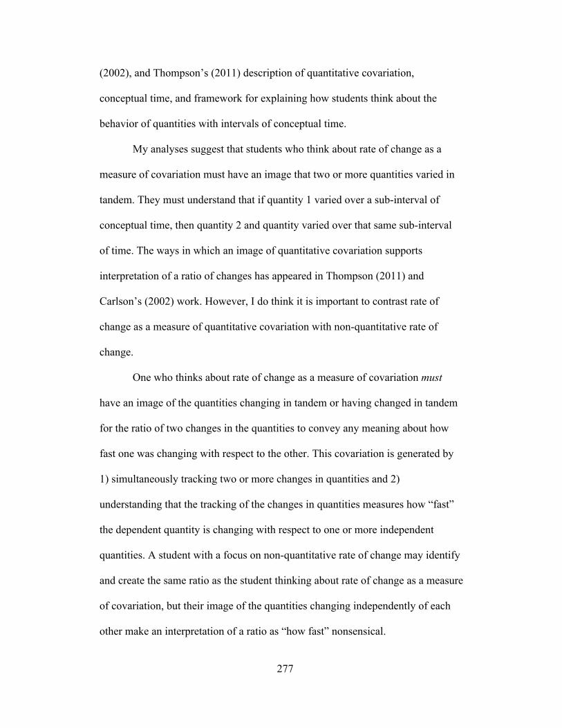
277
(2002), and Thompson’s (2011) description of quantitative covariation,
conceptual time, and framework for explaining how students think about the
behavior of quantities with intervals of conceptual time.
My analyses suggest that students who think about rate of change as a
measure of covariation must have an image that two or more quantities varied in
tandem. They must understand that if quantity 1 varied over a sub-interval of
conceptual time, then quantity 2 and quantity varied over that same sub-interval
of time. The ways in which an image of quantitative covariation supports
interpretation of a ratio of changes has appeared in Thompson (2011) and
Carlson’s (2002) work. However, I do think it is important to contrast rate of
change as a measure of quantitative covariation with non-quantitative rate of
change.
One who thinks about rate of change as a measure of covariation must
have an image of the quantities changing in tandem or having changed in tandem
for the ratio of two changes in the quantities to convey any meaning about how
fast one was changing with respect to the other. This covariation is generated by
1) simultaneously tracking two or more changes in quantities and 2)
understanding that the tracking of the changes in quantities measures how “fast”
the dependent quantity is changing with respect to one or more independent
quantities. A student with a focus on non-quantitative rate of change may identify
and create the same ratio as the student thinking about rate of change as a measure
of covariation, but their image of the quantities changing independently of each
other make an interpretation of a ratio as “how fast” nonsensical.

278
Both Jesse and Brian described how they would program the
correspondence point to trace out the rate of change function by tracking the
independent value x and the dependent value determined by the open form rate of
change function. I believe they thought about rate of change as a comparison of
changes in two quantities, represented on the axes, which resulted in a
quantification of how fast the quantities were changing with respect to one
another. As a result, measuring a rate of change in space necessitated that Brian
and Jesse create a method to measure the change in the dependent quantity with
respect to changes in two or more independent quantities. Jesse and Brian
appeared to think about the ratio of changes as a method of quantifying “how
fast”. Jori appeared to think about the identification of changes in quantities and
placing them into a ratio as the goal in and of itself.
Rate of change in space.
Jesse and Brian problematized how to measure how fast a dependent
quantity was changing with respect to two independent quantities. They quickly
identified the two-change problem, and devised a relationship between those
changes to determine an open form rate of change function. Their eventual
construction of simultaneous calculus triangles was a way for them to represent
how fast the dependent quantity was changing with respect to each independent
quantity. They wanted to make the changes in the independent quantities small in
order to “more accurately” measure the rate of change at a point in space. I
believe they did this because they were focused on describing how fast z was
changing with respect to x and y because they had an image of these quantities
279
varying simultaneously, not just because they made an independent quantity’s
change small for rate of change in the plane.
Jori tried to assimilate rate of change in space. It appeared she had two
options. First, try to abstract a meaning, which was already problematic for her.
Second, focus on the measuring process, with which she felt confident. She
created an image of the calculus cheese, which to her represented a combination
of two rates of change, which she had already calculated. She was not focused on
devising a quantitative operation to describe how fast a quantity was changing
with respect to another. Thus, addition fit with her need to combine rates of
change. Eventually, she displayed sophistication in using perspectives and
problematizing the two-change issue, in an attempt to fit her structure for rate of
change in the plane. She determined a viable open form rate of change function,
but was unable to interpret its meaning. These actions suggest that her goal was to
identify the changes in quantities to produce a ratio. It was not her goal to use that
ratio to quantify a relationship between quantities.
Directional rate of change.
Students differed in their understanding of a need for direction in space.
Jori reached an impasse in calculating the rate of change when there were two
different parameter values, h1 and h2 because she had no meaning for the
denominator, except that she needed one. The two h-values in the denominator
did not fit with her established pattern. It was not until that end of the teaching
experiment that I believe Jori considered that change had a direction. This was
important for finishing her calculations and making the denominator structurally

280
equivalent to the one-variable rate of change function, but the idea of direction of
change to Jori was very different than it was for Jesse. Jori seemed to think that
the change had a direction, which was happening in space, but this change had no
connection to the axes. Even when Jori considered that change had a direction,
she did not have an image of z varying in tandem with x and y in that direction.
Thus, her construction of the rate of change function was all about creating a ratio
with changes, but not about measuring “how fast”.
Jesse clearly saw that the changes were happening in the x-y plane, and
that they needed to account for this change on the x and y axes. Jesse described a
direction as a way to think about the dependent quantity changing with respect to
an independent quantity by fixing the relationship between the changes in the two
independent quantities. Like Jori, he saw rate of change in a direction as a way to
resolve the denominator issue. However, I believe he understood that the
denominator implicitly represented the changes in both quantities as changing h1
necessitated a variation in h2 , while Jori saw this as a simplification of her rate of
change calculation. When Jesse realized change had a direction, he imagined z
varying in tandem with x and y in that direction, and which x and y covaried in a
relationship defined by a vector in that direction.
My characterization of non-quantitative rate of change and rate of change
as a measure of covariation use the ideas of conceptual time and quantitative
covariation proposed by Thompson (2011), Saldanha & Thompson (1998),
Castillo-Garsow (2010), and Carlson et al.’s (2002) work. My results suggest that
rate of change as a measure of how fast a quantity changes with respect to two or
281
more quantities relies on a student’s image of the quantities varying, in tandem,
over infinitely small units of conceptual time. Should the student not imagine the
quantities varying in tandem, it is plausible that they are like Jori. They can make
shifts in the moment about rate of change as a measure of how fast quantities are
changing, but fall back on the identifying changes to construct a ratio without
understanding what that ratio measures. In Jori’s case, her decision to use ratio
likely resulted from thinking a rate of change required a calculation using a ratio.
Framework for rate of change.
There is not a clear transition from thinking about rate of change non-
quantitatively to thinking about it as a measure of how fast one quantity is
changing with respect to another. As with shape thinking, I believe it can be
described as a continuum of ways of thinking. However, The students in my study
did not make transitions to a point where I can propose a full continuum. Thus, I
propose a framework for thinking about rate of change that ranges from non-
quantitative rate of change to rate of change as covariation, and describe how
those ways of thinking about rate of change affect a student’s interpretation of
rate of change in space.
Table 23.
A Framework for Ways of Thinking about Rate of Change.
Non-Quantitative Rate of Change
Rate of Change as Covariation
Meaning for Rate of Change
A calculation that integrates changes in variables.
How fast one quantity is changing with respect to another.
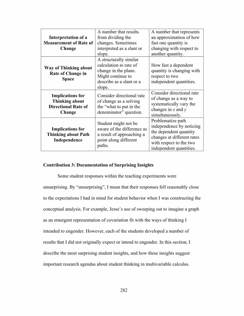
282
Interpretation of a Measurement of Rate of
Change
A number that results from dividing the changes. Sometimes interpreted as a slant or slope.
A number that represents an approximation of how fast one quantity is changing with respect to another quantity.
Way of Thinking about Rate of Change in
Space
A structurally similar calculation to rate of change in the plane. Might continue to describe as a slant or a slope.
How fast a dependent quantity is changing with respect to two independent quantities.
Implications for Thinking about
Directional Rate of Change
Consider directional rate of change as a solving the “what to put in the denominator” question.
Consider directional rate of change as a way to systematically vary the changes in x and y simultaneously.
Implications for Thinking about Path
Independence
Student might not be aware of the difference as a result of approaching a point along different paths.
Problematize path independence by noticing the dependent quantity changes at different rates with respect to the two independent quantities.
Contribution 3: Documentation of Surprising Insights
Some student responses within the teaching experiments were
unsurprising. By “unsurprising”, I mean that their responses fell reasonably close
to the expectations I had in mind for student behavior when I was constructing the
conceptual analysis. For example, Jesse’s use of sweeping out to imagine a graph
as an emergent representation of covariation fit with the ways of thinking I
intended to engender. However, each of the students developed a number of
results that I did not originally expect or intend to engender. In this section, I
describe the most surprising student insights, and how these insights suggest
important research agendas about student thinking in multivariable calculus.

283
Perspectives and sweeping out.
Jesse and Jori’s use of perspective surprised me because of the distinct
ways in which they were able to use sweeping out. Jesse’s characterization of
sweeping out from a perspective surprised me because he appeared to be able to
imagine generating a surface by flexibly switching between parameters and
variables. His use of perspective appeared to be a way to talk about cross sections,
but it was also an indication that he saw the graph as an emergent representation
of covariation. I attempted to engender the same use of perspective in Jori, and
she quickly adapted the process of sweeping out a surface. I was surprised by her
proficiency at describing the process for generating a surface in space, but came
to believe that her sweeping out process was non-quantitative. Thus, Jesse and
Jori both were proficient at sweeping out. In Jesse’s case, the surface was an
emergent representation of covariation. In Jori’s case, the surface was emergent,
but not imbued with quantitative properties. My conceptual analysis did not
explicitly attend to the possibility that one could imagine sweeping out without
imagining the surface as a representation of covariation. This insight suggests that
in future studies, I must be cognizant of both the process the student is using to
generate a function’s graph and what they understand that process to represent.
The calculus cheese and calculational reasoning.
Jori’s construction of the calculus cheese surprised me because it allowed
her to consider a non-quantitative combination of rates of change. The calculus
cheese was her way of dealing with the perceived difficulty of measuring rate of
change at a point in space. She noted that the cheese, which looked like a wedge

284
in her illustration, represented the combination of two calculus triangles. She
visualized two calculus triangles, one each from the z-x and z-y perspectives,
combining to form a wedge. This geometrical object constituted her
representation of measuring a rate of change at a point in space. I also think that
the combination of the calculus triangles, each of which implicitly measured a
rate of change, suggested to Jori it was necessary to add two separate rates of
change in measuring rate of change in space. Given this geometrical approach to
rate of change, and her accompanying calculational reasoning, I was surprised
that she was able to construct a viable measurement of rate of change in space.
She was able to characterize the “two-change” problem in addition to finding a
relationship between the changes in x and y. These results suggest that in future
studies, I must be attentive to, and prepared for engendering productive ways of
thinking in students who use calculational reasoning. My conceptual analysis in
Chapter 3 did not build on or attend to calculational reasoning, but Jori’s
responses suggest it would be productive to characterize how calculational
reasoning constrains a students’ ability to reasoning quantitatively.
Highlight points, estimation and goals.
Brian and Neil’s discussions about highlight points surprised me because
of the possible explanations for what was occurring. During the teaching
experiment, I believed that Neil could not visualize an infinite number of
“highlight points” (correspondence points), and used linear interpolation between
a finite number of highlight points to estimate the path the graph might assume.
Neil saw no need to use Brian’s process of sweeping out with an infinite number

285
of correspondence points. I now believe Neil thought his process for generating a
graph was sufficient. Neil’s major goal appeared to be to generate a graph that
mimicked Brian’s. Thus, it may not have been that he could not imagine an
infinite number of highlight points, but that Neil saw no reason to do so when
estimation produced a reasonable approximation to Brian’s graph. The possibility
that Neil was not constrained by the limits of his thinking, but by his goals for that
task, suggests that my conceptual analysis and tasks must be attentive to what the
student intends to achieve with a setting. I perceived Neil’s emphasis on a finite
number of highlight points as a constraint of his thinking, while he plausibly
could have thought in that way if he found it necessary. This result suggests that
my conceptual analyses must not only attend to a plausible way of thinking a
student might develop, but also should characterize why a student would find it
useful to think in a particular way over other methods.
The rate of change at a point in space.
Brian, and later, Neil’s, emphasis on defining the rate of change in space
surprised me because they were attending to invariance of rate of change under
direction, which requires a constant function. They were able to not only consider
rate of change in a direction in space, but a rate of change in all directions. As
they began considering rate of change in all directions, Brian broached the issue
of defining the rate of change. This exchange occurred near the end of the
teaching session, and I was not prepared to make use of his insight in the moment.
However, I believe following up on his comment could have sparked an
interesting discussion about the importance of approaching the point in space
286
from different paths. It also could have led to discussions about how to represent
the rate of change function in space. For example, suppose Brian and Neil had
proposed that the rate of change function in space could not be graphed unless
rate of change was path independent. However, suppose the rate of change
function is not invariant under direction (as is almost always the case). How then,
might they have represented direction in their construction of the rate of change
function? I cannot answer this question with data, but I predict that following up
on this discussion with students in the future could generate interesting
characterizations of thinking about path dependence and independence.
Role of tasks in eliciting surprising responses.
I was also surprised at the degree to which the tasks I used were able to
elicit utterances and actions that were productive in characterizing student
thinking. The tasks, coupled with my use of them as didactic objects, allowed the
students and I to use them as conversation pieces. For example, most of the
students continually referenced a correspondence point and sweeping out through
their entire teaching experiment. Brian and Neil made a correspondence point and
graph the central issue in thinking about two-variable functions and their rates of
change. Jesse and Jori continually referenced sweeping out and perspectives in
their teaching experiments. The tasks allowed the students to use things like
correspondence points and sweeping out to create coherence between tasks using
particular ways of thinking. In turn, I was able to document how the students
applied initial concepts in the teaching experiment to approach complex issues
about two-variable functions and their rates of change. I think that the tasks I used

287
provide an initial idea to the field of how one might gain insight into students’
ways of thinking about concepts in multivariable calculus.
In summary, I believe this dissertation has made three major contributions
to studying student thinking about two-variable functions and their rates of
change. First, I have characterized some facets of shape thinking, and the
implications of those ways of thinking for thinking about function behavior.
Second, I have described how calculational and quantitative reasoning lead to
different entailments for the meaning and construction of a function to measure
rate of change in space. Third, I have proposed how some surprising student
insights suggest important avenues of research in multivariable calculus. Finally, I
have shown how each of these contributions rely on the theoretical foundations on
which I situated this study.
Development of My Thinking
The teaching experiments and my subsequent analyses not only have made
contributions to the knowledge base of the field, but have affected my thinking.
The first four chapters of this dissertation described my thinking relative to the
instructional sequence and conceptual analysis prior to the teaching experiments,
and the data analysis chapters focused on my thinking during and between
teaching sessions. I have shown that as my thinking developed throughout the
teaching experiments and the analyses, my interpretation of students’ actions and
the resulting models of their thinking were developing simultaneously. In this
section, I consider my understanding of the literature and its constructs, my

288
thinking with regard to methodological considerations, and my thinking about
analytical method.
Literature and Constructs
Quantitative and covariational reasoning were the foundation for
conceptual analysis in chapter three, and that conceptual analysis laid the
groundwork for the didactic objects I used in the teaching sessions. My
understanding of the literature about student thinking about function and rate of
change supported that these frameworks were critical to a student’s coherent
understanding of function, but it was not until I reflected on the teaching sessions
and analyzed data in creating models of student thinking that I operationalized the
importance of these constructs in my own work.
The students’ development of “perspective” to visualize function’s graphs
emphasized the importance of quantitative reasoning. Only the expert shape
thinkers thought about a perspective as a method to generate a function’s graph.
The novice shape thinkers developed perspective as a way to “look at” the graph
as an object that was already constructed. Thus, a student’s quantitative reasoning
manifested itself in how they interpreted perspective. In general, I consider expert
shape thinking to be reliant on a high-degree of quantitative reasoning, while
novice shape thinking is reliant on non-quantitative reasoning, such as a focus on
graphs as physical objects.
My interpretation of covariational reasoning drew from Saldanha &
Thompson’s (1998) definition where one understands that two quantities are
varying in tandem and each has a value at all points in conceptual time. Their

289
work captured a great deal of the ways of thinking I was attempting to
characterize in the teaching experiments. My analyses about rate of change led me
to revisit Carlson’s (2002) framework for covariational reasoning, which focused
on how students think about how two variables vary in tandem. Carlson’s (2002)
work used Saldanha & Thompson’s (1998) image of simultaneous, continuous
variation to explain how the students in their study imagined quantities changing
in tandem using five levels of mental actions. Saldanha & Thompson’s (1998)
description of covariational reasoning helped characterize the students’ thinking
about rate of change because it allowed me to explain how an image of two or
more quantities having covaried is necessary to interpret a rate in the way I
described in my conceptual analyses.
My framework for rate of change also built upon Saldanha & Thompson’s
(1998) description of simultaneous, continuous covariation, and Thompson’s
(2011) descriptions of conceptual time. I now believe that it is not possible to
have an image of rate without an image of quantities covarying or already having
covaried. Though these descriptions were present in Thompson’s work about rate
of change, I did not fully understand why until I attempted to characterize Jori’s
thinking about rate of change.
In addition to Thompson’s work, Carlson’s (2002) framework helps
characterize the actions of my students within the study. For example, open and
closed form rate of change and calculus triangles are ways to support students in
thinking in ways consistent with MA4 and MA5 in that they help the student
imagine how one quantity changes with respect to one or more quantities over

290
intervals of conceptual time. My results also identify areas in which Carlson’s
(2002) framework could be extended to account for functions of two variables.
For example, it may be possible to extend her framework to include a description
of how a student reasons about average and instantaneous rate of change in a
direction. In this case, not only does z change with respect to x and y, but x and y
are in an invariant relationship. By nature of what her covariational reasoning
framework intended to model, Carlson did not consider how students think about
a dependent variable changing at a rate with respect to two or more independent
variables.
I situated this study within the broad research literature on function. At the
time I designed this study, I was working under the impression that these studies
more or less were evaluating a well-defined idea of students’ work and thinking
about functions. In short, my understanding of the literature was that an
understanding of function could be construed as categorical. A student
understands function, or does not. This approach led to my initial development of
frameworks that included only expert and novice shape thinking without
accounting for plausible developmental models between the two. However, I now
recognize that having a possible developmental model allows one to characterize
the student’s thinking on a continuum.
A continuum is more powerful for capturing the nuances in students’
thinking because it allows for the possibility that a student is part of more than a
single category. For example, a novice shape thinker is not thinking about
function in any classical definition because he is attending to the graph as an
291
object associated with a particular set of symbols. They attribute the graph’s
construction to a graphing calculator without understanding how the graphing
calculator generates the graph of the function. This insight came as a result of a
focus on modeling students’ ways of thinking about function, where the most
interesting and complex ways of thinking to model were when the student’s
actions indicated they did not think about function in a typical sense of the word.
As a result of this insight, my reading of the literature relative to function
now focuses on three major ideas. First, does the study define what an
understanding of function encompasses? Second, does the study attempt to
explain what the student thinks about a function, regardless of whether that way
of thinking fits the study’s definition of an understanding? Third, does the study
identify a plausible model by which the student’s understanding of function could
develop?
I believe my work contributes to exploring and clarifying what ways of
thinking about function are productive for students, as well as describing the ways
of thinking that are not productive at the moment, but nonetheless require
consideration if we desire to support students in developing the productive ways
of thinking. In general, the results of this dissertation are evidence of the
importance of quantitative and covariational reasoning.
Methodological Considerations
Initially, I conceptualized a teaching experiment as a way to experience
constraints of a student in creating a model of a student’s mathematics. While I
understood that the researcher was a necessary part of the teaching experiment, I

292
now understand that without documenting the researcher’s thinking it is nearly
impossible to trace the development of a construct within a model of student
thinking. In my case, I was not often able to have a witness present during my
teaching experiment sessions, and at best had discussions with others who
watched videotapes of the sessions. This constraint required that I document my
thinking before each session, including what I anticipated the student would do
and say based on my continuously evolving model of his or her thinking and
reflect on my hypotheses in the refinement of my model immediately after each
teaching session. In this way, I was able to track the development of each
construct in developing a model of my own thinking. This strict attention to
modeling my own thinking allowed me to make my reflections part of the data
corpus. Finding ways to attend to reflexivity by integrating the researcher’s
thinking with observations of a witness could delineate how the researcher’s
thinking contributed to each aspect of that model.
Prior to the teaching experiments, I saw microgenetic analysis as a
technique of data collection for documenting students’ actions. I now think that
microgenetic analysis can be a key component of developing a robust, viable, and
precise model of student thinking. Siegler & Crowley (1991) described the
microgenetic method as a method of studying change with three properties. First,
observations span the period from the initiation of a change to the end of a
change, marked by the stability of a system under study. Second, the density of
observations is high relative to the rate of change of the phenomenon. In short, the
rate of change of number of observations with respect to time increases if one

293
anticipates the system to be at a point of a critical change. Third, observed
behavior undergoes trial-by-trial analysis with the goal of attributing causal agents
to particular aspects of change in a system. (Siegler & Crowley, p. 606).
The microgenetic method allows one to specify the density of observations
over a period of time based on the type of change and type of complex system the
researcher is attempting to characterize. I believe the correct question in
attempting to characterize change is not how many observations over how much
time, but over what period of time to increase the density of observations. For
example, suppose that a researcher is attempting to create a mental model of a
student’s thinking as he or she participates in a two-week long instructional
sequence such as in this study. The researcher believes that the major shifts in
student’s thinking will occur on Days 1, 4 and 9 based on analysis of the
instructional sequence. Thus, the researcher might increase the density of
observations (i.e. number of documented actions, verbal cues, or gestures) on
Days 1, 4 and 9 relative to the other days in the instructional sequence. This does
not mean that the researcher takes fewer observations between these major days,
but it could suggest particularly useful days for a witness to be present. If a
witness is not able to present, these particular days, over which the greatest
change was anticipated to have occurred, could constitute a sample of video for
various witnesses to watch and discuss with the researcher.
Suppose a researcher has already conducted a number of teaching
experiments focused on a particular idea as I have in this study. I could
hypothesize when the student experiences the greatest constraint in their thinking

294
or undergoes the greatest amount of change in their actions and descriptions of
mathematical ideas. This approach could allow a researcher to systematically
focus on evaluating a particular aspect of a model of student thinking much like a
focused clinical interview. For these reasons, I believe the microgenetic method
can provide a useful complement to teaching experiment methodology in the
development of more precise and viable models of student thinking.
Future Directions
I have described how my thinking changed during the course of
conducting the teaching experiments and analyzing my data. My thinking has also
changed with regard to how I believe my work contributes to the field of
mathematics education. I think that the construct of shape thinking and my
detailed description of its facets and levels allow a more thorough characterization
of what students think about functions and their representations rather than what
they cannot do with tasks involving functions. I also think shape thinking is a first
attempt at describing what distinguishes the thinking of experts in the field from
those just learning about functions and graphs of functions. Thinking about shape
thinking as a continuum provides a preliminary framework on which subsequent
research can design tasks and instructional sequences in modeling student
thinking about functions.
I think that my descriptions of rate of change are an example of the
implications of shape thinking, and allow for further exploration into the
implications of thinking about rate of change non-quantitatively. I also think that
this study creates a base from which I can explore student thinking about total

295
derivative. In general, I see my results as both complementing and providing
specific examples of the importance of quantitative and covariational reasoning in
the context of thinking about functions and their rates of change. I am also
interested in understanding how Thompson, Castillo-Garsow, and Carlson’s
notions of conceptual time, smooth continuous variation, and a covariational
reasoning framework can build on the characterizations of student thinking I have
developed in this dissertation.
This study focused on generating models of student thinking of the four
students in the study. As I mentioned earlier, the utility and viability of the
frameworks and the constructs that compose them cannot yet extend beyond the
students who participated in this particular instructional sequence. Thus, I have
designed subsequent studies to further develop shape thinking and its many
components. I plan to focus on working with graduate students, research
mathematicians and mathematics educators to define a working limit for the
developmental trajectory in which I have situated shape thinking. I also anticipate
working with younger students as well as students entering college to define
beginning points for the developmental trajectory. While working with
mathematicians and mathematics educators, I plan to understand the ways of
thinking required to understand total derivative, which will allow me to design
subsequent teaching experiments in which I model the ways of thinking of
students as they think about rate of change in many directions. I believe that
pursuing these avenues of study will allow me to begin building this work into a
larger research program focused on multivariable functions and rate of change.

296
Chapter Summary
In this chapter, I characterized the contributions I believe my work has
made to the field of mathematics education. In doing so, I described shape
thinking as a developmental trajectory composed of novice and expert shape
thinking. I described particular ways of thinking and actions associated with those
ways of thinking for each level of the framework. Next, I proposed a framework
for students’ understanding of rate of change. I described this framework as a
continuum of ways of thinking, and situated students from the teaching
experiment session along this continuum. In this chapter, I also characterized how
my thinking changed with regard to the literature and methodology from the
study. Lastly, I considered how the development of my thinking and the
frameworks I proposed suggest some interesting directions for research.

297
REFERENCES
Akkoc, H., & Tall, D. (2003). The function concept: Comprehension and complication. British Society for Research into Learning Mathematics, 23(1).
Akkoc, H., & Tall, D. (2005). A mismatch between curriculum design and student
learning: The case of the function concept. Paper presented at the Sixth British Congress of Mathematics Education, University of Warwick.
Alson, P. (1989). Path and graphs of functions. Focus on Learning Problems in
Mathematics, 11(2), 99-106. Asiala, Brown, DeVries, Mathews, & Thomas. (1996). A framework for research
and curriculum development in undergraduate mathematics education. Research in Collegiate Mathematics Education II, 1-32.
Asiala, Cottrill, J., Dubinsky, E., & Schwingendorf, K. (1997). The development
of students' graphical understanding of the derivative. The Journal of Mathematical Behavior, 16(4), 399-431.
Bakar, M. N., & Tall, D. (1992). Students' mental prototypes for functions and
graphs. International Journal of Mathematics Education in Science and Technology, 23(1), 39-50.
Barnes, M. (1988). Understanding the function concept: Some results of
interviews with secondary and tertiary students. Research on Mathematics Education in Australia, 24-33.
Bestgen. (1980). Making and interpreting graphs and tables: Results and
implications from national assessment. Arithmetic Teacher, 28(4), 26-29. Breidenbach, D., Dubinsky, E., Hawks, J., & Nichols, D. (1992). Development of
the process conception of function. Educational Studies in Mathematics, 23, 247-285.
Carlson, M. P. (1998). A cross-sectional investigation of the development of the
function concept. In A. Schoenfeld, J. J. Kaput & E. Dubinsky (Eds.), CBMS Issues in Mathematics Education (pp. 114-162). Providence, RI: American Mathematical Society.
Carlson, M. P., Jacobs, S., Coe, E., Larsen, S., & Hsu, E. (2002). Applying
covariational reasoning while modeling dynamic events: A framework and a study. Journal for Research in Mathematics Education, 33(5), 352-378.

298
Carlson, M. P., Larsen, S., & Jacobs, S. (2001). An investigation of covariational reasoning and its role in learning the concepts of limit and accumulation Proceedings of the Twenty-third Annual Meeting of the North American Chapter of the International Group for the Psychology of Mathematics Education (Vol. 2, pp. 517-533). Snowbird, UT.
Carlson, M. P., Oehrtman, M., & Thompson, P. (2008). Foundational reasoning
abilities that promote coherence in students' understanding of function. In M. P. Carlson & C. Rasmussen (Eds.), Making the connection: Research and practice in undergraduate mathematics (pp. 150-171). Washington, DC: Mathematical Association of America.
Carlson, M. P., Smith, N., & Persson, J. (2003). Developing and connecting
calculus students' notions of rate of change and accumulation: The fundamental theorem of calculus. In N. A. Pateman, B. J. Dougherty & J. T. Zilliox (Eds.), Psychology of Mathematics Education (Vol. 2, pp. 165-172). Honolulu, HI: University of Hawaii.
Castillo-Garsow, C. (2010). Teaching the Verhulst model: A teaching experiment
in covariational reasoning and exponential growth. doctoral dissertation. Arizona State University. Tempe, AZ.
Clement, J. (2000). Analysis of clinical interviews: Foundations and model
viability. In A. E. Kelly & R. A. Lesh (Eds.), Handbook of research design in mathematics and science education (pp. 547-589). Mahwah, NJ: Lawrence Erlbaum.
Clement, L. (2001). What do students really know about functions? Connecting
Research to Teaching, 94(9), 745-748. Confrey, J. (1988). Multiplication and splitting: Their role in understanding
exponential functions. Paper presented at the Annual Meeting of the North American Chapter for the International Group for the Psychology of Mathematics Education, Dekalb, IL.
Confrey, J., & Smith, E. (1995). Splitting, covariation, and their role in the
development of exponential functions. Educational Studies in Mathematics, 26, 66-86.
DeMarois, P. (1996). Beginning algebra students' images of the function concept.
Paper presented at the 22nd Annual AMATYC Conference, Long Beach, CA.
DeMarois, P. (1997). Functions as a core concept in developmental mathematics:
A research report. Palatine, IL: William Rainey Harper College.

299
DeMarois, P., & Tall, D. (1996). Facets and layers of the function concept. Paper presented at the XX Annual Conference for the Psychology of Mathematics Education, Valencia.
Dogan-Dunlap, H. (2007). Reasoning with metaphors and constructing an
understanding of the mathematical function concept. Paper presented at the XXXI Annual Meeting of the North American Chapter of the International Group for the Psychology of Mathematics Education, Lake Tahoe, NV.
Dreyfus, T., & Eisenberg, T. (1983). The function concept in college students:
Linearity, smoothness, and periodicity. Focus on Learning Problems in Mathematics, 5(3), 119-132.
Dubinsky, E., & Harel, G. (1992). The nature of the process conception of
function. In E. Dubinsky & G. Harel (Eds.), The Concept of Function: Aspects of Epistemology. Washington DC: Mathematical Association of America.
Dubinsky, E., & McDonald, M. (2001). APOS: A constructivist theory of learning
in undergraduate mathematics education research. In D. Holton (Ed.), The teaching and learning of mathematics at university level (pp. 273-280). Dordrecht, The Netherlands: Kluwer.
Dugdale, S., Wagner, L. J., & Kibbey, D. (1992). Visualizing polynomial
functions: New insights from an old method in a new medium. Journal of Computers in Mathematics and Science Teaching, 11(2), 123–142.
Ellis, A. (2009). Patterns, quanitities, and linear functions. Mathematics Teaching
in the Middle School, 14(8), 482-491. Goldin, G. (2000). A scientific perspective on structured, task-based interviews in
mathematics education research. In A. Kelly & R. Lesh (Eds.), Handbook of research design in mathematics and science education. Mahwah, NJ: Lawrence Erlbaum.
Habre, S., & Abboud, M. (2006). Students' conceptual understanding of a
function and its derivative in an experimental calculus course. Journal of Mathematical Behavior, 25, 57-72.
Hackworth, J. A. (1994). Calculus students' understanding of rate. Master's
Thesis. San Diego State University. San Diego, CA. Retrieved from and Available at http://pat-thompson.net/PDFversions/1994Hackworth.pdf.

300
Janvier, C. (1998). The notion of chronicle as an epistemological obstacle to the concept of function. Journal of Mathematical Behavior, 17(1), 79-103.
Kleiner, I. (1989). Evolution of the function concept: A brief survey. The College
Mathematics Journal, 20, 282-300. Leinhardt, G., Zaslavsky, O., & Stein, M. (1990). Functions, graphs, and
graphing: Tasks, learning, and teaching. Review of Educational Research, 60(1), 1-64.
Martinez-Planell, R., & Trigueros, M. (2009). Students' ideas on functions of two
variables: Domain, range, and representations. In S. Swars, D. W. Stinson & S. Lemons-Smith (Eds.), Proceedings of the 31st annual meeting of the North American Chapter of the International Group for the Psychology of Mathematics Education (pp. 73-77). Atlanta, GA: Georgia State University.
Monk, G. S. (1987). Students' understandings of functions in calculus courses. Monk, G. S. (1992a). Students' understanding of a function given by a physical
model. In E. Dubinsky & G. Harel (Eds.), The Concept of Function: Aspects of Epistemology (pp. 175-193). Washington, DC: Mathematics Association of America.
Monk, G. S. (1992b). A study of calculus students' constructions of functional
situations: The case of the shadow problem. Paper presented at the Annual Meeting of the American Educational Research Association.
Monk, G. S., & Nemirovsky, R. (1994). The case of Dan: Student construction of
a functional situation through visual attributes. CBMS Issues in Mathematics Education, 4, 139-168.
Moore, K. C. (2010). The role of quantitative reasoning in precalculus students
learning central concepts of trigonometry. doctoral dissertation. Arizona State University. Tempe, AZ.
Nemirovsky, R., & Rubin, A. (1991a). It makes sense if you think about how
graphs work. But in reality... Paper presented at the XV Annual Conference for the Psychology of Mathematics Education, Assisi, Italy.
Nemirovsky, R., & Rubin, A. (1991b). Students' tendency to assume
resemblances between a function and its derivative. Paper presented at the Annual meeting of the American Educational Research Association, Chicago.

301
Oehrtman, M., Carlson, M. P., & Thompson, P. (2008). Foundational reasoning abilities that promote coherence in students' understandings of function. In M. P. Carlson & C. Rasmussen (Eds.), Making the connection: Research and practice in undergraduate mathematics (pp. 150-171). Washington, DC: Mathematical Association of America.
Rasmussen, C. (2000). New directions in differential equations: A framework for
interpreting students' understandings and difficulties. Journal of Mathematical Behavior, 20(55-87).
Saldanha, L., & Thompson, P. (1998). Re-thinking co-variation from a
quantitative perspective: Simultaneous continuous variation. In S. B. Berensah, K. R. Dawkings, M. Blanton, W. N. Coulombe, J. Kolb, K. Norwood & L. Stiff (Eds.), Proceedings of the Twenieth Annual Meeting of the North American Chapter of the International Group for the Psychology of Mathematics Education (Vol. 1, pp. 298-303). Columbus, OH: ERIC Clearninghouse for Science, Mathematics, and Environmental Education.
Sierpinska, A. (1992). On understanding the notion of function. In E. Dubinsky &
G. Harel (Eds.), The concept of function: Aspects of epistemology and pedagogy, MAA Notes (Vol. 25, pp. 25-58): Mathematical Association of America.
Smith III, J., & Thompson, P. (2008). Quantitative reasoning and the development
of algebraic reasoning. In J. Kaput & D. Carraher (Eds.), Algebra in the Early Grades (pp. 95-132). New York, NY: Lawrence Erlbaum Associates.
Steffe, L. P., & Thompson, P. (2000). Teaching experiment methodology:
Underlying principles and essential elements. In R. Lesh & A. E. Kelly (Eds.), Research design in mathematics and science education. Mahwah, NJ: Lawrence Erlbaum Associates.
Strauss, A. L., & Corbin, J. (1998). Basics of qualitative research: Techniques
and procedures for developing grounded theory (2nd ed.). Thousand Oaks, CA: Sage.
Tall, D. (1992). The transition to advanced mathematical thinking: Functions,
limits, infinity and proof. In D. Grouws (Ed.), Handbook of Research on Mathematics Teaching and Learning (pp. 495-511). New York: Macmillan.
Tall, D. (1996). Functions and calculus. In A. Bishop, K. Clements, C. Keitel &
C. Laborde (Eds.), International Handbook of Mathematics Education,

302
Part 1 (Vol. 4, pp. 289-325). The Netherlands: Kluwer Academic Publishers.
Thompson, P. (1988). Quantitative concepts as a foundational for algebraic
reasoning: Sufficiency, necessity, and cognitive obstacles. Paper presented at the Annual Meeting of the North American Chapter for the International Group for the Psychology of Mathematics Education, Dekalb, IL.
Thompson, P. (1989). A cognitive model of quantity-based algebraic reasoning.
Paper presented at the Annual Meeting of the American Educational Research Association.
Thompson, P. (1993). Quantitative reasoning, complexity, and additive structures.
Educational Studies in Mathematics, 25(3), 165-208. Thompson, P. (1994a). The development of the concept of speed and its
relationship to concepts of rate. In G. Harel & J. Confrey (Eds.), The development of multiplicative reasoning in the learning of mathematics (pp. 179-234). Albany, NY: SUNY Press.
Thompson, P. (1994b). Images of rate and operational understanding of the
fundamental theorem of calculus. Educational Studies in Mathematics, 26, 229-274.
Thompson, P. (1994c). Students, functions, and the undergraduate curriculum.
Research in Collegiate Mathematics Education. I. Issues in Mathematics Education, 4, 21-44.
Thompson, P. (2002). Didactic objects and didactic models in radical
constructivism. In K. Gravemeijer, R. Lehrer & L. V. van Oers (Eds.), Symbolizing, Modeling, and Tool Use in Mathematics Education (pp. 191-212). The Netherlands: Kluwer.
Thompson, P. (2008). Conceptual analysis of mathematical ideas: Some
spadework at the foundation of mathematics education. In O. Figueras, J. L. Cortina, S. Alatorre, T. Rojano & A. Sepulveda (Eds.), Proceedings of the Annual Meeting of the International Group for the Psychology of Mathematics Education (Vol. Vol 4, pp. 45-64). Morelia, Mexico: PME.
Thompson, P. (2011). Quantitative reasoning and mathematical modeling. In L. L.
Hatfield, S. Chamberlain & S. Belbase (Eds.), New perspectives and directions for collaborative research in mathematics education (pp. 33-57). Laramie, WY: University of Wyoming.

303
Thompson, P., Carlson, M. P., & Silverman, J. (2007). The design of tasks in support of teachers' development of coherent mathematical meanings. Journal of Mathematics Teacher Education, 10(4-6), 415-432.
Thompson, P., & Silverman, J. (2008). The concept of accumulation in calculus.
In M. P. Carlson & C. Rasmussen (Eds.), Making the connection: Research and teaching in undergraduate mathematics education (pp. 117-131). Washington, DC: Mathematical Association of America.
Thompson, P., & Thompson, A. G. (1992). Images of rate. Paper presented at the
Annual Meeting of the American Educational Research Association, San Francisco, CA.
Trigueros, M., & Martinez-Planell, R. (2007). Visualization and abstraction:
Geometric representation of functions of two variables. Paper presented at the 29th Annual Conference of the North American Chapter of the International Group for the Psychology of Mathematics Education.
Trigueros, M., & Martinez-Planell, R. (2010). Geometrical representations in the
learning of two-variable functions. Educational Studies in Mathematics, 73, 3-19.
Vinner, S. (1983). Concept definition, concept image, and the notion of function.
International Journal of Mathematical Education in Science and Technology, 14(3), 293-305.
Vinner, S. (1992). The function concept as a prototype for problems in
mathematics learning. In E. Dubinsky & G. Harel (Eds.), The Concept of Function: Aspects of Epistemology and Pedagogy. Washington, DC: Mathematics Association of America.
Vinner, S., & Dreyfus, T. (1989). Images and definitions for the concept of
function. Journal for Research in Mathematics Education, 20(4), 356-366. Yerushalmy, M. (1997). Designing representations: Reasoning about functions of
two variables. Journal for Research in Mathematics Education, 28(4), 431-466.
Weber, E., Tallman, M., Byerley, C., & Thompson, P. (in press). Introducing
derivative via the calculus triangle. Mathematics Teacher.

304
APPENDIX A
HUMAN SUBJECTS APPROVAL LETTER

305