student guide 161-192 - altair...
TRANSCRIPT

161
Once geometry cleanup is completed (e.g. surfaces ares stitched together — no unwanted free
surface edges inside the geometry), meshing is next.
Some rules of thumb when meshing:
The mesh should look rather smooth and regular (keep in mind that the analysis is based on
your mesh and the mesh quality.
Use the simplest element type suited for the problem.
Start with a coarse mesh and understand the modeling results; then use a !ner mesh if
needed.
Try to keep mesh related uncertainites to a minimum if possible. Keep it simple as it can get
more complicated on its own.
The image above illustrates an ugly mesh. This chapter focuses on when to use 2-D elements, how to
create 2-D elements of good quality, and how to use HyperMesh to create 2-D elements.
VI 2-D Meshing
This chapter includes material from the book “Practical Finite Element Analysis”. It also has been
reviewed and has additional material added by Matthias Goelke.
162
6.1 When to Use 2-D Elements
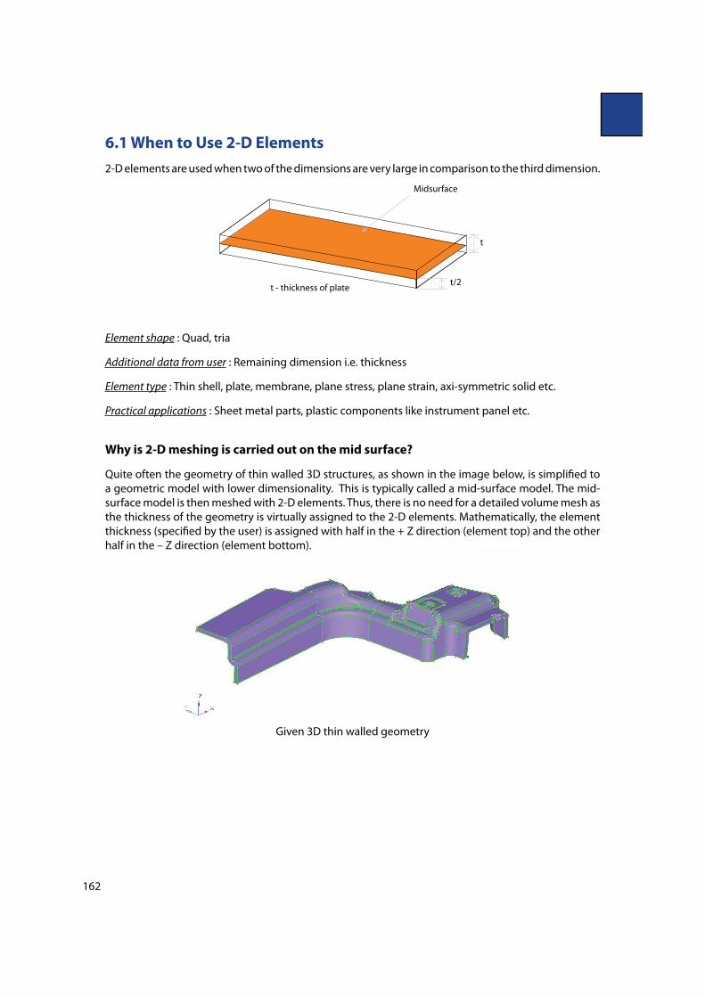
2-D elements are used when two of the dimensions are very large in comparison to the third dimension.
Midsurface
t - thickness of plate
t
t/2
Element shape : Quad, tria
Additional data from user : Remaining dimension i.e. thickness
Element type : Thin shell, plate, membrane, plane stress, plane strain, axi-symmetric solid etc.
Practical applications : Sheet metal parts, plastic components like instrument panel etc.
Why is 2-D meshing is carried out on the mid surface?
Quite often the geometry of thin walled 3D structures, as shown in the image below, is simpli!ed to
a geometric model with lower dimensionality. This is typically called a mid-surface model. The mid-
surface model is then meshed with 2-D elements. Thus, there is no need for a detailed volume mesh as
the thickness of the geometry is virtually assigned to the 2-D elements. Mathematically, the element
thickness (speci!ed by the user) is assigned with half in the + Z direction (element top) and the other
half in the – Z direction (element bottom).
Given 3D thin walled geometry

163
Derived mid-surface geometry
Enlarged view on the mid-surface model

164
2-D element shapes
Tria Quad
L(3) P(6) L(4) P(8)
Also known as
Constant Strain
Triangle (CST).
Also known as
Linear Strain
Triangle (LST)
* L – Linear element * P – Parabolic element
*( ) – Indicates number of nodes/element
Constant Strain Triangle (CST) Information
Some remarks regarding the Constant Strain Triangle (CST) element (explanation taken from:
The CST (Constant Strain Triangle) –An insidious survivor from the infancy of FEA, by R.P. Prukl, MFT
http://www.!niteelements.net/Papers/The%20CST.PDF.
The CST was the !rst element that was developed for !nite element analysis (FEA) and 40-50
years ago it served its purpose well. In the meantime, more accurate elements have been
created and these should be used to replace the CST.
The Explanation
Consider a 3-noded plane stress element in the xy-plane with node points 1, 2 and
3. The x-de"ections are u1, u2, u3 and the y-de"ections v1, v2 and v3, totalling six values
altogether.
The displacement function then has the following form (using six constants i to describe the
behaviour of the element):
The direct strains can then be calculated by di#erentiation:

165
What does this mean?
The strains in such an element are constants. We know, however, that in a beam we have compression
at the top and tension at the bottom. Our single element is, therefore, not capable of modelling
bending behaviour of a beam, it cannot model anything at all. Note: Three-noded elements for other
applications than plane stress and strain are quite acceptable, e.g., plate bending and heat transfer.
The Remedy
Use elements with four nodes. We then have eight constants to describe the behaviour of the element:
The direct strains are then as follows:
The strain in the x-direction is now a linear function of its y-value. This is much better than for the
triangular element. Use triangular elements which also include the rotational degree of freedom
about the z-axis normal to the xy-plane.

166
6.2 Family of 2-D Elements
1) Plane stress :
Degrees of Freedom (DOFs) – 2 / node {Ux , U
y (in-plane translations)}
Stress in z direction (thickness) is zero(σz = 0)
167
y
zx
Total dof = 8
Uy
Ux
Uy
Ux
Uy
Ux
Uy
Ux
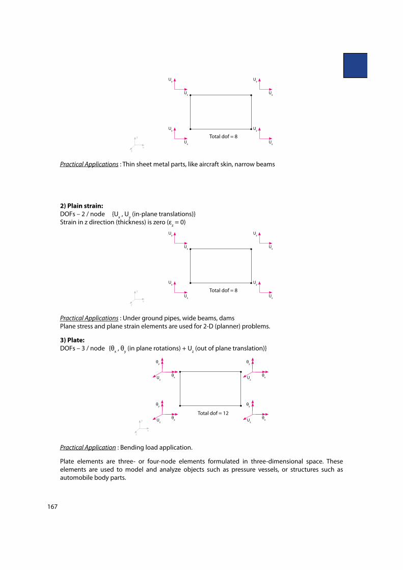
Practical Applications : Thin sheet metal parts, like aircraft skin, narrow beams
2) Plain strain:
DOFs – 2 / node {Ux , U
y (in-plane translations)}
Strain in z direction (thickness) is zero (εz = 0)
y
zx
Total dof = 8
Uy
Ux
Uy
Ux
Uy
Ux
Uy
Ux
Practical Applications : Under ground pipes, wide beams, dams
Plane stress and plane strain elements are used for 2-D (planner) problems.
3) Plate:
DOFs – 3 / node {θx , θ
y (in plane rotations) + U
z (out of plane translation)}
Total dof = 12
y
zx
θy
θxU
z
θy
θxU
z
θy
θxU
z
θy
θxU
z
Practical Application : Bending load application.
Plate elements are three- or four-node elements formulated in three-dimensional space. These
elements are used to model and analyze objects such as pressure vessels, or structures such as
automobile body parts.

168
The out-of-plane rotational DOF is not considered for plate elements. You can apply the other
rotational DOFs and all the translational DOFs as needed.
Nodal forces, nodal moments (except when about an axis normal to the element face), pressures
(normal to the element face), acceleration/gravity, centrifugal and thermal loads are supported.
Surface-based loads (pressure, surface force, and so on, but not constraints) and element properties
(thickness, element normal coordinate, and so on) are applied to an entire plate element. Since these
items are based on the surface number of the lines forming the element, and since each element
could be composed of lines on four di#erent surface numbers, how these items are applied depend
on whether the mesh is created automatically (by either the mesher from a CAD model or the 2D
mesh generation), or whether the mesh is created by hand. The surface number of the individual lines
that form an element are combined as indicated in the table above to create a surface number for the
whole element. Loads and properties are then applied to the entire element based on the element’s
surface number
4) Membrane :
DOFs – 3 / node {Ux , U
y (in plane translations) + θ
z (out of plane rotation)}
Total dof = 12
y
zx
Uy
Uxθ
z
Uy
Uxθ
z
Uy
Uxθ
z
Uy
Uxθ
z
Practical Application: Balloon, Ba<es
5) Thin shell :
Thin shell elements are the most general type of element.
DOFs : 6 dof / node ( Ux , U
y , U
z , θ
x , θ
y , θ
z).
Thin Shell = Plate + Membrane
( Ux , U
y , U
z , θ
x , θ
y , θ
z) = U
z , θ
x , θ
y + U
x , U
y , θ
z
(3T+3R) = (1T+2R) + (2T+1R)

169
Total dof = 24
y
zx
Uyθ
y
Uxθ
xU
zθ
z
Uyθ
y
Uxθ
xU
zθ
z
Uyθ
y
Uxθ
xU
zθ
z
Uyθ
y
Uxθ
xU
zθ
z
Practical Application : Thin shell elements are the most commonly used elements.
6) Axisymmetric Solid :
DOFs - 2 / node {Ux , U
z (2 in plane translations, Z axis is axis of rotation)}
Why is the word ‘solid’ in the name of a 2-D element? This is because though the elements are planner,
they actually represent a solid. When generating a cylinder in CAD software, we de!ne an axis of
rotation and a rectangular cross section. Similarly, for an axi-symmetric model we need to de!ne an
axis of rotation and a cross section (planer mesh). The 2-D planer mesh is mathematically equivalent
to the 3-D cylinder.
y
zx
Total dof = 8
Uy
Ux
Uy
Ux
Uy
Ux
Uy
Ux
Practical Applications : Pressure vessels, objects of revolutions subjected to axi-symmetric boundary
conditions
6.3 Thin Shell Elements
In the following we investigate the “performance” of quad and tria-elements by looking at a plate with
a circular hole. The modeling results are then compared with a given analytical answer.

170
10,000 N
10 mm thick
Ф 50
1000
1000
Analytical answer :
The Stress Concentration Factor (SCF) is de!ned as = max. stress / nominal stress
In this example the nominal stress is = F/A = 10,000 N/(1000 mm*10 mm) =1 N/mm2
For an ini!nite plate SCF =3
Hence, the maximum stress = Stress Concentration Factor (SCF) * nominal stress = 3 N/mm2
In the !rst part of this study the e#ects of element type (quad versus tria elements) on the modeling
results are investigated. The global mesh size is 100.
The boundary conditions for all models are the same: the translational degrees of freedom (x-, y-,
z- displacements=0) of all nodes along the left edge of the model are constrained (green symbols)
whereas the nodes along the right edge are subjected to forces in the x-direction (total magnitude
10.000 N).

171
In order to better control the mesh pattern surrounding the hole, two so called “washers” have
been introduced (i.e. the initial surface is trimmed by two circles with a radii of 45 mm and 84 mm,
respectively.
In the stress contour plots shown below, the maximum principal stress is depicted, respectively.
Note that by default the element stresses for shell (and solid elements) are output at the element
center only. In other words, these stresses are not exactly the ones “existing” at the hole. To better
resolve the stresses at the hole, the element stresses are output at the grid points using bilinear
extrapolation (in HyperMesh activate the Control cards > Global output request > Stress >
Location: Corner).
E!ect of Element Type (quads vs. trias)
Model 1: The hole is meshed with 16 tria elements. The maximum principal stress (corner location) is
2.32 N/mm2 (the analytical result is 3 N/mm2).

172
Model 2: The hole is meshed with 16 quad elements. The maximum principal stress (corner location)
is 2.47 N/mm2 (the analytical result is 3 N/mm2).
Despite the fact, that both results di#er signi!cantly from the analytical reference value of 3 N/mm2,
it is apparent that the quad elements (17 % error) are “better” than tria elements (23 % error). All in
all, both models are inappropriate when it comes to quantitatively assessing the stresses at the hole.
Moreover, another even more important lesson to be learned is that the FEM program does not tell
you that the mesh is inacceptable – this decision is up to the CAE engineer
E!ect of Mesh Density
In the following the e#ect of element size, i.e. number of elements at the hole, on the modeling
results is discussed.
173
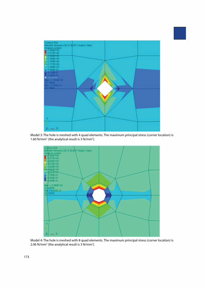
Model 3: The hole is meshed with 4 quad elements. The maximum principal stress (corner location) is
1.60 N/mm2 (the analytical result is 3 N/mm2).
Model 4: The hole is meshed with 8 quad elements. The maximum principal stress (corner location) is
2.06 N/mm2 (the analytical result is 3 N/mm2).
174
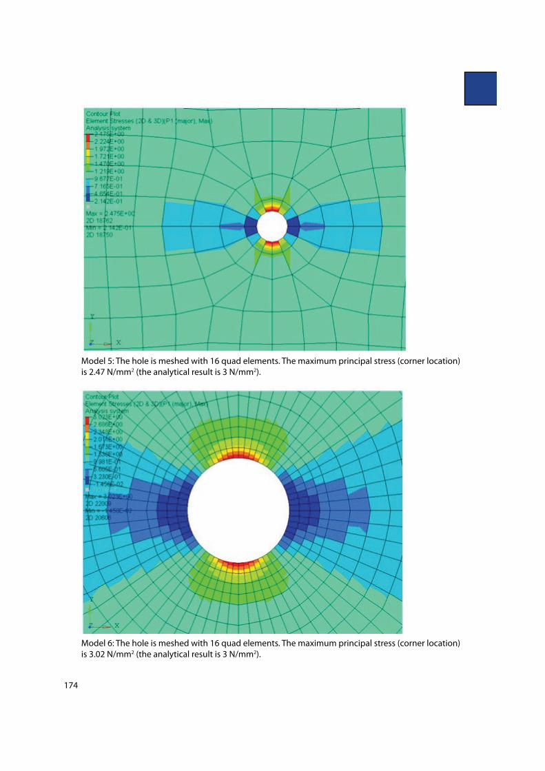
Model 5: The hole is meshed with 16 quad elements. The maximum principal stress (corner location)
is 2.47 N/mm2 (the analytical result is 3 N/mm2).
Model 6: The hole is meshed with 16 quad elements. The maximum principal stress (corner location)
is 3.02 N/mm2 (the analytical result is 3 N/mm2).
175
Element Type # Elements at Hole Stress (N/mm2)
(corner location)
Model 1 Tria 16 2.32
Model 2 Quad 16 2.47
Model 3 Quad 4 1.6
Model 4 Quad 8 2.0
Model 5 Quad 16 2.47
Model 6 Quad 64 3.02
Conclusion:
The conclusion from the !rst exercise was that quad elements are better than
triangular elements. As indicated by the results shown before: the greater the
number of elements in the critical region (i.e. hole), the better its accuracy.
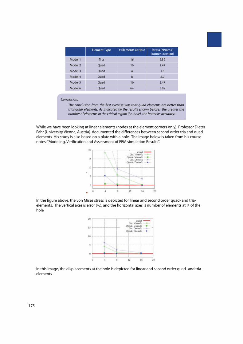
While we have been looking at linear elements (nodes at the element corners only), Professor Dieter
Pahr (University Vienna, Austria). documented the di#erences between second order tria and quad
elements His study is also based on a plate with a hole. The image below is taken from his course
notes: “Modeling, Veri!cation and Assessment of FEM simulation Results”.
In the !gure above, the von Mises stress is depicted for linear and second order quad- and tria-
elements. The vertical axes is error (%), and the horizontal axes is number of elements at ¼ of the
hole
In this image, the displacements at the hole is depicted for linear and second order quad- and tria-
elements
176
Conclusion:
Second order quad elements behave/perfom best, whereas linear trias are
“problematic”. These element related e"ects are less severe while looking at
displacements (nodal results).
If this is so, then why not always create a very !ne mesh with the maximum possible number of
nodes and elements? Why is the usual guideline for meshing 12-16 elements around holes in
critical areas?
The reason is because the solution time is directly proportional to the (dof )2. Also large size models
are not easy to handle on the computer due to graphics card memory limitations. Analysts have to
maintain a !ne balance between the level of accuracy and the element size (dof ) that can be handled
satisfactorily with the available hardware con!guration.
How are thumb rules made?
Usually we get instructions from the client about a speci!c number of elements to use on a hole or
!llet, a speci!c mesh pattern for bolted welded joints, etc. How do they decide these rules?
It is based on a simple exercise like the one above. The results of di#erent mesh con!gurations
are compared with a known analytical answer and the one which gives the logical accuracy with a
reasonable solution time is selected.
Most of the industries follow the following thumb rule for the number of elements on holes:
Minimum number of elements :
critical areas = 12
general areas = 6
6.4 E!ect of Biasing in the Critical Region
15
1
No Bias Bias 15 at the right edge
During meshing, an option named “biasing” may be used. In our day to day life, we use the word
bias the following way, “My boss is biased, he prefers my colleague even though both of us have
equal quali!cation and eXciency”. In the same manner, when element length is not the same on
the edge and biased towards a point, then it is known as biased meshing. Di#erent commercial
software calculate bias di#erently. One of the simplest schemes is where the bias factor is a ratio of
the maximum element length divided by the minimum element length.

177
No bias bias 5 bias 20
The above geometry was split along the diagonal and the bias was de!ned on the diagonals (at the
edge point near the circular hole).
6
6
6 6
6 6
6 6
6 66
6
Biased Mesh Exercise :
Distribution of elements
Stress N/mm2
(exact answer 3 N/mm2)
Nodes Elements
No Bias 1.59 168 144
Bias 5 2.13 168 144
Bias 10 2.41 168 144
Bias 15 2.56 168 144
Bias 20 2.65 168 144
The conclusion from the previous example was that the higher the number of elements in the critical
area, the higher the accuracy. The example on biasing shows that even without increasing the
number of elements, one can achieve a better result just by the appropriate arrangement of the nodes
and elements. This was done at no extra computational cost.
6.5 Symmetric Boundary Conditions
In order to reduce the total number of elements one may consider only 1/2 or 1/4 of the original
structure. In this way a locally re!ned mesh (i.e. higher acuracy) may be used whereas the total number
of elements may still be less than an evenly coarse meshed full model.

178
Full Plate:
Ux U
y U
z θ
x θ
y θ
z
(123456)= 0
Force = 10,000 N
y
zx
Half Plate:
Vertical edge
restraint:
Ux U
y U
z θ
x θ
y θ
z
(123456)= 0
Force = 5,000 N
Horizontal edge restraint: Uy θ
x θ
z (246)= 0
y
zx
How to apply symmetric boundary conditions :
Step 1 : Write plane of symmetry for half plate i.e. x z
Step 2 : Fix in plane rotations (θx , θ
z) and out of plane translations (U
y).
Please !nd ore details about symmertic boundary conditions in Chapter 10.
Stress Displacement Nodes Elements
Complete model 2.68 0.00486 352 320
Half Symmetry 2.68 0.00486 187 160
The advantage of symmetric boundary conditions is that the same accuracy is achieved at a lesser
computational time and cost.
Symmetric boundary conditions should not be used for dynamic analysis (vibration analysis). It can
not calculate anti nodes.

179
6.6 Di!erent Element Type Options for Shell Meshing
1) Pure quad elements
2) Mixed mode
3) Equilateral tria
4) (Right angle) R-tria
The image above shows a geometry that has been partially meshed. How would you “link” both
meshes? Depending on whether some single tria elements are allowed, you may use the mixed
meshing method or the pure quad mesh. Both meshes are shown below. Note the more homogenoues
mesh pattern resulting from “mixed” meshing.
Mixed Mesh Quad Only Mesh
The mixed mode element type is the most common element type used due to the better mesh pattern
that it produces (restriction : total tria % <5). Sometimes for structural analysis or for convergence and
better results for a non linear analysis, the pure quadrilateral element meshing option is selected.
If quads are better than trias, why not always mesh using only quad elements? Why do FEA
software provide the option for tria elements?

180
1) Mesh transition: In structural and fatigue analysis, rather than a uniform mesh, what helps is a small
element size in the critical areas and a coarse mesh or bigger elements in general areas. This type of
mesh gives good accuracy with manageable dofs. Trias help in creating a smooth mesh transition
from a dense mesh to a coarse mesh.
2 ) Complex geometry: Geometry features like rib ends or sharp cutouts demand for the use of triangular
elements. If quads are used instead of trias, then it will result in poor quality elements.
3) Better mesh #ow: For crash or non linear analysis, systematic mesh "ow lines where all the elements
satisfy the required quality parameters is very important. Using a mix-mode element type instead of
pure quad element type helps to achieve better "ow lines and convergence of solution.
4) Tetra meshing (conversion from Tria to Tetra): For tetra meshing, all the outer surfaces are meshed
using 2-D triangular elements and then trias are converted to tetras. This methodology is discussed
in detail in the next chapter.
5) Mold #ow analysis : Mold "ow analysis requires triangular elements.
Comparison between Equilateral tria and Right angle tria meshing.
The default tria mesh in commercial software produce equilateral triangles while the R-tria option
generates right angle triangles (generating a rectangular or square mesh and then splitting along the
diagonal gives two trias per element).
In the !gure above, the left image shows meshing with equilateral trias, while the right image shows
meshing with the option R-trias (which simply splits quad elements into two tria elements).
The ideal shape for a triangular element is an equilateral triangle and is theoretically better than a
R-tria element. But for the following speci!c applications, R-trias have an advantage over equilateral
trias.
1) Tetra meshing :
For de!ning contacts, a similar mesh pattern on the two surfaces is desirable. The equilateral tria
option produces a ziz-zag mesh and there is also no control over the mesh pattern. A similar mesh
requirement could be achieved by generating a structured quadrilateral mesh (maintaining exactly

181
same number of elements on two contact surfaces) and then splitting it to trias (R-tria). Typical
applications are as follows:
a) Bolt hole and washer area:
b) Bearing contact surfaces: Contact surfaces are meshed with quad elements (same mesh pattern
and equal number of elements) and converted to trias before tetra conversion.

182
2) Variable thickness of ribs for mold "ow analysis
The ribs are modelled using quad elements in three layers as shown below and then split to R-trias.
The average section thickness is assigned to each di#erent layer.
t1avg
= 1.5 mm
t3avg
= 3.5 mm
t2avg
= 2.5 mm
1 mm
2 mm
3 mm
4 mm
6.7 Geometry Associative Mesh
Creating a geometry associative mesh allows for automatic meshing to be carried out by picking
surfaces or volumes from the geometry. The generated mesh is associative with the geometry.
Advantages :
1) If the geometry is changed, then the mesh will also change automatically.
2) Boundary conditions could be applied on the geometry (edges, surfaces instead of nodes and
elements, etc.) which is more user friendly.
183
Original geomtery Geometry based mesh
Geometry modi!cation
(cut hole at the center)
Auto update of mesh
6.8 How Not to Mesh
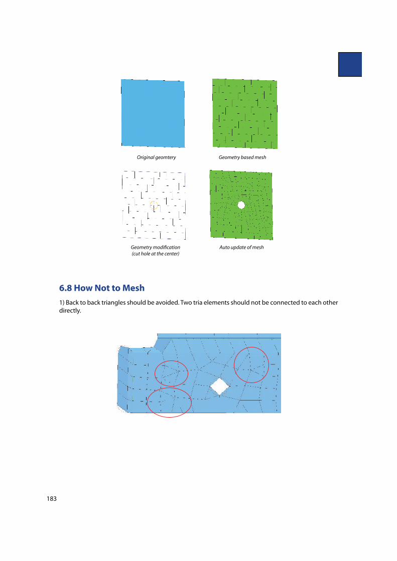
1) Back to back triangles should be avoided. Two tria elements should not be connected to each other
directly.

184
2) On plane surfaces triangular element should be avoided.
not recommended not recommended recommended
3) No mesh transition on constant radius !llets / curvatures
The mesh transition should be carried out on the planer surfaces
4) Avoid tria elements on outer edges or holes

185
5) What is not acceptable at a professional level
Nodes = 1400, Elements = 1309
Not acceptable
Nodes = 1073, Elements = 982
What they expected at a professional level
6) Circular holes should be modelled carefully with a washer (1.5 to 2 times diameter) and a minimum
of two layers around the hole.

186
7) Holes should be modelled with an even number of equally spaced elements:
For a better representation of the hole geometry and smooth mesh "ow lines, holes should be
modelled with an even number of elements (like 6, 8, 12,16 etc. rather than 5, 7, 9 or 13).
7 elements on hole (odd number),
not recommended
8) Nodes should lie properly on the surface, with no deviation (and no kinks).
Switch o# the element mesh lines and observe the contour (in particular at curvatures). Kinks as
shown above are not acceptable.
9) Follow the feature lines (nodes should lie exactly on the edges).

187
10) Instead of a zig-zag distribution, a structured or smooth mesh is recommended (nodes aligned in
a straight line)
not recommended recommended
Use of a“smooth” option, provided by most of the commercial software, helps in achieving systematic
mesh.
11) For crash analysis, follow the mesh "ow line requirement.
Diamond elements are not
allowed
12) For crash analysis, rotating quads are not allowed.
Rotating quads recommended
Recommended for structural analysis
Not recommended for crash analysis
Recommended for crash analysis
Not recommended for structural analysis

188
13) For Crash analysis, constant mesh size (by using trias) is preferred (due to a minimum element
length and a time step criteria).
Recommended for crash analysis
Variable mesh size not recommended for crash but recommended for structural analysis
6.9 Creating 2-D Elements in HyperMesh
A surface mesh or “shell mesh” represents model parts that are relatively two-dimensional, such as
sheet metal or a hollow plastic cowl or case. In addition, surface meshes placed on the outer faces
of solid objects are used as a baseline mapping point when creating more complex 3-D meshes (the
quality of a 3-D mesh largely depends on the quality of the 2-D mesh from which it is generated).
Three-noded trias, four-noded quads, six-noded trias, and eight-noded quads can all be built in
HyperMesh. These two-dimensional elements can be built in any of the following panels. A detailed
look at automeshing and shrink wrap meshing will follow. For additional information regarding the
other panels, please refer to the appropriate video.
Below is a listing of the panels available for creating and editing 2-D elements. Most of these tools
are located in the menu bar by selecting Mesh > Create > 2D Elements.
automesh: Builds elements on surfaces according to user speci!cations (further details
given below).
shrink wrap: Builds 2-D (optionally 3-D) simpli!ed meshes of existing complex models
further details are given below and in Chapter 7 3D Meshing).
cones: Builds elements on conic or cylindrical surfaces.
drag: Builds elements by dragging a line, row of nodes, or group of elements along a vector.
edit element: Builds elements by hand.
6.9 Creating 2-D Elements in HyperMesh

189
elem o"set: Builds elements by o#setting a group of elements in the direction of their
normals.
line drag: Builds elements by dragging a line or group of elements along or about a control
line.
planes: Builds elements on square or trimmed planar surfaces.
ruled: Builds elements between two rows of nodes, a row of nodes and a line, or two lines.
spheres: Builds elements on spherical surfaces.
spin: Builds elements by spinning a line, row of nodes, or group of elements about a vector.
spline: Builds elements that lie on a surface de!ned by lines.
torus: Builds elements on toroidal surfaces
Automeshing
The Automesh panel is a key meshing tool in HyperMesh. Its meshing module allows you to specify
and control element size, density, type, and node spacing, and also perform quality checks before
accepting the !nal mesh.
The optimal starting point for creating a shell mesh for a part is to have geometry surfaces de!ning
the part. The most eXcient method for creating a mesh representing the part includes using the
Automesh panel and creating a mesh directly on the part’s surfaces. The Automesh panel can be
accessed from the menu bar by selecing Mesh > Create > 2D AutoMesh. A part can be meshed all
at once or in portions. To mesh a part all at once, it may be advantageous to !rst perform geometry
cleanup (please see Chapter 3 on Geometry) of the surfaces, which can be done in HyperMesh.
Automeshing

190
Provided your geometry is clean e.g. the surface of the rib is merged with the adjacent
surfaces, then the resulting mesh will be automatically compatible (all elements are
connected with each other).
There are two approaches to the Automesh panel, depending on whether or not you use
surfaces as the basis for the operation.
1. If you use surfaces, you may choose from a greater variety of algorithms, have more
"exibility in specifying the algorithm parameters, and employ the mesh-smoothing
operation to improve element quality.
2. If you do not use surfaces, the meshing process is usually faster and uses less memory. Most
of the functions are still available and operate in the same way. Furthermore, there are
situations in which it is not possible or not desirable to create a surface.
For either method, the module operates the same. You interactively control the number of elements
on each edge or side and can determine immediately the nodes that are used to create the
mesh. You can adjust the node biasing on each edge to force more elements to be created near one
end than near the other, which allows you to see immediately the locations of the new nodes.
You can also specify whether the new elements should be quads, trias, or mixed and whether they
should be !rst or second order elements.

191
The created mesh can also be previewed, which allows you to evaluate it for element quality before
choosing to store it in the HyperMesh database. While you are in the meshing module, you can use
any of viewing tools on the Visualization toolbar to simplify the visualization of complex structures
in your model.
If you use surfaces, you can specify the mesh generation and visualization options to use on each
individual surface. You may choose from several mesh generation algorithms. Mesh smoothing is
also available and you may select the algorithm for that operation as well.
To learn more about some of the 2 D Automeshing options available in HyperMesh, please view the
interactive video “Starter_2D_meshing.htm” (no HW installation required)
What you need to know/remember:
While working with the Automesh panel you will come across the following options and settings:
Element size = the element size in the model may deviate from the speci!ed size considerably (it
depends on the size of the surface).
Mesh type = mixed; default (is a combination of many quad-shaped elements and some tria
elements). Leads to rather smooth meshes.
Elems to surf comp vs. Elems to current comp = speci!es the “storage“ place of the elements.
Start meshing, explore the meaning of the other settings latter! What may happen is that the mesh
looks a bit weird …
Some surfaces apparently cause trouble. This may not actually be a problem, but a matter of your
visual settings. In this example, the geometry is still shaded, overprinting the mesh in some spots.
Displaying the geometry in wireframe and shading the elements will improve the mesh “visibility“.

192
Note: In case you don‘t see any mesh, check the Model Browser and the status of the corresponding
collector (is the elem icon activated?)
Shrink Wrap Meshing
Shrink wrap meshing is a method to create a simpli!ed mesh of a complex model when high-
precision models are not necessary, as is the case for powertrain components during crash
analysis. The model’s size, mass, and general shape remains, but the surface features and details
are simpli!ed, which can result in faster analysis computation. You can determine the level of detail
retained by determining the mesh size to use, among other options.
You can shrink wrap elements, components, surfaces, or solids.
The shrink wrap allows for wrapping of multiple components if they are selected.
The selection provides the option to wrap all elements, components, surfaces or solids,
or only a certain portion of the model if desired. The input to the shrink wrap (that is, the
model parts that you wish to wrap) can consist of 2-D or 3-D elements along with surfaces
or solids.
A shrink wrap mesh can be generated as a surface mesh (using a loose or tight wrapping), or as a
full-volume hex mesh by use of the Shrink Wrap panel. This panel is located in the menu bar by
selecting Mesh > Create > Shrink Wrap Mesh. The distinction between surface or volume mesh is
an option labeled generate solid mesh. The Shrink Wrap panel is covered in more detail in the 3-D
meshing section.
Shrink Wrap Meshing