Stuck between a rock and a reflection: A tutorial on low-frequency modelsfor seismic inversion

Mark Sams1 and David Carter2

Abstract

Predicting the low-frequency component to be used for seismic inversion to absolute elastic rock propertiesis often problematic. The most common technique is to interpolate well data within a structural framework. Thisworkflow is very often not appropriate because it is too dependent on the number and distribution of wells andthe interpolation algorithm chosen. The inclusion of seismic velocity information can reduce prediction error,but it more often introduces additional uncertainties because seismic velocities are often unreliable and requireconditioning, calibration to wells, and conversion to S-velocity and density. Alternative techniques exist that relyon the information from within the seismic bandwidth to predict the variations below the seismic bandwidth;for example, using an interpretation of relative properties to update the low-frequency model. Such methodscan provide improved predictions, especially when constrained by a conceptual geologic model and knownrock-physics relationships, but they clearly have limitations. On the other hand, interpretation of relative elasticproperties can be equally challenging and therefore interpreters may find themselves stuck — unsure how tointerpret relative properties and seemingly unable to construct a useful low-frequency model. There is no im-mediate solution to this dilemma; however, it is clear that low-frequency models should not be a fixed input toseismic inversion, but low-frequency model building should be considered as a means to interpret relative elas-tic properties from inversion.

IntroductionInversion of seismic reflection data to elastic imped-

ances can add significant value to seismic reservoir char-acterization. The benefits of inversion are well-known(e.g., Latimer et al., 2000): increased resolution, conver-sion from an interface to a layer property, conversion tophysical rock properties (impedances), removal of thewavelet, and reduced tuning, all of which lead to animproved interpretability of the seismic data in a quali-tative and a quantitative sense. Many of these advantagesare dependent on the integration of an accurate low-fre-quency model with band-limited seismic data to producethe absolute impedances. Most deterministic inversionalgorithms operate in the absolute elastic domain andrequire an estimate of the absolute elastic propertiesthroughout the volume prior to inversion. These volumesof absolute properties are used in various ways depend-ing on the inversion algorithm chosen. They can act asstarting models, in which case they may contain a broadrange of frequencies, or they can act as low-frequencymodels that supply data and constraints below the band-width of the seismic data. Absolute values are also oftenused to supply additional inversion constraints based oninterrelationships between the different properties being

determined (e.g., acoustic impedance to shear imped-ance and acoustic impedance to density, so called rock-physics constraints), and they can be used as hard con-straints, for example, ensuring that Poisson’s ratio liesbetween zero and 0.5. In practice, the results of inversionto absolute properties are supplemented with relativeproperties, which are commonly the result of applying aband-pass filter to the absolute properties. The seismicreflection data, relative impedances, and absolute imped-ances should all be considered during interpretation toensure that conclusions are not being incorrectly influ-enced by the low-frequency models, although there aremany examples in the literature in which this does notseem to be the case. The concern about absolute imped-ances is due to the difficulty of providing reasonable low-frequency models and the potential that they can nega-tively bias the absolute estimates and produce incorrectinterpretations. Ball et al. (2015) show that with certainassumptions, no low-frequency model is required for in-version to relative impedances when they are appropri-ately defined (Ball et al., 2014). As such, there is anargument for excluding low-frequency models and rely-ing only on the relative properties for interpretation. Onthe other hand, the problem with relative impedances is

1Ikon Science, Kuala Lumpur, Malaysia. E-mail: msams@ikonscience.com.2KrisEnergy (Gulf of Thailand) Ltd., Bangkok, Thailand. E-mail: david.carter@krisenergy.com.Manuscript received by the Editor 18 September 2016; revisedmanuscript received 4 December 2016; published online 21March 2017. This paper

appears in Interpretation, Vol. 5, No. 2 (May 2017); p. B17–B27, 9 FIGS.http://dx.doi.org/10.1190/INT-2016-0150.1. © 2017 Society of Exploration Geophysicists and American Association of Petroleum Geologists. All rights reserved.

t

Tools, techniques, and tutorials

Interpretation / May 2017 B17Interpretation / May 2017 B17

Dow

nloa

ded

05/0

8/17

to 2

11.2

5.15

.114

. Red

istr

ibut

ion

subj

ect t

o SE

G li

cens

e or

cop

yrig

ht; s

ee T

erm

s of

Use

at h

ttp://

libra

ry.s

eg.o

rg/

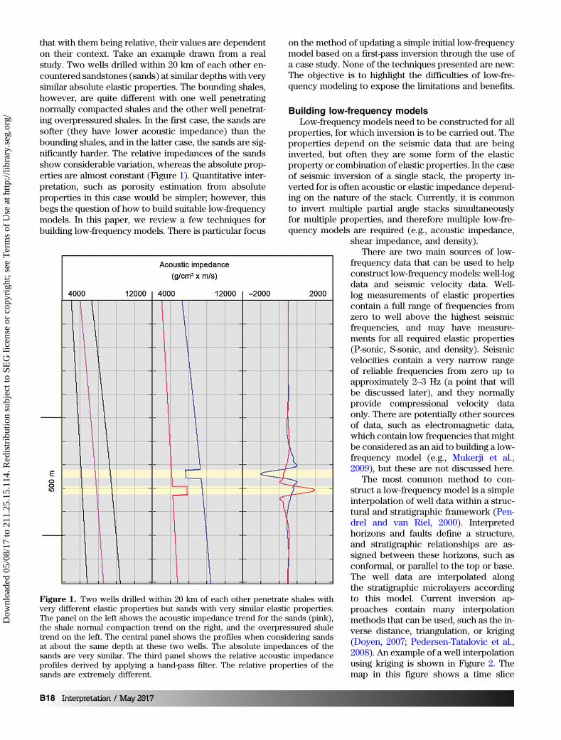
that with them being relative, their values are dependenton their context. Take an example drawn from a realstudy. Two wells drilled within 20 km of each other en-countered sandstones (sands) at similar depths with verysimilar absolute elastic properties. The bounding shales,however, are quite different with one well penetratingnormally compacted shales and the other well penetrat-ing overpressured shales. In the first case, the sands aresofter (they have lower acoustic impedance) than thebounding shales, and in the latter case, the sands are sig-nificantly harder. The relative impedances of the sandsshow considerable variation, whereas the absolute prop-erties are almost constant (Figure 1). Quantitative inter-pretation, such as porosity estimation from absoluteproperties in this case would be simpler; however, thisbegs the question of how to build suitable low-frequencymodels. In this paper, we review a few techniques forbuilding low-frequency models. There is particular focus

on the method of updating a simple initial low-frequencymodel based on a first-pass inversion through the use ofa case study. None of the techniques presented are new:The objective is to highlight the difficulties of low-fre-quency modeling to expose the limitations and benefits.

Building low-frequency modelsLow-frequency models need to be constructed for all

properties, for which inversion is to be carried out. Theproperties depend on the seismic data that are beinginverted, but often they are some form of the elasticproperty or combination of elastic properties. In the caseof seismic inversion of a single stack, the property in-verted for is often acoustic or elastic impedance depend-ing on the nature of the stack. Currently, it is commonto invert multiple partial angle stacks simultaneouslyfor multiple properties, and therefore multiple low-fre-quency models are required (e.g., acoustic impedance,

shear impedance, and density).There are two main sources of low-

frequency data that can be used to helpconstruct low-frequencymodels: well-logdata and seismic velocity data. Well-log measurements of elastic propertiescontain a full range of frequencies fromzero to well above the highest seismicfrequencies, and may have measure-ments for all required elastic properties(P-sonic, S-sonic, and density). Seismicvelocities contain a very narrow rangeof reliable frequencies from zero up toapproximately 2–3 Hz (a point that willbe discussed later), and they normallyprovide compressional velocity dataonly. There are potentially other sourcesof data, such as electromagnetic data,which contain low frequencies that mightbe considered as an aid to building a low-frequency model (e.g., Mukerji et al.,2009), but these are not discussed here.

The most common method to con-struct a low-frequency model is a simpleinterpolation of well data within a struc-tural and stratigraphic framework (Pen-drel and van Riel, 2000). Interpretedhorizons and faults define a structure,and stratigraphic relationships are as-signed between these horizons, such asconformal, or parallel to the top or base.The well data are interpolated alongthe stratigraphic microlayers accordingto this model. Current inversion ap-proaches contain many interpolationmethods that can be used, such as the in-verse distance, triangulation, or kriging(Doyen, 2007; Pedersen-Tatalovic et al.,2008). An example of a well interpolationusing kriging is shown in Figure 2. Themap in this figure shows a time slice

Figure 1. Two wells drilled within 20 km of each other penetrate shales withvery different elastic properties but sands with very similar elastic properties.The panel on the left shows the acoustic impedance trend for the sands (pink),the shale normal compaction trend on the right, and the overpressured shaletrend on the left. The central panel shows the profiles when considering sandsat about the same depth at these two wells. The absolute impedances of thesands are very similar. The third panel shows the relative acoustic impedanceprofiles derived by applying a band-pass filter. The relative properties of thesands are extremely different.

B18 Interpretation / May 2017

Dow

nloa

ded

05/0

8/17

to 2

11.2

5.15

.114

. Red

istr

ibut

ion

subj

ect t

o SE

G li

cens

e or

cop

yrig

ht; s

ee T

erm

s of

Use

at h

ttp://

libra

ry.s

eg.o

rg/

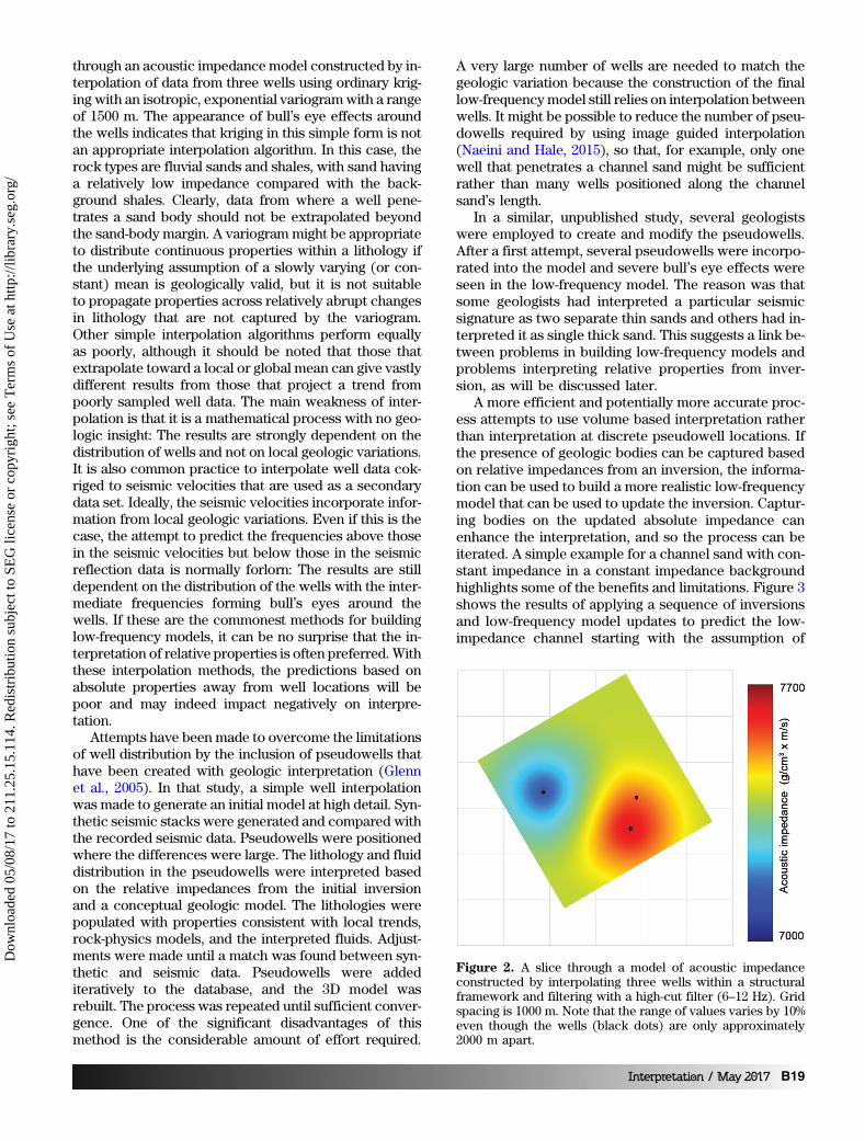
through an acoustic impedance model constructed by in-terpolation of data from three wells using ordinary krig-ing with an isotropic, exponential variogramwith a rangeof 1500 m. The appearance of bull’s eye effects aroundthe wells indicates that kriging in this simple form is notan appropriate interpolation algorithm. In this case, therock types are fluvial sands and shales, with sand havinga relatively low impedance compared with the back-ground shales. Clearly, data from where a well pene-trates a sand body should not be extrapolated beyondthe sand-body margin. A variogram might be appropriateto distribute continuous properties within a lithology ifthe underlying assumption of a slowly varying (or con-stant) mean is geologically valid, but it is not suitableto propagate properties across relatively abrupt changesin lithology that are not captured by the variogram.Other simple interpolation algorithms perform equallyas poorly, although it should be noted that those thatextrapolate toward a local or global mean can give vastlydifferent results from those that project a trend frompoorly sampled well data. The main weakness of inter-polation is that it is a mathematical process with no geo-logic insight: The results are strongly dependent on thedistribution of wells and not on local geologic variations.It is also common practice to interpolate well data cok-riged to seismic velocities that are used as a secondarydata set. Ideally, the seismic velocities incorporate infor-mation from local geologic variations. Even if this is thecase, the attempt to predict the frequencies above thosein the seismic velocities but below those in the seismicreflection data is normally forlorn: The results are stilldependent on the distribution of the wells with the inter-mediate frequencies forming bull’s eyes around thewells. If these are the commonest methods for buildinglow-frequency models, it can be no surprise that the in-terpretation of relative properties is often preferred. Withthese interpolation methods, the predictions based onabsolute properties away from well locations will bepoor and may indeed impact negatively on interpre-tation.

Attempts have been made to overcome the limitationsof well distribution by the inclusion of pseudowells thathave been created with geologic interpretation (Glennet al., 2005). In that study, a simple well interpolationwas made to generate an initial model at high detail. Syn-thetic seismic stacks were generated and compared withthe recorded seismic data. Pseudowells were positionedwhere the differences were large. The lithology and fluiddistribution in the pseudowells were interpreted basedon the relative impedances from the initial inversionand a conceptual geologic model. The lithologies werepopulated with properties consistent with local trends,rock-physics models, and the interpreted fluids. Adjust-ments were made until a match was found between syn-thetic and seismic data. Pseudowells were addediteratively to the database, and the 3D model wasrebuilt. The process was repeated until sufficient conver-gence. One of the significant disadvantages of thismethod is the considerable amount of effort required.

A very large number of wells are needed to match thegeologic variation because the construction of the finallow-frequencymodel still relies on interpolation betweenwells. It might be possible to reduce the number of pseu-dowells required by using image guided interpolation(Naeini and Hale, 2015), so that, for example, only onewell that penetrates a channel sand might be sufficientrather than many wells positioned along the channelsand’s length.

In a similar, unpublished study, several geologistswere employed to create and modify the pseudowells.After a first attempt, several pseudowells were incorpo-rated into the model and severe bull’s eye effects wereseen in the low-frequency model. The reason was thatsome geologists had interpreted a particular seismicsignature as two separate thin sands and others had in-terpreted it as single thick sand. This suggests a link be-tween problems in building low-frequency models andproblems interpreting relative properties from inver-sion, as will be discussed later.

A more efficient and potentially more accurate proc-ess attempts to use volume based interpretation ratherthan interpretation at discrete pseudowell locations. Ifthe presence of geologic bodies can be captured basedon relative impedances from an inversion, the informa-tion can be used to build a more realistic low-frequencymodel that can be used to update the inversion. Captur-ing bodies on the updated absolute impedance canenhance the interpretation, and so the process can beiterated. A simple example for a channel sand with con-stant impedance in a constant impedance backgroundhighlights some of the benefits and limitations. Figure 3shows the results of applying a sequence of inversionsand low-frequency model updates to predict the low-impedance channel starting with the assumption of

Figure 2. A slice through a model of acoustic impedanceconstructed by interpolating three wells within a structuralframework and filtering with a high-cut filter (6–12 Hz). Gridspacing is 1000 m. Note that the range of values varies by 10%even though the wells (black dots) are only approximately2000 m apart.

Interpretation / May 2017 B19

Dow

nloa

ded

05/0

8/17

to 2

11.2

5.15

.114

. Red

istr

ibut

ion

subj

ect t

o SE

G li

cens

e or

cop

yrig

ht; s

ee T

erm

s of

Use

at h

ttp://

libra

ry.s

eg.o

rg/

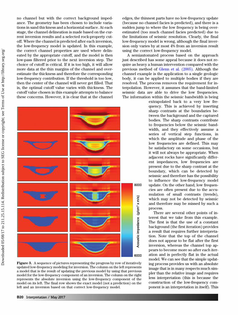
no channel but with the correct background imped-ance. The geometry has been chosen to include varia-tions in sand thickness and a horizontal surface. At eachstage, the channel delineation is made based on the cur-rent inversion results and a selected rock-property cut-off. Where the channel is predicted after each inversion,the low-frequency model is updated. In this example,the correct channel properties are used where delin-eated by the appropriate cutoff, and the model is thenlow-pass filtered prior to the next inversion step. Thechoice of cutoff is critical. If it is too high, it will allowmore data at the thin margins of the channel and over-estimate the thickness and therefore the correspondinglow-frequency contribution. If the threshold is too low,then the center of the channel will never get filled. Thatis, the optimal cutoff value varies with thickness. Thecutoff value chosen in this example attempts to balancethese concerns. However, it is clear that at the channel

edges, the thinnest parts have no low-frequency update(because no channel facies is predicted), and there is asudden jump to where the low frequency is being over-estimated (too much channel facies predicted) due tothe limitations of seismic resolution. Clearly, the finallow-frequency model is wrong, although the final inver-sion only varies by at most 4% from an inversion resultusing the correct low-frequency model.

A semiautomated process based on the approachjust described has some appeal because it does not re-quire as heavy a human intervention compared with theprevious method of Glenn et al. (2005). Although thechannel example is the application to a single geologicbody, it can be applied to multiple bodies if they areresolved. The process removes the requirement for in-terpolation. However, it assumes that the band-limitedseismic data are able to drive the low frequencies.The information within the seismic bandwidth is being

extrapolated back to a very low fre-quency. This is achieved by insertingsharp contrasts at the boundaries be-tween the background and the capturedbodies. The sharp contrasts contributeto frequencies below the seismic band-width, and they effectively assume aseries of vertical step functions, inwhich the amplitude and phase of thelow frequencies are defined. This maybe satisfactory on some occasions, butit will not always be appropriate. Whenadjacent rocks have significantly differ-ent impedances, low frequencies arepresent due to the sharp contrast at theboundary, which can be detected byseismic and therefore has the possibilityto influence the low-frequency modelupdate. On the other hand, low frequen-cies are often present due to the accu-mulation of small contrasts (trends),which may not be detected by seismicand therefore may be missed by such aprocess.

There are several other points of in-terest that we take from this example.The first is that the use of a constantbackground (the first iteration) providesa result that requires further interpreta-tion. Note that the top of the channeldoes not appear to be flat after the firstinversion, whereas the channel top ap-pears to become more so after each iter-ation and is perfectly flat in the actualmodel. We can see that the simple updat-ing process provides us with an absoluteimage that is in many respects much sim-pler than the relative image and requiresless interpretation (this is because theconstruction of the low-frequency com-ponent is an interpretation in itself). This

Figure 3. A sequence of pictures representing the progress by row of iterativelyupdated low-frequency modeling for inversion. The column on the left representsa model that is the result of updating the previous model by using that previousmodel for the low-frequency component of an inversion. The column on the rightrepresents the absolute inversion using the low-frequency component of themodel on its left. The final row shows the exact model (not a prediction) on theleft and an inversion based on that correct low-frequency model.

B20 Interpretation / May 2017

Dow

nloa

ded

05/0

8/17

to 2

11.2

5.15

.114

. Red

istr

ibut

ion

subj

ect t

o SE

G li

cens

e or

cop

yrig

ht; s

ee T

erm

s of

Use

at h

ttp://

libra

ry.s

eg.o

rg/

suggests that despite it being wrong, the final low-fre-quency model is worth pursuing even if only to providea better representation of the body. The final inversion isclearly wrong for the thin edges, and therefore will notprovide accurate quantitative estimates of, say, net sand.The reason is because we either do not capture the bodybecause the cutoff is too harsh, or we capture too muchdue to tuning effects. Note that although inversion im-proves the resolution (accurate quantification of thetop and base of such a body) over seismic reflection data,it can only do this if the low-frequency model is correct.For the thin margins, at the first iteration, the low fre-quency is not correct and the bandwidth has not beenincreased. Because this causes the incorrect estimationof the thickness and therefore the low-frequency model,the resolution either does not improve or gets worse forthe thin margins.

Another point of interest is that when the low-fre-quency model is wrong, for example, after the first in-version with a constant low-frequency model, there arestrong side lobes. Such artifacts can be used to identifypotential errors in low-frequency models. If the inversionis run when the low-impedance channelis populated with too high or too lowimpedances, there are either high-imped-ance sidelobes or low-impedance halos.Although this is easy to see for this sim-ple model, it can be quite hard to judgewhen there are a lot of seismic reflec-tions that interfere and when there isnoise in the data, as is most often thecase for real seismic data. It should alsobe noted that if there were low- and high-impedance events, such as a low-imped-ance channel in the presence of tightsands, that needed to be included inthe low-frequency model, the updatesmust be done carefully. For example,an automatic body capturing interpreta-tion might capture side lobes rather thanactual bodies. That is, the process is notalways simple and additional user inter-action and interpretation might berequired. Processes such as the applica-tion of a threshold combined with con-nectivity criteria and lateral smoothingcan be used.

A real data example of this process istaken from the Gulf of Thailand. Here,the logged strata are Tertiary in ageand typical of many parts of the Gulf ofThailand and portions of other Tertiarysedimentary basins in Southeast Asia. Inthis example, a large portion of the Mio-cene succession several thousand feetthick is comprised of an alternating se-quence of red-bedded sandstone andshale, which forms the target zone forthe seismic inversion. Comparison of

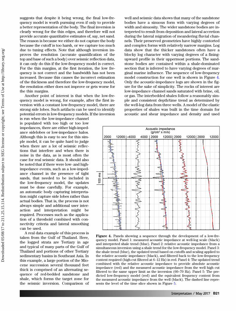
well and seismic data shows that many of the sandstonebodies have a sinuous form with varying degrees ofwidth and sinuosity. The wider sandstone bodies are in-terpreted to result from deposition and lateral accretionduring the lateral migration of meandering fluvial chan-nels. Their preserved geometries have highly contortedand complex forms with relatively narrow margins. Logdata show that the thicker sandstones often have ablocky log character with varying degrees of a fining-upward profile in their uppermost portions. The sand-stone bodies are contained within a shale-dominatedsection that is inferred to have varying degrees of mar-ginal marine influence. The sequence of low-frequencymodel construction for one well is shown in Figure 4.Only the acoustic-impedance logs are shown in the fig-ure for the sake of simplicity. The rocks of interest arelow-impedance channel sands saturated with brine, oil,or gas. The interbedded shales follow a reasonably sim-ple and consistent depth/time trend as determined bythe well-log data from three wells. A model of the elasticproperties of shales was built in the time domain foracoustic and shear impedance and density and used

Figure 4. Panels showing a sequence through the development of a low-fre-quency model. Panel 1: measured acoustic impedance at well-log scale (black)and interpreted shale trend (blue). Panel 2: relative acoustic impedance from asimultaneous inversion using a shale trend for the low-frequency model. Panel 3:the shale trend (blue), the updated trend based on cutoffs and scaling applied tothe relative acoustic impedance (black), and filtered back to the low-frequencycontent required (high-cut filtered at 6–12 Hz) in red. Panel 4: The updated trendcombined with the relative acoustic impedance to provide absolute acousticimpedance (red) and the measured acoustic impedance from the well high cutfiltered to the same upper limit as the inversion (60–70 Hz). Panel 5: The pre-dicted low-frequency model (red) and the equivalent frequency content fromthe measured acoustic impedance from the well (black). The dashed line repre-sents the level of the time slice shown in Figure 5.

Interpretation / May 2017 B21

Dow

nloa

ded

05/0

8/17

to 2

11.2

5.15

.114

. Red

istr

ibut

ion

subj

ect t

o SE

G li

cens

e or

cop

yrig

ht; s

ee T

erm

s of

Use

at h

ttp://

libra

ry.s

eg.o

rg/

as a low-frequency model in a simultaneous inversion.The seismic angle stack data (five stacks ranging from5° to 40°) used in the inversion were low-cut filtered (6–12 Hz linear filter) to avoid any possibility for the seis-mic reflection data to directly contribute to the lowfrequencies in the final model. A standard simultaneousinversion was run using the shale trends as a low-fre-quency model to produce the absolute elastic properties.The relative elastic properties were calculated throughthe application of a band-pass filter and for acousticimpedance produced a high correlation (>0.8) with thewell data within the equivalent bandwidth. The next stepwas to update the initial shale-based low-frequencymodel. First, the distribution of sand and shale was de-termined by applying cutoffs to the relative elastic prop-erty results. The shale trends were then modified wheresands were interpreted to be. There are different possibil-ities for populating these interpreted sands with elasticproperties. One possibility is to use depth trends derivedfrom the well data. This would ideally include differenttrends for different fluids, which would require delinea-tion of fluids from the first-pass inversion. Another ap-proach, which was used for this study, is to set therelative elastic properties to zero within the interpretedshales prior to adding these modified relative propertiesto the shale trends. The sharp changes in the modifiedrelative properties at the upper and lower boundariesof the interpreted sands will then contribute to the lowfrequencies. This approach avoids the need to interpretthe fluid content of the sands prior to the next iterationof inversion. It was found to be necessary to apply aglobal scaling to the modified relative elastic propertiesprior to adding to the shale trend. The scaling was ad-justed to optimize the match of the predicted low fre-quency of the model to the low-frequency componentof the well-log data. This updated low-frequency modelwas then used for a new inversion.

The prediction of the low-frequency componentshown in the final panel of Figure 4 is very good. A com-

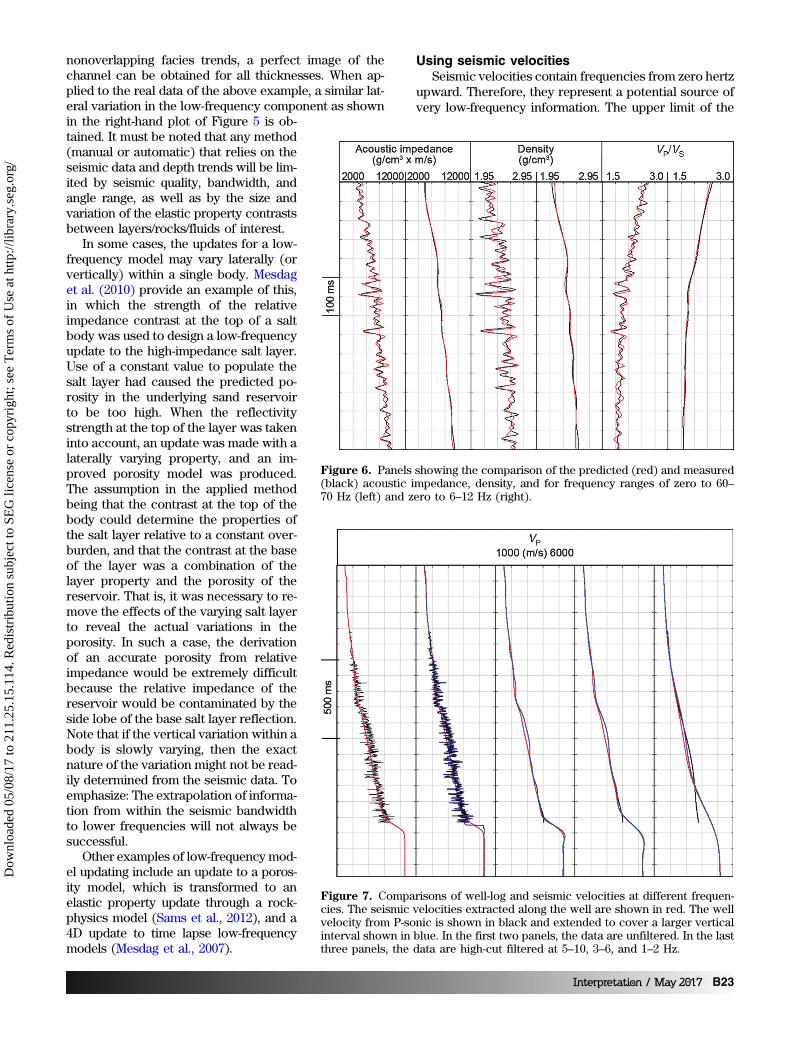
parison is made between the measured well-log acous-tic impedance and the predicted acoustic impedancewith a band-pass filter with corner points of 1–2–6–12 Hz applied. The lowest frequencies were removedbecause those data come predominantly from the basicshale trend and not the update. The correlation of thisband-pass filtered prediction with the equivalent band-pass filtered well-log data is 0.94 with an rms error of60 g∕cm3 ×m∕s. By comparison, if the low-frequencymodel is constructed based on the extrapolation of thefirst well drilled, then the equivalent correlation at thiswell is only 0.75 with an rms error of 288 g∕cm3 ×m∕s.Even when the three wells are considered together, aninterpolation does not honor the variations within thelow-frequency model caused by the complex distribu-tion of the channels in time and space. Figure 5 com-pares a time slice through the acoustic impedance low-frequency models derived from interpolation of thethree wells (left) and through the updated shale trendmodel (right). The differences are obvious. It should benoted that simple interpolation provides accurate re-sults at the wells, but the updating method is not per-fect. The updating process will never be perfect for avariety of reasons that include seismic data quality andresolution limits, but the errors in this case are smallcompared with the errors from simple interpolationaway from well control. The low-frequency models forshear impedance and density have been updated in asimilar fashion (Figure 6). The good correlation for den-sity suggests that it is being accurately predicted fromthe inversion and low-frequency model update. There isno implication, however, that density can be predicteddirectly from reflection data through simultaneous in-version. The simultaneous inversion algorithm usedhere includes a constraint between acoustic impedanceand density, which is dominating the density solutionfor the settings chosen. Note that if the relative proper-ties from the first-pass inversion are not correct, the er-rors will impact the low-frequency model update, and

therefore the errors in the relative inver-sion and low-frequency model will becompounded in the absolute properties.

A full automation of this process canbe achieved (Kemper and Gunning,2014), in which the simultaneous inver-sion solves for the distribution of faciesand elastic properties. The low-frequencymodel is a product of the inversion, and itis constrained by the elastic propertydepth trends associated with each faciesand the inverted distribution of the fa-cies. This fully automated process hasthe potential to improve on the manuallyupdated process in particular with regardto very thin beds because the limits ofresolution can be overcome when condi-tions are favorable. When applied to thesimple channel case shown earlier (Fig-ure 3) with noise-free seismic data and

Figure 5. The left map shows a time slice through an acoustic impedance low-frequency model constructed by interpolation of three wells. The map on theright shows the same slice through a low-frequency model constructed throughan update of a shale trend using the relative impedance results from a first-passinversion. It is shown in Appendix A that it would require a well spacing of ap-proximately 150 m to achieve an appropriate result through well interpolation.

B22 Interpretation / May 2017

Dow

nloa

ded

05/0

8/17

to 2

11.2

5.15

.114

. Red

istr

ibut

ion

subj

ect t

o SE

G li

cens

e or

cop

yrig

ht; s

ee T

erm

s of

Use

at h

ttp://

libra

ry.s

eg.o

rg/

nonoverlapping facies trends, a perfect image of thechannel can be obtained for all thicknesses. When ap-plied to the real data of the above example, a similar lat-eral variation in the low-frequency component as shownin the right-hand plot of Figure 5 is ob-tained. It must be noted that any method(manual or automatic) that relies on theseismic data and depth trends will be lim-ited by seismic quality, bandwidth, andangle range, as well as by the size andvariation of the elastic property contrastsbetween layers/rocks/fluids of interest.

In some cases, the updates for a low-frequency model may vary laterally (orvertically) within a single body. Mesdaget al. (2010) provide an example of this,in which the strength of the relativeimpedance contrast at the top of a saltbody was used to design a low-frequencyupdate to the high-impedance salt layer.Use of a constant value to populate thesalt layer had caused the predicted po-rosity in the underlying sand reservoirto be too high. When the reflectivitystrength at the top of the layer was takeninto account, an update was made with alaterally varying property, and an im-proved porosity model was produced.The assumption in the applied methodbeing that the contrast at the top of thebody could determine the properties ofthe salt layer relative to a constant over-burden, and that the contrast at the baseof the layer was a combination of thelayer property and the porosity of thereservoir. That is, it was necessary to re-move the effects of the varying salt layerto reveal the actual variations in theporosity. In such a case, the derivationof an accurate porosity from relativeimpedance would be extremely difficultbecause the relative impedance of thereservoir would be contaminated by theside lobe of the base salt layer reflection.Note that if the vertical variation within abody is slowly varying, then the exactnature of the variation might not be read-ily determined from the seismic data. Toemphasize: The extrapolation of informa-tion from within the seismic bandwidthto lower frequencies will not always besuccessful.

Other examples of low-frequency mod-el updating include an update to a poros-ity model, which is transformed to anelastic property update through a rock-physics model (Sams et al., 2012), and a4D update to time lapse low-frequencymodels (Mesdag et al., 2007).

Using seismic velocitiesSeismic velocities contain frequencies from zero hertz

upward. Therefore, they represent a potential source ofvery low-frequency information. The upper limit of the

Figure 6. Panels showing the comparison of the predicted (red) and measured(black) acoustic impedance, density, and for frequency ranges of zero to 60–70 Hz (left) and zero to 6–12 Hz (right).

Figure 7. Comparisons of well-log and seismic velocities at different frequen-cies. The seismic velocities extracted along the well are shown in red. The wellvelocity from P-sonic is shown in black and extended to cover a larger verticalinterval shown in blue. In the first two panels, the data are unfiltered. In the lastthree panels, the data are high-cut filtered at 5–10, 3–6, and 1–2 Hz.

Interpretation / May 2017 B23

Dow

nloa

ded

05/0

8/17

to 2

11.2

5.15

.114

. Red

istr

ibut

ion

subj

ect t

o SE

G li

cens

e or

cop

yrig

ht; s

ee T

erm

s of

Use

at h

ttp://

libra

ry.s

eg.o

rg/

frequency content depends on how the velocities werepicked or generated. In some cases in which automatichigh-density velocity analysis or full-waveform inversionhas been performed, the frequency content can be quitehigh, perhaps 4 or 5 Hz. However, this should not be con-fused with the upper limit of useful frequency content.Extraction of the seismic velocity along well tracksand comparison with good quality sonic logs or check-shot velocities often indicates that the upper frequencylimit of reliable information for use in constructing low-frequency models for inversion is no higher than 2 Hzand sometimes much less. Even then, there are usuallysystematic variations between well-log velocities andseismic velocities, for example, as discussed in Appen-dix B. It is common, therefore, to condition the seismicvelocities through vertical and lateral filtering and toapply a calibration process to reconcile the seismicvelocities to the well velocities. Several problems are en-countered during this conditioning and calibration. First,how to choose the optimal frequency filter to apply;

second, how to accurately calculate calibration factorswhen the well data are usually of limited extent, andtherefore have high uncertainty in the very low-fre-quency (0–2 Hz) content; third, whether there is a goodreason for calibration or whether the data are of insuffi-cient quality; and fourth, how to interpolate calibrationfactors between wells.

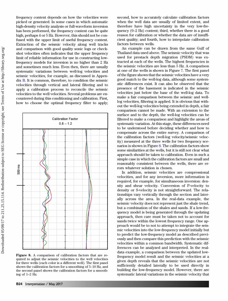
An example can be drawn from the same Gulf ofThailand data used above. The seismic velocity that wasused for prestack depth migration (PSDM) was ex-tracted at each of the wells. The highest frequencies inthe seismic velocities are less than 5 Hz. A comparisonat one of the wells is shown in Figure 7. The first panelof the figure shows that the seismic velocities have a verygood match to the well-log data, although some system-atic differences exist. It can also be observed that thepresence of the basement is indicated in the seismicvelocities just below the base of the well-log data. Tomake a fair comparison between the seismic and well-log velocities, filtering is applied. It is obvious that with-out the well-log velocities being extended in depth, a faircomparison cannot be made. With an extension to thesurface and to the depth, the well-log velocities can befiltered to make a comparison and highlight the areas ofsystematic variation. At this stage, these differences needto be understood before deciding whether and how tocompensate across the entire survey. A comparison ofthe calibration factors (well-log velocity/seismic veloc-ity) measured at the three wells for two frequency sce-narios is shown in Figure 8. The calibration factors showsome similarities at the wells, but it is still not clear whatapproach should be taken to calibration. Even in such asimple case in which the calibration factors are small andreasonably consistent between the wells, there are er-rors whatever solution is chosen.

In addition, seismic velocities are compressionalvelocities, and for any inversion, more information isrequired, for example, for simultaneous inversion: den-sity and shear velocity. Conversion of P-velocity todensity or S-velocity is not straightforward. The rela-tionships vary vertically through the section and later-ally across the area. In the real-data example, theseismic velocity does not represent just the shale trend,but a combination of the shales and sands. If a low-fre-quency model is being generated through the updatingapproach, then care must be taken not to account forsands twice within the lowest frequency range. One ap-proach would be to not to attempt to integrate the seis-mic velocities into the low-frequency model initially butto predict the low-frequency model as described previ-ously and then compare this prediction with the seismicvelocities within a common bandwidth. Systematic dif-ferences can be analyzed and interpreted. In the real-data example, a comparison between the updated low-frequency model result and the seismic velocities at agiven depth reveals that the seismic velocities are notsufficiently detailed laterally to be used directly inbuilding the low-frequency model. However, there aresystematic lateral variations in the seismic velocity that

Figure 8. A comparison of calibration factors that are re-quired to adjust the seismic velocities to the well velocitiesfor three wells (each color is a different well). The first panelshows the calibration factors for a smoothing of 5–10 Hz, andthe second panel shows the calibration factors for a smooth-ing of 1–2 Hz.

B24 Interpretation / May 2017

Dow

nloa

ded

05/0

8/17

to 2

11.2

5.15

.114

. Red

istr

ibut

ion

subj

ect t

o SE

G li

cens

e or

cop

yrig

ht; s

ee T

erm

s of

Use

at h

ttp://

libra

ry.s

eg.o

rg/

might need to be incorporated in the low-frequencymodel (Figure 9). There is evidence that the variationsin the seismic velocities correlate to the depth of thebasement and that the current assumption of a flat da-tum for shale trends in the inversion is insufficient awayfrom the well control. Therefore, an approach herewould be to use the lateral variations in the seismicvelocities to establish a variable shale trend for useas a starting model for the inversion and then update.

ConclusionIn a deterministic framework, uncertainties are

ignored and choices are made to produce the most likelyresult given the current data and information. For seis-mic inversion, choices are made that affect the relativeand the absolute elastic properties. The examples shownin this paper strongly suggest that the most likely low-fre-quency model cannot be produced prior to an inversionhaving been performed. The simple interpolation of well-log data, even though it may be within a geologic frame-work and somehow conditioned to seismic velocities,will usually produce a low-frequency model that is mean-ingfully different from the most likely. Unfortunately,there is strong evidence, as provided by many publica-tions and presentations, that in practice most low-fre-quency models are constructed prior to inversion andnot revisited before interpretation of the absolute elasticproperties. Under such circumstances, it is often betterto only interpret the relative impedances. Indeed, manyproject objectives might be achieved to a sufficient de-gree through relative impedance interpretation. On theother hand, interpretation of relative impedances is notnecessarily straightforward. The major issue being thatrelative impedances are only relative and can be misin-terpreted without constructing either explicitly or withinthe interpreter’s mind a possible low-frequency model.The example cited in the Introduction of normally pres-sured sands in an environment, in which the boundingshales are variously pressured, is best explored in theabsolute domain, in which a low-frequency model hasbeen developed that possibly includes information from

the seismic velocities, assuming that theyare of sufficient quality.

The methods for improving theconstruction of low-frequency models,outlined in this paper, imply that low-frequency model construction is an in-terpretation and prediction process thatattempts to produce broad bandwidthabsolute impedance models that areconsistent with the relative impedances,well data, and seismic velocities as wellas any rock physics and geologic con-straints that are known. The aim is toproduce the most likely result for allfrequencies from zero up to the highestfrequencies in the seismic data without

constraining any particular frequency range to strictlyhonor the well data. The methods rely in part on ex-trapolating information from within the seismic band-width to lower frequencies. This process will not alwaysbe appropriate; for example, errors in the manual or au-tomatic interpretation of relative impedances wouldcause the low-frequency model to be wrong. If a singlethick body is misinterpreted as two separate bodiesfrom relative impedance, this error might never be cor-rected through an iterative update of the low-frequencymodel. What is important is that there should be a shiftin focus from concern about if and how a low-frequencymodel is biasing the interpretation of an inversion resultto a concern about how to interpret relative imped-ances from an inversion, in the absence of low frequen-cies. Building a low-frequency model as part of theinversion process is one method of interpreting relativeimpedances and takes us one step further from seismicreflection data and closer to an accurate model ofthe rocks.

AcknowledgmentsThe authors would like to thank Kris Energy and

partners, Mubadala Petroleum, and Northern Gulf forpermission to present their data.

Appendix A

Problems with well data interpolationLaterally, fluvial sandstone bodies often show clearly

defined margins by lateral discontinuities of seismicamplitude or impedance, which result from their depo-sition in association within a relatively narrow fluvialchannel. In many cases, a fluvial sandstone body is theresult of sandbar formation and lateral accretion duringits deposition, which in turn results in variations in thepreserved sandstone body width and thickness. Thesecharacteristics are typical of many fluvial reservoirsthat are exploited for oil and gas worldwide. In termsof 3D seismic data, a sandstone body’s laterally con-fined margin often approaches a step function of imped-ance in horizontal (XY) space (on the scale of theseismic resolution); all spatial frequencies are needed

Figure 9. A slice through the predicted acoustic impedance high-cut filtered at1–2 Hz (left) and the seismic velocity high-cut filtered at 1–2 Hz (right). A con-stant density is used to transform the color bar of acoustic impedance to velocity,so that the scales are comparable.

Interpretation / May 2017 B25

Dow

nloa

ded

05/0

8/17

to 2

11.2

5.15

.114

. Red

istr

ibut

ion

subj

ect t

o SE

G li

cens

e or

cop

yrig

ht; s

ee T

erm

s of

Use

at h

ttp://

libra

ry.s

eg.o

rg/

to describe a lateral step function accurately. Samplingtheorem dictates that the lateral sample spacing of regu-lar sampled data must be less than or equal to a halfcycle of a spatial frequency component for it to be rep-resented correctly. In a 3D seismic data set, the highestspatial frequency of the temporal signal present is lim-ited by its associated first Fresnel zone width, to varyingdegrees by structural dip, or by the seismic acquisitiongeometry and process, for example, the bin size that de-fines the spatial Nyquist frequency of the seismic data.In contrast, low spatial frequencies are generally over-sampled.

If a low-frequency model for seismic amplitude inver-sion is derived by an interpolation of well data alone,then the local well spacing itself defines a spatial Ny-quist frequency for the interpolated low-frequency com-ponents. As such, the local average well spacing mustbe less than or equal to a half-cycle of the maximumspatial frequency component being interpolated for itto be represented appropriately; the azimuthal distribu-tion of wells are also an important contributing factor.

In traditional inversion methods, the seismic tempo-ral frequency bandwidth often dictates the choice ofan upper frequency limit in a well-based low-frequencymodel, for example, the lowest effective signal fre-quency component present in the seismic data. Thischoice in turn limits the minimum lateral sample spac-ing necessary to interpolate the low-frequency modelspatially to an equivalent degree as the seismic data. Forexample, the typical lowest effective temporal frequencyin a seismic data set might be approximately 10 Hz(although this is being reduced via improved seismic ac-quisition methods in some areas). The Fresnel zone of a10 Hz temporal frequency component collapses to a150 m diameter, assuming a velocity of 3000 m∕s andperfect 3D migration; the process ideally collapsing theFresnel zone diameter to a half wavelength of the asso-ciated temporal frequency (Bacon et al., 2003). Clearly,in this 10 Hz example, a well spacing of 150 m that mayprovide adequate sampling is rarely achieved in oil andgas fields. Such laterally undersampled well data oftenlead to aliasing in the spatial frequency domain thatcauses bull’s eye effects in traditional low-frequencymodels and their associated seismic amplitude inversionresults. In laterally undersampled situations, a particularspatial frequency component being interpolated, butundersampled, doubles back around the spatial Nyquistfrequency, and it is represented by an artificially lowerspatial frequency component (given that lateral well dis-tribution). This is the principal physical reason why thesimple spatial interpolation of well data is often inappro-priate.

In the oil and gas fields of the Gulf of Thailand, fromwhere the main example in the paper originates, wellspacing varies dramatically on the scale of several hun-dred meters to several kilometers. Here, the averagewell spacing may be as low as 400 m (Harr et al., 2011),although this is often along a locally preferred azimuth,for example, being parallel to a nearby fault. In this lat-

ter situation, spatial aliasing of a 10 Hz frequency bandmay still occur during simple well-based data interpola-tion, but the azimuth-dependent spatial Nyquist fre-quency often results in a preferred azimuthal bias inthe distortion caused by the spatial aliasing process(seen to some extent in Figure 5). Clearly, if the tightlaterally sampled seismic data could be used reliably tomap the low-spatial-frequency components, as an alter-native to traditional methods, then the detrimentaleffects of spatial aliasing in a low-frequency modelcould be minimized.

Appendix B

Reliability of seismic velocitiesThe process of seismic velocity estimation incorpo-

rates a large range of factors that may influence thequality and reliability of velocity estimates. Such factorsarise from seismic acquisition and its surface environ-ment, the geologic succession, seismic processing, andvelocity interpretation.

Velocity estimates from prestack time migrated(PSTM) seismic data suffer from the fact that they oftenpreserve a signature from a relatively large area of theoverburden. For example, a lateral step function of in-terval velocity in the overburden results in a lateralwavelet-like distortion in the PSTM velocity estimatesat a target level below (Toldi, 1984). This results fromthe associated raypaths of individual source-receiverpairs that comprise a prestack gather. The lateral di-mension of such a distortion can approach several kilo-meters, and it is a function of (1) the depth differencebetween the target and the lateral velocity change,(2) the velocity gradient, and (3) the acquisition geom-etry, for example, the effective streamer length of amarine seismic survey. In reality, many such lateralvelocity variations often occur in the overburden, par-ticularly in a channel sand geologic succession, and re-sult in a complex composite distortion. In many cases,such distortions are biased by the preferred source-receiver azimuth distribution during seismic acquisition.Therefore, in some cases, this may form an overridingfactor in the reliability of the PSTM velocity estimates.

In contrast, the iterative velocity model buildingprocesses used in PSDM attempts to collapse this typeof lateral wavelet-like distortion and isolate a lateralstep function of interval velocity in the overburdenvelocity model. However, PSDM velocities are still aproduct of seismic imaging, and the velocity model ofreal data is never perfect. Lateral smoothing is alsooften performed that may degrade the velocity esti-mates. It follows that, in addition to data quality, achoice of whether seismic velocities are to be used ina low-frequency model for inversion may depend on thetype of velocities available, their lateral sampling andprocessing, and in some cases the severity of the over-burden velocity variations. Low-frequency seismic ac-quisition and advanced processing methods, such asthose associated with full-waveform inversion, may

B26 Interpretation / May 2017

Dow

nloa

ded

05/0

8/17

to 2

11.2

5.15

.114

. Red

istr

ibut

ion

subj

ect t

o SE

G li

cens

e or

cop

yrig

ht; s

ee T

erm

s of

Use

at h

ttp://

libra

ry.s

eg.o

rg/

help to provide more reliable velocity estimates for low-frequency models.

ReferencesBacon, M., R. Simm, and T. Redshaw, 2003, 3-D seismic

interpretation: Cambridge University Press.Ball, V., J. P. Blangy, C. Schiott, and A. Chaveste, 2014, Rel-

ative rock physics: The Leading Edge, 33, 276–286, doi:10.1190/tle33030276.1.

Ball, V., L. Tenorio, C. Schiott, J. P. Blangy, and M. Thomas,2015, Uncertainty in inverted elastic properties resultingfrom uncertainty in the low-frequency model: The Lead-ing Edge, 34, 1028–1035, doi: 10.1190/tle34091028.1.

Doyen, P., 2007, Seismic reservoir characterization: Anearth modeling perspective: EAGE Publications bv.

Glenn, D., F. Hariyannurgraha, R. Schneider, K Kirschner,S. Walden, S. Smith, E. Berendson, C. Skelt, L. Lisapaly,R. van Eykenhof, and M. Sams, 2005, Enhancing consis-tency between geological modeling and seismic pre-stack amplitude inversion with pseudo-wells: An exam-ple from the Gendalo Field: 30th Annual Conventionand Exhibition, Indonesian Petroleum Association, Pro-ceedings, IPA05–G029.

Harr, M. S., S. Chokasut, C. Bhuripanyo, P. Viriyasittigun,and R. Harun, 2011, Evaluation of factors in horizontalwell recovery in the Pattani Basin in the Gulf of Thai-land: International Petroleum Technology Conference,IPTC, Paper 14981–MS.

Kemper, M., and J. Gunning, 2014, Joint impedance and fa-cies inversion — Seismic inversion redefined: FirstBreak, 32, 89–95.

Latimer, R. B., R. Davison, and P. van Riel, 2000, An inter-preter’s guide to understanding and working with seis-mic-derived acoustic impedance data: The LeadingEdge, 19, 242–256, doi: 10.1190/1.1438580.

Mesdag, P. R., M. Feroci, L. Barens, P. H. Prat, and W.Pillet, 2007, Full bandwidth inversion for time lapsereservoir characterization on the Girassol Field: 69th An-nual International Conference and Exhibition, EAGE,Extended Abstracts, A032.

Mesdag, P. R., D. Marquez, L. de Groot, and V. Aubin, 2010,Updating low frequency model: 72nd Annual Interna-tional Conference and Exhibition, EAGE, Extended Ab-stracts, F027.

Mukerji, T., G. Mavko, and C. Gomez, 2009, Cross-propertyrock physics relations for estimating low-frequencyseismic impedance trends from electromagnetic resis-tivity data: The Leading Edge, 28, 94–97, doi: 10.1190/1.3064153.

Naeini, E. Z., and D. Hale, 2015, Image- and horizon-guidedinterpolation: Geophysics, 80, no. 3, V47–V56, doi: 10.1190/geo2014-0279.1.

Pedersen-Tatalovic, R., A. Uldall, N. L. Jacobsen, T. M.Hansen, and K. Mosegaard, 2008, Event-based low-frequency modeling using well logs and seismic attrib-utes: The Leading Edge, 27, 592–603, doi: 10.1190/1.2919576.

Pendrel, J., and P. van Riel, 2000, Effect of well control onconstrained sparse spike inversion: CSEG Recorder,25, 18–26.

Sams, M. S., T. J. Focht, and J. Ting, 2012, Porosity estima-tion from deterministic inversion: 74th Annual Interna-tional Conference and Exhibition, EAGE, Extended Ab-stracts, X015.

Toldi, J., 1984, Estimation of a near-surface velocity fromstacking velocities: SEP, 41, 99–120.

Biographies and photographs of the authors are notavailable.

Interpretation / May 2017 B27

Dow

nloa

ded

05/0

8/17

to 2

11.2

5.15

.114

. Red

istr

ibut

ion

subj

ect t

o SE

G li

cens

e or

cop

yrig

ht; s

ee T

erm

s of

Use

at h

ttp://

libra

ry.s

eg.o

rg/