1

Large Scale System Modeling:Structuring model libraries

and numerical best practices

Hubertus TummescheitWith material from Luca Bertuccioli and

Lars PedersenUTRC

Outline• Motivation: model & library requirements• Model architecture:

– design patterns for object oriented, equation based modeling• Numerical design patterns

– Non-linear equations, ODE, DAE, PDE– Bounds checking, Scaling – Smoothness– Stiffness

• Best Practices for Equation-based Model Development (version control, testing, …)– Documentation – Naming conventions– Testing

2

Model and model library requirements

• Robust, versatile models for system design– Easy to initialize, fast execution, failures give meaningful errors– Tested in all corners of validity range (testable models)– Models adaptable to simulation and sizing optimization– Documentation

• easy to read and understand models • complete reference & description exists• naming conventions “self-documenting models”).

– Fully documented range of validity• Range of permissible operation is parameter, e.g. 25% – 105%

nominal power – If more than 1 model needed per component to fulfill all the

requirements, these models must be exchangeable (e.g. same degrees of freedom for simulation)

– Clear definition of what information the model needs to provide in design/sizing, off-design or dynamic operation

Homework reading

Library requirements for numerics and connectivity

• Full understanding of all numerical issues– Avoid causing change of mathematical model structure by

connection– Non-linear equation systems: occurrence, complexity, scaling

(usually not an issue in good Modelica libraries)– Hybrid issues: smoothness, unavoidable discontinuities,

connectivity issues, chattering

• Ability to include existing legacy models– Using FORTRAN or C-code, dll’s for part of the model

– Existing legacy code reuse (property functions, terrain)– Handle problems outside of the range of the modeling platform

• Fully modular: no restrictions on model connectivity– Subsystems models have same interfaces & connectivity &

parameters independent of level of detail

Homework reading

3

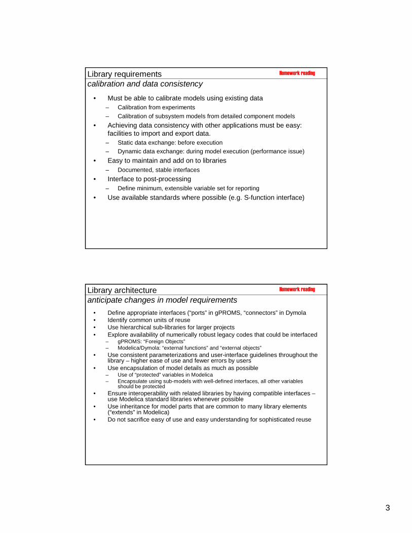
Library requirementscalibration and data consistency

• Must be able to calibrate models using existing data– Calibration from experiments

– Calibration of subsystem models from detailed component models

• Achieving data consistency with other applications must be easy:facilities to import and export data.

– Static data exchange: before execution– Dynamic data exchange: during model execution (performance issue)

• Easy to maintain and add on to libraries– Documented, stable interfaces

• Interface to post-processing– Define minimum, extensible variable set for reporting

• Use available standards where possible (e.g. S-function interface)

Homework reading

Library architectureanticipate changes in model requirements

• Define appropriate interfaces (“ports” in gPROMS, “connectors” in Dymola• Identify common units of reuse• Use hierarchical sub-libraries for larger projects• Explore availability of numerically robust legacy codes that could be interfaced

– gPROMS: “Foreign Objects”– Modelica/Dymola: “external functions” and “external objects”

• Use consistent parameterizations and user-interface guidelines throughout the library – higher ease of use and fewer errors by users

• Use encapsulation of model details as much as possible– Use of “protected” variables in Modelica– Encapsulate using sub-models with well-defined interfaces, all other variables

should be protected • Ensure interoperability with related libraries by having compatible interfaces –

use Modelica standard libraries whenever possible• Use inheritance for model parts that are common to many library elements

(“extends” in Modelica)• Do not sacrifice easy of use and easy understanding for sophisticated reuse

Homework reading

4

Model architecturedesign interfaces and sub-models for modularity and reuse

• Design principle: write models that are easy to use by non-experts! • Structure of each model needs to be consistent with library structure• Consistent parameterizations for all related models• If possible, base on parent class with common interfaces/UI-design

(Modelica)• Document all assumptions and range of validity/applicability• Define and document allowable degrees of freedom (steady-state

models) and boundary & initial conditions (PDE, dynamic models)• Interaction with other models only via defined, visible interfaces (no

“hidden” control-like actions within models) • Encapsulate functional entities that are used by many components

and that might be changed to improve reuse: property calculations for fluids, coordinate transformations in mechanical systems that depend on the parameterization of the orientation.

• Every model needs to have one or more associated test-cases that– Demonstrate robustness of the model in the whole operating range– Provides a simple verification example

Homework reading

Why Design Patterns?

• Recurring problems• Canned solutions• Easy to communicate

• 80 - 90 % of support requests in dynamic modeling answered by a numerical design pattern

5

Why Design Patterns?

• Some design patterns are trivial– but often missed

• Using an object-oriented language is no silver bullet to obtain code reuse.

• Coding style is an important element

Object-Oriented Modeling is notObject-Oriented Programming .

• Static inheritance code structure similar• static data structures very similar• almost identical notation

• run time behavior very different• run time data structures different• different semantics

6

Semantics of OOM and OOP

• Object-oriented Modeling– differential algebraic equations

– discrete time events– difference equations– equations from connecting subsytems– structure at run-time is static

result is one large, hybrid DAEthe complete behavior is used all the time

Semantics of OOM and OOP

• Object-oriented Programming– message passing between objects– methods operate on encapsulated data– objects created and destroyed– dynamic run-time structure

Many executions of a program work if errors are in rarely used methods

Homework reading

7

Encapsulation

• No encapsulation of operations in OOM!• data access can be restricted • parameters can be encapsulated

EncapsulationExample of bad encapsulation properties in OOM:Network of incompressible flows. 2 Types of boundary conditions:• pressure given• flow rate given

p

p

1 unphysical boundary condition and the problem is no longer well-posed

With 3 given mass-flows, the pressure in the system is undefined

8

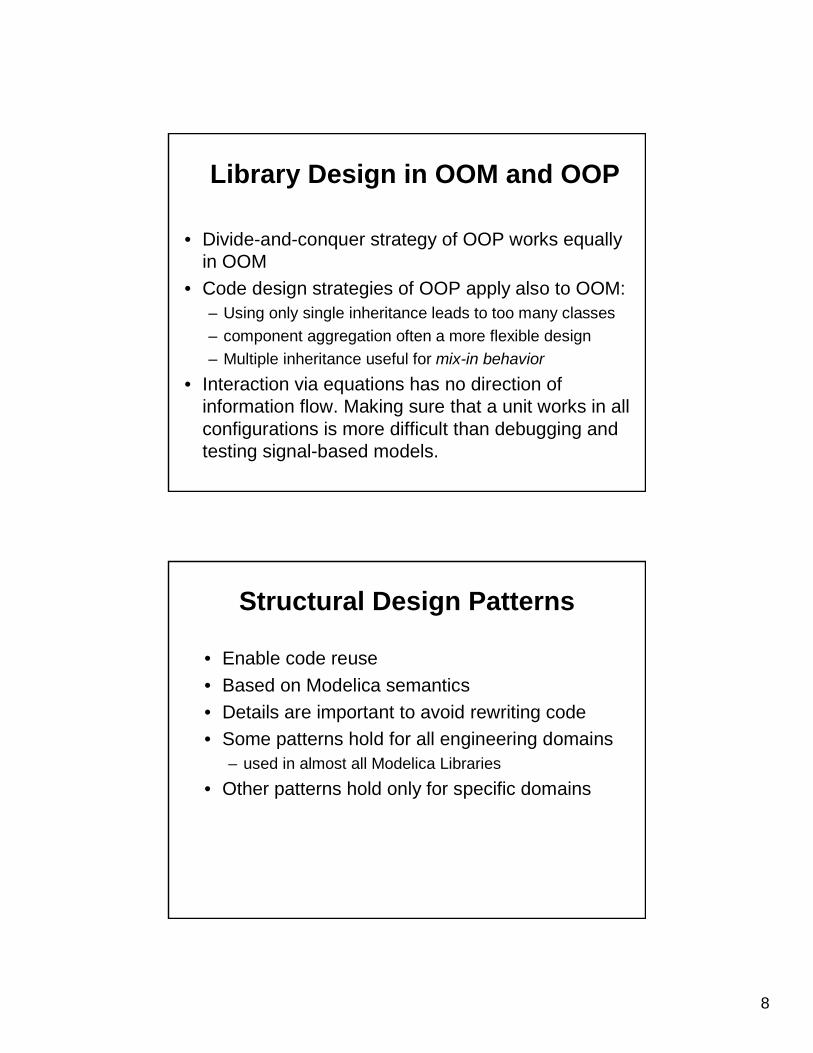
Library Design in OOM and OOP

• Divide-and-conquer strategy of OOP works equally in OOM

• Code design strategies of OOP apply also to OOM:– Using only single inheritance leads to too many classes– component aggregation often a more flexible design – Multiple inheritance useful for mix-in behavior

• Interaction via equations has no direction of information flow. Making sure that a unit works in all configurations is more difficult than debugging and testing signal-based models.

Structural Design Patterns

• Enable code reuse

• Based on Modelica semantics• Details are important to avoid rewriting code• Some patterns hold for all engineering domains

– used in almost all Modelica Libraries

• Other patterns hold only for specific domains

9

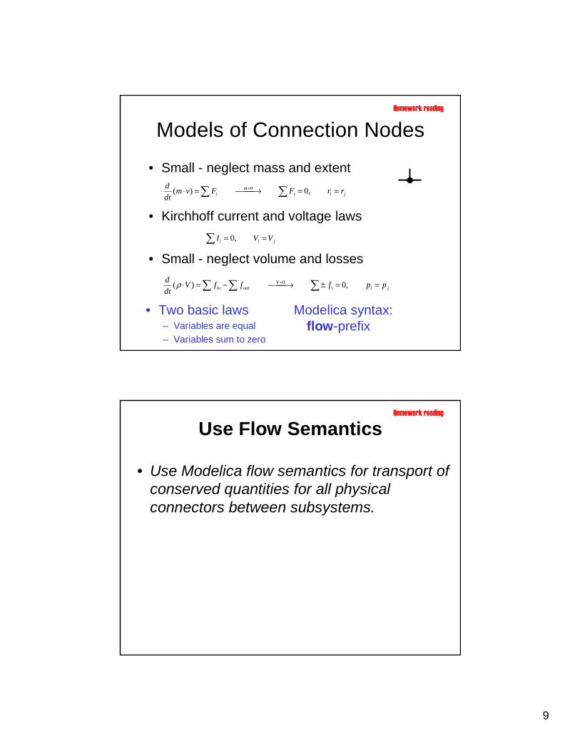
Models of Connection Nodes

• Small - neglect mass and extent

jiim

i rrFFvmdt

d ==→=⋅ ∑∑ = ,0)( 0

• Kirchhoff current and voltage laws

jii VVI ==∑ ,0

• Small - neglect volume and losses

jiiV

outin ppfffVdt

d ==±→−=⋅ ∑∑∑ = ,0)( 0ρ

• Two basic laws– Variables are equal– Variables sum to zero

Modelica syntax:flow-prefix

Homework reading

Use Flow Semantics

• Use Modelica flow semantics for transport of conserved quantities for all physical connectors between subsystems.

Homework reading

10

Use Flow Semantics

• Some engineering domains use it traditionally (Electrical, Mechanical), others not

• Natural for bi-directional interaction• Often omitted for convection models

– the simplest model for flow splitters and junctions in ThermoFluid makes use of flow semantics

Pipe

Homework reading

Connectors Sets

• Provide models with typical configurations in base classes. Implement the physics inside them in derived classes.

p n

p.i n.i

flange_a flange_b

flange axisflange axis

Electrical Library

Translational 1D Mechanics Library

ThermoFluid Library

11

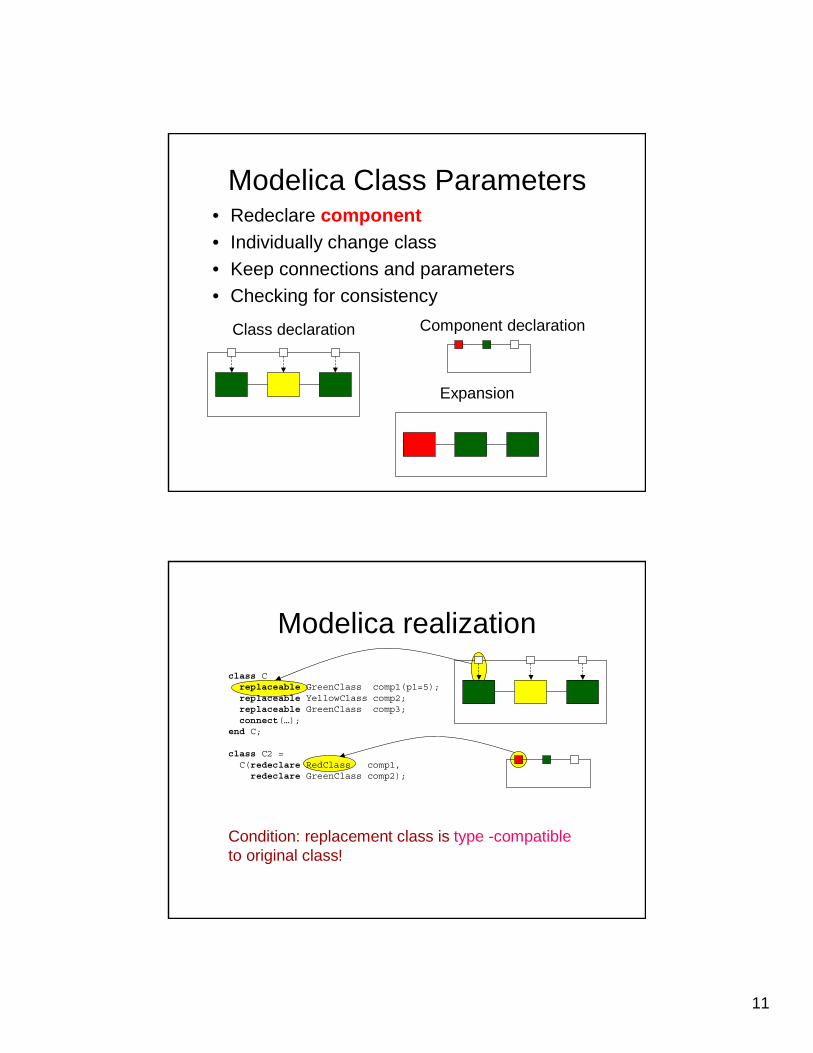
Modelica Class Parameters• Redeclare component• Individually change class• Keep connections and parameters• Checking for consistency

Class declaration Component declaration

Expansion

Modelica realization

class Creplaceable GreenClass comp1(p1=5);replaceable YellowClass comp2;replaceable GreenClass comp3;connect(…);

end C;

class C2 =C(redeclare RedClass comp1,redeclare GreenClass comp2);

Condition: replacement class is type -compatibleto original class!

12

Modelica realization

class CRedClass comp1(p1=5);GreenClass comp2;GreenClass comp3;connect(…);

end C;

Equivalent to

class Creplaceable GreenClass comp1(p1=5);replaceable YellowClass comp2;replaceable GreenClass comp3;connect(…);

end C;

class C2 =C(redeclare RedClass comp1,redeclare GreenClass comp2);

Records for type-compatibility

• Type-compatible: at least the same components, may have extra ones

• May be arbitrary hierarchical structure

• Collect all components that define a replaceable type in a record. Let all models inherit from that record.

13

Records for type-compatibility

• Used in ThermoFluid for fluid properties. Same class with other properties used for Water, CO2 and R134a.

Mathematical Structure and Model Robustness

• Equation types– Non-linear steady-state, ODE, index-1 DAE, High

index DAE, PDE,

• Robustness issues non-linear equations– Scaling (also for ODE, DAE)– Bounds checking– Coordinate transformations – Infinite derivatives– Smoothness

• High-index DAE• Discretization for PDE• Hybrid discrete-continuous models

14

Equation types

• Equation types (often combined)– Non-linear steady-state

• Can be very difficult to solve• Non-convexity of equations & multiple solutions

are common pitfalls

– Mixed continuous-discrete• Even more difficult to solve• Avoid if caused by piecewise discontinuous

correlations that should be continuous on physical reasoning

Equation types

• Equation types (continued)– ODE, index-1 DAE

• Scaling of time, stiffness, choice of frequency range of “interesting dynamics”

– High index DAE• Depending on capabilities of environment,

circumvent (gPROMS) or utilize (Dymola) with proper coding rules (all code needs to be symbolically differentiable!)

– PDE• Choice of time & length scales of interest,

spatial resolution & frequency range matter

15

Solver types and implications for coding guidelines

Write equations that play nicely with all solver types that might be applied to model!

• Newton-based– Smooth, bounded gradients needed (0 and inf are

both bad)

• Combined continuous-discrete methods– Remove non-physical discontinuities– Make unavoidable discontinuities visible to solver,

this may be problematic with discontinuities in external code

Solver types and implications for coding guidelines

• Bounds checking for equation solving– Often needed due to limited ranges of validity and polynomial

approximations– Too tight bounds can cause failure– Too loose bounds may result in final solutions outside the

permissible range.

• Optimization– Smooth, convex problems are much easier to solve than others

models are often adapted to optimization needs– Often necessary to allow loose bounds and check validity for result

as post-condition • Real-time adapted solvers

– Fixed step time for guaranteed max. computation time– Available in Matlab and Dymola, not gPROMS– Errors have to be checked against off-line reference trajectories

Homework reading

16

Scaling of equations / variables

• Ideally try to scale variables so that typical magnitude is 1• Not always practical to do this

• In gPROMS, easier to scale equations• Given the original equation: LHS = RHS• Introduce a scaling factor fscale that is a parameter in your

model• Rewrite equation as: LHS / fscale = RHS / fscale, such that the

new terms on either side of the equation are approximately 1

• In Dymola/Modelica use nominal attribute• E.g. SIunits.Pressure p(nominal = 1.0e5)

Homework reading

Scaling of equations / variables

• Always try to scale your mass, energy and momentum equations

• Don’t hard-code a scaling factor, rather introduce a parameter

• A different value for the factor may be needed depending on the model application (e.g. test-tube or full-size plant)

• Either method (variable scaling or equation scaling) can be used, depending on modeling tool.

Homework reading

17

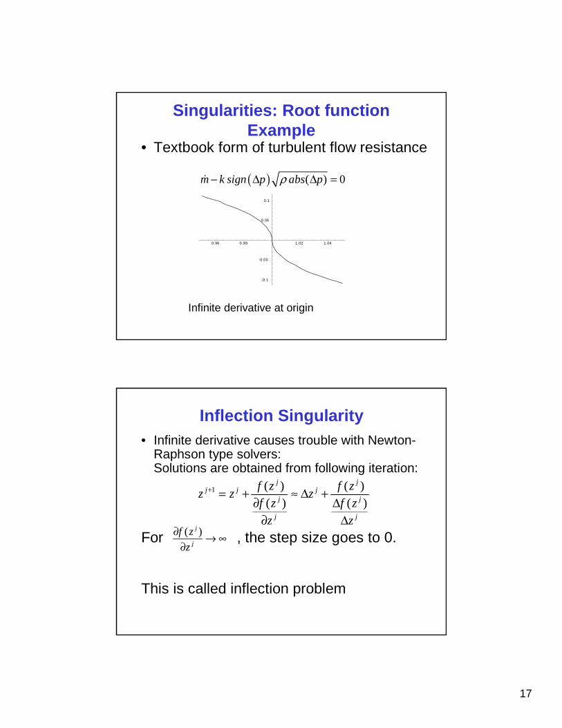
Singularities: Root function Example

( ) ( ) 0m k sign p abs pρ− ∆ ∆ =&

• Textbook form of turbulent flow resistance

0.96 0.98 1.02 1.04

-0.1

-0.05

0.05

0.1

Infinite derivative at origin

Inflection Singularity• Infinite derivative causes trouble with Newton-

Raphson type solvers:Solutions are obtained from following iteration:

For , the step size goes to 0.

This is called inflection problem

1 ( ) ( )( ) ( )

j jj j j

j j

j j

f z f zz z z

f z f z

z z

+ = + ≈ ∆ +∂ ∆

∂ ∆( )j

j

f z

z

∂ → ∞∂

18

Root function remedy

0.96 0.98 1.02 1.04

-0.1

-0.05

0.05

0.1

• Replace singular part with non-singular substitute– result should be qualitatively correct

(quantitative values often unknown)– the function should be C1 continuous

0.96 0.98 1.02 1.04

-0.1

-0.05

0.05

0.1

Root function remedy: How-To

0.96 0.98 1.02 1.04

-0.1

-0.05

0.05

0.1

• Define region where original correlation is replaced by approximation, e.g. 0.01*mdot0

• Simplify the function at that point inserting the limit • Take the symbolic derivative of the function at that

point• Compute polynomial coefficients to match both

function and derivative at connection point 4 equations for 4 unknowns

• The matching point may be a parameter

Homework reading

19

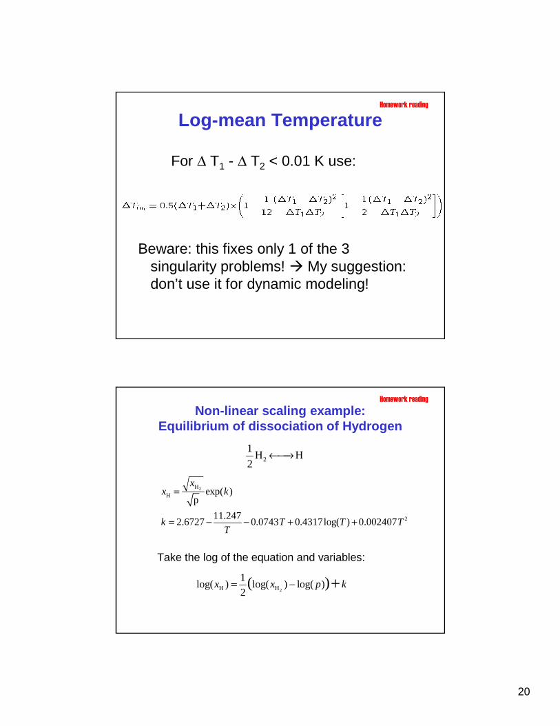
Log-mean Temperature

Log-mean Temperature 1 2

1 2ln( / )lm

T TT

T T

∆ − ∆∆ =∆ ∆

• Invalid for all • numerical singularities for

1 2sign( ) sign( ) 0T T∆ × ∆ <

1 2 1 2, 0, 0T T T T∆ = ∆ ∆ → ∆ →

Homework reading

Singularities

Log-mean Temperature

Red areas: log-mean invalid

Homework reading

20

Log-mean Temperature

For ∆ T1 - ∆ T2 < 0.01 K use:

Beware: this fixes only 1 of the 3 singularity problems! My suggestion: don’t use it for dynamic modeling!

Homework reading

Non-linear scaling example:Equilibrium of dissociation of Hydrogen

2

1H H

2←→

2H

H

2

exp( )p

11.2472.6727 0.0743 0.4317log( ) 0.002407

xx k

k T T TT

=

= − − + +

Take the log of the equation and variables:

2H H

1log( ) log( ) log( )

2( )x x p k= − +

Homework reading

21

2

1H H

2←→

Experiences tested with several non-linear solvers:

Effect of log at 280K: ratio of 2H 75

H

1.3 10x

x= ×

2H

H

log( )172

log( )

x

x=ratio of

22 simultaneous, similar equilibrium reactionsexp form: solvable if T > 1200 Klog form: solvable if T > 250 K

Non-linear scaling example:Equilibrium of dissociation of Hydrogen

Homework reading

Scaling of equations / variablesexample collection

1. Enforce positive values, e.g.

2. linearize expressions (it may help the solver + insure unique solution)

45.029.02/12

2

)(getsor||ofinstead)(

)log(ofinstead)exp(

)log(incalledisx

xxxx

xyyx

xifyx

===

)log()log()log( zyxzyx +=⇒∗=

22

Simplifications & avoiding singularities

1. Decompose & simplify complicated statements

2. Avoid singularities

3. Eliminate Denominators (see example above)

1111 )(),(

)(

)(

xyzxfxygy

yg

xfz

=∗⇒==

⇒= Continue by taking logarithm

( )2/12 )000001.0(log)log( +⇒ xx

Homework reading

Bounds checking

• Applicable to Dymola and gPROMS– Use physically reasonable bounds (1e6 instead of 1e90)– Very important for correlations with limited range of validity

and ill-behaved function values outside– Bounds can also be used to protect from offending terms:

introduce ω = offending term as separate variable and put bounds on it

– Sometimes bounds have to be loosened: difficult to find one overall solution

• Proper bounds checking may require non-trivial transformations (see compressor example using a coordinate transformation)

Homework reading

23

Smoothing

• Piece-wise and discontinuous function approximations which should be continuous for physical reasons should be smoothened.

• Truly discontinuous functions (e.g. step-functions) and functions with discontinuous need to have proper “crossing function” (auto-generated for certain expressions)var1 = if f > f*

then expression1 else expression2;

if f > f* then

equation1;

else

equation2;

end if;

Modelica, variant 1

Homework reading

Modelica, variant 2

Smoothing example:Heat transfer equations

• Convective heat transfer with flow perpendicular to a cylinder. Two Nusselt numbers for laminar and turbulent flow

• Combine as:

1/ 2 1/ 3

0.8

0.1 2 / 3

0.664

0.037

1 2.443 ( 1)

lam

turb

Nu Re Pr

Re PrNu

Re Pr−

=

=+ −

2 2

7

0.3

10 10 , 0.6 1000

lam turbNu Nu Nu

Re Pr

= + +

< < < <

For Re < 10 we have to take care of the root function singularity as well!

Homework reading

24

Smoothing

Original Smoothed IF f > f* THEN Equation1 = 0 ELSE Equation2 = 0 END

Introduce λ: 0 if f > f*, one if f < f* and with smooth transfer from zero and one λ = (1 + tanh(β(f- f*))/2 Equation1 * λ + Equation2 * (1- λ) = 0

Controls sharpness of transition

• Often it is useful to smooth discontinuities

• e.g. a distributed model with IF statements may be slow to integrate because of repeated re-initializations as the profiles in the equipment shift

• Smoothened step demonstrated below is a standard trick for smoothing

Homework reading

Efficiency contoursSpeed lines

Design point

*

Example: Compressor map scaling

Map inherently has:• Non-linear boundaries• Steep slope wrt physical variables

Homework reading

25

s

N

Position on speed lineN

orm

aliz

ed s

peed

s

N

*

Position on speed lineN

orm

aliz

ed s

peed

s

N

*

Off-design points

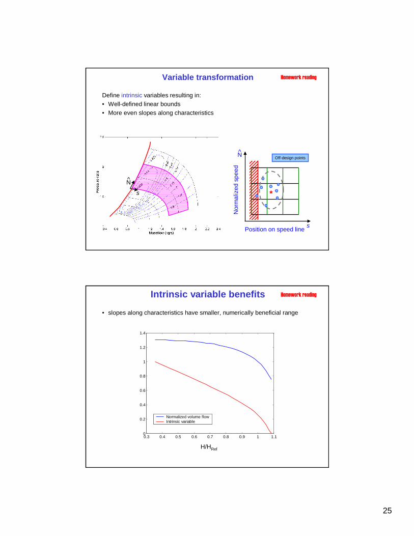
Variable transformation

Define intrinsic variables resulting in:• Well-defined linear bounds• More even slopes along characteristics

Homework reading

H/HRef

0.3 0.4 0.5 0.6 0.7 0.8 0.9 1 1.10

0.2

0.4

0.6

0.8

1

1.2

1.4

Normalized volume flowIntrinsic variable

Intrinsic variable benefits

• slopes along characteristics have smaller, numerically beneficial range

Homework reading

26

0.6 0.7 0.8 0.9 1 1.1 1.2 1.3 1.40

0.1

0.2

0.3

0.4

0.5

0.6

0.7

0.8

0.9

1

DataPoly fit

Bounds: Compressor example

Q/QDes

η/ηmax

η

Req’d compressorpower input

Req’d turbinepower output

Turbine exit temp

-iterate over temp

Solver failure!

Possible pitfalls of polynomial fit:

Homework reading

General problem: optimizers may evaluate use models outside the proper range during the search for the optimum

Bounds on an ideal gas radial turbine

Turbine:Efficiency bound 0.05 < η < 1

Properties:T > 150 K

If T < 150 K, property calculationtruncated at T = 150 K value

Result non-convex, non-physical residual

-2.8 -2.6 -2.4 -2.2 -2 -1.8 -1.6 -1.4 -1.2 -1 -0.8

x 105

0

50

100

150

200

250

300

350

Turbine inlet tempTurbine outlet tempResidual

Homework reading

27

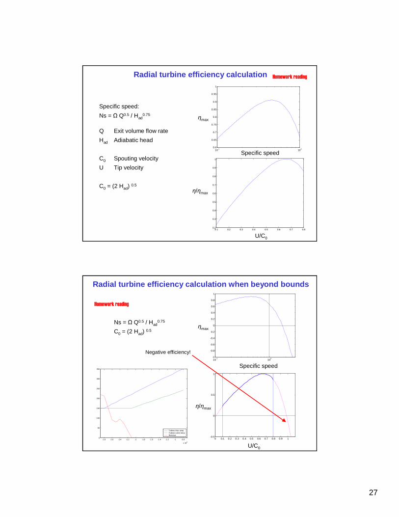
Radial turbine efficiency calculation

0.1 0.2 0.3 0.4 0.5 0.6 0.7 0.80.2

0.3

0.4

0.5

0.6

0.7

0.8

0.9

1

η/ηmax

U/C0

10-1 1000.6

0.65

0.7

0.75

0.8

0.85

0.9

0.95

1

Specific speed

η maxηmax

Specific speed

Specific speed:

Ns = Ω Q0.5 / Had0.75

Q Exit volume flow rate

Had Adiabatic head

C0 Spouting velocity

U Tip velocity

C0 = (2 Had) 0.5

Homework reading

Radial turbine efficiency calculation when beyond bounds

0 0.1 0.2 0.3 0.4 0.5 0.6 0.7 0.8 0.9 1-0.5

0

0.5

1

U/C0

η / η

max

η/ηmax

U/C0

10-1

100

-1

-0.8

-0.6

-0.4

-0.2

0

0.2

0.4

0.6

0.8

1

Specific speed

ηmaxηmax

Specific speed

-2.8 -2.6 -2.4 -2.2 -2 -1.8 -1.6 -1.4 -1.2 -1 -0.8

x 105

0

50

100

150

200

250

300

350

Turbine inlet tempTurbine outlet tempResidual

Ns = Ω Q0.5 / Had0.75

C0 = (2 Had) 0.5

Negative efficiency!

Homework reading

28

A possible solution

-2.8 -2.6 -2.4 -2.2 -2 -1.8 -1.6 -1.4 -1.2 -1 -0.8

x 105

0

50

100

150

200

250

300

350

Turbine inlet tempTurbine exit tempOrig residualImproved residual

Truncate temperature,but extrapolate enthalpy

Bound Ns, U/C0

0 0.1 0.2 0.3 0.4 0.5 0.6 0.7 0.8 0.9 1-0.5

0

0.5

1

U/C0

η / η

maxη/ηmax

U/C0

General rules:• apply bounds to input variable rather than derived quantity• ensure bound implementation robustly produces physical output

for current & surrounding components• test, test and test again

Homework reading

Avoiding Stiffness

• Models with largely varying time scales of the dynamics are called stiff and cause slow-down of the numerical solvers

• Different remedies are possible:– Make a problem non-stiff by using a steady-state

assumption (singular perturbation technique) when the fast dynamics of the system are not of interest.

– Make a problem non-stiff by approximating very slow dynamics with constants.

– Degrease the stiffness by making very fast time constants slower, but keep them approx. 10 times faster than the fastest time scale of interest

29

Stiffness caused by Flow Splitters and Joints (small volumes)

• Many more examples of singular perturbation:– chemical equilibrium– static instead of dynamic momentum balance

Volume3Port Ideal3Port

Pipe

Zero-volume assumption in ideal 3-ports is a singular perturbation

Homework reading

Time scale considerations

• Render a problem less stiff by making the time constants of the fast dynamics slower.

• Different solution for same problem: when to use which solution?– singular perturbation leads to nasty non-linear

equation system– we are not interested in the fast dynamics– even after changing the time constants, the fast

dynamics are much faster than other, interesting dynamics.

30

Easing Stiffness: power plant example

• Very small volumes at tap-off locations cause stiffness– Dynamics of interest: power reserve (several seconds)– making volumes larger by a factor of 100 does not influence the

dynamics of interest (and the dynamics are still much faster than dynamics of interest)

p CV 3

h inp in

m in.

volume 1 volume 2

volume 3

HP - stage

m turbine valve.

m HP - valve.

h CV 1

p CV 1

TCV 1

h CV 2

p CV 2

TCV 2

h CV 3

p CV 3

TCV 3

m HP - stage.

PHP

m stage 1.

Pstage 1

h CV 3

m preheat.

h CV 3p CV 3

mstage 2.

Homework reading

• When non-linear fields are possible inside the components and their resolution is required

• When Underlying Physics is well-understood – will require physics based parameterization (Enabler)

Example : In a vaporizer, if it is known exit gas is saturated, then Xwater (out) = Xsat for lumped model but for distribution of X in the reactor, need to evaluate heat and mass transfer

When to go for distributed Modeling?

x

Temperature

What is max temp? – cannot be resolved by lumped

models, neither by exit temp measurements

Homework reading

31

Best Practices for model development

• Model development• Documentation• Naming Conventions (self-documenting models)• Team development: version control• Testing practices• Robustness metrics

Model Development

• Always assume that somebody else needs to understand and be able to continue work on the model in any phase of the development: document and test while developing (or before), never after the fact.

• Start with simplest models that produces plausible results and test it

• Add complexity one step at a time and test at every step

• Add changes/difficulties and test them one at a time (it is very hard to detect and treat combined difficulties)

• Start with explicit, simple forms, advance towards implicit, numerically challenging ones and test at every step

• Separate the difficulties - e.g., at different stages or in modules

• Build hierarchies of models as in the real systems build moduleshierarchically starting with lowest level modules which provide outputs as elements for higher modules and test every time models are combined

• Adapt models to the needs of the task to be solved, simple models may be sufficient for many tasks

32

Documentation:

• Provide plenty of documentation, in the code and as separate document, provide templates and guidelines for both

• 50% (or more) of the total text should be documentation• Standardize on documentation in model header

– What-how-why of model, assumptions, name, data, test cases, validity range, application areas, qualification level

• Standardize on minimal set of info that has to be added for eachmodel revision, e.g.– Author– Date of change– Reason for change, requester– What has been changed– How it is demonstrated that the revision fixed a problem (name of

test model, verification data set if applicable)

Naming Conventions

• Structuring and naming conventions are influenced by the modeling platform. Models in Modelica are usually structured in small components. Long, self-explaining names help the model reader to understand models, e.g.discharge_saturation_temperature

• Use standardized order of terms, e.g. as inrefrigerant_inlet_temperature

• In Modelica: short names are fine when the meaning is clear from the context, dot-notation can play similar role as long name, e.g:refrigerant_pipe.inlet.Tin addition, variables should always be documented at declaration with a string: parameter Real eta “total turbine efficiency”

33

Team Development

• For any project that involves 2 or more persons, use version control (CVS or similar)

• Team members should present models to each other at regular intervals or, if possible, rotate responsibilities: all team members should be able to work on all models (eXtreme Programming works for modeling, too)

• Naming and coding style conventions should be supported by whole team – simplifies communication

Model Testing

• It is very difficult to overdo component robustness testing (you’ll be bored before that happens!)

• Every model should have an associated test case:– Test model that runs over full range of legal operating conditions

• Testing should be as automatic as possible: use scripts, maybe even in other platform (e.g. matlab scripts to test Dymola-models from matlab in the same way as other matlab code)

• For every model you make, I want to see a test-script that demonstrates the model capabilities – Script that demonstrates failures and limits are also fine.

• Testing must be repeatable: keep original model-generated output data.

• Models mature over time through extended use. – Assign maturity levels e.g. (exploratory, experimentally verified,

production qualified) to models– Verification data that proves the model to achieve a certain level of

predictive capability shall be part of the model library or version control repository

34

Model Robustness Metrics

• Use relevant and difficult tests to check model robustness (e.g. initialize in all corners of operating envelope)

• Robustness criteria depend on model use:– Simulation models should run almost always (e.g. initialization

works in 98% of cases is fine– Optimization models have to be 100% robust, because the model is

called many times during a single run• Robustness problems are almost always due to one of the

numerical pitfalls described earlier on these slides!• High Component-level robustness a necessary precondition for

system level robustness • Option: use many randomized parameters and initial conditions

or Taguchi-test (spans input space in an optimal way)– If all tests are passed, great!– Model robustness is unacceptable if a client-defined percentage of

failures occurs

Homework reading

Model Robustness

• Taguchi tests– Idea: Reduce # of tests by assuming linear

dependence and use orthogonal vectors.– Our result: Testing robustness for 9 input variables

with three levels reduced to 27 experiments.– Experiments implemented as a sequence of steps.– Scenario can be extended and reduced

dependent on # of variables and # of levels.

Homework reading

35

Model Robustness

• Taguchi tests– Example from fuel cell testing: Special

reservoir with test sequences for pressure, temperature and compositions.

Homework reading