structuring dynamic models of exploited ecosystems … · 2015-10-28 · structuring dynamic models...

Structuring dynamic models of exploitedecosystems from trophic mass-balanceassessments

CARL WALTERS1�, VILLY CHRISTENSEN 2 and DANIEL PAULY1, 2

1Fisheries Centre, The University of British Columbia, 2204 Main Hall, Vancouver, BC, Canada V6T 1Z42International Center for Living Aquatic Resources Management, MC PO Box 2631, 0718 Makati City,Philippines

Contents

Abstract page 140Introduction 140From ECOPATH to differential equations 141

The ECOPATH master equationFrom mass balance to a dynamic model

Primary productionPredicting consumptionNumerical Implementation of ECOSIM

General ECOSIM predictions 148Predictions of transient responses to harvest rate changesPrediction of equilibrium regimesTop-predator take-overs

Delay-differential representation of trophic ontogeny 158A two-pool approachBeverton–Holt factorsSimplification by treating population age as a predictor of feeding rateParameter estimationExample of trophic ontogeny effects: should cannibalism cause dome-shapedrecruitment patterns in Lake Victoria Nile perch?

Discussion 164What goes wrong: some limits to ECOSIM predictions

Productivity for low-fecundity speciesOver-optimistic assessments for intermediate predatorsIndeterminate outcomes in complex food websMisleading parameter estimates from assuming equilibrium in ECOPATH

ECOSIM as a tool for adaptive policy designECOSIM in the spectrum of multispecies modelling approaches

Acknowledgements 168Appendix 1: List of symbols used in model development 168References 170

Reviews in Fish Biology and Fisheries 7, 139–172 (1997)

0960–3166 # 1997 Chapman & Hall

�Author to whom correspondence should be addressed. E-mail: [email protected]

s.mondoux

Text Box

Walters, C. V. Christensen and D. Pauly. 1997. Structuring dynamic models of exploited ecosystems from trophic mass-balance assessments. Reviews in Fish Biology and Fisheries 7(2): 139-172.

Abstract

The linear equations that describe trophic fluxes in mass-balance, equilibriumassessments of ecosystems (such as in the ECOPATH approach) can be re-expressedas differential equations defining trophic interactions as dynamic relationships varyingwith biomasses and harvest regimes. Time patterns of biomass predicted by thesedifferential equations, and equilibrium system responses under different exploitationregimes, are found by setting the differential equations equal to zero and solving forbiomasses at different levels of fishing mortality. Incorporation of our approach as theECOSIM routine into the well-documented ECOPATH software will enable a wide rangeof potential users to conduct fisheries policy analyses that explicitly account forecosystem trophic interactions, without requiring the users to engage in complexmodelling or information gathering much beyond that required for ECOPATH. While theECOSIM predictions can be expected to fail under fishing regimes very different fromthose leading to the ECOPATH input data, ECOSIM will at least indicate likelydirections of biomass change in various trophic groups under incremental experimentalpolicies aimed at improving overall ecosystem management. That is, ECOSIM can be avaluable tool for design of ecosystem-scale adaptive management experiments.

Introduction

There is an emerging consensus among fisheries scientists and managers of aquaticresources, that traditional single-species approaches in fisheries management ought to bereplaced by ‘ecosystem management’ – that is, with approaches that explicitly accountfor ecological interactions, especially those of a trophic nature, as well as for other usesof ecosystem resources than for fisheries. There is more to this trend than the obviousconcern that we cannot simply batter away at the parts of an ecosystem as though theseparts were isolated. Taking an ecosystem view also invites the use of other instruments ofmanagement in addition to harvest regulation, such as enhancement of basic productivity,stock enhancement, and provision of physical structure to moderate trophic interactionsby providing refugia for prey in predator–prey interactions, or marine protected areas.

There is, on the other hand, less of a consensus concerning the tools (conceptual andanalytical) that should be used to formalize and study trophic interactions among theelements of fisheries resources systems. Three approaches have gained some ground,but none has received general acceptance. First, there is the detailed approachrepresented by multispecies virtual population analysis (MSVPA, Sparre, 1991), inspiredby the multispecies age-structured population models of Andersen and Ursin (1977).MSVPA utilizes extensive time series of catch-at-age data to produce natural mortalityrates and population estimates for the exploited part of ecosystems. Further it makesprognosis of the impact of changes in fishing intensity, mesh sizes, etc. MSVPA hasbeen applied to only a few systems, but considerable experience has been gained on itsproperties. However, its data intensiveness will preclude its application to manysystems, at least in its original form (but see Christensen, 1996). A second potentiallyuseful class of models are less data-driven, simpler differential equation models forbiomass dynamics, which have a long, if chequered tradition (Larkin and Gazey, 1982).Such biomass dynamics models can be viewed as ecosystem-scale extensions of single-species surplus production models. A third approach has been bioenergetics modelling

140 Walters et al.

to assess at least impacts of changing predation regimes, mainly in freshwaterecosystems (Stewart et al., 1981; Kitchell et al., 1994, 1996).

The major problems with the simulation models, as far as practical application tofisheries resource systems, have been that: (1) they require a high degree of expertiseon the part of the modeller; (2) they are difficult to parameterize by piecemeal analysisof component trophic interactions (trophic models with ‘reasonable’ parameter estimateshave a nasty way of self-simplifying, losing trophic groups due to competitive andpredation interactions), and this parameterization often involves concepts fromtheoretical ecology not familiar to fisheries practitioners; (3) time series data usuallylack adequate contrast in effort and abundance regimes to permit clear discrimination(accurate estimation) of parameters representing intraspecific versus interspecificeffects; and (4) the lack of transparency resulting from (1)–(3), combined with theoccasional output of doubtful results, has tended to prevent ecosystem simulationmodels from being routinely used by fisheries scientists.

A simpler approach for analysis of trophic interactions in fisheries resource systems isthe ECOPATH system of Polovina (1984), further developed by Christensen and Pauly(1992a,b, 1995), and widely applied to aquatic ecosystems (fisheries resource systems,aquaculture ponds and natural systems; see contributions in Christensen and Pauly, 1993),and recently also to farming systems (Dalsgaard et al., 1995). Like bioenergeticsmodelling, ECOPATH has been appreciated by a wide variety of authors as an approachfor summarizing available knowledge on a given ecosystem, to derive various systemproperties and to compare these with the properties of other ecosystems. Also, systematicapplication of ECOPATH has enabled a number of generalizations about the structure andfunctioning of ecosystems, and thus to revisit earlier inferences based on smaller datasets (Pauly and Christensen, 1993, 1995; Christensen, 1995b,c; Pauly, 1996). However,ECOPATH provides only a static picture of ecosystem trophic structure (it answers thequestion: what must trophic flows be to support the current ecosystem trophic structureand be consistent with observed growth and mortality patterns?). This precludes the useof its results for answering ‘what if’ questions about policy or ecosystem changes thatwould cause shifts in the balance of trophic interactions.

Here we present an approach for using the results of ECOPATH assessments toconstruct dynamic ecosystem models, as systems of coupled differential equations thatcan be used for dynamic simulation and analysis of changing equilibria. We show howthis approach, which we call the ECOSIM module of ECOPATH, can be used for studyof fishery response dynamics in any ecosystem for which there are sufficient data toconstruct a simple mass-balance model. We begin with a basic biomass dynamicsformulation in the following section, and present some general results from thisapproach. One of these results is an inadequacy in representation of fishes that showstrong trophic ontogeny, feeding widely across the food web as they grow. We show ina later section how this inadequacy can be corrected by using a more complex delay-differential equation structure that represents numbers/body size dynamics as well asbiomass dynamics.

From ECOPATH to differential equations

Here we first review the mass-balance relationships used in ECOPATH assessment, thenshow how relatively simple biomass dynamics models can be derived from the

Dynamic models of exploited ecosystems 141

ECOPATH results. We point out that these models are likely to give unrealistic resultsunless they include effects of prey behaviour/spatial distribution on availability of prey topredators. We suggest an approach to model dynamics of availability in a way that allowsusers of ECOSIM to generate a range of predictions representing alternative hypothesesabout ‘top-down’ versus ‘bottom-up’ control of trophic interactions. Symbols used in thefollowing presentation are summarized in Appendix 1.

THE ECOPATH MASTER EQUATION

Trophic mass-balance models in ECOPATH are defined by the master equation:

Production of (i) utilized � catch of (i) � consumption of (i) by its predators (1)

where (i) is any functional group within the ecosystem in question, over any period (e.g.a year or a decade), at the end of which the system had the same biomass state as at thebeginning.

Equation 1 can be broken up into its components:

Bi:(P=B)i:EEi � Yi �Xn

j�1

Bj:(Q=B) j:DC ji (2)

where: Bi is the biomass of (i) during the period in question, with the system havingi � 1, . . ., n functional groups; (P=B)i is the production/biomass ratio of (i) equal tototal mortality rate (Zi) under the assumption of equilibrium (Allen, 1971); EEi is theecotrophic efficiency, i.e. the fraction of the production (Pi � Bi:(P=B)i) that isconsumed within the system or harvested; Yi is the yield of (i), i.e. its catch in weight,with Yi � Fi:Bi, where F is the fishing mortality; Bj is the biomass of the consumers orpredators; (Q=B) j is food consumption per unit of biomass for consumer j, and DC ji isthe fraction of i in the diet of j (DC ji � 0 when j does not eat i). Note thatQij � Bj(Q=B) j DC ji is the total consumption of pool (i) by pool j per time.

The parametrization and solving of Equation 2, which leads to trophic flow analysessuch as in Fig. 1, was discussed in Christensen and Pauly (1992a,b), and numerouscontributions in Christensen and Pauly (1993), and need not concern us here, except tomention that it is very straightforward as it allows combining original data withinformation previously published on the various groups included in a system. A recentlydeveloped Monte Carlo routine (‘EcoRanger’) has been added to the Windows versionof ECOPATH, enabling consideration, in a Bayesian context, of uncertainty in the inputdata (Christensen and Pauly, 1995).

FROM MASS BALANCE TO A DYNAMIC MODEL

Here we concentrate on how the system of linear equation in (2) can be re-expressed as asystem of differential equations. At equilibrium we have

0 � Bi:(P=B)i ÿ Fi:Bi ÿ Mo Bi ÿXn

j�1

Qij (3)

where Qij is the amount of (i) consumed by ( j), and Mo is the mortality rate notaccounted for by consumption within the system. Except for primary producers,ECOPATH computes Bi:(P=B)i to be equal to a growth efficiency gi times the food

142 Walters et al.

Fis

hery

cat

ch

Oth

er e

xpor

t

Flo

w to

det

ritus

Res

pira

tion

1234

Trophic level

0.0

0.0

0.0

(0.0

)

Bat

hype

lagi

cs

142.

076

.615

.01.

94.

5 (240

.0)

B

52.

5P

5

50.0

233.

90.

00.

21.

9

(236

.0)

149.

524

0.0

10.0

0.5

Mic

ro-

zoop

lank

ton

Det

ritus

Phy

topl

ankt

on

B5

1.0

P5

400

(25.

0)

15.0

0.0

6.2

1.8

0.1 1.

9

B5

0.02

P5

0.00

2

B5

10.0

P5

5.00

B5

0.5

P5

1.0

(4.7

)0.4

1.0

0.6

B5

0.05

P5

0.06

2.7

0.2

0.5

(0.8

)

Ape

x pr

edat

ors

Epi

pela

gic

nekt

on

Larg

ezo

opla

nkto

n

0.5

0.1

1.7

4.5

0.8

(7.6

)

Mes

opel

agic

s

0.1

0.1

(0.5

)

0.2

B5

1.5

P5

0.11

30.

20.

00.

6

(2.0

)

0.1

1.1

Bet

hnic

fish

Ben

thos

B5

5.0

P5

0.5

B5

2.6

P5

1.56

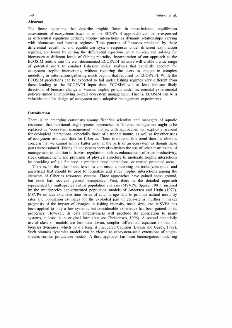
Fig

.1.

Flo

wdi

agra

mof

the

cent

ral

Sou

thC

hina

Sea

pela

gic

ecos

yste

min

the

1980

s,as

cons

truc

ted

usin

gE

CO

PAT

Han

ddo

cum

ente

din

Paul

yan

dC

hris

tens

en(1

993)

.T

hesi

zeof

the

boxe

sis

roug

hly

prop

orti

onal

ofth

elo

gari

thm

ofth

ebi

omas

ses

(B;

tkm

ÿ

2),

whi

leth

ear

row

sdo

cum

ent

the

fate

ofpr

oduc

tion

(P;

tkm

ÿ

2ye

ar

ÿ

1).


consumed by group (i), i.e. trophic flows Qij into consumer pools (i) are computed so asto satisfy Bi:P=Bi � gi

PjQji:

To construct a dynamic model from Equation 3, we must (1) replace the left side ofEquation 3 with rate of biomass change dBi=dt; (2) for primary producers, provide afunctional relationship to predict changes in (P=B)i with biomass Bi, with thisfunctional relationship representing competition for light, nutrients, and space; and (3)replace the static Qij pool-to-pool consumption estimates with functional relationshipspredicting how the consumptions will change with changes in the biomasses Bi and Bj:

Generalizing Equation 3 for both equilibrium and non-equilibrium situations, we have

dBi=dt � f (B)ÿ M o Bi ÿ Fi Bi ÿXn

j�1

cij(Bi, Bj) (4)

where f (B) is a function of Bi if (i) is a primary producer, or f (B) �giPn

j�1 c ji:(Bi, Bj) if (i) is a consumer, and cij(Bi, Bj) is the function used to predictQij from Bi and Bj. If we can provide reasonable predictions of the f (B) and cij(Bi, Bj)functions, the system of Equation 4 can be integrated with Fi varying in time, to providedynamic biomass predictions of each (i) as affected directly by fishing and predation on(i) and changes in food available to (i), and indirectly by fishing or predation on otherpools with which (i) interacts.

Primary production

For primary producers, we propose the simple saturating production relationship

f (Bi) � ri Bi=(1� Bi hi) (5)

where ri is the maximum P=B that (i) can exhibit when Bi is low, and ri=hi is themaximum net primary production rate for pool (i) when biomass (i) is not limiting toproduction (Bi high). Assuming the ECOPATH user can provide an estimate of the ratioof maximum to initial or base P=B (ratio of ri to (P=B)i entered for ECOPATHestimation), ri can then be computed from this ratio, and hi from the ECOPATHbase estimates of primary production rate Bi:(P=B)i and biomass Bi as hi �

[(ri=(P=B)i)ÿ 1]=Bi: Setting ri very large (ratio very large) in this formulation hasthe effect of making primary production rates in the system remain constant atECOPATH estimates independent of primary producer biomasses. It is obviously wise toinclude at least some limitation on primary production rates in the model, to representcompetition among plants for light, nutrients and space. When in doubt about how toquantify this limitation, the conservative choice would be to make production rates verysensitive to biomass and to assume maximum rates ri=hi not much higher than the initialECOPATH rate estimate.

Predicting consumption

Various functional relationships have been proposed in the ecosystem and fisheriesmodelling literature for predicting consumption flows cij(Bi, Bj), to represent predator–prey encounter patterns and physiological-behavioural phenomena such as satiation ofpredators. In fisheries contexts, predation interactions have usually been represented orpredicted from the simple Lotka–Volterra or ‘mass action’ assumption:

144 Walters et al.

cij(Bi, Bj) � aij Bi Bj (6)

where aij represents the instantaneous mortality rate on prey i caused by one unit ofpredator j biomass (contribution to Zi by presence of a unit of consumer j biomass; e.g.Andersen and Ursin, 1977). This ‘catchability’ interpretation of aij corresponds in theecological literature to interpreting aij as the ‘rate of effective search’ (Holling, 1959) ofthe consumer, measured per unit consumer biomass. Equation 6 is convenient from anECOPATH perspective, because every aij can be estimated directly from thecorresponding ECOPATH flow estimate: aij � Qij=(Bi:Bj):

A potential weakness of Equation 6 is that it does not represent satiation bypredators; however, usually we do not view this as a serious issue (but see discussionbelow), because field observation of stomach contents in aquatic ecosystems suggeststhat most consumers are rarely able to achieve satiation (or are unwilling to take thepredation risks necessary to achieve full stomachs most of the time).

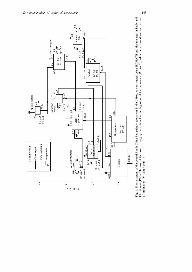
Probably the most serious weakness in the simple mass-action predictor (Equation 6)is that predator–prey encounter patterns in nature are seldom random in space, and aremost often associated with behavioural or physical mechanisms that limit the rates atwhich prey become available to encounters with predators. For example, consider theflow from phytoplankton in the water column to benthic filter feeders; here only asmall fraction of Bi is available to the consumer, that fraction being limited by physicalmixing and sinking processes that bring phytoplankton near the bottom. For otherexamples: zooplankton often show strong vertical migration patterns that limit theiravailability to planktivorous fish; planktivorous fish often spend much of their time inbehavioural (schooling) or spatial (shallow water, holes) refuges that limit theirencounter rates with (or the time they are exposed to) piscivores. In view of howubiquitous these spatial and behavioural limiting mechanisms are, Equation 6 may wellgrossly overestimate the potential for increasing flow to consumer pools when consumerbiomasses increase (e.g. in model scenarios where fishing rates on the consumers aredecreased to test whether the ecosystem could support higher abundances to meet somefishery management objectives). We have chosen in ECOSIM to represent suchlimitations by viewing each prey pool Bi as having an available component to eachconsumer j, Vij, at any moment in time (Fig. 2). This biomass Vij may exchange fairlyrapidly with the unavailable biomass according to the exchange equation:

dVij=dt � vij(Bi ÿ Vij)ÿ vijVij ÿ aijVij Bj: (7)

That is, Vij gains biomass from the currently unavailable pool (Bi ÿ Vij) at rate vij,biomass returns to the unavailable state at rate vijVij, and biomass is removed from Vij

by the consumer at a mass-action encounter rate aijVij Bj: Assuming the exchangeprocess between V and B operates on short time scales relative to changes in Bi and Bj,Vij should stay near the equilibrium implied by setting dV=dt � 0 in the above exchangeequation:

Vij � vij Bi=(2vij � aij B j): (8)

At this equilibrium varies with Bi and Bj, the consumption flow from i to j is thenpredicted to vary as

cij(Bi, Bj) � aijvij Bi Bj=(2vij � aij B j): (9)


For low consumer biomasses, this functional relationship reduces to mass-action flow,c � a9Bi Bj, where a9 is half of the aij value predicted without considering limitation ofprey availability. But for high consumer biomass Bj(aij Bj � 2vij), c approaches amaximum ‘donor controlled’ flow rate c � vij Bi: Thus vij represents the maximuminstantaneous mortality rate that consumer j could ever exert on food resource (i). InECOSIM, parameter estimates for vij and aij in Equation 9 are obtained by having theuser specify an estimate of the ratio of the maximum to the ECOPATH base estimate ofthe instantaneous mortality rate. Given this ratio, say xij, the vulnerability exchange rateis calculated as vij � xijQij=Bi and substituting this estimate into Equation 9 along withECOPATH Qij, Bi, Bj estimates gives aij � 2Qijvij=(vij Bi Bj ÿ Qij Bj): Note here that theestimate aij approaches infinity and becomes negative for ratios approaching 1 or less(i.e. for ratios implying that not even the initial estimated flow Qij could be sustained). Inaddition, Equation 9 can be made to approach the simpler mass-action prediction ofEquation 6 by setting the ratio of maximum to estimated Qij very large.

ECOSIM offers two other functional forms for predicting consumption flows. Thefirst is a simple donor-control option:

cij(Bi, Bj) � vij Bi (10)

which ignores consumer abundance entirely in computing the flow (vij estimated fromECOPATH estimates as vij � Qij=Bi); this option is useful for representing the ‘flow’ ofbiomass between pools representing different life stages of a species or functional group,where i is the pool of younger individuals.

The second is a ‘joint limitation’ relationship intended to approximate flow changesin situations where there is a limit on total flow when either prey biomass or predatorbiomass or both increase to high levels:

cij(Bi, Bj) � aij mij Bi Bj=(mij � aij Bi Bj): (11)

a

Bi

Bj

v

Vi

5 Predator rate of search

5 Total prey biomass

5 Predator biomass

5 Behavioural exchange rate

5 Vulnerable prey biomass

Fast equilibration between Bi 2 Vi and Viimplies Vi5 vBi /(2v1aBj)

Unavailable preyBi 2 Vi

Available preyVi

PredatorBj

aViBj

v(B 2 V)

vV

Fig. 2. ECOSIM approach to simulation of biomass flow between unavailable biomass of prey(Bi ÿ Vi), available biomass of prey (Vi), and flow to predator j with biomass Bj.

146 Walters et al.

This relationship predicts mass-action flow for low Bi and/or Bj, but flow reaching amaximum mij when either Bi or Bj becomes very large (mij estimated by having the userspecify the ratio of mij to ECOPATH estimate of Qij):

Beyond the primary production and consumption relationships defined by Equations2–4, ECOPATH and ECOSIM account for one other basic type of trophic process,namely the production and consumption of detritus. ECOSIM adds at least oneadditional dynamic equation, for detritus biomass. Input rates to this biomass includethe Mo Bi ‘other mortality’ rates not accounted for by consumption within the system,plus the non-assimilated fraction of each consumption flow (default set to 0:2:cij foreach flow from j to i; Winberg, 1956), plus ‘import’ (user defined) of detritus fromsurrounding ecosystems. Losses to the detritus pool (which may include a number ofspecified detritus groups) are cij flows for i � detritus by detritivores (modelled as anyother consumption flows, by Equation 4), plus an export rate edetritus Bdetritus where theinstantaneous export rate edetritus is the value needed to balance detritus biomass gainsand losses when all explicit inputs and outputs are accounted for at ECOPATHequilibrium.

Note that Equations 9 and 11 allow us to represent a strategic range of alternativehypotheses about ‘top-down’ versus ‘bottom-up’ control of trophic structure andabundance (Hunter and Price, 1992; Matson and Hunter, 1992). Setting low values forthe vulnerability ratios vij leads to ‘bottom-up’ control of flow rates from prey topredators, such that increases in prey productivity will lead to prey biomass increasesand then to increased availability to predators. Setting high values for vij leads to ‘top-down’ control and ‘trophic cascade’ effects (Carpenter and Kitchell, 1993); increases intop predator abundance can lead to depressed abundance of smaller forage fishes, andthis in turn to increases in abundance of invertebrates upon which these forage fishesdepend.

Numerical implementation of ECOSIM

Equations 2–4 represent a very modest step towards predicting how ecosystem flowsmight change as biomasses depart from base levels that result in Qij patterns estimatedby ECOPATH. We emphasize that these equations are not likely to apply globally overwide ranges of biomasses. Examples of how they could easily fail for large changes in Bi

and Bj include: (1) limitations on consumer (Q=B) j ratios at high prey densities due tosatiation; (2) explicit switching in foraging strategies by predators when some prey poolBi becomes scarce, to increase encounter rates with other prey types; and (3) changes inprey behaviour or prey pool species/size composition so as to reduce vij when predationrisk (as measured by Bj) increases.

ECOSIM implements two types of numerical assessments using Equations 3–4. First,the user may specify an arbitrary temporal pattern of changes in fishing mortality ratesFi, using a graphical user interface for ‘sketching’ the temporal pattern with thecomputer mouse. The dynamical equations are then integrated to give predicted biomasspatterns over time, using a fourth-order Runge–Kutta numerical integration scheme thathas been tested for numerical stability and accuracy with inputs from a large number ofECOPATH files, including all those listed in Appendix 4 of Christensen and Pauly(1993).

ECOSIM can calculate predicted changes in equilibrium biomasses over a range ofvalues for F for a particular functional group or for a gear type that generates Fs over


several groups. For small increments in F, this procedure predicts marginal or directionsof change in all biomasses due to increasing F on any one group. For wider ranges ofF, the basic ECOSIM output is a graphical display of the relationship betweenequilibrium biomasses, catch and F (an ecosystem version of plotting equilibriumbiomass and catch versus effort or F for surplus production models). The equilibriumprocedure uses a Newton method to search for the zeros of the equation system definedby Equations 3–4. It is not guaranteed to be numerically stable, and in fact often failsto find the equilibria when the vij are large, and the model hence approaches Equation6 form. In such cases, approximate equilibrium solutions and/or cyclic patterns can befound by integrating the equations over time while slowly changing Fs.

A preliminary stand-alone version incorporating these numerical procedures andgraphic routines for interpretation of results is available for testing purposes; thepreliminary ECOSIM module is available through the University of British ColumbiaFisheries Centre home page (http://fisheries.com). Further work is in progress tointegrate the ECOSIM module as a routine of the Windows version of the ECOPATHsoftware (contact the second author: [email protected], or see the ICLARMhome page http://www.cgiar.org/iclarm).

General ECOSIM predictions

A large number of ECOPATH trophic flow applications have been published (over 60data files from around the world are available now for general use and analysis), and wehave run test ECOSIM simulations with 40 of these cases. We have examined questionssuch as the following.

• Are transient predictions (of response over time to experimental harvest disturbances)from ECOSIM very different from the predictions obtained from single-speciesanalysis, when indirect effects propagating through the trophic structure are includedin assessment?

• Do ECOSIM time simulations predict maintenance of the trophic complexitymeasured in ECOPATH, or are many simulated pools lost to competitive/predator–prey interactions that are incorrectly modelled due to oversimplification of theinteractions and mechanisms that permit coexistence in real systems?

• How do ECOSIM predictions of MSY and Fmax compare with predictions fromtraditional single-species analysis, for fish at various trophic levels?

• How sensitive are the ECOSIM predictions to particular assumptions about vij or mij

in the flow functional responses?

PREDICTIONS OF TRANSIENT RESPONSES TO HARVEST RATE CHANGES

ECOPATH has been used primarily for basic biomass estimation and for analysis ofecosystem ‘support services’ leading to fish production. From a ‘bottom-up’ trophicperspective, ECOPATH has been useful in assessing ecological limits to fish production,and in identifying key trophic linkages that are necessary for sustained production.Figure 3 illustrates just how different a set of issues and questions can arise when weexamine system dynamics with ECOSIM. The figure shows sample results for a dynamicsimulation based on Equation 9 for the Gulf of Mexico ecosystem (Browder, 1993) with

148 Walters et al.

Dol

phin

s (0

.01) S

hark

s (0

.1)

(a)

(d)

Cra

bs, s

hrim

ps (

1)

Dem

ersa

l pre

dato

rs (

1)

Bill

fish

(0.0

1)

Tuna

(0.

01)

Pel

agic

pred

ator

s(0

.01)

(b)

(e)

Dem

ersa

l fis

h (1

)

Ben

thos

(10

)

(c)

(f)

Zoo

plan

kton

(1)

Mac

kere

l (0.

1)P

elag

ic fi

sh (

0.1)

Ben

thic

pro

duce

rs (

1)

Det

rius

(100

)

Phy

topl

ankt

on (

100)

1020

300

1020

300

1020

30

Year

001

F (year21)Biomass

Fig

.3.

A30

year

run

ofa

Gul

fof

Mex

ico

ecos

yste

mm

odel

,as

sum

ing

ate

mpo

rary

incr

ease

infi

shin

gm

orta

lity

for

shar

ks;

sim

ulat

ion

base

don

EC

OPA

TH

mod

elof

Bro

wde

r(1

993)

.S

imul

atio

nsas

sum

ehi

ghav

aila

bili

tyof

prey

topr

edat

ors,

i.e.

stro

ng‘t

op-d

own’

cont

rol

inth

eec

osys

tem

.(B

iom

asse

sfo

ral

lgr

oups

are

expr

esse

don

the

sam

ere

lati

vesc

ale;

use

mul

tipl

iers

(in

pare

nthe

ses)

for

com

pari

sons

amon

ggr

oups

.)


the vij set large (high ratios, 40:1, of potential to initial flows for all biomass flowpathways).

Here we simulated the effects of a transient increase in the fishery for sharks,followed by a conservation closure. For simpler ECOPATH models (fewer than a dozenbiomass pools), and/or with low values for the vij to limit vulnerability of lower trophiclevels to predation, ECOSIM generally predicts that such disturbances would befollowed by a return to the original ECOPATH equilibrium on roughly the same timescales as would be predicted by single-species surplus production analysis. But in somecases, and for many tests we have done with models containing many functional groupswhile assuming high vij values, we see a very striking and disturbing pattern in thelong-term dynamic predictions: instead of returning promptly to the original equili-brium, the system undergoes continuing long-term change as interactions propagatethrough the food web. These changes may involve violent biomass explosions andcollapses starting as much as 30 years after the initial system perturbation. Hence,complex trophic interaction and flow structures appear to create system response lagsand potential instabilities on time scales that would not readily be predicted fromsingle-species analysis.

We do not have enough phenomenological experience with long-term dynamics infisheries ecosystems to say whether very disturbing predictions of long response lagsand violent community changes are credible or not. There have certainly been somelarge and unexpected changes in marine ecosystems during this century, but these havebeen largely attributed to ‘bottom-up’ changes in ecosystem support processes such asupwelling and ocean circulation, for instance for the Peru upwelling ecosystem (seecontributions in Pauly et al., 1989). In other cases it is an open discussion if suchmajor ecosystem changes are due to environmental or trophic, fishery-induced impacts,e.g. for the North Sea ‘gadoid outburst’ (Cushing, 1980). Perhaps ECOSIM and othertrophic interaction models will open new directions in the search for explanation ofsuch changes.

The only obvious conditions we have seen in the ECOSIM tests that lead to suchcomplex time dynamics are: (1) high vij, mij values, i.e. strong ‘top-down’ predationeffects and predator–prey linkages; and (2) ‘long’ food chains (three or more trophiclevels above primary producers). Most marine ecosystems would satisfy property (2),while we do not have enough experimental evidence of changes in predation regimes tosay whether condition (1) is common under natural conditions. However, we may argueon evolutionary grounds, and on grounds of ecosystem development that, throughcontinuing colonization and extinction, strong trophic linkages may have given way overeons to linkages with low vij values, allowing relatively large biomass of ‘preys’ tobuild up even in the presence of large predator populations (Pauly and Christensen,1996).

It might be that violent changes as shown in Fig. 3 are associated with unrealisticallylarge predicted changes in consumption per biomass (Q=B) ratios for consumers, e.g.the ‘outbreak’ shown after year 20 in Fig. 2 could be because the model incorrectlypredicts that too much food is available to the expanding group, and too rapid aresponse to this food through the assumption that consumption (and production) areproportional to prey biomass, Bi, as well as to predator biomass, Bj. Indeed, highvalues of potential Q=B would, under natural conditions, represent a ‘vacuum’ wherefood is available to support something. Under such conditions, our general experience

150 Walters et al.

in ecology is that nature will use the opportunity, and move towards a state that mightwell include creatures not originally included in the ECOPATH and ECOSIM models.We cannot of course predict what shape such invasions might take.

As a warning sign in ECOSIM of a simulated condition where the predictions mightbe breaking down due to unrealistic Q=B values, the user interface offers an option toplot predicted Q=B ratios over time. In the example shown in Fig. 2, the predicted Q=Bratios generally did not differ by more than a factor of 2 from the ECOPATH baseestimates, and there was no clear Q=B ‘signal’ to indicate the onset of major changes.

Figure 4 shows how the predictions in Fig. 3 are altered when lower ratios ofmaximum to initial flow are assumed (smaller vij), and when lower ratios are combinedwith the ‘joint limitation’ assumption of Equation 11. We conclude from results likethese that if trophic flows are assumed to be limited by prey vulnerability and/orpredator limitation mechanisms, resulting predictions of short-term transient responsewill be quite sensitive to the particular form of model used to represent the flowlimitation. In particular, assuming bottom-up control of flows is likely to lead to overlyoptimistic predictions of recovery and stabilization patterns. Natural ecosystems mostlikely have a mixture of low-vij and high-vij ‘linkages’, i.e. weak and strong predationlinkages; we have not yet explored the consequences for ECOSIM predictions ofassuming various mixtures or distributions of linkage strength, nor have we attempted toquantify the trade-off relationship that likely exists between vij and other parameterslike aij (presumably increasing rates of search for prey as measured by aij necessarilyresults in greater vulnerability to predators as measured by vij).

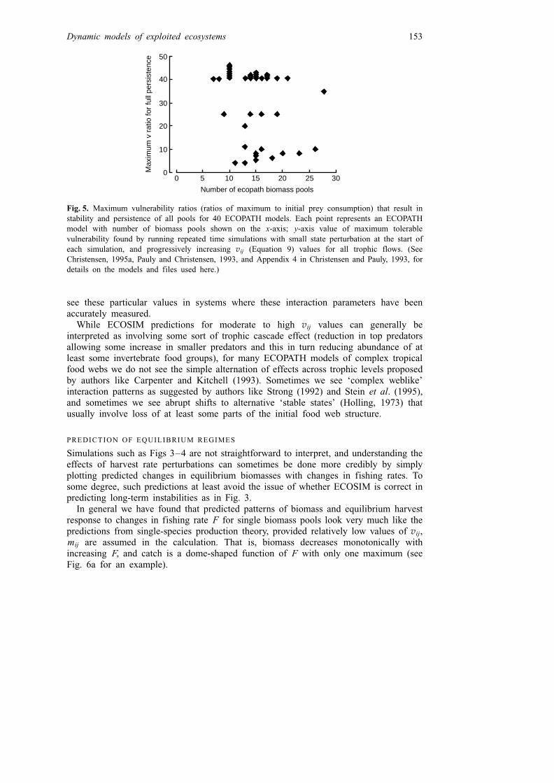
In a systematic examination of time dynamics for 40 ECOPATH models, we foundthat competitive or predator–prey exclusion of one or more functional groups after anarbitrary fishing disturbance (indicating the initial ECOPATH equilibrium to bedynamically unstable) occurred in roughly half the cases (Fig. 5) when vij, mij were setat high values (to allow 40 3 or more of initial flow rates at maximum). For all ofthese cases, restriction of flow rates (to lower ratios of maximum to initial rates for allgroups simultaneously) led to persistence of all groups, and in only a few worst-casesituations was it necessary to restrict the ratio of maximum to initial flow to as low as4.0.

Surprisingly, there was no strong relationship between number of ECOPATH groupsand tendency for the models to self-simplify. The worst case was in fact a very simplymodel of Lake Victoria, which had separate functional groups for cichlids, but whichdid not represent the resource partitioning (as separate groups) that apparently allowscompetitive coexistence of numerous cichlid species (Fryer and Iles, 1972). In thisworst case, a low vulnerability ratio (maximum to initial flow of 4) did result insimulated coexistence, essentially by forcing a partitioning and limitation in the flowfrom the shared food pool at rates low enough to prevent any one cichlid type fromdriving food density low enough to exclude the other types.

The two largest ECOPATH models for which relatively accurate diet compositiondata were used (North Sea model of Christensen, 1995a, and Virgin Islands coral reefmodel of Opitz, 1993) did not exhibit self-simplification even for very high vij values.This suggests the very interesting possibility that strong interactions do occur even incomplex situations, but lead to a sorting process (colonization/extinction/coevolution)such that what finally persists long enough to be studied as an ‘equilibrium’ in the fieldis a very peculiar or particular set of interaction parameter values. Perhaps we can only


010

2030

010

2030

Dol

phin

s (0

.01)

Sha

rks

(0.1

)

Dem

ersa

l pre

dato

rs (

1)

Cra

bs, s

hrim

ps (

1)

Tuna

(0.

01)

Bill

fish

(0.0

1)P

elag

ic p

reda

tors

(0.

1)

Dem

ersa

l fis

h (1

)

Ben

thos

(10

)

Zoo

plan

kton

(1)

Mac

kere

l (0.

1)

Pel

agic

fish

(10

)

Ben

thic

pro

duce

rs (

1)

Det

ritus

(10

0)

Phy

topl

ankt

on (

10)

Year

(a)

(d)

(b)

(e)

(c)

(f)

1020

30001

F (year21)Biomass

Fig

.4.

Eff

ects

onth

eG

ulf

ofM

exic

om

odel

pred

icti

ons

inFi

g.3

ofas

sum

ing

stro

ngli

mit

atio

nof

avai

labi

lity

ofpr

eyto

thei

rpr

edat

ors

(str

ong

‘bot

tom

-up’

cont

rol)

usin

glo

wva

lues

ofv

inE

quat

ion

9,i.e

.vu

lner

abil

itie

sse

tto

gene

rate

max

imum

pred

atio

nm

orta

lity

rate

seq

ual

to3

tim

esth

ein

itia

lE

CO

PAT

Heq

uili

briu

mes

tim

ates

.(B

iom

asse

sfo

ral

lgr

oups

are

expr

esse

don

the

sam

ere

lati

vesc

ale;

use

mul

tipl

iers

(in

pare

nthe

ses)

for

com

pari

sons

amon

ggr

oups

.)

152 Walters et al.

see these particular values in systems where these interaction parameters have beenaccurately measured.

While ECOSIM predictions for moderate to high vij values can generally beinterpreted as involving some sort of trophic cascade effect (reduction in top predatorsallowing some increase in smaller predators and this in turn reducing abundance of atleast some invertebrate food groups), for many ECOPATH models of complex tropicalfood webs we do not see the simple alternation of effects across trophic levels proposedby authors like Carpenter and Kitchell (1993). Sometimes we see ‘complex weblike’interaction patterns as suggested by authors like Strong (1992) and Stein et al. (1995),and sometimes we see abrupt shifts to alternative ‘stable states’ (Holling, 1973) thatusually involve loss of at least some parts of the initial food web structure.

PREDICTION OF EQUILIBRIUM REGIMES

Simulations such as Figs 3–4 are not straightforward to interpret, and understanding theeffects of harvest rate perturbations can sometimes be done more credibly by simplyplotting predicted changes in equilibrium biomasses with changes in fishing rates. Tosome degree, such predictions at least avoid the issue of whether ECOSIM is correct inpredicting long-term instabilities as in Fig. 3.

In general we have found that predicted patterns of biomass and equilibrium harvestresponse to changes in fishing rate F for single biomass pools look very much like thepredictions from single-species production theory, provided relatively low values of vij,mij are assumed in the calculation. That is, biomass decreases monotonically withincreasing F, and catch is a dome-shaped function of F with only one maximum (seeFig. 6a for an example).

0 5 10 15 20 25 30

Number of ecopath biomass pools

0

10

20

30

40

50

Max

imum

v r

atio

for

full

pers

iste

nce

Fig. 5. Maximum vulnerability ratios (ratios of maximum to initial prey consumption) that result instability and persistence of all pools for 40 ECOPATH models. Each point represents an ECOPATHmodel with number of biomass pools shown on the x-axis; y-axis value of maximum tolerablevulnerability found by running repeated time simulations with small state perturbation at the start ofeach simulation, and progressively increasing vij (Equation 9) values for all trophic flows. (SeeChristensen, 1995a, Pauly and Christensen, 1993, and Appendix 4 in Christensen and Pauly, 1993, fordetails on the models and files used here.)


(a)

(c)

(b)

(d)

(f)

(e)

Epi

pela

gic

nekt

on (

1)

Cat

ch

Ben

thic

fish

(1)

Inve

rteb

rate

ben

thos

(10

)

Ape

x pr

edat

ors

(0.1

)

Juve

nile

ape

x pr

edat

ors

(0.0

1)

Mic

rozo

opla

nkto

n (1

)

Zoo

plan

kton

, lar

ge (

10)

Mes

opel

agic

s (1

)

Bat

hype

lagi

cs (

0.01

)

Det

ritus

(10

)

Phy

topl

ankt

on (

1)

0.0

0.5

1.0

1.5

2.0

0.0

0.5

1.0

1.5

2.0

0.0

0.5

1.0

1.5

2.0

Fis

hing

mor

talit

y ra

te (

F; y

ear2

1 )

Relative change

Fig

.6.

Pre

dict

edeq

uili

briu

mre

lati

onsh

ipbe

twee

nfi

shin

gm

orta

lity

onla

rge

pela

gic

pisc

ivor

es,

catc

h(a

rbit

rary

wei

ght

unit

s),

and

pool

biom

asse

sfo

rth

eO

CE

AN

SC

Sm

odel

used

tote

stE

CO

PAT

H(s

eeFi

g.1)

,bu

tw

ith

the

apex

pred

ator

pool

(�

tuna

s)sp

lit

into

mai

nly

zoop

lank

tivo

rous

juve

nile

and

mai

nly

pisc

ivor

ous

adul

tco

mpo

nent

s,w

ith

subs

eque

ntad

just

men

tof

the

P

=

Bs

and

Q

=

Bs:

Inth

isca

se,

the

ecos

yste

m-l

evel

pred

icti

onof

catc

hve

rsus

Ffo

r‘t

unas

’lo

oks

muc

hli

kecl

assi

cpr

edic

tion

sba

sed

onsi

ngle

popu

lati

onpr

oduc

tion

theo

ry.

(Bio

mas

ses

for

all

grou

psar

eex

pres

sed

onth

esa

me

rela

tive

scal

e;us

em

ulti

plie

rs(i

npa

rent

hese

s)fo

rco

mpa

riso

nsam

ong

grou

ps.)

154 Walters et al.

Assuming pure donor control usually results in unrealistic, asymptotic increase incatch with increasing F. The F value generating MSY is, as would be expected,generally lower for top predators (piscivores) than for smaller species like planktivores.Typical Fmsy for top predators are on order 0.3–0.6 yearÿ1, a bit higher than indicatedby many recent single-species analyses but not very unrealistic. Typical Fmsy forplanktivores (e.g. pelagic clupeoids) are on order 0.4–0.8 yearÿ1, again generally higherthan suggested by recent fisheries experience (Patterson, 1992).

A difference for planktivores from single-species modelling is that ECOSIM oftenpredicts no biomass decrease at all as planktivore F is increased from low to moderatelevels. The model predicts instead that this decrease in net planktivore productivityshould be transmitted up the food chain into decreases in top predator biomass (whichin turn reduces the predation mortality rates for planktivores, and allows them to sustainhigher fishing mortalities than would be predicted from single-species theory). Forhigher levels of F, ECOSIM predicts a sharp drop in biomass and catch, when predatorlevels become low.

For larger ECOPATH models (15� pools) and high vij, mij values, the ECOSIMpredictions of equilibrium response to fishing mortality become much more complex.As an example, Fig. 7 shows predicted changes in equilibrium biomasses of allfunctional groups, and catch of engraulids (anchovies), in San Miguel Bay, Philippines(A. Bundy, UBC, PhD in prep.), when only the fishing mortality on the engraulids ischanged. This is compared to a case where fishing mortality by all gears in the bay isvaried simultaneously. In both cases, whether or not the change in fishing patterns iscomplex, the equilibrium biomass relationship to F for engraulids is not a simplemonotonic decrease. The predicted single-species yield relationship has a single peak,but the group is not predicted to persist at all (it is outcompeted by other planktivores,and hit heavily by large predators) under conditions where all fishing mortalities in theecosystem are reduced. Zooplanktonic leiognathids, a similar trophic group in thismodel, are also predicted to be very rare in the absence of fishing, and further to evenhave a yield relationship with two peaks (two Fs that give high catch; not shown inFig. 7).

We have seen quite a number of complex relationships like these, and we have beenunable to generalize about expected patterns of response. Under high vij, mij

assumptions, there are strong feedbacks both up and down the food web as fishingmortalities are changed, and the net impact of changes in predation and competitionregimes on each biomass pool appears to be quite unpredictable (except for largepiscivores, which profit mightily in most models from reduction in fishing mortality).

As in time-transient cases, we simply cannot say at this time whether predictions ofviolent changes in equilibrium biomass patterns under changing fishing regimes areunrealistic. Some of the common predicted changes, such as large increases in biomassand production of prawns in tropical cases, accord in a general way with fisheriesdevelopment experience (Gulland and Garcia, 1984). But very often ECOSIM predictssubstantial simplification of ecosystems, through dominance by large predators, whenfishing is substantially reduced. It is certainly not a matter of common wisdom infisheries that reducing fishing might actually lead to reduced diversity at lower trophiclevels. The development of marine refuges around the world promises to offer excellentopportunities to test this prediction and to gain experience needed to set more realisticvalues for parameters that limit the strength of top-down trophic effects (vij, mij).


TOP-PREDATOR TAKE-OVERS

Novice ECOPATH users are encouraged to work with and develop a simple pelagic foodweb model, for which estimation results are distributed with the program (OCEANSCSdata file). This model represents flows from primary production through plankton toplanktivorous fish to a tuna-like piscivore. When this model is run in ECOSIM with highvij or mij values (maximum flows 33 or more the initial ECOPATH Qijs), and whenequilibrium analysis is used to predict the effect of reducing F on the piscivore, apathological prediction occurs.

The piscivore builds up dramatically in abundance, as might be expected if it werebeing fished hard in the ECOPATH base situation. But as it builds up, its main food

Zooplankton (1)

Detritus (10)

Phytoplankton (10)

Sergestidae (1)

Penaeidae (1)

Sciaenidae (1)

Demersal feeders (1)

Large crustaceans (1)

All gears

Engraulids only

(a) (b) (c)

(h)(g)(f)

0.0 1.0 2.0 0.0 1.0 2.0 0.0 1.0 2.0

0.0 2.5 5.0 0.0 2.5 5.0 0.0 2.5 5.0

Fishing mortality rate (F; year21

)

Equ

ilibr

ium

bio

mas

s an

d ca

tch

ZB Leiognathidae (1)

Pelagics (1)

Engraulidae (1)

ZP Leiognathidae (0.1)

Fig. 7. Predicted equilibrium relationship between fishing mortality (by all gears in upper panels, andby gears targeting engraulids in lower panels), biomass by group, and engraulid catch (arbitrary weightunits) in San Miguel Bay, Philippines. (Biomasses are expressed on the same relative scale; usemultipliers (in parentheses) for comparisons among groups.) Note that the engraulids are predicted tohave a low biomass in the natural system, i.e. when F for all gears is low (panel c). Such complexresponse predictions are not unusual in ECOSIM representations of smaller fishes in tropical trophicwebs.

156 Walters et al.

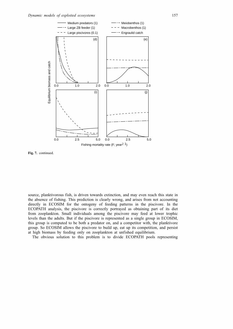
source, planktivorous fish, is driven towards extinction, and may even reach this state inthe absence of fishing. This prediction is clearly wrong, and arises from not accountingdirectly in ECOSIM for the ontogeny of feeding patterns in the piscivore. In theECOPATH analysis, the piscivore is correctly portrayed as obtaining part of its dietfrom zooplankton. Small individuals among the piscivore may feed at lower trophiclevels than the adults. But if the piscivore is represented as a single group in ECOSIM,this group is computed to be both a predator on, and a competitor with, the planktivoregroup. So ECOSIM allows the piscivore to build up, eat up its competition, and persistat high biomass by feeding only on zooplankton at unfished equilibrium.

The obvious solution to this problem is to divide ECOPATH pools representing

0.0 2.5 5.0

(d)

0.0 1.0 2.0

Fishing mortality rate (F; year21)

Equ

ilibr

ium

bio

mas

s an

d ca

tch

(e)

(i) (j)

0.0 2.5 5.0

Medium predators (1)

Large piscivores (0.1)

Large ZB feeder (1)

Meiobenthos (1)

Engraulid catch

Macrobenthos (1)

0.0 1.0 2.0

Fig. 7. continued.


species with broad ontogenetic changes in diet into a series of life stage pools withbiomass moving directly between pools using a donor-controlled flow calculation.However, it is not obvious how to correctly set parameter values for such flows; if thevalues are not set correctly, life stage pools may ‘take off’ on their own, reachinghigher biomasses than would actually be possible, and end up acting as competitorsrather than parts of a single population. Ultimately, the only safe answer is to model theinternal size/numbers structure of pools properly, using concepts and methods extendedfrom single-species analysis; this extention of the biomass dynamics model is presentedin the next section.

Delay-differential representation of trophic ontogeny

A TWO-POOL APPROACH

A simple solution to the problem of dealing with trophic ontogeny, especially for toppredators, would be to divide each group into two (sub-)groups representing the juvenileplanktivore/benthivore stage, and the adult stage. But we cannot apply purely biomass-related consumption/mortality rules, following Equation 4 above, to the dynamics of eachof such groups with an added linkage representing maturation flow from juvenile toadult. With no constraint on the two groups besides biomass flow due to ‘graduation’from the juvenile to the adult group, the groups would generally show unrealistic biomassdynamics.

BEVERTON – HOLT FACTORS

ECOSIM deals with this problem by allowing users to specify a two-pool delay-differential model structure that simultaneously accounts for numbers of fish in thegroups as well as their biomasses. Numbers are included in the model because they‘constrain’, and are better predictors of, food consumption rates (predicted Q). Inessence, we require that the ‘adult’ pools for top predators receive numbers of recruits aswell as biomass from ‘juvenile’ pools, and that the juvenile pools in turn receive numbersof recruits from the adult pools.

In two-pool cases, we allow the user to replace flow functions like Qij � aij Bi B j withQij � aij Bi N j or Qij � Bi A j where N j is number of predators in pool j and A j is the‘total age’ (Equation 7 below) of these predators. This predator number or total ageproportionality rather than predator biomass proportionality is easily justified.

Assume that predator food consumption per individual of age a, (dQ=dt)a, varieswith age approximately as suggested by Pauly (1986) and Temming (1994a,b):

(dQ=dt)a � Æ[1ÿ exp (ÿKa)]2 (12)

where Æ is maximum body weight and K is the von Bertalanffy growth parameter. Thentotal consumption rate Q integrated over age will vary as

Q �

�

aNa(dQ=dt)a da � Æ

�

aNa ÿ 2

�

aNa eÿKa

�

�

aNa eÿ2Ka

� �

: (13)

We can write Equation 13 more compactly by calling each of the three integrals onthe right side of (13) a ‘Beverton–Holt factor’ N (m), defined simply by

158 Walters et al.

N (m)�

�

aNa eÿm Ka for m � 0, 1, 2 (14)

so that Q � ÆfN (0)ÿ 2N (1)

� N (2)g: Note here that N (0) is simply the number of animals

in the pool. If individuals recruit continuously to N at rate Rt per time (this rate need notbe constant), if these individuals are subject to total mortality rate Z, and if they leavethe pool after time T (to die or enter another pool as, say, adults), then the Beverton–Holt factors can be found by solving the simple differential equations

dN (m)=dt � Rt ÿ RtÿT eÿ( Z�m K)T

ÿ (Z � mK)N (m), m � 0, 1, 2: (15)

This very remarkable result was first found by Cooke (1983). If Equations 15are accompanied by a fourth biomass equation of the general form dB=dt �wk Rt ÿ w0 RtÿT � gQÿ (Z � 3K)B, the resulting system of four equations will exactlymimic the behaviour of the Beverton–Holt dynamic pool model with continuousrecruitment and knife-edge entry to the pool at size w0 (and exit from the pool at sizewk). This is a delay-differential equation (continuous time) analogue of the delay-difference equations for B and N derived by Deriso (1980) and Schnute (1987) using asimpler growth model. In other words, by solving Equations 15 for each group alongwith the biomass equation, we can in principle make ECOSIM behave exactly like a setof Beverton–Holt dynamic pool models, with trophic linkages included throughECOSIM predictions of Q and Z. For this we should have Æ Equation 13 include preydensity effects (Æ � aij Bi or aijVij), and Z be the sum of mortalities due to allconsumers/fisheries. This then would require solving four differential equations ratherthan two for each ECOSIM functional group.

SIMPLIFICATION BY TREATING POPULATION AGE AS A PREDICTOR OF FEEDING RATE

Equation 15 leads to an unnecessary explosion in the number of differential equations tobe solved when ECOSIM is faced with many juvenile–adult paired pools. We avoidunnecessary complication by noting, following Pauly (1986), that Equation 12 impliesthat food consumption rate varies almost linearly with age over the range of ages whichcontributes most to the consumption within groups. Hence, if consumption per predatoris proportional to age for constant food density Bi, the rate of effective search aija for agea predators is about proportional to age also. Adopting this simplification and integratingconsumption rates over numbers of fish by age then gives

Qij �

�

aNa(dc=dt)a da �

�

aNasaBi � sBi Na (16)

where N denotes total numbers over all ages and rate of effective search aija is set toaija � sa with s being the slope of the feeding rate–age relationship. So Q will act asaij:B:N with aij � s:a (mean age). For juveniles, mean age should not vary greatly unlessthere are violent changes in mortality rate. For adults where we may wish to examinepolicies that could cause mean age to vary greatly, we replace N with total adult age:

A ��

aaNa da and Qij � aij Bi A j: (17)

We can write a simple differential equation for the time behaviour of A just as we canfor the Beverton–Holt factors in Equation 15. Using that method, the delay differential


equation model for any juvenile–adult pair of ECOPATH groups in ECOSIM is thengiven by five differential equations, here shown for a single species with subscript Jdenoting the juvenile (planktivore/benthivore) stage and A the adult stage:

dBJ=dt � gQJ ÿ ZJ BJ � Rw0 ÿ wk RtÿT exp fÿZJTg (18)

dNJ=dt � Rt ÿ RtÿT exp fÿZJTg ÿ ZJ NJ (19)

dBA=dt � wk RtÿT exp fÿZJTg ÿ Rtw0 � gQA ÿ ZA BA (20)

dNA=dt � RtÿT exp fÿZJTg ÿ ZA NA (21)

dA=dt � TRtÿT exp fÿZJTg � NA ÿ ZA A (22)

Here the biomass rate equations for BA and BJ are as described in previous sections.Zs represent all loss components, and each Qij prey consumption component of Q ispredicted using N j or A j rather than Bj in Equations 6, 9 and 10. Added termsinvolving recruitment R represent biomass flows from adults to juveniles (Rw0 with w0

being an initial juvenile body weight) and graduation from juvenile to adult groupings(wk RtÿT exp fÿZJTg terms, with wk being body weight at graduation, and T being theage at which body weight wk is reached and graduation takes place). The numbersdynamics equations are just recruitment rates less mortality rates. Here R represents thenumber of new recruits to juvenile numbers NJ per unit of time, and in ECOSIM weassume R � b:BA, i.e. no density dependence in production of early juveniles (brepresents juveniles produced per unit adult biomass per time; assumption here is thatfecundity per unit adult biomass stays constant, which does not preclude densitydependence in juvenile survival and/or indirect density dependence through effects onadult biomass).

For precise prediction in scenarios where varies ZJ varies greatly over time, weshould in principle replace ZJ in the exp fÿZJTg of Equations 18–22 with the timeintegral of ZJ over time from t ÿ T to t. However, our experience with test ECOPATHmodels and a variety of time-varying policies is that this integral generally changesslowly relative to T, because the predators that generate ZJ generally have slowerdynamic responses than the smaller juveniles that they eat. This means that the currentvalue of ZJ at any moment in a time simulation is a good ‘predictor’ or index of the ZJ

integral over recent time (back to lag T), and the integral need not be stored duringsimulations.

PARAMETER ESTIMATION

Equations 18–22 appear to pose a formidable parameter estimation problem. But inpractice this estimation can be simplified greatly if we assume to begin with thatRw0 � wk RtÿT exp fÿZJTg at the initial ECOPATH equilibrium, i.e. at initialequilibrium the reproductive ‘investment’ Rw0 by adults just balances gain to adultbiomass from the investment. Under this assumption, the ECOPATH user can proceedwith estimation of Bs, Qs, and Zs without having to deal explicitly with the graduationflow between juvenile and adult groups. We find this reasonable as calculations fortypical growth/survival rates and wk values indicate this flow will generally be smallcompared with other flows, in any case.

The user need only specify wk and W1

, which we use to calculate R by thefollowing steps:

160 Walters et al.

1. substituting ZA into the Beverton–Holt equation for mean adult body weight(Beverton and Holt, 1957; e.g. equation (6) in Hoenig et al., 1987);

2. using this mean body weight to calculate adult numbers (NA � BA=mean weight);3. computing adult recruitment rate needed to balance ZA(RtÿT exp fÿZJTg � ZA NA

at initial ECOPATH equilibrium, so initial R � ZA NA=exp fÿZJTg); and4. calculat ing init ial juvenile numbers at ECOPATH equil ibrium as

NJ � R(lÿ exp fÿZJTg)=ZJ:

In this procedure, we take w0 to be whatever ‘effective entry weight’ is needed to makeRw0 equal to the biomass graduation rate wk RtÿT exp fÿZJTg:

Density-dependence in juvenile mortality rates can be represented in the delay-differential structure by having the time spent in the juvenile stage be variable aroundan initial value given by

Tk � 1=K:ln [1ÿ (wk=W1

)1=3] (23)

which is the age, k, at which fish reach weight wk given von Bertalanffy parameters Kand W

1. In particular, one simple option is to assume

T � (Tk Q0=N0)NJ=QJ, (24)

i.e. juvenile time needed to reach size wk proportional to feeding rate. This option givesT � Tk when the food consumption rate per juvenile is at its base or ECOPATH initialvalue (Q0=N0): Time T then increases whenever either NJ increases above N0 without Qj

increasing, or vice versa. Equation 24 gives density- and food-dependent juvenilemortality, and thus provides an ecosystem-linked recruitment model. It is based on theWerner and Hall (1988) and Walters and Juanes (1993) models, which propose thatjuveniles must spend more time foraging (and hence exposed to predation with totalmortality rate ZJ) as juvenile density increases (see also Jones, 1982).

The parameter estimation procedure outlined above is not necessarily consistent withthe Equation 23 estimate of Tk : An alternative and more robust estimation procedure isto begin by asking the ECOPATH user to provide estimates of wk and Tk , along withthe Bs and Qs. Assuming roughly linear growth in weight for juveniles results in therelation

wk � w0 � gQJ=NJTk, (25)

i.e. growth rate for weight is growth efficiency, g, times consumption per individualQJ=NJ: Given the ECOPATH values for QJ, NJ and ZJ, we first compute w0 as above(assume w0 � wk exp (ÿZJT0)), then solve Equation 25 for NJ: Taking this NJ to be anECOPATH equilibrium, it must satisfy NJ � R[1ÿ exp (ÿZJT0)]=ZJ, which we cansolve for R. Then finally we solve for NA from the initial equilibrium relationNA � R exp (ÿZJT0)=ZA, where ZA is given by ECOPATH. This alternative estimationprocedure guarantees that simulated juveniles will reach weight wk after time T0 whilefeeding at rates estimated from ECOPATH rather than the rates implicit in the growthEquation 23 estimate of Tk : However, there is a hidden price to be paid by following thisprocedure: it may produce an initial adult body size BA=NA that is not consistent withavailable data on W

1and ZA, i.e. the estimates may not agree with mean size estimated

from the Beverton–Holt formula. In such cases a diagnostic will be output by theECOSIM to assist user in reexamination of data and methods used to estimate QJ, QA, c


and BA, as these parameters may be inconsistent with the growth pattern implicit inECOSIM.

EXAMPLE OF TROPHIC ONTOGENY EFFECTS: SHOULD CANNIBALISM CAUSE DOME-

SHAPED RECRUITMENT PATTERNS IN LAKE VICTORIA NILE PERCH?

The Nile perch, Lates niloticus, introduction to Lake Victoria, Central Africa, led tomassive changes in the lake’s endemic fish fauna. There has been little hope for thepersistence of the unique natural cichlid community. However, Kitchell et al. (1996)argue that high fishing rates on the Nile perch may allow at least some components ofthe cichlid fauna to persist and hopefully recover. In a caveat to their predictions basedon bioenergetics modelling and constant recruitment rates to the Nile perch population,Kitchell et al. (1996) warn that because the Nile perch is highly cannibalistic, reductionsin adult stock could well allow substantial increases in juvenile abundance (dome-shapedrecruitment relationship). Juvenile increases could in turn lead to complex, unstabledynamic patterns or at least cancellation of the effect of reducing adult density.

Lates niloticus (10)

Lates niloticus, juv. (10)

Other Oreochromis spp. (1)

Oreochromis niloticus (100)

Bagrus/Clarias (10)

Protopterus (10)

Zooplankton (10)

Caridina nilotica (10)

(a) (b)

(e) (f)Bio

mas

s

0 10 20 30 40 0 10 20 30 40

Year

0

2

F (

year

21 )

Fig. 8. Predicted effects of fishing down the adult Nile perch, Lates niloticus, in Lake Victoria,Africa, then allowing the population to rebuild in a repeat of its introduction. Note how Caridina andRastrineobola stabilize at lower levels, then actually decrease for some time following reduction infishing, before they increase later in the simulation. (Biomasses for all groups are expressed on thesame relative scale; use multipliers (in parentheses) for comparisons among groups.)

162 Walters et al.

We used an ECOSIM model based on ECOPATH models for the Kenyan sector ofthe lake (Moreau, 1995) to examine Kitchell et al.’s concern about cannibalism. TheNile perch pool was split into juvenile and adult components with N-B-A dynamics asin Equations 18–22. Our basic prediction (Figure 8) is essentially the same as that ofKitchell et al. We do not predict large increases in juvenile abundance if the adult Nileperch stock is fished more heavily, nor do we predict that recruitment would increase ordecrease greatly if adult density were allowed to increase. That is, we predict arecruitment relationship of the Beverton–Holt form. This prediction nicely illustratesthe substantial difference between ecosystem and single population dynamic theory.Single population theory, accounting only for changes in cannibalism rate, wouldpredict a dome-shaped recruitment curve. With ECOSIM, we predict instead thatincreases in adult density would lead instead to increased density of foods available tojuveniles (especially the freshwater shrimp Caridina), which would allow juveniles togrow faster and hence reduce time exposed to the cannibalism risk. This is a trophiccascade effect: increasing adult density is predicted to lead to decreases in density of

Haplochromis predators (1)

Mormyrids/Synodontids (1)

Rastrineobola (10)

Insects/mollusks (1000)

Haplochromis benthic feeders (1)

Haplochromisphytoplanktivores (1)

Benthic producers (10)

Phytoplankton (10)Detritus (1000)

0 10 20 30 40 0 10 20 30 40

Year

Bio

mas

s

(c) (d)

(g) (h)

0

2

F (

laye

r21 )

Fig. 8. continued.


cichlids and other competitors/predators of the juveniles, and this in turn to improvedfeeding conditions for the juveniles (and reduced predation risk from the cichlidcommunity). Perhaps this is why in general we do not see strikingly dome-shapedrecruitment relationships in large piscivorous fish: they eat the babies, but they also eatthe competition.

When we reduce adult Nile perch densities to very low levels in the ECOSIM model,which allows the simulated cichlid community to recover as predicted by Kitchell et al.,we predict that Caridina densities should fall from the 1985 level of around 5.9 t kmÿ2

to around 2.9 t kmÿ2. An ECOPATH analysis for the 1971 situation, when the Nileperch stock was still very low, estimated Caridina density at 2.6 t kmÿ2. Thus ECOSIMis successful at predicting not only the direction of the trophic cascade effect onCaridina abundance, but also the magnitude of this response (note that the ECOSIMmodel used only data from the 1985 ECOPATH analysis, not from both 1971 and 1985analyses). ECOSIM also correctly predicts the massive increase in the cyprinidRastrineobola argentea that followed the Nile perch introduction (Ogutu-Ohwayo, 1990,1993).

Discussion

We initiated the development of ECOSIM with a view to providing a very simplebiomass dynamics models. As we began to test this approach, we found it useful toinclude two complications that have not previously been incorporated into multispeciesbiomass models: (1) the notion of vulnerable prey pools (Vij) which can act to limit top-down predation effects; and (2) the use of delay-differential equations to modelpopulation properties besides biomass (N, A). We believe that each of these extensionswill be deserving of future modelling and empirical research on its own. In particular,there is an exciting possibility of developing Beverton–Holt dynamic pool models thatare fully coupled to ecosystem context through variable growth and natural mortalityrates. However, it is by no means clear that this coupling is best or necessarily done justby embedding the dynamic pool model in a larger whole ecosystem model with manyuncertain parameters and feedback relationships. The Lake Victoria example suggestsstrongly that much is to be learned from looking at least two trophic levels away frompredatory species of direct management interest, i.e. we should not treat ‘lower trophiclevels’ as constant just because we do not have fisheries data on them. But perhaps wecan gain such perspectives without developing detailed ecosystem models.

WHAT GOES WRONG: SOME LIMITS TO ECOSIM PREDICTIONS

In scanning ECOPATH data sets, we have seen at least four types of predictions thatappear to us to be dangerously incorrect or potentially misleading:

1. overestimation of potential productivity for low-fecundity species;2. overly optimistic assessments of Fmax for intermediate trophic levels;3. indeterminate outcomes in complex food webs; and4. misleading parameter estimates due to the equilibrium assumption of ECOPATH.

All of these problems relate to the warning above about the risk of using ECOSIM toextrapolate to circumstances far from the equilibrium for which ECOPATH data are

164 Walters et al.

available. We will discuss these problems further in this section, both as a warning toECOSIM users and to help stimulate further research on how to correct them by futureimprovements in the approach.

Productivity for low-fecundity species

When we run ECOSIM on an ECOPATH system that includes marine mammals(porpoises, seals, whales, etc.) or sharks, we generally find that ECOSIM predicts Fmax

for these species on order 0.2 yearÿ1. This prediction is clearly too high, at least for non-age-selective harvesting, for animals with such low fecundity.

The ECOSIM approach can deal only in biomass or nutrient-related currency, andtherefore cannot represent the fact that marine mammals (and possibly some low-fecundity elasmobranchs) simply have no way to translate increasing foragingopportunities under reduced population density into more than modest responses infecundity and survivorship. These animals may well feed at the higher rates predictedby ECOSIM when food is abundant, but under such conditions they would also exhibitapparent reduction in growth efficiency simply because they do not have thephysiological machinery to turn the increased food intake into biomass production.

We propose for future ECOSIM versions to deal with this problem by allowing usersto (1) specify parameters to reduce the efficiency of converting food into biomass underunusually favourable trophic conditions, and (2) use the biomass-numbers dynamics (N-B-A Equations 18–22) even for pools that are not split into juvenile/adult pairs, andallow users to limit the numbers recruitment rate (set b in R � bB or R � bNrelationship). Note that this argument does not apply in reverse; under conditions ofdeclining food availability (under increasing population size or with competition forprey from a developing fishery), ECOSIM should be able to provide reasonablepredictions of the risk of decline due to inadequate food resources for low-fecundityspecies; that is, we should find reasonable ways to model the dependence of birth ratesb on per capita feeding rates Q=N :

Over-optimistic assessments for intermediate predators

As noted above, ECOSIM often appears to overestimate Fmax and potential productionfor selective fisheries targeted on planktivores such as clupeoids in upwellingecosystems. This is because ECOSIM predicts, as in other predator–prey models, thatdeclining productivity available to predators will translate first into decreases in predatorabundance. That is, ECOSIM predicts that increasing F will result in decreasing M dueto the system not supporting as many piscivorous creatures.

The fundamental problem here is not in assuming that predatory creatures willrespond: in all likelihood, they will respond to some degree to decreasing food supply.Rather, the problem is in assuming that M consists of a series of additive components,such that decrease in one component will in fact result in a lower overall value of M.We have little field evidence to support this contention, and it appears that M may infact be quite stable, a conserved quantity (Pauly, 1980), and at least partly independentof the abundance of natural risk factors, with the predators acting as ‘agents’ ratherthan as cause of mortality (Jones, 1982).

The topic is obviously a matter for further careful analysis and experimental study. Itis straightforward to build ‘M-conservation’ into the ECOSIM equations to force themortality rate to remain stable, and to limit predation rate components of M by setting


low vij values. Still, it remains an entirely open question whether such a ‘conservative’approach leading to relatively low estimates of sustainable Fs is in fact the wisest.

Indeterminate outcomes in complex food webs

For tropical food webs represented by ECOPATH models with many components, wesometimes cannot generate any clear qualitative prediction of response to changingfishing regimes. Small changes in the vulnerability parameters (vij) in such cases cancause predictions to change violently (e.g. change the predicted direction of response forsome pools), and small changes in fishing rate inputs can sometimes lead to qualitativechanges in community structure (usually loss of some food web components due tochanges in predation/competition patterns). Indeed, the rich variety of abundance patternsseen in such systems on intermediate spatial scales (e.g. over the parts of a coral reef oron adjacent reef platforms) may mean that such systems actually do have alternative‘stable’ states within areas small enough to have the strong trophic interactions assumedin ECOSIM.

There is a real risk that users of ECOSIM for such systems will be discouraged bythe complexity of the simulated patterns, and will then refuse to work at testing thepredictions and developing improved models. As we develop more experience with suchmodels, perhaps we will be able to devise a ‘taxonomy’ of response patterns to guideusers in selecting parameters and interpreting the results.

Misleading parameter estimates from assuming equilibrium in ECOPATH

This last weakness is perhaps the most worrisome. The assumption of mass balancein ECOPATH results in greatly simplified parameter estimation, but only at the costof making an equilibrium assumption that is unrealistic in many situations. If forexample we simulate Lake Victoria forward in time with parameter values from anECOPATH model for 1971 (Moreau, 1995), we do not even predict the violent increasein Nile perch that actually occurred: in effect, the 1971 ECOPATH assessment wasimplicitly treating Nile perch as already being at a steady state. Problems like this canbe corrected during ECOPATH model development by using the routine of theWindows version which allows for entry of biomass changes for those pools that areknown to be changing rapidly in a consistent direction at the time for which biomass andflow data are entered. But it is not easy to put this principle into practice, especially insituations where there is only limited time series information from which to infer rates ofchange or where there are biomass pools that could be changing rapidly but have notbeen abundant enough to monitor closely as of the time when the ECOPATH model isdeveloped.

ECOSIM AS A TOOL FOR ADAPTIVE POLICY DESIGN

Particularly in cases where ECOSIM makes a set of diametrically opposed predictionsdepending on its parameter settings, it can act as a tool to define a precise set ofalternative hypotheses about the effects of such management changes as increasingfishing pressure and establishing marine protected areas. Indeed, one of our motives fordeveloping it in the first place was to give crude predictions about how long it shouldtake for various pools to exhibit measurable responses to changes such as cessation offishing in marine refuges, so as to allow better monitoring design for evaluation of suchpolicies.

166 Walters et al.

There is a real risk that scientists engaged in multispecies modelling will come tobelieve that we need only gather more precise and detailed trophic interaction data toeventually produce accurate prediction models. That approach would ignore some reallyfundamental uncertainties about the additivity of mortality effects, behaviourallimitations on trophic flows, and importance of indirect effects like how corals andmacroalgae can moderate trophic interactions by providing cover for juvenile fish(Sainsbury, 1988, 1991). In simplest form, these uncertainties are now expressedthrough debates about ‘top-down’ versus ‘bottom-up’ control of trophic processes. Wecannot in principle resolve such debates just by modelling interactions in more detail,because such debates involve assertions about how interactions would change undercircumstances not seen in routine data gathering programmes. Thus we have learned agreat deal from relatively simple trophic and fishery manipulation experiments like thetrophic cascade studies of Carpenter and Kitchell (1993) and Kitchell et al. (1994) orthe trawl experiment of Sainsbury (1988, 1991).

It might be argued that experimental manipulations of trophic structure are notpractical on the relatively large spatial scales of marine ecosystems. This may indeed betrue of the largest pelagic ecosystems, but we can do informative experiments (indeed,managers will do them in any case) at most scales. Experiments can certainly be usedto examine interactions in marine benthic communities, for example Chileanshellfisheries (Castilla, 1994) and tropical trawl fisheries (Sainsbury, 1991). Experi-ments have been suggested or are under way that can test the influence of salmonidstocking densities on coastal pelagic ecosystems of the North Pacific (Perry, 1995).Manipulative experiments have been suggested to understand trophic interaction effectsin the relatively large Bering Sea ecosystem (Collie, 1991). The main assistance thatmodels like ECOSIM can provide in such settings is in identification of possiblemagnitudes of effects (needed for power analysis of alternative design proposals) and inhelping to focus monitoring effort on variables most likely to show large change.

ECOSIM IN THE SPECTRUM OF MULTISPECIES MODELLING APPROACHES

Multispecies models vary from very simple extensions of Lotka–Volterra equations tocomplex simulations of age–size structured interactions. ECOSIM has advantages overthe simplest multispecies surplus production models through its structured parameterestimation from ECOPATH, representation of limitation in trophic flows, andrepresentation of trophic ontogeny via numbers/biomass delay-difference equations. Ithas a potential advantage over several existing large models based on MSVPAassessment, in that it examines interaction effects at all trophic levels, rather than treatinglower trophic levels as ‘other food’ without dynamics or with only very simple dynamics(Sparre, 1991). We could not capture multi-trophic-level ‘cascade effects’ like thosediscussed above for Lake Victoria without this breadth of representation. Pope (1991)notes that a critical area for multispecies model development is in representation of earlylife history and recruitment dynamics; he notes that some simpler approach thansimulations based on MSVPA may be needed to understand early life history interactions.ECOSIM, with its representation of trophic components important to small juvenile fish,is one possible approach to this simplification; basic features of trophic ontogeny arerepresented (e.g. differences in diets of and predation regimes suffered by juvenilescompared with older animals), but without a massive demand for data on all the creaturesthat may interact with juvenile fishes.


There are at least three major disadvantages of ECOSIM compared with moredetailed simulation models. First, it does not represent phenomena of switching andsatiation in predators, i.e. it makes basically the same assumption about search-limitedattack rates as suggested by Shepherd (1988) for use in MSVPA assessments wherethere are only limited feeding rate data. Second, it does not represent the smooth andcomplex changes in size-dependent predation rates that appear to characterize trophicontogeny in large piscivores. Such patterns could be particularly important for situationsfar from trophic equilibrium and for policies aimed at size structure (e.g. changes inmesh size of nets), when size structures change rapidly such that total interaction ratescannot be predicted from average rates over the heterogeneous individuals making upeach ECOSIM biomass/numbers pool. Third, it depends strongly on the mass balance orequilibrium assumption of ECOPATH to simplify parameter estimation, as noted above.

To deal effectively with both ecological interactions and policy initiatives such asmarine refuges, fisheries stock assessment may have to move much more to use ofexplicit spatial models. The computational and data requirements of such models aredaunting even for single-species assessment. Spatial biomass/surplus production modelsbased on simple differential equations with advection/diffusion terms are unlikely toproperly capture the size–age structuring of most spatial movement processes (e.g.movement of animals offshore during trophic ontogeny). ECOSIM models can captureat least the bare essentials of such size-structured spatial processes, without impossiblylarge computational requirements for situations where a fairly large number of spatialgrid cells need to be simulated to compare policy options related to questions like howlarge to make refuges for juvenile fish. A useful strategy in such situations may be touse spatially replicated ECOSIM models for initial policy ‘screening’, then developmore detailed space–size structured models for more precise analysis of optionsidentified during the screening process. Too often in fisheries assessment we have triedto leap directly into very detailed models without stopping to ask whether the extraeffort was really needed; this has created a real risk of getting so bogged down inmodelling details and data gathering that no useful analysis can be produced in a timelyfashion for use in fisheries policy design and ecosystem management.

Acknowledgements

The ECOPATH project at ICLARM is funded by the Danish International DevelopmentAssistance. We are especially grateful to Alida Bundy for many helpful comments andparticipation in the model development and testing. This is ICLARM Contribution No.1276.

Appendix 1: List of symbols used in model development

A denotes adult stageA j ‘total age’ of predators. See Equation 17a9 one half of the aij predicted, not considering prey limitationsa agea mean ageaij instantaneous mortality rate on i caused by one unit of j, ‘catchability’ or ‘rate

of effective search’; in ECOPATH estimated from aij � Qij=(Bi:Bj)

168 Walters et al.

aijt aij at time tÆ a parameter relating food quality and density to a power of body weightB biomassBA biomass of adultsBi biomass of prey in group i (‘food density’)BJ biomass of juvenilesBj biomass of predators in group jb juveniles produced/unit adult biomass/timec food consumption rate per unit biomass, predicted in ECOSIMcij(Bi, Bj) functions used to predict Qij from Bi and Bj

DC ji diet composition giving the proportion that i contributes to the diet of jedetritus instantaneous export rate of detritusEE ecotrophic efficiency � proportion of production utilized in the systemF instantaneous fishing mortality rateFmsy fishing mortality giving maximum sustainable yieldf (B) functions of Bg gross food conversion efficiency � P=Qhi ri/maximum net primary productioni used for any functional group but usually for the preyJ denotes juvenile stagej index for predators or consumersK constant in VBGFk time at recruitment to the adult stageM0 other (non-predation) mortalitymij maximum flow between i and jN total number in population (over all ages)NA number of adultsNa number at age aNJ number of juvenilesN j number of predators in group jN (m) ‘Beverton–Holt factor’ (Equation 14)N0 number at time 0P production term � B·(P/B)P=B production/biomass ratio (� Z under equilibrium conditions)Q total consumption rateQA consumption rate for adultsQij consumption rate of prey i for consumer jQJ consumption rate for juvenilesQ0 consumption at time 0Q=B food consumption per unit of biomass in ECOPATHR recruitment to juvenile population � bBA

Rt recruitment to adult population/unit timeRtÿT same as R, laggedri the maximum P=B that i can exhibitt time, units defined in ECOPATH estimation set-upT age at which transition to the next pool occursTk age at weight k


T0 age (� 0) at recruitment to juvenile groupVij biomass of prey i available to jvij maximum instantaneous mortality rate that j can exert on iVBGF von Bertalanffy growth functionw0 weight at recruitment to the juvenile stage (at time 0)wk weight at recruitment to the adult stageW1

asymptotic weight in the VBGFY F=B; yield, harvest, or catch in weightZ instantaneous rate of mortality (� P=B ratio under equilibrium)ZA mortality rate of adultsZJ mortality rate of juveniles

References

Allen, K.R. (1971) Relation between production and biomass. J. Fish. Res. Bd Can. 28, 1573–1581.Andersen, K.P. and Ursin, E. (1977) A multispecies extension of the Beverton and Holt theory of

fishing with accounts of phosphorus circulation and primary production. Meddr. Danm. Fisk.-ogHavunders, N.S., 7, 319–435.

Beverton, R.J.H. and Holt, S.J. (1957) On the dynamics of exploited fish populations. U.K. Minist.Agric. Fish. Fish. Invest. (Ser. II) 19, 533 pp.

Browder, J.A. (1993) A pilot model of the Gulf of Mexico continental shelf. In Christensen, V. andPauly, D., eds. Trophic Models of Aquatic Ecosystems (ICLARM Conf. Proc. 26). Manila:ICLARM, pp. 279–284.

Carpenter, S.R. and Kitchell, J.F. (eds) (1993) The Trophic Cascade in Lakes. New York: CambridgeUniversity Press. 385 pp.

Castilla, J.C. (1994) The Chilean small-scale shellfisheries and the institutionalization of newmanagement practices. Ecology Int. Bull. 21, 47–63.

Christensen, V. (1995a) A model of trophic interactions in the North Sea in 1981, the year of thestomach. Dana 11(1), 1–28.

Christensen, V. (1995b) A multispecies virtual population analysis incorporating information of sizeand age. ICES C.M. 1995/D:8; 14 pp.

Christensen, V. (1995c) Ecosystem maturity – towards quantification. Ecol. Modelling 77, 3–32.Christensen, V. (1996) Virtual population reality. Rev. Fish Biol. Fish. 6, 243–247.Christensen, V. and Pauly, D. (1992a) ECOPATH II – a software for balancing steady-stage models

and calculating network characteristics. Ecol. Modelling 61, 169–185.Christensen, V. and Pauly, D. (1992b) A Guide to the ECOPATH II Program (version 2.1). (ICLARM

Software 6). Manila: ICLARM. 72 pp.Christensen, V. and Pauly, D. (eds) (1993) Trophic Models of Aquatic Ecosystems (ICLARM Conf.

Proc. 26). Manila: ICLARM. 390 pp.Christensen, V. and Pauly, D. (1995) Fish production, catches and the carrying capacity of the world

oceans. NAGA, the ICLARM Q. 18(3), 34–40.Collie, J.S. (1991) Adaptive strategies for management of fisheries resources in large marine

ecosystems. In Sherman, K., Alexander, L.M. and Gold, B.D., eds Food Chains, Yields, Models,and Management of Large Marine Ecosystems. Boulder, Co: Westview Press, pp. 225–242.

Cooke, J.G. (1983) The assessment of exploited marine populations from catch data. DPhil thesis,Univ. York, UK. 437 pp.

Cushing, D.H. (1980) The decline of the herring stocks and the gadoid outburst. J. Cons. Int. Explor.Mer 39, 70–81.

Dalsgaard, J.P.T., Lightfoot, C. and Christensen, V. (1995) Towards quantification of ecologicalsustainability in farming systems analysis. Ecol. Eng. 4, 181–189.

170 Walters et al.

Deriso, R.B. (1980) Harvesting strategies and parameter estimation for an age-structured model. Can.J. Fish. Aquat. Sci. 37, 268–282.

Fryer, G. and Iles, T.D. (1972) The Cichlid Fishes of the Great Lakes of Africa: Their Biology andEvolution. Edinburgh: Oliver and Boyd. 641 pp.

Gulland, J.A. and Garcia, S. (1984) Observed patterns in multispecies fisheries. In May, R.M., ed.Exploitation of Marine Communities (Dahlem Konferenzen, Life Sciences Research Report 32).Berlin: Springer-Verlag, pp. 155–190.

Hoenig, J.M., Csirke, J., Sanders, M.J., Abella, A., Andreoli, M.G., Levi, D., Ragonese, S., Al-Shoushani, M. and El-Musa, M.M. (1987) Data acquisition for length-based assessments: reportof Working Group I. p. 343–352. In Pauly, D. and Morgan, G.R., eds. Length-Based Methods inFisheries Research (ICLARM Conf. Proc. 13). Manila: ICLARM, pp. 343–352.

Holling, C.S. (1959) The components of predation as revealed by a study of small mammal predationof the European pine sawfly. Can. Entomol. 91, 203–320.

Holling, C.S. (1973) Resilience and stability of ecological systems. Ann. Rev. Ecol. Syst. 4, 1–23.Hunter, M.D. and Price, P.W. (1992) Playing chutes and ladders: heterogeneity and the relative roles of

bottom-up and top-down forces in natural communities. Ecology 73, 724–732.Jones, R. (1982) Ecosystems, food chains and fish yields. In Pauly, D. and Murphy, G.I., eds.

Theory and Management of Tropical Fisheries (ICLARM Conf. Proc. 9). Manila: ICLARM,pp. 195–240.

Kitchell, J.F., Eby, E.A., He, X., Schindler, D.E. and Wright, R.M. (1994) Predator–prey dynamics inan ecosystem context. J. Fish Biol. 45, 209–226.

Kitchell, J.F., Schindler, D.E., Ogatu-Ohwayo, R. and Reinthal, P.M. (1996) The Nile perch in LakeVictoria: interactions between predation and fisheries. Ecol. Appl. (in press).

Larkin, P.A. and Gazey, W. (1982) Applications of ecological simulation models to management oftropical multispecies fisheries. In Pauly, D. and Murphy, G.I., eds. Theory and Management ofTropical Fisheries (ICLARM Conf. Proc. 9). Manila: ICLARM, pp. 123–140.

Matson, P.A. and Hunter, M.D. (1992) The relative contributions of top-down and bottom-up forces inpopulation and community ecology. Ecology 73, 723.

Moreau, J. (1995) Analysis of species changes in Lake Victoria using ECOPATH, a multispeciestrophic model. In Pitcher, T.J. and Hart, P.J.B., eds. The Impact of Species Changes in AfricanLakes (Fish and Fisheries Series 18). London, UK: Chapman & Hall, pp. 137–161.

Ogutu-Ohwayo, R. (1990) The decline of the native fishes of Lakes Victoria and Kyoga (East Africa)and the impact of introduced species, especially the Nile perch, Lates niloticus, and the Niletilapia, Oreochromis niloticus. Env. Biol. Fishes 27, 81–96.

Ogutu-Ohwayo, R. (1993) The effects of predation by the Nile perch, Lates niloticus L., on the fishesof Lake Nabugabo, with suggestions for conservation of endangered endemic cichlids. Conserv.Biol. 7, 701–711.

Opitz, S. (1993) A quantitative model of the trophic interactions in a Caribbean coral reef ecosystem.In Christensen, V. and Pauly, D., eds. Trophic Models of Aquatic Ecosystems (ICLARM Conf.Proc. 26). pp. 259–267.

Patterson, K. (1992) Fisheries for small pelagic species: an empirical approach to management targets.Rev. Fish Biol. Fisheries 2, 321–338.

Pauly, D. (1980) On the interrelationships between natural mortality, growth parameters, and meanenvironmental temperature in 175 fish stocks. J. Cons. Int. Explor. Mer 39, 175–192.

Pauly, D. (1986) A simple method for estimating the food consumption of fish populations fromgrowth data and food conversion experiments. Fish. Bull. U.S. 84, 829–842.

Pauly, D. (1996) One hundred million tonnes of fish and fisheries research. Fish. Res. 25, 25–38.Pauly, D. and Christensen, V. (1993) Stratified models of large marine ecosystems: a general approach,

and an application to the South China Sea. In Sherman, K., Alexander, L.M. and Gold, B.D., eds.Stress, Mitigation and Sustainability of Large Marine Ecosystems. Washington, DC: AAAS Press,pp. 148–174.


Pauly, D. and Christensen, V. (1995) Primary production required to sustain global fisheries. Nature374, 255–257.

Pauly, D. and Christensen, V. (1996) Rehabilitating fished ecosystems: insights from the past. NAGA,ICLARM Q. 19(3), 13–14.

Pauly, D., Muck, P., Mendo, J. and Tsukayama, I. (eds) (1989) Peruvian Upwelling Ecosystem:Dynamics and Interactions (ICLARM Conf. Proc. 18). Manila: ICLARM. 438 pp.

Perry, E.A. (1995) Salmon stock restoration and enhancement strategies and experiences in BritishColumbia. Am. Fish. Soc. Symp. 15, 152–160.

Polovina, J.J. (1984) Model of a coral reef ecosystem I. The ECOPATH model and its application toFrench Frigate Shoals. Coral Reefs 3, 1–11.

Pope, J.G. (1991) The ICES Multispecies Assessment Working Group: evolution, insights, and futureproblems. ICES Mar. Sci. Symp. 193, 22–33.

Sainsbury, K.J. (1988) The ecological basis of multispecies fisheries, and management of a demersalfishery in tropical Australia. In Gulland, J., ed. Fish Population Dynamics, 2nd edn. London:Wiley, pp. 350–381.

Sainsbury, K.J. (1991) Application of an experimental approach to management of a tropicalmultispecies fishery with highly uncertain dynamics. ICES Mar. Sci. Symp. 193, 301–320.

Schnute, J. (1987) A general fishery model for a size-structured fish population. Can. J. Fish. Aquat.Sci. 44, 924–940.

Shepherd, J.G. (1988) An exploratory method for the assessment of multispecies fisheries. J. Cons.Int. Explor. Mer 44, 189–199.

Sparre, P. (1991) Introduction to multispecies virtual population analysis. ICES Mar. Sci. Symp. 193,12–21.

Stein, R.A., DeVries, D.R. and Dettmers, J.M. (1995) Food-web regulation by a planktivore: exploringthe generality of the trophic cascade hypothesis. Can. J. Fish. Aquat. Sci. 52, 2518–2526.

Stewart, D.J., Kitchell, J.F. and Crowder, L.B. (1981) Forage fishes and their salmonid predators inLake Michigan. Trans. Am. Fish. Soc. 110, 751–763.

Strong, D.R. (1992) Are trophic cascades all wet? Differentiation and donor control in specioseecosystems. Ecology 73, 747–754.

Temming, A. (1994a) Food conversion efficiency and the von Bertalanffy growth function I: amodification of Pauly’s model. NAGA, ICLARM Q. 17(1), 38–39.

Temming, A. (1994b) Food conversion efficiency and the von Bertalanffy growth function, Part II andconclusion: Extension of the new model to the generalized von Bertalanffy growth function.NAGA, ICLARM Q. 17(4), 41–45.

Walters, C. and Juanes, F. (1993) Recruitment limitation as a consequence of natural selection for useof restricted feeding habitats and predation risk taking by juvenile fishes. Can. J. Fish. Aquat.Sci. 50, 2058–2070.

Werner, E.E. and Hall, D.J. (1988) Ontogenetic habitat shifts in bluegill: the foraging rate–predationrisk trade-off. Ecology 69, 1352–1366.

Winberg, G.G. (1956) Rate of Metabolism and Food Requirements of Fishes (Transl. Fisheries Res. BdCanada 253). 202 pp. � tables.

Accepted 2 December 1996

172 Walters et al.

structuring dynamic models of exploited ecosystems … · 2015-10-28 · structuring dynamic models...

Documents