structures and reactions of diplatinum complexes thesis merge... · structures and reactions of...
TRANSCRIPT
Structures and Reactions of Diplatinum Complexes
Thesis by
Tania V. Darnton
In Partial Fulfillment of the Requirements for the degree of Doctor of Philosophy
CALIFORNIA INSTITUTE OF TECHNOLOGY
Pasadena, California
2017 Defended August 1, 2016

ii
ã 2016
Tania V. Darnton

iii
ACKNOWLEDGMENTS
First things first: Harry, you’ve been an amazing advisor. I feel so incredibly lucky to
have had the privilege of being your student. At every turn, you have been nothing but
supportive, encouraging, and understanding, while also being an unfailing advocate for my
health and happiness. Thank you for taking me into your group, and thank you for encouraging
me to take on leadership roles in outreach - I feel like you knew I would become a teacher
before I had any inkling of it. You saw how happy I was working with the kids in CCI outreach
when I couldn’t even see it myself yet. Thank you for encouraging me to pursue a path in
teaching; thank you for supporting and backing my decision to take a leave of absence from
grad school; thank you for your indefatigable good humor. Thank you for caring about me, and
thank you for taking care of all of us.
To my committee – you are my dream team. Thank you for your excitement about my
chosen career, and for your commitment to getting me out “on time.” You’ve been kind,
insightful, supportive, and encouraging. I can’t thank you enough for how staunchly you have
committed to me completing my Ph.D., even though it meant scrapping some research plans
and pushing out this thesis on an extraordinarily condensed timeline.
To Jack Richards – thank you for consistently being there for me, for always coming to
my group meetings, and for having excellent suggestions for my project even if they didn’t pan
out. I miss you, and I wish you were here to see this.
To Maggie, Felicia, and Dana – I truly mean it when I say that I could not have done this
without you. Without your friendship and unwavering support, I would have left Caltech

iv
before my second year. Thank you for listening, for helping in every way you could, and for
being there no matter what. I will miss you dearly.
To the Caltech Grad Office, the Health Center, and the Counseling Center – thank you
for your help, support, and flexibility before, during, and after my leave of absence. I can’t
imagine a place that takes better care of its students, and you all contribute to that. Thank you
for making me feel valued and cared for.
Huge gratitude and thanks go out to my research mentors in the Gray group, especially
Maraia Ener, Kana Takematsu, Oliver Shafaat, Yan-Choi Lam, Gretchen Keller, Bryan Hunter,
and Wes Sattler. Thank you for showing me how to be a good scientist, both by example and by
instruction, and thank you for the hours you’ve spent over the years answering my questions,
helping me on the laser, and reading my drafts!
To all my compadres and/or colleagues in the Gray group – it’s been a pleasure working
with you, and I mean it when I say that you made coming to work fun. Thank you for your
help, jokes, and all-around good attitudes: Bryan Hunter, Stephanie Laga, Wes Sattler, Aaron
Sattler, James Blakemore, Maraia Ener, Gretchen Keller, Jeff Warren, Oliver Shafaat, Kana
Takematsu, Paul Bracher, Sarah Del Ciello, Mike Lichterman, Yan-Choi Lam, Brad Brennan,
Nicole Bouley-Ford, Chris Roske, Carl Blumenfeld, Josef Schwann, James McKone, Peter Agbo,
Daniel Konopka, Judy Lattimer, and all the members of Team Fun.
To Paul Bracher – thank you for being a champion of chemistry education, and for
demonstrating to me that deciding to dedicate the majority of one’s time to teaching can be a
Good Idea. I’m proud to count you among my personal friends, but I wish you were closer!

v
To Rick Jackson and Catherine May – thank you for taking care of the group, and for
always keeping the fourth floor stocked with pastries, coffee, water, tea, and the all-important
half-and-half. I’ll miss swinging by to chat with you and attempting to do word jumbles with
Larry and Professor Marsh. Rick, may you always have an orchid in bloom!
To Mike, Alli, and Shaunae- you are some of the only people in my life who will ever
understand how much completing this degree really means to me. Thank you for being there,
for listening, and for always having good advice.
Mutti and Vati – it’s finally over! Thank you for being supportive through all this, and
for standing behind my decision to stay at Caltech even (or especially) when things looked
impossibly bleak. Thank you for driving out to Pasadena and taking me out to breakfast so
many times, and for helping out in any way you could whenever I asked you. You both mean
the world to me, and I hope to get to see more of you now that I have a job with a set schedule!
Roxanne – I love how with every year that goes by, our relationship gets better and
stronger. I couldn’t imagine a better sister, and I’m so happy to have you in my life and
(relatively) nearby! Thank you for coming up to hang out for no reason, for inspiring me with
your commitment to your physical well-being, and for standing with me as an advocate for
familial transformation. Jason – you’re the greatest brother-in-law. Thanks for your punny sense
of humor, for taking care of my sister, and for always looking out for my digital welfare. Lots
and lots of lob to both of you from PTT.
To Greg – meeting you just as I entered the most stressful and difficult period of my
entire life is not the timing I would have chosen, but I will always choose you. Thank you for
believing in me, for doing everything in your power to make me happy, for committing to us,

vi
and for being my partner in everything from spur-of-the-moment Death Valley trips to catching
Pokémon.
Now, on to the next adventure!

vii
ABSTRACT
A d8−d8 complex [Pt2(µ-P2O5(BF2)4]4− (abbreviated Pt(pop-BF2)4−) undergoes two 1e−
reductions at E1/2 =−1.68 and Ep = −2.46 V (vs Fc+/Fc) producing reducedPt(pop-BF2)5− and
superreduced Pt(pop-BF2)6− species,respectively. The EPR spectrum of Pt(pop-BF2)5− and
UV−vis spectra of both the reduced and the superreduced complexes,together with TD-DFT
calculations, reveal successive filling ofthe 6pσ orbital accompanied by gradual strengthening
of Pt−Ptbonding interactions and, because of 6pσ delocalization, of Pt−Pbonds in the course of
the two reductions. Both reduction steps proceed without changing either d8 Pt electronic
configuration, making the superreduced Pt(pop-BF2)6− a very rare 6p2 σ-bonded binuclear
complex. However, the Pt−Pt σ bonding interaction is limited by the relatively long bridging-
ligand-imposed Pt−Pt distance accompanied by repulsive electronic congestion. Pt(pop-BF2)4− is
predicted to be a very strong photooxidant (potentials of +1.57 and +0.86 V are estimated for the
singlet and triplet dσ*pσ excited states, respectively).
Further study of the electronic excited states of Pt(pop-BF2)4- in the presence of
luminescence quenchers revealed Stern-Volmer type dynamic quenching of the triplet state by
trialkyl and triaryl amines. Quenching of the singlet as well as the triplet was observed in the
presence of CoII trisbipyridine complexes, but sample decomposition and the observed presence
of simultaneous static and dynamic quenching behaviors hampered quantitative analysis.

viii
PUBLISHED CONTENT AND CONTRIBUTIONS Darnton, T. V. et al. (2016). “Reduced and Superreduced Diplatinum Complexes.” In: Journal of
the American Chemical Society, 138.17, pp. 5699-5705. DOI: 10.1021/jacs.6b02559
T.V.D. participated in the conception of the project; conducted absorption, electron
paramagnetic resonance, electrochemical, and spectroelectrochemical experiments;
prepared and analyzed data; and participated in the writing of the manuscript.

ix
TABLE OF CONTENTS
Acknowledgments iii
Abstract vii
Published content and contributions viii
Chapter 1: Introduction to d8-d8 systems 1
1.1 Background and history 1
1.2 Photochemistry of binuclear d8-d8 metal complexes 1
1.3 Remarkable properties of pyrophosphito-bridged diplatinum(II) compounds 3
1.4 Structural control of 1A2u-to-3A2u intersystem crossing in Pt(pop)4- by BF2
functionalization
6
1.5 Photophysical implications of BF2 functionalization 7
1.6 Electrochemical implications of BF2 functionalization 10
1.7 Applications 12
References 13
Chapter 2: Synthesis and characterization of Pt(pop-BF2)4- 14
2.1 Synthetic developments 15
2.2 Basic luminescence properties 16
2.3 Pt(pop-BF2)4- luminescence in different solvents 23
2.4 Materials and methods 32
2.5 NMR spectra 38
2.6 X-ray data for [Ph4P]4[Pt(pop-BF2)] 40
References 58 58
Chapter 3: Photoreduction of Pt(pop-BF2)4- 59
3.1 Analysis of quenching 59
3.2 Fluorophore lifetime measurements 61

x
3.3 Quenching of 3[Pt(pop-BF2)4-]* phosphorescence 61
3.4 Quenching of 1[Pt(pop-BF2)4-]* fluorescence 67
3.5 Conclusions 77
3.6 Materials and methods 78
References 81
Chapter 4: Preparation and characterization of Pt(pop-BF2)5- and Pt(pop-BF2)6- 82
4.1 Electrochemical reductions 82
4.2 Optical properties 84
4.3 Electron paramagnetic resonance characterization 87
4.4 Electronic structures 89
4.5 Materials and methods 91
References 93
Appendix 1: MATLAB programs 94

1
CHAPTER 1: INTRODUCTION TO D8-D8 SYSTEMS
1.1 Background and history
Coordination compounds based on metals with a d8 electron configuration have been of interest
to chemists for nearly two hundred years. In 1830, Heinrich Magnus first reported the discovery
of a green salt prepared from aqueous solutions of [Pt(NH3)4]2+ and [PtCl4]2-; in 1957, it was
discovered that Magnus’ salt, rather than being a single molecule like Peyrone chloride (cis-
PtCl2(NH3)2), was in fact a polymer consisting of alternating [PtCl4]2- anions and [Pt(NH3)4]2+
cations.1 This “polymer” could also be described as a series of d8 square planar metal atoms
interacting with each other along the coordination axis.
In the 1960s and 70s, the study of d8 coordination chemistry was undertaken in earnest by
groups such as Gray, Mann, Miskowski, Connick, and others. Researchers began to find that d8
compounds, and particularly binuclear d8-d8 compounds, have access to a range of electronically
excited states. This corresponds to a wealth of unique luminescence properties. Although thermal
reactivity has always been one of the fundamental tenets of chemistry, the reactivity and
applications of electronically excited states has greatly increased in importance and impact since
the inception of the field in the mid-1900s.
1.2 Photochemistry of binuclear d8-d8 metal complexes
D8 metal complexes commonly adopt a square-planar geometry with four coordinating ligands.2
In a face-to-face dimeric structure of this type, transition metals such as Rh, Ir, and Pt exhibit a
2
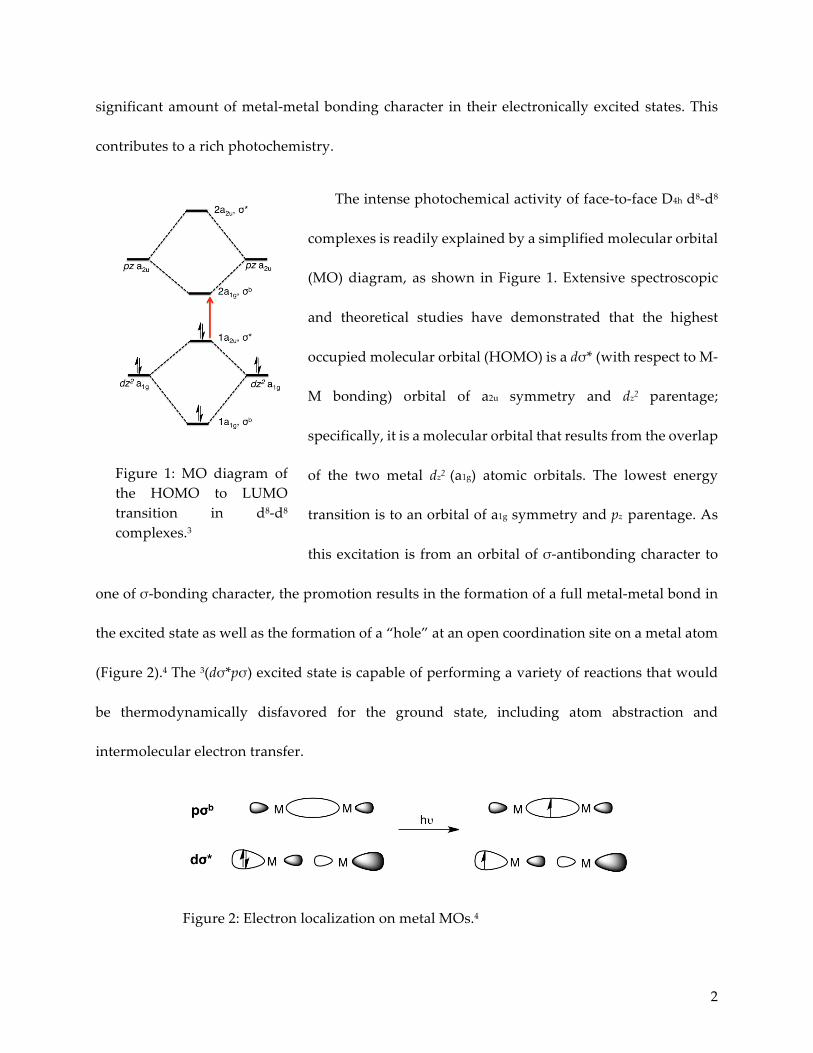
significant amount of metal-metal bonding character in their electronically excited states. This
contributes to a rich photochemistry.
The intense photochemical activity of face-to-face D4h d8-d8
complexes is readily explained by a simplified molecular orbital
(MO) diagram, as shown in Figure 1. Extensive spectroscopic
and theoretical studies have demonstrated that the highest
occupied molecular orbital (HOMO) is a dσ* (with respect to M-
M bonding) orbital of a2u symmetry and dz2 parentage;
specifically, it is a molecular orbital that results from the overlap
of the two metal dz2 (a1g) atomic orbitals. The lowest energy
transition is to an orbital of a1g symmetry and pz parentage. As
this excitation is from an orbital of σ-antibonding character to
one of σ-bonding character, the promotion results in the formation of a full metal-metal bond in
the excited state as well as the formation of a “hole” at an open coordination site on a metal atom
(Figure 2).4 The 3(dσ*pσ) excited state is capable of performing a variety of reactions that would
be thermodynamically disfavored for the ground state, including atom abstraction and
intermolecular electron transfer.
Figure 2: Electron localization on metal MOs.4
Figure 1: MO diagram of the HOMO to LUMO transition in d8-d8 complexes.3

3
The study of d8-d8 dimeric compounds has long been a theme in the Gray group. In 1976,
researchers in the Gray group first synthesized a dimeric RhI complex ligated by four 1,3-
diisocyanopropane (“bridge”) moieties. This compound, when irradiated at 546 nm in an
aqueous solution of HCl, was found to produce hydrogen gas with concomitant oxidation of the
complex to form [Rh2(bridge)4Cl2]2+. In 1990, Fox and coworkers studied the kinetics of
photoinduced electron transfer d8-d8 Ir2 phosphonite complexes and demonstrated the existence
of an inverted free-energy dependence of electron transfer kinetics at high driving forces. This
was one of the first examples of a Marcus “inverted region” in chemical kinetics.5
1.3 Remarkable properties of pyrophosphito-bridged diplatinum(II) compounds
One compound that has garnered particular attention is tetrakis(µ-
pyrophosphito) diplatinate(II)4-, also known as 4- due to its bridging
P-O-P moieties. The compound consists of two d8 square planar ML4
fragments supported by pyrophosphito bridges. The two halves are
eclipsed, giving rise to a lantern-like complex with D4h symmetry
(Figure 3). In the ground state, the Pt-Pt distance is 2.93 Å; while
generally this distance is too long to be considered a bond and the molecular orbital (MO)
diagram indicates a formal bond order of zero, resonance Raman studies as well as recent
theoretical work show that there is indeed some degree of bonding in the ground state due to
favorable mixing of the (n)dz2 and (n+1)pz orbitals.8,9
1.3.1 Photophysical properties
Figure 3: Structure of Pt(pop)4- 6
4
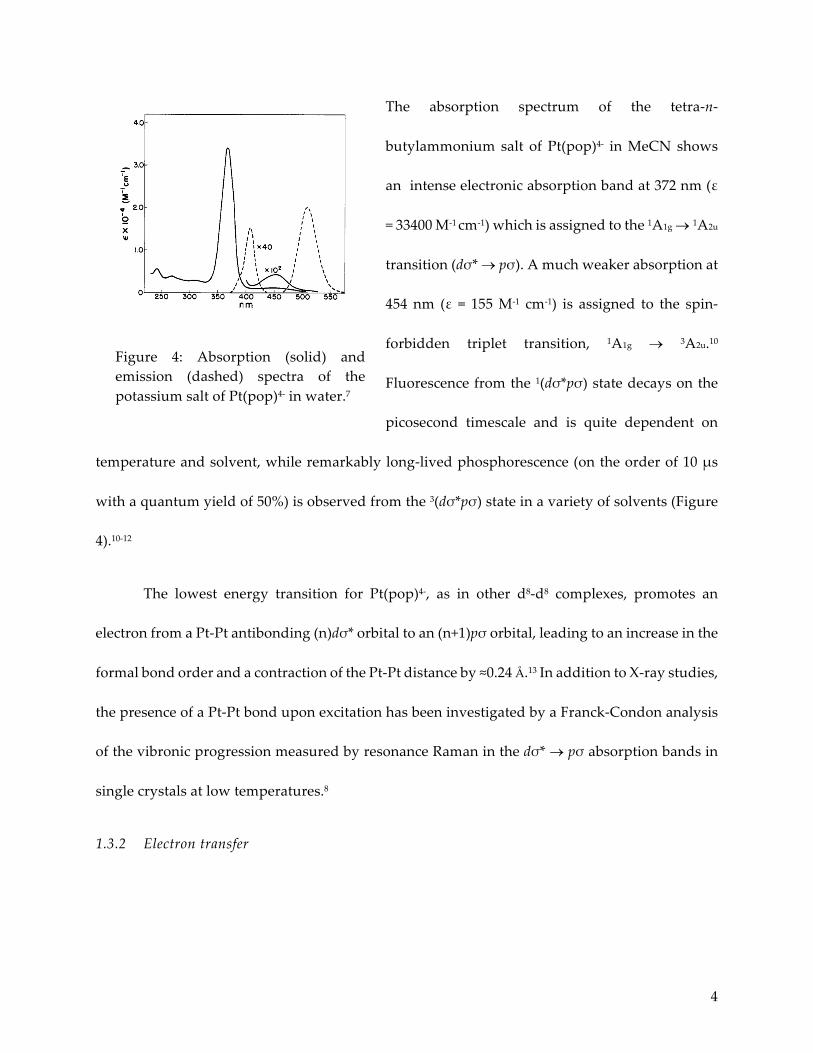
The absorption spectrum of the tetra-n-
butylammonium salt of Pt(pop)4- in MeCN shows
an intense electronic absorption band at 372 nm (ε
= 33400 M-1 cm-1) which is assigned to the 1A1g ® 1A2u
transition (dσ* ® pσ). A much weaker absorption at
454 nm (ε = 155 M-1 cm-1) is assigned to the spin-
forbidden triplet transition, 1A1g ® 3A2u.10
Fluorescence from the 1(dσ*pσ) state decays on the
picosecond timescale and is quite dependent on
temperature and solvent, while remarkably long-lived phosphorescence (on the order of 10 µs
with a quantum yield of 50%) is observed from the 3(dσ*pσ) state in a variety of solvents (Figure
4).10-12
The lowest energy transition for Pt(pop)4-, as in other d8-d8 complexes, promotes an
electron from a Pt-Pt antibonding (n)dσ* orbital to an (n+1)pσ orbital, leading to an increase in the
formal bond order and a contraction of the Pt-Pt distance by ≈0.24 Å.13 In addition to X-ray studies,
the presence of a Pt-Pt bond upon excitation has been investigated by a Franck-Condon analysis
of the vibronic progression measured by resonance Raman in the dσ* ® pσ absorption bands in
single crystals at low temperatures.8
1.3.2 Electron transfer
Figure 4: Absorption (solid) and emission (dashed) spectra of the potassium salt of Pt(pop)4- in water.7
5
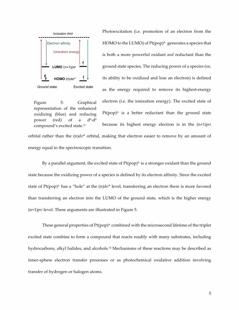
Photoexcitation (i.e. promotion of an electron from the
HOMO to the LUMO) of Pt(pop)4- generates a species that
is both a more powerful oxidant and reductant than the
ground state species. The reducing power of a species (or,
its ability to be oxidized and lose an electron) is defined
as the energy required to remove its highest-energy
electron (i.e. the ionization energy). The excited state of
Pt(pop)4- is a better reductant than the ground state
because its highest energy electron is in the (n+1)pσ
orbital rather than the (n)dσ* orbital, making that electron easier to remove by an amount of
energy equal to the spectroscopic transition.
By a parallel argument, the excited state of Pt(pop)4- is a stronger oxidant than the ground
state because the oxidizing power of a species is defined by its electron affinity. Since the excited
state of Pt(pop)4- has a “hole” at the (n)dσ* level, transferring an electron there is more favored
than transferring an electron into the LUMO of the ground state, which is the higher energy
(n+1)pσ level. These arguments are illustrated in Figure 5.
These general properties of Pt(pop)4- combined with the microsecond lifetime of the triplet
excited state combine to form a compound that reacts readily with many substrates, including
hydrocarbons, alkyl halides, and alcohols.14 Mechanisms of these reactions may be described as
inner-sphere electron transfer processes or as photochemical oxidative addition involving
transfer of hydrogen or halogen atoms.
Figure 5: Graphical representation of the enhanced oxidizing (blue) and reducing power (red) of a d8-d8
compound’s excited state.11
6
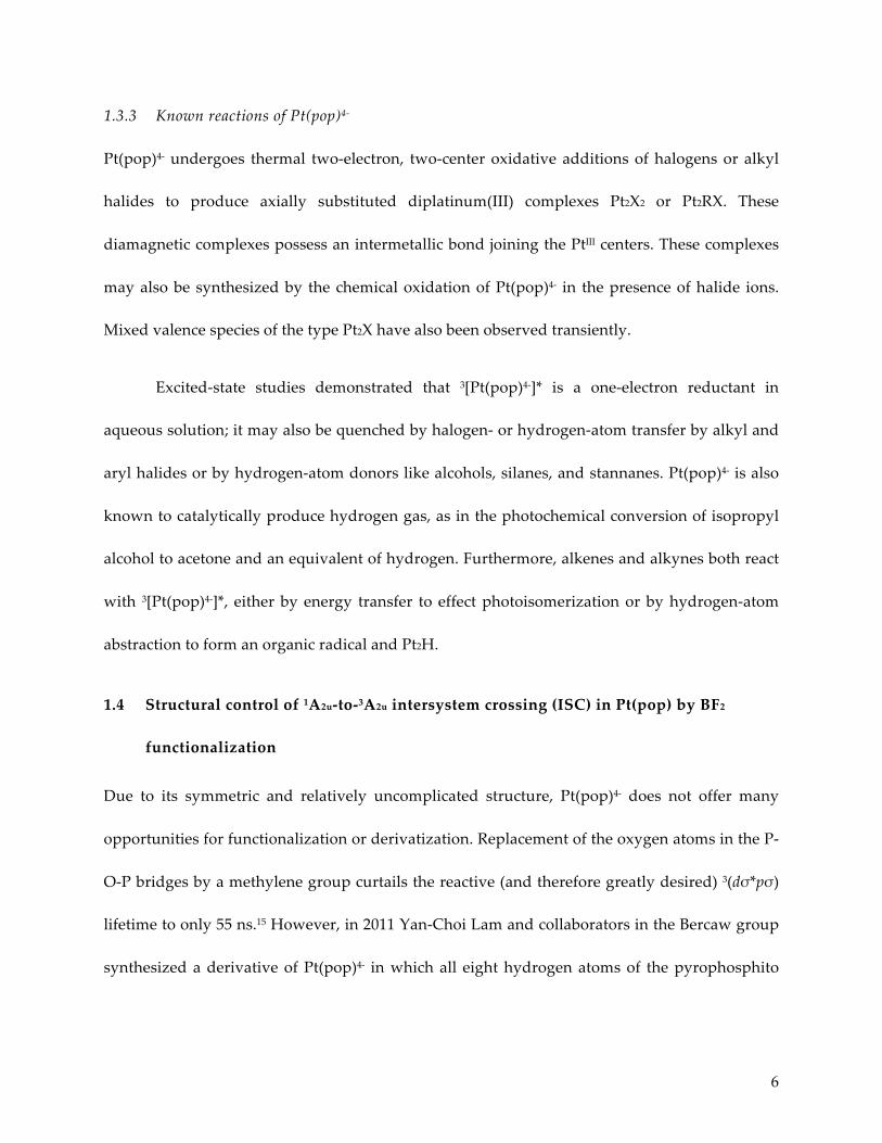
1.3.3 Known reactions of Pt(pop)4-
Pt(pop)4- undergoes thermal two-electron, two-center oxidative additions of halogens or alkyl
halides to produce axially substituted diplatinum(III) complexes Pt2X2 or Pt2RX. These
diamagnetic complexes possess an intermetallic bond joining the PtIII centers. These complexes
may also be synthesized by the chemical oxidation of Pt(pop)4- in the presence of halide ions.
Mixed valence species of the type Pt2X have also been observed transiently.
Excited-state studies demonstrated that 3[Pt(pop)4-]* is a one-electron reductant in
aqueous solution; it may also be quenched by halogen- or hydrogen-atom transfer by alkyl and
aryl halides or by hydrogen-atom donors like alcohols, silanes, and stannanes. Pt(pop)4- is also
known to catalytically produce hydrogen gas, as in the photochemical conversion of isopropyl
alcohol to acetone and an equivalent of hydrogen. Furthermore, alkenes and alkynes both react
with 3[Pt(pop)4-]*, either by energy transfer to effect photoisomerization or by hydrogen-atom
abstraction to form an organic radical and Pt2H.
1.4 Structural control of 1A2u-to-3A2u intersystem crossing (ISC) in Pt(pop) by BF2
functionalization
Due to its symmetric and relatively uncomplicated structure, Pt(pop)4- does not offer many
opportunities for functionalization or derivatization. Replacement of the oxygen atoms in the P-
O-P bridges by a methylene group curtails the reactive (and therefore greatly desired) 3(dσ*pσ)
lifetime to only 55 ns.15 However, in 2011 Yan-Choi Lam and collaborators in the Bercaw group
synthesized a derivative of Pt(pop)4- in which all eight hydrogen atoms of the pyrophosphito

7
groups are replaced with electron-withdrawing BF2 groups, each of which links the oxygen atoms
of two different bridges to form a cage-like structure (Figure 6).14
Figure 6: Synthesis of Pt(pop-BF2)4-
This compound, per(difluoroboro)tetrakis(µ-pyrophosphito)diplatinate(II)4-, will be referred
to as Pt(pop-BF2)4- for the remainder of this work. The electron-withdrawing nature of the BF2
groups has the effect of removing electron density from the phosphorus atoms that are directly
ligated to the PtII centers. This stabilizes the dπ levels in Pt(pop-BF2)4- compared to Pt(pop)4-,
making it a stronger oxidant than the parent compound.
1.5 Photophysical implications of BF2 functionalization
The “perfluoroboration” of Pt(pop) has dramatic effects on its photophysical properties. Table 1
compares the absorption and emission properties of Pt(pop)4- and Pt(pop-BF2)4-.14
Table1:ComparisonofPt(pop)4-andPt(pop-BF2)4-
Pt(pop-BF2)4- Pt(pop)4- Assignment

8
Absorption,nm(ε,M-1cm-1)
233(7880) 246(3770) LMMCT
260(3180) 285(2550) LMMCT
291(2110) 315(1640) LMMCT
365(37500) 372(33400) 1(dσ*àpσ)1A1gà1A2u
454(140) 454(155) 3(dσ*àpσ)1A1gà3A2u
Emission,nm(Lifetimeat21°C)
393(1.6ns) 398(~8ps) 1(pσàdσ*)1A2uà1A1g
512(8.4µs) 511(9.4µs) 3(pσàdσ*)3A2uà1A1g
EmissionStokesShift,cm-1
1760 2230 Fluorescence
2460 2500 Phosphorescence
EaforISC(cm-1)
2230 1190 1A2u-3EuS-Ocoupling
The metal-centered absorption features (the ds*® pσ transitions) of Pt(pop-BF2)4- are similar to
those of Pt(pop)4-; shifts of only about five hundred wavenumbers are observed. This is expected,
as the BF2 functionalization should not affect the d ® p absorption features; the effect of the BF2
groups is instead to stabilize the metal-centered orbitals as a whole. The most intense band at 365
nm (27397 cm-1) results from the dσ* ® pσ (1A1g ® 1A2u) transition; the same transition in Pt(pop)4-
occurs at 372 nm (26881 cm-1). The much more weakly absorbing spin forbidden singlet-to-triplet
9
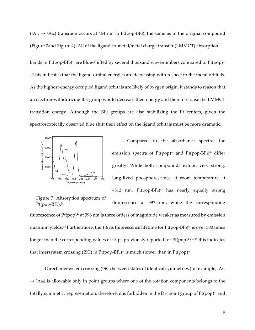
(1A1g ® 3A2u) transition occurs at 454 nm in Pt(pop-BF2), the same as in the original compound
(Figure 7and Figure 4). All of the ligand-to-metal/metal charge transfer (LMMCT) absorption
bands in Pt(pop-BF2)4- are blue-shifted by several thousand wavenumbers compared to Pt(pop)4-
. This indicates that the ligand orbital energies are decreasing with respect to the metal orbitals.
As the highest-energy occupied ligand orbitals are likely of oxygen origin, it stands to reason that
an electron-withdrawing BF2 group would decrease their energy and therefore raise the LMMCT
transition energy. Although the BF2 groups are also stabilizing the Pt centers, given the
spectroscopically observed blue shift their effect on the ligand orbitals must be more dramatic.
Compared to the absorbance spectra, the
emission spectra of Pt(pop)4- and Pt(pop-BF2)4- differ
greatly. While both compounds exhibit very strong,
long-lived phosphorescence at room temperature at
~512 nm, Pt(pop-BF2)4- has nearly equally strong
fluorescence at 393 nm, while the corresponding
fluorescence of Pt(pop)4- at 398 nm is three orders of magnitude weaker as measured by emission
quantum yields.14 Furthermore, the 1.6 ns fluorescence lifetime for Pt(pop-BF2)4- is over 500 times
longer than the corresponding values of ~3 ps previously reported for Pt(pop)4-;16-18 this indicates
that intersystem crossing (ISC) in Pt(pop-BF2)4- is much slower than in Pt(pop)4-.
Direct intersystem crossing (ISC) between states of identical symmetries (for example, 1A2u
® 3A2u) is allowable only in point groups where one of the rotation components belongs to the
totally symmetric representation; therefore, it is forbidden in the D4h point group of Pt(pop)4- and
Figure 7: Absorption spectrum of Pt(pop-BF2).14

10
Pt(pop-BF2)4-. However, ISC may become partially allowed via spin-orbit coupling with higher
triplet states. In Pt(pop)4- and Pt(pop-BF2)4-, this higher triplet state of interest is likely the 3Eu of
LMMCT origin. By undergoing symmetry-allowed spin-orbit coupling with the 3Eu state, the 1A2u
state is able to cross to the 3A2u state, thus leading to the long-lived phosphorescence observed in
both the Pt24- complexes.
The 500-fold less rapid ISC in Pt(pop-BF2)4- versus Pt(pop)4- is attributable to the fact that
ISC results from spin-orbit coupling to an LMMCT state. The BF2 groups lower the energy of the
ligand states, as evidenced by the higher-energy LMMCT bands in the absorption spectra. A
higher energy 3Eu state makes spin-orbit coupling with the 1A2u state less favorable, thereby
slowing the rate of ISC in Pt(pop-BF2)4-. Furthermore, solvent vibrations are quite important for
acting as energy-accepting modes during ISC, as evidenced by the strong solvent dependence of
Pt(pop)4- decay kinetics.17 Given that BF2 groups are both bulkier than the O–H���O– groups and
that they form a rigid covalent cage rather than a more flexible hydrogen bonded one, one would
expect that solvent interactions would be diminished. By that reasoning, the ability of the solvent
to provide vibrational coupling between the singlet and triplet states is reduced for Pt(pop-BF2)4.
The dramatic reduction in the rate of intersystem crossing and the concomitant increase in ISC
activation energy, from 1190 cm-1 for Pt(pop)4- to 2230 cm-1 for Pt(pop-BF2)4-, is the reason for the
much longer lived singlet in the perfluoroborated compound (1.6 ns vs 8 ps).
1.6 Electrochemical implications of BF2 functionalization

11
As discussed in section 1.4, the BF2 groups were
predicted to make Pt(pop-BF2)4- a stronger
oxidant. Recent research published by myself
and Bryan Hunter et al. places the potential of the
reversible Pt(pop-BF2)4-/5- couple at -1.68 V vs
Fc+/Fc while also predicting the existence of an
even more reduced compound, Pt(pop-BF2)6-,
due to a second irreversible reduction wave at -
2.46 V.19 As expected, the single electron
reduction potential for Pt(pop-BF2)4- lies at a more positive potential than that of Pt(pop)4-. A
Latimer diagram illustrating the electrochemical differences between the two compounds is
presented in Figure 9. The excited state reduction potential for 3[Pt(pop-BF2)4-]* is estimated based
on spectroscopic data to be approximately 1.0 V, which makes it comparable in oxidative strength
to compounds like [NO]+ (Eº’ = 1.0 V vs Fc/Fc+ in CH2Cl2) and [Ru(phen)3]3+ (Eº’ ≈ 0.87 V vs Fc/Fc+
in CH3CN).20 Meanwhile, 1[Pt(pop-BF2)4-]* is expected to have even more oxidizing power, as the
spectroscopic difference between the absorption peaks for the triplet and the singlet is ≈5000 cm-
1, which corresponds to a 620 mV more positive potential. Given the short lifetime of the singlet
state, it is improbable that this oxidizing power could be utilized in a diffusional solution setting;
however, the possibilities for direct charge- or energy-transfer to substrates are substantial.
i Historic values for Pt(pop)4- were reported by Harvey in acetonitrile with respect to NHE; potentials were converted to a ferrocene reference by adding 0.64 V.
Figure 9: Latimer diagram for Pt(pop)4- and Pt(pop-BF2)4-. Reduction potentials (all reported versus Fc+/Fc) i for Pt(pop) are written in black;11 reduction potentials for Pt(pop-BF2) are written in green italics.19

12
1.7 Applications
The oxidative strength of [Pt(pop-BF2)4-]* and its steric bulk, combined with the fact that the
production of the excited state is phototriggered, make it an attractive candidate for probing
reactivity via transient absorption (TA) spectroscopy. As previously mentioned, canonical
Pt(pop)4- is capable of performing a variety of organic transformations on its own due to the
rotational flexibility of the terminal hydroxyl groups. This flexibility leaves the metal centers
unblocked, and these open axial coordination sites on each Pt atom allow “docking” of various
substrates with subsequent atom abstraction. The much more hindered and rigidly covalent BF2
cage precludes this type of reactivity in Pt(pop-BF2)4-. Unpublished results in the Gray Group
obtained by Yan-Choi Lam indicate that Pt(pop-BF2)4- possesses very little, if any, of the inherent
reactivity of Pt(pop)4- discussed in 1.3.3. For example, Pt(pop)4- reacts rapidly with iodomethane
to form the oxidative addition product, but Pt(pop-BF2)4- is wholly unreactive toward such
powerful electrophiles.21 However, considering the case where only electron transfer is desired
from Pt(pop-BF2)4- to trigger reactivity in a different molecule, this lack of reactivity is actually
quite a boon. Given its relative inertness, Pt(pop-BF2)4- is hoped to act as an outer sphere electron
transfer agent only, with little or no inherent reactivity of its own. Meanwhile, the reduced (5-)
and superreduced (6-) states are expected to be much more reactive than the parent compound
and may act directly as catalytic agents. Initial studies in these areas will be discussed.
13
REFERENCES
(1) Atoji, M.; Richardson, J. W.; Rundle, R. E. J. Am. Chem. Soc. 1957, 79, 3017. (2) Yam, V. W.-W.; Au, V. K.-M.; Leung, S. Y.-L. Chem. Rev. 2015, 115, 7589. (3) Mann, K. R.; Gordon, J. G.; Gray, H. B. J. Am. Chem. Soc. 1975, 97, 3553. (4) Smith, D. C.; Gray, H. B. Coord. Chem. Rev. 1990, 100, 169. (5) Fox, L. S.; Kozik, M.; Winkler, J. R.; Gray, H. B. Science 1990, 247, 1069. (6) Pan, Q.-J.; Fu, H.-G.; Yu, H.-T.; Zhang, H.-X. Inorg. Chem. 2006, 45, 8729. (7) Che, C. M.; Butler, L. G.; Gray, H. B. J. Am. Chem. Soc. 1981, 103, 7796. (8) Che, C. M.; Butler, L. G.; Gray, H. B.; Crooks, R. M.; Woodruff, W. H. J. Am. Chem.
Soc. 1983, 105, 5492. (9) Bercaw, J. E.; Durrell, A. C.; Gray, H. B.; Green, J. C.; Hazari, N.; Labinger, J. A.;
Winkler, J. R. Inorg. Chem. 2010, 49, 1801. (10) Stiegman, A. E.; Rice, S. F.; Gray, H. B.; Miskowski, V. M. Inorg. Chem. 1987, 26,
1112. (11) Harvey, E. L. Dissertation (Ph.D.), California Institute of Technology, 1990. (12) Heuer, W. B.; Totten, M. D.; Rodman, G. S.; Hebert, E. J.; Tracy, H. J.; Nagle, J. K.
J. Am. Chem. Soc. 1984, 106, 1163. (13) Christensen, M.; Haldrup, K.; Bechgaard, K.; Feidenhans'l, R.; Kong, Q.;
Cammarata, M.; Russo, M. L.; Wulff, M.; Harrit, N.; Nielsen, M. M. J. Am. Chem. Soc. 2008, 131, 502.
(14) Durrell, A. C.; Keller, G. E.; Lam, Y.-C.; Sykora, J.; Vlček, A.; Gray, H. B. J. Am. Chem. Soc. 2012, 134, 14201.
(15) King, C.; Auerbach, R. A.; Fronczek, F. R.; Roundhill, D. M. J. Am. Chem. Soc. 1986, 108, 5626.
(16) van der Veen, R. M.; Cannizzo, A.; van Mourik, F.; Vlček, A.; Chergui, M. J. Am. Chem. Soc. 2010, 133, 305.
(17) Milder, S. J.; Brunschwig, B. S. J. Phys. Chem. 1992, 96, 2189. (18) Vlček, A. 2016. (19) Darnton, T. V.; Hunter, B. M.; Hill, M. G.; Záliš, S.; Vlček, A.; Gray, H. B. J. Am.
Chem. Soc. 2016, 138, 5699. (20) Connelly, N. G.; Geiger, W. E. Chem. Rev. 1996, 96, 877. (21) Lam, Y.-C.; Darnton, T. Unpublished results.
14
CHAPTER 2: SYNTHESIS AND CHARACTERIZATION OF Pt(POP-BF2)4-
As discussed in Chapter 1, Pt(pop)4- participates in and facilitates a wide array of reactions. In its
excited state, [Pt(pop)4-]* is able to abstract hydrogen atoms from a variety of substrates including
stannanes, silanes, alcohols, and hydrocarbons. It also reacts readily with alkyl and aryl halides
(R or RX) to form the axially substituted PtIII-PtIII oxidative addition product (i.e. [Pt(pop)-RX]4- or
[Pt(pop)-X2]4-) and, in the case of dihalide, the corresponding organic radical coupling product R2.
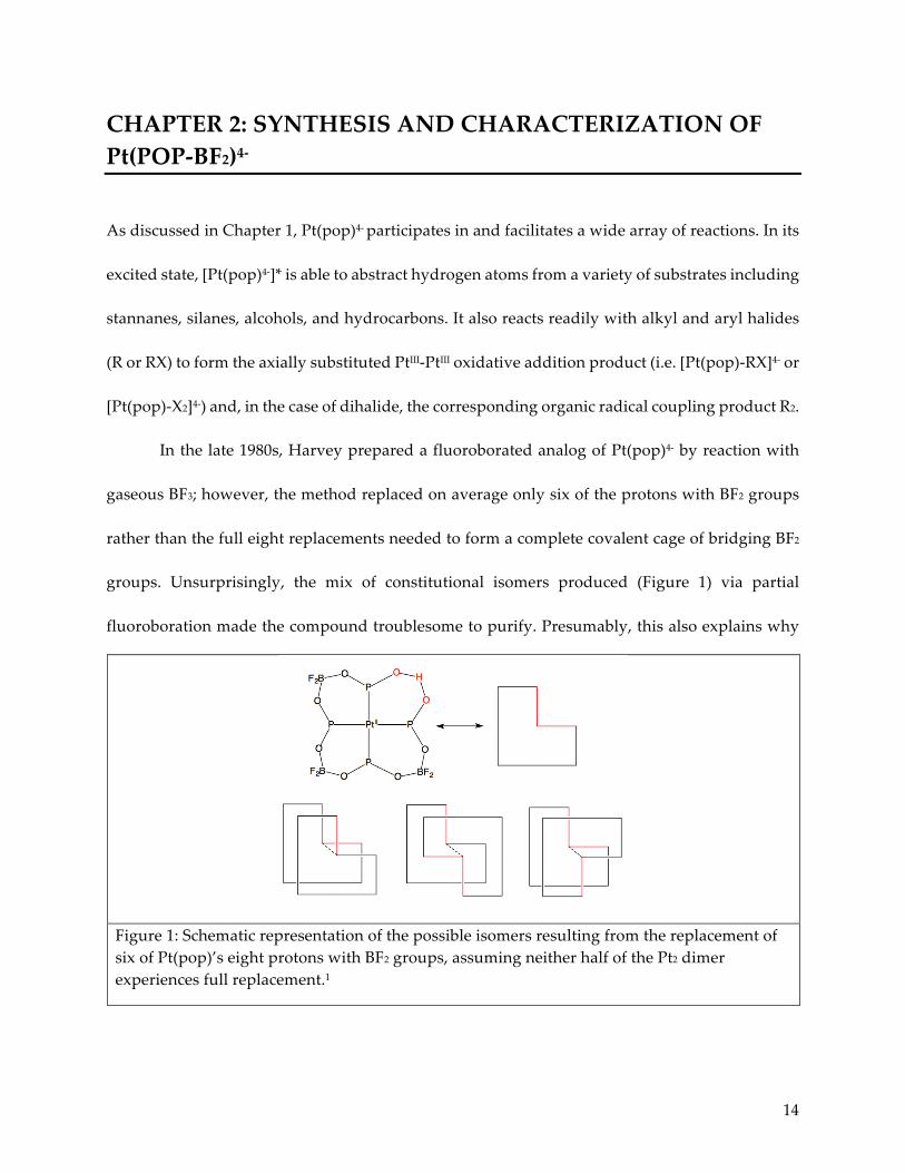
In the late 1980s, Harvey prepared a fluoroborated analog of Pt(pop)4- by reaction with
gaseous BF3; however, the method replaced on average only six of the protons with BF2 groups
rather than the full eight replacements needed to form a complete covalent cage of bridging BF2
groups. Unsurprisingly, the mix of constitutional isomers produced (Figure 1) via partial
fluoroboration made the compound troublesome to purify. Presumably, this also explains why
Figure 1: Schematic representation of the possible isomers resulting from the replacement of six of Pt(pop)’s eight protons with BF2 groups, assuming neither half of the Pt2 dimer experiences full replacement.1

15
Harvey was not able at the time to rigorously determine the compound’s properties, particularly
with respect to NMR signatures.1
In 2011, Yan-Choi Lam and collaborators in the lab of John Bercaw developed a more
robust and reliable synthetic method for producing Pt(pop-BF2)4- by stirring Pt(pop)4- in neat
boron trifluoride diethyletherate (BF3•Et2O) for several days.2 Initial experiments performed by
Durrell, Lam, and Keller indicated that Pt(pop-BF2)4-, as predicted by Harvey, possessed unique
luminescence properties that clearly differentiated it from its parent, Pt(pop)4-.2 In late 2012,
intrigued by this relatively new and unexplored compound, I decided to devote my doctoral
research to its study.
2.1 Synthetic developments
Before embarking on more complex analytical studies of Pt(pop-BF2)4-‘s luminescence and
reactivity, I first endeavored to corroborate the basic synthetic and luminescence results reported
by Durrell and coworkers. As a result, I further developed Lam’s synthesis of Pt(pop-BF2)4- by
improving the glassware setup and work-up techniques to decrease the possibility of exposure
to BF3•Et2O or its hydration product, hydrofluoric acid (see section 2.4.6).
During this process, the tetraphenylphosphonium (Ph4P+) salt of Pt(pop-BF2)4- was
crystallized and characterized via X-ray diffraction for the first time (Figure 2). Prior to this point,
only the tetrabutylammonium ((n-Bu)4N+) salt had been reported in the literature, although the
tetraphenylarsonium (Ph4As+) salt had also been accessed by Lam.2-4 In [Ph4P]4[Pt(pop-BF2)], the
distance between the largest electron density maxima is 2.85 Å, which corresponds to the Pt-Pt
distance. However, the compound crystallizes in the monoclinic space group P21/n with only half

16
of the molecule and two tetraphenylphosphonium
cations in the asymmetric unit. Attempts to refine the
density maxima as a second platinum position were
unsuccessful; this could account for the slight
discrepancy between this 2.85 Å distance and Lam’s
previously reported value of 2.89 Å for the
tetraphenylarsonium salt of Pt(pop-BF2)4-.4 Both the Pt-Pt
distance values for salts of Pt(pop-BF2)4- are significantly
smaller than the value of 2.93 Å reported for K4Pt(pop);
this could be attributed to the overall contraction of the Pt-Pt unit due to the rigidity of the BF2
covalent “cage.”4,5 X-ray data are tabulated in Table 1 through Table 5 in section 2.6.
2.2 Basic luminescence properties
With the goal of duplicating the values for 𝐸", 𝑘% and 𝑘& obtained by Durrell and coworkers,
solutions of Pt(pop-BF2)4- in acetonitrile were analyzed via both time-resolved and steady-state
techniques to obtain values for fluorescence lifetime and quantum yield. With values for
fluorescence lifetime and quantum yield in hand, values for 𝐸", 𝑘%, and 𝑘& can be calculated.
These new data were compared directly to the values published in 2012.
Theoretical basis
In their 1992 publication probing the luminescence lifetimes of Pt(pop)4-, Milder and
Brunschwig presented an elegant series of experiments and equations for combining time-
resolved and steady-state data taken at various temperatures to determine the activation energy
of intersystem crossing between the singlet and triplet excited states, as well as the rates of
Figure 2: Crystal structure of [Ph4P]4[Pt(pop-BF2)].

17
radiative and nonradiative decay from the singlet state. These equations were applied to
Pt(pop-BF2)4- by Durrell and coworkers.
In Pt(pop-BF2)4-, analogously to Pt(pop)4-, an electron in the singlet excited state has
several pathways available by which to return to the ground state. It may nonradiatively decay
(that is, decay without emitting a photon) or radiatively decay by emitting a photon
(fluorescence). Nonradiative decay may occur either by intersystem crossing to the triplet state
or by nonemissive decay to the ground state (for example, due to energy loss from solvent
interactions). The rate of nonemissive decay to the ground state is represented by the rate
constant 𝑘' while the rate of intersystem crossing is represented by the rate constant 𝑘()* ; the
rate of radiative decay is denoted by 𝑘%. Therefore, the total amount of nonradiative decay may
be represented by the sum of 𝑘' and 𝑘()* . As proposed by Milder and Brunschwig for Pt(pop)4-,
𝑘()* for Pt(pop-BF2)4- is presumed to follow Arrhenius-like behavior.
𝑘+% = 𝑘' + 𝑘()* = 𝑘' + 𝑘& +𝐴𝑘/𝑇
𝑒234567 ( 1 )
Meanwhile, the fluorescence lifetime (𝜏9:) is inversely proportional to the rates of the decay
paths out of the excited state:
1𝜏9:
= 𝑘% + 𝑘+% = 𝑘% + 𝑘' + 𝑘& +𝐴𝑘/𝑇
𝑒234567 ( 2 )
The lifetime 𝜏9: may be extracted from a luminescence-decay plot. By observing 𝜏9: at various
temperatures, the following relation derived from equation ( 2 ) used with an appropriate fitting
program may be used to find values for the unknowns 𝐴, 𝐸", and 𝑘% + 𝑘' + 𝑘&.
18
𝑦 =
1𝜏9:
𝑦 = 𝛼 +
𝛽 𝑥0.695
𝑒2EF&.GHI ( 3 )
𝑥 =1𝑇
in which
𝛼 = 𝑘% + 𝑘' + 𝑘& ≈ 𝑘% + 𝑘&
𝛽 = 𝐴
𝛾 = 𝐸"
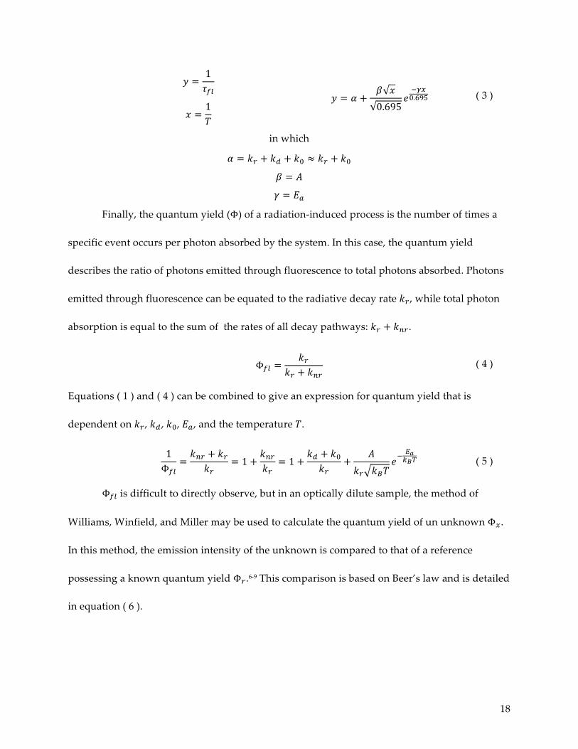
Finally, the quantum yield (Φ) of a radiation-induced process is the number of times a
specific event occurs per photon absorbed by the system. In this case, the quantum yield
describes the ratio of photons emitted through fluorescence to total photons absorbed. Photons
emitted through fluorescence can be equated to the radiative decay rate 𝑘%, while total photon
absorption is equal to the sum of the rates of all decay pathways: 𝑘% + 𝑘+%.
Φ9: =𝑘%
𝑘% + 𝑘+% ( 4 )
Equations ( 1 ) and ( 4 ) can be combined to give an expression for quantum yield that is
dependent on 𝑘%, 𝑘', 𝑘&, 𝐸", and the temperature 𝑇.
1Φ9:
=𝑘+% + 𝑘%
𝑘%= 1 +
𝑘+%𝑘%
= 1 +𝑘' + 𝑘&𝑘%
+𝐴
𝑘% 𝑘/𝑇𝑒2
34567 ( 5 )
Φ9: is difficult to directly observe, but in an optically dilute sample, the method of
Williams, Winfield, and Miller may be used to calculate the quantum yield of un unknown ΦF.
In this method, the emission intensity of the unknown is compared to that of a reference
possessing a known quantum yield Φ%.6-9 This comparison is based on Beer’s law and is detailed
in equation ( 6 ).

19
ΦF = Φ%𝐴% 𝜆%𝐴F 𝜆F
𝐼 𝜆%𝐼 𝜆F
𝑛FP
𝑛%P𝐷F𝐷%
( 6 )
in which
ΦF = 𝑞𝑢𝑎𝑛𝑡𝑢𝑚𝑦𝑖𝑒𝑙𝑑𝑜𝑓𝑢𝑛𝑘𝑛𝑜𝑤𝑛
Φ% =quantumyieldofreferencecompound(tabulated)
𝐴 𝜆 = 𝑎𝑏𝑠𝑜𝑟𝑏𝑎𝑛𝑐𝑒𝑝𝑒𝑟𝑐𝑚𝑜𝑓𝑠𝑜𝑙𝑢𝑡𝑖𝑜𝑛𝑎𝑡𝑒𝑥𝑐𝑖𝑡𝑎𝑡𝑖𝑜𝑛𝑤𝑎𝑣𝑒𝑙𝑒𝑛𝑔𝑡ℎ𝜆
𝐼 𝜆 = 𝑟𝑒𝑙𝑎𝑡𝑖𝑣𝑒𝑖𝑛𝑡𝑒𝑛𝑠𝑖𝑡𝑦𝑜𝑓𝑒𝑥𝑐𝑖𝑡𝑎𝑡𝑖𝑜𝑛𝑙𝑖𝑔ℎ𝑡𝑎𝑡𝜆
𝑛 = 𝑎𝑣𝑒𝑟𝑎𝑔𝑒𝑟𝑒𝑓𝑟𝑎𝑐𝑡𝑖𝑣𝑒𝑖𝑛𝑑𝑒𝑥𝑜𝑓𝑠𝑜𝑙𝑣𝑒𝑛𝑡
𝐷 = 𝑖𝑛𝑡𝑒𝑔𝑟𝑎𝑡𝑒𝑑𝑎𝑟𝑒𝑎𝑢𝑛𝑑𝑒𝑟𝑒𝑚𝑖𝑠𝑠𝑖𝑜𝑛𝑠𝑝𝑒𝑐𝑡𝑟𝑢𝑚
With temperature-dependent quantum yield data in hand, the following function extracted
from equation ( 5 ) used with an appropriate fitting program may be used to extract relations
for 𝑘&, 𝑘%, 𝐴,and 𝐸".
𝑦 =
1Φ9:
𝑦 = 1 + 𝑎 +
𝑏 𝑥0.695
𝑒2yF&.GHI ( 7 )
𝑥 =1𝑇
in which
𝑎 =𝑘' + 𝑘&𝑘%
≈𝑘&𝑘%
𝑏 =𝐴𝑘%
𝑐 = 𝐸"
The values calculated for the fitting parameters 𝑎, 𝑏, 𝑐, 𝛼, 𝛽,and 𝛾 using equations ( 3 ) and ( 7 )
can then be combined to obtain values for the unknowns 𝑘%, 𝑘&, 𝐴, and 𝐸":
𝑘% =𝛽𝑏
𝑘& =𝛽𝑎𝑏
𝐴 = 𝛽
𝐸" = 𝛾 = 𝑐
( 8 )
20
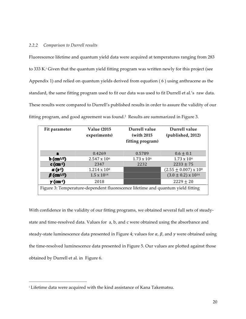
Comparison to Durrell results
Fluorescence lifetime and quantum yield data were acquired at temperatures ranging from 283
to 333 K.i Given that the quantum yield fitting program was written newly for this project (see
Appendix 1) and relied on quantum yields derived from equation ( 6 ) using anthracene as the
standard, the same fitting program used to fit our data was used to fit Durrell et al.’s raw data.
These results were compared to Durrell’s published results in order to assure the validity of our
fitting program, and good agreement was found.2 Results are summarized in Figure 3.
Fit parameter Value (2015 experiments)
Durrell value (with 2015
fitting program)
Durrell value (published, 2012)
a 0.4269 0.5789 0.6±0.1b(cm1/2) 2.547x10⁶ 1.73x10⁶ 1.73x10⁶c(cm-1) 2347 2232 2233±75𝛼(s-1) 1.214x10⁸ (2.55±0.007)x108
𝛽(cm1/2) 1.5x10¹⁴ (3.0±0.2)x1014𝛾(cm-1) 2018 2229±20
Figure 3: Temperature-dependent fluorescence lifetime and quantum yield fitting
With confidence in the validity of our fitting programs, we obtained several full sets of steady-
state and time-resolved data. Values for a, b, and c were obtained using the absorbance and
steady-state luminescence data presented in Figure 4; values for 𝛼, 𝛽, and 𝛾 were obtained using
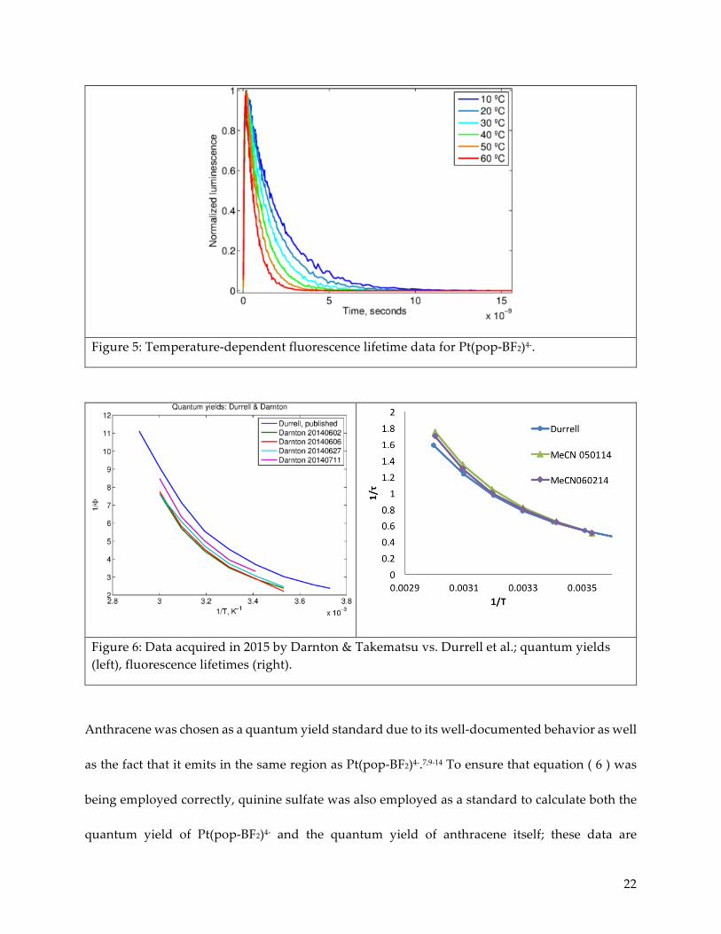
the time-resolved luminescence data presented in Figure 5. Our values are plotted against those
obtained by Durrell et al. in Figure 6.
i Lifetime data were acquired with the kind assistance of Kana Takematsu.

21
Figure 4: Absorbance data for Pt(pop-BF2)4- and anthracene quantum yield standard (top) with steady-state luminescence data for Pt(pop-BF2)4- (middle) and anthracene (bottom).
22
Figure 5: Temperature-dependent fluorescence lifetime data for Pt(pop-BF2)4-.
Figure 6: Data acquired in 2015 by Darnton & Takematsu vs. Durrell et al.; quantum yields (left), fluorescence lifetimes (right).
Anthracene was chosen as a quantum yield standard due to its well-documented behavior as well
as the fact that it emits in the same region as Pt(pop-BF2)4-.7,9-14 To ensure that equation ( 6 ) was
being employed correctly, quinine sulfate was also employed as a standard to calculate both the
quantum yield of Pt(pop-BF2)4- and the quantum yield of anthracene itself; these data are

23
presented in Figure 7 and summarized in Figure 8. Based on these results, it was concluded that
anthracene was an appropriate standard for calculating the quantum yield of Pt(pop-BF2)4-
emission.
Figure 7: Pt(pop-BF2)4-, anthracene, and quinine sulfate absorbance (left) and luminescence (right) spectra.
Reference used 𝛷fl(T=298K)
Pt(pop-BF2)4- Anthracene Anthracene 0.35 n/aQuininesulfate 0.31 0.22
Accepted values: 𝛷flPt(pop-BF2)4-≈0.35;𝛷fl(anthracene)=0.2713
Figure 8: Quantum yield tests
2.3 Pt(pop-BF2)4- luminescence in different solvents
A study published in the early 1990s by Brunchschwig and Milder found that the rate of
nonradiative decay for the singlet excited state in Pt(pop)4- had a strong dependency on solvent,
particularly with regards to solvent polarity and the presence of exchangeable protons. After
significant analysis, they concluded that the vibrations coupling the singlet and triplet state in

24
Pt(pop)4- are solvent modes and/or modes representing the interaction of the solvent with the 1A2u
and 3A2u states of the complex along the Pt-Pt axial coordinate.15
It was expected that the rigidity and steric bulk of Pt(pop-BF2)4-, along with its lack of
exchangeable ligands, would afford more protection from solvents. However, initial results
reported by collaborator Tony Vlček indicated that Pt-Pt vibrational coherence in Pt(pop-BF2)4-
survived intersystem crossing and that the time constants were approximately equal to those
found for Pt(pop)4-. This raised the possibility that the Pt atoms in Pt(pop-BF2)4- were not as well-
shielded as we had previously thought them to be, and were perhaps still exposed to solvent
molecules. With this in mind, experiments were undertaken to quantify the effect of solvent on
Pt(pop-BF2)4- excited state dynamics.
Solvent choice and solvent stability
Unfortunately, Pt(pop-BF2)4- is much less soluble in common solvents than Pt(pop)4-. All previous
experiments involving Pt(pop-BF2)4- were completed in acetonitrile, in which it is quite soluble. It
is insoluble in less polar solvents like diethyl ether, toluene, and tetrahydrofuran, and
decomposes in dichloromethane. While Pt(pop-BF2)4- is soluble in dimethyl sulfoxide and
dimethylformamide, such solvents are exceedingly difficult to keep anhydrous and
uncontaminated due to their extreme polarity, in addition to being costly when purchased in the
requisite high purities.
The greatest effects on the excited state dynamics of Pt(pop)4- were noted by Milder et al.
in methanol and ethanol. As such, samples of ethanol and methanol were purified and dried
according to published protocols.16 Pt(pop-BF2)4- proved to be insoluble in ethanol and only
sparingly soluble in methanol, and it decomposed significantly in both methanol and

25
methanol/acetonitrile mixtures as noted by significant broadening of the characteristic
absorbance maximum at 365 nm. This was followed by a loss of absorption intensity and a slight
blue-shift in wavelength over 24 hours (Figure 9).
Figure 9: Stability of Pt(pop-BF2)4- over 24 hours in acetonitrile, acetonitrile/methanol, and methanol. Absorbance profile is maintained in acetonitrile (purple); immediate peak broadening and loss of intensity over time noted in acetonitrile/methanol (blue) and methanol (red).
This decomposition in methanol is attributed, at least initially, to removal of the BF2 groups by
protonation to reform Pt(pop)4-. This is supported by steady-state fluorescence data obtained in
the same solvents; the emission maxima and the relative sizes of the fluorescence and
phosphorescence peaks in neat methanol and in methanol mixed with acetonitrile are
characteristic of Pt(pop)4-. The control sample measured in acetonitrile maintains the signatures
of Pt(pop-BF2)4-. In Pt(pop-BF2)4- the fluorescence and phosphorescence emission peaks are nearly
equal in intensity; in Pt(pop)4- the phosphorescence peak is ~40x more intense than the
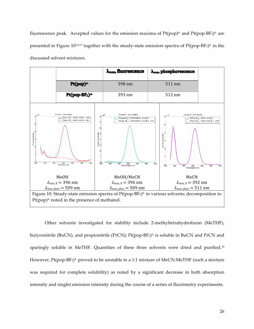
26
fluorescence peak. Accepted values for the emission maxima of Pt(pop)4- and Pt(pop-BF2)4- are
presented in Figure 102,4,17 together with the steady-state emission spectra of Pt(pop-BF2)4- in the
discussed solvent mixtures.
λmax,fluorescence λmax,phosphorescence
Pt(pop)4- 398nm 511nm
Pt(pop-BF2)4- 393nm 512nm
MeOH𝜆max,fl=396nm𝜆max,phos=509nm
MeOH/MeCN𝜆max,fl=396nm𝜆max,phos=509nm
MeCN𝜆max,fl=392nm𝜆max,phos=511nm
Figure 10: Steady-state emission spectra of Pt(pop-BF2)4- in various solvents; decomposition to Pt(pop)4- noted in the presence of methanol.
Other solvents investigated for stability include 2-methyltetrahydrofuran (MeTHF),
butyronitrile (BuCN), and propionitrile (PrCN); Pt(pop-BF2)4- is soluble in BuCN and PrCN and
sparingly soluble in MeTHF. Quantities of these three solvents were dried and purified.16
However, Pt(pop-BF2)4- proved to be unstable in a 1:1 mixture of MeCN:MeTHF (such a mixture
was required for complete solubility) as noted by a significant decrease in both absorption
intensity and singlet emission intensity during the course of a series of fluorimetry experiments.
27
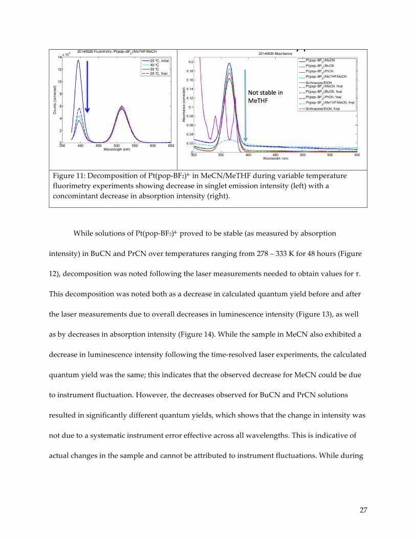
Figure 11: Decomposition of Pt(pop-BF2)4- in MeCN/MeTHF during variable temperature fluorimetry experiments showing decrease in singlet emission intensity (left) with a concomintant decrease in absorption intensity (right).
While solutions of Pt(pop-BF2)4- proved to be stable (as measured by absorption
intensity) in BuCN and PrCN over temperatures ranging from 278 – 333 K for 48 hours (Figure
12), decomposition was noted following the laser measurements needed to obtain values for 𝜏.
This decomposition was noted both as a decrease in calculated quantum yield before and after
the laser measurements due to overall decreases in luminescence intensity (Figure 13), as well
as by decreases in absorption intensity (Figure 14). While the sample in MeCN also exhibited a
decrease in luminescence intensity following the time-resolved laser experiments, the calculated
quantum yield was the same; this indicates that the observed decrease for MeCN could be due
to instrument fluctuation. However, the decreases observed for BuCN and PrCN solutions
resulted in significantly different quantum yields, which shows that the change in intensity was
not due to a systematic instrument error effective across all wavelengths. This is indicative of
actual changes in the sample and cannot be attributed to instrument fluctuations. While during

28
this experiment slightly longer lifetimes were observed in BuCN and PrCN as compared to
MeCN, these data cannot be relied upon due to the sample decomposition.
Figure 12: Absorption profile of Pt(pop-BF2)4- in MeCN (top), BuCN (middle), and PrCN(bottom) at temperatures from 278 – 333 K over 48 hours (day 1 values are solid lines; day 2 values are dashed lines). Insets show the region of maximum absorption.

29
𝛷fl,initial,20ºC𝛷fl,final,20ºC(afterlaser
measurements)
0.33 0.33
0.34 0.21
0.39 0.31
30
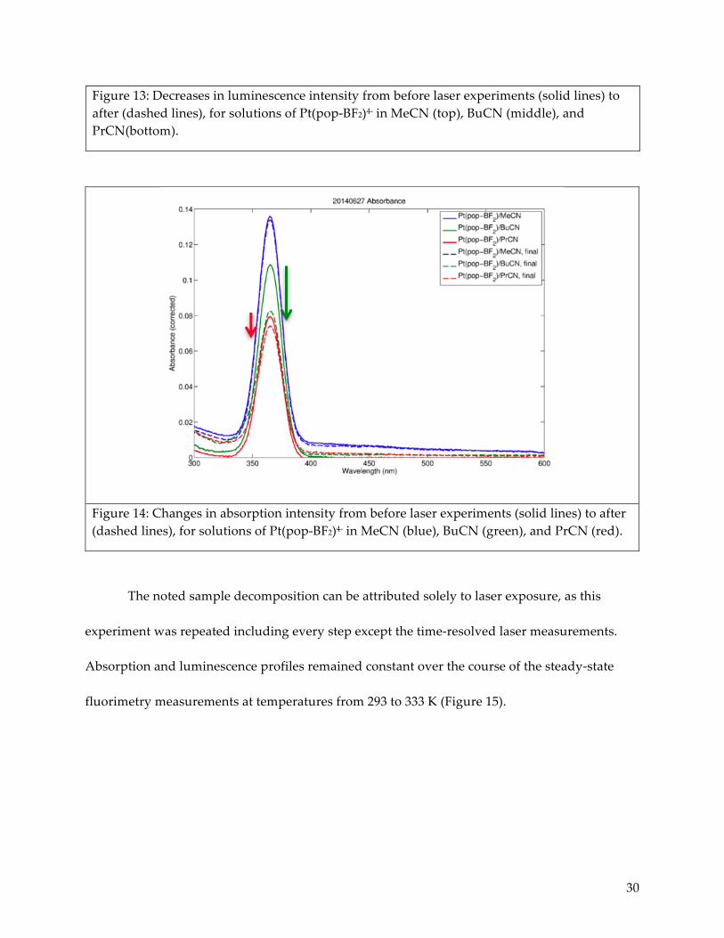
Figure 14: Changes in absorption intensity from before laser experiments (solid lines) to after (dashed lines), for solutions of Pt(pop-BF2)4- in MeCN (blue), BuCN (green), and PrCN (red).
The noted sample decomposition can be attributed solely to laser exposure, as this
experiment was repeated including every step except the time-resolved laser measurements.
Absorption and luminescence profiles remained constant over the course of the steady-state
fluorimetry measurements at temperatures from 293 to 333 K (Figure 15).
Figure 13: Decreases in luminescence intensity from before laser experiments (solid lines) to after (dashed lines), for solutions of Pt(pop-BF2)4- in MeCN (top), BuCN (middle), and PrCN(bottom).

31
Steady-state luminescence spectra Absorption spectra
Figure 15: Temperature-dependent measurements excluding the time-resolved laser experimental portion indicates Pt(pop-BF2)4- stability in MeCN (top), BuCN (middle), and PrCN (bottom).
32
2.4 Materials and methods
Unless otherwise noted, all reagents were obtained from Sigma-Aldrich and used without further
purification; all water used was deionized. All manipulations involving Pt(pop-BF2)4- were
carried out with standard air-free techniques in an inert-atmosphere glovebox or by utilizing a
vacuum manifold. Solvents were dried using activated alumina columns according to Grubbs’
method.18 Anhydrous acetonitrile was stored over activated 3 Å molecular sieves; all other
anhydrous solvents were stored over activated 4 Å molecular sieves.16 Molecular sieves were
activated by heating to 200 ºC under reduced pressure for 4 hours.
Phosphorous acid, H3PO3
Phosphorous acid was prepared by adding 15.6 g phosphorus trichloride (PCl3) to 40 mL
dichloromethane in a round-bottom flask in an ice bath. 6 mL water was added to a dropping
funnel and added to the stirring solution of PCl3 over 30 minutes. The flask was removed from
the ice bath and stirred at room temperature for 90 minutes. The dichloromethane was removed
under reduced pressure and the remaining fluffy white solid was transferred to a vial and stored
in a desiccator.
It is important to use a slight excess of PCl3 in order to obtain a solid product. Excess water
in the reaction will result in the formation of a thick, colorless oil; the H3PO3 product may be
recovered from this oil via multiple solvent extractions using CH2Cl2.
The 31P NMR exhibits a single peak at 5.86 ppm.
33
This reaction has been successfully scaled up to produce ~40 g of H3PO3 at a time;
however, extreme care must be taken to add the water slowly to avoid dangerous exotherms.
Furthermore, given the large amount of HCl gas produced at this scale, it is recommended to
route the evolved gas through a bubbler filled with ice and an aqueous solution of either sodium
bicarbonate or sodium hydroxide.
K4Pt(pop)
The water-soluble potassium salt of Pt(pop)4- was prepared by dissolving 0.326 g potassium
tetrachloroplatinate (K2PtCl4) in 10 mL water. 1.48 g phosphorus acid (as prepared in 2.4.1) was
dissolved in another 10 mL of water.ii The two solutions were mixed in a petri dish to give a light
red solution; this was held over a boiling water bath for three hours to yield a lightly-colored
yellow-brown solution. The petri dish was refilled with water every 30 minutes to maintain
solution volume. The dish was transferred to a modified vacuum oven set to 110 ºC for three
hours. This modified oven, rather than pulling vacuum, blew a constant stream of air through the
oven to purge out evolved hydrochloric acid. The resulting bright yellow solid was suspended in
methanol, isolated on a glass frit, and rinsed with copious methanol and diethyl ether. The
isolated solid was collected and dried under vacuum. The isolated solid may range in color from
bright yellowish-green to dark purple; when dissolved in water, the expected yellow-green
ii Commercially available phosphorous acid is often contaminated with water, as phosphorous acid is quite hygroscopic. Purchased phosphorous acid may be used for this synthesis, but yields may be adversely affected.
34
luminescent solution is reliably obtained. It has been proposed that the dark purple color is
caused by a small amount of a highly colored impurity.5
31P NMR exhibits a singlet at 67.1 ppm flanked by satellite peaks at 76.6 and 57.6 ppm
caused by coupling to the compound’s 195Pt atoms (1JPt-P = 3025 Hz, 33% abundance).
[TBA]4[Pt(pop)]
The tetrabutylammonium (TBA) salt of Pt(pop) was prepared by dissolving 0.35 g K4[Pt(pop)] in
4 mL water. 2.5 g (a 30-fold excess) tetrabutylammonium chloride ([(n-Bu)4N]Cl) was added to
the solution and stirred for one hour at room temperature. In the dark, the syrupy aqueous
solution was extracted with three 50 mL aliquots of dichloromethane and the organic layer was
concentrated under vacuum to a volume of 5 mL. 50 mL ethyl acetate was added to induce
precipitation of a bright yellow-green powder. The powder was isolated on a glass frit and dried
under vacuum.
31P NMR exhibits a single peak at 67.8 ppm flanked with the previously described 195Pt
coupling satellites. In the presence of light, Pt(pop)4- reacts with dichloromethane to form the
chloride adduct, which exhibits a single peak at 30.1 ppm in the 31P NMR spectrum.19 The
presence of this peak indicates a crude product which must be purified via recrystallization in
the dark from a concentrated CH2Cl2 solution layered with ethyl acetate.
[Ph4P]4[Pt(pop)]

35
The tetraphenylphosphonium (Ph4P+) salt of Pt(pop)4- may be prepared by a similar salt
metathesis procedure to that described in 2.4.3. Briefly, 1.2 g Ph4PCl was dissolved in 20 mL water
and 0.28 g K4Pt(pop) was dissolved in 50 mL water; both solutions were sparged with nitrogen
for 15 minutes. The tetraphenylphosphonium chloride solution was then added to the Pt(pop)4-
solution and a light yellow solid precipitated immediately. The solid was isolated via vacuum
filtration through fine glass-fiber filter paper and dried under vacuum.
Crystals suitable for X-ray diffraction analysis (bright yellow-green needles) were grown
from slow evaporation of a dilute methanol solution of the product. The 31P NMR exhibited a
single peak at 66.83 ppm, flanked by the previously discussed 195Pt satellite peaks.
[Ph4As]4[Pt(pop)]
The tetraphenylarsonium (Ph4As+) salt of Pt(pop)4- may be prepared in a similar salt metathesis
procedure to that described in 2.4.4. Briefly, 0.93 g Ph4AsCl was dissolved in 20 mL water and
0.34 g K4Pt(pop) was dissolved in 50 mL water; both solutions were sparged with nitrogen for 15
minutes. The tetraphenylphosphonium solution was then added to the Pt(pop)4- solution and a
light yellow solid precipitated immediately. The solid was isolated via vacuum filtration through
fine glass-fiber filter paper and dried under vacuum.
The 31P NMR exhibited a single peak at 67.1 ppm, flanked by the previously discussed
195Pt satellite peaks.
[Pt(pop-BF2)]4-
36
[R]4[Pt(pop-BF2)], where R = Ph4P+, (n-Bu)4N+, or Ph4As+, was prepared by adding 0.3 – 0.6 g of the
appropriate Pt(pop)4- salt to a 10 mL Schlenk flask. After sparging with dry argon for 15 minutes,
a syringe was used to add 3.5 mL boron trifluoride diethyletherate (BF3•Et2O ) to the flask through
a rubber septum. Under positive argon flow, the rubber septum was replaced with a ground-
glass stopper; the reaction was then left stirring under a static blanket of argon for six hours
(although the reaction may be left stirring for multiple days with no decomposition). The
remaining BF3•Et2O was removed under reduced pressure in a 40 ºC water bath. The BF3•Et2O
was condensed into an ice-cooled pre-trap immediately in line after the Schlenk flask. If a pre-
trap is not used, BF3•Et2O will condense inside the vacuum tubing and/or the Schlenk line itself,
causing contamination and presenting a significant health and safety hazard to researchers.
Removal of solvent yielded a bright yellow-green powder. The Schlenk flask containing the
product was sealed under nitrogen and taken into an inert-atmosphere glovebox; the product
was then suspended in dry tetrahydrofuran (THF), filtered through a glass frit, and rinsed with
copious THF. The isolated product was dried under vacuum and recrystallized via slow
evaporation of diethylether into a saturated acetonitrile solution to yield bright yellow-green
luminescent crystalline blocks.
The 31P NMR exhibits a single peak at ≈58.8 ppm (depending on the cation; see section 2.5)
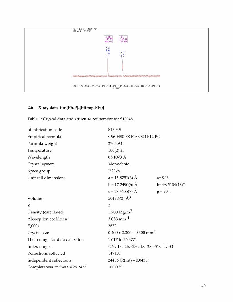
together with the aforementioned 195Pt coupling satellite peaks (1JPt-P ≅ 3126 – 3136 Hz). The 19F
NMR exhibits two doublets at 133.5 ppm (1J = 60 Hz) and 138.7 ppm (1J = 60 Hz).
X-ray structure determination of [Ph4P]4[Pt(pop-BF2)]
Low-temperature diffraction data (f-and w-scans) were collected on a Bruker three-circle
diffractometer coupled to a Bruker Smart 1000 CCD detector with graphite monochromated Mo

37
Ka radiation (l = 0.71073 Å) for the structure of [Ph4P]4[Pt(pop-BF2)]. The structure was solved by
direct methods using SHELXS20 and refined against F2 on all data by full-matrix least squares with
SHELXL-201321 using established refinement techniques.22 All non-hydrogen atoms were refined
anisotropically. All hydrogen atoms were included into the model at geometrically calculated
positions and refined using a riding model. The isotropic displacement parameters of all
hydrogen atoms were fixed to 1.2 times the U value of the atoms they are linked to (1.5 times for
methyl groups). Data are presented in section 2.6.
Steady-state quenching experiments
Steady-state emission spectra were recorded on a Jobin Yvon Spex Fluorolog-3-11. A 450-W
xenon arc lamp was used as the excitation source with a single monochromator providing
wavelength selection. Right-angle light emission was sorted using a single monochromator and
fed into a Hamamatsu R928P photomultiplier tube with photon counting. Short and long pass
filters were used where appropriate. Spectra were recorded on Datamax software.2 Variable-
temperature experiments were performed using a Peltier-cooled circulating water bath.
Temperature-dependent lifetime experiments: Picosecond laser data2
An IBH 5000 U instrument equipped with a cooled Hamamatsu R3809U-50 microchannel plate
photomultiplier was used. Samples were excited at 355 nm with an IBH NanoLED-03 diode
laser (∼80 ps fwhm, repetition rate 500 kHz). For fluorescence decay measurements, the
emission monochromator was set to ≈405 ± 4 nm, preceded by a 390 nm long-pass cutoff filter to
remove stray excitation light. Magic angle between the excitation and emission polarization
directions was used for all experiments. Variable-temperature experiments were performed

38
using a Peltier-cooled circulating water bath. Data manipulation was performed and plotted
using MATLAB R2015a (Mathworks, Inc.).
2.5 NMR spectra
All NMR spectra were recorded in the Caltech Liquid NMR facility using a Varian 400 MHz
spectrometer with a broadband auto-tune OneProbe (“Siena”). All 31P spectra were externally
referenced to 85% phosphoric acid. Spectra were processed using the MestReNova software
suite.23
K4Pt(pop)
1H 31P
[(n-Bu)4P]4[Pt(pop-BF2)]
1H 31P

39
19F
[Ph4P]4[Pt(pop-BF2)]
1H 31P
19F
40
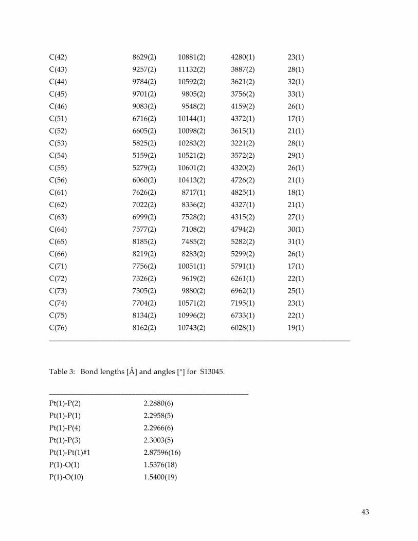
2.6 X-ray data for [Ph4P]4[Pt(pop-BF2)]
Table 1: Crystal data and structure refinement for S13045.
Identification code S13045 Empirical formula C96 H80 B8 F16 O20 P12 Pt2 Formula weight 2705.90 Temperature 100(2) K Wavelength 0.71073 Å Crystal system Monoclinic Space group P 21/n Unit cell dimensions a = 15.8751(6) Å a= 90°. b = 17.2490(6) Å b= 98.5184(18)°. c = 18.6455(7) Å g = 90°. Volume 5049.4(3) Å3 Z 2 Density (calculated) 1.780 Mg/m3 Absorption coefficient 3.058 mm-1 F(000) 2672 Crystal size 0.400 x 0.300 x 0.300 mm3 Theta range for data collection 1.617 to 36.377°. Index ranges -26<=h<=26, -28<=k<=28, -31<=l<=30 Reflections collected 149401 Independent reflections 24436 [R(int) = 0.0435] Completeness to theta = 25.242° 100.0 %
41
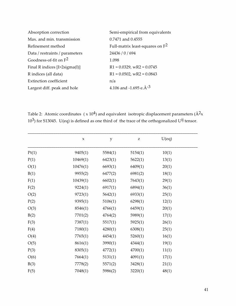
Absorption correction Semi-empirical from equivalents Max. and min. transmission 0.7471 and 0.4555 Refinement method Full-matrix least-squares on F2 Data / restraints / parameters 24436 / 0 / 694 Goodness-of-fit on F2 1.098 Final R indices [I>2sigma(I)] R1 = 0.0329, wR2 = 0.0745 R indices (all data) R1 = 0.0502, wR2 = 0.0843 Extinction coefficient n/a Largest diff. peak and hole 4.106 and -1.695 e.Å-3
Table 2: Atomic coordinates ( x 104) and equivalent isotropic displacement parameters (Å2x 10³) for S13045. U(eq) is defined as one third of the trace of the orthogonalized Uij tensor.
________________________________________________________________________________ x y z U(eq) ________________________________________________________________________________ Pt(1) 9405(1) 5584(1) 5154(1) 10(1) P(1) 10469(1) 6423(1) 5622(1) 13(1) O(1) 10476(1) 6693(1) 6409(1) 20(1) B(1) 9955(2) 6477(2) 6981(2) 18(1) F(1) 10439(1) 6602(1) 7643(1) 29(1) F(2) 9224(1) 6917(1) 6894(1) 36(1) O(2) 9723(1) 5642(1) 6933(1) 25(1) P(2) 9395(1) 5106(1) 6298(1) 12(1) O(3) 8546(1) 4766(1) 6459(1) 20(1) B(2) 7701(2) 4764(2) 5989(1) 17(1) F(3) 7387(1) 5517(1) 5925(1) 26(1) F(4) 7180(1) 4280(1) 6308(1) 25(1) O(4) 7765(1) 4454(1) 5260(1) 16(1) O(5) 8616(1) 3990(1) 4344(1) 19(1) P(3) 8305(1) 4772(1) 4700(1) 11(1) O(6) 7664(1) 5131(1) 4091(1) 17(1) B(3) 7778(2) 5571(2) 3428(1) 21(1) F(5) 7048(1) 5986(2) 3220(1) 48(1)

42
F(6) 7936(2) 5054(1) 2905(1) 53(1) O(7) 8499(1) 6125(1) 3550(1) 18(1) O(8) 9968(1) 5623(1) 3541(1) 22(1) P(4) 9377(1) 6106(1) 4018(1) 12(1) O(9) 9694(1) 6949(1) 3993(1) 21(1) B(4) 10448(2) 7337(2) 4408(2) 20(1) F(7) 10361(1) 8113(1) 4301(1) 40(1) F(8) 11185(1) 7060(2) 4179(1) 40(1) O(10) 10521(1) 7184(1) 5200(1) 21(1) P(5) 9558(1) 8187(1) 1153(1) 15(1) C(1) 8687(1) 7969(1) 1629(1) 17(1) C(2) 8310(2) 8544(2) 2001(2) 24(1) C(3) 7631(2) 8345(2) 2358(2) 31(1) C(4) 7350(2) 7588(2) 2365(2) 26(1) C(5) 7729(2) 7018(2) 1999(2) 22(1) C(6) 8392(2) 7207(2) 1620(1) 21(1) C(11) 10533(1) 7784(1) 1620(1) 16(1) C(12) 10527(2) 7269(1) 2200(1) 18(1) C(13) 11292(2) 6954(2) 2543(1) 21(1) C(14) 12055(2) 7155(2) 2317(1) 22(1) C(15) 12068(2) 7682(2) 1749(1) 21(1) C(16) 11310(2) 7994(2) 1402(1) 19(1) C(21) 9306(2) 7764(1) 264(1) 17(1) C(22) 9926(2) 7397(2) -79(1) 20(1) C(23) 9702(2) 7082(2) -768(1) 23(1) C(24) 8865(2) 7133(2) -1117(2) 25(1) C(25) 8250(2) 7498(2) -781(2) 26(1) C(26) 8465(2) 7814(2) -90(1) 21(1) C(31) 9693(2) 9215(1) 1105(1) 17(1) C(32) 9219(2) 9643(2) 548(1) 21(1) C(33) 9288(2) 10448(2) 554(2) 26(1) C(34) 9826(2) 10823(2) 1099(2) 29(1) C(35) 10305(2) 10396(2) 1648(2) 28(1) C(36) 10234(2) 9595(2) 1658(2) 24(1) P(6) 7680(1) 9757(1) 4861(1) 15(1) C(41) 8545(2) 10091(2) 4419(1) 19(1)
43
C(42) 8629(2) 10881(2) 4280(1) 23(1) C(43) 9257(2) 11132(2) 3887(2) 28(1) C(44) 9784(2) 10592(2) 3621(2) 32(1) C(45) 9701(2) 9805(2) 3756(2) 33(1) C(46) 9083(2) 9548(2) 4159(2) 26(1) C(51) 6716(2) 10144(1) 4372(1) 17(1) C(52) 6605(2) 10098(2) 3615(1) 21(1) C(53) 5825(2) 10283(2) 3221(2) 28(1) C(54) 5159(2) 10521(2) 3572(2) 29(1) C(55) 5279(2) 10601(2) 4320(2) 26(1) C(56) 6060(2) 10413(2) 4726(2) 21(1) C(61) 7626(2) 8717(1) 4825(1) 18(1) C(62) 7022(2) 8336(2) 4327(1) 21(1) C(63) 6999(2) 7528(2) 4315(2) 27(1) C(64) 7577(2) 7108(2) 4794(2) 30(1) C(65) 8185(2) 7485(2) 5282(2) 31(1) C(66) 8219(2) 8283(2) 5299(2) 26(1) C(71) 7756(2) 10051(1) 5791(1) 17(1) C(72) 7326(2) 9619(2) 6261(1) 22(1) C(73) 7305(2) 9880(2) 6962(1) 25(1) C(74) 7704(2) 10571(2) 7195(1) 23(1) C(75) 8134(2) 10996(2) 6733(1) 22(1) C(76) 8162(2) 10743(2) 6028(1) 19(1) ________________________________________________________________________________
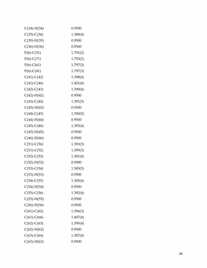
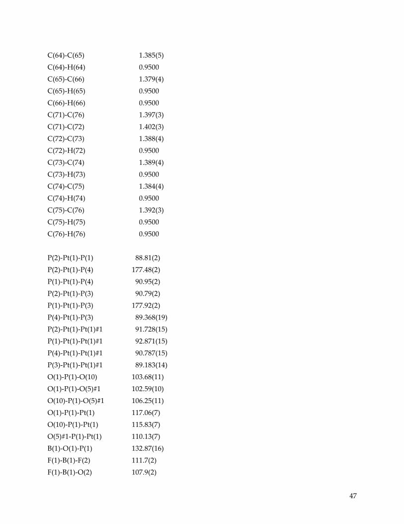
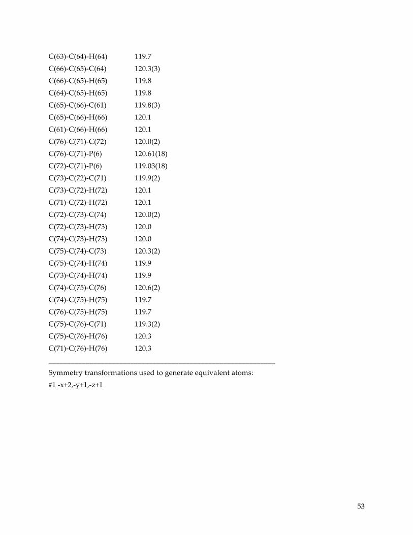
Table 3: Bond lengths [Å] and angles [°] for S13045.
_____________________________________________________ Pt(1)-P(2) 2.2880(6) Pt(1)-P(1) 2.2958(5) Pt(1)-P(4) 2.2966(6) Pt(1)-P(3) 2.3003(5) Pt(1)-Pt(1)#1 2.87596(16) P(1)-O(1) 1.5376(18) P(1)-O(10) 1.5400(19)

44
P(1)-O(5)#1 1.6110(18) O(1)-B(1) 1.490(3) B(1)-F(1) 1.371(3) B(1)-F(2) 1.377(3) B(1)-O(2) 1.486(3) O(2)-P(2) 1.5318(18) P(2)-O(3) 1.5392(18) P(2)-O(8)#1 1.6145(18) O(3)-B(2) 1.491(3) B(2)-F(4) 1.372(3) B(2)-F(3) 1.388(3) B(2)-O(4) 1.478(3) O(4)-P(3) 1.5453(17) O(5)-P(1)#1 1.6110(18) O(5)-P(3) 1.6134(18) P(3)-O(6) 1.5389(17) O(6)-B(3) 1.483(3) B(3)-F(5) 1.368(4) B(3)-F(6) 1.373(4) B(3)-O(7) 1.483(3) O(7)-P(4) 1.5308(17) O(8)-P(2)#1 1.6146(18) O(8)-P(4) 1.6156(19) P(4)-O(9) 1.5431(18) O(9)-B(4) 1.485(3) B(4)-F(7) 1.357(3) B(4)-F(8) 1.388(4) B(4)-O(10) 1.487(3) P(5)-C(31) 1.789(2) P(5)-C(1) 1.791(2) P(5)-C(11) 1.799(2) P(5)-C(21) 1.801(2) C(1)-C(6) 1.395(3) C(1)-C(2) 1.395(3) C(2)-C(3) 1.390(4) C(2)-H(2) 0.9500

45
C(3)-C(4) 1.381(4) C(3)-H(3) 0.9500 C(4)-C(5) 1.383(4) C(4)-H(4) 0.9500 C(5)-C(6) 1.391(3) C(5)-H(5) 0.9500 C(6)-H(6) 0.9500 C(11)-C(12) 1.401(3) C(11)-C(16) 1.402(3) C(12)-C(13) 1.396(3) C(12)-H(12) 0.9500 C(13)-C(14) 1.384(4) C(13)-H(13) 0.9500 C(14)-C(15) 1.398(4) C(14)-H(14) 0.9500 C(15)-C(16) 1.388(3) C(15)-H(15) 0.9500 C(16)-H(16) 0.9500 C(21)-C(22) 1.402(3) C(21)-C(26) 1.403(3) C(22)-C(23) 1.391(4) C(22)-H(22) 0.9500 C(23)-C(24) 1.394(4) C(23)-H(23) 0.9500 C(24)-C(25) 1.386(4) C(24)-H(24) 0.9500 C(25)-C(26) 1.393(4) C(25)-H(25) 0.9500 C(26)-H(26) 0.9500 C(31)-C(32) 1.400(3) C(31)-C(36) 1.403(4) C(32)-C(33) 1.393(4) C(32)-H(32) 0.9500 C(33)-C(34) 1.387(4) C(33)-H(33) 0.9500 C(34)-C(35) 1.392(4)
46
C(34)-H(34) 0.9500 C(35)-C(36) 1.388(4) C(35)-H(35) 0.9500 C(36)-H(36) 0.9500 P(6)-C(51) 1.791(2) P(6)-C(71) 1.793(2) P(6)-C(61) 1.797(3) P(6)-C(41) 1.797(3) C(41)-C(42) 1.398(4) C(41)-C(46) 1.401(4) C(42)-C(43) 1.390(4) C(42)-H(42) 0.9500 C(43)-C(44) 1.391(5) C(43)-H(43) 0.9500 C(44)-C(45) 1.390(5) C(44)-H(44) 0.9500 C(45)-C(46) 1.393(4) C(45)-H(45) 0.9500 C(46)-H(46) 0.9500 C(51)-C(56) 1.393(3) C(51)-C(52) 1.399(3) C(52)-C(53) 1.381(4) C(52)-H(52) 0.9500 C(53)-C(54) 1.385(5) C(53)-H(53) 0.9500 C(54)-C(55) 1.385(4) C(54)-H(54) 0.9500 C(55)-C(56) 1.392(4) C(55)-H(55) 0.9500 C(56)-H(56) 0.9500 C(61)-C(62) 1.396(3) C(61)-C(66) 1.407(4) C(62)-C(63) 1.395(4) C(62)-H(62) 0.9500 C(63)-C(64) 1.387(4) C(63)-H(63) 0.9500
47
C(64)-C(65) 1.385(5) C(64)-H(64) 0.9500 C(65)-C(66) 1.379(4) C(65)-H(65) 0.9500 C(66)-H(66) 0.9500 C(71)-C(76) 1.397(3) C(71)-C(72) 1.402(3) C(72)-C(73) 1.388(4) C(72)-H(72) 0.9500 C(73)-C(74) 1.389(4) C(73)-H(73) 0.9500 C(74)-C(75) 1.384(4) C(74)-H(74) 0.9500 C(75)-C(76) 1.392(3) C(75)-H(75) 0.9500 C(76)-H(76) 0.9500 P(2)-Pt(1)-P(1) 88.81(2) P(2)-Pt(1)-P(4) 177.48(2) P(1)-Pt(1)-P(4) 90.95(2) P(2)-Pt(1)-P(3) 90.79(2) P(1)-Pt(1)-P(3) 177.92(2) P(4)-Pt(1)-P(3) 89.368(19) P(2)-Pt(1)-Pt(1)#1 91.728(15) P(1)-Pt(1)-Pt(1)#1 92.871(15) P(4)-Pt(1)-Pt(1)#1 90.787(15) P(3)-Pt(1)-Pt(1)#1 89.183(14) O(1)-P(1)-O(10) 103.68(11) O(1)-P(1)-O(5)#1 102.59(10) O(10)-P(1)-O(5)#1 106.25(11) O(1)-P(1)-Pt(1) 117.06(7) O(10)-P(1)-Pt(1) 115.83(7) O(5)#1-P(1)-Pt(1) 110.13(7) B(1)-O(1)-P(1) 132.87(16) F(1)-B(1)-F(2) 111.7(2) F(1)-B(1)-O(2) 107.9(2)

48
F(2)-B(1)-O(2) 109.3(2) F(1)-B(1)-O(1) 108.0(2) F(2)-B(1)-O(1) 108.9(2) O(2)-B(1)-O(1) 111.0(2) B(1)-O(2)-P(2) 133.14(17) O(2)-P(2)-O(3) 106.65(11) O(2)-P(2)-O(8)#1 101.19(12) O(3)-P(2)-O(8)#1 102.03(11) O(2)-P(2)-Pt(1) 117.08(8) O(3)-P(2)-Pt(1) 116.54(7) O(8)#1-P(2)-Pt(1) 111.28(7) B(2)-O(3)-P(2) 128.56(15) F(4)-B(2)-F(3) 112.1(2) F(4)-B(2)-O(4) 107.8(2) F(3)-B(2)-O(4) 109.4(2) F(4)-B(2)-O(3) 107.02(19) F(3)-B(2)-O(3) 109.2(2) O(4)-B(2)-O(3) 111.26(18) B(2)-O(4)-P(3) 127.80(15) P(1)#1-O(5)-P(3) 133.11(11) O(6)-P(3)-O(4) 105.61(9) O(6)-P(3)-O(5) 104.04(10) O(4)-P(3)-O(5) 102.45(10) O(6)-P(3)-Pt(1) 114.17(7) O(4)-P(3)-Pt(1) 115.76(7) O(5)-P(3)-Pt(1) 113.45(6) B(3)-O(6)-P(3) 132.22(16) F(5)-B(3)-F(6) 111.9(3) F(5)-B(3)-O(6) 107.5(2) F(6)-B(3)-O(6) 108.6(2) F(5)-B(3)-O(7) 108.0(2) F(6)-B(3)-O(7) 108.0(2) O(6)-B(3)-O(7) 112.89(19) B(3)-O(7)-P(4) 133.61(16) P(2)#1-O(8)-P(4) 134.28(12) O(7)-P(4)-O(9) 103.65(10)

49
O(7)-P(4)-O(8) 104.57(10) O(9)-P(4)-O(8) 104.47(11) O(7)-P(4)-Pt(1) 115.25(7) O(9)-P(4)-Pt(1) 115.83(7) O(8)-P(4)-Pt(1) 111.83(7) B(4)-O(9)-P(4) 130.59(17) F(7)-B(4)-F(8) 111.5(2) F(7)-B(4)-O(9) 108.1(2) F(8)-B(4)-O(9) 109.6(2) F(7)-B(4)-O(10) 108.1(2) F(8)-B(4)-O(10) 107.4(2) O(9)-B(4)-O(10) 112.1(2) B(4)-O(10)-P(1) 131.03(16) C(31)-P(5)-C(1) 109.89(11) C(31)-P(5)-C(11) 107.84(11) C(1)-P(5)-C(11) 110.57(11) C(31)-P(5)-C(21) 111.49(11) C(1)-P(5)-C(21) 106.81(11) C(11)-P(5)-C(21) 110.26(11) C(6)-C(1)-C(2) 120.6(2) C(6)-C(1)-P(5) 118.29(18) C(2)-C(1)-P(5) 121.14(19) C(3)-C(2)-C(1) 118.8(3) C(3)-C(2)-H(2) 120.6 C(1)-C(2)-H(2) 120.6 C(4)-C(3)-C(2) 120.8(3) C(4)-C(3)-H(3) 119.6 C(2)-C(3)-H(3) 119.6 C(3)-C(4)-C(5) 120.2(3) C(3)-C(4)-H(4) 119.9 C(5)-C(4)-H(4) 119.9 C(4)-C(5)-C(6) 120.1(3) C(4)-C(5)-H(5) 120.0 C(6)-C(5)-H(5) 120.0 C(5)-C(6)-C(1) 119.5(2) C(5)-C(6)-H(6) 120.3

50
C(1)-C(6)-H(6) 120.3 C(12)-C(11)-C(16) 119.6(2) C(12)-C(11)-P(5) 121.00(18) C(16)-C(11)-P(5) 119.36(18) C(13)-C(12)-C(11) 119.7(2) C(13)-C(12)-H(12) 120.1 C(11)-C(12)-H(12) 120.1 C(14)-C(13)-C(12) 120.3(2) C(14)-C(13)-H(13) 119.9 C(12)-C(13)-H(13) 119.9 C(13)-C(14)-C(15) 120.4(2) C(13)-C(14)-H(14) 119.8 C(15)-C(14)-H(14) 119.8 C(16)-C(15)-C(14) 119.7(2) C(16)-C(15)-H(15) 120.1 C(14)-C(15)-H(15) 120.1 C(15)-C(16)-C(11) 120.2(2) C(15)-C(16)-H(16) 119.9 C(11)-C(16)-H(16) 119.9 C(22)-C(21)-C(26) 119.8(2) C(22)-C(21)-P(5) 121.85(18) C(26)-C(21)-P(5) 118.36(19) C(23)-C(22)-C(21) 119.7(2) C(23)-C(22)-H(22) 120.1 C(21)-C(22)-H(22) 120.1 C(22)-C(23)-C(24) 120.2(2) C(22)-C(23)-H(23) 119.9 C(24)-C(23)-H(23) 119.9 C(25)-C(24)-C(23) 120.3(2) C(25)-C(24)-H(24) 119.8 C(23)-C(24)-H(24) 119.8 C(24)-C(25)-C(26) 120.2(2) C(24)-C(25)-H(25) 119.9 C(26)-C(25)-H(25) 119.9 C(25)-C(26)-C(21) 119.8(2) C(25)-C(26)-H(26) 120.1

51
C(21)-C(26)-H(26) 120.1 C(32)-C(31)-C(36) 120.1(2) C(32)-C(31)-P(5) 120.34(19) C(36)-C(31)-P(5) 119.37(19) C(33)-C(32)-C(31) 119.2(3) C(33)-C(32)-H(32) 120.4 C(31)-C(32)-H(32) 120.4 C(34)-C(33)-C(32) 120.7(3) C(34)-C(33)-H(33) 119.7 C(32)-C(33)-H(33) 119.7 C(33)-C(34)-C(35) 120.2(3) C(33)-C(34)-H(34) 119.9 C(35)-C(34)-H(34) 119.9 C(36)-C(35)-C(34) 120.0(3) C(36)-C(35)-H(35) 120.0 C(34)-C(35)-H(35) 120.0 C(35)-C(36)-C(31) 119.9(3) C(35)-C(36)-H(36) 120.1 C(31)-C(36)-H(36) 120.1 C(51)-P(6)-C(71) 108.47(11) C(51)-P(6)-C(61) 108.71(11) C(71)-P(6)-C(61) 108.29(11) C(51)-P(6)-C(41) 107.51(11) C(71)-P(6)-C(41) 113.97(11) C(61)-P(6)-C(41) 109.77(12) C(42)-C(41)-C(46) 120.4(2) C(42)-C(41)-P(6) 119.87(19) C(46)-C(41)-P(6) 119.4(2) C(43)-C(42)-C(41) 119.8(3) C(43)-C(42)-H(42) 120.1 C(41)-C(42)-H(42) 120.1 C(42)-C(43)-C(44) 119.7(3) C(42)-C(43)-H(43) 120.1 C(44)-C(43)-H(43) 120.1 C(45)-C(44)-C(43) 120.7(3) C(45)-C(44)-H(44) 119.6

52
C(43)-C(44)-H(44) 119.6 C(44)-C(45)-C(46) 120.1(3) C(44)-C(45)-H(45) 120.0 C(46)-C(45)-H(45) 120.0 C(45)-C(46)-C(41) 119.2(3) C(45)-C(46)-H(46) 120.4 C(41)-C(46)-H(46) 120.4 C(56)-C(51)-C(52) 120.4(2) C(56)-C(51)-P(6) 121.73(18) C(52)-C(51)-P(6) 117.56(19) C(53)-C(52)-C(51) 119.5(3) C(53)-C(52)-H(52) 120.3 C(51)-C(52)-H(52) 120.3 C(52)-C(53)-C(54) 120.3(3) C(52)-C(53)-H(53) 119.8 C(54)-C(53)-H(53) 119.8 C(53)-C(54)-C(55) 120.2(2) C(53)-C(54)-H(54) 119.9 C(55)-C(54)-H(54) 119.9 C(54)-C(55)-C(56) 120.3(3) C(54)-C(55)-H(55) 119.9 C(56)-C(55)-H(55) 119.9 C(55)-C(56)-C(51) 119.2(2) C(55)-C(56)-H(56) 120.4 C(51)-C(56)-H(56) 120.4 C(62)-C(61)-C(66) 119.8(2) C(62)-C(61)-P(6) 121.26(19) C(66)-C(61)-P(6) 118.9(2) C(63)-C(62)-C(61) 119.7(3) C(63)-C(62)-H(62) 120.2 C(61)-C(62)-H(62) 120.2 C(64)-C(63)-C(62) 119.9(3) C(64)-C(63)-H(63) 120.1 C(62)-C(63)-H(63) 120.1 C(65)-C(64)-C(63) 120.6(3) C(65)-C(64)-H(64) 119.7
53
C(63)-C(64)-H(64) 119.7 C(66)-C(65)-C(64) 120.3(3) C(66)-C(65)-H(65) 119.8 C(64)-C(65)-H(65) 119.8 C(65)-C(66)-C(61) 119.8(3) C(65)-C(66)-H(66) 120.1 C(61)-C(66)-H(66) 120.1 C(76)-C(71)-C(72) 120.0(2) C(76)-C(71)-P(6) 120.61(18) C(72)-C(71)-P(6) 119.03(18) C(73)-C(72)-C(71) 119.9(2) C(73)-C(72)-H(72) 120.1 C(71)-C(72)-H(72) 120.1 C(72)-C(73)-C(74) 120.0(2) C(72)-C(73)-H(73) 120.0 C(74)-C(73)-H(73) 120.0 C(75)-C(74)-C(73) 120.3(2) C(75)-C(74)-H(74) 119.9 C(73)-C(74)-H(74) 119.9 C(74)-C(75)-C(76) 120.6(2) C(74)-C(75)-H(75) 119.7 C(76)-C(75)-H(75) 119.7 C(75)-C(76)-C(71) 119.3(2) C(75)-C(76)-H(76) 120.3 C(71)-C(76)-H(76) 120.3 _____________________________________________________________ Symmetry transformations used to generate equivalent atoms: #1 -x+2,-y+1,-z+1

54
Table 4: Anisotropic displacement parameters (Å2x 10³) for S13045. The anisotropic
displacement factor exponent takes the form: -2p2[ h2 a*2U11 + ... + 2 h k a* b* U12 ] ______________________________________________________________________________ U11 U22 U33 U23 U13 U12 ______________________________________________________________________________ Pt(1) 11(1) 10(1) 10(1) 0(1) 3(1) 0(1) P(1) 14(1) 11(1) 12(1) -1(1) 3(1) -2(1) O(1) 22(1) 22(1) 17(1) -10(1) 6(1) -6(1) B(1) 20(1) 21(1) 16(1) -6(1) 5(1) -3(1) F(1) 34(1) 35(1) 16(1) -9(1) 2(1) -10(1) F(2) 25(1) 42(1) 44(1) -3(1) 12(1) 11(1) O(2) 41(1) 24(1) 11(1) -3(1) 4(1) -13(1) P(2) 13(1) 15(1) 9(1) -1(1) 3(1) -1(1) O(3) 15(1) 30(1) 14(1) 6(1) 3(1) -3(1) B(2) 14(1) 22(1) 14(1) 1(1) 5(1) 1(1) F(3) 26(1) 25(1) 26(1) 0(1) 3(1) 10(1) F(4) 19(1) 39(1) 19(1) 3(1) 8(1) -9(1) O(4) 14(1) 20(1) 14(1) 1(1) 3(1) -5(1) O(5) 14(1) 17(1) 26(1) -10(1) 3(1) -1(1) P(3) 11(1) 13(1) 10(1) 0(1) 3(1) -1(1) O(6) 13(1) 20(1) 16(1) 4(1) 1(1) -2(1) B(3) 20(1) 26(1) 14(1) 6(1) -2(1) -8(1) F(5) 18(1) 64(2) 58(1) 41(1) -4(1) -5(1) F(6) 94(2) 44(1) 27(1) -18(1) 27(1) -39(1) O(7) 15(1) 21(1) 18(1) 6(1) -1(1) -3(1) O(8) 26(1) 28(1) 14(1) 6(1) 8(1) 12(1) P(4) 12(1) 13(1) 12(1) 2(1) 2(1) -1(1) O(9) 25(1) 17(1) 19(1) 5(1) -1(1) -6(1) B(4) 25(1) 17(1) 20(1) 2(1) 4(1) -6(1) F(7) 55(1) 20(1) 39(1) 10(1) -9(1) -13(1) F(8) 24(1) 67(2) 31(1) -5(1) 10(1) -3(1) O(10) 29(1) 13(1) 20(1) 0(1) 0(1) -5(1) P(5) 15(1) 15(1) 15(1) 2(1) 2(1) 0(1) C(1) 18(1) 18(1) 18(1) 2(1) 4(1) 2(1) C(2) 31(1) 19(1) 27(1) 2(1) 14(1) 3(1)

55
C(3) 40(2) 24(1) 34(2) 2(1) 23(1) 6(1) C(4) 27(1) 28(1) 27(1) 7(1) 13(1) 3(1) C(5) 21(1) 23(1) 24(1) 4(1) 5(1) -2(1) C(6) 21(1) 20(1) 23(1) 0(1) 6(1) -1(1) C(11) 17(1) 16(1) 16(1) 1(1) 2(1) 1(1) C(12) 20(1) 17(1) 16(1) 3(1) 2(1) 0(1) C(13) 25(1) 18(1) 18(1) 2(1) -2(1) 1(1) C(14) 22(1) 23(1) 21(1) -3(1) -2(1) 5(1) C(15) 16(1) 26(1) 21(1) -2(1) 1(1) 2(1) C(16) 18(1) 21(1) 18(1) 2(1) 3(1) 0(1) C(21) 18(1) 17(1) 16(1) 1(1) 2(1) 1(1) C(22) 19(1) 22(1) 19(1) 0(1) 4(1) 1(1) C(23) 25(1) 24(1) 21(1) -3(1) 6(1) -1(1) C(24) 29(1) 26(1) 21(1) -3(1) 2(1) -1(1) C(25) 23(1) 30(1) 22(1) -2(1) -4(1) 0(1) C(26) 19(1) 23(1) 21(1) -2(1) 0(1) 4(1) C(31) 17(1) 15(1) 20(1) 2(1) 3(1) 1(1) C(32) 17(1) 21(1) 24(1) 6(1) 3(1) 3(1) C(33) 24(1) 22(1) 34(1) 9(1) 8(1) 5(1) C(34) 30(1) 18(1) 41(2) 2(1) 13(1) 1(1) C(35) 31(1) 20(1) 34(1) -3(1) 4(1) -4(1) C(36) 26(1) 19(1) 25(1) 1(1) -1(1) -1(1) P(6) 18(1) 16(1) 12(1) -1(1) 2(1) 1(1) C(41) 20(1) 21(1) 16(1) -2(1) 4(1) 1(1) C(42) 28(1) 22(1) 20(1) -1(1) 7(1) -4(1) C(43) 34(1) 27(1) 26(1) 0(1) 10(1) -9(1) C(44) 25(1) 42(2) 33(1) -1(1) 11(1) -8(1) C(45) 25(1) 39(2) 39(2) -3(1) 16(1) 3(1) C(46) 24(1) 26(1) 31(1) 1(1) 10(1) 4(1) C(51) 19(1) 16(1) 15(1) -1(1) 0(1) 0(1) C(52) 26(1) 22(1) 15(1) 1(1) 0(1) 0(1) C(53) 31(1) 29(1) 21(1) 4(1) -7(1) -3(1) C(54) 22(1) 27(1) 34(1) 12(1) -6(1) -4(1) C(55) 19(1) 24(1) 34(1) 6(1) 4(1) 1(1) C(56) 19(1) 22(1) 22(1) 1(1) 4(1) 2(1) C(61) 22(1) 19(1) 16(1) 1(1) 5(1) 1(1)

56
C(62) 25(1) 17(1) 22(1) 1(1) 5(1) -1(1) C(63) 33(1) 18(1) 34(1) -4(1) 13(1) -4(1) C(64) 41(2) 16(1) 37(2) 2(1) 23(1) 5(1) C(65) 41(2) 22(1) 32(1) 6(1) 13(1) 12(1) C(66) 31(1) 26(1) 21(1) 1(1) 3(1) 9(1) C(71) 18(1) 20(1) 13(1) -1(1) 1(1) -1(1) C(72) 28(1) 23(1) 16(1) -1(1) 4(1) -8(1) C(73) 31(1) 28(1) 16(1) -2(1) 6(1) -7(1) C(74) 30(1) 26(1) 13(1) -3(1) 2(1) -2(1) C(75) 28(1) 20(1) 16(1) -3(1) 0(1) -3(1) C(76) 22(1) 20(1) 16(1) -2(1) 1(1) -2(1) ______________________________________________________________________________
Table 5: Hydrogen coordinates ( x 104) and isotropic displacement parameters (Å2x 10 3)
for S13045. ________________________________________________________________________________ x y z U(eq) ________________________________________________________________________________ H(2) 8513 9063 2011 29 H(3) 7357 8735 2600 37 H(4) 6896 7458 2622 32 H(5) 7536 6497 2007 27 H(6) 8642 6820 1356 25 H(12) 10005 7134 2360 21 H(13) 11289 6600 2933 25 H(14) 12572 6934 2549 27 H(15) 12594 7826 1602 25 H(16) 11317 8350 1014 23 H(22) 10498 7363 158 24 H(23) 10121 6832 -1001 27 H(24) 8714 6917 -1587 30 H(25) 7680 7532 -1022 31 H(26) 8042 8062 140 25

57
H(32) 8855 9388 170 25 H(33) 8963 10743 181 32 H(34) 9867 11372 1099 34 H(35) 10681 10654 2016 34 H(36) 10550 9304 2039 29 H(42) 8259 11246 4453 28 H(43) 9325 11669 3800 34 H(44) 10205 10763 3345 39 H(45) 10066 9443 3573 40 H(46) 9027 9012 4255 31 H(52) 7064 9941 3373 25 H(53) 5744 10246 2707 34 H(54) 4618 10631 3299 34 H(55) 4827 10784 4556 31 H(56) 6144 10467 5239 25 H(62) 6629 8626 3999 25 H(63) 6589 7265 3978 33 H(64) 7556 6558 4789 35 H(65) 8581 7191 5605 37 H(66) 8641 8540 5630 31 H(72) 7050 9148 6100 27 H(73) 7018 9587 7283 30 H(74) 7682 10753 7673 27 H(75) 8412 11465 6899 26 H(76) 8453 11038 5712 23 ________________________________________________________________________________
58
REFERENCES (1) Harvey, E. L. Dissertation (Ph.D.), California Institute of Technology, 1990. (2) Durrell, A. C.; Keller, G. E.; Lam, Y.-C.; Sykora, J.; Vlček, A.; Gray, H. B. J. Am.
Chem. Soc. 2012, 134, 14201. (3) Lam, Y.-C., Caltech, 2015. (4) Lam, Y.-C.; Darnton, T. Unpublished results. (5) Pinto, M. A. F. D. R.; Sadler, P. J.; Neidle, S.; Sanderson, M. R.; Subbiah, A.;
Kuroda, R. J. Chem. Soc. Chem. Comm. 1980, 13. (6) Lakowicz, J. R. Principles of Fluorescence Spectroscopy; Springer US, 2006. (7) Dawson, W. R.; Windsor, M. W. J. Phys. Chem. 1968, 72, 3251. (8) Ware, W. R.; Baldwin, B. A. The Journal of Chemical Physics 1965, 43, 1194. (9) Crosby, G. A.; Demas, J. N. J. Phys. Chem. 1971, 75, 991. (10) Brouwer, A. M. Pure and Applied Chemistry 2011, 83. (11) Murov, S. L., University of Chicago, 1967. (12) Lampert, R. A.; Chewter, L. A.; Phillips, D.; O'Connor, D. V.; Roberts, A. J.;
Meech, S. R. Analytical Chemistry 1983, 55, 68. (13) Eaton, D. F. Pure and Applied Chemistry 1988, 60, 1107. (14) Greiner, G. Journal of Photochemistry and Photobiology A: Chemistry 2000, 137, 1. (15) Milder, S. J.; Brunschwig, B. S. J. Phys. Chem. 1992, 96, 2189. (16) Armarego, W. L. F.; Chai, C. L. L. In Purification of Laboratory Chemicals (Sixth
Edition); Butterworth-Heinemann: Oxford, 2009, p 88. (17) Che, C. M.; Butler, L. G.; Gray, H. B. J. Am. Chem. Soc. 1981, 103, 7796. (18) Pangborn, A. B.; Giardello, M. A.; Grubbs, R. H.; Rosen, R. K.; Timmers, F. J.
Organometallics 1996, 15, 1518. (19) Che, C. M.; Schaefer, W. P.; Gray, H. B.; Dickson, M. K.; Stein, P. B.; Roundhill, D.
M. J. Am. Chem. Soc. 1982, 104, 4253. (20) Sheldrick, G. Acta Crystallographica Section A 1990, 46, 467. (21) Sheldrick, G. M. Acta Crystallogr A 2008, 64, 112. (22) Müller, P. Crystallography Reviews 2009, 15, 57. (23) Cobas, J. C.; Sardina, F. J. Concepts in Magnetic Resonance Part A 2003, 19A, 80.
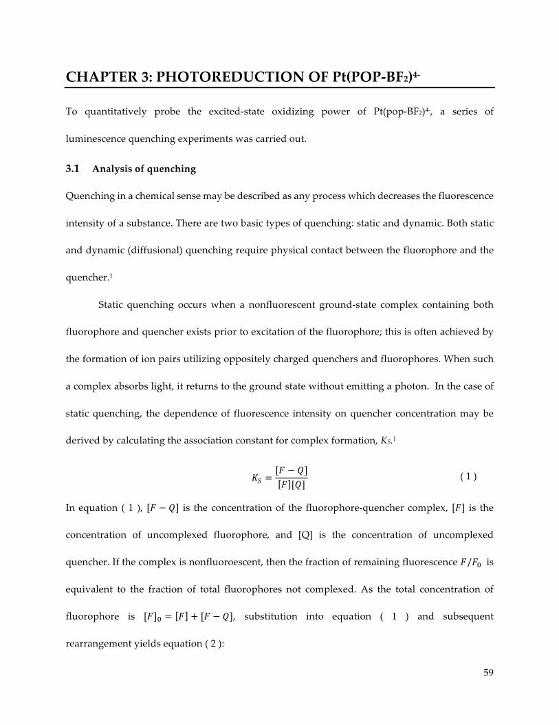
59
CHAPTER 3: PHOTOREDUCTION OF Pt(POP-BF2)4- To quantitatively probe the excited-state oxidizing power of Pt(pop-BF2)4-, a series of
luminescence quenching experiments was carried out.
3.1 Analysis of quenching
Quenching in a chemical sense may be described as any process which decreases the fluorescence
intensity of a substance. There are two basic types of quenching: static and dynamic. Both static
and dynamic (diffusional) quenching require physical contact between the fluorophore and the
quencher.1
Static quenching occurs when a nonfluorescent ground-state complex containing both
fluorophore and quencher exists prior to excitation of the fluorophore; this is often achieved by
the formation of ion pairs utilizing oppositely charged quenchers and fluorophores. When such
a complex absorbs light, it returns to the ground state without emitting a photon. In the case of
static quenching, the dependence of fluorescence intensity on quencher concentration may be
derived by calculating the association constant for complex formation, KS.1
𝐾" =[𝐹 − 𝑄]𝐹 [𝑄]
( 1 )
In equation ( 1 ), [𝐹 − 𝑄] is the concentration of the fluorophore-quencher complex, [𝐹] is the
concentration of uncomplexed fluorophore, and [Q] is the concentration of uncomplexed
quencher. If the complex is nonfluoroescent, then the fraction of remaining fluorescence 𝐹/𝐹* is
equivalent to the fraction of total fluorophores not complexed. As the total concentration of
fluorophore is [𝐹]* = 𝐹 + [𝐹 − 𝑄], substitution into equation ( 1 ) and subsequent
rearrangement yields equation ( 2 ):
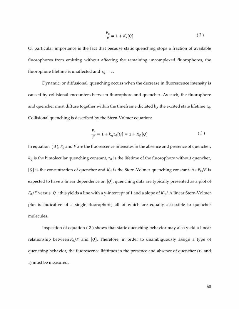
60
𝐹*𝐹= 1 + 𝐾.[𝑄] ( 2 )
Of particular importance is the fact that because static quenching stops a fraction of available
fluorophores from emitting without affecting the remaining uncomplexed fluorophores, the
fluorophore lifetime is unaffected and 𝜏* = 𝜏.
Dynamic, or diffusional, quenching occurs when the decrease in fluorescence intensity is
caused by collisional encounters between fluorophore and quencher. As such, the fluorophore
and quencher must diffuse together within the timeframe dictated by the excited state lifetime 𝜏*.
Collisional quenching is described by the Stern-Volmer equation:
𝐹*𝐹= 1 + 𝑘2𝜏* 𝑄 = 1 + 𝐾3[𝑄] ( 3 )
In equation ( 3 ), 𝐹* and 𝐹 are the fluorescence intensites in the absence and presence of quencher,
𝑘2 is the bimolecular quenching constant, 𝜏* is the lifetime of the fluorophore without quencher,
𝑄 is the concentration of quencher and 𝐾3 is the Stern-Volmer quenching constant. As 𝐹*/𝐹 is
expected to have a linear dependence on 𝑄 , quenching data are typically presented as a plot of
𝐹*/𝐹versus 𝑄 ; this yields a line with a y-intercept of 1 and a slope of 𝐾3.1 A linear Stern-Volmer
plot is indicative of a single fluorophore, all of which are equally accessible to quencher
molecules.
Inspection of equation ( 2 ) shows that static quenching behavior may also yield a linear
relationship between𝐹*/𝐹 and 𝑄 . Therefore, in order to unambiguously assign a type of
quenching behavior, the fluorescence lifetimes in the presence and absence of quencher (𝜏* and
𝜏) must be measured.

61
3.2 Fluorophore lifetime measurements
The excitation of a fluorophore with an infinitely short pulse of light results in an initial
population 𝑁* of fluorophores in the excited state. At any time 𝑡 after the initial excitation, the
number of excited molecules may be described as 𝑁(𝑡). As time passes, this population decays at
a rate dependent on the emissive rate 𝛾 and the non-radiative decay rate 𝑘9::
𝑑𝑁(𝑡)𝑑𝑡
= − 𝛾 + 𝑘9: 𝑁(𝑡) ( 4 )
As 𝑁 𝑡 = 0 = 𝑁*, equation ( 4 ) may be integrated to yield
𝑁 = 𝑁*𝑒>?/@ ( 5 )
in which 𝜏 is the lifetime of the excited state. The fluorescence lifetime is generally defined to be
the time required for the intensity to decay to 1/𝑒 of its original value; or,
𝜏 =1
𝛾 + 𝑘9: ( 6 )
Finally, the fluorescence intensity measured by an instrument, 𝐹(𝑡), is proportional to the excited
state population:
𝑁 𝑡 ≅ 𝐹(𝑡) ( 7 )
Thus, the slope of a plot of log𝐹(𝑡) versus 𝑡 will be −1/𝜏.
3.3 Quenching of 3[Pt(pop-BF2)4-]* phosphorescence
The excited-state lifetimes of the [Pt(pop-BF2)]4- singlet and triplet states were measured by
Durrell and coworkers in 2012. The triplet state has a lifetime of 8.4 𝜇s with an emission maximum
at 512 nm; meanwhile, the singlet state has a lifetime of 1.6 ns with an emission maximum of 393
nm.2 The length of the triplet lifetime affords ample time for diffusional quenching to occur. The

62
presence of diffusional quenching may be observed as a decrease in either luminescence lifetime
or steady-state luminescence intensity at the triplet emission wavelength maximum of 512 nm.
As shown in Figure 1, after the triplet excited state of Pt(pop-BF2)4- is produced following
excitation with 355 nm light, it may return to the ground state either by emission of a photon or
by reacting with an electron-transfer type quencher molecule to produce the oxidized quencher
and reduced Pt(pop-BF2)5-. The degree to which the nonemissive path is favored over the emissive
pathway is demonstrated by the relative magnitude of the decrease in luminescence intensity.
After quenching occurs, it is possible for the products to react to reform the reactants, Q and
Pt(pop-BF2)4-, provided that Q+ does not decompose.
Figure 1: Dynamic (diffusional) reductive quenching scheme.
The excited-state behavior of Pt(pop)4- is well known and has been deeply investigated,3-
12 while that of Pt(pop-BF2)4- remains relatively unexplored.13,14 Furthermore, as yet the only extant
data on the oxidizing power of Pt(pop-BF2)4- excited states are estimates based on spectral data
(see Chapter 1).2,13,15 By tracking how the quenching rate of an emissive state changes based on
the oxidation potential of the selected quencher molecule, a good estimate of the potential of the
excited state may be obtained.16-18 As such, the emissive properties of Pt(pop-BF2)4- were studied
in the presence of various organic amine quenchers. The specific amines used in this section were

63
chosen as quenchers because of their lack of absorption bands in the areas of Pt(pop-BF2)4-
absorption, their ranges of oxidation potential, and their solubility in acetonitrile.14
Briefly, solutions of Pt(pop-BF2)4- of a fixed concentration (~10 𝜇M) were prepared such
that the total absorbance at the 355 nm excitation wavelength was between 0.05 and 0.1; these
solutions were spiked with increasing concentrations of quencher and their steady-state
luminescence profiles were recorded using fluorimetry. Quencher-only solutions were also
prepared and analyzed to ensure that the quencher was not luminescing due to excitation from
the 355 nm probe wavelength. The singlet emission intensity was measured and used as a
normalization factor, as the 1.6 ns lifetime of the singlet state hampers it from participating in
diffusional quenching; furthermore, noted deviation in the singlet-state intensity from spectrum
to spectrum was within instrument error.2 Finally, the solutions were monitored by UV-Vis
spectroscopy during the course of the experiment to check for any possible decomposition; no
such decomposition was observed. Stern-Volmer type quenching behavior was observed, and
values for kq were calculated for each quencher by plotting I0/I (referred to as F0/F in the equations
of section 3.1) vs [Q]. Results are summarized in Figure 2, Figure 3, and Figure 4.
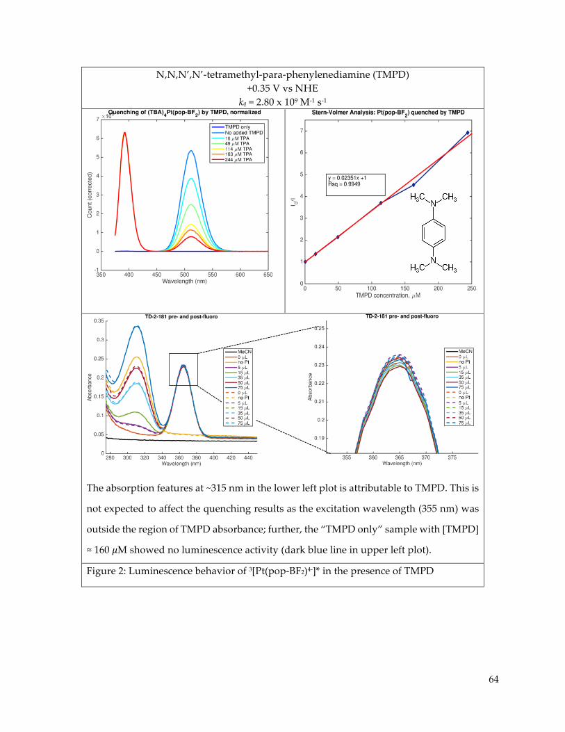
64
N,N,N’,N’-tetramethyl-para-phenylenediamine (TMPD) +0.35 V vs NHE
kq = 2.80 x 10⁹ M-1 s-1
The absorption features at ~315 nm in the lower left plot is attributable to TMPD. This is
not expected to affect the quenching results as the excitation wavelength (355 nm) was
outside the region of TMPD absorbance; further, the “TMPD only” sample with [TMPD]
≈ 160 𝜇M showed no luminescence activity (dark blue line in upper left plot).
Figure 2: Luminescence behavior of 3[Pt(pop-BF2)4-]* in the presence of TMPD
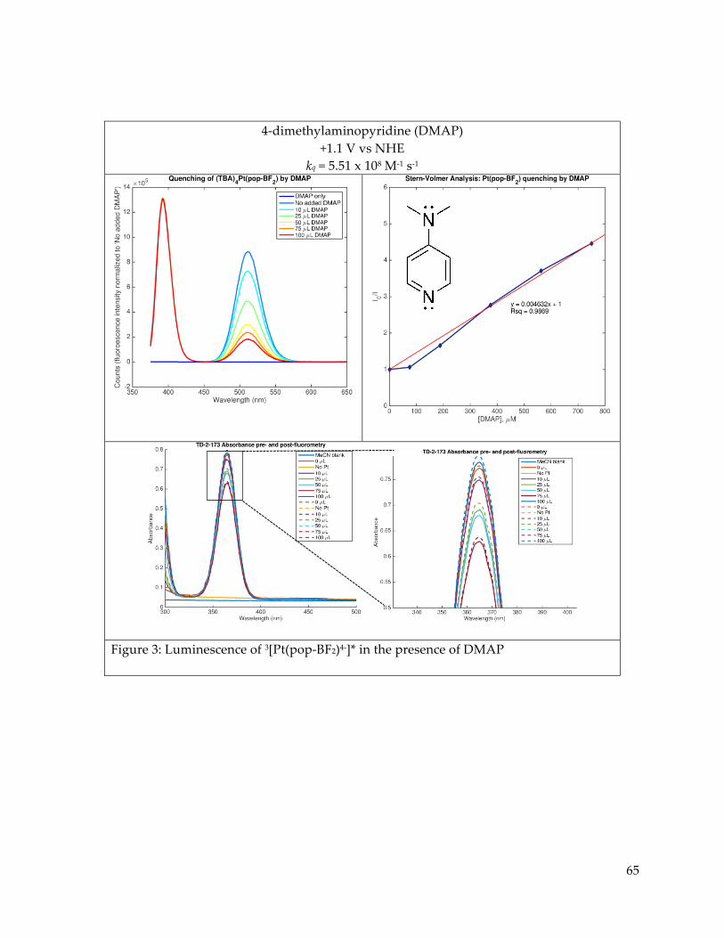
65
4-dimethylaminopyridine (DMAP) +1.1 V vs NHE
kq = 5.51 x 10⁸ M-1 s-1
Figure 3: Luminescence of 3[Pt(pop-BF2)4-]* in the presence of DMAP
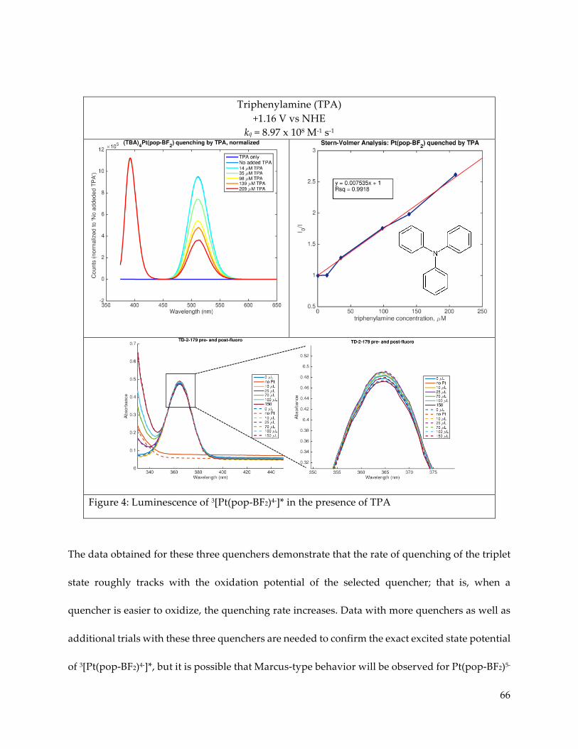
66
Triphenylamine (TPA) +1.16 V vs NHE
kq = 8.97 x 10⁸ M-1 s-1
Figure 4: Luminescence of 3[Pt(pop-BF2)4-]* in the presence of TPA
The data obtained for these three quenchers demonstrate that the rate of quenching of the triplet
state roughly tracks with the oxidation potential of the selected quencher; that is, when a
quencher is easier to oxidize, the quenching rate increases. Data with more quenchers as well as
additional trials with these three quenchers are needed to confirm the exact excited state potential
of 3[Pt(pop-BF2)4-]*, but it is possible that Marcus-type behavior will be observed for Pt(pop-BF2)5-
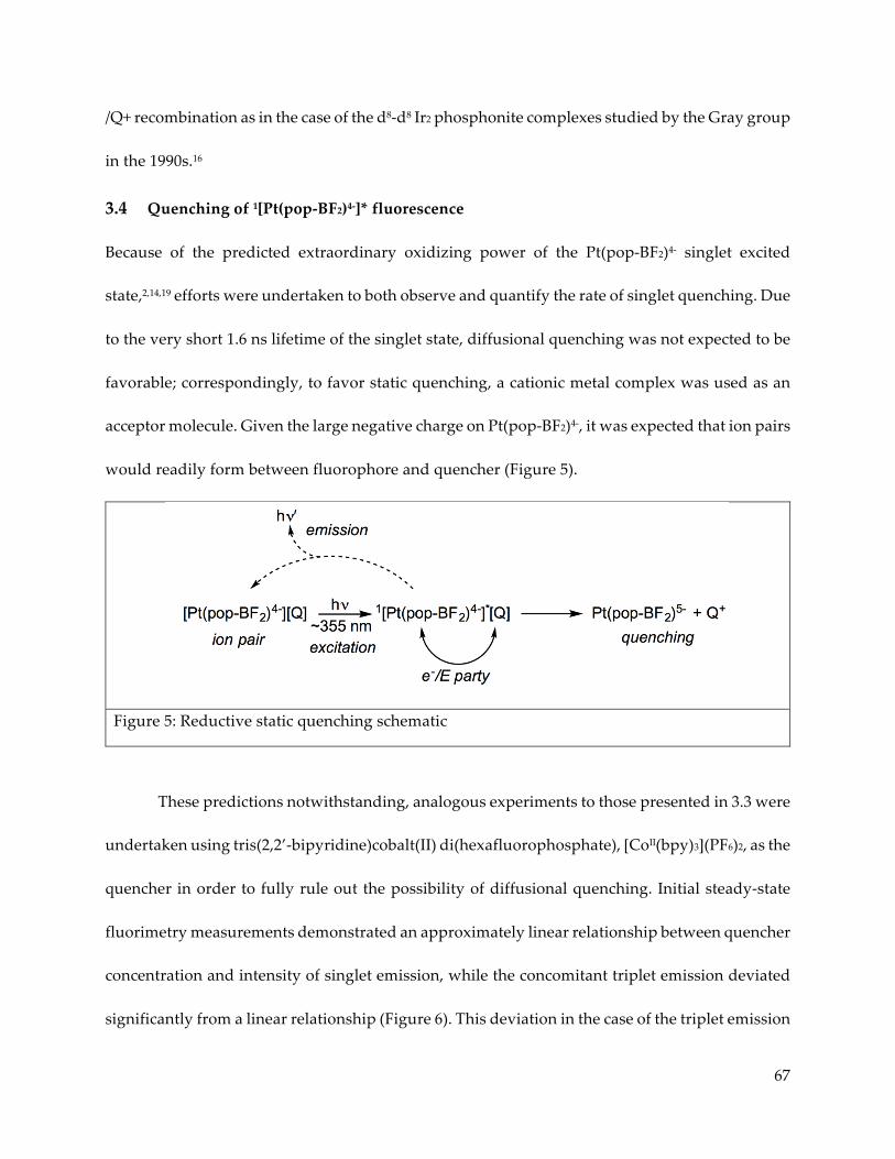
67
/Q+ recombination as in the case of the d8-d8 Ir2 phosphonite complexes studied by the Gray group
in the 1990s.16
3.4 Quenching of 1[Pt(pop-BF2)4-]* fluorescence
Because of the predicted extraordinary oxidizing power of the Pt(pop-BF2)4- singlet excited
state,2,14,19 efforts were undertaken to both observe and quantify the rate of singlet quenching. Due
to the very short 1.6 ns lifetime of the singlet state, diffusional quenching was not expected to be
favorable; correspondingly, to favor static quenching, a cationic metal complex was used as an
acceptor molecule. Given the large negative charge on Pt(pop-BF2)4-, it was expected that ion pairs
would readily form between fluorophore and quencher (Figure 5).
Figure 5: Reductive static quenching schematic
These predictions notwithstanding, analogous experiments to those presented in 3.3 were
undertaken using tris(2,2’-bipyridine)cobalt(II) di(hexafluorophosphate), [CoII(bpy)3](PF6)2, as the
quencher in order to fully rule out the possibility of diffusional quenching. Initial steady-state
fluorimetry measurements demonstrated an approximately linear relationship between quencher
concentration and intensity of singlet emission, while the concomitant triplet emission deviated
significantly from a linear relationship (Figure 6). This deviation in the case of the triplet emission
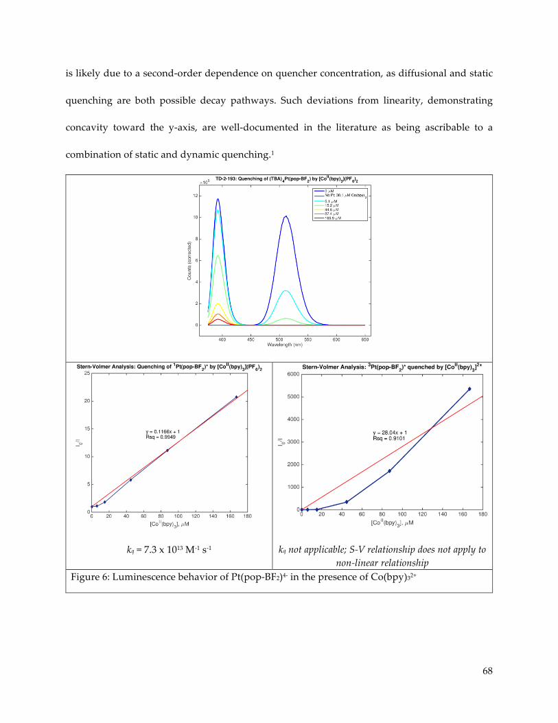
68
is likely due to a second-order dependence on quencher concentration, as diffusional and static
quenching are both possible decay pathways. Such deviations from linearity, demonstrating
concavity toward the y-axis, are well-documented in the literature as being ascribable to a
combination of static and dynamic quenching.1
kq = 7.3 x 10¹³ M-1 s-1
kq not applicable; S-V relationship does not apply to non-linear relationship
Figure 6: Luminescence behavior of Pt(pop-BF2)4- in the presence of Co(bpy)32+

69
A putative singlet quenching rate exceeding 1013 M-1 s-1 was also calculated, seemingly
ruling out the possibility of a wholly diffusional quenching mechanism given that the diffusion
limit in acetonitrile is on the order of 1011 M-1 s-1. However, close investigation of the plot of I0/I vs
[Q] indicates a very slight
deviation from linearity at
lower concentrations. A
possible explanation for this
deviation could be that at low
[Q] there is little to no
quenching, as the singlet
lifetime is too short to allow for
diffusional quenching and [Q]
could be too low to create a
sizable population of quencher-
fluorophore complexes. Contrastingly, at high [Q], rapid quenching (i.e. quenching rates in excess
of the diffusion limit) could be attributed to static quenching behavior resulting from the favored
formation of quencher-fluorophore complexes (Figure 7).
In an effort to further illuminate this behavior, quencher concentrations were lowered to
<20 𝜇M to attempt to disfavor fluorophore-quencher complex formation and to add more data
points to the plot in Figure 7. However, with the additional data at lower concentrations, the
deviation from linearity was even more distinct for both the singlet and triplet states (Figure 8).
Figure 7: Indication of possible bimodal quenching behavior
Complex formation at higher[Co] could explain rapidquenching
At lower concentrations, little
tonoquenching?

70
Figure 8: Substantial quenching of Pt(pop-BF2)4- singlet and triplet emission continues at low values of [Q]
Furthermore, the additional data points taken at lower concentrations follow the same pattern
observed previously (Figure 9).
Figure 9: Overlay of quenching data obtained with [Q] = 0 – 170 𝜇M (yellow) and [Q] = 0 – 20 𝜇M (blue).
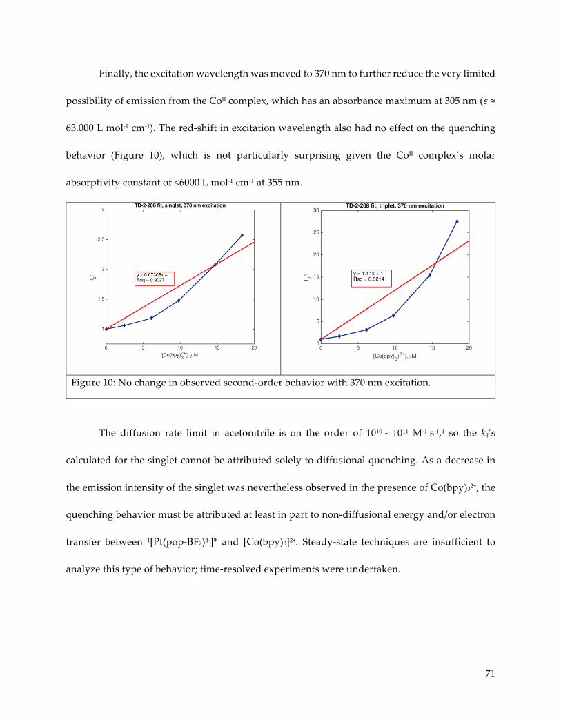
71
Finally, the excitation wavelength was moved to 370 nm to further reduce the very limited
possibility of emission from the CoII complex, which has an absorbance maximum at 305 nm (𝜖 ≈
63,000 L mol-1 cm-1). The red-shift in excitation wavelength also had no effect on the quenching
behavior (Figure 10), which is not particularly surprising given the CoII complex’s molar
absorptivity constant of <6000 L mol-1 cm-1 at 355 nm.
Figure 10: No change in observed second-order behavior with 370 nm excitation.
The diffusion rate limit in acetonitrile is on the order of 1010 - 1011 M-1 s-1,1 so the kq’s
calculated for the singlet cannot be attributed solely to diffusional quenching. As a decrease in
the emission intensity of the singlet was nevertheless observed in the presence of Co(bpy)32+, the
quenching behavior must be attributed at least in part to non-diffusional energy and/or electron
transfer between 1[Pt(pop-BF2)4-]* and [Co(bpy)3]2+. Steady-state techniques are insufficient to
analyze this type of behavior; time-resolved experiments were undertaken.
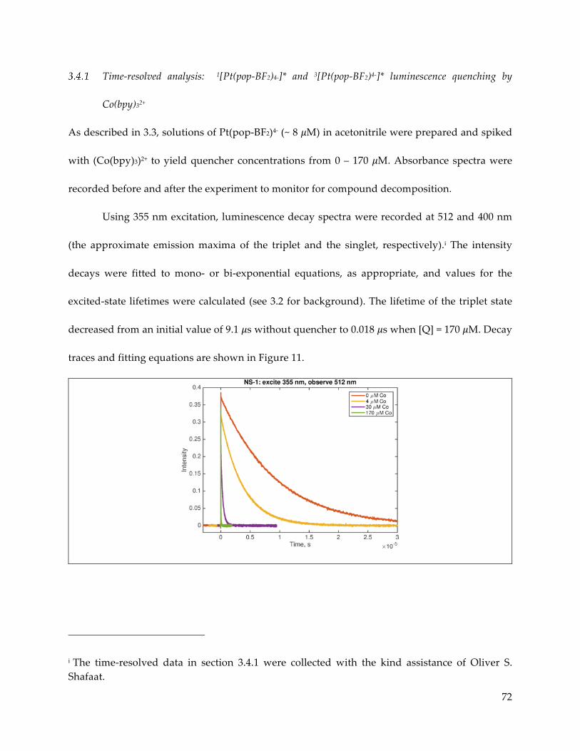
72
Time-resolved analysis: 1[Pt(pop-BF2)4-]* and 3[Pt(pop-BF2)4-]* luminescence quenching by
Co(bpy)32+
As described in 3.3, solutions of Pt(pop-BF2)4- (~ 8 𝜇M) in acetonitrile were prepared and spiked
with (Co(bpy)3)2+ to yield quencher concentrations from 0 – 170 𝜇M. Absorbance spectra were
recorded before and after the experiment to monitor for compound decomposition.
Using 355 nm excitation, luminescence decay spectra were recorded at 512 and 400 nm
(the approximate emission maxima of the triplet and the singlet, respectively).i The intensity
decays were fitted to mono- or bi-exponential equations, as appropriate, and values for the
excited-state lifetimes were calculated (see 3.2 for background). The lifetime of the triplet state
decreased from an initial value of 9.1 𝜇s without quencher to 0.018 𝜇s when [Q] = 170 𝜇M. Decay
traces and fitting equations are shown in Figure 11.
i The time-resolved data in section 3.4.1 were collected with the kind assistance of Oliver S. Shafaat.
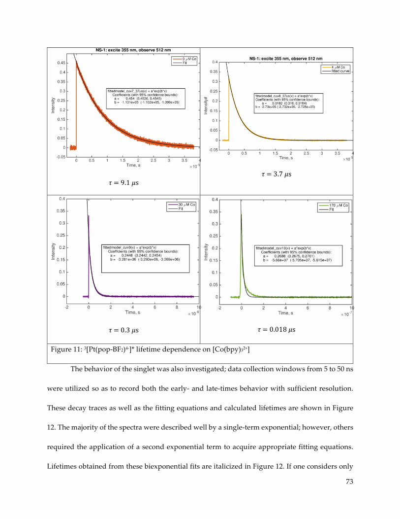
73
𝜏=9.1𝜇s
𝜏=3.7𝜇s
𝜏=0.3𝜇s
𝜏=0.018𝜇s
Figure 11: 3[Pt(pop-BF2)4-]* lifetime dependence on [Co(bpy)32+]
The behavior of the singlet was also investigated; data collection windows from 5 to 50 ns
were utilized so as to record both the early- and late-times behavior with sufficient resolution.
These decay traces as well as the fitting equations and calculated lifetimes are shown in Figure
12. The majority of the spectra were described well by a single-term exponential; however, others
required the application of a second exponential term to acquire appropriate fitting equations.
Lifetimes obtained from these biexponential fits are italicized in Figure 12. If one considers only

74
the data sets which could be reasonably described by a simple exponential decay, the lifetime for
1[Pt(pop-BF2)4-]* with 4 𝜇M [Co(bpy)32+] was nearly identical (𝜏 ≈ 1.65 – 1.73 ns) to the unquenched
𝜏0 value of 1.67 – 1.70 ns. When [Co(bpy)32+] increased to 30 𝜇M, the singlet lifetime decreased
measurably to ≈ 1.55 ns. If the only quenching mechanism in action is static quenching, 𝜏 should
equal 𝜏0. A possible explanation is that for [Co(bpy)32+] ≲ 30 𝜇M, only static quenching is at work.
When [Co(bpy)32+] increases beyond that, complex formation may no longer be favored as
proscribed by 𝐾", equation ( 1 ). This could occur, for instance, if [Co(bpy)32+] ≫ [Pt(pop-BF2)4-]. If
complex formation is not favored and uncomplexed quencher still remains in solution, that excess
quencher could facilitate diffusional quenching.
While it is unlikely that quencher and fluorophore could diffuse over long distances in
the span of less than two nanoseconds, it is possible to have quencher and fluorophore close
enough to each other at the time of excitation to cause near-instantaneous quenching.1 This
“sphere of action”-type behavior implicates a more complex quenching mechanism involving
different degrees of static and diffusional quenching depending on the quencher concentration.
To fully deconvolute the behavior, more data are needed; a potential analytical scheme is
presented in section 3.5. Repeating the experiments described in this section with a broader range
of quencher concentrations would provide needed information about exactly when 𝜏 begins to
deviate from 𝜏0. Furthermore, investigating the effects of temperature and solvent choice on the
fluorophore-quencher interaction would allow the use of more accurate calculations that account
for diffusional and static quenching behavior simultaneously.1
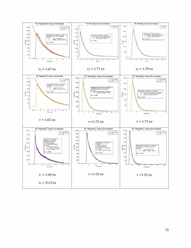
75
𝜏0=1.67ns
𝜏0=1.71ns
𝜏0=1.70ns
𝜏=1.65ns
𝜏=1.72ns
𝜏=1.73ns
𝜏a=1.60ns
𝜏b=0.13ns
𝜏=1.53ns
𝜏=1.52ns

76
𝜏a=1.41ns
𝜏b=0.12ns
𝜏a=1.94ns
𝜏b=0.22ns
𝜏=0.82ns
Figure 12: 1[Pt(pop-BF2)4-]* lifetime dependence on [Co(bpy)2+]
Another possible contributing factor to the somewhat puzzling luminescence behavior is
sample decomposition, which was unfortunately noted over the course of these laser experiments
(Figure 13). The right-hand plot in Figure 13 shows the absorption maximum of Pt(pop-BF2)4-;
decreases in absorption intensity are noted for all samples over the course of the experiment. The
full trace on the left additionally shows significant changes in absorption below 300 nm, where
bands for both Pt(pop-BF2)4- and Co(bpy)2+ typically present. The composition of the samples
undoubtedly changed during the experiment; the effects of those changes on the luminescence
properties are unknown.
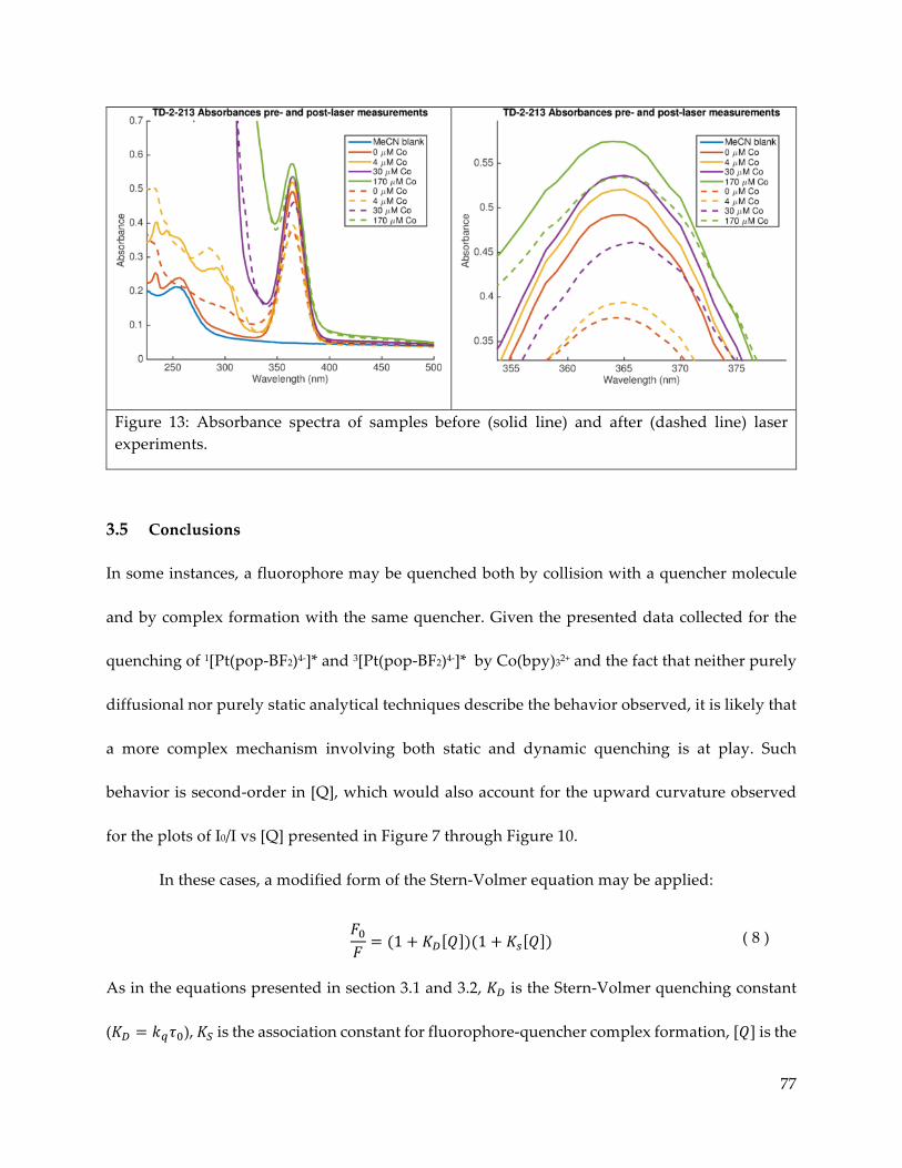
77
Figure 13: Absorbance spectra of samples before (solid line) and after (dashed line) laser experiments.
3.5 Conclusions
In some instances, a fluorophore may be quenched both by collision with a quencher molecule
and by complex formation with the same quencher. Given the presented data collected for the
quenching of 1[Pt(pop-BF2)4-]* and 3[Pt(pop-BF2)4-]* by Co(bpy)32+ and the fact that neither purely
diffusional nor purely static analytical techniques describe the behavior observed, it is likely that
a more complex mechanism involving both static and dynamic quenching is at play. Such
behavior is second-order in [Q], which would also account for the upward curvature observed
for the plots of I0/I vs [Q] presented in Figure 7 through Figure 10.
In these cases, a modified form of the Stern-Volmer equation may be applied:
𝐹*𝐹= (1 + 𝐾3 𝑄 )(1 + 𝐾. 𝑄 ) ( 8 )
As in the equations presented in section 3.1 and 3.2, 𝐾3 is the Stern-Volmer quenching constant
(𝐾3 = 𝑘2𝜏*), 𝐾" is the association constant for fluorophore-quencher complex formation, [𝑄] is the

78
concentration of quencher, and 𝐹*/𝐹 is the ratio of unquenched luminescence intensity to the
observed luminescence intensity at any quencher concentration [𝑄]. The dynamic part of the
observed quenching may be determined via lifetime measurements:
𝜏*𝜏= 1 + 𝐾3[𝑄] ( 9 )
Combination of equations ( 8 ) and ( 9 ) yields the following relation:
𝐹*𝐹=
𝜏*𝜏[T]
(1 + 𝐾" 𝑄 ) ( 10 )
The analysis put forward in equation ( 10 ) requires a complete set of steady-state and time-
resolved quenching data for a single set of samples; lifetimes and steady-state intensities must be
acquired that the exact same concentrations of 𝑄. Given the decomposition issues consistently
observed with Pt(pop-BF2)4- over the course of time-resolved laser experiments, a complete set of
data is not available at this time. That said, Pt(pop-BF2)4- in the presence of amine-type quenchers
(as presented in section 3.3) exhibits classic Stern-Volmer-type dynamic quenching behavior of
the triplet state. Additional research in this area could lend valuable insight to the mechanism of
combined static and dynamic quenching of both the singlet and triplet states of Pt(pop-BF2)4- in
the presence of metal complexes like Co(bpy)32+.
3.6 Materials and methods
Unless otherwise noted, all reagents were obtained from Sigma-Aldrich and used without further
purification; all water used was deionized. All manipulations involving Pt(pop-BF2)4- were
carried out with standard air-free techniques in an inert-atmosphere glovebox or utilizing a
vacuum manifold. Solvents were dried using activated alumina columns according to Grubbs’

79
method.20 Anhydrous acetonitrile was stored over activated 3 Å molecular sieves; all other
anhydrous solvents were stored over activated 4 Å molecular sieves.21 Molecular sieves were
activated by heating to 200 ºC under reduced pressure for 4 hours.
[Co(bpy)3](PF6)2 22,23
Co(bpy)3Cl2 was formed by mixing a solution of 3.27 g 2,2’-bipyridine in 100 mL methanol with
a solution of 1.66 CoCl2•6H2O in 50 mL methanol and stirring for one hour. 11.4 g NH4PF6 was
added to precipitate 8.3 g of a light yellow solid. This product was dissolved in 150 mL CH2Cl2
and filtered to remove ~ 2g residual NH4Cl and NH4PF6 as a yellowish-white powder. The mother
liquor was reduced in volume via rotary evaporation to yield shiny orange microcrystalline
needles, which were rinsed with diethyl ether and dried under vacuum. Further purification may
be achieved by recrystallization from acetone/methanol.
Steady-state quenching experiments
Steady-state emission spectra were recorded on a Jobin Yvon Spex Fluorolog-3-11. A 450-W xenon
arc lamp was used as the excitation source with a single monochromator providing wavelength
selection. Right-angle light emission was sorted using a single monochromator and fed into a
Hamamatsu R928P photomultiplier tube with photon counting. Short and long pass filters were
used where appropriate. Spectra were recorded on Datamax software.2

80
Time-resolved quenching experiments
To monitor singlet and triplet emission, samples were excited at 355 nm with 8-ns pulses from
the third harmonic of a Q- switched Nd:YAG laser (Spectra-Physics Quanta-Ray PRO-Series)
operating at 10 Hz. Emission wavelengths were selected using a double monochromator
(Instruments SA DH-10) with 1 mm slits. Luminescence was detected with a photomultiplier tube
(PMT, Hamamatsu R928). The PMT current was amplified and recorded with a transient digitizer
(Tektronix DSA 602). Short- and long-pass filters were employed to remove scattered excitation
light. Decay traces were averaged over 500 laser pulses. Instruments and electronics in this system
were controlled by software written in LabVIEW (National Instruments). Data manipulation was
performed and plotted using MATLAB R2015a (Mathworks, Inc.).2
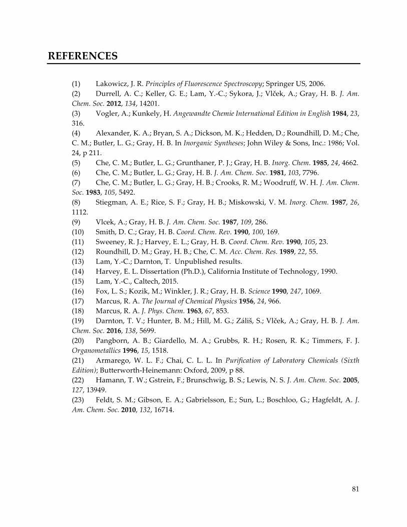
81
REFERENCES (1) Lakowicz, J. R. Principles of Fluorescence Spectroscopy; Springer US, 2006. (2) Durrell, A. C.; Keller, G. E.; Lam, Y.-C.; Sykora, J.; Vlček, A.; Gray, H. B. J. Am.
Chem. Soc. 2012, 134, 14201. (3) Vogler, A.; Kunkely, H. Angewandte Chemie International Edition in English 1984, 23,
316. (4) Alexander, K. A.; Bryan, S. A.; Dickson, M. K.; Hedden, D.; Roundhill, D. M.; Che,
C. M.; Butler, L. G.; Gray, H. B. In Inorganic Syntheses; John Wiley & Sons, Inc.: 1986; Vol. 24, p 211.
(5) Che, C. M.; Butler, L. G.; Grunthaner, P. J.; Gray, H. B. Inorg. Chem. 1985, 24, 4662. (6) Che, C. M.; Butler, L. G.; Gray, H. B. J. Am. Chem. Soc. 1981, 103, 7796. (7) Che, C. M.; Butler, L. G.; Gray, H. B.; Crooks, R. M.; Woodruff, W. H. J. Am. Chem.
Soc. 1983, 105, 5492. (8) Stiegman, A. E.; Rice, S. F.; Gray, H. B.; Miskowski, V. M. Inorg. Chem. 1987, 26,
1112. (9) Vlcek, A.; Gray, H. B. J. Am. Chem. Soc. 1987, 109, 286. (10) Smith, D. C.; Gray, H. B. Coord. Chem. Rev. 1990, 100, 169. (11) Sweeney, R. J.; Harvey, E. L.; Gray, H. B. Coord. Chem. Rev. 1990, 105, 23. (12) Roundhill, D. M.; Gray, H. B.; Che, C. M. Acc. Chem. Res. 1989, 22, 55. (13) Lam, Y.-C.; Darnton, T. Unpublished results. (14) Harvey, E. L. Dissertation (Ph.D.), California Institute of Technology, 1990. (15) Lam, Y.-C., Caltech, 2015. (16) Fox, L. S.; Kozik, M.; Winkler, J. R.; Gray, H. B. Science 1990, 247, 1069. (17) Marcus, R. A. The Journal of Chemical Physics 1956, 24, 966. (18) Marcus, R. A. J. Phys. Chem. 1963, 67, 853. (19) Darnton, T. V.; Hunter, B. M.; Hill, M. G.; Záliš, S.; Vlček, A.; Gray, H. B. J. Am.
Chem. Soc. 2016, 138, 5699. (20) Pangborn, A. B.; Giardello, M. A.; Grubbs, R. H.; Rosen, R. K.; Timmers, F. J.
Organometallics 1996, 15, 1518. (21) Armarego, W. L. F.; Chai, C. L. L. In Purification of Laboratory Chemicals (Sixth
Edition); Butterworth-Heinemann: Oxford, 2009, p 88. (22) Hamann, T. W.; Gstrein, F.; Brunschwig, B. S.; Lewis, N. S. J. Am. Chem. Soc. 2005,
127, 13949. (23) Feldt, S. M.; Gibson, E. A.; Gabrielsson, E.; Sun, L.; Boschloo, G.; Hagfeldt, A. J.
Am. Chem. Soc. 2010, 132, 16714.

82
CHAPTER 4: PREPARATION AND CHARACTERIZATION OF Pt(POP-BF2)5- AND Pt(POP-BF2)6- Extensive studies of Pt(pop)4- have demonstrated that optical excitation of an electron populates
a p𝜎 orbital with bonding character1, which strengthens the Pt-Pt interaction and causes a
shortening of the Pt-Pt distance by 0.21-0.31 Å as determined by both X-ray and optical
techniques.2-4 Theoretical work performed by Lam in collaboration with Vlček and Záliš predicted
an analogous bond shortening of 0.18 Å in Pt(pop-BF2)4-.5 As in optical excitation, direct reduction
of Pt(pop-BF2)4- was expected to fill the p𝜎 orbital, forming a weak Pt-Pt bond. While reversible
electrochemical reduction of the parent compound Pt(pop)4- has never been reported, Pt(pop)5-
has nevertheless been generated via pulse radiolysis in aqueous solution.6,7 Given the lack of
easily reduced –O—H···O— groups in Pt(pop-BF2)4-, reversible reduction seemed likely, and
electrochemical studies were undertaken.
4.1 Electrochemical reductions
Pt(pop-BF2)4- in acetonitrile (MeCN) undergoes one-electron reductions at E1/2 = -1.68 V and Ep =
-2.46 V vs Fc+/Fc (Figure 1).i The first wave is chemically reversible and electrochemically
quasireversible at a scan rate of 50 mV/s, as shown by the 𝛥Ep= 155 mV for the wave of interest
vs ~100 mV for Fc+/Fc under very similar conditions. The second wave is electrochemically
irreversible and chemically reversible, indicating formation of a superreduced complex Pt(pop-
BF2)6- which is stable at least at 273 K (see 4.2). Scanning anodically, a 2-electron chemically
i Electro- and spectroelectrochemical data were collected in collaboration with Bryan M. Hunter and Michael G. Hill.

83
irreversible oxidation is observed at +0.94 V vs Fc+/Fc. The full-range cyclic voltammogram is
shown in Figure 2.
Figure 1: Cyclic voltammogram of Pt(pop-BF2)4- in MeCN containing 0.1 M tetrabutylammonium hexafluorophosphate (Bu4NPF6) at 273 K. Potentials vs Fc+/Fc; scan rate of 50 mV/s.
Figure 2: Full-range cyclic voltammogram of Pt(pop-BF2)4- in MeCN containing 0.1 M (Bu4NPF6) at 273 K. Potentials vs Fc+/Fc; scan rate of 200 mV/s.
The first reduction of Pt(pop)4- has been estimated from reductive quenching kinetics to
be approximately -1.8 V, as compared to the -1.68 V obtained for Pt(pop-BF2)4-.8 This difference in
potentials is likely attributable to the strong electron-withdrawing effects of the BF2 groups,
which may be transmitted to the metal atoms by delocalization of the p𝜎 orbital over the
phosphorous atoms acting as donors to the Pt-Pt unit.9
Furthermore, potentials for the excited state redox couples can be estimated at 1.57 V for
1[Pt(pop-BF2)4-/5-]* and 0.86 V for 3[Pt(pop-BF2)4-/5-]* (both versus Fc+/Fc) using spectroscopically
determined excited-state energies;10 continuation of the work described in Chapter 3 could offer
further insight into these values.
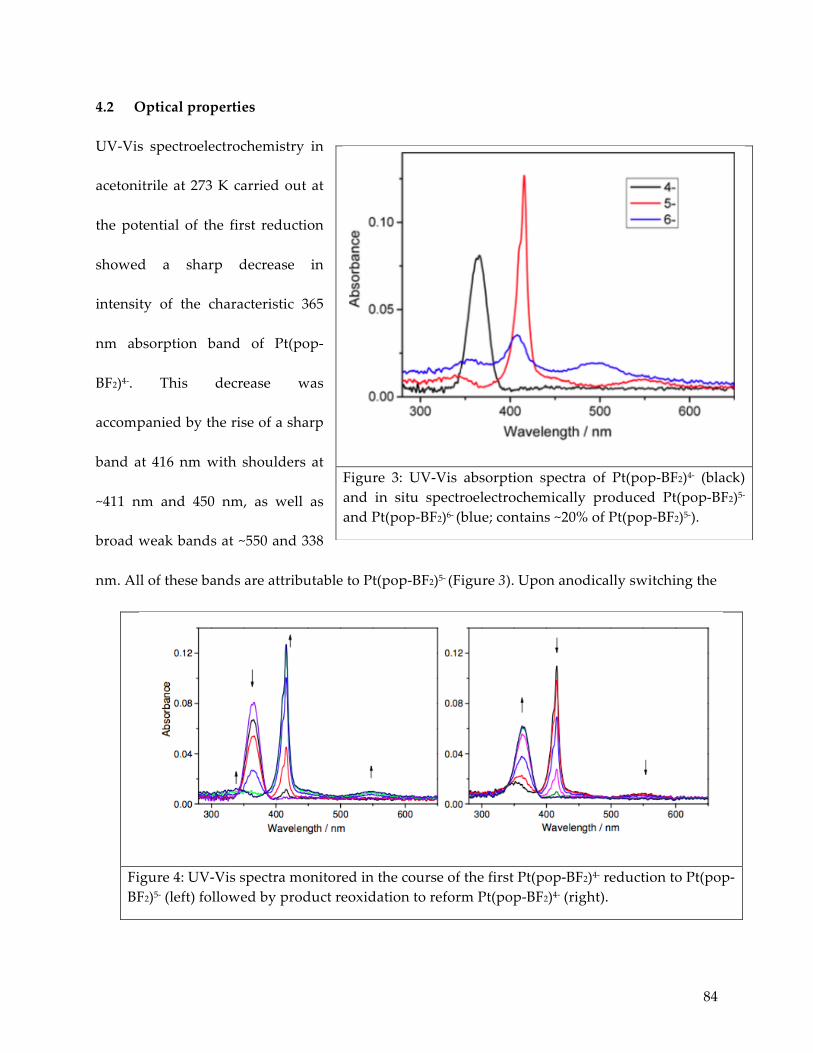
84
4.2 Optical properties
UV-Vis spectroelectrochemistry in
acetonitrile at 273 K carried out at
the potential of the first reduction
showed a sharp decrease in
intensity of the characteristic 365
nm absorption band of Pt(pop-
BF2)4-. This decrease was
accompanied by the rise of a sharp
band at 416 nm with shoulders at
~411 nm and 450 nm, as well as
broad weak bands at ~550 and 338
nm. All of these bands are attributable to Pt(pop-BF2)5- (Figure 3). Upon anodically switching the
Figure 3: UV-Vis absorption spectra of Pt(pop-BF2)4- (black) and in situ spectroelectrochemically produced Pt(pop-BF2)5- and Pt(pop-BF2)6- (blue; contains ~20% of Pt(pop-BF2)5-).
Figure 4: UV-Vis spectra monitored in the course of the first Pt(pop-BF2)4- reduction to Pt(pop-BF2)5- (left) followed by product reoxidation to reform Pt(pop-BF2)4- (right).
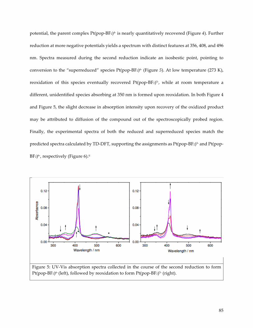
85
potential, the parent complex Pt(pop-BF2)4- is nearly quantitatively recovered (Figure 4). Further
reduction at more negative potentials yields a spectrum with distinct features at 356, 408, and 496
nm. Spectra measured during the second reduction indicate an isosbestic point, pointing to
conversion to the “superreduced” species Pt(pop-BF2)6- (Figure 5). At low temperature (273 K),
reoxidation of this species eventually recovered Pt(pop-BF2)5-, while at room temperature a
different, unidentified species absorbing at 350 nm is formed upon reoxidation. In both Figure 4
and Figure 5, the slight decrease in absorption intensity upon recovery of the oxidized product
may be attributed to diffusion of the compound out of the spectroscopically probed region.
Finally, the experimental spectra of both the reduced and superreduced species match the
predicted spectra calculated by TD-DFT, supporting the assignments as Pt(pop-BF2)5- and Pt(pop-
BF2)6-, respectively (Figure 6).ii
Figure 5: UV-Vis absorption spectra collected in the course of the second reduction to form Pt(pop-BF2)6- (left), followed by reoxidation to form Pt(pop-BF2)5- (right).

86
Figure 6: TD-DFT simulated UV-vis absorption spectra of Pt(pop-BF2)n– (n = 4 (black), 5 (red) and 6 (blue). The same FWHM of 3000 cm–1 was assumed for all transitions. TD- DFT (PBE0/PCM-MeCN).ii
ii Theoretical simulations contributed by S. Záliš and A. Vlček.
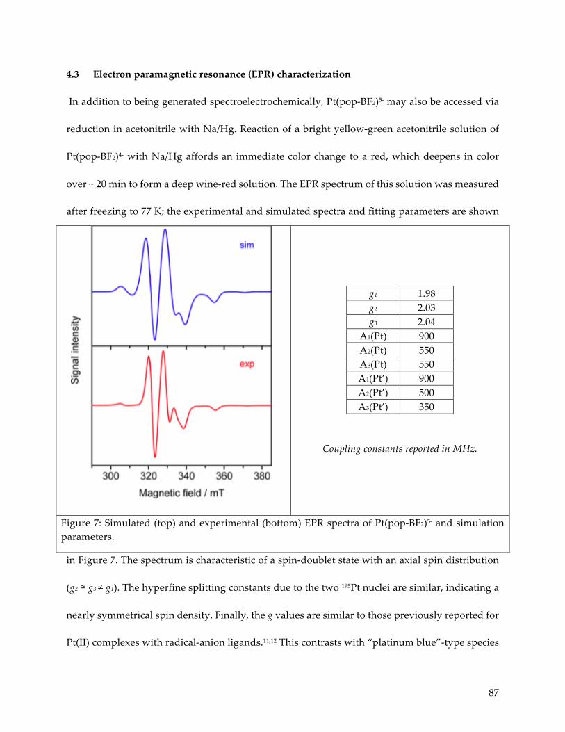
87
4.3 Electron paramagnetic resonance (EPR) characterization
In addition to being generated spectroelectrochemically, Pt(pop-BF2)5- may also be accessed via
reduction in acetonitrile with Na/Hg. Reaction of a bright yellow-green acetonitrile solution of
Pt(pop-BF2)4- with Na/Hg affords an immediate color change to a red, which deepens in color
over ~ 20 min to form a deep wine-red solution. The EPR spectrum of this solution was measured
after freezing to 77 K; the experimental and simulated spectra and fitting parameters are shown
in Figure 7. The spectrum is characteristic of a spin-doublet state with an axial spin distribution
(g2 ≅ g3 ≠ g1). The hyperfine splitting constants due to the two 195Pt nuclei are similar, indicating a
nearly symmetrical spin density. Finally, the g values are similar to those previously reported for
Pt(II) complexes with radical-anion ligands.11,12 This contrasts with “platinum blue”-type species
g1 1.98 g2 2.03 g3 2.04
A1(Pt) 900 A2(Pt) 550 A3(Pt) 550 A1(Pt’) 900 A2(Pt’) 500 A3(Pt’) 350
Coupling constants reported in MHz.
Figure 7: Simulated (top) and experimental (bottom) EPR spectra of Pt(pop-BF2)5- and simulation parameters.
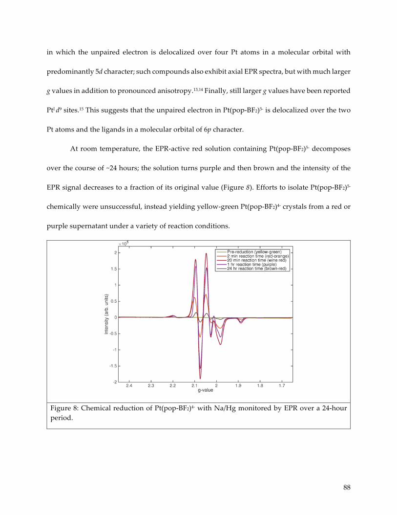
88
in which the unpaired electron is delocalized over four Pt atoms in a molecular orbital with
predominantly 5d character; such compounds also exhibit axial EPR spectra, but with much larger
g values in addition to pronounced anisotropy.13,14 Finally, still larger g values have been reported
PtI d9 sites.15 This suggests that the unpaired electron in Pt(pop-BF2)5- is delocalized over the two
Pt atoms and the ligands in a molecular orbital of 6p character.
At room temperature, the EPR-active red solution containing Pt(pop-BF2)5- decomposes
over the course of ~24 hours; the solution turns purple and then brown and the intensity of the
EPR signal decreases to a fraction of its original value (Figure 8). Efforts to isolate Pt(pop-BF2)5-
chemically were unsuccessful, instead yielding yellow-green Pt(pop-BF2)4- crystals from a red or
purple supernatant under a variety of reaction conditions.
Figure 8: Chemical reduction of Pt(pop-BF2)4- with Na/Hg monitored by EPR over a 24-hour period.

89
4.4 Electronic structures
The spectroscopic changes recorded in the course of the reduction together with DFT calculations
point to successive filling of the pσ molecular orbital. The strong, sharp dσ*⟶pσ band is the
lowest-energy feature in the spectrum of the parent complex. It also is present in the reduced (5-
) species with a (dσ*)2(pσ)1 configuration, but it is preceded in energy by a weaker band
attributable to pσ excitation. The UV−vis spectral pattern changes completely in the superreduced
complex, as the pσ orbital becomes fully occupied. The dσ*⟶pσ transition vanishes, and the
spectrum exhibits a series of transitions from the pσ HOMO to higher unoccupied orbitals.
Successive filling of the pσ orbital formally generates a Pt−Pt σ bond without changing
the Pt 5d8 electronic configuration, making Pt(pop-BF2)6− a very rare 6p2 σ-bonded binuclear
complex. The DFT-calculated Mayer−Mulliken bond ordersiii show strengthening of the Pt−Pt
bonding interaction upon reduction, whereby the bond order increases about 2-fold on going
from the 4− parent (0.17) to the 6− superreduced complex (0.34).9 While significant, the Pt−Pt
bonding in Pt(pop-BF2)6− is far from a full σ-bond, as the Pt−Pt bonding interaction is limited by
several structural and electronic factors. The rigid pop-BF2 ligand cage does not allow the
metal−metal distance to shorten very much, disfavoring effective orbital overlap; the
(5dσ)2(5dσ*)2(6pσ)2 configuration places six σ electrons in spatial proximity with one another,
producing repulsive electronic congestion along the Pt−Pt axis; and the pσ molecular orbital is
only 59% 6pz in character, being delocalized over the Pt−P bonds. Accordingly, Pt−P bond orders
iii Theoretical simulations contributed by S. Záliš and A. Vlček; further details available in reference 9.

90
also gradually increase upon reduction. The EPR spectrum of Pt(pop-BF2)5− confirms the
delocalized nature of the singly occupied 6pσ molecular orbital, showing axial spin density
distribution (see section 4.3).
The Pt−Pt distance was calculated to shorten by 0.08 and 0.06 Å upon the first and second
reductions, respectively, while the calculated Pt−Pt stretching frequency ν(Pt−Pt) increases from
128 cm−1 in the parent complex to 146 (5−) and 170 cm−1 (6−).9 The reduced species essentially
keeps the high symmetry of the parent complex, which is manifested both by the calculation and
by the EPR spectrum. The most stable conformer of Pt(pop-BF2)6− shows a small asymmetry, both
between the two Pt centers and within each PtP4 unit, where one pair of trans Pt−P bonds is
shorter than the other. The HOMO also is distributed slightly asymmetrically, perhaps due to the
“frustrated” pσ interaction mentioned above. Nevertheless, the calculated natural charges at the
two Pt atoms differ by only 0.035 e−, in accordance with the (5dσ)2(5dσ*)2(6pσ)2 configuration.
This behavior contrasts with that of doubly reduced 5d8-5d8 Ir2(dimen)42+ (dimen =1,8-
diisocyano-p-menthane) that adopts a d8−d10 (IrII−Ir0) mixed-valence configuration. In this case,
one iridium center maintains a square planar local geometry, while the other distorts toward
tetrahedral.16 Such a distortion avoids the congested (5dσ)2(5dσ*)2(6pσ)2 electronic structure, and
its stabilizing effect is manifested by the much smaller difference between the first and second
reduction potentials of Ir2(dimen)42+ (0.19 V), as compared to Pt(pop-BF2) (∼0.7 V). Such a
distortion toward a mixed-valence structure is possible in the Ir2(dimen)42+ case because of the

91
structural flexibility of the dimen bridge,17 whereas the rigid pop-BF2 ligand cage of Pt(pop-BF2)6−
enforces a nearly symmetrical structure, producing the unusual partial 6pσ metal−metal bond.
4.5 Materials and methods
Unless otherwise noted, all reagents were obtained from Sigma-Aldrich and used without further
purification; all water used was deionized. All manipulations involving Pt(pop-BF2) were carried
out with standard air-free techniques in an inert-atmosphere glovebox or utilizing a vacuum
manifold. Solvents were dried using activated alumina columns according to Grubbs’ method.18
Anhydrous acetonitrile (Fisher) was stored over activated 3 Å molecular sieves; all other
anhydrous solvents were stored over activated 4 Å molecular sieves.19 Molecular sieves were
activated by heating to 200 ºC under reduced pressure for 4 hours.
4.5.1 Electrochemical experiments
All electrochemical experiments were performed with a CH Instruments model 650A
electrochemical analyzer. Bu4NPF6 (Fluka) was used as received. Electrolyte solutions were
prepared and stored over activated alumina and 4 Å molecular sieves. Cyclic voltammetry (CV)
at ambient temperature was measured in a three-electrode configuration consisting of a highly
polished glassy-carbon-disk working electrode (A = 0.07 cm2), a Pt wire auxiliary electrode, and
a 1.0 M KCl AgCl/Ag reference electrode, separated by a modified Luggin capillary. Low
temperature CV was carried out using a nonisothermal cell configuration, in which the reference
electrode was held at ambient temperature, separated from the working compartment by a long
glass tube filled with electrolyte, and connected by a Luggin capillary. The temperature was

92
monitored by a thermocouple placed in the working compartment. The ferrocenium/ferrocene
couple has E0ʹ = 0.434 V, measured at identical experimental conditions.
4.5.2 Spectroelectrochemical experiments
Thin-layer spectroelectrochemistry was carried out in a specular-reflectance mode using a
modified IR cell. An Ocean Optics UV−vis light source (DH-2000) and spectrometer (USB2000)
were connected to the Y-arms of a bifurcated fiber-optic cable; the end of the cable was connected
through a lens housing containing a semispherical collimating lens to the front-face window of
the spectroelectrochemical cell at a 90° angle. A drop of mineral oil between the fiber optic and
front-face quartz window of the cell ensured refractive-index matching. Spectra were not
corrected for front-face reflection. The error in intensity at an absorbance of 0.5 is less than 1%.
The glassy- carbon working electrode of the spectroelectrochemical cell was attached with silver
epoxy to a brass cooling tube, connected to a circulating variable-temperature bath.
4.5.3 EPR experiments
EPR spectra were recorded on a Bruker EMS spectrometer at 9.39 GHz. Samples at ∼10 mM
concentration were prepared by reduction with Na/Hg in dry acetonitrile under an N2
atmosphere and frozen with liquid nitrogen prior to the measurements. Spectral simulations were
performed with MATLAB using the EasySpin MATLAB toolbox (version 4.5.5). Simulation
parameters obtained include: g = [2.04, 2.03,1.98]; HStrain=[180,120,100]MHz; APt1=[550,550,900]
MHz; APt2 = [350, 500, 900] MHz.

93
REFERENCES
(1) Roundhill, D. M.; Gray, H. B.; Che, C. M. Acc. Chem. Res. 1989, 22, 55. (2) Che, C. M.; Butler, L. G.; Gray, H. B.; Crooks, R. M.; Woodruff, W. H. J. Am. Chem.
Soc. 1983, 105, 5492. (3) van der Veen, R. M.; Milne, C. J.; El Nahhas, A.; Lima, F. A.; Pham, V. T.; Best, J.;
Weinstein, J. A.; Borca, C. N.; Abela, R.; Bressler, C.; Chergui, M. Angew. Chem., Int. Ed. 2009, 48, 2711.
(4) Christensen, M.; Haldrup, K.; Bechgaard, K.; Feidenhans'l, R.; Kong, Q.; Cammarata, M.; Russo, M. L.; Wulff, M.; Harrit, N.; Nielsen, M. M. J. Am. Chem. Soc. 2008, 131, 502.
(5) Záliš, S.; Lam, Y.-C.; Gray, H. B.; Vlček, A. Inorg. Chem. 2015, 54, 3491. (6) Bryan, S. A.; Schmehl, R. H.; Roundhill, D. M. J. Am. Chem. Soc. 1986, 108, 5408. (7) Che, C. M.; Atherton, S. J.; Butler, L. G.; Gray, H. B. J. Am. Chem. Soc. 1984, 106,
5143. (8) Heuer, W. B.; Totten, M. D.; Rodman, G. S.; Hebert, E. J.; Tracy, H. J.; Nagle, J. K.
J. Am. Chem. Soc. 1984, 106, 1163. (9) Darnton, T. V.; Hunter, B. M.; Hill, M. G.; Záliš, S.; Vlček, A.; Gray, H. B. J. Am.
Chem. Soc. 2016, 138, 5699. (10) Hofbeck, T.; Lam, Y. C.; Kalbáč, M.; Záliš, S.; Vlček, A.; Yersin, H. Inorg. Chem.
2016, 55, 2441. (11) Braterman, P. S.; Song, J. I.; Wimmer, F. M.; Wimmer, S.; Kaim, W.; Klein, A.;
Peacock, R. D. Inorg. Chem. 1992, 31, 5084. (12) Braterman, P. S.; Song, J. I.; Vogler, C.; Kaim, W. Inorg. Chem. 1992, 31, 222. (13) Matsunami, J.; Urata, H.; Matsumoto, K. Inorg. Chem. 1995, 34, 202. (14) Hirani, B.; Li, J.; Djurovich, P. I.; Yousufuddin, M.; Oxgaard, J.; Persson, P.; Wilson,
S. R.; Bau, R.; Goddard, W. A.; Thompson, M. E. Inorg. Chem. 2007, 46, 3865. (15) Schmauke, T.; Einar Möller, E.; Roduner, E. Chem. Commun. 1998, 2589. (16) Hill, M. G.; Sykes, A. G.; Mann, K. R. Inorg. Chem. 1993, 32, 783. (17) Hunter, B. M.; Villahermosa, R. M.; Exstrom, C. L.; Hill, M. G.; Mann, K. R.; Gray,
H. B. Inorg. Chem. 2012, 51, 6898. (18) Pangborn, A. B.; Giardello, M. A.; Grubbs, R. H.; Rosen, R. K.; Timmers, F. J.
Organometallics 1996, 15, 1518. (19) Armarego, W. L. F.; Chai, C. L. L. In Purification of Laboratory Chemicals (Sixth
Edition); Butterworth-Heinemann: Oxford, 2009, p 88.

94
APPENDIX 1: MATLAB PROGRAMS When experiments call for the repeated analysis of large quantities of data, it is essential to have
reliable scripts and programs on hand to automatically plot and analyze data. The programs
and scripts developed by researchers are usually written to be precisely applicable to the exact
experiments they are doing, making them an extraordinary resource for future researchers in
the group. Unfortunately, these resources are often lost, either because digital copies are not
archived or because the programs lack the appropriate annotations and/or explanations to make
them useful to future researchers.
In this appendix, a number of MATLAB functions and/or scripts created and/or
expanded upon by the author are presented and explained. These files have also been archived
on the Gray Group computer in 327 Noyes.
A.1 Fluorimeter data
The MATLAB script ‘import_XLS.m’ is a script to import and plot files from the Gray Group
fluorimeter in BI 018D. After using the fluorimeter’s software to export steady-state
luminescence data as Excel files, this script will plot selected files in order in a single plot.
import_XLS.m %Program to import .XLS files from the fluorimeter in BI 018D %Written by Tania V. Darnton on May 20, 2013, borrowing components from %Oliver Shafaat's import_DX script and James McKone's import_CV script % %This function imports multiple fluorimeter data files as a set of 2 column %vectors labeled "Wavelength" and "Absorbance" and plots them. Legend = {}; %This needs to stay here or else it doesn't reset the Legend variable when you run the program again and again, it just appends the new file names on %Call getfileinfo first [filename,pathname,filterindex]=uigetfile('*.*','MultiSelect','on'); %If a single file was selected, the output of filename is stored as char

95
%array. It needs to be converted to a cell in order to ensure output to %a single format. %-------------- if isequal(filename,0) disp('User pressed cancel'); return; end if ischar(class(filename)); filename=cellstr(filename); end %--------------- ttl = input('Give your plot a title! ','s'); for j=1:length(filename) %function will step through each filename %'char' command changes the pathname and filename entries from cell to string class file = [char(pathname),char(filename(j))]; % Analyze the file to be opened in order to check its extension [pathstr, name, ext] = fileparts(file); % Use STRCMP to compare EXT to '.xls'. If same, STRCMP returns 1. if strcmp(ext, '.xls'); C = xlsread(file); Wavelength = C(2:end,1); Absorbance = C(2:end,2); else error('Error: File is not .xls'); end; leg = input('Give the names of your data sets in order ', 's'); Legend = strvcat(Legend, leg); %This will prompt you for the name of the data you just chose %This appends names of data onto each other for later use in the legend. % 'Hold all' command causes each plot to be a different color hold all plot(Wavelength,Absorbance,'LineWidth',2,'DisplayName',name); set(gca,'FontSize',14); xlabel('Wavelength (nm)','FontSize',14); ylabel('Intensity','FontSize',14); title(ttl,'FontSize',14); legend(Legend,'Location', 'Best'); hold off end disp('Plot completed!')

96
A.2 UV-Vis data plotter
The Cary 50 UV-Vis spectrometer in Noyes 327 exports all the data taken in a session in a single
Excel file in which the first set of wavelength and absorbance data taken are in columns A and
B, the second set are in columns C and D, etc. Given such a file, the script ‘import_CSV.m’
prompts the user for a vector denoting the columns containing the wavelength data for the
desired sets. For example, if the user wished to plot the first and third spectra recorded by the
Cary, he or she would input the vector [1 5], to indicate that the desired data sets were to be
found in columns A and B and columns E and F (columns C and D would contain the
wavelength and absorption data for the undesired second spectrum recorded). The script then
plots the data sets and allows for adjustment of the axes and normalization of the intensities.i
import_CSV.m
%Program to import .CSV files from the Cary 50 UV-Vis in Noyes %Written by Tania V. Darnton on June 13, 2013 % %This function imports a UV-Vis data file as sets of 2 column %vectors labelled "Wavelength" and "Absorbance" and plots them. %import_CSV.m Legend = {}; %This needs to stay here or else it doesn't reset the Legend variable when you run the program again and again, it just appends the new file names on %Call getfileinfo first [filename,pathname,filterindex]=uigetfile('*.*','MultiSelect','on'); %If a single file was selected, the output of filename is stored as char %array. It needs to be converted to a cell in order to ensure output to %a single format. %-------------- if isequal(filename,0) disp('User pressed cancel.'); return; end if ischar(class(filename));
i These portions of the code were originally written by Oliver Shafaat in his script ‘DXreader.m’
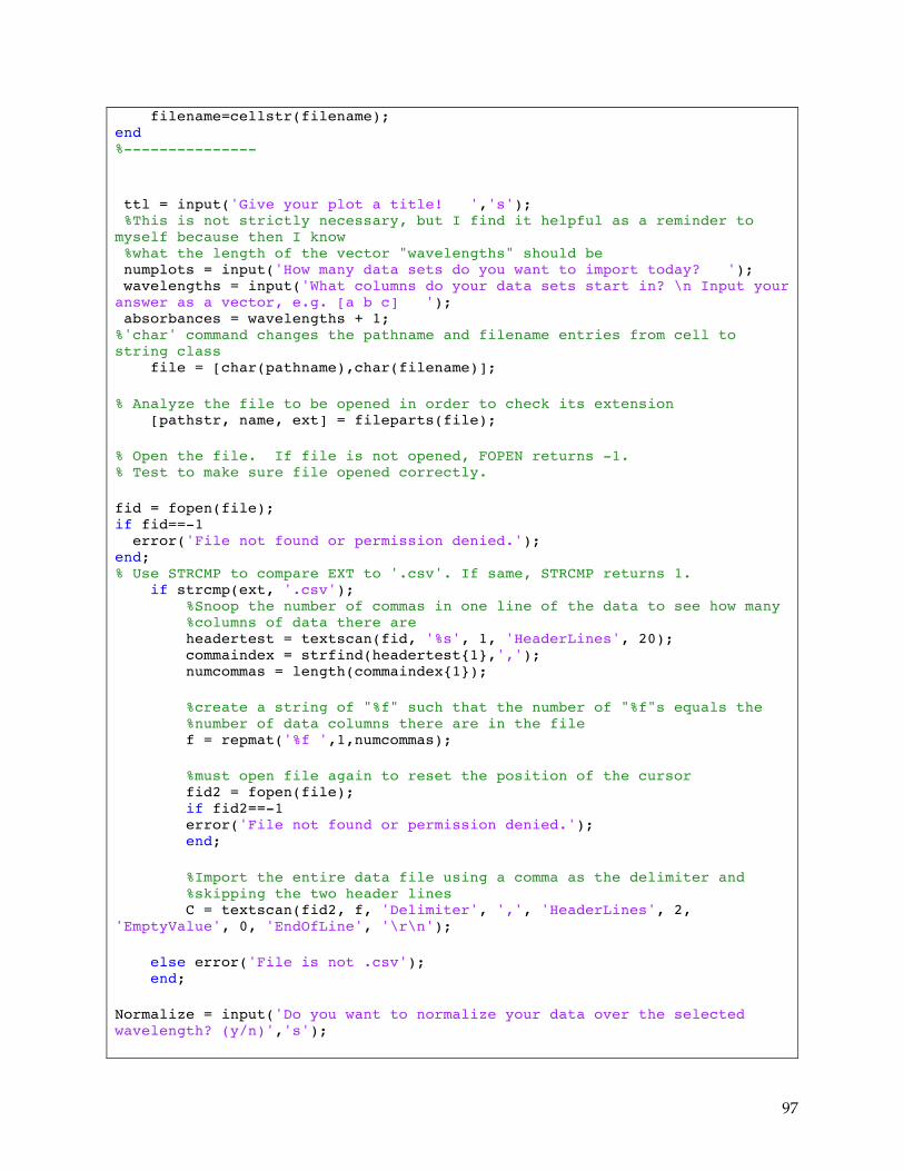
97
filename=cellstr(filename); end %--------------- ttl = input('Give your plot a title! ','s'); %This is not strictly necessary, but I find it helpful as a reminder to myself because then I know %what the length of the vector "wavelengths" should be numplots = input('How many data sets do you want to import today? '); wavelengths = input('What columns do your data sets start in? \n Input your answer as a vector, e.g. [a b c] '); absorbances = wavelengths + 1; %'char' command changes the pathname and filename entries from cell to string class file = [char(pathname),char(filename)]; % Analyze the file to be opened in order to check its extension [pathstr, name, ext] = fileparts(file); % Open the file. If file is not opened, FOPEN returns -1. % Test to make sure file opened correctly. fid = fopen(file); if fid==-1 error('File not found or permission denied.'); end; % Use STRCMP to compare EXT to '.csv'. If same, STRCMP returns 1. if strcmp(ext, '.csv'); %Snoop the number of commas in one line of the data to see how many %columns of data there are headertest = textscan(fid, '%s', 1, 'HeaderLines', 20); commaindex = strfind(headertest{1},','); numcommas = length(commaindex{1}); %create a string of "%f" such that the number of "%f"s equals the %number of data columns there are in the file f = repmat('%f ',1,numcommas); %must open file again to reset the position of the cursor fid2 = fopen(file); if fid2==-1 error('File not found or permission denied.'); end; %Import the entire data file using a comma as the delimiter and %skipping the two header lines C = textscan(fid2, f, 'Delimiter', ',', 'HeaderLines', 2, 'EmptyValue', 0, 'EndOfLine', '\r\n'); else error('File is not .csv'); end; Normalize = input('Do you want to normalize your data over the selected wavelength? (y/n)','s');
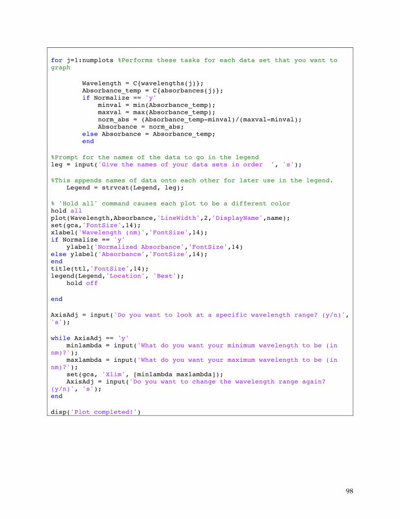
98
for j=1:numplots %Performs these tasks for each data set that you want to graph Wavelength = C{wavelengths(j)}; Absorbance_temp = C{absorbances(j)}; if Normalize == 'y' minval = min(Absorbance_temp); maxval = max(Absorbance_temp); norm_abs = (Absorbance_temp-minval)/(maxval-minval); Absorbance = norm_abs; else Absorbance = Absorbance_temp; end %Prompt for the names of the data to go in the legend leg = input('Give the names of your data sets in order ', 's'); %This appends names of data onto each other for later use in the legend. Legend = strvcat(Legend, leg); % 'Hold all' command causes each plot to be a different color hold all plot(Wavelength,Absorbance,'LineWidth',2,'DisplayName',name); set(gca,'FontSize',14); xlabel('Wavelength (nm)','FontSize',14); if Normalize == 'y' ylabel('Normalized Absorbance','FontSize',14) else ylabel('Absorbance','FontSize',14); end title(ttl,'FontSize',14); legend(Legend,'Location', 'Best'); hold off end AxisAdj = input('Do you want to look at a specific wavelength range? (y/n)', 's'); while AxisAdj == 'y' minlambda = input('What do you want your minimum wavelength to be (in nm)?'); maxlambda = input('What do you want your maximum wavelength to be (in nm)?'); set(gca, 'Xlim', [minlambda maxlambda]); AxisAdj = input('Do you want to change the wavelength range again? (y/n)', 's'); end disp('Plot completed!')

99
A.3 Fluorimeter data importer
Given the .XLS fluorimeter file type described in A.1, the function ‘extractxls’ takes user-defined
variable names to create matrix variables in the workspace representing the wavelength and
intensity data recorded by the fluorimeter. For example, the MATLAB input
‘[x,y]=extractxls;’ will open a window for the user to select a fluorimeter data output
file and will then create a matrix ‘x’ with the data set’s wavelengths and a matrix ‘y’ with the
accompanying intensity data. This data will then be plotted and the created matrix variables can
be saved or called for use in further analyses.
extractxls
function[t,y]=extractxls() [filename,pathname,filterindex]=uigetfile('*.*','MultiSelect','off'); M = xlsread(filename); t=M(:,1); y=M(:,2); plot(t,y)
A.4 UV-Vis data importer
Given the file type described in A.2, the function ‘extractcsv’ takes user-defined variable names
and a user-defined data location within the Excel file to create matrix variables in the workspace
representing the wavelength and absorbance intensity recorded by the spectrometer. For
example, the MATLAB input ‘[x,y]=extractcsv(1);’ will open a window for the user to
select a UV-Vis data output file and will then create a matrix ‘x’ with the wavelength data
from Column A of that file and a matrix ‘y’ with the accompanying absorbance data from
Column B of that file. The created matrix variables can be saved or called for use in further
analyses.
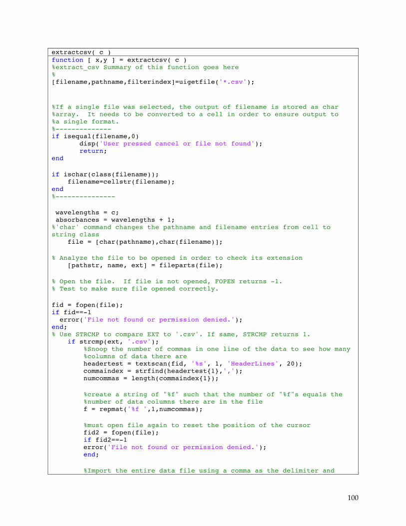
100
extractcsv( c ) function [ x,y ] = extractcsv( c ) %extract_csv Summary of this function goes here % [filename,pathname,filterindex]=uigetfile('*.csv'); %If a single file was selected, the output of filename is stored as char %array. It needs to be converted to a cell in order to ensure output to %a single format. %-------------- if isequal(filename,0) disp('User pressed cancel or file not found'); return; end if ischar(class(filename)); filename=cellstr(filename); end %--------------- wavelengths = c; absorbances = wavelengths + 1; %'char' command changes the pathname and filename entries from cell to string class file = [char(pathname),char(filename)]; % Analyze the file to be opened in order to check its extension [pathstr, name, ext] = fileparts(file); % Open the file. If file is not opened, FOPEN returns -1. % Test to make sure file opened correctly. fid = fopen(file); if fid==-1 error('File not found or permission denied.'); end; % Use STRCMP to compare EXT to '.csv'. If same, STRCMP returns 1. if strcmp(ext, '.csv'); %Snoop the number of commas in one line of the data to see how many %columns of data there are headertest = textscan(fid, '%s', 1, 'HeaderLines', 20); commaindex = strfind(headertest{1},','); numcommas = length(commaindex{1}); %create a string of "%f" such that the number of "%f"s equals the %number of data columns there are in the file f = repmat('%f ',1,numcommas); %must open file again to reset the position of the cursor fid2 = fopen(file); if fid2==-1 error('File not found or permission denied.'); end; %Import the entire data file using a comma as the delimiter and
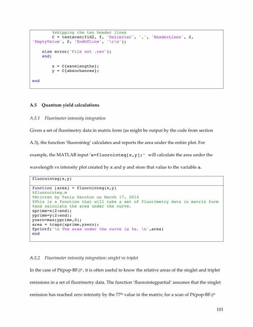
101
%skipping the two header lines C = textscan(fid2, f, 'Delimiter', ',', 'HeaderLines', 2, 'EmptyValue', 0, 'EndOfLine', '\r\n'); else error('File not .csv'); end; x = C{wavelengths}; y = C{absorbances}; end
A.5 Quantum yield calculations
Fluorimeter intensity integration
Given a set of fluorimetry data in matrix form (as might be output by the code from section
A.3), the function ‘fluorointeg’ calculates and reports the area under the entire plot. For
example, the MATLAB input ‘a=fluorointeg[x,y];’ will calculate the area under the
wavelength vs intensity plot created by x and y and store that value to the variable a.
fluorointeg(x,y)
function [area] = fluorointeg(x,y) %fluorointeg.m %Written by Tania Darnton on March 17, 2014 %This is a function that will take a set of fluorimetry data in matrix form %and calculate the area under the curve. xprime=x(2:end); yprime=y(2:end); yzero=max(yprime,0); area = trapz(xprime,yzero); fprintf('\n The area under the curve is %s. \n',area) end
Fluorimeter intensity integration: singlet vs triplet
In the case of Pt(pop-BF2)4-, it is often useful to know the relative areas of the singlet and triplet
emissions in a set of fluorimetry data. The function ‘fluorointegpartial’ assumes that the singlet
emission has reached zero intensity by the 77th value in the matrix; for a scan of Pt(pop-BF2)4-
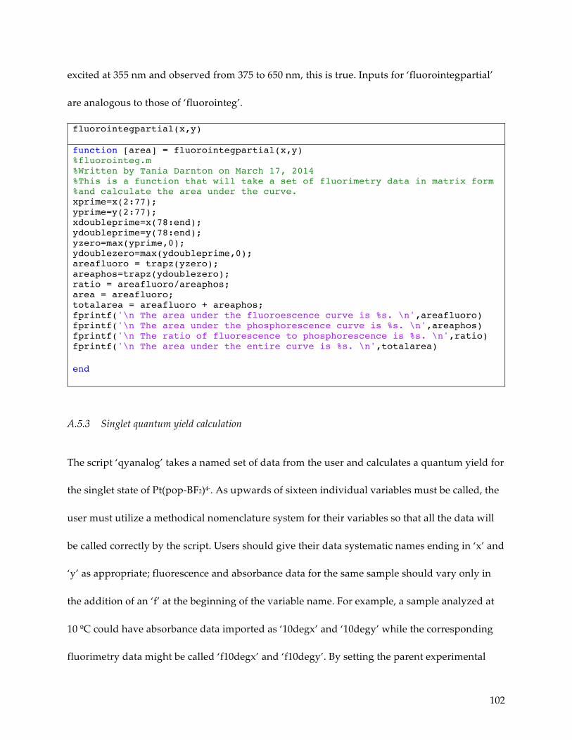
102
excited at 355 nm and observed from 375 to 650 nm, this is true. Inputs for ‘fluorointegpartial’
are analogous to those of ‘fluorointeg’.
fluorointegpartial(x,y)
function [area] = fluorointegpartial(x,y) %fluorointeg.m %Written by Tania Darnton on March 17, 2014 %This is a function that will take a set of fluorimetry data in matrix form %and calculate the area under the curve. xprime=x(2:77); yprime=y(2:77); xdoubleprime=x(78:end); ydoubleprime=y(78:end); yzero=max(yprime,0); ydoublezero=max(ydoubleprime,0); areafluoro = trapz(yzero); areaphos=trapz(ydoublezero); ratio = areafluoro/areaphos; area = areafluoro; totalarea = areafluoro + areaphos; fprintf('\n The area under the fluoroescence curve is %s. \n',areafluoro) fprintf('\n The area under the phosphorescence curve is %s. \n',areaphos) fprintf('\n The ratio of fluorescence to phosphorescence is %s. \n',ratio) fprintf('\n The area under the entire curve is %s. \n',totalarea) end
Singlet quantum yield calculation
The script ‘qyanalog’ takes a named set of data from the user and calculates a quantum yield for
the singlet state of Pt(pop-BF2)4-. As upwards of sixteen individual variables must be called, the
user must utilize a methodical nomenclature system for their variables so that all the data will
be called correctly by the script. Users should give their data systematic names ending in ‘x’ and
‘y’ as appropriate; fluorescence and absorbance data for the same sample should vary only in
the addition of an ‘f’ at the beginning of the variable name. For example, a sample analyzed at
10 ºC could have absorbance data imported as ‘10degx’ and ‘10degy’ while the corresponding
fluorimetry data might be called ‘f10degx’ and ‘f10degy’. By setting the parent experimental
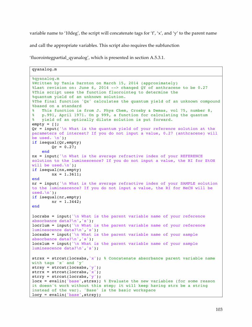
103
variable name to ‘10deg’, the script will concatenate tags for ‘f’, ‘x’, and ‘y’ to the parent name
and call the appropriate variables. This script also requires the subfunction
‘fluorointegpartial_qyanalog’, which is presented in section A.5.3.1.
qyanalog.m
%qyanalog.m %Written by Tania Darnton on March 15, 2014 (approximately) %Last revision on: June 6, 2014 --> changed QY of anthracene to be 0.27 %This script uses the function fluorointeg to determine the %quantum yield of an unknown solution. %The final function 'Qx' calculates the quantum yield of an unknown compound %based on a standard % This function is from J. Phys Chem, Crosby & Demas, vol 75, number 8, % p.991, April 1971. On p 999, a function for calculating the quantum % yield of an optically dilute solution is put forward. empty = []; Qr = input('\n What is the quantum yield of your reference solution at the parameters of interest? If you do not input a value, 0.27 (anthracene) will be used. \n'); if isequal(Qr,empty) Qr = 0.27; end nx = input('\n What is the average refractive index of your REFERENCE solution to the luminescence? If you do not input a value, the RI for EtOH will be used.\n'); if isequal(nx,empty) nx = 1.3611; end nr = input('\n What is the average refractive index of your SAMPLE solution to the luminescence? If you do not input a value, the RI for MeCN will be used.\n'); if isequal(nr,empty) nr = 1.3442; end locrabs = input('\n What is the parent variable name of your reference absorbance data?\n','s'); locrlum = input('\n What is the parent variable name of your reference luminescence data?\n','s'); locsabs = input('\n What is the parent variable name of your sample absorbance data?\n','s'); locslum = input('\n What is the parent variable name of your sample luminescence data?\n','s'); strsx = strcat(locsabs,'x'); % Concatenate absorbance parent variable name with tags 'x' and 'y' strsy = strcat(locsabs,'y'); strrx = strcat(locrabs,'x'); strry = strcat(locrabs,'y'); locx = evalin('base',strsx); % Evaluate the new variables (for some reason it doesn't work without this step; it will keep having strx be a string instead of the var). 'Base' is the basic workspace locy = evalin('base',strsy);
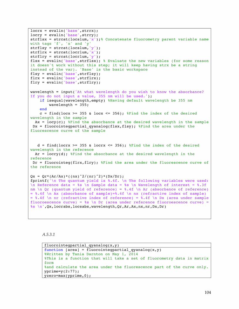
104
locrx = evalin('base',strrx); locry = evalin('base',strry); strflsx = strcat(locslum,'x');% Concatenate fluorometry parent variable name with tags 'f', 'x' and 'y' strflsy = strcat(locslum,'y'); strflrx = strcat(locrlum,'x'); strflry = strcat(locrlum,'y'); flsx = evalin('base',strflsx); % Evaluate the new variables (for some reason it doesn't work without this step; it will keep having strx be a string instead of the var). 'Base' is the basic workspace flsy = evalin('base',strflsy); flrx = evalin('base',strflrx); flry = evalin('base',strflry); wavelength = input('At what wavelength do you wish to know the absorbance? If you do not input a value, 355 nm will be used.'); if isequal(wavelength,empty) %Having default wavelength be 355 nm wavelength = 355; end c = find(locx >= 355 & locx <= 356); %Find the index of the desired wavelength in the sample Ax = locy(c); %Find the absorbance at the desired wavelength in the sample Dx = fluorointegpartial_qyanalog(flsx,flsy); %Find the area under the fluorescence curve of the sample d = find(locrx >= 355 & locrx <= 356); %Find the index of the desired wavelength in the reference Ar = locry(d); %Find the absorbance at the desired wavelength in the reference Dr = fluorointeg(flrx,flry); %Find the area under the fluorescence curve of the reference Qx = Qr*(Ar/Ax)*((nx)^2/(nr)^2)*(Dx/Dr); fprintf('\n The quantum yield is %.4f. \n The following variables were used: \n Reference data = %s \n Sample data = %s \n Wavelength of interest = %.3f nm \n Qr (quantum yield of reference) = %.4f \n Ar (absorbance of reference) = %.4f \n Ax (absorbance of sample)=%.4f \n nx (refractive index of sample) = %.4f \n nr (refractive index of reference) = %.4f \n Dx (area under sample fluoroescence curve) = %s \n Dr (area under reference fluoroescence curve) = %s \n',Qx,locrabs,locsabs,wavelength,Qr,Ar,Ax,nx,nr,Dx,Dr)
A.5.3.1
fluorointegpartial_qyanalog(x,y) function [area] = fluorointegpartial_qyanalog(x,y) %Written by Tania Darnton on May 1, 2014 %This is a function that will take a set of fluorometry data in matrix form %and calculate the area under the fluorescence part of the curve only. yprime=y(2:77); yzero=max(yprime,0);

105
area = trapz(yzero); end