structured prediction of generalized matching graphs · new york, ny 10027, usa ... dar and kearns,...
TRANSCRIPT
Journal of Machine Learning Research 1 (2008) 1-26 Submitted 3/08; Published ??/08
Structured Prediction of Generalized Matching Graphs
Stuart J. Andrews [email protected]
Tony Jebara [email protected]
Department of Computer ScienceColumbia UniversityNew York, NY 10027, USA
Editor: Leslie Pack Kaelbling
AbstractA structured prediction approach is proposed for completing missing edges in a graph using par-
tially observed connectivity between n nodes. Unlike previous approaches, edge predictions dependon the node attributes (features) as well as graph topology. To overcome unrealistic i.i.d. edge pre-diction assumptions, the structured prediction framework is extended to an output space of directedsubgraphs that satisfy in-degree and out-degree constraints. An efficient cutting plane algorithmis provided which interleaves the estimation of an edge score function with exact inference of themaximum weight degree-constrained subgraph. Experiments with social networks, protein-proteininteraction graphs and citation networks are shown.Keywords: Graph Inference, Structured Prediction, Generalized Matching, Transduction, Cutting-Planes
1. Introduction
Graphs are abstract models used to represent pairwise relationships between a set of objects. Inter-esting examples can be found in natural language processing, social networks, as well as in structuraland systems biology. Nodes represent individual objects, while edges encode relationships betweenpairs of objects. In practice, the nodes and edges have attributes associated with them too. Forexample, a collection of documents forms a graph called a citation network wherein nodes repre-sent papers, and directed connections between nodes represent citations between papers. What iscommon across many applied domains is the understanding that the likelihood or plausibility of agraph depends on both the attributes of the nodes and edges as well as the structure or topology ofthe graph connectivity implied by the edges.
The goal of this article is graph inference and reconstruction. In other words, filling in missingrelationships in a graph, assuming that some are known and others are hidden. Given a partially ob-served connectivity between n objects, the goal is to complete the connectivity to produce a realisticgraph. This discovery of new or missing interactions is important to many applied disciplines. Forinstance, there are practical implications for the recovery of new interactions in biological networksas well as the prediction of human preferences or relationships from partially completed social net-works. Examples of graph reconstruction efforts in biology are numerous ranging from metabolicnetworks (Herrgaard et al., 2004, Vitkup et al., 2006, Chechik et al., 2007), molecular networks(Baldi et al., 1999, Punta and Rost, 2005, Gassend et al., 2007), regulatory networks (Middendorfet al., 2004), and cell signaling networks (Sachs et al., 2005). Edge prediction is also relevant to
c©2008 Stuart J. Andrews and Tony Jebara.

ANDREWS AND JEBARA
a wider range of structured prediction problems that can also be cast as graph problems includingsentence parsing and image processing.
In previous approaches, edge predictions or graph reconstruction typically depends either onintrinsic properties of the graph (topology) or on extrinsic attribute values (features), but rarely onboth simultaneously. For example, metric learning can be viewed as a graph reconstruction methodand has recently had considerable progress in the machine learning community (Xing et al., 2003,Kondor and Jebara, 2006, Shalev-Shwartz et al., 2004, Globerson and Roweis, 2006). Typically, anaffinity or metric is learned between pairs of examples such that pairs of objects in an equivalenceclass have high similarity while those in different classes produce low similarity. To perform graphinference, pairwise similarity above a threshold indicates the presence of an edge between a pair ofobjects. However, using a learned affinity metric in a strictly pairwise manner makes all connectivitydecisions independently in the graph. Clearly, in realistic scenarios, the presence or absence of oneedge in a graph influences and depends on the presence or absence of other edges in the graph.Thus, an affinity metric alone may produce graphs whose structure is unlike that of realistic graphs.
Alternatively, in parallel efforts such as (Liben-Nowell and Kleinberg, 2003), topology is used topredict new edges in time-evolving citation networks. Exploiting topology is plausible since manyreal-world graphs exhibit a high degree of structural regularity. For instance, social network graphshave consistently small diameters and/or characteristic degree distributions. Complex biologicalsystems graphs are composed of frequently occurring motifs (Kashtan et al., 2004). Indeed, manygenerative models have been proposed that can replicate similar networks and their evolution (Even-Dar and Kearns, 2006).
Therefore, it is worthwhile to augment both schools of thought by combining independentnode/edge attribute learning methods with structural algorithms to preserve the regularities seen inreal-world graphs. In this paper, we present an algorithm for the prediction of naturally structuredgraphs using both topology and attribute data, which is based on a novel coupling of the structured-outputs framework (Altun et al., 2003, Taskar et al., 2003, Altun et al., 2004, Tsochantaridis et al.,2004, Altun et al., 2005, Taskar et al., 2006) and the class of degree-constrained subgraphs. Ourmodel learns to predict connectivity of ordered pairs of objects while enforcing in-degree and out-degree constraints. We show that by analyzing edge attributes while concurrently enforcing topo-logical structure constraints, our model yields a better predictor for graph connectivity. We believethat our model is the first to combine topology and attribute-value learning to significant advantagefor graph completion.
Our approach also presents a novel transductive variant of the structured-outputs frameworkto address graph completion. Transduction has previously been studied (Altun et al., 2005, Zienet al., 2007) to help design better structured predictors; however, these methods use labeled andunlabeled structured objects that are independent. The assumption is, for example, that the parsetree of one sentence does not depend on another and can therefore be predicted independently. Incontrast, our model considers transduction within a single structured object, a graph over n objects.Edges in the graph are either labeled or unlabeled however, transduction leverages the assumptionthat all labels are constrained by a single structure and all edge predictions are inter-dependent.This transductive inference of degree constrained graphs or generalized matchings is ultimatelyinterleaved in a cutting-plane structured prediction framework to complete real graphs.
This paper is organized as follows. Section 2 introduces graph completion in a formal setting.Next, in Sections 3 and 4, we discuss inference and learning within a maximum margin structuredoutputs framework. Section 5 discusses a number of implementation details of interest to practi-
2

STRUCTURED PREDICTION OF GENERALIZED MATCHINGS
tioners. In Section 6 we demonstrate the approach using synthetic and real-world graphs. Finally,to wrap up, Section 7 discusses related work, before some concluding remarks are presented inSection 8.
2. Graph Completion
In general, we are given a fixed set of nodes V = {1, . . . , n} which may be connected by a maximalset E = {(j, k) |1 ≤ j, k ≤ n} of n2 directed edges, if we allow self-loops. Binary edge labelsyj,k ∈ {0, 1} indicate the presence or absence of edge (j, k), while edge attributes are representedby a feature vector xj,k ∈ Rd. In the sequel, we occasionally refer to edges as being positive ornegative even though we are using 0-1 binary labels. We denote by X the set of all edge featurevectors and by Y the set of all labels.
Graph inference concerns the prediction of missing or unobserved edge labels from Y, assumingwe have observed only some of the entries together with the information encoded in the featuresX. Let O be the set of observed edges, U be the set of unobserved edges, where typically thepartition of edges satisfies O ∪ U = E . Because some of the labels are observed, and the goal is topredict the remaining labels, this process is also called completion. For example, suppose we haveV = {1, 2, 3} and we observe YO = {y1,1, y1,2, y2,1, y2,2}, then we would like to complete thenetwork by predicting values for YU = {y1,3, y2,3, y3,1, y3,2, y3,3}.
In the literature, several variants of the graph completion problem that depend on the choice ofO and U have been proposed. We describe four tasks, which are based on bipartite partitions, andone that is non-bipartite. Each bipartite task starts with a train-test partition of the nodes, whichinduces a block decomposition of the n×n adjacency matrix representation of the graph edges (seeFigure 1). We refer to the four blocks in the decomposition as: train-train, train-test, test-test andtest-train.
In (Yamanishi et al., 2004), the set O is comprised of train-train edges, while the set U iscomprised of the remaining blocks: train-test, test-test and test-train. In (Airoldi et al., 2007), thesetO is comprised of train-train edges, while the set U is comprised of the test-test edges. Finally, in(Bleakley et al., 2007), the setO is comprised of train-train edges, while the set U is comprised of allthe remaining blocks except the test-test edges. These graph completion tasks, which serve distinctbut related purposes, are depicted in Figure 2, columns (a-c). Two additional completion tasks aredisplayed in columns (d) and (e), the last being non-bipartite in the sense described above. As faras prediction is concerned, the number and variety of completion tasks present unique challenges tobe solved. Figure 2 provides an alternative depiction of the graph completion task from column (a)for a graph with a clear geometric structure. In this case, one half of the nodes (1-12) are observedyielding a partition of positive and negative training edges (middle row) and positive and negativetesting edges (bottom row).
2.1 A Probabilistic Model
We first start with a probabilistic treatment of the problem. The most naive assumption is that thedistribution p (Y|X) is parameterized by some unknown w and is independent across all Y entriesand factorizes as follows
pw (Y|X) =1
Zw (X)
∏j,k
φw (yj,k|xj,k) , (1)
3

ANDREWS AND JEBARA
trai
n
5 10 15 20
5
10
15
20
5 10 15 20
5
10
15
20
5 10 15 20
5
10
15
20
5 10 15 20
5
10
15
20
5 10 15 20
5
10
15
20Neg
Null
Pos
test
5 10 15 20
5
10
15
20
(a)5 10 15 20
5
10
15
20
(b)5 10 15 20
5
10
15
20
(c)5 10 15 20
5
10
15
20
(d)
5 10 15 20
5
10
15
20Neg
Null
Pos
(e)
Figure 1: Supervised graph completion predicts missing edges in a graph using partially observedconnectivity. Each column depicts an instance of the problem, where the top row showsthe edges that are observed and the bottom row shows the edges that are missing. Blackand white matrix entries indicate positive (on) and negative (off) edges, while grey entriesare excluded from consideration. The semantics are (a) extending or growing a network,(b) predicting a similar but independent network, (c) linking new nodes to an existingnetwork, and (d) linking two networks. The last column shows (e) an example of a non-bipartite partition (see text).
and Zw (X) is the normalization constant. For instance, we may assume that the presence or absenceof a edge depends on the feature vector xj,k associated with the nodes it connects, and a parameterw by way of a log-linear potential function
φw (yj,k|xj,k) = exp((
wTxj,k
)yj,k
). (2)
However, since some connectivity structures are more likely than others, the independence assump-tion is too simple. More realistically, there are dependencies between the labels. For instance,consider a set of cliques c ∈ C over the edge labels in Y. This gives the probability distribution
pw (Y|X) =1Z
∏c∈C
φc (yc)∏j,k
φw (yj,k|xj,k) , (3)
where each φc is a multivariate clique potential function over a set of edges. By choosing differentforms for the φc, we can tailor our beliefs about which network topologies are more plausible thanothers.
Given a setting of w, the problem of finding the most likely completion of a partially observednetwork amounts to solving
argmaxYU
pw (YU |YO,X) = argmaxYU
pw (YU ,YO|X) . (4)
4

STRUCTURED PREDICTION OF GENERALIZED MATCHINGS
com
plet
e
1
2
3
4
5
6
7
8
9
10
11 12
13
14
15
16
17
18 19
20
21
22
23
24
1
2
3
4
5
6
7
8
9
10
11 12
13
14
15
16
17
18 19
20
21
22
23
24tr
ain
1
2
3
4
5
6
7
8
9
10
11 12
13
14
15
16
17
18 19
20
21
22
23
24
1
2
3
4
5
6
7
8
9
10
11 12
13
14
15
16
17
18 19
20
21
22
23
24
test
1
13
14
15
16
17
18 19
20
21
22
23
24
2
3
4
5
6
7
8
9
10
11 12
1
13
14
15
16
17
18 19
20
21
22
23
24
2
3
4
5
6
7
8
9
10
11 12
positive negative
Figure 2: Graph inference on a structured graph. (Top-left) 24 equally spaced nodes on a circle areconnected by positive edges running in a counter clockwise direction. As depicted in (top-right) using dashed lines, there are many more negative edges exhibiting a complementarystructure. In a typical graph inference setting, a subset of the nodes and their connectivityare observed. In this case, one half of the graph nodes numbered 1-12 are observedresulting in (middle-left) positive and (middle-right) negative edges available for training.The goal is to correctly classify the remaining edges into positive and negative categories,as shown in (bottom-left) and (bottom-right) respectively.
5

ANDREWS AND JEBARA
Solving Equation (4) is typically called inference. A more challenging problem is that of learningthe parameters w from data. For learning, we use the observed edge features X and the partiallyobserved connectivity in YO as training data. The first objective in learning w is to ensure that theconnectivity predicted by the model matches that of YO. The second objective is to ensure thatthe model is able to generalize by predicting the correct labels for unobserved edges. A principledapproach to achieve this objective is maximum likelihood. The maximum likelihood estimate forthe parameter w is given by the following optimization problem which integrates over the unknownlabels
argmaxw
∑YU
pw (YU ,YO|X) . (5)
However, the quantity being maximized involves summing 2|YU | terms where |YU | is the cardinalityor the number of unknown labels and moreover the normalization constant Zw involves summing2|Y| terms where |Y| is n2. Even though many of the terms in the summations are zero, the nor-malization over these binary variables is computationally too difficult. An alternative approach toachieve the same goals is based on empirical risk minimization.
3. Generalized Matchings
In many applications of graph completions, the degree δi of each node is known or an accurate upperbound can be established. For example, when a structural biologist searches for the 3D structure ofa macromolecule, constraints are placed on the number and types of bonds that each molecular unitcan make. In the study of protein interactions (Kim et al., 2006), 3D shape analysis has been usedto bound the number of mutually accessible binding sites of a protein. In many social networks, thenumber of connections a user has made is advertised on their profile, even though the set of users towhom they connect is kept confidential (e.g. LinkedIn1).
Since in practice the degrees of nodes in a graph are often readily available, and because thisinformation is not currently used by existing methods for graph completion, we decided to studyif and how this topological information could be used to improve prediction. Thus, throughout theremainder of the paper, we assume that degree information is available for the graphs that are to becompleted. To this end, we consider a class of structured graphs called generalized matchings. LetG = (V, E) be a graph consisting of all candidate edges, for example, the complete graph over nnodes.
Definition 1 A generalized matching in a graph G = (V, E) is a subgraph defined by edge labelsY that satisfy in-degree and out-degree constraints. The set of generalized matching is definedprecisely as follows
B ,
{Y ∈ {0, 1}n
2
| yj,k = 0 if (j, k) /∈ E ,∑j
yj,k ≤ δink ,
∑k
yj,k ≤ δoutj , j, k = 1, . . . , n
}.
(6)
for given constants δink , δout
j ∈ {0, . . . , n}.
1. www.linkedin.com
6

STRUCTURED PREDICTION OF GENERALIZED MATCHINGS
We can use generalized matchings to further specify our probabilistic model of graphs. In this case,there will be a clique in the graphical model for each row and column of random variables fromthe adjacency matrix Y, and potential functions φin
k (Y) = H(δin
k −∑
j yjk
)and φout
j (Y) =
H(δout
j −∑
k yjk
)where H (·) is the Heaviside step function.2 Substituting these cliques into
Equation (3), the complete factorization of the model has the following form
pw (Y|X) ∝∏j
φinj (Y)
∏k
φoutk (Y)
∏j,k
φw (yj,k|xj,k) . (7)
Notice that the probability will be zero whenever the degree constraints are not met.For inference by Equation (4), the generalized matching inspired cliques effectively restrict our
search to Y = YU ∪YO ∈ B, since all other configurations have zero probability. Setting the edgescores sj,k = log (φw (yj,k|xj,k)) , predictions can then be made by solving
GM : argmaxYU
∑j,k
sj,kyj,k s.t. Y ∈ B , (8)
which is a 0-1 programming problem. The quantity∑
j,k sj,kyj,k =∑
j,k
(wTxj,k
)yj,k is called
the score of the generalized matching specified by Y.The GM problem has been studied extensively in operations research, and is closely related to
methods recently applied in machine learning. If the degrees are δink = δout
j = 1, in addition tothe graph being bipartite and symmetric, then the set of degree-constrained subgraphs are exactlythe 1-matchings of G, which are used to learn structural alignments in (Chatalbashev et al., 2005,Taskar et al., 2005). In the 1-matching case, the iterative Hungarian or Kuhn-Munkres algorithmseach provide efficient solutions with worst case O
(n3
)time complexity. Moreover, it has been
shown that the optimal 0-1 solution is found by the linear programming relaxation of GM, which,given the quality of industrial LP solvers, is likely to be faster still.
While in general, the GM problem with arbitrary degrees δink , δout
j is significantly more com-plex, remarkably, it has be reduced to a balanced network flow problem, resulting in O
(n3
)com-
plexity. A primal-dual solver for this class of problems is available in the Goblin package (Fremuth-Paeger and Jungnickel, 1998). This solver accepts both upper and lower bounds on the degrees,has options for directed or undirected graphs, and also operates on large sparse graphs. Using thesparse solver allows us to predict missing edges without incurring theO
(n3
)cost of solving for the
complete graph connectivity.
4. Learning
In typical methods for graph completion, the edge scores sj,k depend in some way on the nodesimilarity and the edge attributes. Previous researchers have proposed and debated the merits ofvarious node similarity or correlation scores. Instead of relying on our ability to design such scoringfunctions by hand, we propose to select the scoring function from a large family of candidates, ina data-driven manner. In particular, we assume a scoring function sj,k =
(wTxj,k
)that depends
linearly on the features via hyperplane parameter w and adopt a discriminative structured-outputs
2. The Heaviside step function is defined by H(t) =
(1 t ≥ 0
0 t < 0.
7
ANDREWS AND JEBARA
framework (Taskar et al., 2003, Tsochantaridis et al., 2004) in order to learn the weight vector wfrom data. Structured output models developed within the max-margin framework have been suc-cessfully applied to predicting part-of-speech tags, word-alignments, parse trees and image segmen-tations (Tsochantaridis et al., 2004, Taskar et al., 2004a, 2005). By focusing effort on the margin,these formulations provide a tractable alternative to conditional likelihood modeling which wouldotherwise require the computation of a partition function (Lafferty et al., 2001).
We begin by learning a weight vector that can predict the edges in O. Consider a fixed but un-known distribution P (X,Y) over generalized matchings. We would like to select a score functionso that the true connectivity Y achieves a larger score than any alternative set of labels Z ∈ B withZO 6= YO ∑
j,k∈O
(wTxj,k
)yj,k ≥
∑j,k∈O
(wTxj,k
)zj,k , ∀Z ∈ B, ZO 6= YO (9)
for any sample (X,Y) drawn from P (X,Y). If the weight vector w is chosen to satisfy Equa-tion (9), then the inference procedure will predict Y = argmaxZ∈B
∑j,k∈O wTxj,kzj,k equal to
the correct graph Y, otherwise an error is incurred.The structured-outputs framework attempts to minimize the probability of error by maximizing
a margin quantity γw = γw (X,Y) measured on the training data. Generalizing the multi-class caseof (Crammer and Singer, 2001), the margin quantity is defined as the minimum difference betweenthe score of the true connectivity and an alternative connectivity
γw (X,Y) ≤∑
j,k∈OwTxj,kyj,k −
∑j,k∈O
wTxj,kzj,k , ∀Z ∈ B, ZO 6= YO . (10)
The problem of maximizing the margin γw over bounded weight vectors w is equivalent to thefollowing optimization problem
minw
12‖w‖2
s.t.∑
j,k∈OwTxj,kyj,k ≥
∑j,k∈O
wTxj,kzj,k + ∆0/1 (Y,Z) , ∀Z ∈ B ,(11)
where we have introduced the 0/1 loss term ∆0/1 (Y,Z) and eliminated the restriction on ZO. As iscommon for structured-outputs learning, two further modifications are made to this maximum mar-gin formulation. First, the Hamming loss ∆H (Y,Z) is substituted for the 0/1 loss ∆0/1 (Y,Z) withthe goal of improving generalization (Taskar et al., 2006). The Hamming loss ∆H (Y,Z), countsthe number of edge prediction errors
∑j,k zj,k (1− yj,k) + yj,k (1− zj,k) and can be expressed as∑
j,k ∆j,kzj,k + ∆0 for given numbers ∆0, ∆j,k depending on yj,k. Finally, a slack variable ξ isintroduced to allow for potential violations of the margin constraint, with a scaled penalty in theobjective. The resulting learning problem is
CUTSVM :minw,ξ
12‖w‖2 + Cξ
s.t.∑
j,k∈OwTxj,kyj,k ≥
∑j,k∈O
(wTxj,k + ∆j,k
)zj,k + ∆0 − ξ , ∀Z ∈ B .
(12)
Notice that the slack variables are constrained to be positive ξ ≥ 0 because we include the possibilityof Z = Y in these constraints. More importantly, notice that the terms in the constraints involvesummations over the training points only.
8

STRUCTURED PREDICTION OF GENERALIZED MATCHINGS
While we have derived our formulation using the structured prediction framework, it is interest-ing to note that the final optimization problem bears striking resemblance to the recently proposed1-slack formulation of the support vector machine (Joachims, 2006), which is implemented in SVM-perf. Using the edge data (xj,k, yj,k) as independent examples, the 1-slack formulation considers2n2
possible linear constraints that are indexed by n2 binary variables cj,k 1 ≤ j, k ≤ n. In ourwork, constraints are also indexed in the same way through zj,k , yj,k − cj,k, but the total numberof possible constraints is less than 2n2
because the Z variables are constrained to be generalizedmatchings. We compare the performance of CUT-SVM against SVM-perf, not only because SVM-perf is the exact i.i.d. counterpart of CUT-SVM, but also because SVM-perf is capable of solvinglarge SVM problems such as those encountered in pairwise classification tasks dealing with n2
pairs.
4.1 The Cutting-Plane Algorithm
At first glance, solving CUTSVM is a formidable task due to the super-exponential number oflinear constraints that define the space of feasible solutions w. Using the technique of cutting-planes, however, we can find an approximate solution that is within a pre-specified tolerance of theoptimum, in a finite number of steps (Tsochantaridis et al., 2004, Joachims, 2006).
The key idea employed by cutting-plane algorithms is that we are not so much interested inrepresenting the complete feasible region, but instead finding a good approximation to it near theoptimal solution (Kelley, 1960). The algorithm works in rounds, generating a nested sequence ofapproximations F1 ⊇ . . . ⊇ Ft to the true feasible region, and returning the optimal solution(wt, ξt) for the current approximation. The regions Ft are defined by a growing subset of the origi-nal constraints, called the cut set C. Each round selects the most violated of the original constraintsindexed by Z ∈ B, and adds this constraint to the cut set C, thereby shrinking the feasible regionFt+1. The algorithm terminates when there are no remaining constraints that are violated by morethan the allowed tolerance ε ≥ 0.
Cut generation, the task of finding the most violated constraint, reduces to a GM subproblemusing the loss-augmented edge scores
(wTxj,k + ∆j,k
)Zt = argmax
Z∈B
∑j,k∈O
(wTxj,k + ∆j,k
)zj,k (13)
Notice again that the GM optimization is performed over the observed subset of edges alone.We write CUTSVM (C, C) to denote the solution of quadratic programming problem from Equa-tion (12) with slack penalty C but limited to the subset of constraints Z ∈ C. For typical prob-lems and with a large enough tolerance ε, the number of constraints in C is manageable andCUTSVM (C, C) can be solved efficiently. CUTSVM (C, C) may also be initialized with the solu-tion from the previous iteration. The complete algorithm is shown in the box.
4.2 Transductive Cut Generation
In a general graph completion task, we observe (X,YO) and the goal is to complete the connectivityY by predicting the missing elements YU . Since the features for all edges, training and testing,are available during training, we can use the principle of transductive inference to help guide theselection of the score function, and to improve our ability to complete Y.
9

ANDREWS AND JEBARA
Algorithm 1 The cutting-plane algorithm for learning to predict generalized matchings.1: Input: Graph data (X,YO), slack penalty C, and cut tolerance ε ≥ 0.2: (w1, ξt)← (0, 0), C ← ∅, t← 03: repeat4: Zt ← argmaxZ∈B
∑j,k∈O
(wTxj,k + ∆j,k
)zj,k
5: if∑
j,k∈O wTxj,kyj,k ≤∑
j,k∈O(wTxj,k + ∆j,k
)zj,k + ∆0 − ξ − ε then
6: C ← C ∪ {Zt}7: (wt+1, ξt+1)← CUTSVM (C, C)8: end if9: t← t + 1
10: until no change in C (i.e. all cuts satisfied within allowed tolerance ε)
In the maximum-margin framework, transductive inference is usually accomplished by max-imizing a margin quantity over both labeled and unlabeled examples (Gammerman et al., 1998,Joachims, 1999, Bennett and Demiriz, 1998, Collobert et al., 2005). Following this general ap-proach, we have modified the method by which cutting-planes are generated, allowing the test edgesto influence w in an indirect fashion. Ideally, we would include the test points when solving theGM with loss-augmented scores, simply by summing over U
Zt = argmaxZ∈B
∑j,k∈O∪U
(wTxj,k + ∆j,k
)zj,k . (14)
However, since the entries of YU are not known, the loss terms ∆j,k can not be computed for(j, k) ∈ U . Our proposed solution is to first predict values VU = YU using the current scores
Vt = argmaxV∈B,VO=YO
∑j,k∈O∪U
wTxj,kvj,k , (15)
and then to compute the loss terms ∆j,k using our predicted labels from VU . Substituting these∆j,k back into Equation (14), we obtain an alternative structure Zt that approximates the optimalloss augmented generalized matching. As far as the cutting-plane algorithm is concerned uponthe receipt of Zt, it has obtained another violated constraint corresponding to a valid generalizedmatching structure; only the observed component ZO is considered further.
5. Implementation Details
This section discusses a number of issues that arise when implementing the cutting-plane algorithmfor learning to predict generalized matchings.
5.0.1 SCORE COMPUTATION
A significant computational aspect of CUT-SVM is the calculation, each iteration, of the edge scoressj,k = wTxj,k ,∀j, k , which requires O
(n2d
)operations, where d the feature dimension. This
issue is compounded by that fact that d may be large, and so the complete set of features may not fitin memory. For the large graphs that we studied, we were able to store attributes of each node, andrecompute the edge features xj,k = f (xj ,xk) on the fly.
10
STRUCTURED PREDICTION OF GENERALIZED MATCHINGS
5.0.2 NEGATIVE SCORES
It is easy to show that exact inference will never select edges that have negative scores; omitting theedge would result in a higher scoring graph that also satisfies the upper degree constraints. There-fore, we could remove edges with negative scores in order to speed-up certain generalized matchingsolvers. However, such thresholding complicates CUT-SVM learning because the structures Zt willhave varying numbers of edges, which in turn introduces uneven biases through the linear terms∑
j,k xj,k (yj,k − zj,k) of the constraints.Ideally, we would like the matching solver to be invariant to positive or negative shifts of the
score values. One solution is to change the definition of generalized matchings to use equality con-straints instead of upper degree bounds, thus ensuring that all structures Zt have the same numberof edges even though some of their scores are negative. Two difficulties of this approach are first,that the matching solver may not support equality constraints, and second, the degree constraintsmay become impossible to satisfy if the degrees are estimated poorly. Moreover, in practice it ismuch more reasonable to derive an upper bound on the degree, rather than its exact value. Hence,the alternative solution that is adopted here is to constrain the scores to be positive, and use upperdegree bounds in the definition of the generalized matchings as in Equation (6). One method to en-sure positive scores is to use only positive features, and additionally, to constrain the weight vectorto be positive. An easier approach is to add a sufficiently large constant to the scores.
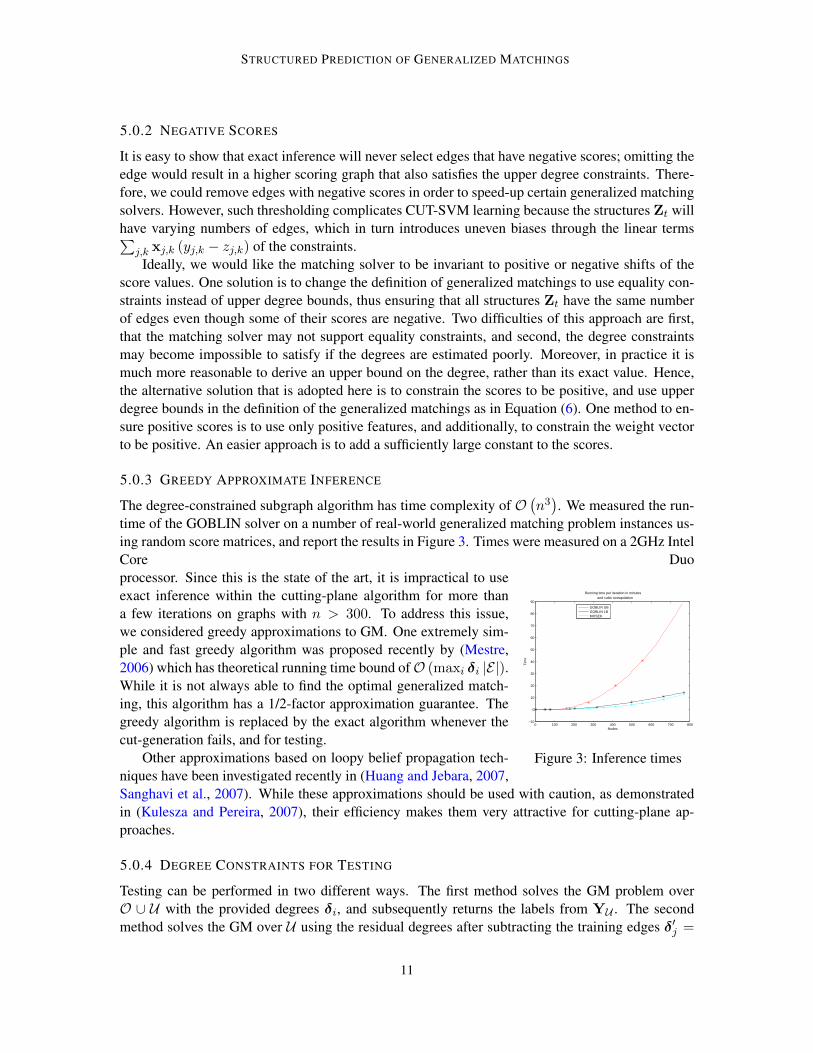
5.0.3 GREEDY APPROXIMATE INFERENCE
The degree-constrained subgraph algorithm has time complexity of O(n3
). We measured the run-
time of the GOBLIN solver on a number of real-world generalized matching problem instances us-ing random score matrices, and report the results in Figure 3. Times were measured on a 2GHz IntelCore Duo
0 100 200 300 400 500 600 700 800−10
0
10
20
30
40
50
60
70
80
90
Nodes
Tim
e
Running time per iteration in minutes and cubic extrapolation
GOBLIN UBGOBLIN LBMOSEK
Figure 3: Inference times
processor. Since this is the state of the art, it is impractical to useexact inference within the cutting-plane algorithm for more thana few iterations on graphs with n > 300. To address this issue,we considered greedy approximations to GM. One extremely sim-ple and fast greedy algorithm was proposed recently by (Mestre,2006) which has theoretical running time bound ofO (maxi δi |E|).While it is not always able to find the optimal generalized match-ing, this algorithm has a 1/2-factor approximation guarantee. Thegreedy algorithm is replaced by the exact algorithm whenever thecut-generation fails, and for testing.
Other approximations based on loopy belief propagation tech-niques have been investigated recently in (Huang and Jebara, 2007,Sanghavi et al., 2007). While these approximations should be used with caution, as demonstratedin (Kulesza and Pereira, 2007), their efficiency makes them very attractive for cutting-plane ap-proaches.
5.0.4 DEGREE CONSTRAINTS FOR TESTING
Testing can be performed in two different ways. The first method solves the GM problem overO ∪ U with the provided degrees δi, and subsequently returns the labels from YU . The secondmethod solves the GM over U using the residual degrees after subtracting the training edges δ′j =
11

ANDREWS AND JEBARA
δj −∑
k:(j,k)∈O yj,k, and subsequently returns the result YU . In practice was have found thatthe second method works better, probably because the resulting GM inference problem is moreconstrained.
6. Evaluation
One of the motivations of this work was to understand if, when, and where topological constraintscould be used to improve the prediction of missing edges in a partially observed graph. For thisreason, we tried to design a system that was capable of working with a wide range of network datasets. This required flexibility in handling directed and undirected edges as well as various sorts ofnode and edge attribute data.
6.1 Connectivity and Attribute Data
The graph data we considered included:
• Simple directed graphs embedded in R2 and R3 : these networks were synthetically generatedand included a circle, torus, star, etc.
• A directed cell-signaling network (Sachs et al., 2005): for this network, the expression levelsof 11 signaling molecules subjected to external stimuli were measured using a technologycalled flow cytometry. The network is defined by the causal influences of one molecule onanother. These have been determined through extensive and time consuming laboratory study.
• An undirected protein-interaction graph (Yamanishi et al., 2004), and an undirected enzyme-interaction graph (Yamanishi et al., 2005): these data sets are described by several n × nkernels, each encoding similarity of a biological attribute. The edges, which correspond tophysical or chemical interactions, are determined experimentally.
• A directed citation network from CoRA (McCallum et al., 2000): this database containsdocument attributes (e.g. abstract, authors’ names, date of publication, topic classification),in addition to a citation network (edges from one paper to another) for several thousand paperson machine learning.
• An undirected friendship graph from a social network: web pages and the accompanying“friendship” structure were manually downloaded in a neighbourhood a seed page.
We have tailored our model to handle both directed and undirected graphs independently, but we donot handle graphs that have both directed and undirected arcs. While self loops are handled, we didnot find an example where we needed to use them.
In all cases except the protein-interaction and enzyme-interaction examples, the attribute datawe collected were measurements associated with the nodes. For the embedded geometric graphs,we used the coordinates in space for the node features. The node attribute data for the cell-signalingnetwork are the expression levels of various molecules. For the citation and social network, theattribute data for the nodes consists of formatted text. In order to compress the bag-of-words rep-resentations from the citation network and the social network, we use latent Dirichlet allocation(LDA) (Griffiths and Steyvers, 2004). This resulted in a vector of 111 dimensions describing thedocuments in CoRA, and a 171 dimensional feature vector describing an individual user’s page.
12

STRUCTURED PREDICTION OF GENERALIZED MATCHINGS
k 1 2 3 4 5 6 7 8 9 10 11 12 14n 668 667 608 483 407 326 287 243 174 81 75 41 15
Table 1: The relationship between the size of the core and degree k.
The protein and enzyme data sets were instead described by several n× n kernels each. Whilethe kernel values themselves could be used as edge features, we adopted the empirical feature mapapproach in order to extract relevant features for the nodes. This was accomplished by decomposingthe kernel K = (kj,k) via eigendecomposition. The resulting features xj measure the similarity ofthe j-th node to a set of prototypes, like the empirical feature map (Tsuda, 1999).
In all cases except the signaling network, given a pair of nodes (j, k) we defined the featuresfor edge xj,k , vec
(xjxT
k
)using an outer product of the node features. The result is a high
dimensional representation for edges that includes all pairwise products between a feature fromj and a feature from k. In general xj,k 6= xk,j which provides an opportunity for the model todiscriminate edge directionality, if required by the task. For the signaling network, the edge featureswere constructed by hand for interpretability of the learned weight vector, and consistency withprevious work.
As mentioned earlier, we have assumed that accurate upper degree bounds can be estimatedin each application. Thus, for these preliminary experiments, we have used the true degree δi
calculated over the entire graph. In the subsequent sections, we describe experiments on geometricgraphs, protein-interaction graphs and cell-signaling graphs.
6.2 Experimental Protocol
We used the notion of the k-core of a graph to select subgraphs of manageable size for developmentpurposes and to observe behaviour of CUT-SVM closely. A core of a graph of degree k is theset of nodes and edges that remain after recursively pruning any node (and its edges) with degreeδ < k. The cores of a graph form a nested sequence, much like the various cores of an onion.The relationship between the degree k and the size of the core is shown in Table 1 for the enzyme-interaction graph from (Yamanishi et al., 2005).
We perform 5-fold cross-validation to evaluate and compare CUT-SVM and i.i.d. SVM usingone of the bipartite schemes from Figure 1. The bipartite partition of edges O ∪ U is determinedfrom the train-test partition of the nodes on each fold. Thus, we first divide the n nodes into 5subsets of roughly equal size. Then, on the k-th fold, the testing subset of nodes is determined bythe k-th subset, while the remaining nodes comprise the training subset.
The algorithms train on data (X,YO), and are evaluated based on their predictions for theunknown labels YU . We look at the area under the curve (AUC), accuracy and recall. For a faircomparison with CUT-SVM, the threshold of the i.i.d.-SVM classifier is chosen so that it predictsNtot =
∑i δi/2 edges, which is the same number of edges predicted by CUT-SVM. Since CUT-
SVM predicts 0-1 outputs, the threshold is alway fixed at 0.5. The cross validated performance fora given metric, is taken to be the average performance measured on the testing edges U across folds.
13

ANDREWS AND JEBARA
6.3 Results
6.3.1 COMPLETING THE CIRCLE EXPERIMENTS
The purpose of this example is to validate our algorithms. To generate the graph, we placed M = 24points on a circle centered on the origin with even spacing. These were connected using directededges in counter-clockwise order. The x-y coordinates of the points were used as node attributes.To make this example challenging, we used a random 2:3 partition of the nodes as can be seen in thetop row of the Figure. 4. If we use larger training sets, then each method described below obtainsnear-perfect performance.
We compared i.i.d.-SVM, CUT-SVM and CUT-SVM with transduction, using a slack penaltyC = 1. We used a fairly loose tolerance ε = 0.1. The bottom row of the figure shows the com-pletions predicted by these algorithms. The i.i.d.-SVM in (d) ignores the degree constraints andappears to have been confused by the 87 negative edges which far out-number the 3 positive ones.The CUT-SVM algorithm without transduction (d) does somewhat better primarily due to the useof the degree constraints. The training set is still too small to learn an accurate model, especiallygiven the loose tolerance ε. Finally, in (f) we see that the CUT-SVM with transduction has predictednearly all edges correctly. This is primarily due to the fact that the transductive model adapts itslearning to the presence of the test points.
6.3.2 ENZYME-ENZYME INTERACTIONS
We focus next on a completion task involving the enzyme-interaction network from (Yamanishiet al., 2005). We performed an eigendecomposition on the “gene expression”, “localization”, and“phylogenetic profile” kernels, keeping enough eigenbases to explain 50% of the variance of eachkernel, resulting in a 44 dimensional feature vector for each node. The outer product xjxT
k has 1936elements, however, since the network is undirected, symmetry constraints are used to reduce thisdimension to 990.
The core of size n = 81 was used for this experiment. We set ε = 0.05 and varied the slackparameter across the following values C = {1e2, 1e4, 1e6, 1e8, 1e10, 1e12, 1e14}. We initializedthe weight vector of the cutting-plane algorithm using the solution from i.i.d.-SVM.
In the following discussion, we describe in detail several aspects of the model, making referenceto the following figures.
• Figure 5 displays learning curves for just one of the many runs of CUT-SVM.
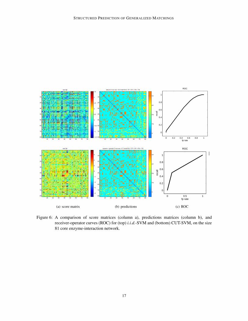
• Figure 6 compares the results of CUT-SVM with that of i.i.d.-SVM in terms of the learnedscores, the predictions and the ROC curves.
• Figure 7 details the behaviour of the algorithms across the range of C values.
To begin, observe how in Figure 5 (a) , the depth of the cutting-planes converges quickly in the firstiterations and yet remains positive with a long tail. This is a typical profile for a problem with manysimilar constraints, most of which are not active at the optimum. This behaviour also validates thefinite convergence theorems of (Tsochantaridis et al., 2004, Joachims, 2006). In (b) and (c), we seethe performance on the test edge, measured every 25 iterations. While these curves quickly leveloff, in the first few iterations there is significant improvement over the i.i.d.-SVM algorithm that isshown at iteration 0.
14

STRUCTURED PREDICTION OF GENERALIZED MATCHINGS
5 10 15 20
5
10
15
20
(a) training partition
1
2
3
4
5
6
78
9
10 11
12
1314
15
16
17
18
19
20
21
22
23
24
(b) positive training edges
1
2
3
4
5
6
78
9
10 11
12
1314
15
16
17
18
19
20
21
22
23
24
(c) negative training edges
1
2
3
4
5
6
78
9
10 11
12
1314
15
16
17
18
19
20
21
22
23
24
(d) i.i.d. SVM
1
2
3
4
5
6
78
9
10 11
12
1314
15
16
17
18
19
20
21
22
23
24
(e) CUT SVM
1
2
3
4
5
6
78
9
10 11
12
1314
15
16
17
18
19
20
21
22
23
24
(f) transductive CUT SVM
Figure 4: Completing the connectivity of a circle. The training subset, generated from a 2:3 splitof the nodes, is depicted in (a). The black entries indicate positive edges which are alsoshown in (b). The white entries indicate negative edge which are also shown in (c).The bottom row shows the predicted completions; the edges from the test set that werepredicted to be positive, in addition to the positive edges from the training set. False-positives are demarked by open arrows, which can be seen by magnifying the individualfigures. Results include (d) i.i.d. SVM, (e) CUT-SVM without using transduction, and(f) CUT-SVM using transduction.
15

ANDREWS AND JEBARA
0 50 100 150 200 250 300 3500
0.5
1
1.5
2
2.5cut depth
iter
(a) cut depth
0 100 200 300 4000.62
0.64
0.66
0.68
0.7
0.72AUC test
iter
(b) area under curve
0 100 200 300 4000.25
0.3
0.35
0.4
0.45
0.5
0.55
0.6top N recall test
iter
(c) recall
Figure 5: Learning curves for CUT-SVM on the size n = 81 core enzyme-interaction network.
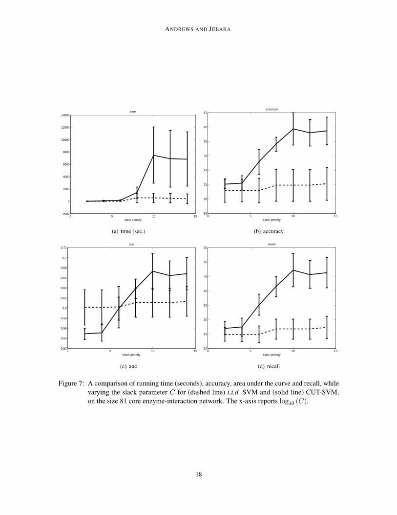
Clearly, the degree constraints are helping CUT-SVM. This effect is also evident in the scoreand prediction matrices in Figure 6 (a-b). The prediction matrix uses color entries to indicate howan edge is classified, with colors for true-positives (tp), true-negatives (tn), false-positives (fp), andfalse negatives (fn). The i.i.d.-SVM algorithm cannot help but learn a banded score matrix, and itwill make predictions that are similarly banded, which is evident from the Figure 6 (b). Figure 7provides a more complete view of the performance of both algorithms across a range of C values.The difference in the recall measure of the two algorithms is striking. For example, at the largest Cvalue the average recall of i.i.d.-SVM is 27.3 ± 3.9, while that of CUT-SVM is 46.4 ± 5.3, whichis significant at p� 0.001. This demonstrates the significant effect that topology has on improvingprediction.
We have also run CUT-SVM on larger core examples adapting parameters to ensure timelyconvergence. For example, on the size 174 core, using a relatively large tolerance of ε = 0.2, wewere still able to obtain impressive results (cf. Figure 8). In order to save on the training timefor the models that use large C values, we initialized with the final cutting-plane models with cutsruns with smaller C values. This explains why the average training time of the CUT-SVM modeldecreases for the largest C value. The ability to initialize CUT-SVM with a arbitrary collectionsof cutting-planes in this manner can be of great importance in practical applications, when trainingmust be repeated in a dynamic or online setting, or when using multiple processors to find cuts.
It is interesting to note that while CUT-SVM outperforms i.i.d.-SVM in terms of accuracy andrecall, i.i.d.-SVM performs better in terms of AUC (cf. Figures 6 and 8, right side). In fact, for thesize 174 core with a slack penalty of C = 108, the average AUC is 0.67± 0.06 for i.i.d.-SVM, and0.64 ± 0.01 for CUT-SVM. Part of the reason for this, is that CUT-SVM has 0-1 outputs, givingrise to a piecewise linear ROC curve which has less area than the rounded curve generated by i.i.d.-SVM. However, it is also by design that the CUT-SVM algorithm focuses on predicting the mostlikely matching, and places less emphasis on the overall ordering of the edge scores.
We were able to run CUT-SVM on the core of size n = 326 in roughly 8 hours. At test time, ittakes 1 hour to solve GM using the exact inference algorithm. A complete set of results for this andlarger networks are expected for the final version of this paper.
16
STRUCTURED PREDICTION OF GENERALIZED MATCHINGS
raw Sjk
10 20 30 40 50 60 70 80
10
20
30
40
50
60
70
80 −1.5
−1
−0.5
0
0.5
1
1.5
2
2.5iidsvm C=xxx auc 0.6 recall 26.6: TP > FP > FN > TN
10 20 30 40 50 60 70 80
10
20
30
40
50
60
70
80
X
TN
FN
FP
TP
0 0.2 0.4 0.6 0.8 1
0
0.2
0.4
0.6
0.8
1
ROC
fp rate
reca
ll
raw Sjk
10 20 30 40 50 60 70 80
10
20
30
40
50
60
70
80
−8
−6
−4
−2
0
2
4
6
(a) score matrix
cutsvm++ greedy C=xxx auc 0.7 recall 50.2: TP > FP > FN > TN
10 20 30 40 50 60 70 80
10
20
30
40
50
60
70
80
X
TN
FN
FP
TP
(b) predictions
0 0.5 1
0
0.2
0.4
0.6
0.8
1
ROC
fp rate
reca
ll
(c) ROC
Figure 6: A comparison of score matrices (column a), predictions matrices (column b), andreceiver-operator curves (ROC) for (top) i.i.d.-SVM and (bottom) CUT-SVM, on the size81 core enzyme-interaction network.
17
ANDREWS AND JEBARA
0 5 10 15−2000
0
2000
4000
6000
8000
10000
12000
14000time
slack penalty
(a) time (sec.)
0 5 10 1568
70
72
74
76
78
80
82accuracy
slack penalty
(b) accuracy
0 5 10 150.52
0.54
0.56
0.58
0.6
0.62
0.64
0.66
0.68
0.7
0.72auc
slack penalty
(c) auc
0 5 10 1520
25
30
35
40
45
50
55recall
slack penalty
(d) recall
Figure 7: A comparison of running time (seconds), accuracy, area under the curve and recall, whilevarying the slack parameter C for (dashed line) i.i.d. SVM and (solid line) CUT-SVM,on the size 81 core enzyme-interaction network. The x-axis reports log10 (C).
18

STRUCTURED PREDICTION OF GENERALIZED MATCHINGS
3 4 5 6 7 8 9 10 11 12 13−400
−200
0
200
400
600
800
1000
1200time
slack penalty
(a) time (sec.)
3 4 5 6 7 8 9 10 11 12 1384
85
86
87
88
89
90
91accuracy
slack penalty
(b) accuracy
0 0.2 0.4 0.6 0.8 1
0
0.2
0.4
0.6
0.8
1
ROC
fp rate
reca
ll
(c) ROC (i.i.d.-SVM)
3 4 5 6 7 8 9 10 11 12 130.5
0.55
0.6
0.65
0.7
0.75auc
slack penalty
(d) auc
3 4 5 6 7 8 9 10 11 12 135
10
15
20
25
30
35
40recall
slack penalty
(e) recall
0 0.5 1
0
0.2
0.4
0.6
0.8
1
ROC
fp rate
reca
ll
(f) ROC (CUT-SVM)
Figure 8: (Right: a,b,d,e) A comparison of running time (seconds), accuracy, area under the curveand recall, while varying the slack parameter C for (dashed line) i.i.d. SVM and (solidline) CUT-SVM, on the size 174 core enzyme-interaction network. The x-axis reportslog10 (C). (Left: c,f) A comparison of receiver-operator curves for (top) i.i.d. SVM and(bottom) CUT-SVM, on the size 174 core enzyme-interaction network. This comparisonis for log10 (C) = 8, where the average AUC for the i.i.d.-SVM algorithm is greater thanthat of CUT-SVM. Notice, however, that at the same C value, the ordering of the twoalgorithms in terms of average recall is reversed.
19

ANDREWS AND JEBARA
T 2700 1350 675 364 i.i.d. SVM T=2700AUC (recall) 0.97 (80) 0.96 (79) 0.96 (77) 0.96 (77) 0.94 (73)
Table 2: Predicting causal influence between molecules in a signaling network with limited data (Tmeasurements). Results of CUT-SVM averaged over 5 repeated trials. A trial randomlyselects two disjoint 11 × T slices of the expression data for training and for testing. Thefinal column is the performance of an i.i.d. support vector machine trained on the edgefeatures.
6.3.3 PREDICTING CAUSAL RELATIONSHIPS IN A CELL
As a final example, we consider the cell signaling network previously studied in (Sachs et al., 2005,Eaton and Murphy, 2007). Our goal was to address two of the limitations of Bayesian networksoutlined by (Sachs et al., 2005): 1) the inferred dependency graph is acyclic, and 2) effective infer-ence requires many observations. Using CUT-SVM in this framework allows us to learn a functionthat maps intervention data into a causal graphs. However, being a supervised method, CUT-SVMrequires that some of the causal relationships are known a priori. It is remarkable that the Bayesianmethods operate in an unsupervised fashion.
Flow-cytometry data was collected and discretized into 3 levels by (Sachs et al., 2005). The datais summarized by two 11×5400 matrices. The first contains discrete expression levels 1-3, and thesecond contains the assumed perfect intervention state. We use pairwise flow-cytometry measure-ments to describe each possible directed edge j → k by a feature vector xj,k. Our representation,which is based on contingency tables of the expression levels, is constructed to be: 1) invariantto the ordering and number of flow-cytometry measurements; 2) sensitive to correlations betweenlevels but invariant to their sign; and 3) sensitive to both parent and child interventions, under theassumption that they are not coincident (Andrews and Jebara, 2007).
For our first experiment, the goal was to see if we could generalize across different subsets of theexpression data. We randomly sampled two disjoint feature subsets of size 11×T from the original11 × 5400 data matrices, to be used for training and testing. We then duplicated the 11 nodes, andassigned one set of features to each copy, thereby creating two disjoint and independent networks,one for training and one for testing. This procedure creates a graph completion task similar tothat shown in Figure 1 column (b). The results included in Table 2 show that we can generalizewell from sample to sample, and that performance does not degrade for small sample sizes. Forcomparison, we have included the performance of an i.i.d. SVM on subsets of size T=2700. Theseresults show the benefit of using supervision in reconstructing biological networks, and furthermorethe advantage of using generalized matchings within a structured prediction framework for this task.
For our second experiment, depicted in Figure 9, we tested whether we could complete a net-work that was partially observed, this time using all 5400 samples. We created a graph completiontask as in Figure 1 column (a), using a 2:1 split of the nodes. Here, we discovered that we couldcomplete the network with an average area under the curve (AUC) of 0.93 and recall of 80%.
20

STRUCTURED PREDICTION OF GENERALIZED MATCHINGS
1
2
3
4
5
6
7
8
9
10
11
(a) training positives
1
2
3
4
5
6
7
8
9
10
11
(b) training negatives
1
2
3
4
5
6
7
8
9
10
11
(c) CUT-SVM
1
2
3
4
5
6
7
8
9
10
11
(d) true network
Figure 9: Predicting causal influence between molecules in a signaling network. Positive and neg-ative edges used for training are shown in (a) and (b). The completed graph after learningis shown in (c) and the ground truth in (d). False-positives are demarked by open arrows.
7. Related Work
Graphs appear in a variety of supervised and unsupervised machine learning techniques using acombination of node and edge attributes for enhanced modeling. Many methods leverage a rela-tional structure to learn classifications, clusterings, and/or rankings for individual nodes (e.g. (We-ston et al., 2004)(Kleinberg, 1998)(Page et al., 1999)), and for entire graphs (Tsuda and Kudo,2006),(Borgwardt et al., 2005),(Kudo et al., 2005)). To save space, we mention briefly only meth-ods that perform relational learning of some form. Existing machine learning methods for predictingmissing edges in a network can be categorized roughly as follows:
1. Pairwise methods, such as metric, kernel and distance learning such as (Xing et al., 2003,Goldberger et al., 2004, Shalev-Shwartz et al., 2004, Kondor and Jebara, 2006, Lanckrietet al., 2002, Alfakih et al., 1999) or (Vert and Yamanishi, 2004, Ben-Hur and Noble, 2005)mentioned above.
2. Topological methods like (Liben-Nowell and Kleinberg, 2003).
3. Methods for structure learning in Bayesian networks, such as (Jaimovich et al., 2006) and(Sachs et al., 2005).
4. Learning to predict structured output variables (Bakir et al., 2007).
Structure learning in Bayesian networks is concerned with the recovery of dependencies amongsta collection of random variables, given multiple independent observations of the random variables.All of the data contributes to the reconstruction of the network. Our work is similar to structurelearning in Bayesian networks, because we are seeking a single structure. However, the nodes andthe feature vectors in our work, do not correspond to repeated observations of random variables.Structure learning in a Bayesian network setting usually proceeds by a greedy hill search until noimprovements can be made to the graph likelihood or posterior, at a (local) maximum. There arealso many instances of more elaborate probabilistic models dealing with relational structure (Getooret al., 2001, Friedman and Koller, 2003, Taskar et al., 2004b, Pe’er et al., 2006, Airoldi et al., 2007)although we are unaware that any of these use topological constraints such as ours.
21

ANDREWS AND JEBARA
The task of learning to predict structured output variables has received a great deal of attentionrecently (see (Bakir et al., 2007) for a broad overview), with applications from natural languageprocessing (Koo et al., 2007) to biological sequence analysis (Rätsch et al., 2007). Here the goal isto find a function that maps multivariate structured inputs to multivariate structured outputs, givenmultiple independent examples of this mapping. The task involves many related structures (manysentences or many mRNA sequences), instead of completing just a single structure as we consider inthis paper. To our knowledge, no researchers have coupled structured output learning with degree-constrained subgraphs.
While there exist several discriminative methods for learning to predict structured outputs, weprefer the cutting-plane method because of its relative simplicity, ability to generalize, and depen-dence on standard solvers. Moreover, our algorithm is closely related to SVM-perf, to which wecompare our results. We did not use the perceptron because it was not competitive with CUT-SVM.We tried extragradient approach, but ran into computational difficulty solving O
(n3
)quadratic
flow problems. On the other hand, CUT-SVM, with its two step loop that solves loss-augmentedinference and then resolves a quadratic program, allowed us to plug-n-play with various inferencealgorithms in a modular fashion.
8. Conclusions
This work introduces a structured-output model for learning to predict generalized matchings basedon attribute and topology data that are available in real-world settings. First, we propose a proba-bilistic model for generalized matchings. Then, adopting a discriminative approach based on em-pirical risk minimization, we derive an optimization problem for learning the model parameters. Aconceptually simple cutting-plane procedure has been optimized to approximate the solution effi-ciently.
The main challenge as far as efficiency is concerned is solving the GM inference problem.During the development of the cutting-plane algorithm, we explored several approximation methodsfor this step; trading-off the quality (i.e. depth) of the cut with its generation time. We are currentlyexploring automated schedulers that attempt to maximize progress in the minimum amount of time.
A transductive extension of the algorithm is proposed that has been shown to generalize betterthan the non-transductive version. In practice, the transductive version is slower because it requirestwo calls to the GM subproblem each iteration, and usually requires more iterations to converge.Developing a more robust and efficient version is a goal for our future work.
Evaluation on several graph completion tasks demonstrate the versatility of our model and im-plementation. The results demonstrate that it is possible to learn a metric that facilitates predictionof structured networks. These network predictions are useful because they not only predict edgesaccurately, but do so with high recall. We also provide encouraging results that demonstrate it ispossible to use structured learning with generalized matchings to learn to predict graphs with severalhundreds of nodes.
References
E.M. Airoldi, D.M. Blei, S.E. Fienberg, and E.P. Xing. Mixed membership stochastic blockmodels.URL http://arxiv. org/abs/0705.4485. Manuscript under review, 2007.
22
STRUCTURED PREDICTION OF GENERALIZED MATCHINGS
A.Y. Alfakih, A. Khandani, and H. Wolkowicz. Solving Euclidean Distance Matrix CompletionProblems Via Semidefinite Programming. Computational Optimization and Applications, 12(1):13–30, 1999.
Y. Altun, I. Tsochantaridis, and T. Hofmann. Hidden markov support vector machines. Proc. ICML,2003.
Y. Altun, T. Hofmann, and A.J. Smola. Gaussian process classification for segmenting and annotat-ing sequences. ACM International Conference Proceeding Series, 2004.
Y. Altun, D. McAllester, and M. Belkin. Maximum margin semi-supervised learning for structuredvariables. Advances in Neural Information Processing Systems, 18, 2005.
S. Andrews and T. Jebara. Graph reconstruction with degree-constrained subgraphs stuart andrews.In Workshop on Statistical Models of Networks - NIPS, 2007.
G. Bakir, T. Hofmann, B. Schölkopf, and S. V. N. Vishwanathan. Predicting Structured Data. MITPress, Cambridge, Massachusetts, 2007.
P. Baldi, S. Brunak, P. Frasconi, G. Soda, and G. Pollastri. Exploiting the past and the future inprotein secondary structure prediction. Bioinformatics, 15(11):937–946, 1999.
A. Ben-Hur and W.S. Noble. Kernel methods for predicting protein-protein interactions. Bioinfor-matics, 21(Suppl 1):i38–i46, 2005.
K. Bennett and A. Demiriz. Semi-supervised support vector machines. Advances in Neural Infor-mation Processing Systems, 11:368–374, 1998.
K. Bleakley, G. Biau, and J.P. Vert. Supervised Reconstruction of Biological Networks with LocalModels. Bioinformatics, 23(13):57–65, 2007.
K.M. Borgwardt, C.S. Ong, S. Schoenauer, SVN Vishwanathan, A. Smola, and H.P. Kriegel. Proteinfunction prediction via graph kernels. Bioinformatics, 21(Suppl 1):i47–i56, 2005.
V. Chatalbashev, B. Taskar, and D. Koller. Disulfide connectivity prediction via kernelized match-ing. In RECOMB, 2005.
G. Chechik, G. Heitz, G. Elidan, P. Abbeel, and D. Koller. Max-margin classification of incompletedata. In Advances in Neural Information Processing Systems, 2007.
R. Collobert, F. Sinz, J. Weston, and L. Bottou. Large scale transductive svms. Journal of MachineLearning Research, 2005.
K. Crammer and Y. Singer. On the algorithmic implementation of multiclass kernel-based vectormachines. JMLR, pages 265–292, December 2001.
D. Eaton and K. Murphy. Exact Bayesian structure learning from uncertain interventions. In Artifi-cial Intelligence and Statistics, AISTATS, March 2007.
E. Even-Dar and M. Kearns. A small world threshold for economic network formation. In NIPS,2006.
23

ANDREWS AND JEBARA
C. Fremuth-Paeger and D. Jungnickel. Balanced network flows. a unifying framework for designand analysis of matching algorithms. Networks, 1998.
N. Friedman and D. Koller. Being bayesian about network structure. a bayesian approach to struc-ture discovery in bayesian networks. Machine Learning, 2003.
A. Gammerman, V. Vovk, and V. Vapnik. Learning by transduction. In UAI, pages 148–155, 1998.URL citeseer.ist.psu.edu/gammerman98learning.html.
B. Gassend, C. W. O’Donnell, W. Thies, A. Lee, M. van Dijk, and S. Devadas. Learningbiophysically-motivated parameters for alpha helix prediction. BMC Bioinformatics, 2007.
L. Getoor, N. Friedman, D. Koller, and B. Taskar. Learning probabilistic models of relationalstructure. In ICML, 2001.
A. Globerson and S. Roweis. Metric learning by collapsing classes. In NIPS, 2006.
J. Goldberger, S. Roweis, G. Hinton, and R. Salakhutdinov. Neighbourhood components analysis.In NIPS, 2004.
T. L. Griffiths and M. Steyvers. Finding scientific topics. PNAS, 2004.
M.J. Herrgaard, M.W. Covert, and BO Palsson. Reconstruction of microbial transcriptional regula-tory networks. Current Opinion in Biotechnology, 15(1):70–77, 2004.
B. Huang and T. Jebara. Loopy belief propagation for bipartite maximum weight b-matching. Arti-ficial Intelligence and Statistics (AISTATS), 2007.
A. Jaimovich, G. Elidan, H. Margalit, and N. Friedman. Towards an integrated protein-proteininteraction network: A relational markov network approach. Journal of Computational Biology,2006.
T. Joachims. Training linear SVMs in linear time. Proceedings of the 12th ACM SIGKDD interna-tional conference on Knowledge discovery and data mining, pages 217–226, 2006.
T. Joachims. Transductive inference for text classification using support vector machines. In ICML,1999. URL citeseer.nj.nec.com/joachims99transductive.html.
N. Kashtan, S. Itzkovitz, R. Milo, and U. Alon. Efficient sampling algorithm for estimating subgraphconcentrations and detecting network motifs. Bioinformatics, 2004.
J. E. Kelley. The cutting-plane method for solving convex programs. Industrial and Applied Math-ematics, 1960.
P.M. Kim, L.J. Lu, Y. Xia, and M.B. Gerstein. Relating Three-Dimensional Structures to ProteinNetworks Provides Evolutionary Insights. Science, 314(5807):1938, 2006.
J. M. Kleinberg. Authoritative sources in a hyperlinked environment. Proc. 9th ACM-SIAM Sym-posium on Discrete Algorithms, 1998.
R. Kondor and T. Jebara. Gaussian and wishart hyperkernels. In NIPS, 2006.
24

STRUCTURED PREDICTION OF GENERALIZED MATCHINGS
T. Koo, A. Globerson, X. Carreras, and M. Collins. Structured Prediction Models via the Matrix-Tree Theorem. Proc. EMNLP, 2007.
T. Kudo, E. Maeda, and Y. Matsumoto. An application of boosting to graph classification. Advancesin Neural Information Processing Systems, 17, 2005.
A. Kulesza and F. Pereira. Structured Learning with Approximate Inference. Advances in NeuralInformation Processing Systems, 2007.
J. Lafferty, A. McCallum, and F. Pereira. Conditional random fields: Probabilistic models forsegmenting and labeling sequence data. In ICML, 2001.
Gert R.G. Lanckriet, N. Cristianini, and P. Bartlett. Learning the kernel matrix with semi-definiteprogramming. In ICML, 2002.
D. Liben-Nowell and J. Kleinberg. The link prediction problem for social networks. In CIKM,2003.
A. McCallum, K. Nigam, J. Rennie, and K. Seymore. Automating the construction of internetportals with machine learning. Information Retrieval Journal, 3:127–163, 2000. URL www.research.whizbang.com/data.
J. Mestre. Greedy in Approximation Algorithms. LECTURE NOTES IN COMPUTER SCIENCE,4168:528, 2006.
M. Middendorf, A. Kundaje, C. Wiggins, Y. Freund, and C. Leslie. Predicting genetic regulatoryresponse using classification. Bioinformatics, 20(1):232–240, 2004.
L. Page, S. Brin, R. Motwani, and T. Winograd. The page rank citation ranking: Bringing order tothe web. Technical report, Stanford University, 1999.
D. Pe’er, A. Tanay, and A. Regev. MinReg: A Scalable Algorithm for Learning ParsimoniousRegulatory Networks in Yeast and Mammals. The Journal of Machine Learning Research, 7:167–189, 2006.
M. Punta and B. Rost. PROFcon: novel prediction of long-range contacts. Bioinformatics, 2005.
G. Rätsch, S. Sonnenburg, J. Srinivasan, H. Witte, K.R. Müller, R.J. Sommer, and B. Schölkopf.Improving the Caenorhabditis elegans Genome Annotation Using Machine Learning. PLoS Com-putational Biology, 3(2):313–322, 2007.
K. Sachs, O. Perez, D. Pe’er, D.A. Lauffenburger, and G.P. Nolan. Causal Protein-Signaling Net-works Derived from Multiparameter Single-Cell Data. Science, 308(5721):523–529, 2005.
S. Sanghavi, D.M. Malioutov, and A.S. Willsky. Linear Programming Analysis of Loopy BeliefPropagation for Weighted Matching. Advances in Neural Information Processing Systems, 2007.
Shai Shalev-Shwartz, Yoram Singer, and Andrew Y. Ng. Online and batch learning of pseudo-metrics. In ICML, 2004.
B. Taskar, C. Guestrin, and D. Koller. Max-margin markov networks. In NIPS, 2003.
25

ANDREWS AND JEBARA
B. Taskar, D. Klein, M. Collins, D. Koller, and C. D. Manning. Max-margin parsing. In EMNLP,2004a.
B. Taskar, M. F. Wong, P. Abbeel, and D. Koller. Link prediction in relational data. In NIPS, 2004b.
B. Taskar, S. Lacoste-Julien, and D. Klein. A discriminative matching approach to word alignment.In EMNLP, 2005.
B. Taskar, S. Lacoste-Julien, and M. I. Jordan. Structured prediction, dual extragradient and breg-man projections. JMLR, 2006.
I. Tsochantaridis, T. Hofmann, T. Joachims, and Y. Altun. Support vector machine learning forinterdependent and structured output spaces. In ICML, 2004.
K. Tsuda. Support Vector Classifier with Asymmetric Kernel Functions. European Symposium onArtificial Neural Networks (ESANN), pages 183–188, 1999.
K. Tsuda and T. Kudo. Clustering graphs by weighted substructure mining. Proceedings of the 23rdinternational conference on Machine learning, pages 953–960, 2006.
J.P. Vert and Y. Yamanishi. Supervised graph inference. Advances in Neural Information ProcessingSystems, 17:1433–1440, 2004.
D. Vitkup, P. Kharchenko, and A. Wagner. Influence of metabolic network structure and functionon enzyme evolution. Genome Biol, 2006.
J. Weston, A. Elisseeff, D. Zhou, C.S. Leslie, and W.S. Noble. Protein ranking: From local to globalstructure in the protein similarity network. Proceedings of the National Academy of Sciences, 101(17):6559–6563, 2004.
E. P. Xing, A. Y. Ng, M. I. Jordan, and S. Russell. Distance metric learning, with application toclustering with side-information. In NIPS, 2003.
Y. Yamanishi, J. P. Vert, and M. Kanehisa. Protein network inference from multiple genomic data:a supervised approach. Bioinformatics, 2004.
Y. Yamanishi, J.P. Vert, and M. Kanehisa. Supervised enzyme network inference from the integra-tion of genomic data and chemical information. Bioinformatics, 21(Suppl 1):i468–i477, 2005.
A. Zien, U. Brefeld, and T. Scheffer. Transductive support vector machines for structured variables.Proceedings of the 24th international conference on Machine learning, pages 1183–1190, 2007.
26