structure-texture image decomposition—modeling, algorithms

International Journal of Computer Visionc© 2006 Springer Science + Business Media, Inc. Manufactured in The Netherlands.

DOI: 10.1007/s11263-006-4331-z

Structure-Texture Image Decomposition—Modeling, Algorithms,and Parameter Selection

JEAN-FRANCOIS AUJOL∗, GUY GILBOA, TONY CHAN AND STANLEY OSHERDepartment of Mathematics, UCLA, Los Angeles, California 90095, USA

[email protected]

[email protected]

[email protected]

[email protected]

Received March 21, 2005; Revised July 29, 2005; Accepted August 16, 2005

First online version published in February, 2006

Abstract. This paper explores various aspects of the image decomposition problem using modern variationaltechniques. We aim at splitting an original image f into two components u and v, where u holds the geometricalinformation and v holds the textural information. The focus of this paper is to study different energy terms andfunctional spaces that suit various types of textures. Our modeling uses the total-variation energy for extractingthe structural part and one of four of the following norms for the textural part: L2, G, L1 and a new tunable norm,suggested here for the first time, based on Gabor functions. Apart from the broad perspective and our suggestionswhen each model should be used, the paper contains three specific novelties: first we show that the correlationgraph between u and v may serve as an efficient tool to select the splitting parameter, second we propose a new fastalgorithm to solve the TV − L1 minimization problem, and third we introduce the theory and design tools for theTV-Gabor model.

Keywords: image decomposition, restoration, parameter selection, BV, G, L1, Hilbert space, projection,total-variation, Gabor functions

1. Introduction

1.1. Motivation

Decomposing an image into meaningful componentsis an important and challenging inverse problem inimage processing. A first range of models are denoisingmodels: in such models, the image is assumed to havebeen corrupted by noise, and the processing purposeis to remove the noise. This task can be regarded as adecomposition of the image into signal parts and noiseparts. Certain assumptions are taken with respect to the

∗Current address: CMLA (CNRS UMR 8536), ENS Cachan,France.

signal and noise, such as the piecewise smooth natureof the image, which enables good approximations ofthe clean original image.

In modern image-processing, two main successfulapproaches are usually considered to solve the denois-ing problem. The first one is based on manipulatingthe wavelet coefficients of the image (Donoho andJohnstone, 1995; Mallat, 1989; Chambolle et al., 1998;Malgouyres, 2002a, 2002b; Meyer, 2001). The secondone is based on solving nonlinear partial-differentialequations (PDE’s) associated with the minimizationof an energy composed of some norm of the gradient(Rudin et al., 1992; Chambolle and Lions, 1997;Aubert and Kornprobst, 2002; Meyer, 2001; Nikolova,2004; Osher et al., 2004).

Aujol et al.

A related but different problem, which is the maintopic of this paper, is the decomposition of an im-age into its structural and textural parts. The aim ofthis type of decomposition is harder to formulate ex-plicitly. The general concept is that an image can beregarded as composed of a structural part, correspond-ing to the main large objects in the image, and a tex-tural part, containing fine scale-details, usually withsome periodicity and oscillatory nature. The definitionof texture is vague and highly depends on the imagescale. A “structure” in one scale, can be regarded as“texture” in another scale. Nevertheless, we will at-tempt to use various variational models, to decom-pose an image into meaningful structural and texturalparts. Moreover, we will examine the ability to per-form the task automatically using the correlation crite-rion. This criterion is very simple and does not assumeany information on the nature or scale of the texture.It works well in simple cases and can aid in findingthe right weight between the structural and texturalcomponents. In more complicated multi-scale images,more elaborated mechanisms are needed, based on ad-ditional information. We will discuss the advantagesand drawbacks of the correlation criterion and suggestpossible ways for further research to solve this difficultproblem.

In this paper, we will focus on image decompositionmodels based on total variation regularization meth-ods, as originally proposed in Rudin et al. (1992). Thisapproach has recently been analyzed in Meyer (2001),which is the inspiration source of many works (Veseand Osher, 2003; Osher et al. 2003; Aujol et al., 2005;Aubert and Aujol, 2005; Starck et al., 2003; Aujol andChambolle, 2005; Bect et al., 2004; Chan and Ese-doglu, 2004; Daubechies and Teschke, 2004; Le andVese, 2004; Yin et al., 2005). In Section 2 we reviewthe decomposition models that are considered in thispaper.

We aim at splitting an original image f into twocomponents u and v, u containing the geometrical in-formation and v the textural information. Our mod-eling is based on TV regularization approaches: weminimize a functional with two terms, a first onebased on the total variation and a second one ona different norm adapted to the texture component.One aim of the paper is to analyze the differentstructure-texture models and to point out the sim-ilarities and differences between the decompositiontechniques. In addition, three main contributions arepresented:

1. First, we show that the correlation graph betweenu and v is an efficient tool to select the splittingparameter.

2. Second, we propose a new fast algorithm to solvethe TV − L1 minimization problem.

3. Third, we introduce a new TV-Gabor model whichleads us to adaptive frequency and directional imagedecomposition.

All the algorithms we consider are inspired by theROF model (Rudin et al., 1992), in the sense that theyare all of the generic form TV-another norm.

1.2. Outline of the Paper

A main purpose of the paper is to know when oneshould use each model. The organization of the pa-per is influenced by our final conclusions. The fourmodels can be classified to fit three main types of tex-tures: general oscillating patterns (TV − L2 and TV −G), structural textures (TV − L1) and smooth periodic,possibly directional, textures (TV-Gabor).

The paper is organized as follows. In Section 2,the four decomposition models are formulated. InSection 3, we introduce the notations that will be usedin the rest of the paper. We briefly review Chambolle’sprojection algorithm, which is a recent and efficientmethod to solve the ROF problem (Chambolle, 2004).We recall how Chambolle’s algorithm can be used tosolve the A2BC model (Aujol et al., 2005). We alsorecall the framework of the TV-Hilbert regularizationof Aujol and Gilboa (2004). In Section 4, we proposea method to compute the decomposition of an imageusing a correlation criterion, inspired by the work ofMrazek and Navara (2003). In Section 5, we exam-ine general type decompositions using the TV − L2

and T V − G models and relate their parameters inthe A2BC framework (which well approximates TV −G). In Section 6, we introduce a new fast and effi-cient algorithm to solve the TV − L1 minimizationproblem (5). We carry out the complete mathematicalanalysis of this new algorithm. The advantages anddrawbacks of using the correlation method for param-eter tuning to this kind of regularization are presented.In Section 7, we design a family of Hilbert spacesbased on Gabor functions. This provides us with anew TV-Gabor model in which one can take advantageof knowledge of both the frequency and the directionof the texture. It is also shown how the correlation

Structure-Texture Image Decomposition

criterion can be used to select the regularization pa-rameter. We then conclude the paper in Section 8with some final remarks and future prospects. InAppendix A1, we detail the proofs of the mathematicalresults of Section 6.

2. Four Decomposition Models

From now on, we denote by f the original image todecompose. It is reasonnable and classical to assumethat f is defined on a bounded and connected Lipschitzopen set � (typically � is a rectangle), and that f isbounded. Therefore f belongs to L∞(�). Since � isbounded, f also belongs to L2(�).

2.1. TV − L2 (ROF)

Rudin, Osher and Fatemi proposed in Rudin et al.(1992) a popular denoising algorithm which preserveswell the edges of the original image, while removingmost of the noise. This algorithm decomposes an imagef into a component u belonging to BV and a componentv in L2. In this approach the following functional isbeing minimized:

inf(u,v)∈BV ×L2/ f =u+v

(∫|Du| + λ‖v‖2

L2

)(1)

where∫ |Du| is the total variation of u. For a detailed

mathematical study of (1) we refer the reader toChambolle and Lions (1997).

2.2. TV − G (Meyer)

Meyer (2001), Meyer suggests a new decompositionmodel. He proposes the following functional:

inf(u,v)∈BV ×G/ f =u+v

(∫|Du| + λ‖v‖G

)(2)

where the Banach space G contains signals with largeoscillations, and thus in particular textures and noise.We give here the definition of G.

Definition 1. G is the Banach space composed ofdistributions f which can be written as

f = ∂1g1 + ∂2g2 = div(g) (3)

with g1 and g2 in L∞. The space G is endowed withthe following norm:

‖v‖G = inf{‖g‖L∞ /v = div(g), g = (g1, g2),

g1 ∈ L∞, g2 ∈ L∞, |g(x)| =√

(|g1|2 + |g2|2)(x)}(4)

A function belonging to G may have large oscil-lations and nevertheless have a small norm. Thus thenorm on G is well-adapted to capture the oscillations ofa function in an energy minimization method. We referthe reader to Aujol and Chambolle (2005) for somenumerical computations of typical image G norm. InMeyer (2001), the author did not propose any numer-ical scheme to compute the decomposition. Vese andOsher (2003) were the first to propose a numericalscheme to solve this model using Euler-Lagrange equa-tions based on Lp norms. Aujol et al. (2003, 2005) sug-gested a different method based on projection (A2BC)which will be explained in Section 3.3. Notice that anapproach based on second order cone programminghas recently been proposed in Yin et al. (2005).

2.3. TV − L1

In Aliney (1997) and Nikolova (2004) it was suggestedto replace the L2 norm in the ROF model by a L1 norm.The functional to minimize in this case is

inf(u,v)∈BV ×L1/ f =u+v

(∫|Du| + λ‖v‖L1

)(5)

Nikolova has showed that the L1 norm is particularlywell suited to remove salt and pepper noise (Nikolova,2004). Comparing to the ROF model (1), this func-tional does not erode structures, and presents otherinteresting properties.

This model has recently been studied mathemat-ically in the continuous case in Chan and Esedoglu(2004). The authors present interesting quantitativeproperties of the model related to scale-space and showthat geometrical features are better preserved. Numer-ically, one of the main drawbacks of the model is that,until now, there was no fast algorithm to solve (5). Animportant contribution of the paper is to address thisproblem and to propose a fast and efficient algorithmto solve (5). We will study problem (5) in Section 6.A different method based on second order cone

Aujol et al.

programming has recently been proposed in Yin et al.(2005).

2.4. TV-Hilbert

Motivated by Rudin et al. (1992) and Osher et al.(2003), the authors of Aujol and Gilboa (2004) haveproposed a generalization of the ROF and OSV mod-els:

inf(u×v)∈BV ×H/ f =u+v

{∫|Du| + λ‖v‖2

H

}(6)

where H is some Hilbert space. In the case whenH = L2, then (6) is the ROF model (Rudin et al.1992), and when H = H−1 then (6) is the OSV model(Osher et al., 2003). By choosing suitably the Hilbertspace H, it is possible to compute a frequency and di-rectional adaptive image decomposition, as we will seein Section 7. One of the main contributions of the paperis the designing of a family of Hilbert spaces based onGabor wavelets for such a purpose.

3. Settings and Previous Projection Algorithms

In this paper all our models are solved numerically byprojections algorithms, and not by using the more clas-sical techniques based on Euler-Lagrange equations.Notice that a method based on convex analysis to solveTV models was recently proposed in Combettes andLuo (2002), and another one based on Support VectorRegression in Steidl et al. (2005) We present Cham-bolle’s projection algorithm, which is a recent methodto solve the ROF problem (Chambolle, 2004). An im-portant advantage of this algorithm is that there is noneed to regularize the TV energy. When using Euler-Lagrange equations to minimize a TV term, one firstneeds to regularize the functional and consider instead∫ √

|∇u|2 + ε2. The small parameter ε is necessaryto prevent numerical instabilities. The main advantageof Chambolle’s projection method is that it does notuse this additional artificial parameter, and is thereforemore faithful to the continuous formulation of the en-ergy. Moreover, in this projection framework, we caneasily and rigourously show the convergence of thealgorithms towards the minimizers of the functional.

We also recall how Chambolle’s algorithm can beused to solve the A2BC model (Aujol et al., 2005).We then recall how Chambolle’s algorithm has beenextended to a larger class of TV-Hilbert functionals in

Aujol and Gilboa (2004). We begin by introducing thenotations that we will use in the rest of the paper.

3.1. Discretization

From now on and through the rest of the paper, weconsider the discrete case. The image is a two dimen-sion vector of size N × N . We denote by X the Eu-clidean space R

N×N , and Y = X × X . The space Xwill be endowed with the L2 inner product (u, v)L2 =∑

1≤i, j≤N ui, jvi, j and the norm ‖u‖L2 = √(u, u)L2 .

We also set ‖u‖L1 = ∑1≤i, j≤N |ui, j |. To define a dis-

crete total variation, we introduce a discrete versionof the gradient operator. If u ∈ X , the gradient ∇u isa vector in Y given by: (∇u)i, j = ((∇u)1

i, j , (∇u)2i, j ),

with

(∇u)1i, j =

{ui+1, j − ui, j if i < N

0 if i = N

and

(∇u)2i, j =

{ui, j+1 − ui, j if j < N

0 if j = N.

The discrete total variation of u is then defined by:

J (u) =∑

1≤i, j≤N

|(∇u)i, j | (7)

We also introduce a discrete version of the diver-gence operator. We define it by analogy with thecontinuous setting by div = −∇∗ where ∇∗ is theadjoint of ∇: that is, for every p ∈ Y and u ∈ X,(−divp, u)L2 = (p,∇u)Y . It is easy to check that:

(div(p))i, j =

p1i, j − p1

i−1, j if 1 < i < N

p1i, j if i = 1

−p1i−1, j if i = N

(8)

+

p2i, j − p2

i, j−1 if 1 < j < N

p2i, j if j = 1

−p2i, j−1 if j = N

From now on, we will use these discrete operators. Weare now in position to introduce the discrete version ofMeyer’s space G.


Definition 2.

G = {v ∈ X / ∃g ∈ Y such that v = div(g)} (9)

and if v ∈ G

‖v‖G = inf{‖g‖∞ / v = div(g), g = (g1, g2) ∈ Y,

|gi, j | =√(

g1i, j

)2 + (g2

i, j

)2}(10)

where ‖g‖∞ = maxi, j |gi, j |.

Moreover, we will denote:

Gµ = {v ∈ G / ‖v‖G ≤ µ} (11)

We recall that the Legendre-Fenchel transform ofF is given by F∗(v) = supu(u, v)L2 − F(u) (seeEkeland and Temam, 1974). The following resultis proved in Aujol et al. (2005). We see that J (·)(resp.‖.‖G) is the polar of ‖ · ‖G(resp.J (·)).

Proposition 1. The space G identifies with the fol-lowing subspace:

X0 ={

v ∈ X

/ ∑i, j

vi, j = 0

}(12)

Notice that these results are in discrete. See Aubertand Aujol, 2005) for the definition of G in thecontinuous case. We also refer the interested readerto Hintermuller and Kunisch (2004) about the relationbetween the discrete and the continuous Fenchel dual.

3.2. Chambolle’s Projection Algorithm

Since J defined by (7) is homogeneous of degree one(i.e. J (λu) = λJ (u) ∀u and λ > 0), it is then standard(see Ekeland and Temam, 1974) that J∗ is the indicatorfunction of some closed convex set, which turns out tobe the set G1 defined by (11):

J ∗(v) = χG1 (v) ={

0 if v ∈ G1

+∞ otherwise(13)

This can be checked out easily (see Chambolle,2004) for details). In Chambolle (2004), the author

proposes a nonlinear projection algorithm to minimizethe ROF model. The problem is:

infu∈X

(J (u) + 1

2λ‖ f − u‖2

L2

)(14)

We have the following result, which comes fromstandard convex duality theory (Ekeland and Temam1974):

Proposition 2 (Chambolle 2004): The solution of(14) is given by: u = f − PGλ

( f ) where P is theorthogonal projector on Gλ (defined by (11)).

We use the following algorithm to compute PGλ( f ).

It indeed amounts to finding:

min{‖λdiv(p) − f ‖2

L2 : p / |pi, j | ≤1 ∀i, j = 1, . . . , N

}(15)

This problem can be solved by a fixed point method:p0 = 0 and

pn+1i, j = pn

i, j + τ (∇(div(pn) − f/λ))i, j

1 + τ |(∇(div(pn) − f/λ))i, j | (16)

In Chambolle (2004) is given a sufficient conditionensuring the convergence of the algorithm: it is shownthat as long as τ ≤ 1/8, then λdiv(pn) converges toPGλ

( f ) as n → +∞.

3.3. Aujol-Aubert-Blanc-Feraud-Chambolle Model(A2BC)

Inspired from the work by Chambolle (2004) and bythe numerical results of Vese and Osher (2003), theauthors of Aujol et al. (2003, 2005) propose a relevantapproach to solve Meyer problem. They consider thefollowing problem

inf(u,v)∈X×Gµ

(J (u) + 1

2α‖ f − u − v‖2

L2

)(17)

where Gµ = {v ∈ G/‖v‖G ≤ µ}, and ‖v‖G is definedby (10), and J(u) by (7).

The authors of Aujol et al. (2005) present their modelin a discrete framework. See also Aubert and Aujol(2005) for a study of this model in a continuous setting,and Aujol and Kang (2004) for an extension to colorimages. In this paper, we will focus on the A2BC model

Aujol et al.

to solve Meyer’s problem automatically in Section 5. InAujol et al. (2003, 2005), the authors use Chambolle’sprojection algorithm (Chambolle, 2004) to solve (17).We describe their method below.

Minimization: Since J∗ is the indicator function of G1

(see (13)), we can rewrite (17) as

inf(u,v)∈X×X

1

2α‖ f − u − v‖2

L2 + J (u) + J ∗(

v

µ

)(18)

With this formulation, we see the symmetric rolesplayed by u and v. To solve (18), we consider thetwo following problems:

• v being fixed, we search for u as a solution of:

infu∈X

(J (u) + 1

2α‖ f − u − v‖2

L2

)(19)

• u being fixed, we search for v as a solution of:

infv∈Gµ

‖ f − u − v‖2L2 (20)

From Proposition 2, we know that the solution of(19) is given by: u = f − v − PGα

( f − v). And thesolution of (20) is simply given by: v = PGµ

( f − u).

Algorithm:

1. Initialization:

u0 = v0 = 0 (21)

2. Iterations:

vn+1 = PGµ( f − un) (22)

un+1 = f − vn+1 − PGα( f − vn+1) (23)

3. Stopping test: we stop if

max(|un+1 − un|, |vn+1 − vn|) ≤ ε (24)

It is shown in Aujol et al. (2005) that the sequence(un,vn) given by (21)–(23) converges to the uniqueminimizer of problem (17).

Parameters: Algorithm (21)–(23) needs thus the twoparameters α and µ. The parameter α controls the L2-norm of the residual f − u − v. The smaller α is,the smaller the L2 norm of the residual f − u − v is.The larger µ is, the more v contains information, andtherefore the more u is averaged. In fact, the choiceof α is easy. One just needs to set it very small. Forinstance, in all the examples presented hereafter, wehave chosen α=1, and found out a maximum norm forf − u − v of about 0.5 (for values ranging from 0 to255). But the µ parameter is much harder to tune. Itcontrols the G norm of the oscillating component v.In the case of image denoising, a first method to tuneµ with respect to the standard deviation of the noisehas been proposed in Aujol and Chambolle (2005). Wewill present a way to select µ in the case of imagedecomposition in Section 5.

3.4. H Hilbert Space

In Aujol and Gilboa (2004), the authors have consid-ered other spaces to model oscillating patterns. Theypropose to use a general family of Hilbert spaces thatwe will consider in Section 7. These Hilbert spaces aredefined thanks to an operator K.

K a linear symmetric positive-definite operator fromto L2, where $ is either X0 or L2 (we recall that X0 isdefined by (12)). In the case when A = X0, then weextend K to the whole L2 by setting K (x) = +∞ ifx ∈ L2\X0. Notice that with these assumptions, thenwe can define K−1 on I mK = {z ∈ L2 such that ∃x ∈A with z = K (x)}.

If f and g are in X0, then let us define:

〈 f, g〉H = 〈 f, K g〉L2 (25)

This defines a inner product on X0 = {x ∈X /

∑i, j xi, j = 0}.

We note that since we only deal here with the discretecase, all the spaces we consider are of finite dimensionand are therefore Euclidean spaces.

Examples.

1. When K=Id, then H = L2.2. When K = −, then H = H = { f ∈ L2,∇ f ∈

L2}.3. When K = −−1, then H = H−1 = (H 1

0 )∗ (seeAdams (1975) for the definition of H−1.


Remark. In Section 7, we will assume A = L2, i.e. thatK is positive-definite on L2.

3.5. TV-Hilbert Regularization model

The model studied in Aujol and Gilboa (2004) is thefollowing:

infu

(J (u) + λ

2‖ f − u‖2

H

)(26)

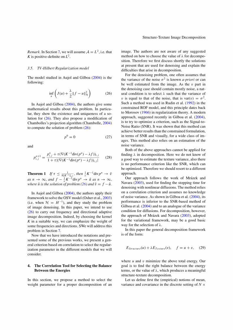
In Aujol and Gilboa (2004), the authors give somemathematical results about this problem. In particu-lar, they show the existence and uniqueness of a so-lution for (26). They also propose a modification ofChambolles’s projection algorithm (Chambolle, 2004)to compute the solution of problem (26):

p0 = 0 (27)

and

pn+1i, j = pn

i, j + τ (∇(K −1div(pn) − λ f ))i, j

1 + τ |(∇(K −1div(pn) − λ f ))i, j | (28)

Theorem 1 If τ ≤ 18‖K −1‖L2

, then 1λ

K −1divpn → v

as n → ∞, and f − 1λ

K −1divpn → u as n → ∞,where u is the solution of problem (26) and v = f − u.

In Aujol and Gilboa (2004), the authors apply theirframework to solve the OSV model (Osher et al., 2003)(i.e. when H = H−1), and they study the problemof image denoising. In this paper, we intend to use(26) to carry out frequency and directional adaptiveimage decomposition. Indeed, by choosing the kernelK in a suitable way, we can emphasize the weight ofsome frequencies and directions. SWe will address thisproblem in Section 7.

Now that we have introduced the notations and pre-sented some of the previous works, we present a gen-eral criterion based on correlation to select the regular-ization parameter in the different models that we willconsider.

4. The Correlation Tool for Selecting the BalanceBetween the Energies

In this section, we propose a method to select theweight parameter for a proper decomposition of an

image. The authors are not aware of any suggestedmethod on how to choose the value of λ for decompo-sition. Therefore we first discuss shortly the solutionsat present that are used for denoising and explain thedifficulties that arise in decomposition.

For the denoising problem, one often assumes thatthe variance of the noise σ 2 is known a-priori or canbe well estimated from the image. As the v part inthe denoising case should contain mostly noise, a nat-ural condition is to select λ such that the variance ofv is equal to that of the noise, that is var(v) = σ 2.Such a method was used in Rudin et al. (1992) in theconstrained ROF model, and this principle dates backto Morosov (1966) in regularization theory. A modernapproach, suggested recently in Gilboa et al. (2004),is to try to optimize a criterion, such as the Signal-to-Noise Ratio (SNR). It was shown that this method canachieve better results than the constrained formulation,in terms of SNR and visually, for a wide class of im-ages. This method also relies on an estimation of thenoise variance.

Both of the above approaches cannot be applied forfinding λ in decomposition. Here we do not know ofa good way to estimate the texture variance, also thereis no performance criterion like the SNR, which canbe optimized. Therefore we should resort to a differentapproach.

Our approach follows the work of Mrazek andNavara (2003), used for finding the stopping time fordenoising with nonlinear diffusions. The method relieson a correlation criterion and assumes no knowledgeof noise variance. As shown in Gilboa et al. (2004), itsperformance is inferior to the SNR-based method ofGilboa et al. (2004) and to an analogue of the variancecondition for diffusions. For decomposition, however,the approach of Mrazek and Navara (2003), adoptedfor the variational framework, may be a good basicway for the selection of λ.

In this paper the general decomposition frameworkis of the form:

EStructure(u) + λET exture(v), f = u + v, (29)

where u and v minimize the above total energy. Ourgoal is to find the right balance between the energyterms, or the value of λ, which produces a meaningfulstructure-texture decomposition.

Let us define first the (empirical) notions of mean,variance and covariance in the discrete setting of N ×

Aujol et al.

N pixels image. The mean is

q.= 1

N 2

∑1≤i, j≤N

qi, j ,

the variance is

V (q).= 1

N 2

∑1≤i, j≤N

(qi, j − q)2,

and the covariance is

cov(q, r ).= 1

N 2

∑1≤i, j≤N

(qi, j − q)(ri, j − r ).

We would like to have a measure that defines orthog-onality between two signals and is not biased by themagnitude (or variance) of the signals. A standard mea-sure in statistics is the correlation, which is the covari-ance normalized by the standard deviations of eachsignal:

corr(q, r ).= cov(q, r )√

V (q)V (r ).

By the Cauchy-Schwarz inequality it is not hardto see that cov(q, r ) ≤ √

V (q)V (r ) and therefore|corr(q, r )| ≤ 1. The upper bound 1 (completely cor-related) is reached for signals which are the same,up to an additive constant and up to a positive mul-tiplicative constant. The lower bound −1 (completelyanti-correlated) is reached for similar signals but witha negative multiplicative constant relation. When thecorrelation is 0 we refer to the two signals as not corre-lated. This is a necessary condition (but not a sufficientone) for statistical independence. It often implies thatthe signals can be viewed as produced by different“generators” or models.

To guide the parameter selection of a decompositionwe use the following assumption:

Assumption. The texture and the structure compo-nents of an image are not correlated.

This assumption can be relaxed by stating that thecorrelation of the components is very low. Let us de-fine the pair (uλ, vλ) as the one minimizing (29) for aspecific λ. As proved in Meyer (2001) for the TV − L2

model (and in Gilboa et al. (submitted) for any convex

structure energy term with L2, we have cov(uλ, vλ) ≥ 0for any non-negative λ and therefore

0 ≤ corr(uλ, vλ) ≤ 1, ∀λ ≥ 0. (30)

This means that one should not worry about nega-tive correlation values. Note that positive correlation isguaranteed in the TV − L2 case. As we will later see, inthe TV − L1 case we may have negative correlations,and should therefore be more careful.

Following the above assumption and the fact that thecorrelation is non-negative, to find the right parameterλ, we are led to consider the following problem:

λ∗ = argminλ (corr(uλ, vλ)) . (31)

In practice, one generates a scale-space using the pa-rameter λ (in our formulation, smaller λ means moresmoothing of u) and selects the parameter λ∗ as thefirst local minimum of the correlation function be-tween the structural part u and the oscillating part v.See also Gilboa et al. (submitted, 2003, 2005, Mrazekand Navara (2003), Aujol and Gilboa (2004) for relatedapproaches.

This selection method can be very effective in simplecases with very clear distinction between texture andstructure. In these cases corr(u, v) behaves smoothly,reaches a minimum approximately at the point wherethe texture is completely smoothed out from u, andthen increases, as more of the structure gets into thev part. See Figs. 1 to 5 in the next section for somenumerical examples. The graphs of corr(u, v) in the TV− L2 case behave quite as expected, and the selectedparameter lead to a good decomposition. We will makemore comments about the numerical results in the nextsection.

For more complicated images, there are textures andstructures of different scales and the distinction be-tween them is not obvious. In terms of correlation,there is no more a single minimum and the functionmay oscillate.

As a first approximation of a decomposition with asingle scalar parameter, we suggest to choose λ afterthe first local minimum of the correlation is reached.In some cases, a sharp change in the correlation is alsoa good indicator: after the correlation sharply dropsor before a sharp rise. At this stage we cannot claim afully automatic mechanism for the parameter selectionthat always works, but rather a highly relevant


measurement that should be taken into considerationin future development of automatic decompositions.

5. TV − L2 and TV − G Regularizations

In this section, we first show how we can use the cor-relation tool to select the parameter in the TV − L2

regularization model. We then show how we can ex-tend this method to the TV − G model.

5.1. Parameter Selection for the TV − L2 Model

Let us first recall here the TV − L2 problem (Rudin etal. 1992):

infu∈X

(J (u) + 1

2β‖ f − u‖2

L2

)(32)

We denote by (uβ, vβ ) the solution of (32). Thisregularization model has encountered a large success inimage denoising. One of the main reason of this successis that the total variation regularization preserve theedges of the restored image. It is straightforward toapply the correlation criterion of Section 4 to select theparameter in the TV − L2 model.

5.2. Parameter Selection for the TV − G Model

We focus here on the A2BC model (Aujol et al., 2005),which is a very good approximation. We show howwe can use the correlation criterion for the ROF model(Rudin et al. 1992) to carry out automatic image de-composition with the A2BC model. A first approachwould be to consider the correlation between u and v

computed with the A2BC algorithm. We have rejectedthis approach because of computation time: indeed, tocompute an accurate solution with the A2BC algorithmis about ten times slower than the classical TV − L2

minimization approach. We have decided instead to usethe mathematical connections between the ROF modeland the A2BC algorithm to select the parameter in amuch faster way.

To this end, we first need to give some mathematicalproperties of the A2BC model, (17), which is a wayto solve Meyer’s problem. As we have said in Sec-tion 3, the parameter α in (17) is set to a fixed smallvalue (α=1 in our numerical examples). The difficultyis to tune the µ parameter. We intend here to proposea method to compute automatically the parameter µ.

The idea is to use the method proposed for the ROFmodel in Section 5.1 (which is a straightforward appli-cation of the general method presented in Section 4).By choosing β as the first minimum of the functionβ �→ corr(uβ, vβ ) (where uβ is the solution of the ROFproblem (32) and vβ = f − uβ), we have an automaticalgorithm to compute the right parameter β for (32).All we need to do then is to relate the parameter β in(32) to µ in the A2BC model (17).

5.2.1. Relating β to µ. In Meyer (2001), Meyerintroduced the G norm to analyze the mathematicalproperties of the ROF model. As noticed in Stronget al. (2005), one of the main results of Meyer(2001) happens to be a straightforward corollary ofProposition 2:

Corollary 1. Let us denote by uβ the solution of (32),by vβ = f − uβ , and by f the mean of f.

• If ‖ f − f ‖G ≥ β, then ‖vβ‖G = ‖ f − uβ‖G = β.• If ‖ f − f ‖G ≤ β, then uβ = f .

As we can see, the behavior of the ROF model isclosely related to the G norm of the initial data f.

Lemma 1. The parameter β computed in Section 4is such that ‖vβ‖G = β.

Proof. Let us denote βmax = ‖ f − f ‖G . It is easy toshow that if β ∈ (0, βmax), then corr(uβ, vβ) remainsbounded. From Corollary 1, we get that if β ≥ βmax,then uβ = f and vβ = f − f . Therefore the first localminimum of the correlation is such that β ≤ βmax. Wethen conclude thanks to Corollary 1. �

Thanks to Section 5.1, we know how to computeautomatically the decomposition of an original imagewith the ROF model. And thanks to Lemma 1, we alsoknow the G norm of the v component we get with theROF model, i.e. ‖v‖G = β. As we have explained inthe introduction, Meyer’s idea is to replace the L2 normin the ROF model (32) by the G norm. The G normis better suited to capture oscillating patterns, such astextures, than the L2 norm (as it is numerically shownin Aujol and Chambolle (2005)). Therefore, a possi-ble improvement of the algorithm of Section 5.1 is tocompute Meyer’s decomposition under the constraintthat ‖v‖G = β. Since the G norm is a better choiceto capture the texture part of an image (Meyer, 2001;Aubert and Aujol, 2005; Aujol and Chambolle, 2005),

Aujol et al.

this would indeed gives a better decomposition resultthan the ROF model.

This naturally leads us to consider the A2BC model(17) with

µ = β (33)

Indeed, with such a parameter, the v component com-puted with the A2BC model is such that ‖v‖G ≤ β.And we prove in the following subsection that in factwe have ‖v‖G = β.

5.2.2. Some Mathematical Results About the A2BCModel. The functional to minimize in (17) is the fol-lowing:

F(u, v) = J (u)+ J ∗(

v

µ

)+ 1

2α‖ f −u −v‖2

L2 (34)

The following Lemma is proved in Aujol et al.(2005):

Lemma 2. There exists a unique couple (u, v) ∈ X ×Gµ minimizing F on X × X.

From now on, let us denote by (u, v) the uniquesolution of the A2BC problem (17). The next resultwill help to see the connection between the parameterβ in the ROF model and the parameter µ in the A2BCalgorithm:

Proposition 3. The following alternative holds:

• If ‖ f − f ‖G ≤ µ, then v = f − f .• If ‖ f − f ‖G ≥ µ, then ‖v‖G = µ.

Proof. Let us first remark that F(u, v) ≥ 0 for all(u, v) in X × X . Moreover, if we assume that ‖ f −f ‖G ≤ µ, we have F( f , f − f ) = 0, which meansthat ( f , f − f ) is a minimizer of F. We then get thefirst point of Proposition 3 thanks to the uniquenessresult of Lemma 2.

We now turn our attention to the second point ofProposition 3. We therefore assume that ‖ f − f ‖G ≥µ. Let us consider the following function defined onX × X :

H (u, v) = J (u) + 1

2α‖ f − u − v‖2

L2 (35)

H is a proper convex continuous function defined onX×X . There exists therefore (u, v) in X×Gµ such that(u, v) is a minimizer of H on X×Gµ. Let us remark thatH ( f , f − f ) = 0. We then consider the function g :t �→ ‖t v+(1− t)( f − f )‖G . g is a continuous functionon [0,1]. Moreover, we have g(0) = ‖ f − f ‖G ≥ µ

and g(1) = ‖v‖G ≤ µ. There exists thus t in [0, 1] suchthat g(t) = ‖t v+ (1− t)( f − f )‖G = µ. Let us denoteby v = t v + (1 − t)( f − f ) and u = t u + (1 − t) f .Since H is a convex function, we get that H (u, v) ≤t H (u, v)+(1−t)H ( f , f − f ) ≤ H (u, v). We thereforededuce that (u, v) is a minimizer of H on X ×Gµ. SinceH and F coincide on X × Gµ, we get that (u, v) is aminimizer of F on X × X . From Lemma 2, we thenconclude that (u, v) = (u, v) the unique minimizer ofF on X × X , and ‖v‖G = ‖v‖G = µ. �

From Lemma 1 and Corollary 1, we know that ‖ f −f ‖G ≥ β. And from (33), we have β = µ. FromProposition 3, we thus deduce that v, the v componentwe get with the A2BC algorithm, is such that ‖v‖G = µ.This new v component has therefore the same G normas the one of the v component (vβ) computed with theROF model in Section 5.1. But since the G norm isbetter at capturing the oscillating patterns then the L2

norm, this new decomposition is more accurate thanthe previous one.

This analysis is confirmed by the numerical resultswe get in the next subsection.

5.3. Numerical Results

Let us first summarize the method we propose to com-pute the decomposition into geometry and texture withthe A2BC model.

Automatic algorithm for the A2BC model:

1. Set α = 1 in (17).2. Compute β as the first minimum of the function

β �→ corr(uβ, vβ ) (where uβ is the solution of theROF problem (32) and vβ = f − uβ).

3. Set µ = β in (17).4. Compute the decomposition with the algorithm

(21)–(23).

We show some numerical results in Figs. 1–5 of TV− L2 and TV − G decompositions. As expected, theresults obtained with the A2BC algorithm are slightlybetter than the ones obtained with the ROF model. For


Figure 1. A simple example.

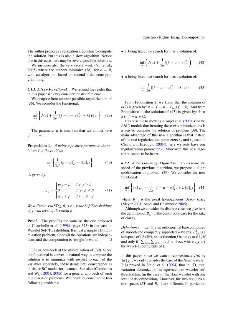
instance, on Fig. 1, one can check that the square isless eroded with Meyer’s G norm (and in this case, thesquare is a geometrical feature and should remain inthe u component). On Fig. 5, one sees that the leg of thetable appears much more in the v component with theROF model than with the A2BC algorithm. In general,the ROF model already does a good job, and the A2BCalgorithm seems to bring a small improvement. Noticethat we do not claim that we compute the best possibleresults (see Vese and Osher, 2003; Osher et al., 2003;Aujol et al., 2005; Aujol and Chambolle, 2005) forinstance where the parameters are tuned manually):what we claim is that our parameter selection methodleads to a visually good result (for both models).

Detailed explanation on the correlation graph: Inthese experiments the correlation corr(u, v) of 50 val-ues of λ is plotted. We initially set λ0 = 1 and re-duced each time the value by a factor of 0.9 suchthat λn+1 = 0.9λn . To solve the minimization prob-lem for λn+1 we initialized with the solution obtainedfor λn , and therefore the convergence is quite fast. Alsonote that in practice one needs not compute the whole

Figure 2. A synthetic image.

Figure 3. Barbara image and TV − L2 correlation graph.

graph and can stop when the first local minimum isreached. One may also use courser λ resolutions to savesome computational efforts. Note that the correlationgraph finds well the right splitting parameter in Figs.1 and 2 and even in the more complex Barbara image,Figs. 3–5. In these cases a fully automatic decomposi-tion is possible. In all the correlation graphs the split-ting point chosen by our automatic algorithm is markedwith “x”.

Aujol et al.

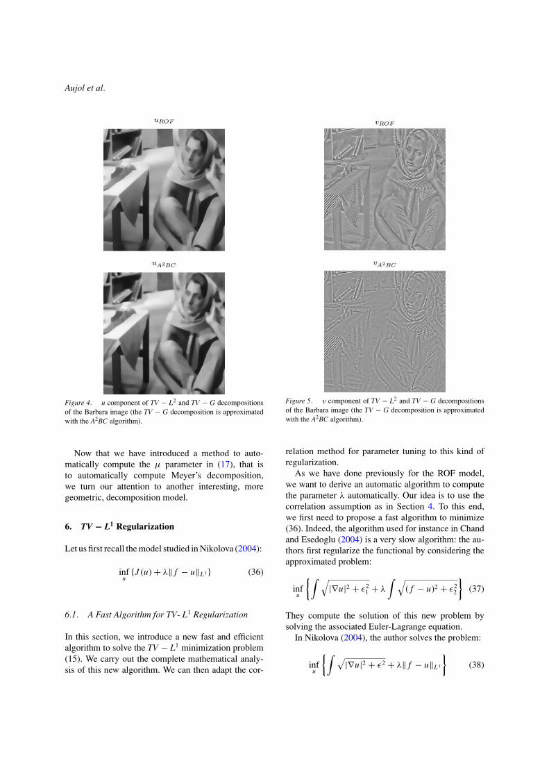
Figure 4. u component of TV − L2 and TV − G decompositionsof the Barbara image (the TV − G decomposition is approximatedwith the A2BC algorithm).

Now that we have introduced a method to auto-matically compute the µ parameter in (17), that isto automatically compute Meyer’s decomposition,we turn our attention to another interesting, moregeometric, decomposition model.

6. TV − L1 Regularization

Let us first recall the model studied in Nikolova (2004):

infu

{J (u) + λ‖ f − u‖L1} (36)

6.1. A Fast Algorithm for TV- L1 Regularization

In this section, we introduce a new fast and efficientalgorithm to solve the TV − L1 minimization problem(15). We carry out the complete mathematical analy-sis of this new algorithm. We can then adapt the cor-

Figure 5. v component of TV − L2 and TV − G decompositionsof the Barbara image (the TV − G decomposition is approximatedwith the A2BC algorithm).

relation method for parameter tuning to this kind ofregularization.

As we have done previously for the ROF model,we want to derive an automatic algorithm to computethe parameter λ automatically. Our idea is to use thecorrelation assumption as in Section 4. To this end,we first need to propose a fast algorithm to minimize(36). Indeed, the algorithm used for instance in Chandand Esedoglu (2004) is a very slow algorithm: the au-thors first regularize the functional by considering theapproximated problem:

infu

{∫ √|∇u|2 + ε2

1 + λ

∫ √( f − u)2 + ε2

2

}(37)

They compute the solution of this new problem bysolving the associated Euler-Lagrange equation.

In Nikolova (2004), the author solves the problem:

infu

{∫ √|∇u|2 + ε2 + λ‖ f − u‖L1

}(38)


The author proposes a relaxation algorithm to computethe solution, but this is also a slow algorithm. Noticethat in this case there may be several possible solutions.

We mention also the very recent work (Yin et al.,2005) where the authors minimize (38), for ε = 0,with an algorithm based on second order cone pro-gramming.

6.1.1. A New Functional. We remind the reader thatin this paper we only consider the discrete case.

We propose here another possible regularization of(36). We consider the functional:

infu,v

{J (u) + 1

2α‖ f − u − v‖2

L2 + λ‖v‖L1

}(39)

The parameter α is small so that we almost havef = u + v.

Proposition 4. β being a positive parameter, the so-lution V of the problem

infv

{1

2β‖g − v‖2

L2 + ‖v‖L1

}(40)

is given by:

vi, j =

gi, j − β if gi, j ≥ β

0 if |gi, j | ≤ β

gi, j + β if gi, j ≤ −β

(41)

We will write v = ST(g, β), i.e. v is the Soft Thresholdingof g with level of threshold β.

Proof. The proof is the same as the one proposedin Chambolle et al. (1998) (page 323) in the case ofWavelet Soft Thresholding. It is just a simple 1D mini-mization problem, since all the equations are indepen-dent, and the computation is straightforward. �

Let us now look at the minimization of (39). Sincethe functional is convex, a natural way to compute thesolution is to minimize with respect to each of thevariables separately, and to iterate until convergence asin the A2BC model for instance. See also (Combettesand Wajs 2004; 2005) for a general approach of suchminimization problems. We therefore consider the twofollowing problems:


infu

(J (u) + 1

2α‖ f − u − v‖2

L2

)(42)


infv

1

2α‖ f − u − v‖2

L2 + λ‖v‖L1 (43)

From Proposition 2, we know that the solution of(42) is given by: u = f − v − PGα

( f − v). And fromProposition 4, the solution of (43) is given by: v =ST ( f − u, αλ).

It is possible to show as in Aujol et al. (2005) (for theA2BC model) that iterating these two minimizations isa way to compute the solution of problem (39). Themain advantage of this new algorithm is that insteadof the two regularization parameters ε1 and ε2 used inChand and Esedoglu (2004), here we only have oneregularization parameter λ. Moreover, this new algo-rithm seems to be faster.

6.1.2. A Thresholding Algorithm. To increase thespeed of the previous algorithm, we propose a slightmodification of problem (39). We consider the newfunctional:

infu,v

{‖u‖B1

1,1+ 1

2α‖ f − u − v‖2

L2 + λ‖v‖L1

}(44)

where B11,1 is the usual homogeneous Besov space

(Meyer 2001; Aujol and Chambolle 2005).Although we consider the discrete case, we give here

the definition of B11,1 in the continuous case for the sake

of clarity.

Definition 3. Let � j,k an orthonormal base composedof smooth and compactly supported wavelets. B1

1,1 is asubspace of L2 (R2), and a function f belongs to B1

1,1 ifand only if:

∑j∈Z

∑k∈Z2 |c j,k | < +∞, where cj,k are

the wavelet coefficients of f.

In this paper, since we want to approximate J(u) by‖u‖B1

1,1, we only consider the case of the Haar wavelet.

It is proved in Steidl et al. (2004) that in 1D, totalvariation minimization is equivalent to wavelet softthresholding (in the case of the Haar wavelet with onelevel of decomposition). However, the two regulariza-tion spaces (BV and B1

1,1) are different. In particular,

Aujol et al.

characteristic functions of sets with finite perimeter be-long to BV but are not in B1

1,1. This is the reason whyit can be expected that the edges of the original imagef are better put in the geometrical component u withmodel (39) than with (44).

Let us now look at the minimization of (44). Weadopt the same strategy as for solving (39), that is weminimize with respect to each of the variables sepa-rately. We therefore consider the two following prob-lems:


infu

(‖u‖B1

1,1+ 1

2α‖ f − u − v‖2

L2

)(45)


infv

1

2α‖ f − u − v‖2

L2 + λ‖v‖L1 (46)

From Chambolle et al. (1998), we know that thesolution of (45) is given by: u = W ST ( f − v, α),where W ST ( f − v, α) stands for the Wavelet SoftThresholding of f-v with threshold α (Meyer, 2001;Aujol and Chambolle, 2005). And from Proposition,the solution of (46) is given by:v = ST ( f − u, αλ),where ST ( f −u, αλ) stands for the Soft Thresholdingof f-u with threshold αλ

The advantage for having replaced J(u) by ‖u‖B11,1

is that now, to minimize the new functional (44), wejust need to iterate thresholding schemes. This is whythe following algorithm is a very fast one (much fasterthan the one used in Chand and Esedoglu (2004) forinstance).

Algorithm:

1. Initialization:

u0 = v0 = 0 (47)

2. Iterations:

vn+1 = ST ( f − un, αλ) (48)

un+1 = W ST ( f − vn+1, α) (49)

3. Stopping test: we stop if

max(|un+1 − un|, |vn+1 − vn|) ≤ ε (50)

6.1.3. Mathematical Analysis. We now show somemathematical results about our new model, and weprove the convergence of the algorithm. We will usethe notation:

M(u, v) = ‖u‖B11,1

+ 1

2α‖ f −u−v‖2

L2 +λ‖v‖L1 (51)

Theorem 2. Problem (44) admits a unique solution(u, v) in (X × X).

Proof. See Appendix A.1.. �

The next result is a consequence of Theorem 2:

Proposition 5. The sequence (un, vn) built in (47)–(49) converges to the unique minimizer of problem (44).


The next result shows that when α goes to 0, thenthe solution of problem (44) goes to a solution of theproblem:

infu

(‖u‖B11,1

+ λ‖ f − u‖L1

)(52)

Proposition 6. Let us fix λ >0 in (52). We considerαn a decreasing sequence in R+∗ such that αn → 0.Let us denote by (uαn , vαn ) the solution of problem(44). Then the sequence (uαn , vαn ) is bounded, and anycluster point is of the form (u0, f − u0) with u0 solutionof problem (52).


Remark. It is easy to show that problem (52) has asolution (the functional is convex and coercive). In thecase when problem (52) has a unique solution u0, thenthe sequence ((uαn , vαn ) converges to $(u0, f − u0).


A main difference with the classical TV − L2 approach(Rudin et al., 1992) is that with the TV − L1 model, thev component is not constrained to be of zero mean (nu-merical experiments show that indeed the mean valuechanges for different values of λ and is not necessarilyclose to zero).


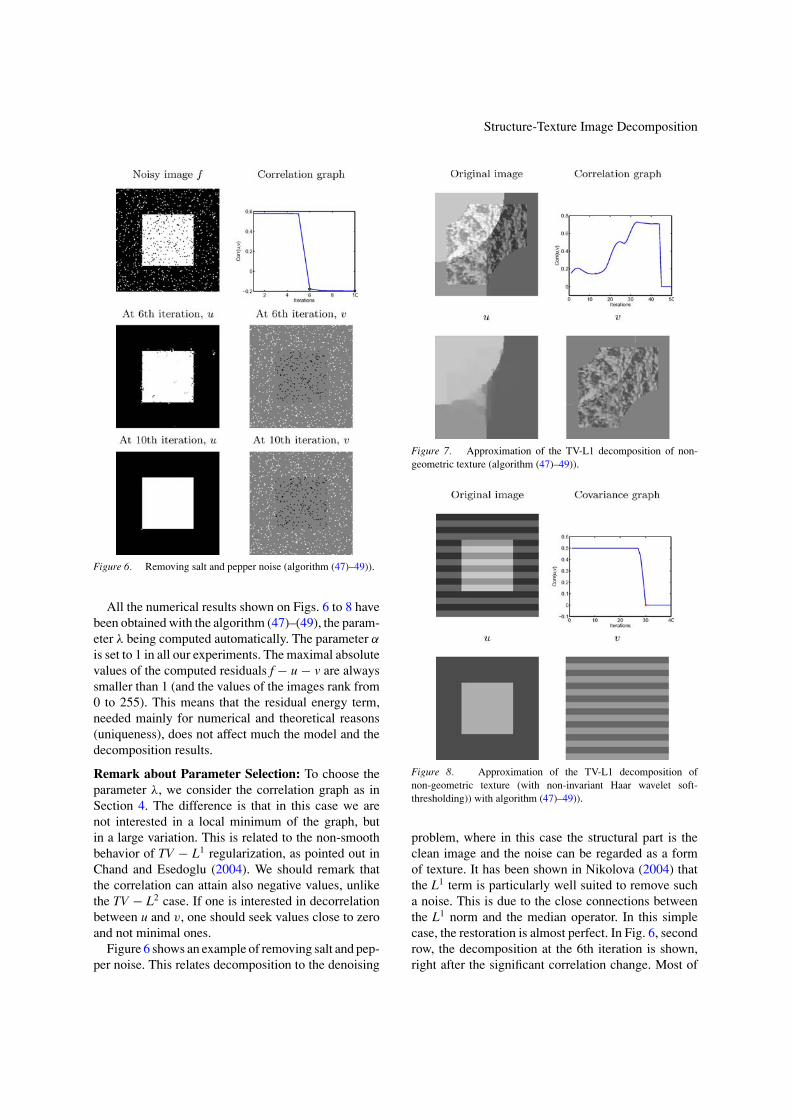
Figure 6. Removing salt and pepper noise (algorithm (47)–49)).

All the numerical results shown on Figs. 6 to 8 havebeen obtained with the algorithm (47)–(49), the param-eter λ being computed automatically. The parameter α

is set to 1 in all our experiments. The maximal absolutevalues of the computed residuals f − u − v are alwayssmaller than 1 (and the values of the images rank from0 to 255). This means that the residual energy term,needed mainly for numerical and theoretical reasons(uniqueness), does not affect much the model and thedecomposition results.

Remark about Parameter Selection: To choose theparameter λ, we consider the correlation graph as inSection 4. The difference is that in this case we arenot interested in a local minimum of the graph, butin a large variation. This is related to the non-smoothbehavior of TV − L1 regularization, as pointed out inChand and Esedoglu (2004). We should remark thatthe correlation can attain also negative values, unlikethe TV − L2 case. If one is interested in decorrelationbetween u and v, one should seek values close to zeroand not minimal ones.

Figure 6 shows an example of removing salt and pep-per noise. This relates decomposition to the denoising

Figure 7. Approximation of the TV-L1 decomposition of non-geometric texture (algorithm (47)–49)).

Figure 8. Approximation of the TV-L1 decomposition ofnon-geometric texture (with non-invariant Haar wavelet soft-thresholding)) with algorithm (47)–49)).

problem, where in this case the structural part is theclean image and the noise can be regarded as a formof texture. It has been shown in Nikolova (2004) thatthe L1 term is particularly well suited to remove sucha noise. This is due to the close connections betweenthe L1 norm and the median operator. In this simplecase, the restoration is almost perfect. In Fig. 6, secondrow, the decomposition at the 6th iteration is shown,right after the significant correlation change. Most of

Aujol et al.

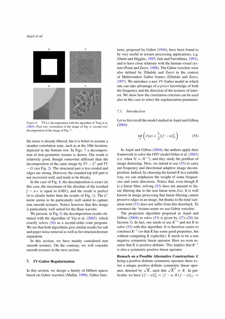
Figure 9. TV-L1 decomposition with the algorithm of Ying et al.(2005). First row: restoration of the image of Fig. 6; second row:decomposition of the image of Fig. 7.

the noise is already filtered, but it is better to assume asteadier correlation state, such as at the 10th iteration,depicted in the bottom row. In Figs. 7 a decomposi-tion of non-geometric texture is shown. The result isrelatively good, though somewhat different than thedecomposition of the same image by TV − L2 and TV− G (see Fig. 2). The structural part is less eroded andedges are strong. However, the rounded top left part isnot recovered well, and tends to be blocky.

In the case of Fig. 8, the decomposition is exact (inthis case, the maximum of the absolute of the residualf − u-v is equal to 0.001), and the result is perfect(it is clearly better than the results of Fig. 1). The L1

norm seems to be particularly well suited to capturenon smooth textures. Notice however that this imageis particularly well suited for the Haar wavelet.

We present, in Fig. 9, the decomposition results ob-tained with the algorithm of Yin et al. (2005), whichexactly solves (36) as a second-order cone program.We see that both algorithms give similar results for saltand peper noise removal as well as for structure/textureseparation.

In this section, we have mainly considered nonsmooth textures. On the contrary, we will considersmooth textures in the next section.

7. TV-Gabor Regularization

In this section, we design a family of Hilbert spacesbased on Gabor wavelets (Mallat, 1998). Gabor func-

tions, proposed by Gabor (1946), have been found tobe very useful in texture processing applications, e.g.(Dunn and Higgins, 1995; Jain and Farrokhnia, 1991),and to have close relations with the human-visual sys-tem (Porat and Zeevi, 1988). The Gabor wavelets werealso defined by Zibulski and Zeevi in the contextof Multiwindow Gabor frames (Zibulski and Zeevi,1997). We introduce a new TV-Gabor model in whichone can take advantage of a-priori knowledge of boththe frequency and the direction of the textures of inter-est. We show how the correlation criterion can be usedalso in this case to select the regularization parameter.

7.1. Introduction

Let us first recall the model studied in Aujol and Gilboa(2004):

infu

(J (u) + λ

2‖ f − u‖2

H

)(53)

In Aujol and Gilboa (2004), the authors apply theirframework to solve the OSV model Osher et al. (2003)(i.e. when H = H−1), and they study the problem ofimage denoising. Here, we intend to use (53) to carryout frequency and directional adaptive image decom-position. Indeed, by choosing the kernel K in a suitableway, we can emphasize the weight of some frequen-cies and some directions. Notice that, even though Kis a linear filter, solving (53) does not amount to lin-ear filtering due to the non linear term J(u). It is wellknown in image processing that linear filtering cannotpreserve edges in an image, but thanks to the total vari-ation term (53) does not suffer from this drawback. Toconstruct the “texture-norm we use Gabor wavelets.

The projection algorithm proposed in Aujol andGilboa (2004) to solve (53) is given by (27)–(28) (inSection 3). In fact, one needs to use K−1 and not K tosolve (53) with this algorithm. It is therefore easier toconstruct K−1 (so that K has some good properties, butwithout computing K explicitly). K needs to be a nonnegative symmetric linear operator. Here we even as-sume that K is positive-definite. This implies that K−1

is also a symmetric positive linear operator.

Remark on a Possible Alternative Construction: Kbeing a positive-definite symmetric operator, there ex-ists a unique positive-definite symmetric linear oper-ator, denoted by

√K , such that

√K

2 = K . In par-ticular, we have ‖ f − u‖2

H = 〈 f − u, K ( f − u)〉L2 =


Figure 10. The kernel K and its inverse K−1 for the OSV, ROFand the proposed TV-Gabor model.

‖√K ( f −u)‖2L2 . We can then rewrite problem (53) as:

infu

(J (u) + λ

2‖√

K ( f − u)‖2L2

)(54)

In fact, instead of K−1, it also may be interesting toconstruct

√K

−1. In what follows, we only focus on

K−1, but our construction can be applied to√

K−1

aswell.

7.2. Texture-specific Kernels

In Aujol and Gilboa (2004) it was shown that the differ-ence between the OSV model (Osher et al., 2003) andROF model (Rudin et al., 1992) could be understood asfrequency weighting of the L2 norm for the H−1 fidelityterm of OSV. The frequency weighting of the squarenorm is proportional to 1

ω2 , which corresponds to the−1 operator in the frequency domain, see Fig. 10. Thelow frequencies are therefore highly penalized in thefidelity term, considerably reducing the eroding effectcompared with ROF. This has proved to be an efficient

tool for image denoising (Osher et al., 2003; Aujol andChambolle 2005). In Aujol and Gilboa (2004) it wassuggested that other linear kernels could be used foradaptive frequency algorithms.

In this section we address the problem of designinga family of kernels for image decomposition. The op-erator K is a convolution operator, therefore K−1 in theFourier domain is simply its inverse. Moreover, K−1 isalso a convolution operator. We denote by H the asso-ciated filter, and in the rest of the section we focus onthe designing of this filter.

In the u+v decomposition model K penalizes fre-quencies that are not considered as part of the texturecomponent. Therefore K−1 could be interpreted as thefrequencies which should mainly be included in thetexture part. A general and simple characterization oftextures could be done using Gabor functions. Thesefunctions would typically describe the type of textureswe would like to extract. Naturally, they apply as goodcandidates for K−1. As already mentioned, the inversekernel is actually the one needed in the numerical im-plementation. Thus our proposed design strategy is touse Gabor functions for constructing the inverse ker-nel. Notice that other design methods could be used.We use the function:

g(x) = cos (2πνx)1√

2πσ 2exp

(−x2

2σ 2

)(55)

This gives the following values for the filter H:

hk = cos (2πνk)1√

2πσ 2exp

(−k2

2σ 2

)(56)

v ∈ (0, 0.5] is the frequency of the texture. σ is relatedto the width of the band-pass around this frequency. Asmall σ in the spatial domain means a wide band-passin the frequency domain. If we know the frequencyof the texture we want to get, it is then interesting touse a large σ (which means a small band-pass in thefrequency domain). Note that some restrictions applyfor choosing σ , see Lemma 4. Actually, σ cannot bevery large, which may be interpreted as a from of anuncertainty principle.

Equation (55) is a one dimension filter. There aremany methods to then design a 2D filter. One pos-sibility is to consider the product g(x)g(y). We willanalyze this possibility later. Another choice to con-struct our filter H is to use rotationally invariant Gabor

Aujol et al.

wavelets as:

g(x, y) = cos(

2πν√

x2 + y2) 1√

2πσ 2

× exp

(−x2 − y2

2σ 2

)(57)

Such a choice will give better numerical results whenthe texture is known to be rotationally invariant.

Directions: Many textures are not rotationally in-variant. It is therefore interesting to add this directioninformation in our filter H. To do so, we just need touse a 1D filter as (55), and then rotate it so that it fitsthe direction of the texture. A possible improvementis to use an ellipse (see Dunn and Higgins (1995) forinstance).

7.3. 1D and 2D filters

In this subsection, we propose a way to construct a 2Dkernel K−1 (in fact of the associated filter H) out of a1D filter:

Hx =(

h d−12

, . . . , h1, h0, h1, . . . , h d−12

)(58)

where d is the dimension of the filter Hx, and hk is givenby (56). Since K−1 is symmetric, we also choose Hx tobe symmetric. We then set H = Hx∗Hy , where H standsfor the filter associated to K−1, ∗ denotes convolution,and Hy = Hx

T , where T stands for transpose.

Remark. In all this section, for the convolution, weconsider periodic boundary conditions.

7.4. Eigenvalues

In this subsection, we compute the eigenvalues of K−1,and give a sufficient condition so that they are positive.

The filter H associated with K−1 should define alinear symmetric positive operator. By construction,H defines a linear symmetric operator. But as we willsee, we have to impose some conditions on the valueshk of the filter so that it is positive. We recall that alinear symmetric operator is positive if and only ofits eigenvalues are positive (this can even be takenas a definition). To get the positivity for H, we aretherefore lead to compute its associated eigenvalues(the ones of the associated linear mapping). Since we

have constructed H out of two 1-D filters, we are infact interested in the eigenvalues of these filters (sincethey will give us the eigenvalues of K−1). Since K−1

is positive, we also impose the constraint that Hx ispositive.

The filtering of an image of size N × M by Hx

corresponds to a linear mapping from RNM to R

NM

(this is the reason why we speak of the eigenvalues ofthe filter H, which are in fact the eigenvalues of thecorresponding linear mapping). Let us denote by Ax

(resp Ay) the matrix of size (NM)2 associated to Hx

(resp Hy). An image I is a matrix (Ii,j), with 1 ≤ i ≤ Nand 1 ≤ j ≤ M. We rewrite it as a 1 Dimensional vectorIk, with 1 ≤ k ≤ NM, using Ik=Ii,j if k=M(i-1)+j.

Since Ax and Ay have a very particular form (theyare both circulant matrices), we can compute the exactvalues of their eigenvalues, as stated by the followingresult:

Proposition 7. The eigenvalues of Ax are:

h0 + 2

d−12∑

k=1

hk cos

(2πqk

M

), 0 ≤ q ≤ M

2

(59)

and the ones of Ay are:

h0 + 2

d−12∑

k=1

hk cos

(2πqk

N

), 0 ≤ q ≤ N

2

(60)

Proof. The proof is just a consequence of the fact thatAx and Ay are circulant matrix. We refer the interestedreader to Aujol et al. (2005) for the details. �

Now that we have computed the eigenvalues of Ax

and Ay, we can get the ones of K−1. Since Ax and Ay

commute, the eigenvalues of K−1 are contained in theset:{

P1(ω

pM

)P2

(ω

qN

), 0 ≤ q ≤ M

2, 0 ≤ q ≤ N

2

}(61)

Since the eigenvalues of Ax and Ay are positive, soare the ones of K−1. If we denote by γ x

min (resp γy

min) thesmallest eigenvalue of Ax (resp Ay) and by γ x

max (respγ

ymax) the largest eigenvalue of Ax (resp Ay), then, if γ

is an eigenvalue of K−1, we have:

γ xminγ

ymin ≤ γ ≤ γ x

maxγy

max (62)


From this last point, we deduce in particular that

‖K −1‖L2 ≤ γ xmaxγ

ymax (63)

Lemma 3. If we choose τ ≤ 18γ x

maxγy

maxin algorithm

(28), then the algorithm converges.

Proof. This a direct consequence of (63) and ofTheorem 1 (in Section 3). �

Unfortunately, the eigenvalues of K−1 can be neg-ative. The next lemma gives a sufficient condition forthe eigenvalues of K−1 to be positive.

Lemma 4. If

h0 ≥ 2

d−12∑

k=1

|hk | (64)

then the eigenvalues of Ax, Ay and K−1 are positive.

Proof. This is a consequence of Proposition 7 and of(61). �

Notice that (64) is only a sufficient condition. Theeigenvalues can still be positive in less restrictive cases,and can be computed explicitly for the designed kernel(see Proposition 7).

By using Lemma 4 and the explicit values of hk

given by (56), we can derive more explicit sufficientconditions about the positivity of the eigenvalues ofK−1. In particular, we show that if σ is small enough,then the eigenvalues of H are positive, see more detailsin Aujol and Gilboa (2005).


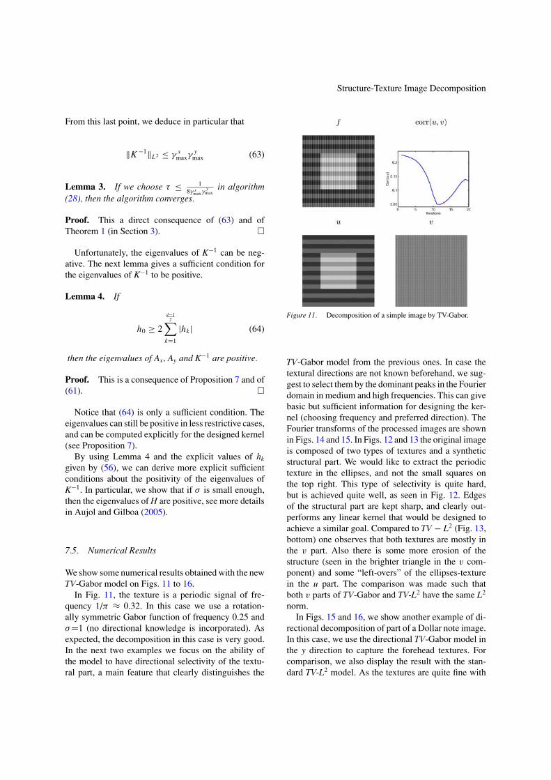
We show some numerical results obtained with the newTV-Gabor model on Figs. 11 to 16.

In Fig. 11, the texture is a periodic signal of fre-quency 1/π ≈ 0.32. In this case we use a rotation-ally symmetric Gabor function of frequency 0.25 andσ=1 (no directional knowledge is incorporated). Asexpected, the decomposition in this case is very good.In the next two examples we focus on the ability ofthe model to have directional selectivity of the textu-ral part, a main feature that clearly distinguishes the

Figure 11. Decomposition of a simple image by TV-Gabor.

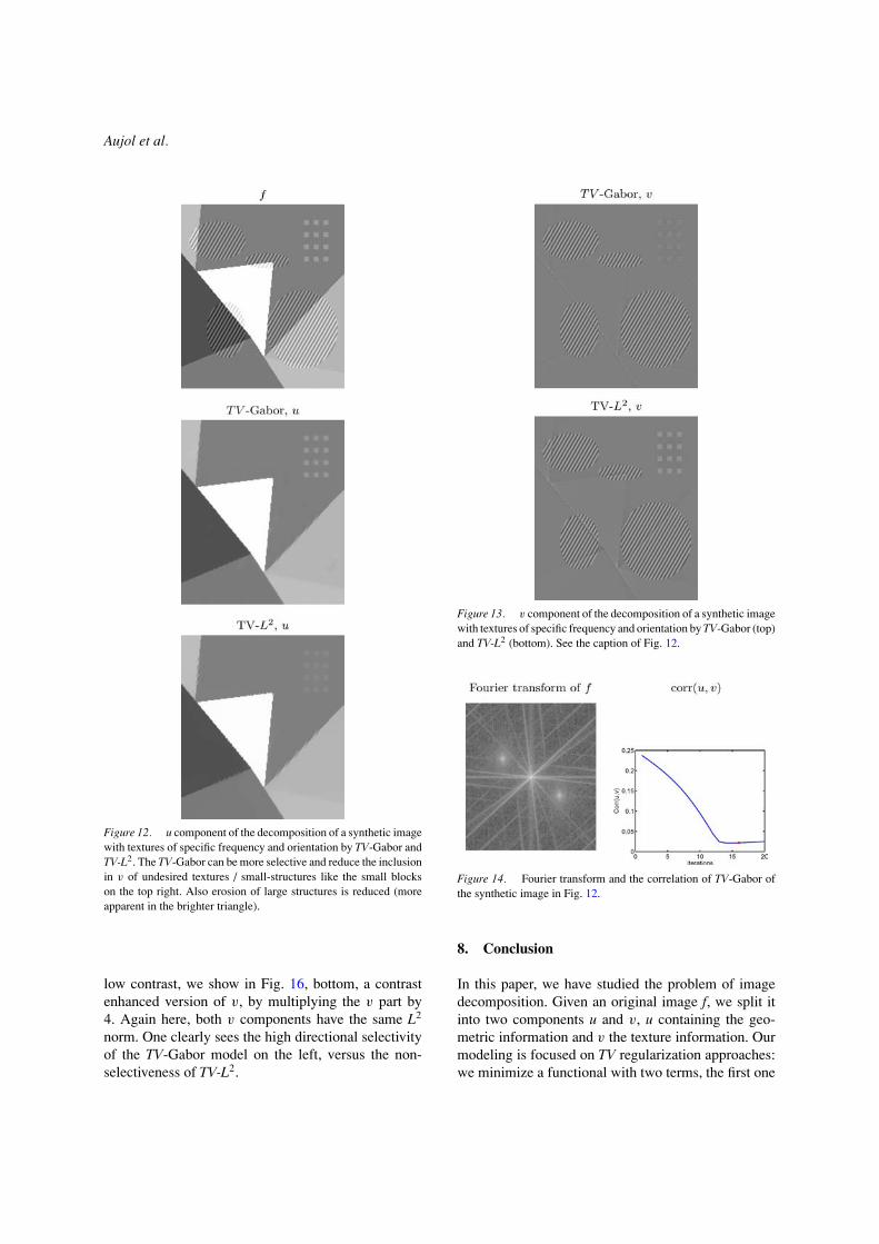
TV-Gabor model from the previous ones. In case thetextural directions are not known beforehand, we sug-gest to select them by the dominant peaks in the Fourierdomain in medium and high frequencies. This can givebasic but sufficient information for designing the ker-nel (choosing frequency and preferred direction). TheFourier transforms of the processed images are shownin Figs. 14 and 15. In Figs. 12 and 13 the original imageis composed of two types of textures and a syntheticstructural part. We would like to extract the periodictexture in the ellipses, and not the small squares onthe top right. This type of selectivity is quite hard,but is achieved quite well, as seen in Fig. 12. Edgesof the structural part are kept sharp, and clearly out-performs any linear kernel that would be designed toachieve a similar goal. Compared to TV − L2 (Fig. 13,bottom) one observes that both textures are mostly inthe v part. Also there is some more erosion of thestructure (seen in the brighter triangle in the v com-ponent) and some “left-overs” of the ellipses-texturein the u part. The comparison was made such thatboth v parts of TV-Gabor and TV-L2 have the same L2

norm.In Figs. 15 and 16, we show another example of di-

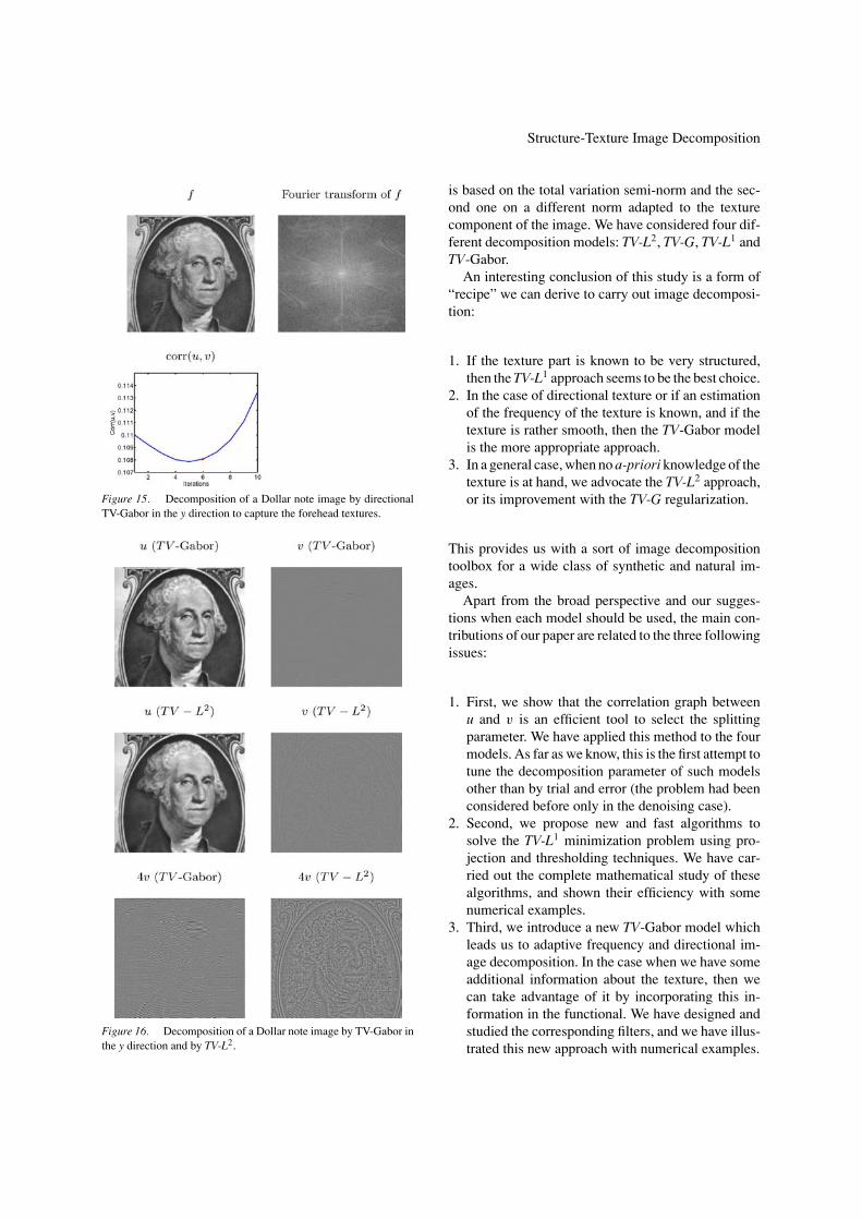
rectional decomposition of part of a Dollar note image.In this case, we use the directional TV-Gabor model inthe y direction to capture the forehead textures. Forcomparison, we also display the result with the stan-dard TV-L2 model. As the textures are quite fine with

Aujol et al.

Figure 12. u component of the decomposition of a synthetic imagewith textures of specific frequency and orientation by TV-Gabor andTV-L2. The TV-Gabor can be more selective and reduce the inclusionin v of undesired textures / small-structures like the small blockson the top right. Also erosion of large structures is reduced (moreapparent in the brighter triangle).

low contrast, we show in Fig. 16, bottom, a contrastenhanced version of v, by multiplying the v part by4. Again here, both v components have the same L2

norm. One clearly sees the high directional selectivityof the TV-Gabor model on the left, versus the non-selectiveness of TV-L2.

Figure 13. v component of the decomposition of a synthetic imagewith textures of specific frequency and orientation by TV-Gabor (top)and TV-L2 (bottom). See the caption of Fig. 12.

Figure 14. Fourier transform and the correlation of TV-Gabor ofthe synthetic image in Fig. 12.

8. Conclusion

In this paper, we have studied the problem of imagedecomposition. Given an original image f, we split itinto two components u and v, u containing the geo-metric information and v the texture information. Ourmodeling is focused on TV regularization approaches:we minimize a functional with two terms, the first one


Figure 15. Decomposition of a Dollar note image by directionalTV-Gabor in the y direction to capture the forehead textures.

Figure 16. Decomposition of a Dollar note image by TV-Gabor inthe y direction and by TV-L2.

is based on the total variation semi-norm and the sec-ond one on a different norm adapted to the texturecomponent of the image. We have considered four dif-ferent decomposition models: TV-L2, TV-G, TV-L1 andTV-Gabor.

An interesting conclusion of this study is a form of“recipe” we can derive to carry out image decomposi-tion:

1. If the texture part is known to be very structured,then the TV-L1 approach seems to be the best choice.

2. In the case of directional texture or if an estimationof the frequency of the texture is known, and if thetexture is rather smooth, then the TV-Gabor modelis the more appropriate approach.

3. In a general case, when no a-priori knowledge of thetexture is at hand, we advocate the TV-L2 approach,or its improvement with the TV-G regularization.

This provides us with a sort of image decompositiontoolbox for a wide class of synthetic and natural im-ages.

Apart from the broad perspective and our sugges-tions when each model should be used, the main con-tributions of our paper are related to the three followingissues:

1. First, we show that the correlation graph betweenu and v is an efficient tool to select the splittingparameter. We have applied this method to the fourmodels. As far as we know, this is the first attempt totune the decomposition parameter of such modelsother than by trial and error (the problem had beenconsidered before only in the denoising case).

2. Second, we propose new and fast algorithms tosolve the TV-L1 minimization problem using pro-jection and thresholding techniques. We have car-ried out the complete mathematical study of thesealgorithms, and shown their efficiency with somenumerical examples.

3. Third, we introduce a new TV-Gabor model whichleads us to adaptive frequency and directional im-age decomposition. In the case when we have someadditional information about the texture, then wecan take advantage of it by incorporating this in-formation in the functional. We have designed andstudied the corresponding filters, and we have illus-trated this new approach with numerical examples.

Aujol et al.

In this paper we presented a way to design simpletexture-specific filters based on Gabor functions. Other,more sophisticated methods could be incorporated tothis framework, such as ones based on wavelets (Starcket al., 2003). In future works we intend to explore theseissues. Notice that a straightforward extension of thenew TV-Gabor model to multiple selected directions,is to use the linearity of the Hilbert fitting term andsimply add several directional kernels.

A natural generalization for the u+v decompositionis to consider a multi-scale approach, as done inTadmor et al. (2004), Gilboa et al. (2003, submitted),Osher et al. (2004), and Groetsch and Scherzer(2001). This also relates to the parameter selectionproblem, where better and more accurate mechanismscould be used instead of the correlation criterion. Amore detailed version of this work, with some moretheoretical results and proofs can be found in ourreport (Aujol and Gilboa, 2004).

Appendix A: Proofs for the TV − L1 Algorithm

In this appendix, we give the proofs of the Mathemati-cal results stated in Section 6 for the new fast TV − L1

algorithm.

A.1. Existence and Uniqueness of a Solution

We give here the proof of Theorem 2 stated in Section 6.We first recall the theorem:

Theorem 2. Problem (44) admits a unique solution(u, v) in (X × X).

To prove Theorem 2, we will use the followinglemma:

Lemma 5. Let us assume that f �= 0 (i.e. that thereexists (i, j) such that fi, j �= 0). If g ε X, then (0, g) isnot a minimizer of problem (44).

Proof. (Lemma 5): By contradiction, let us assumethat there exists gεX such that (0, g) is a minimizerof problem (44), then in particular we have:

M(0, g) = infv

(1

2α‖ f − v‖2

L2 + λ‖v‖L1

)(65)

From Proposition 4, we get that g = ST ( f, αλ). Sincef ≥ 0 (in our case, we even have 0 ≤ f ≤ 255), wededuce that g ≥ 0.

• Let us first assume that there exists (i, j) such that gi, j

>0. Let us define ε = min f t(gi, j such that gi, j >

0). We have M(ε, g−ε) = M(0, g)−N 2ε (we recallthat f is of size N × N), which contradicts the factthat (0, g) is a minimizer of problem (44).

• Let us now assume that gi, j = 0 for all (i, j) ∈ N 2.We define ε1 =

∫f

N 2 (we know that∫

f > 0). Wehave M(ε2, 0) = 1

2α‖ f − ε2‖2

L2 . But ‖ f − ε2‖2L2 =

‖ f ‖2L2 +N 2ε2

2 −2ε2∫

f < ‖ f ‖2L2 . Therefore, we get

M(ε2, 0) < 12α

‖ f ‖2L2 = M(0, 0), which contradicts

the fact that (0, g) is a minimizer of problem (44).�

Proof. (Theorem 2): The existence of a solution forproblem (44) is standard. It is a straightforward conse-quence of the fact that M the functional to minimize isconvex and coercive.

Let us now show the uniqueness. In the case when f= 0, then it is clear that (0, 0) is the unique minimizerof problem (44). Let us therefore assume that f �= 0(i.e. that there exists (i, j) such that fi,j �=0). By con-tradiction, let us assume that there exist two solutionsfor problem (44), (u1, v1) and (u2, v2). We denote bym = M(u1, v1) = M(u2, v2). If t ∈ (0, 1), then weget:

M(tu1 + (1 − t)u2, tv1 + (1 − t)v2) =‖tu1 + (1 − t)u2‖B1

1,1+ λ‖tv1 + (1 − t)v2‖L1

+ 1

2α‖t( f − u1 − v1) + (1 − t)( f − u2 − v2)‖2

L2

(66)

But by convexity, we have:

‖tu1+(1−t)u2‖B11,1

≤ t‖u1‖B11,1

+(1−t)‖u2‖B11,1

(67)

and

‖tv1 + (1 − t)v2‖L1 ≤ t‖u1‖L1 + (1 − t)‖u2‖L1 (68)

as well as

‖t( f − u1 − v1) + (1 − t)( f − u2 − v2)‖2L2

≤ t‖ f − u1 − v1‖2L2 + (1 − t)‖ f − u2 − v2‖2

L2

(69)


From (66)–(69), we deduce that (since M(u1, v1) =M(u2, v2) = m):

M(tu1 + (1 − t)u2, tv1 + (1 − t)v2) ≤ m (70)

and (70) is an equality if and only if (67)–(69) areequalities. But by definition, we have M(tu1 + (1 −t)u2, tv1 + (1 − t)v2) ≥ m. Therefore (70) must be anequality, as well as (67)–(69).

The function in (69) is strictly convex. Therefore(69) is an equality if and only if f − u1 − v1 = f −u2 − v2, i.e. if and only if

u1 − u2 = v2 − v1 (71)

Equation (67) is an equality if and only if there existswu ∈ X\{0} and (au, bu) ∈ R

2+ such that u1 = auwu

and u2 = buwu . 68) is an equality if and only if thereexists wv ∈ X\{0} and (av, bv) ∈ R

2+ such that v1 =

avwv and v2 = bvwv . Using wu and wv, then (71)becomes (au −bu)wu = (av −bv)wv . Since we assumethat (u1, v1) �= (u2, v2), this implies that we cannothave simultaneously au = bu and av = bv. We thus getthat wu and wv are proportional.

We therefore deduce that there exists w ∈ X\{0} and(a, b, c) ∈ R

4 such that u1 = aw, u2 = bw, v1 = cwand v2 = (a − b + c)w. Moreover, we have a-b �=0. Let us remark that: M(tu1 + (1 − t)u2, tv1 + (1 −t)v2) = M(u2 + t(u1 −u2), v2 + t(v1 −v2)) = M(u1 +(t − 1)(u1 − u2), v1 + (t − 1)(v1 − v2)). We recall thatt ∈ (0, 1). We assume that a �= 0 and b �= 0 (in the casewhen a=0 or b=0, then we get a contradiction thanksto Lemma 5). We impose 0 ≤ t < min(1,

|a||a−b| ,

|b||a−b| ):

0 ≤ M(u2 + t(u1 − u2), v2 + t(v1 − v2)) − M(u2, v2)

= ‖aw + t(a − b)w‖B11,1

− ‖aw‖B11,1

+ λ‖bw − t(a − b)w‖L1 − λ‖bw‖L1

= t |a − b|(‖w‖B11,1

− λ‖w‖L1

)

We therefore deduce that ‖w‖B11,1

−λ‖w‖L1 ≥ 0. Byusing the fact that 0 ≤ M(u1 + (t − 1)(u1 − u2), v1 +(t − 1)(v1 − v2)) − M(u1, v1), we get exactly as beforethat ‖w‖B1

1,1−λ‖w‖L1 ≤ 0. We therefore deduce that:

‖w‖B11,1

= λ‖w‖L1 (72)

And (72) also holds with u1, u2, v1 and v2. In particular,this implies that (0, u1 +v1) is a minimizer of problem(44). Since we assume that f �= 0 (i.e that there exists

(i, j) such that fi,j �= 0), we get a contradiction thanksto Lemma 5. �

A.2. Convergence of the TV − L1 algorithm

We give here the proofs of Proposition 5 and 6 statedin Section 6.

Proof. (Proposition 5): The proof uses the sameideas as the ones of Proposition 3.4 in Aujol et al. 2005,but we put it here for the sake of completeness.

We first remark that, as we solve successive mini-mization problems, we have:

M(un, vn) ≥ M(un, vn+1) ≥ M(un+1, vn+1) (73)

In particular, the sequence M(un, vn) is nonincreasing.As it is bounded from below by 0, it thus converges inR . We denote by m its limit. We want to show that

m = inf(u,v)∈X×X

M(u, v) (74)

As M is coercive and as the sequence M(un, vn)converges, we deduce that the sequence (un, vn) isbounded in X × X. We can thus extract a subsequence(unk , vnk ) which converges to u, v as nk → +∞, with(u, v) ∈ X × X . Moreover, we have, for all nk ∈ Nand all v in X:

M(unk , vnk+1) ≤ M(unk , v) (75)

and for all nk ∈ N and all u in X:

M(unk , vnk ) ≤ M(u, vnk ) (76)

Let us denote by v a cluster point of (vnk+1). Con-sidering (73), we get (since M is continuous on X ×X):

m = M(u, v) = M(u, v) (77)

By passing to the limit in (48), we get:v = ST ( f −u, αλ), i.e. v is the solution of infv( 1

2α‖ f − u − v‖2

2 +λ‖v‖L1 ). But from (77), we know that: 1

2α‖ f −u−v‖2

2+λ‖v‖L1 = 1

2α‖ f − u − v‖2

2 +λ‖v‖L1 . By uniqueness ofthe solution, we conclude that v = v. Hence vnk+1 →

Aujol et al.

v. By passing to the limit in (75) (M is continuous onX × X), we therefore have for all v:

M(u, v) ≤ M(u, v) (78)

And by passing to the limit in (76), for all u:

M(u, v) ≤ M(u, v) (79)

(78) and (79) can respectively be rewritten:

M(u, v) = infv∈X

M(u, v) (80)

M(u, v) = infu∈X

M(u, v) (81)

But, from the definition of M(u, v), (81) is equivalentto (see, Ekeland and Temam (1974):

0 ∈ − f + u + v + α∂ JB(u) (82)

and (80) to:

0 ∈ − f + u + v + αλ∂ JL1 (v) (83)

where the functions JB is defined by JB(u) = ‖u‖B11,1

and JL1 by JL1(v) = ‖v‖L1 . The subdifferential of Mat (u, v) is given by:

∂ M(u, v) = 1

α

( − f + u + v + α∂ JB(u)− f + u + v + αλ∂ JL1 (v)

)(84)

And thus, according to (82) and (83), we have:

(00

)∈ ∂ M(u, v) (85)

which is equivalent to: M(u, v) = inf(u,v)∈X2

M(u, v) = m. Hence the whole sequence M(un, vn)converges towards m the unique minimum of M on X× X. We deduce that the sequence (un,vn) converges to(u, v), the minimizer of M, when n tends to +∞. �

Proof. (Proposition 6): The proof is very similar tothe one of Proposition 3.8 in Aujol et al. 2005.

The existence and uniqueness of (uαn , vαn ) is givenby Theorem 2. Since (uαn , vαn ) is the solution of prob-lem (44), we have

M(uαn , vαn ) ≤ M( f, 0) (86)

From this, we get that (uαn , vαn ) is bounded. Then, upto an extraction, there exists (u0, v0) ∈ X × X suchthat (uαn , vαn ) converges to (u0, v0). From (86), we getthat ‖ f − uαn − vαn ‖2

2 ≤ 2α‖ f ‖B11,1

. By passing to thelimit n → +∞, we get: ‖ f − u0 − v0‖2 = 0, i.e.v0 = f − u0.

To conclude the proof of the proposition, there re-mains to show that (u0, f −u0) is a solution of problem(52). Let u ∈ X . We have:

‖u‖B11,1

+ λ‖ f − u‖L1 + 1

2αn‖ f − u − ( f − u)‖2︸︷︷︸

=0

≥ ‖uαn ‖B11,1

+ λ‖vαn ‖L1 + 1

2αn‖ f − uλn − vλn ‖2

≥ ‖uαn )‖B11,1

+ λ‖vαn ‖L1︸︷︷︸→‖u0‖B1

1,1+λ‖ f −u0‖L1

�

Acknowledgments

Jean-Francois Aujol and Tony Chan acknowledge sup-ports by grants from the NSF under contracts DMS-9973341, ACI-0072112, INT-0072863, the ONR un-der contract N00014-03-1-0888, the NIH under con-tract P20 MH65166, and the NIH Roadmap Initiativefor Bioinformatics and Computational Biology U54RR021813 funded by the NCRR, NCBC, and NIGMS.Guy Gilboa acknowledges support by the followinggrants: NIH U54 RR021813, NSF IIS-0326388 (Primeaward), NYU F5552-01. Stanley Osher acknowledgessupport by the following grants: NIH U54 RR021813,NSF IIS-0326388 (Prime award), NYU F5552-01,NSF DMS-0312222, and NSF ACI-0321917.

The authors would like to thank Wotao Yin for fruit-ful discussions, as well as for the numerical resultsobtained with the algorithm of Yin et al. (2005) pre-sented on Fig. 9.

References

Adams, R. 1975. Sobolev Spaces. Pure and applied Mathematics.Academic Press, Inc.


Aliney, S. 1997. A property of the minimum vectors of a regular-izing functional defined by means of the absolute norm. IEEETransactions on Signal Processing, 45(4):913–917.

Aubert, G. and Aujol, J.F. 2005. Modeling very oscillating signals.Application to image processing. Applied Mathematics andOptimization, 51(2):163–182.

Aubert, G. and Kornprobst, P. 2002. Mathematical Problems inImage Processing, vol. 147 of Applied Mathematical Sciences.Springer-Verlag, 2002.

Aujol, J.F., Aubert, G., Blanc-Feraud, L., and Chambolle, A. 2005.Image decomposition into a bounded variation component andan oscillating component. Journal of Mathematical Imaging andVision, 22(1):71–88.

Aujol, J.F., Aubert, G., Blanc-Feraud, L., and Antonin Chambolle.2003. Decomposing an image: Application to SAR images. InScale-Space ’03, volume 2695 of Lecture Notes in ComputerScience, 2003.

Aujol, J.F. and Chambolle, A. 2005. Dual norms and imagedecomposition models. International Journal on ComputerVision, 63(1):85–104.

Aujol, J.F. and Gilboa, G. 2004. Implementation and parameterselection for BV-Hilbert space regularizations, 2004. UCLACAM Report 04-66.

Aujol, J.F., Gilboa, G., Chan, T., and Osher, S. 2005. Structure-texture image decomposition—modeling, algorithms, andparameter selection, 2005. UCLA CAM Report 05-10,ftp://ftp.math.ucla.edu/pub/camreport/cam05-10.pdf.

Aujol, J.F. and Kang, S.H. 2004. Color image decompositionand restoration, 2004. UCLA CAM Report 04-73, to appear inJournal of Visual Communication and Image Representation.

Bect, J., Aubert, G., Blanc-Feraud, L., and Chambolle, A. 2004. Al1 unified variational framwork for image restoration. In ECCV2004.

Chambolle, A. 2004. An algorithm for total variation minimizationand applications. JMIV, 20:89–97.

Chambolle, A. and Lions, P.L. 1997. Image recovery via totalvariation minimization and related problems. NumerischeMathematik, 76(3):167–188.

Chambolle, A., De Vore, R.A., Lee, N., and Lucier, B.J. 1998.Nonlinear wavelet image processing: Variational problems,compression, and noise removal through wavelet shrinkage.IEEE Transcations on Image Processing, 7(3):319–335.

Chan, T. and Esedoglu, S.2004. Aspects of total variation regularizedL1 function approximation, 2004. CAM report 04-07, to appearin SIAM Journal on Applied Mathematics.

Combettes, P.L. and Wajs, V.R. 2004. Theoretical analysis of someregularized image denoising methods. In ICIP 04, vol. 1, pp.969–972.

Combettes, P.L. and Wajs, V.R. 2005. Signal recovery by proxi-mal forward-backward splitting. SIAM Journal on MultiscaleModeling and Simulation, in press.

Combettes, P.L. and Luo, J. 2002. An adaptative level set method fornondifferentiable constrained image recovery. IEEE Transactionson Image Processing, 11(11):1295–1304.

Daubechies, I. and Teschke, G. 2004. Variational image restorationby means of wavelets: simultaneous decomposition, deblurringand denoising, submitted.

Donoho, D.L. and Johnstone, M. 1995. Adapting to unknownsmoothness via wavelet shrinkage. Journal of the AmericanStatistical Association, 90(432):1200–1224.

Dunn, D. and Higgins, W.E. 1995. Optimal Gabor filters fortexture segmentation. IEEE Transactions on Image Processing,4(7):947–964.

Ekeland, I. and Temam, R. 1974. Analyse convexe et problmesvariationnels. Etudes Mathematiques. Dunod, 1974.

Gabor, D. 1946. Theory of communication. J. Inst. of ElectricalEngineering, 93(3):429–457.

Gilboa, G., Sochen, N., and Zeevi, Y.Y. submitted. Estimation ofoptimal PDE-based denoising in the SNR sense.

Gilboa, G., Sochen, N., and Zeevi, Y.Y. submitted. Variational de-noising of partly-textured images by spatially varying constraints.

Gilboa, G., Sochen, N., and Zeevi, Y.Y. 2003. Texture preservingvariational denoising using an adaptive fidelity term. In Proc.VLSM 2003, Nice, France, pp. 137–144.

Gilboa, G., Sochen, N., and Zeevi, Y.Y. 2004. Estimation of optimalPDE-based denoising in the SNR sense, 2004. CCIT report No.499, Technion, August, see http://www.math.ucla.edu/∼gilboa/.

Gilboa, G., Sochen, N., and Zeevi, Y.Y. 2005. Estimation of theoptimal variational parameter via SNR analysis. In Scale-Space’05, volume 3459 of Lecture Notes in Computer Science, pp.230–241.

Groetsch, C. and Scherzer, O. 2001. Inverse scale space theory forinverse problems. In Scale-Space ’01, volume 2106 of LectureNotes in Computer Science, pp. 317–325.

Hintermuller, M. and Kunisch, K. 2004. Total bounded variationregularization as bilaterally constrained optimization problem.SIAM Journal on Applied Mathematics, 64(4):1311–1333.

Jain, A.K. and Farrokhnia, F. 1991. Unsupervised texture segmenta-tion using Gabor filters. Pattern Recognition, 24(12):1167–1186.

Le, T. and Vese, L. 2004. Image decomposition using total variationand div(BMO), 2004. UCLA CAM Report 04-36.

Malgouyres, F. 2002. Mathematical analysis of a model whichcombines total variation and wavelet for image restoration.Journal of information processes, 2(1):1–10.

Malgouyres, F. 2002. Minimizing the total variation under a generalconvex constraint for image restoration. IEEE transactions onimage processing, 11(12):1450–1456.

Mallat, S.G. 1989. A theory for multiresolution signal decomposi-tion: The wavelet representation. IEEE Transactions on PatternAnalysis and Machine Intelligence, 11(7):674–693.

Mallat, S.G. 1998. A Wavelet Tour of Signal Processing. AcademicPress, 1998.

Meyer, Y. 2001. Oscillating patterns in image processing and insome nonlinear evolution equations, March 2001. The FifteenthDean Jacquelines B. Lewis Memorial Lectures.

Morosov, V.A. 1966. On the solution of functional equations by themethod of regularization. Soviet Math. Dokl., 7:414–417.

Mrazek, P. and Navara, M. 2003. Selection of optimal stoppingtime for nonlinear diffusion filtering. IJCV, 52(2/3):189–203.

Nikolova, M. 2004. A variational approach to remove outliers andimpulse noise. JMIV, 20(1–2):99–120.

Osher, S., Burger, M., Goldfarb, D., Xu, J. and Yin, W. 2004. Aniterative regularization method for total variation based imagerestoration, 2004. CAM report 04-13, to appear in SIAM Journalon Multiscale Modeling and Simulation.

Osher, S.J., Sole, A. and Vese, L.A. 2003. Image decomposition andrestoration using total variation minimization and the H−1 norm.Multiscale Modeling and Simulation: A SIAM InterdisciplinaryJournal, 1(3):349–370.

Aujol et al.

Porat, M. and Zeevi, Y.Y. 1988. The generalized Gabor scheme ofimage representation in biological and machine vision. IEEETransactions on Pattern Analysis and Machine Intelligence,10(4):452–468.

Rudin, L., Osher, S., and Fatemi, E. 1992. Nonlinear total variationbased noise removal algorithms. Physica D, 60:259–268.

Starck, J.L., Elad, M., and Donoho, D.L. 2003. Image decomposi-tion: separation of texture from piecewise smooth content, 2003.To appear in IEEE Transactions on Image Processing.

Steidl, G., Didas, S., and Neumann, J. 2005. Relations betweenhigher order TV regularization and support vector regression. InScale-Space and PDE methods in computer vision, R. Kimmel,N. Sochen, J. Weickert Eds, volume LNCS 3459, pp. 515–527.

Steidl, G., Weickert, J., Brox, T., Mrazek, P., and Welk, M. 2004.On the equivalence of soft wavelet shrinkage, total variationdiffusion, total variation regularization, and sides. SIAM J.Numer. Anal., 42:686–658.

Strong, D., Aujol, J.F., and Chan, T.F. 2005. Scale recognition,regularization parameter selection, and Meyer’s G norm intotal variation regularization, January 2005. UCLA CAMReport 05-02.

Tadmor, E., Nezzar, S., and Vese, L. 2004. A multiscale imagerepresentation using hierarchical (BV,L2) decompositions. SIAMJournal on Multiscale Modeling and Simulation, 2(4):554–579.

Vese, L.A. and Osher, S.J. 2003. Modeling textures withtotal variation minimization and oscillating patterns in im-age processing. Journal of Scientific Computing, 19:553–572.

Yin, W., Goldfarb, D., and Osher, S. 2005. Total variation based im-age cartoon-texture decomposition, 2005. Columbia UniversityCORC Report TR-2005-01, UCLA CAM Report 05-27.

Zibulski, M. and Zeevi, Y.Y. 1997. Analysis of multi-windowGabor-type schemes by frame methods. J. Appl. Comp. Harmon.Anal. 4(2):188–221.

structure-texture image decomposition—modeling, algorithms

Documents