structure-function relationships of rna and protein in
TRANSCRIPT

University of Pennsylvania University of Pennsylvania
ScholarlyCommons ScholarlyCommons
Publicly Accessible Penn Dissertations
2017
Structure-Function Relationships Of Rna And Protein In Synaptic Structure-Function Relationships Of Rna And Protein In Synaptic
Plasticity Plasticity
Sarah Middleton University of Pennsylvania, [email protected]
Follow this and additional works at: https://repository.upenn.edu/edissertations
Part of the Bioinformatics Commons, Biology Commons, and the Neuroscience and Neurobiology
Commons
Recommended Citation Recommended Citation Middleton, Sarah, "Structure-Function Relationships Of Rna And Protein In Synaptic Plasticity" (2017). Publicly Accessible Penn Dissertations. 2474. https://repository.upenn.edu/edissertations/2474
This paper is posted at ScholarlyCommons. https://repository.upenn.edu/edissertations/2474 For more information, please contact [email protected].
Structure-Function Relationships Of Rna And Protein In Synaptic Plasticity Structure-Function Relationships Of Rna And Protein In Synaptic Plasticity
Abstract Abstract Structure is widely acknowledged to be important for the function of ribonucleic acids (RNAs) and proteins. However, due to the relative accessibility of sequence information compared to structure information, most large genomics studies currently use only sequence-based annotation tools to analyze the function of expressed molecules. In this thesis, I introduce two novel computational methods for genome-scale structure-function analysis and demonstrate their application to identifying RNA and protein structures involved in synaptic plasticity and potentiation—important neuronal processes that are thought to form the basis of learning and memory. First, I describe a new method for de novo identification of RNA secondary structure motifs enriched in co-regulated transcripts. I show that this method can accurately identify secondary structure motifs that recur across three or more transcripts in the input set with an average recall of 0.80 and precision of 0.98. Second, I describe a tool for predicting protein structural fold from amino acid sequence, which achieves greater than 96% accuracy on benchmarks and can be used to predict protein function and identify new structural folds. Importantly, both of these tools scale linearly with increasing numbers of input sequences, making them feasible to run on thousands of sequences at a time. Finally, I use these tools to investigate RNA localization and local translation in dendrites—two processes that are prerequisites for long-lasting synaptic potentiation. Using soma- and dendrite-specific RNA-sequencing data as a starting point, I define the full set of RNAs localized to the dendrites, identify novel secondary structure motifs enriched in these RNAs that may act as dendritic localization signals, and predict the structure of all proteins that would be produced by these localized RNAs during local translation. The results shed new light on potential regulatory mechanisms of dendritic localization and roles of locally translated proteins at the synapse, and demonstrate the utility of structure-based tools in genomics analysis.
Degree Type Degree Type Dissertation
Degree Name Degree Name Doctor of Philosophy (PhD)
Graduate Group Graduate Group Genomics & Computational Biology
First Advisor First Advisor Junhyong Kim
Keywords Keywords long-term potentiation, protein structure, RNA localization, RNA structure, single cell, structure motifs
Subject Categories Subject Categories Bioinformatics | Biology | Neuroscience and Neurobiology
This dissertation is available at ScholarlyCommons: https://repository.upenn.edu/edissertations/2474

STRUCTURE-FUNCTION RELATIONSHIPS OF RNA AND PROTEIN IN
SYNAPTIC PLASTICITY
Sarah A. Middleton
A DISSERTATION
in
Genomics and Computational Biology
Presented to the Faculties of the University of Pennsylvania
in
Partial Fulfillment of the Requirements for the
Degree of Doctor of Philosophy
2017
Supervisor of Dissertation
_________________________
Junhyong Kim, Ph.D., Professor of Biology
Graduate Group Chairperson
_________________________
Li-San Wang, Ph.D., Associate Professor of Pathology and Laboratory Medicine
Dissertation Committee
Li-San Wang, Ph.D., Associate Professor of Pathology and Laboratory Medicine (Chair)
Danielle Bassett, Ph.D., Associate Professor of Bioengineering
Russ Carstens, M.D., Associate Professor of Medicine
James Eberwine, Ph.D., Professor of Pharmacology
Isidore Rigoutsos, Ph.D., Professor of Pathology, Anatomy, and Cell Biology, Thomas Jefferson
University
STRUCTURE-FUNCTION RELATIONSHIPS OF RNA AND PROTEIN IN SYNAPTIC
PLASTICITY
COPYRIGHT
2017
Sarah A. Middleton
This work is licensed under the
Creative Commons Attribution-
NonCommercial-ShareAlike 3.0
License
To view a copy of this license, visit
https://creativecommons.org/licenses/by-nc-sa/3.0/us/

iii
ACKNOWLEDGMENTS
I am extremely grateful to all the people who have helped and supported me
throughout my graduate work: my advisor, Junhyong, who has been an inspiring and
compassionate mentor; all of the members of the Kim lab, especially those who helped
me get started in the wet lab (Chantal, Derek, Hoa, Jean), managed the computing
resources (Jamie, Stephen), and shared computational advice and camaraderie in the dry
lab (Hannah, Mugdha, Qin, Youngji); my thesis committee, for their extremely helpful
advice and guidance; my collaborators, especially Joe and Kanishka, who helped with
developing and testing the machine learning methods in Chapter 3 of this thesis; my
fellow GCB students, for being an awesome and fun group of people—I will miss
betraying each other during game nights!; and the GCB coordinators, Hannah and
Maureen, for organizing events and keeping GCB running smoothly. I also want to give
my sincerest thanks to my parents, who have always gone out of their way to support me;
and to my husband, Julius, who can make me smile even when everything else seems to
be going wrong (a regular occurrence in graduate school!). Finally, I gratefully
acknowledge the Department of Energy Computational Science Graduate Fellowship
(DE-FG02-97ER25308), which not only supported much of this work financially, but
also provided me with amazing opportunities to expand my computational skills and
knowledgebase and to interact with inspiring people in computational disciplines outside
of my own.
iv
ABSTRACT
STRUCTURE-FUNCTION RELATIONSHIPS OF RNA AND PROTEIN IN
SYNAPTIC PLASTICITY
Sarah A. Middleton
Junhyong Kim
Structure is widely acknowledged to be important for the function of ribonucleic
acids (RNAs) and proteins. However, due to the relative accessibility of sequence
information compared to structure information, most large genomics studies currently use
only sequence-based annotation tools to analyze the function of expressed molecules. In
this thesis, I introduce two novel computational methods for genome-scale structure-
function analysis and demonstrate their application to identifying RNA and protein
structures involved in synaptic plasticity and potentiation—important neuronal processes
that are thought to form the basis of learning and memory. First, I describe a new method
for de novo identification of RNA secondary structure motifs enriched in co-regulated
transcripts. I show that this method can accurately identify secondary structure motifs
that recur across three or more transcripts in the input set with an average recall of 0.80
and precision of 0.98. Second, I describe a tool for predicting protein structural fold from
amino acid sequence, which achieves greater than 96% accuracy on benchmarks and can
be used to predict protein function and identify new structural folds. Importantly, both of
these tools scale linearly with increasing numbers of input sequences, making them
v
feasible to run on thousands of sequences at a time. Finally, I use these tools to
investigate RNA localization and local translation in dendrites—two processes that are
prerequisites for long-lasting synaptic potentiation. Using soma- and dendrite-specific
RNA-sequencing data as a starting point, I define the full set of RNAs localized to the
dendrites, identify novel secondary structure motifs enriched in these RNAs that may act
as dendritic localization signals, and predict the structure of all proteins that would be
produced by these localized RNAs during local translation. The results shed new light on
potential regulatory mechanisms of dendritic localization and roles of locally translated
proteins at the synapse, and demonstrate the utility of structure-based tools in genomics
analysis.

vi
TABLE OF CONTENTS
ACKNOWLEDGMENTS .............................................................................................. III
LIST OF TABLES ....................................................................................................... VIII
LIST OF FIGURES ........................................................................................................ IX
CHAPTER 1: INTRODUCTION .................................................................................... 1
1.1. RNA structure .................................................................................................................................. 1 1.1.1. Overview ................................................................................................................................... 2 1.1.2. RNA structure prediction........................................................................................................... 3 1.1.3. Structure-function relationships ................................................................................................ 6
1.2. Protein structure .............................................................................................................................. 8 1.2.1. Overview ................................................................................................................................... 9 1.2.2. Protein structure prediction ..................................................................................................... 11 1.2.3. Structure-function relationships .............................................................................................. 15
1.3. Neurons, plasticity, and structure ................................................................................................. 16 1.3.1. Components of pyramidal neurons .......................................................................................... 17 1.3.2. Long-term potentiation ............................................................................................................ 18 1.3.3. Importance of RNA localization and local translation ............................................................ 20 1.3.4. Mechanisms of dendritic RNA localization: a role for structures ........................................... 22 1.3.5. Protein structures of the synapse ............................................................................................. 26
1.4. Overview of thesis .......................................................................................................................... 27
1.5. References ....................................................................................................................................... 32
CHAPTER 2: AN EMPIRICAL STRUCTURE SPACE FOR FUNCTIONAL
MOTIF ANALYSIS OF RNA........................................................................................ 43
2.1 Introduction .................................................................................................................................... 43
2.2 Results ............................................................................................................................................. 47 2.2.1 Construction and normalization of the structural feature space ................................................... 47 2.2.2 Suitability of the RESS for structure similarity analysis .............................................................. 50 2.2.3 Automated structural clustering for motif identification .............................................................. 51 2.2.4 Application of NoFold to novel motif discovery ......................................................................... 57
2.3 Discussion ........................................................................................................................................ 64
2.4 Methods ........................................................................................................................................... 68

vii
2.5 References ....................................................................................................................................... 90
CHAPTER 3: EXTENDING EMPIRICAL STRUCTURE SPACES TO PROTEIN
FOLD RECOGNITION AND FUNCTION PREDICTION....................................... 94
3.1 Introduction .................................................................................................................................... 94
3.2 Results ............................................................................................................................................. 96 3.2.1 The protein empirical structure space (PESS) ............................................................................. 96 3.2.2 Fold recognition performance ...................................................................................................... 97 3.2.3 Proteome-scale fold prediction of human proteins ...................................................................... 99 3.2.4 Finding missing hedgehog proteins in C. elegans ..................................................................... 106
3.3 Discussion ...................................................................................................................................... 107
3.4 Methods ......................................................................................................................................... 109
3.5 References ..................................................................................................................................... 126
CHAPTER 4: STRUCTURES AND PLASTICITY: ANALYSIS OF
DENDRITICALLY TARGETED RNAS AND THE “LOCAL PROTEOME”..... 129
4.1 Introduction .................................................................................................................................. 129
4.2 Results and Discussion ................................................................................................................. 135 4.2.1 Gene-level localization .............................................................................................................. 135 4.2.2 Differential localization of 3'UTR isoforms .............................................................................. 138 4.2.3 Dendritic targeting motifs .......................................................................................................... 143 4.2.4 Functional analysis of the “local proteome” using structure information .................................. 150
4.3 Conclusions ................................................................................................................................... 158
4.4 Methods ......................................................................................................................................... 159
4.5 References ..................................................................................................................................... 203
CHAPTER 5: CONCLUSIONS AND FUTURE DIRECTIONS ............................. 209
viii
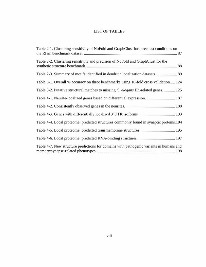
LIST OF TABLES
Table 2-1. Clustering sensitivity of NoFold and GraphClust for three test conditions on
the Rfam benchmark dataset. ............................................................................................ 87
Table 2-2. Clustering sensitivity and precision of NoFold and GraphClust for the
synthetic structure benchmark. ......................................................................................... 88
Table 2-3. Summary of motifs identified in dendritic localization datasets. .................... 89
Table 3-1. Overall % accuracy on three benchmarks using 10-fold cross validation. .... 124
Table 3-2. Putative structural matches to missing C. elegans Hh-related genes. ........... 125
Table 4-1. Neurite-localized genes based on differential expression. ............................ 187
Table 4-2. Consistently observed genes in the neurites. ................................................. 188
Table 4-3. Genes with differentially localized 3’UTR isoforms. ................................... 193
Table 4-4. Local proteome: predicted structures commonly found in synaptic proteins.194
Table 4-5. Local proteome: predicted transmembrane structures. .................................. 195
Table 4-6. Local proteome: predicted RNA-binding structures. .................................... 197
Table 4-7. New structure predictions for domains with pathogenic variants in humans and
memory/synapse-related phenotypes. ............................................................................. 198
ix
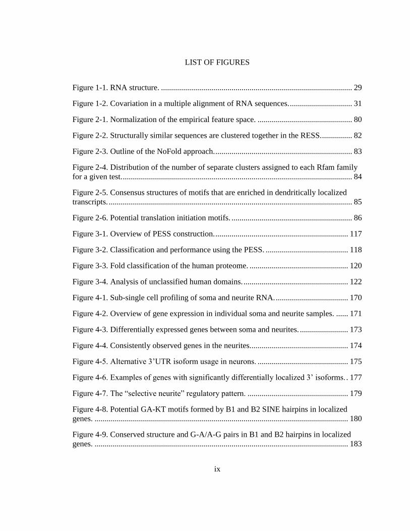
LIST OF FIGURES
Figure 1-1. RNA structure. ............................................................................................... 29
Figure 1-2. Covariation in a multiple alignment of RNA sequences. ............................... 31
Figure 2-1. Normalization of the empirical feature space. ............................................... 80
Figure 2-2. Structurally similar sequences are clustered together in the RESS. ............... 82
Figure 2-3. Outline of the NoFold approach. .................................................................... 83
Figure 2-4. Distribution of the number of separate clusters assigned to each Rfam family
for a given test. .................................................................................................................. 84
Figure 2-5. Consensus structures of motifs that are enriched in dendritically localized
transcripts. ......................................................................................................................... 85
Figure 2-6. Potential translation initiation motifs. ............................................................ 86
Figure 3-1. Overview of PESS construction. .................................................................. 117
Figure 3-2. Classification and performance using the PESS. ......................................... 118
Figure 3-3. Fold classification of the human proteome. ................................................. 120
Figure 3-4. Analysis of unclassified human domains. .................................................... 122
Figure 4-1. Sub-single cell profiling of soma and neurite RNA. .................................... 170
Figure 4-2. Overview of gene expression in individual soma and neurite samples. ...... 171
Figure 4-3. Differentially expressed genes between soma and neurites. ........................ 173
Figure 4-4. Consistently observed genes in the neurites................................................. 174
Figure 4-5. Alternative 3’UTR isoform usage in neurons. ............................................. 175
Figure 4-6. Examples of genes with significantly differentially localized 3’ isoforms. . 177
Figure 4-7. The “selective neurite” regulatory pattern. .................................................. 179
Figure 4-8. Potential GA-KT motifs formed by B1 and B2 SINE hairpins in localized
genes. .............................................................................................................................. 180
Figure 4-9. Conserved structure and G-A/A-G pairs in B1 and B2 hairpins in localized
genes. .............................................................................................................................. 183

x
Figure 4-10. Comparison of the most common structural folds represented in different
proteome sets. ................................................................................................................. 184
Figure 4-10. Protein structures of the locally-translated proteome. ................................ 185
1
Chapter 1: Introduction
As an introduction to the computational structure analysis tools and biological
applications that will be presented in the main body of this thesis, I review here the basics
of ribonucleic acid (RNA) secondary structure, protein tertiary structure, and the
fundamental concepts of synaptic plasticity and long-term potentiation in neurons,
focusing in particular on areas where structure analysis can yield new insight into
biological function.
1.1. RNA structure
RNAs are versatile macromolecules that play a wide variety of roles in the cell—
most notably as a mobile templates coding for proteins, but also sometimes as
independent regulatory or catalytic molecules [1,2]. RNAs self-base pair to form various
structures that help define their function and regulation. Below I review the basics of
RNA structure, including how it can be predicted and examples of functional structures.

2
1.1.1. Overview
RNA is a single-stranded polymer made up of a chain of individual nucleotides,
each composed of a ribose sugar with a phosphate group at the 5’ position, a nitrogenous
base at the 1’ position, and hydroxyl groups at the 2’ and 3’ positions. Nucleotides are
joined together by a phosphodiester bond between the phosphate group of one nucleotide
and the 3’ hydroxyl of another. Thus the final RNA polymer has directionality, where one
end has a free phosphate group (called the 5’ end) and the other end has a free hydroxyl
(called the 3’ end). The 5’ end is considered the “beginning” of the molecule, since
translation (the synthesis of protein from RNA) proceeds in a 5’ to 3’ direction.
There are four canonical types of bases used in RNA: adenine (A), guanine (G),
cytosine (C), and uracil (U). Certain bases can form hydrogen bonds with each other to
create base pairs. The standard “Watson-Crick” base pairs are G-C and A-U, but other
pairings, most notably G-U “wobble” pairs [3], are also possible under certain conditions.
Base pairing is energetically favorable, and therefore the single strand of a given RNA
will tend to form base-pairing interactions with itself when possible. This causes each
RNA to take on a shape determined by the base pairs that occur. The two-dimensional
conformation of an RNA that results from base pairing is generally referred to as its
“secondary structure”, whereas the linear sequence of nucleotides that make up the RNA
is called its “primary structure”.
RNA secondary structures can be broken down into a relatively small set of
building blocks. One of the most common building blocks is the stem-loop (or “hairpin”)
structure. Stem-loops consist of a “stem” of consecutive paired bases, and a “loop” of at

3
least three unpaired bases, where the single strand of RNA loops back around to pair with
itself at the stem (Fig. 1-1A). Stem-loops are often interrupted by interior loops, which
are regions of one or more unpaired bases within the stem; or by bulges, which are
interior loops where only one side of the stem is unpaired. Branches may also occur
where two or more stems split from a single stem, sometimes accompanied by internal
loop (Fig. 1-1A).
The definition of secondary structure is generally restricted to only base pairing
interactions that result in well-nested structures (i.e. interactions that do not cross over
each other) (Fig. 1-1B). However, RNA structure also has an important three-dimensional
component, referred to as its tertiary structure. For example, stem-type secondary
structures form a helix in three-dimensional space (Fig. 1-1C), and this helix can have
different properties and shapes depending on the combination of base pairs that form the
stem and the presence of bulges or interior loops [4]. Non-nested base pairing interactions
are also possible, including pseudoknots, which are regions of base pairing interactions
that cross over each other (Fig. 1-1D), and G-quadruplexes, which are formed by
interactions between repeated groups of guanines to form a four-stranded structure (Fig.
1-1E) [4].
1.1.2. RNA structure prediction
Experimental methods

4
Until recently, experimental methods for probing RNA secondary structure were
relatively low-throughput. Classic methods include X-ray crystallography, nuclear
magnetic resonance (NMR) spectroscopy, single-strand RNA (ssRNA)- or double strand
RNA (dsRNA)-specific chemical modification followed by primer extension (e.g.
SHAPE [5]), and ssRNA/dsRNA nuclease cleavage followed by fragment size analysis
[6]. These methods, though accurate, are time consuming and difficult to apply to
multiple RNAs in parallel. New methods for structure probing combine various chemical-
and nuclease-based techniques with high-throughput RNA sequencing to greatly increase
the number of RNAs that can be probed at once [7]. Although these methods show great
promise, they do not always give complete information for all RNAs, and have not yet
been applied to all species. Because of this, computational structure prediction methods
continue to be developed to fill the holes in existing RNA structure data.
Computational methods
Given a set of parameter values defining the change in free energy associated with
different base pairs (i.e. their stability), and assuming that all secondary structures will be
well-nested, then the “optimal” secondary structure—that is, the structure with the
minimum free energy (MFE)—for any given RNA sequence can be found in using a
dynamic programming algorithm [8–12]. These thermodynamic modeling-based
approaches are still widely used today to predict secondary structure in the absence of
other sources of information. Although these methods are relatively fast, their main
drawback is that the MFE structure is often not the structure taken on in vivo, due to
5
external factors such as protein binding to the RNA or changes in environmental ion
concentration [1]. The differences between the MFE structure and true in vivo structure
are particularly apparent for longer (>700nt) sequences, for which only about 60% of
predicted base pairs are estimated to be correct on average [1].
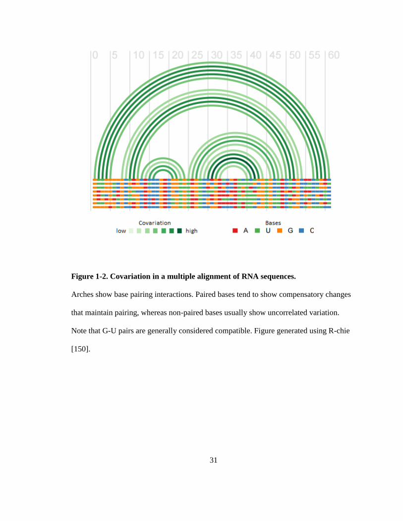
One way to improve the accuracy of in silico secondary structure prediction is to
use comparative information across multiple homologous RNAs. If the structure of the
RNA is functionally important, it may show a pattern of conservation called
“covariation”. Covariation is when there are compensatory base changes that maintain
base-pairing potential of the sequence. In a multiple sequence alignment of homologous
RNAs, this manifests as columns of the alignment with pairing-compatible changes—for
example, when the base in one column changes from a G to an A, the base in the other
column changes from C to U (Fig. 1-2). Such a change maintains the ability of the RNA
to form a base pair between those particular bases. The observation of multiple
compensatory changes across evolution provides strong evidence for in vivo base-pairing
interactions, and can therefore be used to guide structure prediction [13–17]. Often, this is
used in combination with thermodynamic modeling to arrive at the final structure
prediction [18–21]. Although these covariation-based methods can be very accurate, they
are much more computationally intensive than thermodynamic modeling alone due to the
need to calculate a multiple alignment of the input sequences. This method is therefore
not feasible for all applications, as will be discussed further in Chapter 2.

6
1.1.3. Structure-function relationships
One of the primary roles of RNA is to serve as a template for the creation of
proteins. Within protein-coding RNAs, also known as messenger RNAs (mRNAs), three
functionally distinct regions are defined: the coding region (CDS), which is the part of
the mRNA that is translated into protein; the 5’ untranslated region (UTR), which is
upstream of the CDS and is not translated; and the 3’UTR, which is downstream of the
CDS and also not translated. The 5’UTR is generally relatively short (a few hundred
nucleotides (nt)), but can occasionally contain sequence and structure motifs that help
recruit and position translational machinery, such as the ribosome, at the correct start site
of the CDS [22–24]. The 3’UTR, on the other hand, is often much longer (up to several
thousand nt) and contains a rich variety of sequence and structure motifs involved in
various aspects of mRNA regulation, including subcellular localization, translation, and
degradation [25].
There are several mechanisms by which secondary structures can play a functional
role in the mRNA. Most prominently, structures often serve as binding sites for RNA-
binding proteins (RBPs). Depending on the RBP, it may be the RNA structure itself that
is recognized (e.g. binding of the RBP Staufen to dsRNA [26]), or the structure may help
position a linear sequence of unpaired nucleotides (e.g. within a loop) into a more
favorable position for recognition [27]. Once bound, RBPs can initiate and regulate a
variety of different functions. For example, Staufen2 likely helps mediate dendritic
localization of the RNAs to which it binds [28,29]. Another example is the ADAR
(adenosine deaminase acting on RNA) RBPs, which bind to long stems of dsRNA and

7
perform RNA editing to change adenines to inosines [30]. Conversely, a secondary
structure can also function by occluding a binding site for an RBP or microRNA,
blocking those molecules from binding. In rare cases, secondary structures mediate
function by mimicking or replacing other molecules. For example, an mRNA from the
cricket paralysis virus contains an internal ribosome entry site (IRES) that mimics the
structure of tRNA-Met and forms a pseudoknot with the initiation codon. This allows the
virus to initiate translation in the absence of canonical initiation factors [31,32].
Another large class of RNA is non-coding RNA (ncRNA), which includes
functionally diverse subclasses such as microRNAs (miRNAs), transfer RNAs (tRNAs),
ribosomal RNAs (rRNAs), long non-coding RNAs (lncRNAs), among others [33]. For
these RNAs, structure is often a vital determinant of function [34]. For example, the
cloverleaf structure of tRNA is strongly conserved across species, despite substantial
variation on the sequence level (46% pairwise identity on average according to the Rfam
database [35]), which allows it to associate with the ribosome. In the case of ribozymes,
such as 23S rRNA, RNaseP, and self-splicing introns, the structure of the RNA actually
confers independent catalytic activity to the RNA [33]. For other ncRNAs, structure plays
the most important role during biogenesis. Examples of this are the hairpin structures of
pri- and pre-miRNA that are necessary for cleavage into mature miRNA by Drosha and
Dicer proteins [36]. There are many more examples of functional ncRNA structures in
the literature, and many families of such structures have been compiled into the Rfam
database [35].

8
There are two particular ideas worth noting regarding the structure-function
relationship of RNA. The first is that if we know of a structure that plays a functional role
in one RNA, we can search the transcriptome for similar structures to identify other
RNAs that have a common function (in the case of ncRNAs) or are co-regulated by the
same RBP or pathway (in the case of mRNA regulatory motifs). This is the basis of the
Rfam database [35], which uses covariance models—a type of stochastic context-free
grammar that can model both sequence and secondary structure—to scan for new
instances of known functional structures. Secondly, and relatedly, if we know a set of
mRNAs are co-regulated, we can look for structural motifs shared between them to find
candidates for the regulatory element or RBP binding site. Computational methods for
performing this particular kind of analysis are currently lacking due to the difficulty of
obtaining accurate structure predictions for large datasets and the difficulty of measuring
the notion of similar secondary structures. This problem will be addressed in Chapter 2.
1.2. Protein structure
Proteins are the main workhorses of the cell, participating in almost all aspects of
cellular function, including gene expression, energy production, signaling, catalysis,
transport, and cytoskeleton formation. Structure is an indispensable aspect of function for
almost all proteins, and even small disruptions of structure can lead to serious diseases
[37]. In this section, I review the basics of protein structure-function relationships and
how they can be predicted.

9
1.2.1. Overview
A protein is composed of a linear chain of amino acid residues linked by peptide
bonds between the carboxyl group of one amino acid and the amino group of the next.
There are 20 canonical amino acids that vary in size, charge, hydrophobicity, polarity,
and modifiability. The unique combination and ordering of residues in a protein are the
basis for protein structure and function.
Protein structure is often described as having four levels: primary, secondary,
tertiary, and quaternary. The primary structure is simply the linear sequence of amino
acids making up the protein. The secondary structure is defined as the local patterns of
hydrogen bonding between a carboxyl oxygen and amino hydrogen of nearby residues.
The most common and stable secondary structures are the α-helix [38] and β-sheet [39],
but other conformations such as coils and turns are also observed. Tertiary structure is the
full three-dimensional conformation of the protein, which is stabilized by covalent
interactions, hydrogen bonds, hydrophobic interactions, van de Waals forces, electrostatic
interactions, and repulsive forces. It is the tertiary structure that is considered most
important for overall function of most proteins, although individual primary and
secondary features can also have functional roles. Finally, the quaternary structure refers
to the organization of multiple separate protein chains into a functional complex.
Many proteins have smaller subregions called domains. In the context of structural
biology, a domain is usually defined as a compact, stable, independent folding unit
[40]—that is, if the domain sequence were to be cleaved from the rest of the protein, it
would still take on its native, stable tertiary structure. Alternatively, in the context of
10
evolutionary sequence analysis, a domain is defined as a conserved region of the protein
sequence, often with a conserved function (for example, the domains defined in the Pfam
database [41] are of this type). It is important to note that in practice these two definitions
often coincide, since structural domains are usually evolutionarily conserved and have a
specific function [40]. The definition of a structural domain is broader, however, because
it is possible for non-homologous sequences to have the same structure. In this thesis, I
will primarily use the word “domain” to refer to the union of these definitions, and
specify “structural domain” or “sequence domain” when distinction is necessary.
A remarkable feature of domains is their modularity. Most proteomes appear to be
composed of a finite library of domains that have been “mixed and matched” to produce
various functional combinations within multi-domain proteins [40]. Due to accumulated
sequence variation over time, the instances of a domain have varying levels of sequence
similarity across different proteins and species. Many domains have become so diverged
that it is impossible to recognize them based on sequence alone. In these cases, structural
information can be used to identify domains, because structure is usually more conserved
than sequence [42]. Given the complexity of relationships between domains, several
hierarchical classification schemes have been created to organize domain instances (that
is, individual observations of a domain in a protein) based on defined levels of similarity
and evolutionary relationship. The Structural Classification of Proteins (SCOP) database,
for example, manually curates groups of domains on four main levels: family,
superfamily, fold, and class [43]. “Families” group together homologous domains with
highly similar sequence and closely related function (although there can be fine-grained
11
functional differences between members of a family, such as different binding
preferences for DNA-binding domains). “Superfamilies” group together families with
more divergent, but still recognizable, sequence similarities. Superfamilies also tend to
have a general conserved function. The next level is “fold”, which groups together
superfamilies with similar tertiary structures (that is, similar numbers and topological
arrangements of secondary structures). Folds are defined purely based on structure, and it
is not always clear if the constituent superfamilies are related evolutionarily or have
arrived at similar structures by convergent evolution. Nonetheless, members of a fold
typically still have similar coarse-grain functions, with the exception of some highly
diversified and prevalent “superfolds”, which have been adapted to a variety of distinct
purposes [44]. Interestingly, there appears to be a limited number of folds used by natural
proteins—only a little over 1,000 folds are currently defined, and the rate of new fold
discoveries has steadily declined over the past few years. Finally, the “class” level of
SCOP groups folds very roughly based on overall secondary structure composition and
other properties, such as all-α-helix, all-β-sheet, mixed-α-β, membrane proteins, and a
few others. Overall, this taxonomically-inspired classification scheme (and others, such
as CATH [45]) provides a convenient discretization of domain similarity that enables
analysis at defined levels of evolutionary and structural relationship.
1.2.2. Protein structure prediction
Experimental methods
12
Protein tertiary structure can be experimentally determined (“solved”) using
several methods, most commonly X-ray crystallography and NMR spectroscopy. X-ray
crystallography requires purification and crystallization of the protein of interest, which is
then exposed to X-rays to obtain a diffraction pattern. This diffraction pattern is analyzed
to infer the location of atoms in the structure. Although crystallography can be very
accurate, it is limited by the difficulty of obtaining protein crystals. Proteins with flexible
domains are particularly difficult to crystalize, and must be split into non-flexible
fragments to obtain partial crystal structures. NMR spectroscopy, on the other hand, is
well-suited for flexible proteins, since it works on proteins in solution and does not
require crystallization. NMR spectroscopy measures atomic resonance while exposing the
protein to various radio frequencies in a strong magnetic field, which can be analyzed to
identify nearby atoms in the structure. This is then used to infer the three-dimensional
structure. The drawbacks of NMR spectroscopy are that it is generally limited to only
small proteins, cannot be used for insoluble proteins such as membrane proteins, and has
low spatial resolution. Recently, another method called Cryo-electron microscopy (Cryo-
EM) has improved in resolution to the point where it can be used for atomic-level
structure solving. Cryo-EM has promise to alleviate several of the difficulties facing
crystallography, since it freezes molecules rather than crystalizing them, but the method
is still under development [46]. Overall, all three methods are limited to various degrees
by expense and throughput capacity, and because of this only a fraction of known protein
sequences have been structurally characterized. This has motivated the development of a
wide array of computational structure prediction methods.
13
Computational methods
Computational methods for predicting protein tertiary structure can generally be
divided into two categories: ab initio and template-based [47]. Ab initio (or de novo)
methods attempt to determine a protein’s structure directly from the sequence using first-
principles molecular dynamics simulations. However, due to the enormous search space
of possible three-dimensional conformations for an average-sized protein, ab initio
methods are generally only computationally feasible for the smallest proteins [48].
Therefore, template-based modeling has been the more popular method over the last two
decades.
Template-based modeling covers a wide variety of methods that make use of
currently known information about protein structures—e.g. experimentally solved protein
structures in the Protein Data Bank (PDB) [49]—as a starting point (or “template”) for
predicting the structures of new proteins. Template-based modeling can be subdivided
into two main types: homology modeling and threading. Homology modeling, also called
comparative modeling, uses sequence alignment methods to match a query sequence to
any homologous sequences within the database of structurally-solved proteins. These
methods work on the assumption that homologous proteins are likely to share a
conserved structure, and therefore the structure of the homolog can be used to predict the
structure of the query. Homology modeling methods such as HHPred [50]—which uses
hidden Markov model (HMM)-based profile-profile alignments to increase sensitivity—
have demonstrated good results when a homolog can be detected. However, the major

14
challenge facing these methods is the difficulty of detecting more remote homologs—
those falling within the “twilight zone” of sequence similarity, usually <30% identity
[51]. This includes a large fraction of proteins at the current time, and has thus motivated
the second template-based method—threading. Threading or “fold recognition” methods
do not require homology or sequence similarity with a structurally solved protein in order
to work, but instead try to directly use structural information to find the best match for
the query. Briefly, threading comprises aligning a query sequence to a structural
“template”, defined in this context as the three-dimensional coordinates of atoms derived
from a known protein structure (usually with the side chains removed). The best
alignment between the query and structure is determined based on the compatibility of
residue contacts, secondary structures, solvent access, and other criteria. This process is
then repeated for every template in the database to identify which structure gives the most
thermodynamically favorable structure for that sequence. Although threading has the
advantage of working even in the absence of homology between the query and template,
it is limited by much greater computational costs than homology modeling. Nonetheless,
threading is much more tractable than ab initio methods, and thus has been used
extensively and to good success over the last several years [51].
More recently, a third category of methods has emerged that combines aspects of ab
initio and template-based methods [47]. These hybrid methods usually cut the protein
sequence into many smaller fragments, and then attempt to match each fragment to one
or more templates (which themselves are fragments of known structures). Once template
candidates have been identified, ab initio methods are used to assemble the fragments

15
into a conformation that is energetically favorable for the protein as a whole. Using the
templates as a starting point greatly limits the search space, making the ab initio
simulations more tractable. I-TASSER [52] and Rosetta [53] are two examples of highly
successful hybrid methods. However, these methods are still too slow to be applied to
large scale projects, such as whole-proteome structure prediction.
1.2.3. Structure-function relationships
There is a strong association between structure and function among proteins.
Proteins with similar structure very often have similar function [54], and—to a lesser
extent—proteins with similar function may have similar structure. This has been shown
to hold true even for highly disparate amino acid sequences, and is the main motivation
behind the field of structural genomics, which makes extensive use of the experimental
and computation methods described above to make inferences about function based on
structural similarities between proteins on a genome scale [55].
There are limits to the amount of functional information that can be gained simply by
matching proteins to similar tertiary structures. For one thing, since structure prediction is
usually done on the level of individual domains, this information must be integrated to
understand the overall function of multi-domain proteins. Secondly, many of the nuances
of domain function are influenced by fine-grained differences in the arrangement of
secondary structures or by variation of specific residues in a binding pocket or enzymatic
active site. This is particularly evident in the case of “superfolds”; for example, the TIM
barrel fold is primarily found in enzymes, but consists of at least 60 distinct enzyme
16
commission (EC) classes [44]. Finally, a large fraction of proteins include “intrinsically
disordered” regions that do not take on a well-defined native tertiary structure. These
regions often serve as flexible linkers between domains in multi-domain proteins, or may
only fold when bound by a cofactor [47,56]. The function of these regions is therefore not
amenable to typical structure-based analysis.
Despite these limitations, structure prediction has proved to be an extremely useful
first step towards a functional understanding of uncharacterized proteins [54]. Improving
the speed of methods for recognizing structural similarities, especially in the absence of
sequence similarity, will greatly increase our capability for genome-scale annotation of
protein function. A new approach to this problem will be discussed in Chapter 3.
1.3. Neurons, plasticity, and structure
Neurons are highly polarized cells consisting of a cell body (soma), and long,
branched processes (usually a single axon and multiple dendrites). The flow of
information through the neuron typically proceeds from the dendrites, which receive
signals from other neurons at synapses; to the soma, which integrates signals; and finally
to the axon, which transmits signals to other neurons. Synapses show a remarkable ability
to remodel themselves in response to stimulation, becoming more or less responsive to
future inputs (synaptic plasticity). This is thought to be one of the mechanisms underlying
the larger scale phenomena of learning and memory in the brain. Here, I will survey
important concepts related to synaptic plasticity in pyramidal neurons of the CA1
17
hippocampus, which have been studied extensively in this context, and highlight areas
where structure analysis can help further our understanding.
1.3.1. Components of pyramidal neurons
Pyramidal neurons exist in a wide variety of mammals and are generally found in
brain structures associated with complex cognitive function [57,58]. The morphology of
pyramidal neurons is characterized by a single axon with many branches that make
excitatory glutamatergic synapses with other neurons, as well as an extensive dendritic
arbor with mostly excitatory synaptic inputs [58]. Pyramidal neurons may also receive
some synaptic inputs on the axon and soma, which are typically inhibitory GABAergic
synapses [58].
An important set of substructures of pyramidal dendrites are the dendritic
spines—small, knob-like protrusions along the dendrites which are the site of most
glutamatergic synapses. Spines vary widely in size and shape [59] and show
morphological and functional plasticity over time [60–62]. A single pyramidal neuron
may have thousands of dendritic spines, occurring at a density of about 1-10 spines per
µm of dendritic length in mature neurons [59]. Although the precise purpose of spines is
unclear, one of their main functions is likely to compartmentalize synapses and help
prevent important molecules from diffusing away [63,64]. The spine neck may also serve
to modulate electrical conductance properties [65]. Abnormal spine morphology has been
observed in many neurological disorders, including Down Syndrome [66], Fragile X
Syndrome [67], and epilepsy [68].

18
Dendrites also contain a variety of organelles, including abundant mitochondria
[69], endoplasmic reticulum (ER) [70–73], Golgi “outposts” [70], and multivesicular
bodies [71,73]. An organelle called the “spine apparatus” has also been observed in
dendrites [74,75], which appears in 10-15% of mature hippocampal spines [71]; however,
the exact function of this organelle is not currently well understood. In addition to
organelles, many components of the translational machinery have been found in dendrites
at the base of spines, including tRNAs, polyribosomes, and initiation/elongation factors
[76–78].
1.3.2. Long-term potentiation
The idea that the plasticity of synapses could play a central role in learning and
memory was suggested over a century ago by Santiago Ramόn y Cajal [79]. In 1949,
Donald Hebb formalized a model of how synaptic plasticity relates to learning and
memory [80], but it was not until about 20 years later that substantial evidence for a
molecular basis of such a model was provided by the discovery of long-term potentiation
(LTP) [81,82]. These studies showed that stimulating excitatory hippocampal synapses
resulted in a long-lasting increase in synaptic strength of those synapses. Since then, LTP
has become an area of intense research in the field of neuroscience, and remains one of
the leading hypotheses of the molecular basis of learning and memory [83,84]. Although
there are now thought to be multiple forms of LTP, which depend on factors such as
brain region and stimulation frequency [84], I will focus here on N-methyl-D-aspartate
(NMDA) receptor-dependent LTP that occurs in the CA1 region of the hippocampus.
19
LTP is often described as having two stages: an early phase (E-LTP), usually
defined as the first 1-3 hours after stimulation; and a late phase (L-LTP), which requires
protein synthesis and gene transcription [85]. E-LTP is triggered by activation of post-
synaptic NMDA receptors (NMDARs), which open to allow calcium influx [84]. This
activates Ca2+
/calmodulin-dependent protein kinase (CaMKII) [86], which causes a rapid
increase in α-Amino-3-hydroxy-5-methyl-4-isoxazoleprpionic acid receptors (AMPARs)
in the synapse membrane [87]. The exact mechanism by which CaMKII influences
AMPAR synaptic trafficking is currently unclear. Several early studies suggested that
CaMKII phosphorylates the carboxy-terminal tail (C-tail) of AMPAR subunit GluA1
and/or AMPAR-accessory proteins [84]. In contrast, a recent set of studies has suggested
that the C-tail of GluA1 is not needed for normal LTP, and furthermore, AMPARs can be
completely replaced with kainite receptors without a substantial impact on LTP [84,88].
There is also conflicting evidence about which other signaling cascades, besides that
mediated by CaMKII, might be important for LTP. Many molecules have been
discovered that seem to modulate LTP, but few besides CaMKII have been shown to be
vital [83]. These results show that despite substantial progress over the past 20 years,
there is still much that is not well understood about this process.
The second phase, L-LTP, is dependent on new protein translation. Furthermore,
this new translation often occurs in the dendrites themselves, in close proximity to the
activated synapse [89]. There is now substantial evidence that a subset of neuronal
mRNAs are actively localized to the dendrites, usually in a translationally repressed state,
and then translated locally in or near spines in response to synaptic activation. The topics

20
of mRNA localization and local translation are discussed in more detail in the next two
sections. It is worth noting that there is also evidence for an important role of new
transcription for L-LTP [90], which will not be reviewed extensively here.
Beyond changing the molecular composition of the synapse, LTP also causes (and
possibly is perpetuated by) changes in the shape and size of the spine in which the
synapse is housed [69]. The mechanisms of how this occurs are still being investigated,
but filamentous actin (F-actin) polymerization dynamics likely play an important role
[69,84]. F-actin makes up one of the major structural components of spines, and
inhibition of actin polymerization prevents spine growth and LTP [91,92]. Activity-
dependent cytoskeletal growth may be due to CaMKII activation of Rho GTPases, which
promote actin polymerization, although how this occurs is not known [84]. It is
hypothesized that these changes in structure may help promote AMPAR incorporation
into the synapse, and thus promotes LTP [84]. After increasing in size, the spine can be
further stabilized by cell adhesion molecules, such as N-cadherin, which has been shown
to increase after synaptic activity [69].
1.3.3. Importance of RNA localization and local translation
Direct evidence for the idea that new protein synthesis was required for memory
formation was first demonstrated in the 1960s, where it was shown that mice injected
with the protein synthesis inhibitor puromycin to the temporal lobe showed impaired
long-term memory formation if the injection was given within three days [93]. A large
number of follow-up studies corroborated the potential importance of new protein
21
synthesis in a variety of memory-related behaviors [94]. On the molecular level,
treatment with the protein synthesis inhibitor anisomycin was shown to inhibit spine
enlargement during LTP [95], lending further support that LTP might form the molecular
basis of learning and memory. However, these studies at first did not directly address the
question of where within the neuron this new protein synthesis was occurring, and it was
generally assumed that it would occur in the soma [85].
Following the discovery of polyribosomes [76] and multiple mRNAs [96–98] in the
dendrites, the idea that translation could occur locally in the dendrites began to gain
popularity. This model was attractive for several reasons. For one, it provided a simple
mechanism by which newly synthesized proteins could be sorted to the correct synapse:
synaptic activation could trigger translation of only those mRNAs in the vicinity of the
spine, thus causing a local increase in new proteins at the activated synapse. Other
theoretical benefits include reduced transport costs, faster response time, and prevention
of toxic ectopic protein expression [99,100]. Finally, in 1996, two studies provided direct
evidence that protein synthesis can in fact occur locally in isolated dendrites [101] and
hippocampal tissue slices [102].
Although local translation is now generally accepted as being important for lasting
synaptic potentiation [103], there is less known about exactly which mRNAs are
localized and what roles individual locally-translated proteins play in LTP. As techniques
for profiling and quantifying RNA have improved, estimates of the dendritic
transcriptome have expanded from a few RNAs [98] to a few hundred [104–107] to
possibly even a few thousand [108,109]. There are several RNAs that are considered

22
“gold standard” localized RNAs, which have been observed by multiple labs and
methods to be robustly localized to the dendrites, such as CaMKIIα, β-actin, Arc, and
BC1. But overall, there has been surprisingly little concordance between different
analyses of the dendritic transcriptome, even when the same organism and brain region
are profiled. In terms of understanding the actual functional role of individual localized
mRNAs and their protein products, even more work remains to be done. To show
specifically that local translation of a particular protein is important for LTP, an ideal
experiment would disrupt only the local translation of that protein without altering its
somatic expression. So far, this has mostly been accomplished in a few isolated cases,
usually by abolishing the dendritic localization of the mRNA. For example, in mice
lacking the 3’UTR of CaMKIIα mRNA, which contains its dendritic targeting sequence,
it was shown that protein levels of CaMKII at the synapse were greatly reduced and L-
LTP was impaired [110]. Much more work remains to be done to understand the role of
the many potential locally-translated proteins in LTP.
1.3.4. Mechanisms of dendritic RNA localization: a role for structures
Proper localization of RNAs to the dendrites is a prerequisite for local translation,
and therefore for long-lasting synaptic potentiation. Dendritic localization is thought to be
mediated by specific RNA-binding proteins (RBPs) that recognize sequence or structure
motifs on their target RNAs [100,111,112]. These RBPs may recruit other proteins to the
RNA, forming a ribonucleoprotein complex (RNP). The RNP typically includes proteins
that interact with motor proteins such as kinesin and dynein [113–115], which move

23
along microtubules in the soma and dendrites to bring the RNP to its destination. While
in the dendrites, RNA is mostly kept in a translationally repressed state by proteins in the
RNP [115–117]. This repression is then relieved when a nearby synapse is activated,
allowing for local production of proteins [117,118].
Interactions between RBPs and RNAs are vital for proper localization, and much
work has been done to try to identify the dendritic targeting elements (DTEs) on localized
RNAs that are recognized by RBPs. Identifying these DTEs would have benefits such as
(1) allowing us to predict additional localized RNAs based on the presence of similar
motifs, (2) enabling the identification of co-regulated groups of RNAs based on the
presence of shared DTEs, and (3) providing insights into how dysregulation of RBP
binding and RNA localization can lead to disease. Thus far, however, the identification of
DTEs has been challenging. Below I briefly outline what is known about the localization
and DTEs of a few of the most well-characterized dendritic RNAs and localization-
mediating RBPs.
BC1 RNA. Brain cytoplasmic RNA 1 (BC1) is a short (~150nt), structured non-
coding RNA that is dendritically localized [119] and plays a potential role in translational
regulation [120]. The stem loop structure at its 5’ end has been experimentally
determined [121] and is likely the DTE [122]. A particular part of the stem loop forms a
GA kink-turn motif and seems to be bound by hnRNP-A2, which mediates the
localization [123]. A type of short interspersed nuclear element (SINE) called the ID
element is derived from BC1 [124] and has also been shown to act as a DTE in several
dendritic RNAs in rat [125,126].
24
Staufen. The Staufen family of proteins (Stau1 and Stau2) are RBPs that bind
dsRNA such as that found in stem-loop structures. Stau1 is ubiquitously expressed across
tissues and may play a role in L-LTP [127]. Stau2 protein is enriched in the brain [100],
shuttles to the dendrites in RNPs [128], and is likely involved in dendritic localization
[28]. Several secondary structures have been proposed to be bound by Stau2 [129], which
appear mostly sequence-independent.
ZBP1 and β-actin. A 54nt region in the 3’UTR of β-actin, known as the “zipcode”
sequence, is necessary and sufficient for its localization in several cell types [130].
Binding of zipcode-binding protein 1 (ZBP1, called IMP-1 in human) to the zipcode was
found to be important for both the localization and translational inhibition of β-actin
[131,132]. Later studies showed that most of the zipcode actually functions as a spacer
for two much shorter motifs that are bound by two KH domains of ZBP1, and that similar
bipartite motifs were conserved in other mouse/human mRNAs, making them potential
targets of ZBP1 as well [133].
FMRP. Fragile-X mental retardation protein (FMRP) is thought to play an
important role in translational repression of localized mRNAs and possibly also
modulates localization [116]. It appears to bind to a wide variety of localized RNAs,
including CaMKIIα, Map1b, PSD-95, and Fmr1 (its own mRNA) [100]. It has been
proposed to bind to G-quadruplexes through its RGG-box domain [134,135], although a
more recent study of FMRP binding using HITS-CLIP showed no enrichment for G-
quadruplexes or any other motif [136].
25
hnRNP-A2. Heterogeneous ribonucleoprotein particle A2 (hnRNP-A2) binds to
known dendritically localized RNAs such as CaMKIIα and Arc [137] and is thought to be
directly involved in localization. Multiple motifs have been proposed to be recognized by
this RBP, including a pair of 11nt sequences (the hnRNP-A2 recognition element, A2RE)
first identified in the MBP mRNA in oligodendrocytes [138], G-quadruplex structures
and CGG repeats [139,140], and GA kink-turn structural motifs [123].
CaMKIIα. Although it is one of the most extensively studied dendritically localized
mRNAs, CaMKIIα still does not have a fully defined DTE. Most reports point to an
element in the 3’UTR, but there is conflicting evidence about the minimal element
needed for localization [110,123,141–143]. Implicated regions so far include both linear
sequences and secondary structures.
A common theme in many of these examples is the lack of consensus regarding the
location and nature (linear or structural) of DTEs on specific transcripts. Part of the
problem may be that some localized RNAs in fact have multiple DTEs, each regulating
distinct and/or redundant aspects of the localization process [99]. An interesting example
of this is BC1, which was shown to have two sub-motifs within its DTE: one that was
needed for nuclear export and another that was needed for transport to the distal dendrites
[123]. Adding to this difficulty, many DTEs are now known to have a secondary structure
component that is either central to or supports recognition by the RBP [144], which may
have contributed to conflicting reports in the past that mostly focused on linear sequence
DTEs. Given that there are hundreds or even thousands of localized RNAs in neurons, it
seems unlikely that each one has a unique DTE and RBP mediating its localization. A
26
more likely explanation is that multiple localized RNAs share DTEs and are recognized
by the same RBP, but we are missing these signals due to a lack of tools that perform de
novo RNA structure motif discovery in large datasets.
1.3.5. Protein structures of the synapse
One of the gaps in our understanding of long-lasting synaptic potentiation is the
specific role of each locally-translated protein in this process. Although experimental
work will be needed to pick apart exact functions, we can make some initial guesses
using computational annotation methods. Structure-based functional annotation may be
of particular use in this case, given that there are a variety of important roles for protein
structures at the synapse. Examples include the PDZ domain in scaffold-associated
proteins [145]; cadherins, neurexins/neuroligins, ephBs/ephrin-B, and immunoglobulin-
containing cell adhesion folds at the synaptic junction [146]; transmembrane folds in
membrane-bound channels and receptors; kinase and phosphatase catalytic folds involved
in signaling and synaptic plasticity; and many others. Although many of the proteins
containing these structures are likely to be constitutively present at the spine or post-
synaptic density (surveyed in [147–149]), and thus may be primarily synthesized in the
soma, it would be interesting to see if a subpopulation of these proteins is locally
translated as well, and if new examples of these folds can be discovered. Furthermore,
recent genome-wide analyses of neurological diseases have revealed enrichment for
causative mutations in synaptic proteins in human and mouse [147,149], several of which
have been shown to disrupt important structural binding sites. A better understanding of
27
the structures of locally translated proteins will help guide future experimental work and
aid in predicting the functional impact of mutations.
1.4. Overview of thesis
In this thesis, I present two new methods for structure-based analysis of large-
scale datasets based on the concept of empirical feature spaces—feature spaces defined
by examples of natural structures—and then apply these methods to address the questions
outlined above regarding the localization of RNA in the dendrites of neurons and the
possible roles of locally translated proteins.
In Chapter 2, I describe the RNA empirical structure space (RESS), which uses
Rfam covariance models to map uncharacterized RNAs to a structural feature space. I
will show that RNAs with similar structure cluster together within the RESS, even in the
absence of sequence similarity, and use this fact to develop a pipeline for de novo
secondary structure motif discovery that can be applied to finding functional motifs
enriched in co-regulated transcripts. Since this method scales linearly with increasing
input dataset size, it is feasible to run on thousands of sequences at once.
In Chapter 3, I describe the protein empirical structure space (PESS), which uses
threading against a small set of known structure templates to map uncharacterized protein
domain sequences to structural feature space. As with the RESS, the PESS clusters
protein sequences based on structure even in the absence of detectable sequence
similarity. I show that the PESS can be used for a variety of purposes including
classification of sequences into known folds, identification of novel folds, and finding of
28
distant homologs (or structural analogs) across species. This method saves substantial
amounts of time compared to traditional threading methods by using only a small library
of templates for threading, yet has accuracy on par with threading against a much larger
set.
In Chapter 4, I will combine experimental and computational methods, including
the two methods described above, to catalog the set of RNAs localized to the dendrites in
mouse hippocampal neurons, identify potential linear and structural localization signals,
and predict the functions of locally translated proteins based on domain-level structural
prediction. The results include findings that would be difficult to identify using
traditional sequence-based tools, demonstrating the utility of including structure-based
tools when performing functional analysis of RNA and protein.
Finally, in Chapter 5, I discuss some of the implications and future directions
suggested by this work, including several avenues where structure analysis may yield
particular insight.

29
Figure 1-1. RNA structure.
(A) An example of RNA secondary structure, showing typical motifs. (B) A well nested
structure (top) and non-nested structure (bottom). The black horizontal lines indicate an
RNA sequence and the arches show base pairing. Red and orange arches highlight the
non-nested part of the structure that crosses over itself. The top panel corresponds to the

30
structure in (A). (C) An example of RNA tertiary structure. (Image from the public
domain.) (D) An example of a pseudoknot structure, which consists of non-nested base
pairing interactions. (E) An example of a G-quadruplex structure consisting of four
repeating units of three G’s, separated by small loops.
31
Figure 1-2. Covariation in a multiple alignment of RNA sequences.
Arches show base pairing interactions. Paired bases tend to show compensatory changes
that maintain pairing, whereas non-paired bases usually show uncorrelated variation.
Note that G-U pairs are generally considered compatible. Figure generated using R-chie
[150].

32
1.5. References
1 Wan, Y. et al. (2011) Understanding the transcriptome through RNA structure.
Nat. Rev. Genet. 12, 641–655
2 Geisler, S. and Coller, J. (2013) RNA in unexpected places: long non-coding RNA
functions in diverse cellular contexts. Nat. Rev. Mol. Cell Biol. 14, 699–712
3 Varani, G. and McClain, W.H. (2000) The G-U wobble base pair. EMBO Rep. 1,
18–23
4 Butcher, S.E. and Pyle, A.M. (2011) The Molecular Interactions That Stabilize
RNA Tertiary Structure: RNA Motifs, Patterns, and Networks. Acc. Chem. Res.
44, 1302–1311
5 Wilkinson, K.A. et al. (2006) Selective 2′-hydroxyl acylation analyzed by primer
extension (SHAPE): quantitative RNA structure analysis at single nucleotide
resolution. Nat. Protoc. 1, 1610–1616
6 Kubota, M. et al. (2015) Progress and challenges for chemical probing of RNA
structure inside living cells. Nat. Chem. Biol. 11, 933–941
7 Lu, Z. and Chang, H.Y. (2016) Decoding the RNA structurome. Curr. Opin.
Struct. Biol. 36, 142–148
8 Zuker, M. and Stiegler, P. (1981) Optimal computer folding of large RNA
sequences using thermodynamics and auxiliary information. Nucleic Acids Res. 9,
133–148
9 Zuker, M. (1989) On finding all suboptimal foldings of an RNA molecule. Science
244, 48–52
10 Zuker, M. (2003) Mfold web server for nucleic acid folding and hybridization
prediction. Nucleic Acids Res. 31, 3406–3415
11 Hofacker, I.L. (2003) Vienna RNA secondary structure server. Nucleic Acids Res.
31, 3429–3431
12 Hofacker, I.L. et al. (1994) Fast folding and comparison of RNA secondary
structures. Monatshefte fur Chemie Chem. Mon. 125, 167–188
13 Eddy, S.R. and Durbin, R. (1994) RNA sequence analysis using covariance
models. Nucleic Acids Res. 22, 2079–2088

33
14 Hofacker, I.L. et al. (2002) Secondary Structure Prediction for Aligned RNA
Sequences. J. Mol. Biol. 319, 1059–1066
15 Washietl, S. et al. (2005) Fast and reliable prediction of noncoding RNAs. Proc.
Natl. Acad. Sci. 102, 2454–2459
16 Griffiths-Jones, S. (2003) Rfam: an RNA family database. Nucleic Acids Res. 31,
439–441
17 Yao, Z. et al. (2006) CMfinder--a covariance model based RNA motif finding
algorithm. Bioinformatics 22, 445–52
18 Torarinsson, E. et al. (2007) Multiple structural alignment and clustering of RNA
sequences. Bioinformatics 23, 926–32
19 Mathews, D.H. and Turner, D.H. (2002) Dynalign: an algorithm for finding the
secondary structure common to two RNA sequences. J. Mol. Biol. 317, 191–203
20 Will, S. et al. (2007) Inferring noncoding RNA families and classes by means of
genome-scale structure-based clustering. PLoS Comput. Biol. 3, e65
21 Sankoff, D. (1985) Simultaneous solution of the RNA folding, alignment and
protosequence problems. SIAM J. Appl. Math. 45, 810–825
22 Shatsky, I.N. et al. (2010) Cap- and IRES-independent scanning mechanism of
translation initiation as an alternative to the concept of cellular IRESs. Mol. Cells
30, 285–93
23 Wellensiek, B.P. et al. (2013) Genome-wide profiling of human cap-independent
translation-enhancing elements. Nat. Methods 10, 747–50
24 Weingarten-Gabbay, S. et al. (2016) Systematic discovery of cap-independent
translation sequences in human and viral genomes. Science (80-. ). 351, aad4939-
aad4939
25 Tian, B. and Manley, J.L. (2016) Alternative polyadenylation of mRNA
precursors. Nat. Rev. Mol. Cell Biol. DOI: 10.1038/nrm.2016.116
26 Heraud-Farlow, J.E. and Kiebler, M.A. (2014) The multifunctional Staufen
proteins: conserved roles from neurogenesis to synaptic plasticity. Trends
Neurosci. 37, 470–479
27 Li, X. et al. (2014) Finding the target sites of RNA-binding proteins. Wiley
Interdiscip. Rev. RNA 5, 111–130
28 Tang, S.J. et al. (2001) A role for a rat homolog of staufen in the transport of RNA

34
to neuronal dendrites. Neuron 32, 463–475
29 Heraud-Farlow, J.E. et al. (2013) Staufen2 regulates neuronal target RNAs. Cell
Rep. 5, 1511–1518
30 Savva, Y.A. et al. (2012) The ADAR protein family. Genome Biol. 13, 252
31 Au, H.H.T. and Jan, E. (2012) Insights into Factorless Translational Initiation by
the tRNA-Like Pseudoknot Domain of a Viral IRES. PLoS One 7, e51477
32 Kanamori, Y. and Nakashima, N. (2001) A tertiary structure model of the internal
ribosome entry site (IRES) for methionine-independent initiation of translation.
RNA 7, 266–274
33 Cech, T.R. and Steitz, J.A. (2014) The Noncoding RNA Revolution—Trashing
Old Rules to Forge New Ones. Cell 157, 77–94
34 Mercer, T.R. and Mattick, J.S. (2013) Structure and function of long noncoding
RNAs in epigenetic regulation. Nat. Struct. Mol. Biol. 20, 300–307
35 Nawrocki, E.P. et al. (2014) Rfam 12.0: updates to the RNA families database.
Nucleic Acids Res. 43, 130–137
36 Ha, M. and Kim, V.N. (2014) Regulation of microRNA biogenesis. Nat. Rev. Mol.
Cell Biol. 15, 509–524
37 Khan, S. and Vihinen, M. (2007) Spectrum of disease-causing mutations in protein
secondary structures. BMC Struct. Biol. 7, 56
38 Pauling, L. et al. (1951) The structure of proteins; two hydrogen-bonded helical
configurations of the polypeptide chain. Proc. Natl. Acad. Sci. U. S. A. 37, 205–
211
39 Pauling, L. and Corey, R.B. (1951) The pleated sheet, a new layer configuration of
polypeptide chains. Proc. Natl. Acad. Sci. U. S. A. 37, 521–526
40 Koonin, E. V et al. (2002) The structure of the protein universe and genome
evolution. Nature 420, 218–223
41 Finn, R.D. et al. (2016) The Pfam protein families database: towards a more
sustainable future. Nucleic Acids Res. 44, D279–D285
42 Illergård, K. et al. (2009) Structure is three to ten times more conserved than
sequence-A study of structural response in protein cores. Proteins Struct. Funct.
Bioinforma. 77, 499–508
35
43 Fox, N.K. et al. (2014) SCOPe: Structural Classification of Proteins—extended,
integrating SCOP and ASTRAL data and classification of new structures. Nucleic
Acids Res. 42, D304–D309
44 Lee, D. et al. (2007) Predicting protein function from sequence and structure. Nat.
Rev. Mol. Cell Biol. 8, 995–1005
45 Sillitoe, I. et al. (2015) CATH: comprehensive structural and functional
annotations for genome sequences. Nucleic Acids Res. 43, D376–D381
46 Callaway, E. (2015) The Revolution Will Not Be Crystallized. Nature 525, 172–
174
47 Dorn, M. et al. (2014) Three-dimensional protein structure prediction: Methods
and computational strategies. Comput. Biol. Chem. 53, 251–276
48 Dill, K.A. and MacCallum, J.L. (2012) The Protein-Folding Problem, 50 Years
On. Science (80-. ). 338, 1042–1046
49 Berman, H.M. (2000) The Protein Data Bank. Nucleic Acids Res. 28, 235–242
50 Soding, J. et al. (2005) The HHpred interactive server for protein homology
detection and structure prediction. Nucleic Acids Res. 33, W244–W248
51 Khor, B.Y. et al. (2015) General overview on structure prediction of twilight-zone
proteins. Theor. Biol. Med. Model. 12, 15
52 Roy, A. et al. (2010) I-TASSER: a unified platform for automated protein
structure and function prediction. Nat. Protoc. 5, 725–38
53 Raman, S. et al. (2009) Structure prediction for CASP8 with all-atom refinement
using Rosetta. Proteins Struct. Funct. Bioinforma. 77, 89–99
54 Shin, D.H. et al. (2007) Structure-based inference of molecular functions of
proteins of unknown function from Berkeley Structural Genomics Center. J.
Struct. Funct. Genomics 8, 99–105
55 Zhang, C. and Kim, S.H. (2003) Overview of structural genomics: From structure
to function. Curr. Opin. Chem. Biol. 7, 28–32
56 Dyson, H.J. and Wright, P.E. (2005) Intrinsically unstructured proteins and their
functions. Nat. Rev. Mol. Cell Biol. 6, 197–208
57 Elston, G.N. (2003) Cortex, Cognition and the Cell: New Insights into the
Pyramidal Neuron and Prefrontal Function. Cereb. Cortex 13, 1124–1138

36
58 Spruston, N. (2008) Pyramidal neurons: dendritic structure and synaptic
integration. Nat. Rev. Neurosci. 9, 206–221
59 Sorra, K.E. and Harris, K.M. (2000) Overview on the structure, composition,
function, development, and plasticity of hippocampal dendritic spines.
Hippocampus 10, 501–511
60 Hering, H. and Sheng, M. (2001) Dendritic spines: structure, dynamics and
regulation. Nat. Rev. Neurosci. 2, 880–888
61 Holtmaat, A.J.G.D. et al. (2005) Transient and persistent dendritic spines in the
neocortex in vivo. Neuron 45, 279–291
62 Holtmaat, A. and Svoboda, K. (2009) Experience-dependent structural synaptic
plasticity in the mammalian brain. Nat. Rev. Neurosci. 10, 759–759
63 Nimchinsky, E.A. et al. (2001) Structure and function of dendritic spines. Annu.
Rev. Physiol. 64, 313–353
64 Koch, C. and Zador, A. (1993) The Function of Dendritic Spines: Devices
Subserving Biochemical Rather Than Electrical Compartmentalization. J.
Neurosci. 13, 413–422
65 Tsay, D. and Yuste, R. (2004) On the electrical function of dendritic spines.
Trends Neurosci. 27, 77–83
66 Haas, M. a et al. (2013) Alterations to Dendritic Spine Morphology, but Not
Dendrite Patterning, of Cortical Projection Neurons in Tc1 and Ts1Rhr Mouse
Models of Down Syndrome. PLoS One 8, e78561
67 Irwin, S.A. et al. (2001) Abnormal dendritic spine characteristics in the temporal
and visual cortices of patients with fragile-X syndrome: A quantitative
examination. Am. J. Med. Genet. 98, 161–167
68 Swann, J.W. et al. (2000) Spine loss and other dendritic abnormalities in epilepsy.
Hippocampus 10, 617–625
69 Bourne, J.N. and Harris, K.M. (2008) Balancing Structure and Function at
Hippocampal Dendritic Spines. Annu. Rev. Neurosci. 31, 47–67
70 Horton, A.C. and Ehlers, M.D. (2004) Secretory trafficking in neuronal dendrites.
Nat. Cell Biol. 6, 585–91
71 Spacek, J. and Harris, K.M. (1997) Three-Dimensional Organization of Smooth
Endoplasmic Reticulum in Hippocampal CA1 Dendrites and Dendritic Spines of
the Immature and Mature Rat. J. Neurosci. 17, 190–203
37
72 Steward, O. and Reeves, T.M. (1988) Protein-synthetic machinery beneath
postsynaptic sites on CNS neurons: association between polyribosomes and other
organelles at the synaptic site. J. Neurosci. 8, 176–84
73 Cooney, J.R. et al. (2002) Endosomal compartments serve multiple hippocampal
dendritic spines from a widespread rather than a local store of recycling
membrane. J. Neurosci. 22, 2215–2224
74 Gray, E.G. (1959) Axo-somatic and Axo-Dendritic Synapses of the Cerebral
Cortex: an Electron Microscope Study. J. Anat. 93, 420–433
75 Segal, M. et al. (2010) The Spine Apparatus, Synaptopodin, and Dendritic Spine
Plasticity. Neurosci. 16, 125–131
76 Steward, O. and Levy, W.B. (1982) Preferential localization of polyribosomes
under the base of dendritic spines in granule cells of the dentate gyrus. J. Neurosci.
2, 284–291
77 Tiedge, H. and Brosius, J. (1996) Translational machinery in dendrites of
hippocampal neurons in culture. J. Neurosci. 16, 7171–7181
78 Kiebler, M.A. and DesGroseillers, L. (2000) Molecular Insights into mRNA
Transport and Local Translation in the Mammalian Nervous System. Neuron 25,
19–28
79 Cajal, S.R. y (1911) Histologie du systeme nerveux de l’homme et des vertebres,
transl. N Swanson, LWSwanson, Oxford University Press.
80 Hebb, D.O. (1949) The organization of behavior: A neuropsychological theory,
John Wiley and Sons, Inc.
81 Lømo, T. (1966) Frequency potentiation of excitatory synaptic activity in the
dentate area of the hippocampal formation. Acta Physiol. Scand. 68, 128
82 Bliss, T. V and Lømo, T. (1973) Long-lasting potentiation of synaptic transmission
in the dentate area of the unanaestetized rabbit following stimulation of the
perforant path. J. Physiol. 232, 331–356
83 Malenka, R.C. (2003) Opinion: The long-term potential of LTP. Nat. Rev.
Neurosci. 4, 923–926
84 Herring, B.E. and Nicoll, R.A. (2016) Long-Term Potentiation: From CaMKII to
AMPA receptor trafficking. Annu. Rev. Physiol. 78, 351–65
85 Sutton, M.A. and Schuman, E.M. (2006) Dendritic protein synthesis, synaptic
plasticity, and memory. Cell 127, 49–58

38
86 Lisman, J. et al. (2012) Mechanisms of CaMKII action in long-term potentiation.
Nat. Rev. Neurosci. 257, 2432–2437
87 Patterson, M.A. et al. (2010) AMPA receptors are exocytosed in stimulated spines
and adjacent dendrites in a Ras-ERK-dependent manner during long-term
potentiation. Proc. Natl. Acad. Sci. U. S. A. 107, 15951–6
88 Granger, A.J. et al. (2012) LTP requires a reserve pool of glutamate receptors
independent of subunit type. Nature 493, 495–500
89 Buxbaum, A.R. et al. (2014) In the right place at the right time: visualizing and
understanding mRNA localization. Nat. Rev. Mol. Cell Biol. 16, 95–109
90 Nguyen, P. et al. (1994) Requirement of a critical period of transcription for
induction of a late phase of LTP. Science (80-. ). 265, 1104–1107
91 Kim, C.H. and Lisman, J.E. (1999) A role of actin filament in synaptic
transmission and long-term potentiation. J. Neurosci. 19, 4314–4324
92 Huber, L. and Menzel, R. (2004) Structural basis of long-trm potentiation in single
dendritic spines. Nature 429, 761–766
93 Flexner, J. et al. (1963) Memory in mice as affected by intracerebral puromycin.
Science (80-. ). 141, 57–59
94 Davis, H.P. and Squire, L.R. (1984) Protein synthesis and memory: a review.
Psychol. Bull. 96, 518–59
95 Fifková, E. et al. (1982) Effect of anisomycin on stimulation-induced changes in
dendritic spines of the dentate granule cells. J. Neurocytol. 11, 183
96 Davis, L. et al. (1987) Selective dendritic transport of RNA in hippocampal
neurons in culture. Nature 330, 477–479
97 Garner, C. et al. (1988) Selective localization of messenger RNA for cytoskeletal
protein MAP2 in dendrites. Nature 336,
98 Miyashiro, K. et al. (1994) On the nature and differential distribution of mRNAs in
hippocampal neurites: implications for neuronal functioning. Proc. Natl. Acad. Sci.
U. S. A. 91, 10800–4
99 Medioni, C. et al. (2012) Principles and roles of mRNA localization in animal
development. Development 139, 3263–3276
100 Doyle, M. and Kiebler, M.A. (2011) Mechanisms of dendritic mRNA transport
and its role in synaptic tagging. EMBO J. 30, 3540–3552

39
101 Crino, P.B. and Eberwine, J. (1996) Molecular characterization of the dendritic
growth cone: regulated mRNA transport and local protein synthesis. Neuron 17,
1173–87
102 Kang, H. and Schuman, E.M. (1996) A requirement for local protein synthesis in
neurotrophin-induced hippocampal synaptic plasticity. Science 273, 1402–6
103 Martin, K.C. et al. (2000) Local protein synthesis and its role in synapse-specific
plasticity. Curr. Opin. Neurobiol. 10, 587–592
104 Eberwine, J. et al. (2001) Local translation of classes of mRNAs that are targeted
to neuronal dendrites. Proc. Natl. Acad. Sci. 98, 7080–7085
105 Moccia, R. et al. (2003) An unbiased cDNA library prepared from isolated Aplysia
sensory neuron processes is enriched for cytoskeletal and translational mRNAs. J.
Neurosci. 23, 9409–17
106 Poon, M.M. et al. (2006) Identification of process-localized mRNAs from cultured
rodent hippocampal neurons. J. Neurosci. 26, 13390–9
107 Zhong, J. et al. (2006) Dendritic mRNAs encode diversified functionalities in
hippocampal pyramidal neurons. BMC Neurosci. 7, 17
108 Ainsley, J.A. et al. (2014) Functionally diverse dendritic mRNAs rapidly associate
with ribosomes following a novel experience. Nat. Commun. 5, 4510
109 Cajigas, I.J. et al. (2012) The local transcriptome in the synaptic neuropil revealed
by deep sequencing and high-resolution imaging. Neuron 74, 453–66
110 Miller, S. et al. (2002) Disruption of Dendritic Translation of CaMKIIα Impairs
Stabilization of Synaptic Plasticity and Memory Consolidation. Neuron 36, 507–
519
111 Bramham, C.R. and Wells, D.G. (2007) Dendritic mRNA: transport, translation
and function. Nat. Rev. Neurosci. 8, 776–789
112 Chabanon, H. et al. (2004) Zipcodes and postage stamps: mRNA localisation
signals and their trans-acting binding proteins. Brief. Funct. Genomic. Proteomic.
3, 240–56
113 Kanai, Y. et al. (2004) Kinesin Transports RNA: Isolation and Characterization of
an RNA-Transporting Granule. Neuron 43, 513–525
114 Dictenberg, J.B. et al. (2008) A Direct Role for FMRP in Activity-Dependent
Dendritic mRNA Transport Links Filopodial-Spine Morphogenesis to Fragile X
Syndrome. Dev. Cell 14, 926–939

40
115 Buxbaum, A.R. et al. (2015) Single-molecule insights into mRNA dynamics in
neurons. Trends Cell Biol. 25, 468–475
116 Costa-Mattioli, M. et al. (2009) Translational control of long-lasting synaptic
plasticity and memory. Neuron 61, 10–26
117 Fernandez-Moya, S.M. et al. (2014) Meet the players: local translation at the
synapse. Front. Mol. Neurosci. 7, 1–6
118 Buxbaum, A.R. et al. (2014) Single β-actin mRNA detection in neurons reveals a
mechanism for regulating its translatability. Science 343, 419–22
119 Tiedge, H. et al. (1991) Dendritic location of neural BC1 RNA. Proc. Natl. Acad.
Sci. 88, 2093–2097
120 Wang, H. et al. (2005) Dendritic BC1 RNA in translational control mechanisms. J.
Cell Biol. 171, 811–821
121 ROZHDESTVENSKY, T.S. et al. (2001) Neuronal BC1 RNA structure:
Evolutionary conversion of a tRNA(Ala) domain into an extended stem-loop
structure. RNA 7, S1355838201002485
122 Muslimov, I.A. et al. (1997) RNA transport in dendrites: a cis-acting targeting
element is contained within neuronal BC1 RNA. J. Neurosci. 17, 4722–4733
123 Muslimov, I.A. et al. (2006) Spatial codes in dendritic BC1 RNA. J. Cell Biol.
175, 427–439
124 Kim, J. et al. (1994) Rodent BC1 RNA gene as a master gene for ID element
amplification. Proc. Natl. Acad. Sci. U. S. A. 91, 3607–11
125 Buckley, P.T. et al. (2011) Cytoplasmic intron sequence-retaining transcripts can
be dendritically targeted via ID element retrotransposons. Neuron 69, 877–84
126 Muslimov, I. a. et al. (2014) Interactions of noncanonical motifs with hnRNP A2
promote activity-dependent RNA transport in neurons. J. Cell Biol. 205, 493–510
127 Lebeau, G. et al. (2008) Staufen1 Regulation of Protein Synthesis-Dependent
Long-Term Potentiation and Synaptic Function in Hippocampal Pyramidal Cells.
Mol. Cell. Biol. 28, 2896–2907
128 Köhrmann, M. et al. (1999) Microtubule-dependent Recruitment of Staufen-Green
Fluorescent Protein into Large RNA-containing Granules and Subsequent
Dendritic Transport in Living Hippocampal Neurons. Mol. Biol. Cell 10, 2945–
2953
41
129 Laver, J.D. et al. (2013) Genome-wide analysis of Staufen-associated mRNAs
identifies secondary structures that confer target specificity. Nucleic Acids Res.
DOI: 10.1093/nar/gkt702
130 Kislauskis, E.H. et al. (1994) Sequences responsible for intracellular localization
of beta-actin messenger RNA also affect cell phenotype. J. Cell Biol. 127, 441–
451
131 Ross, A.F. et al. (1997) Characterization of a beta-actin mRNA zipcode-binding
protein. Mol. Cell. Biol. 17, 2158–2165
132 Hüttelmaier, S. et al. (2005) Spatial regulation of β-actin translation by Src-
dependent phosphorylation of ZBP1. Nature 438, 512–515
133 Patel, V.L. et al. (2012) Spatial arrangement of an RNA zipcode identifies mRNAs
under post-transcriptional control. Genes Dev. 26, 43–53
134 Darnell, J.C. et al. (2001) Fragile X mental retardation protein targets G quartet
mRNAs important for neuronal function. Cell 107, 489–499
135 Schaeffer, C. et al. (2001) The fragile X mental retardation protein binds
specifically to its mRNA via a purine quartet motif. EMBO J. 20, 4803–4813
136 Darnell, J.C. et al. (2011) FMRP stalls ribosomal translocation on mRNAs linked
to synaptic function and autism. Cell 146, 247–61
137 Gao, Y. et al. (2008) Multiplexed Dendritic Targeting of Calcium Calmodulin-
dependent Protein Kinase II, Neurogranin, and Activity-regulated Cytoskeleton-
associated Protein RNAs by the A2 Pathway. Mol. Biol. Cell 19, 2311–2327
138 Ainger, K. et al. (1997) Transport and Localization Elements in Myelin Basic
Protein mRNA. J. Cell Biol. 138, 1077–1087
139 Sofola, O.A. et al. (2007) RNA-Binding Proteins hnRNP A2/B1 and CUGBP1
Suppress Fragile X CGG Premutation Repeat-Induced Neurodegeneration in a
Drosophila Model of FXTAS. Neuron 55, 565–571
140 Muslimov, I. a et al. (2011) Spatial code recognition in neuronal RNA targeting:
role of RNA-hnRNP A2 interactions. J. Cell Biol. 194, 441–57
141 Mori, Y. et al. (2000) Two cis-acting elements in the 3’ untranslated region of
alpha-CaMKII regulate its dendritic targeting. Nat. Neurosci. 3, 1079–1084
142 Blichenberg, A. et al. (2001) Identification of a cis -acting dendritic targeting
element in the mRNA encoding the alpha subunit of Ca 2+ /calmodulin-dependent
protein kinase II. Eur. J. Neurosci. 13, 1881–1888
42
143 Subramanian, M. et al. (2011) G-quadruplex RNA structure as a signal for neurite
mRNA targeting. EMBO Rep. 12, 697–704
144 Martin, K.C. and Ephrussi, A. (2009) mRNA Localization: Gene Expression in the
Spatial Dimension. Cell 136, 719–730
145 Zheng, C.-Y. et al. (2011) MAGUKs, Synaptic Development, and Synaptic
Plasticity. Neurosci. 17, 493–512
146 Dalva, M.B. et al. (2007) Cell adhesion molecules: signalling functions at the
synapse. Nat. Rev. Neurosci. 8, 206–220
147 Bayés, À. et al. (2011) Characterization of the proteome, diseases and evolution of
the human postsynaptic density. Nat. Neurosci. 14, 19–21
148 Bayés, À. et al. (2012) Comparative Study of Human and Mouse Postsynaptic
Proteomes Finds High Compositional Conservation and Abundance Differences
for Key Synaptic Proteins. PLoS One 7,
149 Grant, S.G. (2012) Synaptopathies: diseases of the synaptome. Curr. Opin.
Neurobiol. 22, 522–529
150 Lai, D. et al. (2012) R-CHIE: a web server and R package for visualizing RNA
secondary structures. Nucleic Acids Res. 40, e95–e95

43
Chapter 2: An empirical structure space for functional
motif analysis of RNA
Portions of this chapter originally appeared in the following article and are reproduced here under
a Creative Commons Attribution-Non-Commercial 4.0 International License (CC-BY-NC).
Middleton, S. A. & Kim, J. NoFold: RNA structure clustering without folding or
alignment. RNA 20, 1671–1683 (2014).
2.1 Introduction
RNA structures play an important role in the function and regulation of almost all
known classes of RNA. In coding transcripts, conserved secondary structures have been
found in the untranslated regions (UTRs) that operate in cis to regulate processes such as
alternative splicing, translation, and subcellular localization (for review see [1]). Several
of these cis-structures have been found to be motifs—modular elements that occur across
multiple different transcripts and provide a similar function or regulatory signal.
Examples include the selenocysteine insertion sequence [2], the iron response element
[3], and some localization signals [4]. Structure motifs also play a well-documented role
44
in non-coding RNA function, such as the cloverleaf structure of tRNAs and the long
hairpin structure of pre-microRNAs. The Rfam database [5] has organized many of these
known motifs into structure “families” and provides a covariance model (CM) [6] for
each family, which can be used to quickly scan new sequences to infer instances of
known motifs. However, the identification of novel motifs that are not already modeled
by Rfam remains a challenging problem.
Existing algorithms for finding novel secondary structure motifs differ widely in
their approaches, but almost all begin with some form of structure prediction. Structure
prediction can be done for single sequences individually by maximizing thermodynamic
stability, as in MFOLD [7,8] and RNAfold [9,10], or can be done using covariance
information of stem nucleotide pairs from a multiple alignment. Although alignment-
based methods generally result in more reliable predictions than thermodynamic stability
alone, building a multiple alignment of RNAs can be difficult when the primary
sequences are highly diverged. For most traditional sequence aligners, performance drops
off dramatically when aligning families with less than 60% sequence identity [11]. Given
that many highly conserved structure families have an average sequence identity lower
than this threshold (e.g. the tRNA family with 46% sequence identity), such aligners are
often not sufficient for identifying RNA structure families. To address this issue, methods
such as FoldalignM [12], Dynalign [13], and LocARNA [14] attempt to align RNAs by
both sequence and structure simultaneously, using approximations of the Sankoff align-
and-fold algorithm [15]. While these methods generally perform better than traditional

45
aligners on structural RNAs, they are computationally intensive and require time-saving
heuristics when used to align a large number of sequences.
In order to identify structures that occur multiple times in a given dataset, an
additional step of clustering is needed. The choice of distance metric and clustering
algorithm depend largely on the method used for structure prediction. Individually
predicted structures can be compared by computing a distance metric over the base pair
probability matrices [16,17] or the dot-bracket structure representations [18]. A popular
approach is to first reduce each individual structure to a tree representation, where stems
and loops are reduced a graph-theoretic representation, before computing a tree alignment
or edit-distance [9,19–22]. A recent algorithm in this vein is GraphClust [23], which uses
the RNAshapes software [21] to sample several low-energy structures that are then
encoded as graphs and compared using a graph kernel. Alternatively, instead of
predicting each individual structure and then comparing pairs of structures, the structural
similarity between two RNAs can be derived directly from their pairwise alignment using
an align-and-fold algorithm. This is the strategy employed by RNAclust [14] and
FoldalignM. Once a distance matrix has been created for the sequences of interest,
common clustering methods can be employed to identify recurring structures. However,
since these algorithms all use as their basis some form of folding or pairwise sequence
alignment, they are limited by the tradeoff between speed and accuracy.
Here we describe a novel approach to RNA structure clustering which does not
require folding or pairwise alignment of the input sequences. Our approach is inspired by
the idea of an “empirical kernel”, where the distance between any two objects is
46
computed within an observation-spanned subspace by comparing each object to a set of
empirical examples or models [24]. Using Rfam CMs as our empirical models, we thus
measure the structural distance between two RNA sequences based on their respective
scores against each CM. In this way, we represent each input sequence as a superposition
of known structures. Part of the motivation for this approach comes from known
examples of such superposition in nature, such as the presence of tRNA-like motifs in
transfer-messenger RNA (tmRNA) [25] and in some internal ribosome entry sites [26].
However, as we will show here, this approach can identify motifs even in the absence of
trivial similarity between the motif and the reference models. Using this folding- and
alignment-free distance measure as a basis, we developed a pipeline called NoFold for
clustering and automatically extracting cohesive clusters, which can be used to find
structure motifs in any set of RNA sequences. In a benchmark containing 20 Rfam
structure families, we demonstrate that NoFold can simultaneously recapitulate almost all
of the families with high sensitivity and precision and that this performance is robust to
the presence of unrelated sequences within the dataset or extraneous flanking sequence
on the structural sequences. Using NoFold, we identify 213 motifs that are enriched in the
3’UTRs and retained introns of dendritically localized transcripts, including a previously
identified localization-mediating motif and several potentially novel structures with
similarity to the Drosophila K10 localization element.
47
2.2 Results
2.2.1 Construction and normalization of the structural feature space
Our approach is akin to measuring the distance between two locations not by
direct measurement but by using their respective distance to a set of landmarks. For
example, the distance between two street corners A and B might be measured by
measuring the distance between A to three tall buildings, X, Y, and Z and also measuring
the distance between B to the same X, Y, and Z buildings. The accuracy of such
triangulation will depend on the relative location and the number of such landmark
buildings. The advantage is that we do not have to make direct measurements between A
and B, which might be difficult (e.g., because the streets are blocked).
Here, we used Rfam CMs as our landmarks to triangulate RNAs of unknown
secondary structure, which enabled us to identify groups of similarly-structured RNAs
(motifs) without explicitly predicting the structures of those RNAs. CMs are a form of
stochastic context-free grammar used by the Rfam database to model the consensus
sequence and secondary structure of RNA structure families [5,6]. We used all 1,973
CMs in Rfam v.10.1 to create an empirical feature space for triangulation and clustering
of RNAs. The raw feature space consisted of 1,973 dimensions, each corresponding to
one CM. The coordinates of an arbitrary RNA sequence within this space was determined
by scoring it against each CM using the cmscore module of Infernal (v.1.0.2) [27] and
using the resulting bitscores as the coordinates along each axis. These bitscores indicate
how well a sequence matches each CM, taking into account compensatory base changes

48
that maintain conserved pairing interactions. Thus, the feature space can map RNA
sequences according to their similarity to known structures. We note that although
scoring an RNA sequence against a CM can be considered a form of alignment, there was
distinctly no pairwise sequence alignment of the RNA sequences to each other during this
stage of the algorithm. Therefore, in contrast to existing alignment-based clustering
algorithms, our algorithm had linear growth in the number of “alignments” with
increasing dataset size, rather than quadratic growth. Although the subsequent clustering
step in our method was quadratic [28], in practice this part of the process was much faster
than in alignment-based algorithms because only a simple distance measure needed to be
calculated for each comparison, rather than an alignment (that will typically add another
quadratic factor in terms of sequence length).
Initial analysis of the raw feature space using randomly selected transcript
sequences revealed a relationship between the length of an RNA sequence and the score
it received against a CM (Fig. 2-1A). For a given CM, this relationship was strongest for
sequences that were shorter than the length of the CM itself and indicated that shorter
sequences were being penalized in a manner proportional to their deficiency in length.
We also observed that larger CMs tended to produce lower scores on average, even when
only considering sequences longer than the length of the CM (Fig. 2-1B). To normalize
for these two length effects, we separately estimated the mean and standard deviation of
scores for each combination of sequence length (between 10nt and 500nt) and CM, and
used these parameters to produce Z-standardized scores (Z-scores) according to the
length of the original sequence and the particular CM. Specifically, the Z-score Z for a

49
sequence of length l against CM c is calculated as Z = (x - µlc) / σlc, where x is the raw
score and µlc and σlc are the mean and standard deviation, respectively, of the scores of
sequences of length l against CM c. We applied this normalization to an independent
dataset and found that this procedure greatly reduced the relationship between sequence
length and score (Fig. 2-1C) and zero-centered the range of scores produced by each CM
(Fig. 2-1D).
Although Rfam CMs model a wide variety of structures, there are several
subgroups of CMs that are structurally related (e.g. microRNAs) that may therefore
produce very similar scores for a given RNA sequence even if the sequence does not
belong to the CM model families. In agreement with this, we observed correlation in the
scores produced by several groups of CMs; for example, mir-70 (RF00833) and mir-355
(RF00797) had a Spearman correlation of 0.72 in their scores against random sequences.
These kinds of correlation over random sequences imply structural correlation of the
models rather than biological correlation of the sequences and as such the model
correlations are likely to distort the biological information from the ensemble of the CMs.
To reduce our feature space to a set of independent axes, we first assessed the structural
correlation of the CM models by measuring their length-normalized scores (Z-scores)
over a randomly sampled set of 24,550 sub-sequences from the mouse and human
transcriptome (see “Normalization of feature space” in Methods). We then performed
principle components analysis (PCA) on the Z-scores, which resulted in an orthogonal set
of axes (i.e., uncorrelated) ordered by the total variance explained by each coordinate.
We selected the first 100 principle component axes as representing informative variation

50
(see “Normalization of feature space” in Methods) and used the loadings of these axes
directions to construct our final feature space for subsequent measurements. Another
view is to think of the loadings as a set of weights on the CM Z-scores that results in a
100-dimensional RNA structure feature space. We refer to this space here as the RNA
Empirical Structure Space (RESS). Each RESS coordinate is a weighted linear
combination of the CM Z-scores; therefore, the RESS feature scores of a given sequence
can be back transformed into individual CM Z-scores and analyzed in terms of Rfam
models as demonstrated later in our Results section. The contributions of each CM to
each RESS axis, as well as the correlations of each axis with GC content, CM length, and
number of hairpins, are available on our supplementary website
(kim.bio.upenn.edu/software/nofold.shtml).
2.2.2 Suitability of the RESS for structure similarity analysis
We first asked whether structurally similar sequences become grouped together
when mapped to the RESS. As an initial test, we created three synthetic structures of the
same length but with different numbers of hairpins (Fig. 2-2A) and generated sequences
that had the appropriate base complementarity to form each of these structures. These
sequences were generated randomly (but respecting pairing constraints; see “Synthetic
structures” in Methods) to ensure that the members of each structure group were not
trivially similar on the primary sequence level. We created 50 sequences for each
structure and verified that, as expected, the sequences appeared random on the primary
sequence level (25% average pairwise sequence identity). We scored the sequences
51
against the Rfam CMs and projected them into the RESS. As an initial assessment of the
relative positioning of the sequences within the RESS, we visualized the sequences using
PCA ordination of the 100-dimensional RESS coordinates (Fig. 2-2B). The different
structural sequences formed three well-separated clusters along the first and second PC
axes, indicating that the RESS mapped the sequences with similar structure closer
together than sequences of different structure.
We next sought to define a distance measure that could be used within the RESS
to identify structurally related sequences. An appropriate distance measure should assign
a small distance between pairs of related structures and a larger distance between pairs of
unrelated structure. To test this, we used our dataset of synthetic structure sequences to
calculate distance measures on (1) pairs of sequences with the same structure, (2) pairs
with different structure, and (3) pairs of completely random sequence. We found that
Spearman distance (defined as one minus the Spearman correlation across RESS
coordinates) worked well to distinguish the pairs of related structure from other types of
pairs, and was a marked improvement over sequence identity alone (Fig. 2-2C) or
Euclidean distance (see supplementary website). We therefore used this measure as the
basis for identifying similar structures and clustering.
2.2.3 Automated structural clustering for motif identification
Towards the goal of identifying secondary structure motifs in large sequence
datasets, we developed a pipeline for clustering sequences within the RESS and
automatically extracting clusters with a sufficiently small diameter (calculated as the

52
average pairwise Spearman distance among the cluster members). We call this pipeline
“NoFold” to highlight the fact that it does not use folding or alignment in the initial steps
of sequence comparison and clustering. The overall steps of the pipeline are illustrated in
Fig. 2-3 and explained in detail in the Methods. Briefly, input sequences were scored
against the 1,973 Rfam CMs, normalized and mapped to the RESS, and clustered by
average-linkage hierarchical clustering using Spearman distance as the distance measure.
The resulting hierarchical tree was cut into all possible clusters with three or more
members, and all non-overlapping clusters with a diameter below a certain threshold
were extracted. The threshold was designed to control the false positive rate (FPR) and
was derived from the distribution of cluster diameters that we observed when clustering
randomly generated sequences. The threshold was set such that only about 5% of non-
structural clusters will have a small enough diameter to pass this filter. To improve the
sensitivity of the method, we aligned and folded the sequences within each passing
cluster using LocARNA and used this to train a new CM for each cluster (“cluster-
CMs”). We then used each cluster-CM to search the original sequence dataset for
additional instances of the modeled structure, similarly to what has been done in
GraphClust [23] and CMfinder [22]. When searching the dataset, sequences were allowed
to match to multiple cluster-CMs, which can occasionally lead to substantial overlap
between the final clusters. We therefore merged any clusters that overlapped by > 50% of
their members.
To test the ability of NoFold to identify multiple structure motifs simultaneously,
we created a dataset consisting of sequences from the seed alignments of 20 Rfam

53
structure families that varied widely in size and structure (Table 2-1). The sequences of
each family were filtered such that no pair of sequences shared more than 75% sequence
identity (after alignment), which resulted in an average sequence identity of 32-54% per
family and a total of 978 sequences. We used this dataset to test NoFold under three
conditions: (1) a basic test using the exact sequences reported by Rfam (“plain
sequences”), (2) a test where 10-50nt of random sequence was added to both ends of
every sequence (“embedded sequences”), and (3) a repeat of the first test but with the
addition of 3,000 random, unrelated sequences matched to the di-nucleotide frequency
and length distribution of the Rfam sequences (“plain sequences with background”).
These last two tests were designed to emulate common, yet challenging situations in
RNA structure analysis where the exact boundaries of the RNA structures are not known
(test 2) or a large proportion of the sequences in the dataset do not contain an instance of
a motif (test 3).
We note that since the Rfam families used in these test datasets are also
represented directly by CMs that form the basis of the RESS, this potentially makes
clustering of these sequences easier for NoFold. To reduce this effect, we removed from
the feature space the test family CMs and any CMs that appeared to be very similar to
one of the test families. We did this by examining the Z-scores (before projection into the
RESS) of each test family against all CMs and removing CMs with an average Z-score >
3 for any family. Since the parameters used to calculate Z-scores are derived from a large
sample of transcript sequences, a high Z-score for a given CM indicates that a sequence is
more similar to that CM than what is typically observed. This procedure resulted in the
54
removal of 44 CMs (see “Rfam benchmark tests” in Methods for full list). We verified
through linear discriminant analysis that the top discriminating CMs for this dataset were
not related to the dataset families after this removal process. All Rfam tests were carried
out using this modified feature space.
We compared the performance of NoFold to GraphClust on the three test sets
described above (Table 2-1). Default parameters were used for both methods, with the
exception that sliding window generation was turned off for GraphClust so that full-
length structures would be clustered (we note that this may negatively affect the
performance of GraphClust). We measured performance based on how well each family
was reconstructed in the final set of clusters. In this context, we defined family sensitivity
as the fraction of sequences from that family that were present in any cluster dominated
by that family, and family precision as the fraction of sequences in clusters dominated by
that family that actually belonged to that family. Both NoFold and GraphClust performed
very well, but NoFold consistently detected more of the families and had a higher
average sensitivity than GraphClust in all three tests. NoFold also had a slightly higher
proportion of families that were detected in a single cluster rather than being split into
multiple separate clusters (Fig. 2-4). Family sensitivity was not significantly correlated
with the standard deviation of family sequence length (NoFold: r = -0.005, p = 0.98;
GraphClust: r = 0.18, p = 0.45), indicating that the good clustering performance was not
simply due to length similarity within families. Notably, both methods had very high
precision (0.98-0.99) across all tests and did not return any clusters dominated by
background sequences in the third test, indicating that these methods can appropriately
55
distinguish between clusters of related and unrelated structure. The test set where
sequences were embedded in random flanking sequence proved to be the most difficult,
resulting in an average sensitivity drop of about 0.15 for both methods. The performance
drop for each family was significantly correlated with the length of the sequences in the
family (Spearman correlation -0.53, p < 2.2e-16), indicating that detection of smaller
structures was impacted the most. We note that although some of the test families were
related to each other (e.g. RF00009, RF00010, and RF00011), both NoFold and
GraphClust were generally able to separate these families into separate clusters. Overall,
these results demonstrate that NoFold can simultaneously detect multiple structural
motifs of different sizes with very high sensitivity and precision and is comparable to or
exceeds the performance of the current state of the art software.
To verify that NoFold can perform well on structures that bear absolutely no
evolutionary homology to CMs in the feature space, we additionally performed clustering
on the sequences derived from the three synthetic structures described in the previous
section. The results of this test for NoFold and GraphClust are summarized in Table 2-2.
GraphClust detected all members of the 1-hairpin and 2-hairpin families, but did not
detect the 3-hairpin structure. In contrast, NoFold detected all three structures with
reasonable sensitivity. Most notably, the average precision of the NoFold clusters was
much higher than the GraphClust clusters (0.81 vs. 0.53, respectively), suggesting that
the use of information from Rfam CMs by NoFold improved clustering even though the
synthetic structures were not members of any Rfam family. Upon individual inspection of
the clusters, we found that the GraphClust clusters each contained a substantial mix of all

56
three structures, with a high degree of overlap between each cluster. For example, the
largest cluster contained all 50 of the 1-hairpin sequences, but also contained 38 of the 2-
hairpin sequences and 18 of the 3-hairpin sequences. The NoFold clusters, in contrast,
were generally much more specific to a single family, as is reflected in its higher
precision. Although it is possible that fine-tuning some of the GraphClust parameters
(such as the number of clustering iterations) may improve its performance in these tests,
these results are meant to represent the “out-of-the-box” performance of each method.
Altogether, these results demonstrate that NoFold can reliably detect structure motifs in
the complete absence of sequence conservation or homology to the feature space.
Finally, we performed clustering on the entire Rfam database using a setup
similar to a cross-validation analysis. Specifically, we grouped all 1,973 Rfam families
into 10 subsets such that similar families were put into the same subset. This grouping
was done by hierarchically clustering the CMs based on their scores against random
sequences and then cutting the dendrogram to create exactly 10 clusters. The CMs in
each cluster then determined which families were grouped together for the analysis (see
“Rfam benchmark tests” in methods). For each subset, we extracted up to 15 sequences
per family such that no pairwise sequence identity exceeded 75%. We removed any
families with less than 3 sequences, resulting in a total of 937 families (6085 sequences)
included across all subsets. We ran each subset separately through NoFold, removing any
CMs from the feature space that had an average Z-score > 3 for any family, as described
above. GraphClust was run for 25 iterations (10 clusters/iteration) on each subset. The
average family sensitivity across the 10 subsets was 0.57 for NoFold and 0.55 for
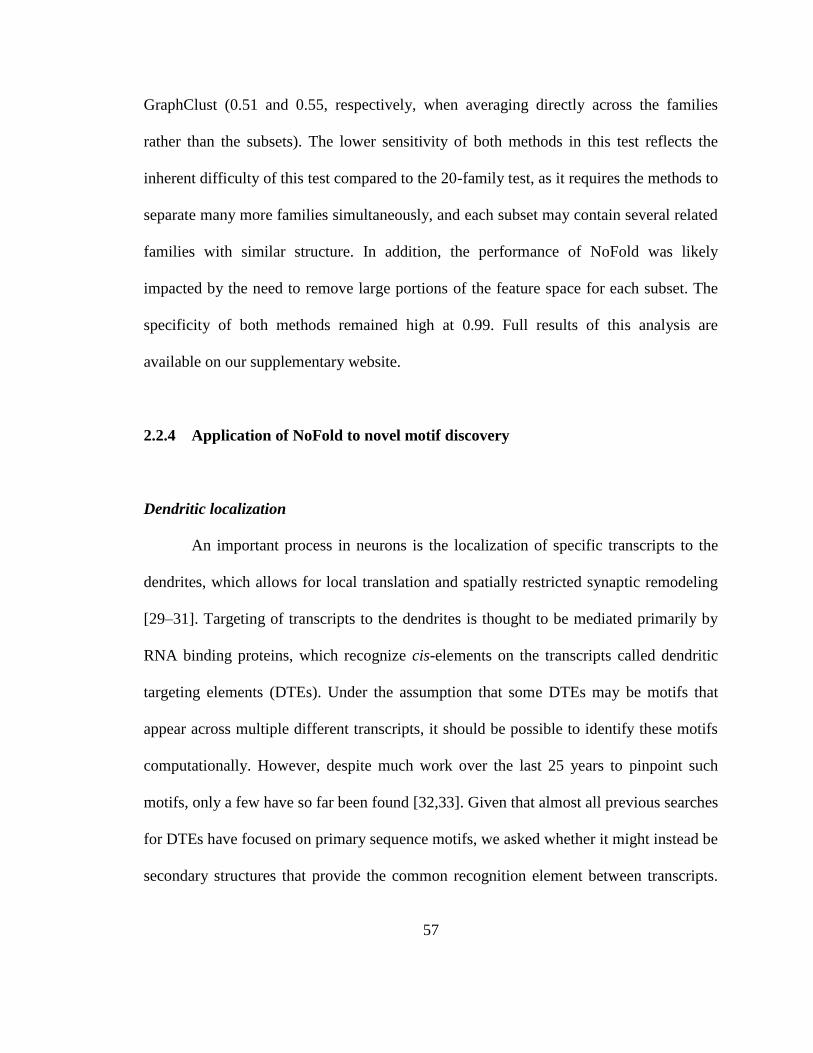
57
GraphClust (0.51 and 0.55, respectively, when averaging directly across the families
rather than the subsets). The lower sensitivity of both methods in this test reflects the
inherent difficulty of this test compared to the 20-family test, as it requires the methods to
separate many more families simultaneously, and each subset may contain several related
families with similar structure. In addition, the performance of NoFold was likely
impacted by the need to remove large portions of the feature space for each subset. The
specificity of both methods remained high at 0.99. Full results of this analysis are
available on our supplementary website.
2.2.4 Application of NoFold to novel motif discovery
Dendritic localization
An important process in neurons is the localization of specific transcripts to the
dendrites, which allows for local translation and spatially restricted synaptic remodeling
[29–31]. Targeting of transcripts to the dendrites is thought to be mediated primarily by
RNA binding proteins, which recognize cis-elements on the transcripts called dendritic
targeting elements (DTEs). Under the assumption that some DTEs may be motifs that
appear across multiple different transcripts, it should be possible to identify these motifs
computationally. However, despite much work over the last 25 years to pinpoint such
motifs, only a few have so far been found [32,33]. Given that almost all previous searches
for DTEs have focused on primary sequence motifs, we asked whether it might instead be
secondary structures that provide the common recognition element between transcripts.
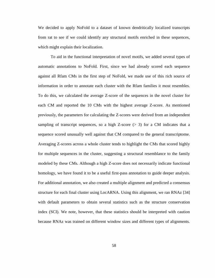
58
We decided to apply NoFold to a dataset of known dendritically localized transcripts
from rat to see if we could identify any structural motifs enriched in these sequences,
which might explain their localization.
To aid in the functional interpretation of novel motifs, we added several types of
automatic annotations to NoFold. First, since we had already scored each sequence
against all Rfam CMs in the first step of NoFold, we made use of this rich source of
information in order to annotate each cluster with the Rfam families it most resembles.
To do this, we calculated the average Z-score of the sequences in the novel cluster for
each CM and reported the 10 CMs with the highest average Z-score. As mentioned
previously, the parameters for calculating the Z-scores were derived from an independent
sampling of transcript sequences, so a high Z-score (> 3) for a CM indicates that a
sequence scored unusually well against that CM compared to the general transcriptome.
Averaging Z-scores across a whole cluster tends to highlight the CMs that scored highly
for multiple sequences in the cluster, suggesting a structural resemblance to the family
modeled by these CMs. Although a high Z-score does not necessarily indicate functional
homology, we have found it to be a useful first-pass annotation to guide deeper analysis.
For additional annotation, we also created a multiple alignment and predicted a consensus
structure for each final cluster using LocARNA. Using this alignment, we ran RNAz [34]
with default parameters to obtain several statistics such as the structure conservation
index (SCI). We note, however, that these statistics should be interpreted with caution
because RNAz was trained on different window sizes and different types of alignments.

59
Finally, we automatically trained a new CM for each final cluster which can be used in
the future to search additional databases for instances of the motifs.
As a first step towards identifying structural DTEs, we compiled a list of 211
transcripts with experimental evidence for dendritic localization in rat neurons. From
each transcript, we obtained from RefSeq (rn4) the 3’UTR sequence as well as the
sequence of any cytoplasmically retained introns [35], which have previously been shown
to harbor DTEs [36]. To focus our search on smaller structure elements, we used a sliding
window approach to split each 3’UTR and intron sequence into several smaller segments.
We have validated that the use of a sliding window still allows for good sensitivity of
motif detection (see supplementary website). We created 50nt and 150nt sliding window
sets for the retained intron and 3’UTR sequences of the dendritically localized transcripts
and searched these regions for motifs using NoFold (Table 2-3). NoFold identified a total
of 290 clusters (“motifs”) that contained three or more sequences. To test whether these
motifs were enriched within dendritic transcripts, we created a background datasets
consisting of introns or 3’UTRs (RefSeq, rn4) from non-dendritically localized
transcripts and scanned this set for matches to the NoFold motifs (see “Dendritic
localization dataset” in Methods). This was done using the cluster-CM for each motif in
conjunction with the cmsearch program [27]. We compared the number of motif matches
between the dendritic sequences and non-dendritic sequences and found a total of 213 of
the motifs were significantly enriched in the dendritic transcripts (Fisher’s exact test,
FDR-adjusted p < 0.05).
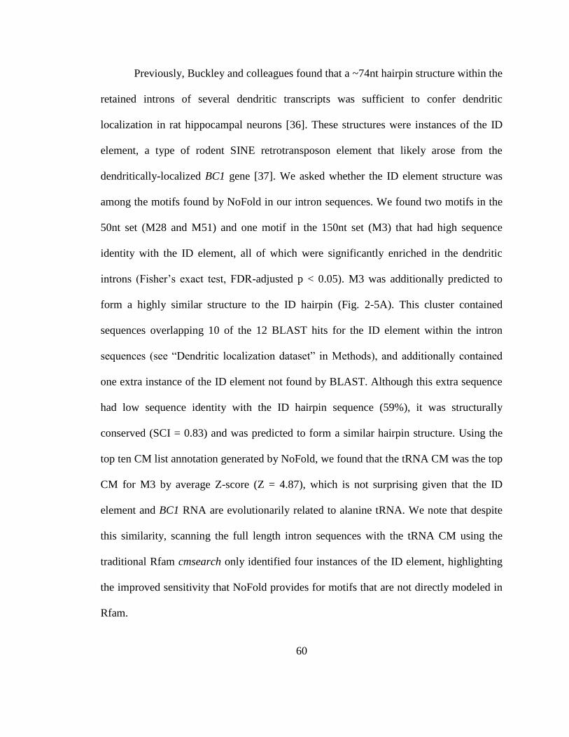
60
Previously, Buckley and colleagues found that a ~74nt hairpin structure within the
retained introns of several dendritic transcripts was sufficient to confer dendritic
localization in rat hippocampal neurons [36]. These structures were instances of the ID
element, a type of rodent SINE retrotransposon element that likely arose from the
dendritically-localized BC1 gene [37]. We asked whether the ID element structure was
among the motifs found by NoFold in our intron sequences. We found two motifs in the
50nt set (M28 and M51) and one motif in the 150nt set (M3) that had high sequence
identity with the ID element, all of which were significantly enriched in the dendritic
introns (Fisher’s exact test, FDR-adjusted p < 0.05). M3 was additionally predicted to
form a highly similar structure to the ID hairpin (Fig. 2-5A). This cluster contained
sequences overlapping 10 of the 12 BLAST hits for the ID element within the intron
sequences (see “Dendritic localization dataset” in Methods), and additionally contained
one extra instance of the ID element not found by BLAST. Although this extra sequence
had low sequence identity with the ID hairpin sequence (59%), it was structurally
conserved (SCI = 0.83) and was predicted to form a similar hairpin structure. Using the
top ten CM list annotation generated by NoFold, we found that the tRNA CM was the top
CM for M3 by average Z-score (Z = 4.87), which is not surprising given that the ID
element and BC1 RNA are evolutionarily related to alanine tRNA. We note that despite
this similarity, scanning the full length intron sequences with the tRNA CM using the
traditional Rfam cmsearch only identified four instances of the ID element, highlighting
the improved sensitivity that NoFold provides for motifs that are not directly modeled in
Rfam.

61
In addition to the ID element, we also identified several motifs with similarity to
known localization elements from Drosophila. Most strikingly, we found that 37 motifs
were annotated as having the K10 transport/localization element CM (K10_TLS;
RF00207) among their top ten best CMs, with five of these motifs having an average Z-
score > 5 and 28 having a Z-score > 3 for this CM. The K10_TLS is a 44nt hairpin
structure that mediates localization of the K10 mRNA during Drosophila oocyte
development [38]. The majority of our K10_TLS-like motifs were predicted to have a
stem-loop consensus structure enriched with AU base pairs (72% AU-content on
average), similar to K10_TLS (Fig. 2-5B), although primary sequence identity was low.
Overall, these 37 clusters encompassed a total of 60 unique genes, which is 28% of the
total genes in the datasets, and 28 of the clusters were significantly enriched in dendritic
transcripts (Fisher’s exact test, FDR-adjusted p < 0.05). We also found nine motifs with
another Drosophila localization structure, the Wingless localization element 3 (WLE3;
RF01046), within their top ten CMs, although only one had an average Z > 3. To our
knowledge, a role for these motifs has not yet been described in mammals. Additionally,
we identified several potentially novel motifs with stable and conserved structure, such as
hairpin motif M172, which is found in six dendritic transcripts, and double-hairpin motif
M158, which is found in four transcripts (Fig. 2-5C). Full data on all identified motifs are
available on our supplementary website.
Non-canonical translation initiation sites
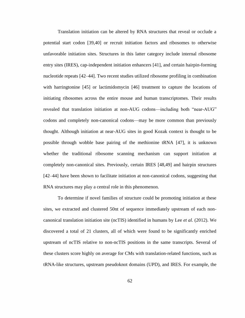
62
Translation initiation can be altered by RNA structures that reveal or occlude a
potential start codon [39,40] or recruit initiation factors and ribosomes to otherwise
unfavorable initiation sites. Structures in this latter category include internal ribosome
entry sites (IRES), cap-independent initiation enhancers [41], and certain hairpin-forming
nucleotide repeats [42–44]. Two recent studies utilized ribosome profiling in combination
with harringtonine [45] or lactimidomycin [46] treatment to capture the locations of
initiating ribosomes across the entire mouse and human transcriptomes. Their results
revealed that translation initiation at non-AUG codons—including both “near-AUG”
codons and completely non-canonical codons—may be more common than previously
thought. Although initiation at near-AUG sites in good Kozak context is thought to be
possible through wobble base pairing of the methionine tRNA [47], it is unknown
whether the traditional ribosome scanning mechanism can support initiation at
completely non-canonical sites. Previously, certain IRES [48,49] and hairpin structures
[42–44] have been shown to facilitate initiation at non-canonical codons, suggesting that
RNA structures may play a central role in this phenomenon.
To determine if novel families of structure could be promoting initiation at these
sites, we extracted and clustered 50nt of sequence immediately upstream of each non-
canonical translation initiation site (ncTIS) identified in humans by Lee et al. (2012). We
discovered a total of 21 clusters, all of which were found to be significantly enriched
upstream of ncTIS relative to non-ncTIS positions in the same transcripts. Several of
these clusters score highly on average for CMs with translation-related functions, such as
tRNA-like structures, upstream pseudoknot domains (UPD), and IRES. For example, the

63
top scoring CM for cluster T17 (Fig. 2-6) was the human heat shock protein 70 IRES (Z-
score = 3.8). Two tRNA-like structures (TLS), TLS-PK3 and TLS-PK2, were also within
the top ten best CMs for this cluster (Z = 2.8 and 2.7, respectively). The sequences in
cluster T1 (Fig. 2-6) scored highly against the CMs for two human IRES, the insulin-like
growth factor II IRES (Z = 2.5) and the fibroblast growth factor-2 IRES (Z = 2.0). In
addition, this cluster scored relatively highly against the tRNA-like TLS-PK4 (p = 8.9e-
9).
The largest cluster we found contained six sequences belonging to histone subunit
H4 genes, as well as one sequence belonging to heat shock protein 60. This cluster scored
highly for the L-myc IRES and is predicted to form a small hairpin (Cluster T6, Fig. 2-6).
Interestingly, H4 transcripts were recently shown in mouse to use an unusual mechanism
for translational initiation that involves loading of ribosomes independently of the 5’ cap
[50]. This process is thought to depend on two RNA structures, one that recruits the cap
binding protein eIF4E and another that may help position the ribosome over the initiation
site, similarly to an IRES. It has not yet been investigated whether this mechanism
supports initiation at non-canonical initiation codons. Several other histone genes were
found in other clusters, including two sequences from H2B in cluster T5 and two
sequences of H3 in cluster T13. To our knowledge, initiation at non-canonical codons has
not yet been investigated in these histone mRNAs.
Altogether, these results suggest that NoFold is useful as a first-pass high-
throughput screen to identify the locations of recurring structural motifs in a dataset,
64
which can then be used to prioritize sequences for lower-throughput experimental
analyses.
2.3 Discussion
We have described here a novel approach for clustering RNA secondary structures
that uses comparison to empirical models to map RNA sequences to a structural feature
space (the RESS). By scoring primary RNA sequences across a large number of Rfam
CMs and treating the scores as geometric coordinates, the RESS allows interpolation and
extrapolation across existing models to identify novel combinations of structural features
modeled by the original Rfam CMs. We find that sequences from the same structure
family tend to cluster within the RESS and that these clusters can be extracted from
unrelated sequences using unsupervised methods with very high sensitivity and precision.
We use our approach to identify 213 motifs enriched in dendritically localized transcripts
in rat. We hypothesize that some of these motifs may play a functionally important role in
dendritic localization given their enrichment within dendritic transcripts and, for several
motifs, high scores for CMs related to localization.
Within the dendritic RNAs we identified a large number of clusters that scored
highly against the K10_TLS CM. It is unclear whether these clusters represent distinct
structure families or are subgroups of one larger structure family that might include
K10_TLS. Early studies of the K10_TLS indicated that the size and shape of the structure
were most important for localization and that most nucleotides in the stem and loop
regions can be changed as long as they do not disrupt base pairing [38]. More recently, a

65
tertiary structure analysis of K10_TLS by NMR spectroscopy revealed that extensive
purine stacking within the AU-rich stem region causes K10_TLS to take on an A’-form
helix conformation with a widened major groove, and that this geometry is important for
localization [51]. Although tertiary features such as this are not directly modeled by CMs
and therefore may not be captured by our method, it is possible that the high AU content
found in most of our K10_TLS-like motifs could allow them take on an A’-form helix
and therefore be localized by a similar mechanism. As these results are still preliminary,
additional experiments will be needed to verify these motifs and identify which proteins
recognize them.
Of the 21 structure clusters found upstream of human ncTIS, all contained seven
or fewer sequences, indicating that no single structure accounts for a large portion of
human non-canonical initiation. A possible complicating factor in this analysis is that
initiation-promoting motifs do not necessarily occur immediately upstream of the ncTIS.
Some IRES are located distally from the start codon and interact with the initiation site
by pseudoknot formation [49]. This makes it difficult to find motifs specifically involved
in non-canonical initiation, since one must link the distal motif with the ncTIS using
either pseudoknot prediction, which is computationally intensive for long sequences, or
direct experimental probing. Therefore, we expect that our analysis of only the regions
upstream of ncTIS is an underestimation of the motifs involved in non-canonical
initiation. In some cases, small hairpin structures located immediately upstream of
initiation sites have been shown to help mediate pseudoknot interactions. The Cricket
paralysis virus (CrPV) IRES, for example, utilizes a pseudoknot between an ncTIS and a

66
slightly upstream tRNA-like hairpin to cause translation initiation in the absence of
initiation factors (including tRNA-Met) [48,49]. Hairpins such as this should be
detectable by our analysis, provided they are within the 50nt upstream window used here,
and in fact we did obtain several clusters with strong hits for tRNA-like structures and
hairpins (e.g. cluster T17 in Fig. 2-6B). It is possible that as more ncTIS are discovered,
more instances of these motifs will be found.
Beyond the experimental dataset considered here, there are many possible
applications of NoFold. For example, to identify structures bound by a particular RNA-
binding protein, one could analyze sequences that are known to be bound by that protein
to see if any common motifs emerge. A similar tactic could be applied to find motifs
involved in splicing, RNA stability, and translational efficiency. The RESS itself could
also be used directly as a feature space for supervised classification of RNAs, e.g.
classification of unannotated non-coding RNAs into broad functional categories, as has
been attempted using other types of features [52].
We note that since the scoring process scales linearly with increasing dataset size,
this approach is feasible for datasets up to several thousand sequences. Specifically, on
one CPU core, a single 50nt sequence was scored in an average of 0.012s per CM, or
~24s for the entire Rfam CM set. Since the scaling for increasing sequence lengths is
quadratic, we generally recommend using sequences or sliding windows of < 300nt. We
have implemented an option to parallelize the scoring process and several of the
downstream steps of NoFold, which can greatly decrease runtime when the appropriate
hardware is available. Runtime for the downstream steps of the NoFold process generally

67
depended on the number of clusters that passed the thresholds, but usually took
substantially less time than scoring. Although the overall runtime of GraphClust was
generally shorter than NoFold on a single core (3 minutes for GraphClust vs. 39 minutes
for NoFold on a 100-sequence dataset), NoFold was sped up considerably when
parallelized (4.2 minutes on 16 cores for the same dataset). In contrast, we observed that
GraphClust did not always make use of all available cores (2.2 minutes on 16 cores for
the same dataset). This appears to be dependent on the number of clusters that were
actually found.
An important limitation of our approach can arise from the use of empirical
models to construct the feature space. An ideal set of empirical models should comprise
all of the major structures of RNA such that any RNA structure can be placed “inside”
the coordinates. By using all available models, we hoped to create such a feature space,
but we do not have any guarantee. Another remaining limitation of our method is the
detection of structures embedded in larger sequences. Here we used a sliding window to
segment larger sequences to aid in detecting such structures, at the expense of some
sensitivity. More sophisticated methods that might optimize for subsequence structures
will yield improvements in this area. The development of alternate methods for
segmenting large sequences will likely continue to improve the sensitivity of NoFold and
other existing motif finders. Another avenue for improvement is in cluster delineation.
Here we developed several data-driven criteria for cluster identification, but many other
machine learning approaches may be applied to the basic concept of RESS.

68
An interesting future consideration will be the tailoring of different collections of
empirical models to suit specific applications. Although here we used the entire set of
Rfam v.10.1 CMs to define our feature space, different utility might be found using
different subsets of CMs (or other models). As discussed in the introduction and results,
the coordinate space established by the RESS using the CMs may be seen as a set of
canonical models against which novel sequences are compared to assess their inter-
relationships. We hypothesize that if the models are at large scale (e.g., a sparse set of
very different secondary structures), this is akin to having very coarse-grained models
and such a subset of models (i.e., CMs) may be useful for large scale structure
discrimination but not for fine-scaled differences. Alternatively, we hypothesize that a set
of closely related CMs may help discriminate fine-scaled differences. Thus, future work
may entail using different subsets of CMs and resulting RESS coordinates for different
subgroups of structures.
2.4 Methods
Data and Software
NoFold is available on our website, kim.bio.upenn.edu/software/nofold.shtml.
Full clustering results and input datasets used in this study are also available on the site.
Scoring of RNA sequences
69
Sequences were scored against each of the 1,973 Rfam CMs (v.10.1) using the
cmscore module of Infernal (v.1.0.2) with options “--search --a” [27].
Normalization of feature space
To obtain normalization parameters, a dataset was generated by extracting
sequences of varying length from random locations within transcripts sampled from the
whole mouse (UCSC, mm9) and human (RefSeq, hg19) transcriptomes. Any exactly
identical sequences were removed. We included 50 sequences of each length in the range
of 10-500nt in the dataset, for a total of 24,550 sequences. We used this dataset to obtain
the parameters for normalization and standardization of the feature space that were used
for all other datasets. First, for each CM, we estimated the mean and standard deviation
of scores obtained by sequences of each length. We used these parameters to Z-score
sequences in a length- and CM-dependent manner, as described in the text. Next, after
normalizing the scores of the 24,550 sequences in this manner, we performed PCA (using
prcomp in R) on the dataset to obtain a set of independent axes. We retained only the
axes with an eigenvalue greater than 1.0 (Kaiser criterion), which yielded 124 axes. We
rounded this down to the top 100 axes and recorded the loadings for these axes to use for
future datasets. Finally, we recorded a set of parameters to re-standardize the 100 PC
axes. All subsequent datasets were mapped to this normalized feature space (the RESS)
using the parameters estimated here.
Synthetic structures
70
We designed the following synthetic structures, which we show below in dot-
bracket notation (where matching parentheses represent paired bases and periods
represent unpaired bases):
1-hp: (((((((((((((((((((((((((((((((((.....)))))))))))))))))))))))))))))))))
2-hp: (((((((((((((((((((((((.....)))))))))))))((((((((....))))))))))))))))))
3-hp: (((((((((((((((((((....)))))(((((.....)))))(((((....)))))))))))))))))))
Two-dimensional representations of these structures are also shown in Fig. 2-2A. We
randomly generated 50 sequences for each structure by generating complementary base
pairs simultaneously (but randomly) as defined in the dot-bracket string. This ensured
that each sequence had at least the potential to form the exact intended structure. Only
Watson-Crick base pairs (A-U and G-C) were used. G-U wobble pairs were not used for
simplicity. We did not require that the MFE structure be equivalent to the intended
structure, although we note that the majority of the sequences did form the intended
structure when folded by RNAFold.
To test distance measures, we generated all possible pairs of sequences from the
same structure, different structures, or random sequences (which may or may not have
stable structure). For each pair of sequences, we measured their percent sequence identity
and their Spearman distance within the RESS, where Spearman distance is defined as one
minus the Spearman correlation of the coordinates of the two sequences in the RESS. The
random sequences were generated to have the same average di-nucleotide frequency as
the structural sequences but had no particular structure. Average di-nucleotide frequency
was matched by generating sequences according to a first-order Markov process where
71
the transition probability between each pair of nucleotides was estimated from the
sequences of the original dataset.
NoFold structure clustering pipeline
A procedure to delineate robust RNA sequence clusters in the structural feature
space was implemented as follows. Scored sequences were clustered by hierarchical
clustering (average linkage using Spearman distance) using the fastcluster package [28]
in R. Using a procedure similar to that described in [53], the resulting dendrogram was
cut into all possible clusters of size three or greater and the average pairwise Spearman
distance between cluster members was calculated for each cluster (cluster “diameter”);
then any clusters with a diameter larger than an empirically derived threshold were
removed (see Threshold Determination, below). Since cutting the dendrogram into all
possible clusters results in many clusters that contain almost the same sequences, we
implemented two filters for choosing non-overlapping clusters: a “sensitive” filter
(optimized for picking larger clusters) and a “specific” filter (optimized for picking
tighter clusters). In the sensitive filter, clusters are first ranked by their size (large to
small) and then by their diameter (small to large). Clusters were then chosen in a greedy
manner from first to last, throwing out any clusters that overlap with a previously chosen
cluster. In the specific filter, clusters with three or more members were simply ranked by
diameter (small to large) and then chosen greedily as above. We tested these two filters
using sequences from the BRAliBase II benchmark datatset [11] and found that the
specific filter produced fewer false positives but sometimes missed positive examples. To

72
improve the sensitivity of this mode without sacrificing specificity, we implemented an
additional cluster-expansion step, where a new CM was trained for each cluster (“cluster-
CM”) based on the multiple alignment of the cluster sequences by LocARNA. These
cluster-CMs were then used to pick up additional matches to the structure within the
original sequence database using the cmsearch module of Infernal with options “--
toponly --glocal”. A sequence was counted as a hit for a given cluster-CM if it obtained a
bitscore of at least log2(size of search database), or in the case of the dendritic and non-
canonical translation datasets, a bitscore of at least 10. If any two expanded clusters
overlapped by more than 50%, they were merged into one cluster. After cluster expansion
and merging, each cluster was automatically annotated in several ways to help give
insight into potential functions, as described in the text. RNAz was run using default
parameters.
Threshold determination
An empirical threshold for filtering clusters based on diameter (average pairwise
Spearman distance) was calculated based on the distribution of cluster diameters that
result from clustering random, unrelated sequences. Since the expected cluster diameter
is dependent on the total number of sequences in the dataset being clustered, we
separately calculated this threshold for different database sizes (usually rounding the
database size to the nearest 100). For a given dataset size, we also calculated a separate
threshold for each cluster size (where size refers to the number of cluster members), since
clusters with more members tend to have larger diameters.
73
We created a dataset of 10,000 random 50nt sequences with the same average di-
nucleotide frequency as the mouse and human transcriptomes using a first-order Markov
model as described in the “Synthetic Structures” section. Since these sequences were
randomly generated, we do not expect them to share substantial structure. Sequences
were scored and mapped to the RESS. To obtain the distribution of cluster diameters for a
given dataset size, we used the following procedure: (1) a subset of the 10,000 sequences
was picked at random to create a dataset of the desired size; (2) the subset was
hierarchically clustered using Spearman distances and average linkage and all possible
clusters were extracted from the resulting dendrogram; (3) the diameter of each cluster
was calculated and recorded in separate lists based on the number of sequences in the
cluster; (4) steps 1-3 were repeated enough times to obtain >10,000 observations of
clusters of size three (this required more iterations for small datasets and fewer for large
datasets). The result of this procedure was a distribution of cluster diameters for each size
cluster. A “high-confidence” threshold for each cluster size was then defined as the
distance at which 99% of the clusters of that size had a larger diameter than the threshold,
and a “good-confidence” threshold was set at the 95% mark. At these thresholds, we
would expect about 1% and 5% of structurally unrelated clusters to pass the thresholds,
respectively. The 95% threshold was used for choosing clusters in all analyses described
here.
Rfam benchmark tests
74
RNA sequences were taken from the Rfam.seed file available on the Rfam FTP
(v.10.1). This file contains sequences from the seed alignments of 1,973 Rfam families.
We extracted the sequences for the first 20 Rfam families (RF00001-RF00020) and
filtered each family so that no pair of sequences had more than 75% sequence identity.
Sequence identity was calculated using the alignments specified in the Rfam.seed file,
which is a multiple alignment of the whole family. Insertion characters (e.g. “.”) were
therefore ignored if they were present in both sequences being compared. After the
sequence identity filtering, all remaining sequences in the family were used as part of the
benchmark, up to a maximum of 100 sequences per family. Family RF00014 (DsrA) had
only one sequence left after filtering (of the original five) and was therefore replaced by
RF00032 (Histone3), which was chosen because it is often used in the literature as a
structure analysis benchmark family and is a particularly small structure. Altogether, this
yielded a dataset of 978 sequences. All information about alignment was removed,
including all non-nucleotide characters. We referred to this dataset as the “plain
sequences”. We additionally generated an “embedded sequence” dataset and a “plain
sequences with background” dataset. The embedded dataset was created by adding 10-
50nt (amount randomly chosen) of additional flanking sequence to both the 5’ and 3’
ends of each sequence in the plain dataset. The flanking sequence was matched to the
average mono-nucleotide frequency of the plain sequence dataset. The background-
containing dataset consisted of the plain dataset with an additional 3,000 random
sequences mixed in, such that the random sequences outnumbered the Rfam sequences
~3:1. These sequences were generated to have the same average di-nucleotide frequency
75
as the plain dataset to ensure that di-nucleotide frequency alone was not sufficient to
cause clustering of random sequences. Matching of the average di-nucleotide frequency
was performed using a first-order Markov process, as described in the “Synthetic
structures” section.
After scoring but before clustering, we examined the sequences of each family for
particularly high scores against the feature space CMs. We identified all CMs that had an
average Z-score > 3 (as calculated using the Z-score parameters described in the
“Normalization of feature space” section) and removed these CMs from the RESS. This
also required us to re-estimate the RESS PCA projection without these CMs. The full list
of CMs that were removed is: 5S_rRNA, 5_8S_rRNA, U1, U2, tRNA, tRNA-Sec,
Tymo_tRNA-like, mascRNA-menRNA, tmRNA, Vault, U12, Bacteria_large_SRP,
Hammerhead_1, Hammerhead_3, RNaseP_nuc, RNase_MRP, RNaseP_arch,
RNaseP_bact_a, RNaseP_bact_b, ACEA_U3, Fungi_U3, Plant_U3, U3, 6S, U4, U4atac,
SNORD14, SNORD53_SNORD92, Archaea_SRP, Bacteria_small_SRP, DdR20,
Fungi_SRP, Metazoa_SRP, Plant_SRP, Protozoa_SRP, CsrB, CsrC, PrrB_RsmZ, RsmY,
mir-299, Y_RNA, ceN72-3, U5, Histone3. Linear discriminant analysis was performed
using the MASS package in R, and the top loaded CM for each axis was examined
manually. A list of the loadings obtained in this analysis is available on the
supplementary website.
NoFold and GraphClust were run on each of the three datasets using default
parameters, with the exception that sliding window generation was turned off for
GraphClust to make the results more easily compared. It is possible that the use of a

76
sliding window with both approaches could improve performance. Although GraphClust
has many parameters that could potentially be tuned to produce better results, we felt that
the default parameters were reasonable for the purposes of this test. In particular, the
default specifies that GraphClust will be run for two iterations and find up to 10 clusters
per iteration, which is theoretically sufficient to identify the 20 expected clusters in this
particular dataset. Our results should be interpreted as how each method performs “out-
of-the-box”, without tuning of parameters or use of a prioi knowledge of the size or
number of motifs.
Rfam families were grouped for the cross-validation analysis by clustering all of
the 1,973 CMs based on their scores against a large set of random transcripts (same
dataset as described in “Normalization of feature space” above). Hierarchical clustering
using Spearman distance and Ward linkage was used. The dendrogram was cut at a
height such that exactly 10 clusters were created by the cut. The CMs in each cluster then
determined which families were grouped together for the analysis. The reason for
clustering the families in this way was to reduce the number of CM features that had to
be removed for each analysis. GraphClust was set to run for 25 iterations (10 clusters per
iteration) for this analysis to ensure enough clusters could be detected in each subset.
NoFold was run using default parameters.
Dendritic localization dataset
Dendritic transcripts in rat hippocampal neurons were identified by in situ
hybridization and soma-/dendrite-specific microarrays (unpublished data from J. Kim

77
lab). A transcript was called “dendritically localized” if it had high expression in the
dendrites relative to the soma in either the in situ or microarray analysis, yielding 182
dendritically localized transcripts. An additional 29 known dendritically localized
transcripts in rodents were obtained from [54]. Sequences from the 3’UTR of these
transcripts were obtained from RefSeq annotations (rn4) using the UCSC genome
browser. If more than one 3’UTR was available for a given gene, only the longest
sequence was used. Cytoplasmically retained intron sequence were identified in rat using
RNA-seq [35] and those belonging to a dendritically localized transcript were used for
the dataset. These sequences consisted only of the regions of the intron that were
supported by reads, as described in [35]. Since intron and 3’UTR sequences are long and
may contain multiple structures, we generated a sliding window datasets for each using a
50nt window with a 35nt slide or a 150nt with a 105nt slide. Instances of the ID element
within the intron dataset were identified by a BLASTn search of the full length retained
intron sequences using the default parameters on the BLAST website [55].
As a background dataset, we identified a set of non-dendritically targeted
transcripts based on their very low expression in dendrites relative to the soma from the
microarray analysis. Introns and 3’ UTR sequences were extracted for a random subset of
the top 1000 non-dendritic transcripts and processed as above to create background
datasets of 10,000-30,000 windows for each analysis. The GC content of the background
datasets was 44-48%, which was similar to the test sequences (43-45% GC). To test a
motif for enrichment within the dendritically localized set, we generated a cluster-CM for
each final motif using cmbuild [27] and used this to search the background dataset as well
78
as the original dataset. The number of hits in each dataset was used in a one-sided
Fisher’s exact test for enrichment of hits in the dendritic set, and Benjamini-Hochberg
multiple testing correction was applied using R.
Translation initiation dataset
The transcript positions of non-canonical translation initiation sites (ncTIS) in
mouse and human were obtained from Lee et al. [46]. Codons were defined as ncTIS if
they were neither AUG nor near-AUG codons but showed translation initiation through
ribosome profiling analysis. Since multiple mapping of non-unique ribosome footprints
was allowed in the original dataset, we removed any ncTIS that was surrounded by >20nt
of sequence that was exactly identical to any other ncTIS. Such ncTIS mostly fell within
repetitive elements. We extracted 50nt upstream of each remaining ncTIS, allowing the
extracted sequences to overlap by no more than 25nt. If such an overlap occurred, only
the first sequence was kept. If 50nt could not be extracted due to an ncTIS falling too
close to the 5’ end, the 5’ end was buffered with random sequence. A background
database for the enrichment analysis was created from 50nt upstream of random
transcript locations that were not within 25nt of an ncTIS. Only transcripts that had
observed expression in the ribosome profiling experiment were used to obtain
background sequences.
Figure generation

79
Plots were generated in R (www.r-project.org) using the ggplot2 package
(ggplot2.org). Structure depictions were created using VARNA [56] based on consensus
structure and sequence predictions from LocARNA.

80
Figure 2-1. Normalization of the empirical feature space.
Examples of CM score characteristics before (A,B) and after (C,D) normalization, for
sequences and CMs of length ≤ 500nt. (A) A representative example of the scores given
to sequences of various lengths against a single CM, in this case tRNA. We consistently
observe a relationship between sequence length and score that is most pronounced for
sequences that are smaller than the size of the CM (73nt in this case, indicated by the
dashed line). Gray lines show separate linear regression fits to the scores of sequences
shorter or longer than 73nt, with slopes (m) indicated. (B) We additionally observed a
relationship between the length of a CM and the average score that it produces. Average
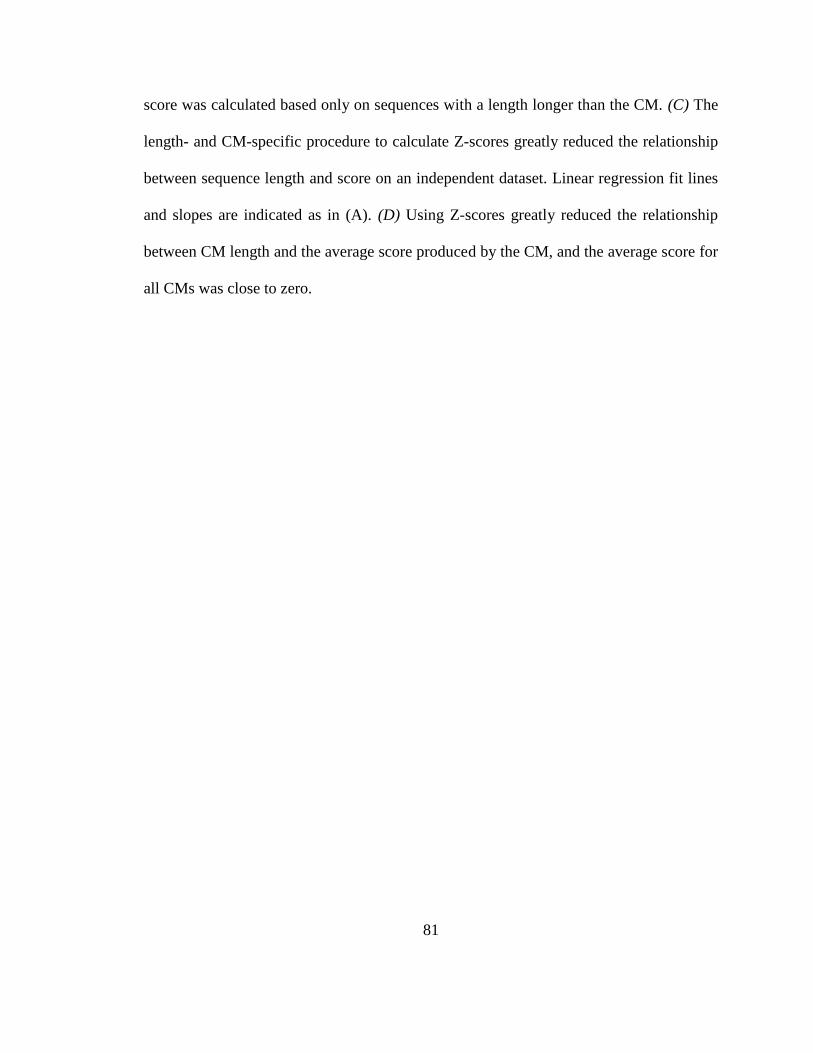
81
score was calculated based only on sequences with a length longer than the CM. (C) The
length- and CM-specific procedure to calculate Z-scores greatly reduced the relationship
between sequence length and score on an independent dataset. Linear regression fit lines
and slopes are indicated as in (A). (D) Using Z-scores greatly reduced the relationship
between CM length and the average score produced by the CM, and the average score for
all CMs was close to zero.

82
Figure 2-2. Structurally similar sequences are clustered together in the RESS.
(A) Three synthetic structures designed for this analysis. (B) PCA of the structure
sequences after projection to the RESS separates the sequences based on structure. (C)
Distributions of the distances between pairs of related structure (“1-hp vs 1-hp”, “2-hp vs
2-hp”, “3-hp vs 3-hp”), pairs of different structure (“Diff structs”), and pairs of random
sequences (“Rand vs Rand”). Distance between pairs was calculated by Spearman
distance (left panel) or sequence identity (right panel). Related structure pairs were
closer, on average, than different or random pairs in the RESS.
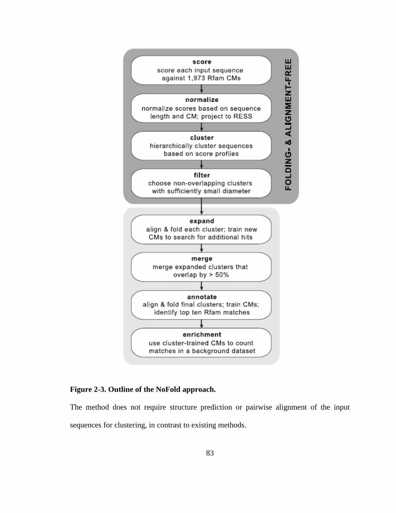
83
Figure 2-3. Outline of the NoFold approach.
The method does not require structure prediction or pairwise alignment of the input
sequences for clustering, in contrast to existing methods.

84
Figure 2-4. Distribution of the number of separate clusters assigned to each Rfam
family for a given test.
Clusters were assigned to a family only if it was the dominant family within that cluster.
The observations for all 20 families across all three tests are displayed. Most families
were assigned to only one cluster per test, and the maximum number of clusters per
family in any test was three.
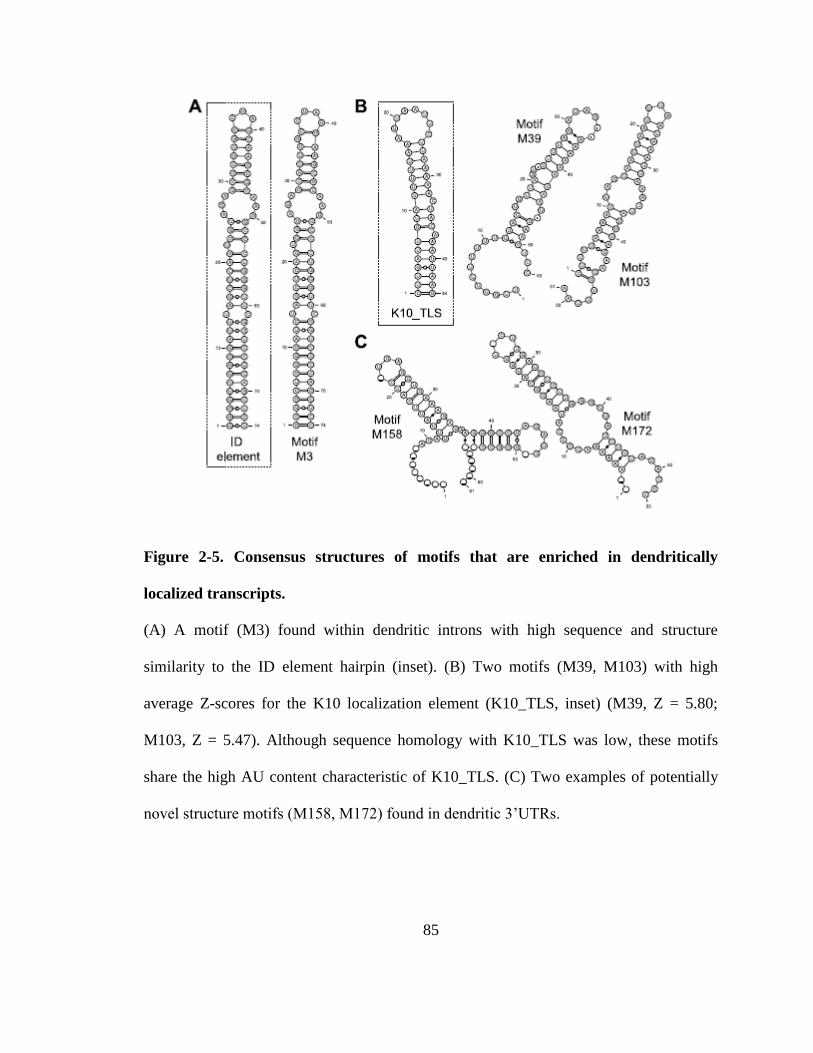
85
Figure 2-5. Consensus structures of motifs that are enriched in dendritically
localized transcripts.
(A) A motif (M3) found within dendritic introns with high sequence and structure
similarity to the ID element hairpin (inset). (B) Two motifs (M39, M103) with high
average Z-scores for the K10 localization element (K10_TLS, inset) (M39, Z = 5.80;
M103, Z = 5.47). Although sequence homology with K10_TLS was low, these motifs
share the high AU content characteristic of K10_TLS. (C) Two examples of potentially
novel structure motifs (M158, M172) found in dendritic 3’UTRs.
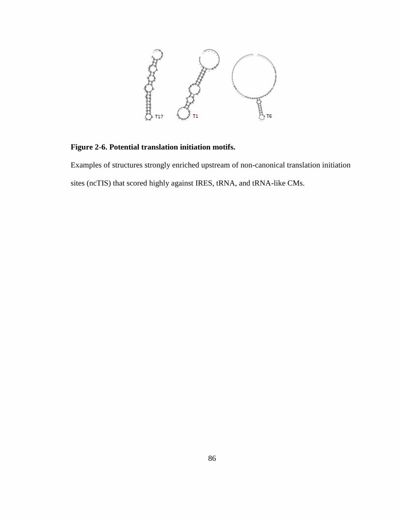
86
Figure 2-6. Potential translation initiation motifs.
Examples of structures strongly enriched upstream of non-canonical translation initiation
sites (ncTIS) that scored highly against IRES, tRNA, and tRNA-like CMs.
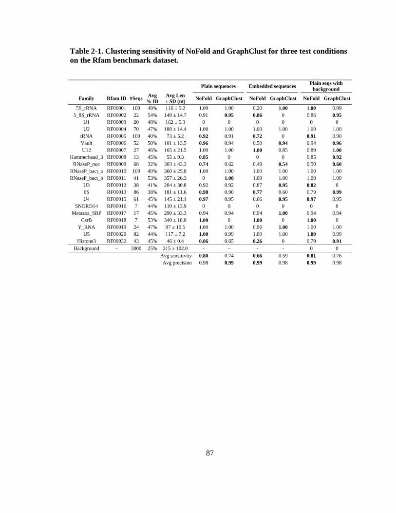
87
Table 2-1. Clustering sensitivity of NoFold and GraphClust for three test conditions
on the Rfam benchmark dataset.
Plain sequences
Embedded sequences Plain seqs with
background
Family Rfam ID #Seqs Avg
% ID
Avg Len
± SD (nt)
NoFold GraphClust
NoFold GraphClust
NoFold GraphClust
5S_rRNA RF00001 100 49% 116 ± 5.2 1.00 1.00 0.20 1.00 1.00 0.99
5_8S_rRNA RF00002 22 54% 149 ± 14.7 0.91 0.95 0.86 0 0.86 0.95
U1 RF00003 20 48% 162 ± 5.3 0 0 0 0 0 0
U2 RF00004 70 47% 188 ± 14.4 1.00 1.00 1.00 1.00 1.00 1.00
tRNA RF00005 100 40% 73 ± 5.2 0.92 0.91 0.72 0 0.91 0.90
Vault RF00006 52 50% 101 ± 13.5 0.96 0.94 0.50 0.94 0.94 0.96
U12 RF00007 27 46% 165 ± 21.5 1.00 1.00 1.00 0.85 0.89 1.00
Hammerhead_3 RF00008 13 45% 55 ± 9.3 0.85 0 0 0 0.85 0.92
RNaseP_nuc RF00009 68 32% 303 ± 43.3 0.74 0.62 0.49 0.54 0.50 0.60
RNaseP_bact_a RF00010 100 49% 360 ± 25.8 1.00 1.00 1.00 1.00 1.00 1.00
RNaseP_bact_b RF00011 41 53% 357 ± 26.3 0 1.00 1.00 1.00 1.00 1.00
U3 RF00012 38 41% 204 ± 30.8 0.92 0.92 0.87 0.95 0.82 0
6S RF00013 86 38% 181 ± 11.6 0.98 0.90 0.77 0.60 0.79 0.99
U4 RF00015 61 45% 145 ± 21.1 0.97 0.95 0.66 0.95 0.97 0.95
SNORD14 RF00016 7 44% 110 ± 13.9 0 0 0 0 0 0
Metazoa_SRP RF00017 17 45% 290 ± 33.3 0.94 0.94 0.94 1.00 0.94 0.94
CsrB RF00018 7 53% 340 ± 18.0 1.00 0 1.00 0 1.00 0
Y_RNA RF00019 24 47% 97 ± 10.5 1.00 1.00 0.96 1.00 1.00 1.00
U5 RF00020 82 44% 117 ± 7.2 1.00 0.99 1.00 1.00 1.00 0.99
Histone3 RF00032 43 45% 46 ± 0.4 0.86 0.65 0.26 0 0.79 0.91
Background - 3000 25% 215 ± 102.0 - - - - 0 0
Avg sensitivity 0.80 0.74 0.66 0.59 0.81 0.76
Avg precision 0.98 0.99 0.99 0.98 0.99 0.98

88
Table 2-2. Clustering sensitivity and precision of NoFold and GraphClust for the
synthetic structure benchmark.
NoFold GraphClust
Family # Seqs Avg % ID Length
(nt)
Sensitivity Precision
Sensitivity Precision
1-hairpin structure 50 25% 71 0.70 0.80 1.00 0.39
2-hairpin structure 50 25% 71 0.88 0.79 1.00 0.67
3-hairpin structure 50 25% 71 0.58 0.85 0 -
Average 0.72 0.81 0.67 0.53
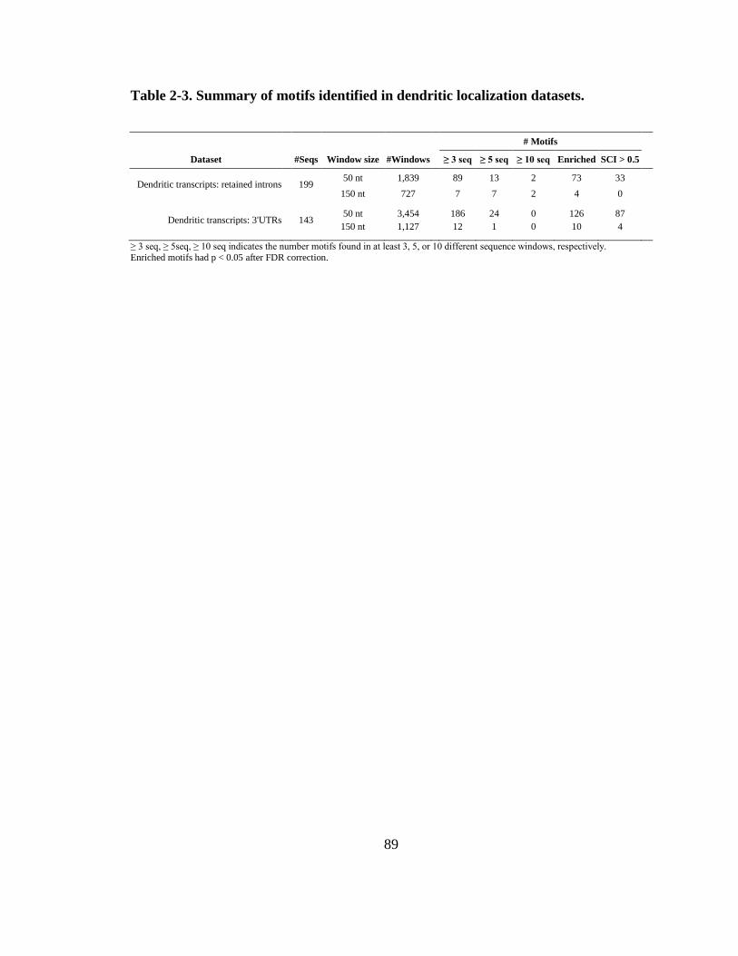
89
Table 2-3. Summary of motifs identified in dendritic localization datasets.
# Motifs
Dataset
#Seqs Window size #Windows
≥ 3 seq ≥ 5 seq ≥ 10 seq Enriched SCI > 0.5
Dendritic transcripts: retained introns
199 50 nt 1,839
89 13 2 73 33
150 nt 727
7 7 2 4 0
Dendritic transcripts: 3'UTRs
143 50 nt 3,454
186 24 0 126 87
150 nt 1,127
12 1 0 10 4
≥ 3 seq, ≥ 5seq, ≥ 10 seq indicates the number motifs found in at least 3, 5, or 10 different sequence windows, respectively.
Enriched motifs had p < 0.05 after FDR correction.
90
2.5 References
1 Wan, Y. et al. (2011) Understanding the transcriptome through RNA structure.
Nat. Rev. Genet. 12, 641–655
2 Walczak, R. et al. (1996) A novel RNA structural motif in the selenocysteine
insertion element of eukaryotic selenoprotein mRNAs. RNA 2, 367–79
3 Casey, J.L. et al. (1988) Iron-responsive elements: regulatory RNA sequences that
control mRNA levels and translation. Science 240, 924–8
4 Martin, K.C. and Ephrussi, A. (2009) mRNA Localization: Gene Expression in the
Spatial Dimension. Cell 136, 719–730
5 Burge, S.W. et al. (2012) Rfam 11.0: 10 years of RNA families. Nucleic Acids
Res. 41, 1–7
6 Eddy, S.R. and Durbin, R. (1994) RNA sequence analysis using covariance
models. Nucleic Acids Res. 22, 2079–2088
7 Zuker, M. (1989) On finding all suboptimal foldings of an RNA molecule. Science
244, 48–52
8 Zuker, M. (2003) Mfold web server for nucleic acid folding and hybridization
prediction. Nucleic Acids Res. 31, 3406–3415
9 Hofacker, I.L. (2003) Vienna RNA secondary structure server. Nucleic Acids Res.
31, 3429–3431
10 Hofacker, I.L. et al. (1994) Fast folding and comparison of RNA secondary
structures. Monatshefte fur Chemie Chem. Mon. 125, 167–188
11 Gardner, P.P. et al. (2005) A benchmark of multiple sequence alignment programs
upon structural RNAs. Nucleic Acids Res. 33, 2433–9
12 Torarinsson, E. et al. (2007) Multiple structural alignment and clustering of RNA
sequences. Bioinformatics 23, 926–32
13 Mathews, D.H. and Turner, D.H. (2002) Dynalign: an algorithm for finding the
secondary structure common to two RNA sequences. J. Mol. Biol. 317, 191–203
14 Will, S. et al. (2007) Inferring noncoding RNA families and classes by means of
genome-scale structure-based clustering. PLoS Comput. Biol. 3, e65
15 Sankoff, D. (1985) Simultaneous solution of the RNA folding, alignment and
protosequence problems. SIAM J. Appl. Math. 45, 810–825
16 Ding, Y. et al. (2005) RNA secondary structure prediction by centroids in a
Boltzmann weighted ensemble. RNA 11, 1157–1166
17 Liu, Q. et al. (2008) RNACluster: An integrated tool for RNA secondary structure
comparison and clustering. J. Comput. Chem. 29, 1517–1526
91
18 Moulton, V. et al. (2000) Metrics on RNA secondary structures. J. Comput. Biol.
7, 277–92
19 Höchsmann, M. et al. (2004) Pure multiple RNA secondary structure alignments: a
progressive profile approach. IEEE/ACM Trans. Comput. Biol. Bioinform. 1, 53–
62
20 Liu, J. et al. (2005) A method for aligning RNA secondary structures and its
application to RNA motif detection. BMC Bioinformatics 6, 89
21 Steffen, P. et al. (2006) RNAshapes: an integrated RNA analysis package based on
abstract shapes. Bioinformatics 22, 500–3
22 Yao, Z. et al. (2006) CMfinder--a covariance model based RNA motif finding
algorithm. Bioinformatics 22, 445–52
23 Heyne, S. et al. (2012) GraphClust: alignment-free structural clustering of local
RNA secondary structures. Bioinformatics 28, i224–i232
24 Scholkopf, B. and Mika, S. (1999) Input space versus feature space in kernel-based
methods. IEEE Trans. Neural Netw. 10, 1000–1017
25 Moore, S.D. and Sauer, R.T. (2007) The tmRNA system for translational
surveillance and ribosome rescue. Annu. Rev. Biochem. 76, 101–24
26 Jan, E. et al. (2003) Divergent tRNA-like element supports initiation, elongation,
and termination of protein biosynthesis. Proc. Natl. Acad. Sci. U. S. A. 100,
15410–15415
27 Nawrocki, E.P. et al. (2009) Infernal 1.0: inference of RNA alignments.
Bioinformatics 25, 1335–7
28 Müllner, D. (2011) fastcluster: Fast Hierarchical, Agglomerative Clustering
Routines for R and Python. J. Stat. Softw. 53,
29 Job, C. and Eberwine, J. (2001) Localization and translation of mRNA in dendrites
and axons. Nat. Rev. Neurosci. 2, 889–898
30 Sutton, M.A. and Schuman, E.M. (2006) Dendritic protein synthesis, synaptic
plasticity, and memory. Cell 127, 49–58
31 Bramham, C.R. and Wells, D.G. (2007) Dendritic mRNA: transport, translation
and function. Nat. Rev. Neurosci. 8, 776–789
32 Eberwine, J. et al. (2002) Analysis of subcellularly localized mRNAs using in situ
hybridization, mRNA amplification, and expression profiling. Neurochem. Res. 27,
1065–77
33 Holt, C.E. and Schuman, E.M. (2013) The Central Dogma Decentralized: New
Perspectives on RNA Function and Local Translation in Neurons. Neuron 80,
648–657
34 Washietl, S. et al. (2005) Fast and reliable prediction of noncoding RNAs. Proc.
Natl. Acad. Sci. 102, 2454–2459
92
35 Khaladkar, M. et al. (2013) Subcellular RNA sequencing reveals broad presence of
cytoplasmic intron-sequence retaining transcripts in mouse and rat neurons. PLoS
One 8, e76194
36 Buckley, P.T. et al. (2011) Cytoplasmic intron sequence-retaining transcripts can
be dendritically targeted via ID element retrotransposons. Neuron 69, 877–84
37 Kim, J. et al. (1994) Rodent BC1 RNA gene as a master gene for ID element
amplification. Proc. Natl. Acad. Sci. U. S. A. 91, 3607–11
38 Serano, T.L. and Cohen, R.S. (1995) A small predicted stem-loop structure
mediates oocyte localization of Drosophila K10 mRNA. Development 121, 3809–
3818
39 Kozak, M. (1990) Downstream secondary structure facilitates recognition of
initiator codons by eukaryotic ribosomes. Proc. Natl. Acad. Sci. U. S. A. 87, 8301–
5
40 Gu, W. et al. (2010) A universal trend of reduced mRNA stability near the
translation-initiation site in prokaryotes and eukaryotes. PLoS Comput. Biol. 6,
e1000664
41 Terenin, I.M. et al. (2012) A novel mechanism of eukaryotic translation initiation
that is neither m7G-cap-, nor IRES-dependent. Nucleic Acids Res. 41, 1–10
42 Zu, T. et al. (2011) Non-ATG-initiated translation directed by microsatellite
expansions. Proc. Natl. Acad. Sci. U. S. A. 108, 260–5
43 Mori, K. et al. (2013) The C9orf72 GGGGCC Repeat Is Translated into
Aggregating Dipeptide-Repeat Proteins in FTLD/ALS. Science 339, 1335–1338
44 Ash, P.E.A. et al. (2013) Unconventional Translation of C9ORF72 GGGGCC
Expansion Generates Insoluble Polypeptides Specific to c9FTD/ALS. Neuron 77,
1–8
45 Ingolia, N.T. et al. (2011) Ribosome profiling of mouse embryonic stem cells
reveals the complexity and dynamics of mammalian proteomes. Cell 147, 789–802
46 Lee, S. et al. (2012) Global mapping of translation initiation sites in mammalian
cells at single-nucleotide resolution. Proc. Natl. Acad. Sci. U. S. A. 109, 1–9
47 Peabody, D. (1989) Translation initiation at non-AUG triplets in mammalian cells.
J. Biol. Chem. 264, 5031–5035
48 Kanamori, Y. and Nakashima, N. (2001) A tertiary structure model of the internal
ribosome entry site (IRES) for methionine-independent initiation of translation.
RNA 7, 266–274
49 Au, H.H.T. and Jan, E. (2012) Insights into Factorless Translational Initiation by
the tRNA-Like Pseudoknot Domain of a Viral IRES. PLoS One 7, e51477
50 Martin, F. et al. (2011) Cap-assisted internal initiation of translation of histone H4.
Mol. Cell 41, 197–209

93
51 Bullock, S.L. et al. (2010) A’-form RNA helices are required for cytoplasmic
mRNA transport in Drosophila. Nat. Struct. Mol. Biol. 17, 703–9
52 Leung, Y.Y. et al. (2013) CoRAL: predicting non-coding RNAs from small RNA-
sequencing data. Nucleic Acids Res. 41, e137
53 Khaladkar, M. et al. (2008) Mining small RNA structure elements in untranslated
regions of human and mouse mRNAs using structure-based alignment. BMC
Genomics 9, 189
54 Subramanian, M. et al. (2011) G-quadruplex RNA structure as a signal for neurite
mRNA targeting. EMBO Rep. 12, 697–704
55 Altschul, S.F. et al. (1990) Basic local alignment search tool. J. Mol. Biol. 215,
403–10
56 Darty, K. et al. (2009) VARNA: Interactive drawing and editing of the RNA
secondary structure. Bioinformatics 25, 1974–5
94
Chapter 3: Extending empirical structure spaces to
protein fold recognition and function prediction
Portions of this chapter will appear in the following article and are reproduced here under a
Creative Commons Attribution 4.0 International License (CC-BY).
Middleton, S.A., Illuminati, J., Kim, J. 2017. Complete fold annotation of the human
proteome using a novel structural feature space. Scientific Reports (In press).
3.1 Introduction
Although protein sequences can theoretically form a vast range of structures, the
number of distinct three-dimensional topologies (“folds”) actually observed in nature
appears to be both finite and relatively small [1]: 1,221 folds are currently recognized in
the SCOPe (Structural Classification of Proteins—extended) database [2], and the rate of
new fold discoveries has diminished greatly over the past two decades. Nevertheless,
extending the catalog of protein fold diversity is still an important problem and fold
classifying the entire proteome of an organism can lead to important insights about
protein function [3–5]. Large-scale fold prediction typically involves computational
methods, and the computational difficulty of ab initio structure prediction has led to
95
template matching (e.g., using methods such as HHPred [6]) as the most common
method for predicting the structure. When sequence-based matching is difficult, other
fold recognition approaches must be employed, such as protein threading. Threading-
based methods, especially those that combine information from multiple templates, have
been among the most successful algorithms in recent competitions for fold prediction
[7,8], but are bottlenecked by long run times. Machine learning-based methods have also
been used, which can be designed either to recognize pairs of proteins with the same fold
[9,10] or classify a protein into a fold [11,12]. Although these methods have shown
promising results for a subset of folds, they have so far not been able to generalize to the
full-scale fold recognition problem. This failure can mainly be attributed to the severe
lack of training data available for most SCOPe folds, as well as the highly multi-class
nature of the full problem, which requires distinguishing between over 1,000 different
folds [12].
Here we introduce a method for full-scale fold recognition that integrates aspects
of both threading and machine learning. At the core of our method is a novel feature
space constructed by threading protein sequences against a relatively small set of
structure templates. These templates act as “landmarks” against which other protein
sequences can be compared to infer their location within structure space. We show the
utility of this feature space in conjunction with both support vector machine (SVM) and
first-nearest neighbor (1NN) classifiers, and further develop our 1NN classifier into a
full-scale fold recognition pipeline that can predict all currently known folds. Applied to
the entire human proteome, our method achieves 95.6% accuracy on domains with a
96
known fold and makes thousands of additional high-confidence fold predictions for
domains of unknown fold. We demonstrate utility by inferring new functional
information, focusing on RNA-binding ability. The structure and function annotations of
the entire human proteome are provided as a resource for the community.
3.2 Results
3.2.1 The protein empirical structure space (PESS)
Our approach is based on the idea of an empirical kernel [13], where the distance
between two objects is computed by comparing each object to a set of empirical
examples or models. We have previously applied this idea to RNA secondary structure
analysis [14], and we show here that it can be adapted to proteins. The objects being
compared are amino-acid sequences and the distance we would like to compute is
similarity of tertiary structure. We selected a set of 1,814 empirical threading templates
that describe the three-dimensional coordinates of atoms of proteins of known structures.
We use only a small subset of known structures for our template library which we find
sufficient to construct an informative structural distance function. Using the threading
templates we mapped amino-acid sequences to a structural feature space, where the
coordinates of each sequence reflect its threading scores against the templates (see
Methods). We refer to this as the protein empirical structure space (PESS). Using the
PESS, we trained a classifier to recognize every fold (Fig. 3-1). Since protein domains
are the unit of classification in SCOPe, we applied this approach to protein domains as
units rather than full proteins.
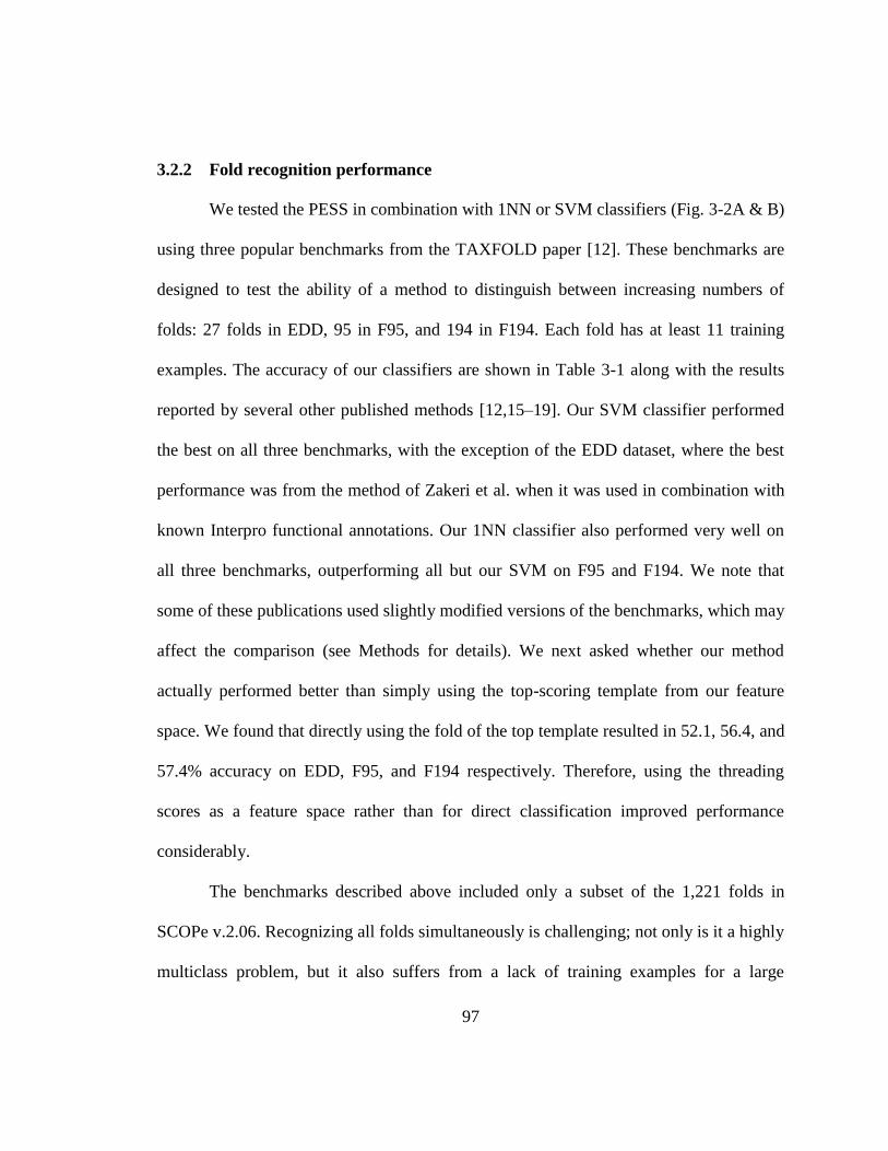
97
3.2.2 Fold recognition performance
We tested the PESS in combination with 1NN or SVM classifiers (Fig. 3-2A & B)
using three popular benchmarks from the TAXFOLD paper [12]. These benchmarks are
designed to test the ability of a method to distinguish between increasing numbers of
folds: 27 folds in EDD, 95 in F95, and 194 in F194. Each fold has at least 11 training
examples. The accuracy of our classifiers are shown in Table 3-1 along with the results
reported by several other published methods [12,15–19]. Our SVM classifier performed
the best on all three benchmarks, with the exception of the EDD dataset, where the best
performance was from the method of Zakeri et al. when it was used in combination with
known Interpro functional annotations. Our 1NN classifier also performed very well on
all three benchmarks, outperforming all but our SVM on F95 and F194. We note that
some of these publications used slightly modified versions of the benchmarks, which may
affect the comparison (see Methods for details). We next asked whether our method
actually performed better than simply using the top-scoring template from our feature
space. We found that directly using the fold of the top template resulted in 52.1, 56.4, and
57.4% accuracy on EDD, F95, and F194 respectively. Therefore, using the threading
scores as a feature space rather than for direct classification improved performance
considerably.
The benchmarks described above included only a subset of the 1,221 folds in
SCOPe v.2.06. Recognizing all folds simultaneously is challenging; not only is it a highly
multiclass problem, but it also suffers from a lack of training examples for a large

98
fraction of the folds. We focused on our 1NN classifier, which requires only a single
training example per fold, to scale to the full fold recognition task. To train the classifier
to recognize all folds, we downloaded domain sequences from the Astral database [2]
corresponding to SCOPe (v.2.06) filtered to less than 20% pairwise identity, which we
call SCOP-20. This dataset contains 7,659 sequences covering all 1,221 folds in classes
“a” through “g”. The same 1,814 templates were used to extract features, as before. To
create a separate test set, we also downloaded the SCOPe sequences filtered to 40%
identity and then removed any overlap between this set and the SCOP-20 set. This
resulted in 6,322 sequences in 609 folds, which we call the SCOP-40 dataset. Using 1NN
classification, 97.6% of SCOP-40 domains were classified into the correct fold
(precision=0.964, recall=0.95). Using a combined SVM+1NN classifier (see Methods)
did not improve performance (acc=96.9%, precision=0.917, recall=0.938), indicating that
the 1NN classifier alone is sufficient for good classification on this dataset. To create a
more difficult test, we filtered the SCOP-40 set so all test examples had less than 25%
identity with a training example. The classification performance remained strong
(acc=96.2%, precision=0.947, recall=0.922). Finally, to rule out any biasing effect of
redundancy between test examples and the 1,814 feature templates, we removed any
SCOP-40 examples that had more than 25% identity with one of the templates (896
examples). This had virtually no effect on the classification (acc=97.6%,
precision=0.956, recall=0.951).
Of the folds represented in the SCOP-20 training set, 86.5% (1,055) have fewer
than 10 training examples, and almost half (605) are “orphan” folds with only one
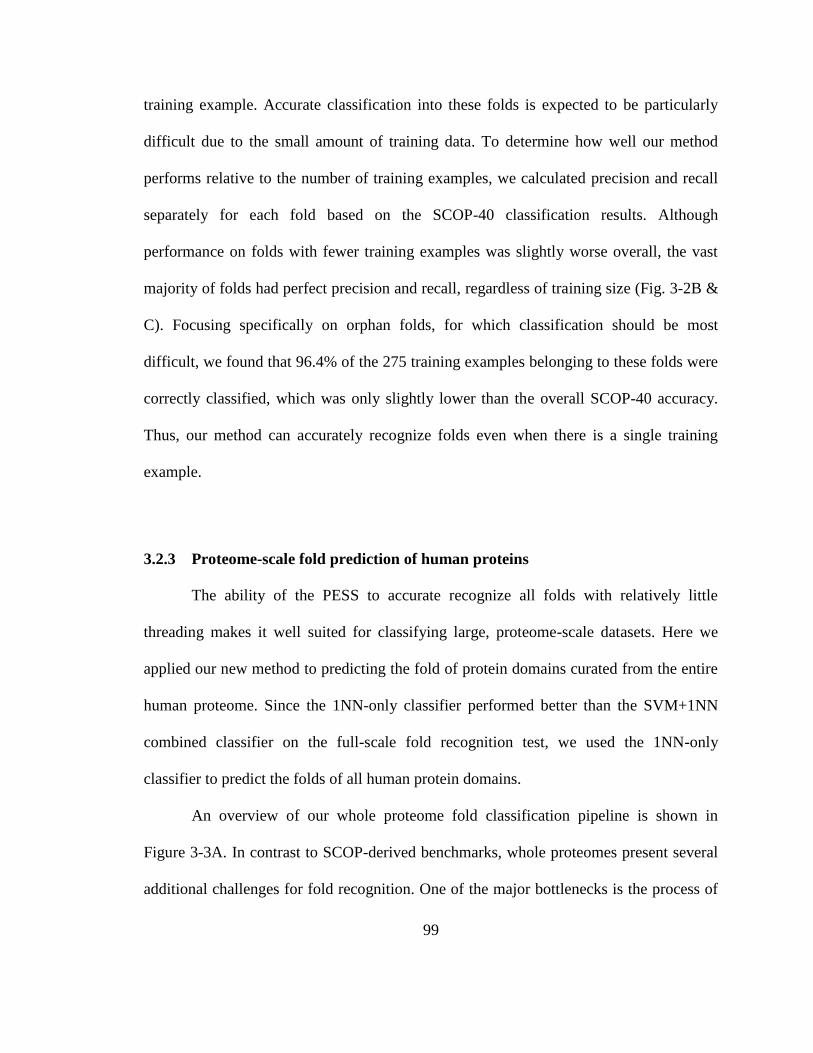
99
training example. Accurate classification into these folds is expected to be particularly
difficult due to the small amount of training data. To determine how well our method
performs relative to the number of training examples, we calculated precision and recall
separately for each fold based on the SCOP-40 classification results. Although
performance on folds with fewer training examples was slightly worse overall, the vast
majority of folds had perfect precision and recall, regardless of training size (Fig. 3-2B &
C). Focusing specifically on orphan folds, for which classification should be most
difficult, we found that 96.4% of the 275 training examples belonging to these folds were
correctly classified, which was only slightly lower than the overall SCOP-40 accuracy.
Thus, our method can accurately recognize folds even when there is a single training
example.
3.2.3 Proteome-scale fold prediction of human proteins
The ability of the PESS to accurate recognize all folds with relatively little
threading makes it well suited for classifying large, proteome-scale datasets. Here we
applied our new method to predicting the fold of protein domains curated from the entire
human proteome. Since the 1NN-only classifier performed better than the SVM+1NN
combined classifier on the full-scale fold recognition test, we used the 1NN-only
classifier to predict the folds of all human protein domains.
An overview of our whole proteome fold classification pipeline is shown in
Figure 3-3A. In contrast to SCOP-derived benchmarks, whole proteomes present several
additional challenges for fold recognition. One of the major bottlenecks is the process of

100
segmenting whole proteins into domains, which is often slow and error-prone. We did not
attempt to address this issue here, but instead make use of the existing domain
segmentation of the human proteome performed by the Proteome Folding Project [5].
Another challenge is recognizing domains that do not belong in any of the known fold
categories, e.g. due to segmentation errors, being disordered, or belonging to a previously
undiscovered fold. To address this problem, we defined a distance threshold for
classification based on the typical distance between a domain and its nearest neighbor
when the true fold of the domain is not represented in the feature space (see Methods).
When a query domain’s nearest neighbor is farther than this threshold distance, the
domain is assigned to a “no classification” category (Fig. 3-3A).
There were a total of 34,330 human domains with length greater than 30 residues
in the Proteome Folding Project dataset, corresponding to 15,619 proteins. Of these,
20,340 domains (59%) had a nearest neighbor within the distance threshold and were
classified into an existing fold by our method. Only 128 of these domains were
previously placed into a fold with high confidence by the Proteome Folding Project [5].
To test how well our predictions match with what is currently known about human
protein structures, we used a blastp search against PDB to identify 2,211 human domain
sequences with a “known” fold; that is, an identical or highly similar PDB entry with a
SCOPe fold classification. Our classifier made a fold prediction for 1,873 (84.7%) of
these domains, and 95.6% of these predictions exactly matched the known SCOPe fold.
Overall, 757 of the 1,221 SCOPe folds had at least one human domain predicted
by our method. The distribution of domains across folds was highly skewed, with the
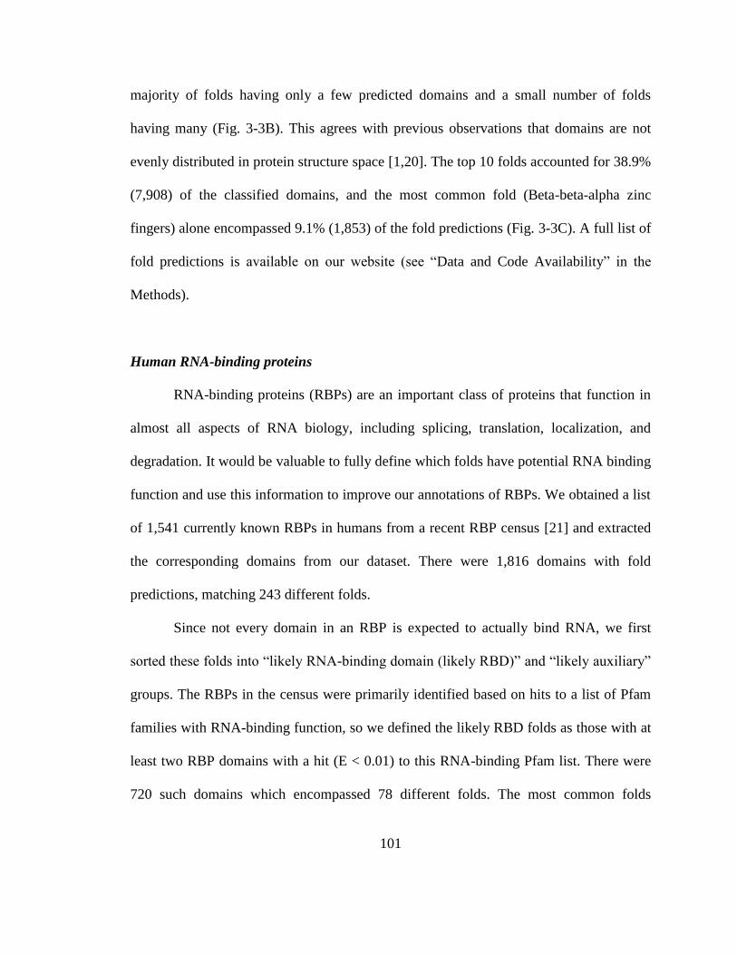
101
majority of folds having only a few predicted domains and a small number of folds
having many (Fig. 3-3B). This agrees with previous observations that domains are not
evenly distributed in protein structure space [1,20]. The top 10 folds accounted for 38.9%
(7,908) of the classified domains, and the most common fold (Beta-beta-alpha zinc
fingers) alone encompassed 9.1% (1,853) of the fold predictions (Fig. 3-3C). A full list of
fold predictions is available on our website (see “Data and Code Availability” in the
Methods).
Human RNA-binding proteins
RNA-binding proteins (RBPs) are an important class of proteins that function in
almost all aspects of RNA biology, including splicing, translation, localization, and
degradation. It would be valuable to fully define which folds have potential RNA binding
function and use this information to improve our annotations of RBPs. We obtained a list
of 1,541 currently known RBPs in humans from a recent RBP census [21] and extracted
the corresponding domains from our dataset. There were 1,816 domains with fold
predictions, matching 243 different folds.
Since not every domain in an RBP is expected to actually bind RNA, we first
sorted these folds into “likely RNA-binding domain (likely RBD)” and “likely auxiliary”
groups. The RBPs in the census were primarily identified based on hits to a list of Pfam
families with RNA-binding function, so we defined the likely RBD folds as those with at
least two RBP domains with a hit (E < 0.01) to this RNA-binding Pfam list. There were
720 such domains which encompassed 78 different folds. The most common folds
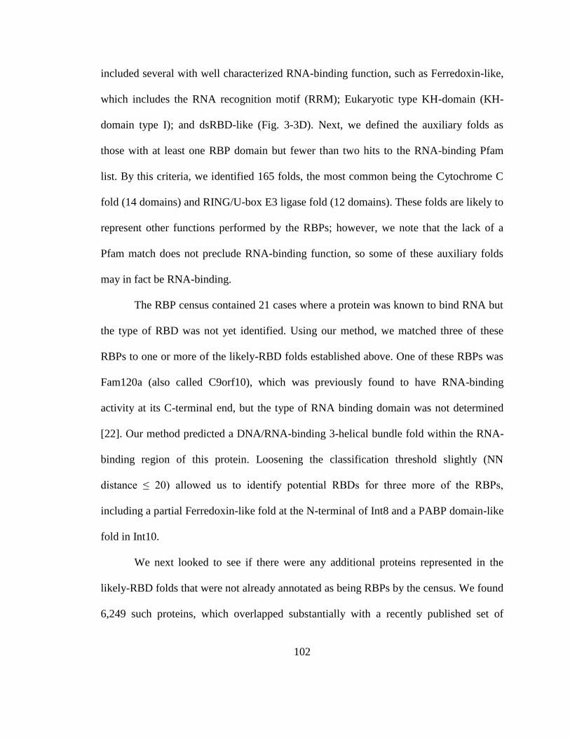
102
included several with well characterized RNA-binding function, such as Ferredoxin-like,
which includes the RNA recognition motif (RRM); Eukaryotic type KH-domain (KH-
domain type I); and dsRBD-like (Fig. 3-3D). Next, we defined the auxiliary folds as
those with at least one RBP domain but fewer than two hits to the RNA-binding Pfam
list. By this criteria, we identified 165 folds, the most common being the Cytochrome C
fold (14 domains) and RING/U-box E3 ligase fold (12 domains). These folds are likely to
represent other functions performed by the RBPs; however, we note that the lack of a
Pfam match does not preclude RNA-binding function, so some of these auxiliary folds
may in fact be RNA-binding.
The RBP census contained 21 cases where a protein was known to bind RNA but
the type of RBD was not yet identified. Using our method, we matched three of these
RBPs to one or more of the likely-RBD folds established above. One of these RBPs was
Fam120a (also called C9orf10), which was previously found to have RNA-binding
activity at its C-terminal end, but the type of RNA binding domain was not determined
[22]. Our method predicted a DNA/RNA-binding 3-helical bundle fold within the RNA-
binding region of this protein. Loosening the classification threshold slightly (NN
distance ≤ 20) allowed us to identify potential RBDs for three more of the RBPs,
including a partial Ferredoxin-like fold at the N-terminal of Int8 and a PABP domain-like
fold in Int10.
We next looked to see if there were any additional proteins represented in the
likely-RBD folds that were not already annotated as being RBPs by the census. We found
6,249 such proteins, which overlapped substantially with a recently published set of
103
6,657 novel RBP predictions by RBPPred (1,981 overlapping genes not previously
annotated as RBPs)[23]. The ~2,000 concordant predictions by these two orthogonal
methods more than double the number of previous RBP annotations [21]. We note that
for many of our RBP predictions, we cannot confidently predict their RBP status based
on fold alone because some of the likely-RBD folds have other functions besides RNA-
binding (e.g. some superfamilies of the Ferredoxin-like fold can be protein binding
instead of RNA binding), which may explain some of the non-overlapping predictions
between our method and RBPPred. Nonetheless, several of the likely-RBD folds appear
to be highly enriched in known RNA-binding domains, suggesting that functional
annotation transfer is possible for these folds. For example, of the 32 domains predicted
by our method to have the KH-domain fold, only four did not have a hit to the RNA-
binding Pfam list, and of these, three were already known to be KH-domain RBPs based
on the RBP census. The one domain that was not in the census was part of the Blom7
protein (also called KIAA0907), which has an experimentally determined structure
(PDB: 2YQR) that confirms structural similarity to the KH-domain, despite the lack of a
Pfam match. A full list of our new RBP predictions and likely-RBD folds is available on
our website (see “Data and Code Availability” in the Methods).
Novel folds in the human proteome
Each year at least a few new folds are added to SCOPe (e.g. 13 new folds were
added in the latest release). As noted above, there were ~14,000 human protein domains,
or ~40% of domains, that were not assigned to known folds. While some of these might
104
be due to problems of segmentation, we hypothesize many of them represent
uncharacterized folds. As a preliminary analysis of potential novel folds in the human
proteome, we extracted a set of human domains that were not close to any of our training
examples (NN distance ≥ 30) and clustered them (Methods). This resulted in 36 clusters
(Fig. 3-4A), which we examined for evidence of novel folds.
We first looked for incorrect domain boundary prediction or errors of our
prediction method. Many of the domains were unusually long (>500 residues) compared
to the average domain in the training set (195 residues), suggesting that they may in fact
be multiple domains. For example, there were four neighboring clusters that contained
almost exclusively domains from the Cadherin family of proteins. Most of these domains
were longer than 500 residues and overlapped multiple repeats of the Cadherin motif
based on Pfam annotations. The Cadherin fold is modeled as a single repeat in SCOPe, so
this is likely a case where fold classification failed due to improper domain definition. A
similar problem was observed for six clusters containing domains from several different
classes of ATP/GTP binding proteins, where each domain spanned multiple distinct Pfam
annotations that are likely to represent separate folds. Overall, we found that 26 of the
clusters were potentially the result of such segmentation errors.
The largest cluster contained 208 domains, most of which were of a reasonable
length (289 residues on average). On closer examination, we found that a large fraction of
these domains were predicted to have a coiled coil structure. The SCOPe hierarchy places
most coiled coil domains in a separate class (class H) that was not included in the training
data. Therefore, this cluster can possibly be explained by the absence of the correct fold

105
within our training data, although it is not truly novel. Eight other neighboring clusters
were also found to have predominantly coiled coil structure, indicating that these
structures can potentially explain a substantial fraction of our unclassified domains.
We also examined the un-clustered domains, which might be isolated examples of
novel folds. One domain, the fourth predicted domain of the protein Limbin (residues
775-1067), was found not to overlap any known Pfam, SCOP, or other structural
annotation. Although this domain was located in the feature space in proximity to the
coiled coil clusters (Fig. 3-4A), it is predicted to be only partially coiled coil (Fig. 3-4B).
We performed a more thorough template search for this domain using HHPred [24],
RaptorX [25], and SPARKS-X [26] webservers, but did not identify a significant
template match. We therefore used the Robetta webserver [27] to create an de novo
model for this domain, which shows a mostly alpha helix structure (Fig. 3-4C). Limbin is
the protein product of the gene EVC2, which is involved in the hedgehog signaling
pathway and is frequently mutated in Ellis-van Creveld syndrome [28,29]. Interestingly,
one of the mutations linked to this disease is found within our domain of interest
(Arg870Trp; rs137852928) [28], suggesting that this region is functionally important.
Whether this region represents a truly new fold will require additional analysis, but
overall these results support the idea that the PESS can be used to identify novel structure
groups.

106
3.2.4 Finding missing hedgehog proteins in C. elegans
The Hedgehog (Hh) signaling pathway plays an essential role in embryo
development, cell proliferation, and tissue patterning in vertebrates and many
invertebrates, including Drosophila [30]. Although many Hh-related genes have
homologs in C. elegans, several key components of the pathway appear to be missing,
including Smoothened (smo), Fused (fu), Suppressor of fused (Su(fu)), Cos2 (cos), and
Hh itself. We asked whether we might be able to identify distant homologs to these
missing genes using structural similarity search with the PESS.
To perform a proteome-scale structural similarity search, we first obtained all
proteins in the C. elegans proteome, split them into domains, and mapped them to the
PESS (see Methods). Next we obtained the sequences of the missing Hh-related genes
from Drosophila, manually split them into their known functional domains, and mapped
these to PESS as well. For each Hh-related protein, we used its domains as “queries” to
obtain the closest 500 C. elegans domains within the PESS, which should represent the
most structurally similar sequences in the C. elegans proteome. We then filtered the
domain lists for each query protein to identify any C. elegans proteins that appeared on
all (or most) of the lists—that is, proteins that have structural similarity to all (or most) of
the domains of the query.
The closest matches for each of the Hh-related proteins are shown in Table 3-2. We
found at least one potential structural match for each of the five query proteins. There are
several promising results; for example, several serpentine receptors were found for
Smoothened that also have similarity to its N-terminal domain, and several kinesin-like

107
proteins were found for Cos2 that also have distant similarity to its interaction domains.
More work will be needed to verify whether these proteins function in the Hh pathway.
These results demonstrate an alternative use of the PESS as a direct method for structural
querying of whole proteomes, independent of the framework of SCOPe folds used for
classification in the previous sections.
3.3 Discussion
Here we have demonstrated the utility of an empirically derived structural feature
space composed of threading scores (the PESS) for addressing the problem of fold
recognition. The most important characteristics of such a multi-dimensional feature space
are the ability to combine characteristics of multiple fold templates for fold recognition
and the ability to potentially identify entirely novel folds through interpolation of the
feature space. Many types of classifiers can be used in conjunction with this feature
space; we showed here that linear SVM achieved good performance on benchmarks
where at least 10 training examples were available per fold, and 1NN worked well in the
more general case to recognize all known folds. We applied our method to the human
proteome, predicted high confidence fold classifications for 20,340 domains, and showed
that these predictions can be used to make functional inferences as illustrated by the class
of RNA-binding proteins. A distinct advantage of the PESS is that it only requires a
single training example per fold when used in conjunction with a 1NN classifier,
allowing us to make predictions for all currently known folds in SCOPe. This is critical,
since almost half of all SCOPe folds have only one training example in SCOP-20.
108
Another advantage of the 1NN classifier is that adding new training data does not require
re-training the whole classifier, making it simple to update the model as new data become
available.
One of the limitations of methods that rely on threading is the large amount of
time the threading process takes. Threading against all PDB templates can take hours or
even days per domain, depending on the computational resources available. In our
method, we save time by only threading against representative templates. Nonetheless,
threading is still the major time bottleneck, with a single average-sized (200 residue)
domain taking 26 ± 2.5 minutes to thread against the 1,814 templates on one CPU core.
To make this more feasible for genome-sized datasets, which typically have thousands or
tens of thousands of domains, we have implemented an option for parallel processing of
the input sequences. Another possible way to decrease the threading time would be to
reduce the number of templates in our library. Preliminary results indicate that,
depending on the classifier used, the feature space can be substantially reduced with only
a minor impact on classification accuracy. In fact, given our framework, we hypothesize
that we can create feature spaces at different scales such that threading can be applied in a
hierarchical sequence.
The relationship between the structure of macromolecules to their function is a
key annotation principle for computational inference. As the number of solved examples
increase, we hypothesize that data-driven feature extraction coupled with machine
learning methods as in our method and also in methods like deep learning [31], will have
high utility in extending whole genome/proteome annotations.
109
3.4 Methods
Feature extraction and classification
Features were created for each input sequence by threading the sequence against a
library of 1,814 structure templates to produce a vector of 1,814 threading scores. These
scores represent the compatibility of the sequence with each template structure. Each
score is directly used as a numerical coordinate within the feature space, which we call
the Protein Empirical Structure Space (PESS). Threading was done using CNFalign_lite
from the RaptorX package v.1.62 [32,33]. This program outputs a raw threading score for
each query-template pair that is calculated from the optimal alignment of the query
sequence and the template [32,33]. The template library was the default library provided
by RaptorX. These 1,814 templates represent a wide range of different structures with
low redundancy, but do not necessarily represent all known folds.
Training sequences were threaded against the templates and the resulting scores
were normalized by z-standardization. Test sequences were threaded and normalized
using the normalization parameters derived from the training sequences.
We constructed fold predictors over the PESS using both a first Nearest Neighbor
(1NN) classifier and Support Vector Machine (SVM) classifier. For the 1NN classifier,
pairwise Euclidean distances between each training and testing sequence were calculated,
and each test sequence was classified into a fold by finding the closest training neighbor
and transferring its fold label to the test sequence. For the support vector machine (SVM)

110
classifier, a linear SVM was trained using the one-vs-all multiclass approach with the C
parameter (which controls the penalization of misclassification during training) set to
1/N, where N is the number of positive examples in a given fold.
We also constructed a joint SVM+1NN classifier to assist in identification of fold
classes with very small number of training examples. First, a linear SVM was trained as
described above to recognize only folds that had at least 20 training examples (“large
folds”). The remaining sequences in the training set (“small folds”) were combined into a
single class labeled “other”, and this class was not used for classification. A separate
1NN classifier was trained on only the small fold training examples. Classification was
then done in two phases: first, all test examples were provided to the SVM, and any test
example that received a positive confidence score (based on the signed distance from the
hyperplane) was classified into whichever fold gave the highest confidence score; second,
the examples that were not classified in the first step were passed to the 1NN model for
classification.
All classifiers were implemented in Python using the scikit-learn package [34].
Performance assessment
Prediction accuracy was calculated as the fraction of test examples that were
classified into the correct fold. Precision (the number of true positives divided by the sum
of the true and false positives) and recall (the number of true positive divided by the sum
of the true positives and false negatives) were calculated separately for each fold and
averaged across the folds. For both precision and recall, we excluded folds where the
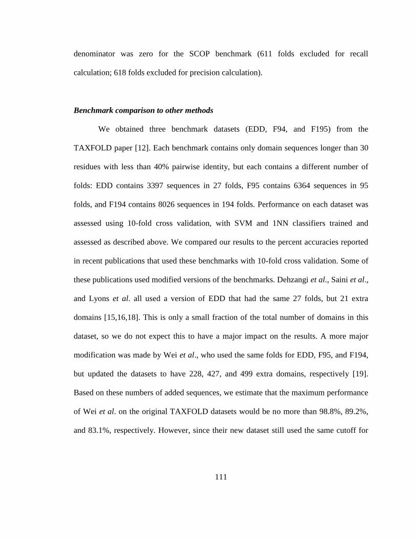
111
denominator was zero for the SCOP benchmark (611 folds excluded for recall
calculation; 618 folds excluded for precision calculation).
Benchmark comparison to other methods
We obtained three benchmark datasets (EDD, F94, and F195) from the
TAXFOLD paper [12]. Each benchmark contains only domain sequences longer than 30
residues with less than 40% pairwise identity, but each contains a different number of
folds: EDD contains 3397 sequences in 27 folds, F95 contains 6364 sequences in 95
folds, and F194 contains 8026 sequences in 194 folds. Performance on each dataset was
assessed using 10-fold cross validation, with SVM and 1NN classifiers trained and
assessed as described above. We compared our results to the percent accuracies reported
in recent publications that used these benchmarks with 10-fold cross validation. Some of
these publications used modified versions of the benchmarks. Dehzangi et al., Saini et al.,
and Lyons et al. all used a version of EDD that had the same 27 folds, but 21 extra
domains [15,16,18]. This is only a small fraction of the total number of domains in this
dataset, so we do not expect this to have a major impact on the results. A more major
modification was made by Wei et al., who used the same folds for EDD, F95, and F194,
but updated the datasets to have 228, 427, and 499 extra domains, respectively [19].
Based on these numbers of added sequences, we estimate that the maximum performance
of Wei et al. on the original TAXFOLD datasets would be no more than 98.8%, 89.2%,
and 83.1%, respectively. However, since their new dataset still used the same cutoff for
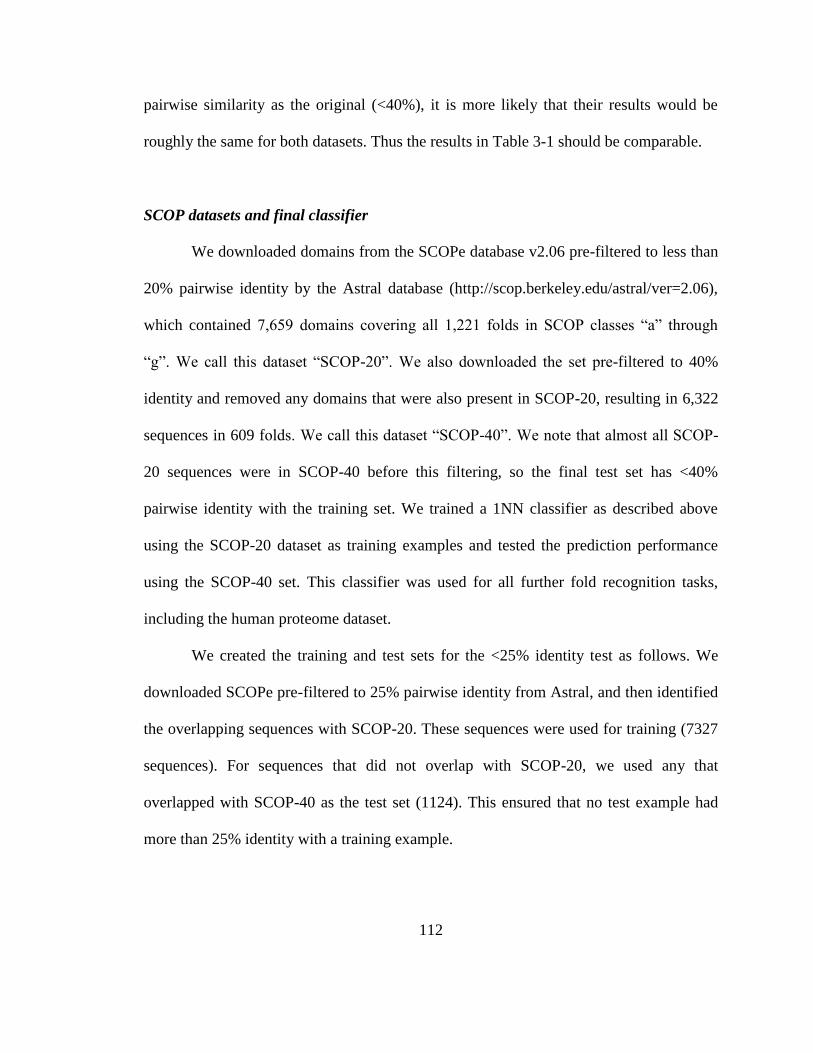
112
pairwise similarity as the original (<40%), it is more likely that their results would be
roughly the same for both datasets. Thus the results in Table 3-1 should be comparable.
SCOP datasets and final classifier
We downloaded domains from the SCOPe database v2.06 pre-filtered to less than
20% pairwise identity by the Astral database (http://scop.berkeley.edu/astral/ver=2.06),
which contained 7,659 domains covering all 1,221 folds in SCOP classes “a” through
“g”. We call this dataset “SCOP-20”. We also downloaded the set pre-filtered to 40%
identity and removed any domains that were also present in SCOP-20, resulting in 6,322
sequences in 609 folds. We call this dataset “SCOP-40”. We note that almost all SCOP-
20 sequences were in SCOP-40 before this filtering, so the final test set has <40%
pairwise identity with the training set. We trained a 1NN classifier as described above
using the SCOP-20 dataset as training examples and tested the prediction performance
using the SCOP-40 set. This classifier was used for all further fold recognition tasks,
including the human proteome dataset.
We created the training and test sets for the <25% identity test as follows. We
downloaded SCOPe pre-filtered to 25% pairwise identity from Astral, and then identified
the overlapping sequences with SCOP-20. These sequences were used for training (7327
sequences). For sequences that did not overlap with SCOP-20, we used any that
overlapped with SCOP-40 as the test set (1124). This ensured that no test example had
more than 25% identity with a training example.

113
To remove redundancy between the SCOP-40 test examples and the 1,814 feature
templates, we first obtained the original sequences used to generate the templates, which
is included in the template file. We then performed a blastp search of the template
sequences using all the SCOP-40 sequences as queries, and removed any SCOP-40
examples that had more than 25% identity over at least 90% of their length with one of
the template sequences.
Human protein analysis
Protein domain sequences for 94 species from the Proteome Folding Project [5]
were downloaded from the Yeast Resource Center public data repository
(http://www.yeastrc.org/pdr/pages/download.jsp). To obtain only human sequences, we
filtered for protein identifiers marked as “NCBI NR” and had “[Homo sapiens]” in the
description. There were a total of 34,330 human domains with length greater than 30
residues, corresponding to 15,619 human proteins.
We classified the domains using the SCOP-20-trained 1NN model with an
additional distance threshold to filter out domains that do not belong in any of the
represented folds. We determined the threshold nearest-neighbor distance for
classification as follows: for each test sequence in SCOP-40, we calculated the nearest
neighbor distance before and after removing all SCOP-20 training sequences that
belonged to the same fold as the test sequence. We found that a distance threshold of 17.5
provided a good balance between false positives and false negatives (FPR = 9.27%, FNR

114
= 9.49%). After classification with 1NN, only the domains with a nearest-neighbor
distance below this threshold we considered confident fold predictions.
Human domain sequences were mapped to PDB entries using a blastp search of
PDB requiring that at least 75% of the sequence length had at least 90% identity with a
PDB sequence to consider it a match. PDB matches were then mapped to SCOPe
classifications using the dir.cla.scope.txt (v.2.06) annotation file downloaded from the
SCOPe website.
RNA-binding proteins
A list of 1,541 known human RBPs was obtained from a recent review [21]. Gene
names of the RBPs were matched up to the human protein GIs using the UniProt ID
mapping tool, and 1,093 of the RBPs were matched to one or more domains (3,263
domains total). This review also defined a list of 799 Pfam domains with functions
related to RNA binding, which we used to filter the 3,263 RBP domains down to those
that were most likely to be RNA-binding. Domains were assigned PfamA annotations
using hmmscan (http://hmmer.org/). Both a “full-sequence” E ≤ 0.01 and a “best 1” E ≤
0.1 was required for assignment. We compared our novel RBP predictions with the novel
predictions from the RBPPred paper [23] on the gene level by mapping UniProt IDs to
gene names for each list using the ID conversion tool on the UniProt website. Not all
UniProt IDs could be mapped to a gene name. The final unique gene lists contained 6,589
genes for RBPPred and 5,668 genes for our method, which we used to compute the
overlap.

115
Novel folds
We extracted all human domains with a nearest neighbor distance ≥30 and
performed t-SNE on the PESS projections of these domains using scikit-learn with
parameters “perplexity = 10, init = ‘pca’, random_state=123”. Domains were then
clustered using DBSCAN from scikit-learn with parameters “eps = 5, min_samples = 5”.
Domains and clusters were manually examined for potential boundary prediction errors
or previous structural annotations.
C. elegans Hedgehog gene analysis
We downloaded the canonical protein sequences for the Caenorhabditis elegans
proteome from UniProt. Each protein was split into domains based on DomainFinder
Gene3D predictions [[REF]]. If there were regions between, before, or after predicted
domains that were longer than 30 aa but did not have a Gene3D prediction, we also
included those. If a “filled in” region such as this was longer than 450 aa, we used a
sliding window of 300 aa (slide = 150 aa) to break it into smaller pieces. The fold of each
domain was predicted using the methods described above. Known Hh-related protein
sequences from Drosophila melanogaster were downloaded from UniProt, manually split
into domains based on literature annotations of functional domains, and mapped to the
PESS as above.
Data and Code Availability

116
Benchmark datasets, training data, and all human fold and RBP predictions are
available at http://kim.bio.upenn.edu/software/pess.shtml. The fold classification source
code is freely available at the same website or at https://github.com/sarahmid/PESS.
Author Contributions
S.A.M. and J.K. conceived the study and wrote the manuscript. S.A.M.
implemented the feature space and classifier, applied it to the human proteome, and
interpreted results. J.I. contributed to classifier development and validation.

117
Figure 3-1. Overview of PESS construction.
Training sequences of known fold are threaded against a set of structure templates, and
the resulting threading scores act as coordinates within a structural feature space (the
PESS). A classifier can then be trained to recognize the subspace occupied by each fold
in the PESS. Different colors indicate the fold of each sequence and are shown here only
for visualization.
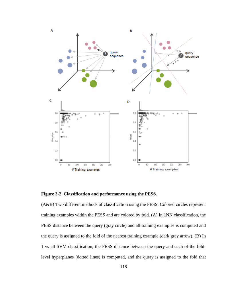
118
Figure 3-2. Classification and performance using the PESS.
(A&B) Two different methods of classification using the PESS. Colored circles represent
training examples within the PESS and are colored by fold. (A) In 1NN classification, the
PESS distance between the query (gray circle) and all training examples is computed and
the query is assigned to the fold of the nearest training example (dark gray arrow). (B) In
1-vs-all SVM classification, the PESS distance between the query and each of the fold-
level hyperplanes (dotted lines) is computed, and the query is assigned to the fold that
119
gives the best score (dark gray arrow), based on signed distance from the fold’s
hyperplane. (C) Precision and (D) recall measures were computed for each fold
separately after 1NN classification using the PESS and plotted against the number of
training examples for each fold. Marginal histograms show the distribution of folds along
each axis.

120
Figure 3-3. Fold classification of the human proteome.
(A) Overview of classification process. Full length human protein sequences were split at
predicted domain boundaries to create one or more separate domain sequences per
protein (Drew et al. 2011). Domain sequences were mapped to the PESS and classified
by 1NN classification. A threshold was applied to the nearest neighbor distance (dotted
circle), whereby only domains with a nearest neighbor closer than the threshold distance
were classified. (B) PCA projection of fold centroids within the PESS, scaled by number

121
of human domains predicted to belong to that fold. Centroids were calculated based on
the location of each fold’s training examples within the PESS and are colored by SCOP
class. (C) Top ten folds by number of human domain predictions. (D) Top ten likely
RNA-binding folds, ranked by number of confirmed RNA-binding domains (RBDs).
Confirmed RBDs were determined based on matches to a curated list of RNA-binding
related Pfam families.
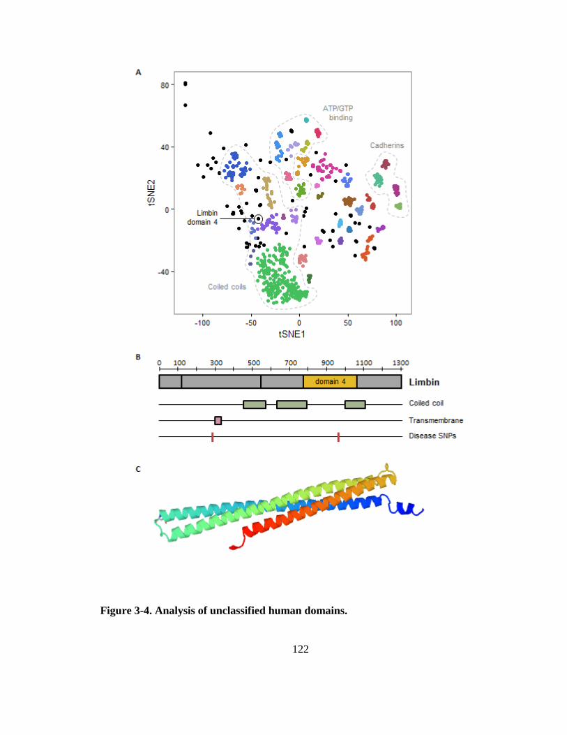
122
Figure 3-4. Analysis of unclassified human domains.
123
(A) t-SNE projection of human domains with nearest-neighbor distance ≥ 30. Colors
indicate cluster assignment by DBSCAN; unclustered domains are shown in black.
Dotted lines show related groups of domains. (B) Overview of the EVC2 protein product,
Limbin, and its known structure elements. The location of the domain with a putative
novel fold is shown in yellow. (C) De novo structure model for part of the Limbin
domain 4 creating using Robetta.

124
Table 3-1. Overall % accuracy on three benchmarks using 10-fold cross validation.
Method EDD F95 F194
Dehzangi et al.a 88.2 - -
Saini et al.a 86.6 - -
Lyons et al.a 93.8 - -
Zakeri et al. 88.8 / 96.9b
- -
Yang and Chen 90.0 82.4 79.6
Wei et al.c 92.6 83.6 78.2
This method – 1NN 90.6 84.6 82.5
This method - SVM 95.7 91.9 90.5 a Using a slightly modified EDD set with 21 additional domains (3418 total) (see Methods)
b With Interpro functional annotations
c Using modified versions of EDD (3625 domains), F95 (6791 domains), and F194 (8525) (see Methods)

125
Table 3-2. Putative structural matches to missing C. elegans Hh-related genes.
Protein Domains required to match Closest C. elegans matches
Hedgehog N-terminal domain (hedge),
C-terminal domain (hog)
trpp-8, CELE_T28F3.5, fbxa-142, spt-5,
tns-1, C41A3.1, lin-18, nmr-1,
CELE_T21C9.6, CELE_F54B3.1, prx-1,
sup-17, mtm-6, CELE_F46G10.2,
C05D12.3, eef-2, CELE_F57C7.4
Smoothened
N-terminal domain,
Frizzled domain,
GPCR-like domain
npr-30, srh-173, srw-139, tyra-3, srw-48,
srw-124, fshr-1
Fused
Kinase domain,
Central domain,
Leucine-rich-repeat domain
chs-2
Suppressor
of fused
Suppressor of fused-like,
Suppressor of fused C-terminal
C41A3.1, plc-1, cec-9, CELE_F27C8.2,
aph-2, age-1, CELE_T23E1.1,
CELE_F59H6.5, glf-1, CELE_T08A11.1,
ddo-3, gcy-25, rde-1, ntp-1, B0511.12,
F52H2.6, CELE_Y61A9LA.10, let-19,
drsh-1, ZK1067.4, CELE_W03A5.1,
CELE_Y16E11A.2, CELE_F22E5.6,
CELE_Y43F8B.19, CELE_Y7A5A.1,
CELE_T05H10.1
Cos2
Kinesin-like domain,
fu-binding domain,
smo-binding domain
unc-116, klp-18, klp-20, zen-4, klp-12,
arc-1

126
3.5 References
1 Koonin, E. V et al. (2002) The structure of the protein universe and genome
evolution. Nature 420, 218–223
2 Fox, N.K. et al. (2014) SCOPe: Structural Classification of Proteins—extended,
integrating SCOP and ASTRAL data and classification of new structures. Nucleic
Acids Res. 42, D304–D309
3 Kim, S.H. et al. (2005) Structural genomics of minimal organisms and protein fold
space. J. Struct. Funct. Genomics 6, 63–70
4 Malmström, L. et al. (2007) Superfamily assignments for the yeast proteome
through integration of structure prediction with the gene ontology. PLoS Biol. 5,
758–768
5 Drew, K. et al. (2011) The Proteome Folding Project: Proteome-scale prediction of
structure and function. Genome Res. 21, 1981–1994
6 Hildebrand, A. et al. (2009) Fast and accurate automatic structure prediction with
HHpred. Proteins Struct. Funct. Bioinforma. 77, 128–132
7 Huang, Y.J. et al. (2014) Assessment of template-based protein structure
predictions in CASP10. Proteins Struct. Funct. Bioinforma. 82, 43–56
8 Roy, A. et al. (2010) I-TASSER: a unified platform for automated protein
structure and function prediction. Nat. Protoc. 5, 725–38
9 Cheng, J. and Baldi, P. (2006) A machine learning information retrieval approach
to protein fold recognition. Bioinformatics 22, 1456–1463
10 Jo, T. et al. (2015) Improving Protein Fold Recognition by Deep Learning
Networks. Sci. Rep. 5, 17573
11 Dubchak, I. et al. (1999) Recognition of a protein fold in the context of the SCOP
classification. Proteins Struct. Funct. Genet. 35, 401–407
12 Yang, J.-Y. and Chen, X. (2011) Improving taxonomy-based protein fold
recognition by using global and local features. Proteins 79, 2053–64
13 Scholkopf, B. and Mika, S. (1999) Input space versus feature space in kernel-based
methods. IEEE Trans. Neural Netw. 10, 1000–1017
14 Middleton, S.A. and Kim, J. (2014) NoFold: RNA structure clustering without
127
folding or alignment. RNA 20, 1671–1683
15 Dehzangi, A. et al. (2014) A segmentation-based method to extract structural and
evolutionary features for protein fold recognition. IEEE/ACM Trans. Comput.
Biol. Bioinforma. 11, 510–519
16 Saini, H. et al. (2015) Probabilistic expression of spatially varied amino acid
dimers into general form of Chou׳s pseudo amino acid composition for protein fold
recognition. J. Theor. Biol. 380, 291–298
17 Zakeri, P. et al. (2014) Protein fold recognition using geometric kernel data fusion.
Bioinformatics 30, 1850–1857
18 Lyons, J. et al. (2015) Advancing the Accuracy of Protein Fold Recognition by
Utilizing Profiles from Hidden Markov Models. IEEE Trans. Nanobioscience 14,
761–772
19 Wei, L. et al. (2015) Enhanced Protein Fold Prediction Method Through a Novel
Feature Extraction Technique. IEEE Trans. Nanobioscience 14, 649–659
20 Orengo, C.A. et al. (1994) Protein superfamilles and domain superfolds. Nature
372, 631–634
21 Gerstberger, S. et al. (2014) A census of human RNA-binding proteins. Nat. Rev.
Genet. 15, 829–845
22 Tanaka, M. et al. (2009) A novel RNA-binding protein, Ossa/C9orf10, regulates
activity of Src kinases to protect cells from oxidative stress-induced apoptosis.
Mol. Cell. Biol. 29, 402–413
23 Zhang, X. and Liu, S. (2017) RBPPred: predicting RNA-binding proteins from
sequence using SVM. Bioinformatics btw730,
24 Soding, J. et al. (2005) The HHpred interactive server for protein homology
detection and structure prediction. Nucleic Acids Res. 33, W244–W248
25 Källberg, M. et al. (2012) Template-based protein structure modeling using the
RaptorX web server. Nat. Protoc. 7, 1511–1522
26 Yang, Y. et al. (2011) Improving protein fold recognition and template-based
modeling by employing probabilistic-based matching between predicted one-
dimensional structural properties of query and corresponding native properties of
templates. Bioinformatics 27, 2076–2082
27 Bradley, P. et al. (2005) Toward High-Resolution de Novo Structure Prediction for
Small Proteins. Science (80-. ). 309, 1868–1871

128
28 Galdzicka, M. et al. (2002) A new gene, EVC2, is mutated in Ellis–van Creveld
syndrome. Mol. Genet. Metab. 77, 291–295
29 D’Asdia, M.C. et al. (2013) Novel and recurrent EVC and EVC2 mutations in
Ellis-van Creveld syndrome and Weyers acrofacial dyostosis. Eur. J. Med. Genet.
56, 80–87
30 Varjosalo, M. and Taipale, J. (2008) Hedgehog: Functions and mechanisms. Genes
Dev. 22, 2454–2472
31 LeCun, Y. et al. (2015) Deep learning. Nature 521, 436–444
32 Ma, J. et al. (2012) A conditional neural fields model for protein threading.
Bioinformatics 28, i59–i66
33 Ma, J. et al. (2013) Protein threading using context-specific alignment potential.
Bioinformatics 29, i257-65
34 Pedregosa, F. et al. (2011) Scikit-learn: Machine Learning in Python. J. Mach.
Learn. Res. 12, 2825–2830

129
Chapter 4: Structures and plasticity: analysis of
dendritically targeted RNAs and the “local proteome”
4.1 Introduction
Neurons require local protein synthesis within the dendrites to produce long-lasting
synaptic potentiation [1] (see also section 1.3.3 of this thesis). Importantly, in order for
this local synthesis to occur, mRNAs must first be transported to the dendrites. Although
RNA localization and local translation have been studied for over 20 years, there are still
many aspects of these processes that remain unclear. In this chapter, I will address three
open questions, outlined below, with a particular focus on the under-studied roles of
RNA secondary structure and protein tertiary structure.
Which RNAs are dendritically localized?
Multiple studies have profiled RNAs that are localized to the dendrites using
various methods [2–10]. Despite these efforts, there is still no firm consensus on the set
of dendritically localized RNAs. Most recently, three studies used high-throughput RNA
sequencing (RNA-seq) to identify dendritically-enriched RNAs in rodent neurons. First,

130
Cajigas et al. performed bulk RNA-seq on the neuropil (dendrite-rich) region of rat CA1
hippocampal slices and predicted 2,550 dendritic RNAs [7]. Second, Ainsley et al. used
epitope-tagged ribosomes that were expressed specifically in neurons (but not other brain
cell types) to purify ribosome-bound RNA from mouse CA1 neuropil punches, predicting
1,890 dendritic RNAs [8]. Most recently, Taliaferro et al. used a culture system where
cells were grown on a porous membrane that allows processes to pass through, but not
cell bodies, thus allowing them to collect and sequence processes with relative purity
(similar to [5]) [10]. This allowed them to identify 778 dendritic RNAs (and more with
isoform-specific localization). Although in theory RNA-seq studies such as these should
produce a comprehensive picture of the dendritic transcriptome, each of these studies had
experimental limitations that complicate the interpretation of the results. The Cajigas
study was limited by the presence of non-neuronal and non-dendritic material in the
neuropil, such as glia and interneurons, which make it difficult to pinpoint which RNAs
came from neuronal dendrites. In addition, due to the filtering steps the authors used to
remove suspected contaminating RNAs (including known nuclear-related genes), many
true dendritic RNAs may have been removed. The Ainsley study, which was also
performed with tissue slices, alleviated some of these concerns by increasing the
specificity of the RNA capture for only neuronal dendrites. However, in gaining this
specificity, Ainsley et al. may also have lost some sensitivity, since their method only
captures ribosome-associated RNAs. Finally, the Taliaferro study—while free from
concerns about tissue-related contamination—relied mostly on CAD and N2A cell lines
for their results. Although these cell lines are derived from neurons and grow processes

131
when induced to differentiate, their degree of divergence from primary neurons is
unclear.
Due to these limitations, there is still ambiguity about which RNAs are present in
the dendrites. Studies that are more specific in their capture of dendritic RNA are needed
for primary cells. Although study of dendrites in vivo would be ideal (perhaps using
spatially-precise capture techniques such as that described in [11] or large-scale
fluorescent in situ hybridization (FISH)-based approaches [12–14]), even primary
cultures would give valuable insight. Furthermore, since most studies have used bulk
RNA sequencing of many cells at once, little is known about the variability of dendritic
localization across single neurons. Given the heterogeneity already observed in neuronal
RNA expression on the whole-cell level [15], it would not be surprising if there is
variability of localization. In fact, very early studies have already demonstrated that
individual dendrites of the same neuron can have different transcripts [2]. Further study
of these questions is warranted.
How are RNAs recognized for localization?
If we take the RNA-seq studies described above at face value, then somewhere
between 700 and 2,500 species of RNA are localized to the dendrites. Since the average
neuron is estimated to express between 10,000 and 15,000 genes [11,15], it is clear that
not all RNAs are localized. How then does the neuron perform this large scale sorting of
RNAs that should and should not be dendritically targeted? Most evidence points to the
following model: RNAs that are to be localized contain a cis motif—called a dendritic

132
targeting element (DTE)—which is recognized by a specific RNA binding protein (RBP).
The RBP then mediates association with the transport machinery of the cell and causes
localization [16]. There are probably several different DTEs and localization-mediating
RBPs. However, given that there are currently only ~1,500 known RBPs in humans [17],
of which only a small fraction probably participate in localization, it seems unlikely that
each dendritic RNA is localized by a unique combination of DTE and RBP. Instead,
multiple RNAs probably share the same or very similar DTEs and are transported by the
same RBP. If this is true, then it should be possible to identify DTEs computationally by
looking for sequence elements that are shared among multiple localized RNAs, and
relatively absent in non-localized RNAs. Surprisingly, however, very few DTEs have so
far been found using this method. Most known DTEs were instead identified using trial-
and-error experimental methods, and furthermore seem to be specific to just one or a
small handful of localized RNAs.
Why have DTEs been so elusive thus far? Two possible explanations stand out.
First, most studies have focused exclusively on searching canonical 3’UTRs. Although
this is historically where most localization elements have been found, especially in non-
neuronal contexts, there is growing evidence that other parts of the mRNA could be
involved, such as cytoplasmically retained introns [18]. Recently, a study also identified
over 2,000 previously unannotated distal 3’UTR isoforms, which were conserved
between mouse and human and were mostly specific or upregulated in neuronal tissues
[19]. It is unknown what role these alternative 3’ isoforms play in neurons, but an
exciting possibility is that they contain localization signals. Thus far, these sequences
133
have not been included in the search for DTEs. A second possible explanation for the
lack of known DTEs is that previous studies have not taken secondary structure
sufficiently into account. Many of the known DTEs have an important structural
component or appear to be completely structural in nature, but due to a lack of efficient
algorithms for de novo structural motif discovery, this has not yet been systematically
explored. The combination of a more complete database of localized RNA isoforms with
structure-aware motif finding has great promise for identifying missing localization
signals.
What role do locally translated proteins play in long-term potentiation?
The presumed purpose of localizing so many RNAs to the dendrites—which
requires energy expenditure on the part of the cell—is so that these RNAs can be locally
translated in response to synaptic activation. A corollary of this is that the proteins
produced during local translation (the “local proteome”) should play an important role in
the processes following synaptic activation, particularly those that lead to long-lasting
synaptic plasticity. This is supported by studies showing that inhibiting protein synthesis
in the dendrites blocks late-phase long term potentiation (L-LTP) [1], and has been
shown more specifically to be true for a small handful of individual locally translated
proteins, such as CaMKIIα [20].
So far, however, very little is actually known about the specific role of each
locally translated protein. Gene ontology (GO) analysis can provide a useful overview of
functions enriched in a group, but the annotation is sometimes vague or incomplete for
134
individual proteins and can be susceptible to various biases [21]. As demonstrated in
Chapter 3, protein structure prediction can help fill holes left by other types of annotation
and lead to new functional insights. More specifically, there are several reasons to think
that structure analysis might be particularly useful in the context of understanding the
local proteome. Firstly, the post-synaptic density (PSD) and surrounding dendritic spine
are highly structured formations that depend on a scaffold of interacting proteins for their
function [22–24]. Central to these interactions are protein domains, which usually require
a specific three-dimensional fold in order to function properly. Secondly, mutations
linked to neuropsychiatric diseases have been found to be enriched in synaptic proteins in
human and mouse, and several of these mutations appear to disrupt important structures
[25,26]. A more complete picture of the structures of locally translated proteins will help
both in functional understanding and mutation-impact analysis.
Chapter overview
In this chapter, I use a combination of experimental and computational techniques
to shed new light on the three questions outlined above. To address the first question—
which RNAs are localized to the dendrites?—I dissect individual neurons in primary
culture to obtain somatic and dendritic subcellular compartments with high specificity.
RNA-sequencing then allows for identification of poly-adenylated transcripts in each
compartment. This sequencing is done on the single-cell level to enable direct
comparison of the soma and dendrites from the same original cell, and allows for
assessment of heterogeneity of RNA expression and localization across cells. I use this

135
dataset to identify dendritically enriched RNAs on both the gene and isoform levels,
including the recently identified set of neuron-enriched distal 3’ UTR isoforms [19]. To
address the second question—where are all the common DTEs?—I make use of this
carefully defined set of localized sequences to perform a comprehensive search for RNA
motifs that might be involved in localization. Using the method described in Chapter 2
for de novo identification of RNA structure motifs, I identify several secondary structures
enriched in the localized sequences compared to non-localized background, including
two SINE-derived motifs. Finally, to address the third question—what role do locally
translated proteins play in LTP?—I expand on existing gene-level annotations using
domain-level protein structure information. I use the method described in Chapter 3 to
predict the structural folds of all potential locally-translated proteins (as predicted by the
localization of the RNA) and highlight several new pieces of information the structure
predictions provide, including links to disease. Altogether, these results provide new
insights into RNA localization and locally translated proteins in neurons and demonstrate
the utility of including structure information in functional analysis of macromolecules.
4.2 Results and Discussion
4.2.1 Gene-level localization
To compare the RNAs present in dendrites and somas of individual neurons, we
manually separated the neurites (dendrites/axon) and soma of primary mouse
hippocampal neurons using a micropipette and performed RNA-sequencing on each
subcellular fraction such that we obtained neurite and soma transcriptome of the same

136
cell (Fig. 4-1). We note that the axon is generally small at this culture stage (~5% the
volume of the dendrites) and thus is not expected to make up a large fraction of the
neurite samples. Somas generally contained a wider variety of transcripts than their
corresponding neurites, with an average of 9,206 and 5,827 genes expressed in each
compartment respectively (Fig. 4-2A). As expected, the neurite-expressed genes were
largely a subset of the soma-expressed genes of the same cell (Fig. 4-2B). Genes that
show expression only in the neurites may represent strongly localized RNAs, which we
will investigate further below. All soma and neurite samples expressed housekeeping
genes and neuronal marker genes at high levels, especially pyramidal markers, with little
expression of other brain cell type markers (Fig. 4-3C).
To identify potentially localized RNAs, we used DESeq2 [27] to perform a
differential expression analysis using a paired design, where soma and neurites of the
same original cell were directly compared. DESeq2 reported 3,811 genes significantly
more highly expressed in somas and 387 genes significantly higher in neurites (FDR
corrected p ≤ 0.05) (Fig. 4-3A). Given their relatively higher expression in neurites
compared to soma, these 387 genes are likely to be actively localized, and we therefore
refer to them as localized genes (Table 4-1). Fifty six of these localized genes overlapped
with a curated set of previously annotated dendritic RNAs from tissue and FISH (see
“‘Known dendritic’ gene list” in Methods) (Fig. 4-3B) (p = 4.2e-15; odds ratio = 3.8;
Fisher’s exact test). The localized RNAs were also strongly enriched for GO terms
related to translation and mitochondria, consistent with previous reports [8–10], whereas

137
the somatic RNAs were enriched for functions related to the nucleus, including RNA
splicing and chromatin organization (Fig. 4-3C).
Differential expression analysis identifies genes that have a higher expression in
one condition compared to another. However, in the case of RNA localization, we do not
necessarily expect all localized RNAs to have higher expression in the neurites than the
soma. This may be particularly important when expression is profiled on the single cell
level, since factors such as bursting transcription and variable rates of localization can
lead to high variability in the relative amounts of RNA in each compartment at the time
of collection. Therefore, we additionally identified RNAs that were consistently present
in the neurites across the profiled cells, since these RNAs are likely to have important
neurite function even if they are not concentrated there relative to the soma. There were
1,863 RNAs observed in at least 90% of the neurite samples (Table 4-2). These RNAs
overlapped substantially with the curated list of dendritic RNAs (Fig. 4-4A) (472
overlapping; p<2.2e-16; odds ratio=9.5; Fisher’s exact test), and included well-
characterized localizers such as Actb, Bdnf, Calm1, Dlg4, Grin1, and Map2. Theses
RNAs also covered many of the same ontology functions as the gene-level localizer set,
such as mitochondria and translation, but additionally were strongly enriched for a large
number of synaptic and localization-related functions (Fig. 4-4B). Overall, these results
suggest that on the single cell level, RNAs with important dendrite functions are often not
localized to the point of having higher expression in the dendrites relative to the soma,
but are nonetheless consistently present in the dendrites at a lower level.

138
4.2.2 Differential localization of 3'UTR isoforms
Neurons express a large number of distal 3'UTR isoforms that are conserved
between human and mouse [19]. The purpose of these alternative 3'UTRs in neurons is
not well understood, but one possibility is that they play a role in subcellular localization.
Under this model, one of the alternative 3'UTR sequences contains a localization signal,
causing only the transcript copies that contain that UTR to be localized. This could allow
the neuron to control the extent of localization of certain genes using co-transcriptional
mechanisms that modulate the ratio of 3’UTR isoforms produced, such as alternative
splicing or alternative cleavage and polyadenylation. A few specific examples of
differentially localized 3’UTR isoforms have already been characterized [28], such as
Bdnf [29,30]. The Taliaferro et al. study, mentioned in the introduction to this chapter,
surveyed this phenomenon on a larger scale in brain-derived cell lines and cortical
neurons and identified hundreds of cases of differential localization of alternative 3'UTR
isoforms [10]. However, almost all of the results reported in this study were based on the
cell lines rather than the primary cortical neurons, and the list of differentially expressed
isoforms in the primary neurons was not made available (only the cell line-based list was
provided). Furthermore, although correlations between the cell lines for alternative
3’UTR usage was reasonable (RSpearman = 0.74), the correlation between the cell lines and
the primary neurons was much lower (RSpearman = 0.35), suggesting that there may be
substantial differences in isoform usage in primary neurons that is not reflected in the
provided cell line results. Given the potential importance of alternative 3’UTR usage in
dendritic localization, we sought to better define genes that have 3’-isoform-specific
139
neurite localization in primary neurons and provide a more extensive analysis of the
characteristics of these isoforms than previously described.
As a result of the single cell RNA amplification process, the majority of our
sequencing reads map within 500nt of a 3' end (Fig. 4-5A), and we thus have high
coverage of these regions for identifying expressed 3’UTR isoforms. As exemplified in
Figure 4-5B, reads show a clear peak marking the 3’ ends of transcripts, allowing us to
quantify 3’ isoforms separately as long as they are sufficiently distant. We quantified the
expression of individual 3' isoforms based on the last 500nt of each isoform, merging any
3' ends that were closer than 500nt into a single feature. We first observed that individual
cells widely expressed multiple 3' isoforms per gene, with somas showing slightly more
alternative expression than neurites on average (1.26 and 1.13 expressed 3'UTR isoforms
per gene, respectively). When multiple isoforms were expressed, one isoform tended to
be dominant, making up ~85% of the gene reads on average in both compartments.
To compare differential isoform expression between soma and neurite, we limited
the considered 3'UTR isoforms to only the top two most highly expressed isoforms per
gene, which accounted for the vast majority of reads in most genes. The top two isoforms
were labeled "proximal" (the more 5' isoform) or "distal" (the more 3' isoform), and
isoform preference for each gene in each sample was summarized as the fraction of reads
mapping to the distal isoform (distal reads divided by distal plus proximal reads), which
we refer to as the distal fraction (DF). We focused our analysis only on multi-3'UTR
genes that had at least 10 total reads in both the soma and neurites of at least five cells,
which resulted in 3,638 considered genes. We note that alternative 3’UTRs can be

140
generated by two distinct mechanisms: alternative splicing, which generates alternative
last exons (ALEs), or alternative cleavage and polyadenylation, which generates tandem
UTRs (Fig. 4-5C). Therefore, we split our set of multi-3’UTR genes into ALE and
tandem groups based on the relationship between the designated proximal and distal
3’UTR for that gene. ALEs made up the majority of the considered multi-3’UTR genes
(3,108 ALE versus 530 tandem).
To identify 3’UTR isoforms that are differentially localized in neurites, we looked
for genes that had consistent patterns of isoform preference across our cells. That is, we
looked for cases where the change in distal fraction (ΔDF; defined as DFneurite – DFsoma
and calculated separately for each soma-neurite pair) was in a consistent direction (+/-)
across many cells (Fig. 4-5D). Using a Wilcoxon signed-rank test (p<0.1), we identified
298 genes that met this criterion (Table 4-3). For clarity, we will refer to these 298 genes
as the “isoform-level localizers”, and refer to the other localized genes identified in the
previous section as the “gene-level localizers” and the “consistent neurite” sets. Most of
the isoform-level localizers were ALE genes (249 ALE, 49 tandem), but neither type was
significantly enriched in this group. Unlike the gene-level localizers and consistent
neurite sets, the isoform-level localizers were not significantly enriched for particular GO
functional categories, but they did overlap substantially with the curated list of
previously-observed dendritic RNAs (69 overlapping; p<2.2e-16; odds ratio=6.8;
Fisher’s exact test) (Fig. 4-5E). Only four of the isoform-level localizers overlapped with
the gene-level localizers (mt-Rnr2, Rpl31, Rpl21, and Map2), indicating that gene-level
and isoform-level localized genes are distinct sets. Approximately half of both the gene

141
and isoform sets overlapped with the consistently localized set (Fig. 4-5F). The lack of
overlap between the gene-level and isoform-level localizers might reflect differences in
the methods used to identify the two sets—for example, it is possible for a gene to have
highly different isoform ratios in the soma and neurites and yet still have similar total
gene-level counts in both compartments; in such a case, gene-level analysis would be
unlikely to identify this gene as differentially localized, but isoform-level analysis could
detect it. There might also be biological reasons for the low overlap between these two
sets. Localization on the gene versus the isoform level represents a choice between
wholesale versus partial localization of the total transcript pool for a given gene. Since
partial localization of only certain isoforms requires additional steps of regulation during
splicing and cleavage and polyadenylation, it might be that this mechanism is only
utilized for genes where such partial localization is highly advantageous to the cell, as
would be the case for genes with important roles in both the soma and dendrites. The fact
that the isoform-level localizers were not enriched for any GO terms suggests that the
proteins that fall into this category are functionally diverse, but despite the lack of
enrichment, many of the individual GO annotations for these genes reflect functions that
are likely to be important for both the soma and the dendrites—e.g. “ATP binding”,
“endoplasmic reticulum”, and “protein transport”. More work will need to be done to
understand the mechanisms and purpose underlying isoform-level localization.
What are the characteristics of isoform preference in soma and neurites? First, we
looked to see if the proximal or distal isoform was more likely to be localized to the
neurites. For each gene, the neurite-preferred isoform was determined based on the

142
average ΔDF across cells, which is positive when the neurites prefer the distal isoform
and negative when they prefer the proximal isoform (as illustrated in Fig. 4-5D). Among
the 298 pairs of differentially localized isoforms, neurites preferred the distal isoform in
64% of cases, which was independent of ALE/tandem status. This preference diverged
significantly from expectation based on the full set of 3,638 multi-3’UTR genes, where
neurites preferred the distal isoform in only 44% of cases (p=3.7e-13; odds ratio=2.4;
Fisher’s exact test). Next, we examined the cell-to-cell variability of isoform preferences,
particularly focusing on the differences in DF variability between somas and neurites. For
each gene, the variance of DF was calculated separately for soma and neurite samples.
Among the 298 genes with differentially localized isoforms, neurites were more variable
than soma in only 39.9% of cases. Again, this preference diverged significantly from
expectation based on the full set of multi-3’UTR genes, where neurites were more
variable than somas in 70.6% of cases (p<2.2e-16; odds ratio=3.6; Fisher’s exact test).
Figure 4-6 provides three representative examples of genes with these isoform patterns,
showing the consistent preference for the distal isoform in the neurites compared to soma
for multiple individual cells, and the lower variability of DF in the neurites compared to
the somas.
Based on these findings, we hypothesized that the isoform-level localizers might
predominantly belong to a particular regulatory pattern that we call “selective neurites”
(Fig. 4-7). In this pattern, a given gene has multiple expressed 3’UTR isoforms, both of
which are present in the soma at variable ratios (which may be influenced by factors such
as the amounts of particular splicing, polyadenylation, or localization factors in the cell at
143
the time of sampling, or how recently transcription of that gene last occurred). In the
neurites, on the other hand, there is strong selection for only one of those isoforms, e.g.
through preferential localization, which causes an enrichment of the favored isoform in
the neurites in a consistent manner across cells. In support of this notion, we found that
47 of the isoform-level localizers showed the pattern just described, whereas only 18
showed the opposite pattern (where the soma is more selective). Furthermore, 39 of the
47 were cases where the distal isoform was the one selected for in neurites, making this
by far the most preferred pattern and consistent with the idea that localization motifs are
gain-of-function for localized RNA.
Finally, we looked to see how many of the neurite-preferred isoforms were among
the ~2,000 new, distal 3’UTRs annotated recently by Miura et al. [19]. Thirty eight of the
neurite-preferred isoforms overlapped this list, 12 of which were specific to hippocampal
neurons in that study [19]. Two examples from this set of 38 are included in Figure 4-6
(middle and bottom). We are in the process of validating several of these differential
localization events experimentally using FISH. Overall, these results support the idea that
neurons utilize alternative 3’UTRs to localize a subset of RNAs to the neurites.
4.2.3 Dendritic targeting motifs
Having defined the set of RNA sequences that are localized to the dendritic
compartment, including alternative and under-annotated 3’UTR isoforms, we can use this
information to perform a comprehensive search for potential DTEs. We expect that a
DTE should be a motif, either linear or structural in nature (or possibly both), that occurs

144
more frequently in the localized sequences than the non-localized sequences. We
searched each set of localized RNAs separately (gene-level, isoform-level, and consistent
neurite) to identify any differences between the sets.
Linear motifs
First, we searched for instances of known RBP binding motifs using the HOMER
software package [31,32]. RBP motifs were obtained in the form of positional weight
matrices from the CISBP-RNA database [33], which contains experimentally determined
binding RBP preferences based on RNAcompete [34]. Motifs were tested for enrichment
using background datasets consisting of 3’UTRs from non-localized genes that were
matched to the length distribution of the foreground set (see “Background datasets for
motif enrichment” in Methods).
After multiple test correction, only two RBP motifs were significantly enriched in
the gene-level localizers (Rbm46 motif GAUGAU and Srsf3 motif AUCAWCG; adjusted
p < 0.01, Hypergeometric test), and no motifs were significantly enriched in the isoform-
level localizers. The consistent neurite set was significantly enriched for 61 different RBP
motifs (adjusted p < 0.01); however, each of these motifs was only slightly more
common in the localized sequences than the background (odds ratio ≤ 1.5). Overall, the
highest odds ratio by far was for Srsf3, mentioned above, which was 2.4 times more
common in the gene-level localizers than background and occurred in 59 of the 387 genes
in this set. The same Srsf3 motif also had the highest odds ratio in the consistent neurite
set (1.5) and occurred in 265 of the 1,863 genes in this set. Srsf3 is a brain-expressed
145
splicing factor, and although no specific role for this RBP in neurons has been described,
it was recently shown in mouse P19 cells to promote 3’UTR lengthening through distal
polyadenylation site usage and promote nuclear export through recruitment of NXF1
[35]. Therefore, one hypothesis could be that Srsf3 plays a role in the early steps of
dendritic localization by promoting inclusion of alternative 3’UTR (theoretically
containing DTEs) and by facilitating nuclear export.
We next performed a de novo motif analysis using HOMER to see if any
previously unidentified motifs were enriched in our sequences. Five to seven motifs were
enriched in each set. The top motif in each set was as follows: in the gene-level
localizers, the motif UUCGAU (p = 0.0001, odds ratio = 2.9, Hypergeometric test); in the
consistent neurite set, the motif CCGCAA (p = 1e-7, odds ratio 1.7); and in the isoform-
level localizers, GUGGGU (p = 0.01, odds ratio = 1.2). One motif, CGCR, was found in
all three sets, but was only slightly more common in localizers than background (odds
ratio < 1.2). Based on these analyses, linear motifs—with the possible exception of the
Srsf3 motif—do not appear to fill the role of the “common” DTEs that we hoped to find
in the dendritically targeted genes.
Structural motifs
As discussed in sections 1.3.4 and 4.1, there is a growing awareness of the
importance of RNA structure in the process of dendritic localization. Until recently, there
were no publically available tools for finding novel RNA secondary structure motifs that
could handle large numbers of sequences, and thus there have been no large-scale surveys

146
of potential novel RNA structure DTEs, despite several mentions in the literature of how
important such a survey would be [28,36,37]. Here, following up on the work described
in Chapter 2, Section 2.2.4, we perform a de novo prediction of RNA structures enriched
in dendritically localized 3’UTRs.
Since G-quaduplexes have been implicated previously in dendritic localization
[38], we first searched our localized sequences for regions that could potentially form this
structure. Identifying putative G-quaduplexes does not require special software, since
they can be recognized as a linear sequence of four repeated units of (most commonly)
three or more consecutive G’s, with each repeat separated by two to seven nucleotides of
any kind. Using a regular expression representing this pattern, we searched for potential
G-quadruplexes in the 3’UTRs of each localized gene as well as a background set of
3’UTRs belonging to non-localized genes (length-matched to the localized 3’UTRs; same
as previous section). G-quaduplexes were 2.0 times more common in the gene-level
localized RNAs (p = 0.003, Fisher’s exact test), 1.9 times more common in the consistent
neurite RNAs (p = 5.0e-12, Fisher’s exact test), and 1.7 times more common in the
isoform-level localizers (not significant; p = 0.14, Fisher’s exact test) than the non-
localized background. Overall, 448 localized genes had at least one G-quadruplex. These
results support a potential role for G-quaduplexes in dendritic RNA, but the fact that
these structures occur frequently in non-localized sequences as well suggests that there
are probably other unknown factors that determine the specificity of localization
machinery for localized RNAs. Since there are some reports of FMRP binding G-
quaduplexes, it may be that these motifs play a role in translational repression of RNAs

147
during dendritic transport [39]. However, these reports are mixed [40] and will require
further study.
Next, we applied our tool NoFold (Chapter 2) to identify novel structural motifs
in these sequences. A total of 554 motifs were found that occurred in three or more
localized sequences. Of these, 85 were significantly enriched compared to non-localized
background sequences (p < 0.01, Fisher’s exact test), making them possible candidates
for DTEs. Two motifs stood out as occurring in a large number of sequences (over 20
unique genes each). Though more conserved on the structure level, the instances of these
motifs had enough sequence similarity to suggest a common origin, e.g. a transposon.
Using RepeatMasker [41], we identified these motifs as instances of the B1 and B2 SINE
families, respectively, which are ~175nt retrotransposons that form long hairpin
structures.
To verify that these SINEs are enriched in the localized sequences, we created
covariance models (CMs) for B1 and B2 using their canonical sequences from
RepeatMasker and predicted secondary structure from RNAfold [42]. Both elements
were trimmed down to the structurally stable part of their secondary structure prior to CM
creation: for B1, a small amount of unstructured sequence was trimmed from each end of
the single stable hairpin; for B2, only the first hairpin was kept (first ~70nt) because the
second predicted hairpin is less stable and may actually be partially single-stranded
according to structure probing data [43]. Since CMs model both primary and secondary
structure, they can identify instances of a structural sequence that is divergent on the
sequence level, as long as the structure is conserved. We used the B1 and B2 CMs to scan

148
all the localized and non-localized sequences (length-matched; see Methods) and filtered
out low-similarity matches based on bitscores. Structurally consistent B1 sequences were
found 2.5 times more often in gene-level localizers (p = 0.00047, Fisher’s exact test), 1.8
times more often in consistent neurite RNAs (p = 7.6e-7, Fisher’s exact test), and 1.9
times more often in isoform-level localizers (not significant; p = 0.33, Fisher’s exact test)
as compared to non-localized sequences. Structurally consistent B2 sequences were
found 2.5, 1.9, and 5.7 times more often in the gene-level, consistent neurite, and
isoform-level localizers respectively (p < 0.001, Fisher’s exact test). Overall, 255 and 165
localized genes (out of 2,225 total) contained a structurally-consistent B1 or B2 match,
respectively. These results verify that B1 and B2 SINE-related sequences are widespread
and over-represented in localized RNAs, suggesting a possible role as DTEs. Notably,
while gene-level localized RNAs had high frequencies of both B1 and B2 elements,
isoform-level localized RNAs had a strong preference for only the B2 element. An
interesting possibility is that each of these elements represents a different localization
pathway, which could allow the neuron to separately regulate the localization of
functionally-coherent groups of RNAs—i.e. a “post-transcriptional operon” [44]. We also
found that 58 localized genes contained both B1 and B2 elements, indicating that some
genes could be localized by both pathways.
How might B1 and B2 drive localization? Since these elements are predicted to
have stable secondary structure, one possibility is that they are bound by RBPs that
recognize double-stranded RNA (dsRBPs). One of the most well characterized dsRBPs in
neurons is Staufen, which additionally has been implicated in dendritic localization in the
149
past. However, using the results of a recent survey of Staufen2-bound RNAs in rat
hippocampal neurons [45], we found no significant enrichment of Staufen2 targets among
the B1 or B2-containing RNAs, suggesting that they are localized by some other RBP or
mechanism. Previously, another hairpin-forming SINE element (the ID element; derived
from the dendritically-localized BC1 RNA) has been shown to cause dendritic
localization in rat neurons [18,46]. In this case, two sub-motifs within the structure were
shown to be particularly important for localization: a single nucleotide bulge (U) was
required for nuclear export, and a GA kink-turn (GA-KT) motif was needed for
localization to the distal dendrites [46,47]. It was found that the RBP hnRNP-A2, a likely
dendritic localization mediator, bound to the BC1/ID element GA-KT motif [46,47] and
to GA-KT motifs more generally [48]. Both B1 and B2 have regions where a GA-KT
motif might be possible (Fig. 4-8). B2 additionally has a U-bulge, similar to the BC1/ID
element (Fig. 4-8B). The A-G/G-A nucleotides that make up the putative GA-KT motifs
are generally well conserved across the instances of B1 and B2 in the localized genes,
despite high sequence variability in many other regions of the structure, suggesting that
this region could indeed be important (Fig. 4-9). However, it is worth noting that this
region is also conserved in the non-localized instances of B1 and B2, and thus may not be
sufficient to induce localization. Future work will include experimental validation of the
B1 and B2 elements as DTEs via expression constructs, which will allow us to test the
importance of various sub-motifs for localization.

150
4.2.4 Functional analysis of the “local proteome” using structure information
To gain a better understanding of the structures and functions provided by locally
translated proteins in the dendrites (the “local proteome”), we performed a domain-level
tertiary structure prediction on the protein products of 1,930 localized mRNAs
(combining the gene-level localizers, isoform-level localizers, and consistent neurite lists
and excluding non-coding RNAs). A single “canonical” protein sequence was chosen to
represent each localized RNA based on UniProt [49] annotations. Full length proteins
were split into one or more domains (see Methods) and each domain was classified into a
SCOP structural fold using our PESS pipeline, as described in Chapter 3. Of the 6,822
input domains, 4,319 (63%) had a “high confidence” structure prediction (nearest
neighbor distance less than 17.5), and an additional 2,428 (36%) had a “medium
confidence” structure prediction (nearest neighbor distance between 17.5 and 30), for a
total of 98.9% of domains with a prediction. Previously, some of these domains were
structurally annotated by Gene3D, which uses hidden Markov models (HMMs) to detect
matches to CATH superfamilies [50]. We were able to predict the fold of 2,005
additional domains that were not previously annotated by Gene3D (high confidence
threshold; 3,550 new predictions using the medium confidence threshold), demonstrating
the increased sensitivity of using three-dimensional structure information to make fold
predictions compared to linear models such as HMMs.
The most common folds in the local proteome were similar to what was observed
in the overall human proteome in Chapter 3, with superfolds such as Beta-beta-alpha zinc
fingers and Alpha-alpha superhelices being most common (Fig. 4-10). However, the local

151
proteome had a notably higher frequency of Single transmembrane helix,
Immunoglobulin-like, and Ferredoxin-like folds (Fig. 4-10). To better assess the local
dendritic proteome in the context of neuronally-expressed proteins as a whole, we
repeated the structure prediction process described above for all genes expressed in at
least half of the RNA-seq samples (including soma samples) to obtain a mouse “whole-
neuron proteome” structure set. The top folds of the whole-neuron proteome were very
similar to the local dendritic proteome (Fig. 4-10). In addition, using the whole-neuron
proteome as a background, we found that the local dendritic proteome was highly
enriched for diverse folds (Figure 4-11A), including several related to cytoskeletal
structure such as Spectrin repeats, actin-binding Profilin domains, and Tubulin nt-binding
domains. Overall, 503 different folds were represented by at least one domain in the local
dendritic proteome, covering almost the entire spectrum of folds expressed in the neuron
as a whole (609 folds) (Figure 4-11B). This suggests that rather than being highly
specialized, the local dendritic proteome encodes for a diversity of functions on par with
the whole cell. This generally held true even when the local proteins were filtered to only
those previously identified in other studies (based on the curated set of dendritic RNAs
used in section 4.2.1), although the coverage of the structure space was more sparse (Fig.
4-11C).
To highlight some of the insight that can be gained through structure analysis, we
selected several folds with important neuronal functions and assessed their representation
within the locally translated set, which we describe below.

152
Synaptic functions
The PDZ fold is one of the most well-characterized protein structures involved in
the synapse because of the crucial role it plays in protein-protein interactions between the
intracellular scaffolding of the spine and membrane-bound receptors as well as cell
adhesion molecules [22]. There were 21 proteins in the local proteome set that contained
at least one PDZ fold, with many containing more than one (Table 4-4). All 21 of these
proteins were previously annotated as containing a PDZ domain by Gene3D, indicating
that this fold has already been well characterized across proteins. Similarly, all eight of
the predicted guanylate kinase (GK) domains and all 32 of the predicted SH3 domains—
both of which frequently co-occur with PDZ domains at the synapse [24]—were
previously annotated (Table 4-4). These results demonstrate the specificity of our
method, and also highlight the potential role of local translation as a source for these
important scaffolding proteins.
Many other folds had a mixture of both known and novel predictions. For
example, we predicted 24 proteins to have the Pleckstrin homology (PH) domain, which
is involved in membrane targeting through recognition of phosphatidylinositol. Twenty
two of these proteins were already annotated as having a PH domain by Gene3D. The
remaining two proteins were Nischarin (Nisch) and Sphingosin kinase 2 (Sphk2), which
are both annotated as phosphatidylinositol-binding but had no annotated domain or
structure. Thus, by using structure annotation, we were able to provide a specific domain
annotation and location for a known function of these proteins. Another novel prediction
was made for Capicua (Cic), a transcriptional repressor that interacts with Ataxin-1 and

153
plays a role in central nervous system development. We predicted this protein to have a
previously-unannotated Tudor domain near its N-terminal. Tudor domains may play a
role in stress granule formation through binding of methylated RGG motifs [51] and
more generally are found in RNPs. This suggests potential new roles for Capicua beyond
its known transcription-related functions. We highlight additional known and novel
predictions for membrane-bending Bin-Amphiphysin-Rvs (BAR) domains and actin-
binding Calponin homology (CH) domains in Table 4-4.
Membrane-bound
Membrane-bound proteins play a variety of crucial roles at the synapse, including
signal transduction, cell adhesion and anchoring, neurotransmitter reception, cation
influx/efflux, and scaffolding. There were 274 proteins in our local proteome set with at
least one high-confidence TM domain prediction (Table 4-5), and 111 additional proteins
with a medium-confidence prediction. Many of these were already known, such as those
predicted to have the gated ion channel fold, e.g. Gria1/2, Grin1/2b, Kcnh7, and Scn2a1.
There were also several unexpected results, especially for the single transmembrane helix
fold. This fold encompasses a variety of simple hydrophobic helices, and was predicted
with high confidence in 187 proteins, many of which were not known to be membrane-
bound proteins. Further investigation revealed that for 39 of these proteins, the predicted
TM domain occurred at the very beginning of the protein and corresponded to a signal
peptide sequence (as predicted by SignalP [52]). Signal peptides often have similar
characteristics as TM domains, which may explain why these domains were predicted to
154
have this fold. Since signal peptides are usually cleaved off during processing, it is
important to note that some of these proteins may not be membrane-bound in their mature
form.
To better characterize the purpose of locally translated TM-containing proteins,
we surveyed other structural domains predicted for those proteins. The most common co-
occurring folds included immunoglobulin-like beta-sandwiches (40 occurrences), which
encompasses many cell adhesion structures such as cadherin; SH3-like barrels (29
occurrences), which includes many protein-protein interaction structures; and protein
kinase-like structures (11 occurrences). Overall, these results support the idea that there
are numerous locally-translated membrane proteins, which are likely translated on-
demand during L-LTP to help stabilize the growing synapse, anchor intracellular
scaffolds, and increase signal transduction through the synapse.
RNA binding
RBPs play crucial roles in localizing RNAs to the dendrites and in regulating their
translation. But how many RBPs locally translated themselves? We surveyed the local
proteome for predictions of folds that we previously identified as being associated with
RBD function (see Chapter 3) and found 1,254 proteins with high confidence matches to
one of these folds. Since some of these folds are not completely specific to RNA-binding
function, we narrowed our focus to a set of 10 folds or superfamilies with a higher
specificity for RNA-binding. There were 138 proteins with one or more domains
matching these structures with high confidence (Table 4-6) and 77 with medium

155
confidence, demonstrating that a wide variety of RBPs may indeed be produced by local
translation. Among this set were many well-known RBPs with neuronal functions and/or
relationships to neuropsychiatric disorders, such as Atxn2, Stau1/2, Elavl2/3, Mbnl2, and
Cpeb2.
In addition, several of the predicted RBPs either were not previously known to be
RBPs, or were known to bind RNA but did not yet have an annotated RBD. Two
examples of the latter category were Dync1h1 (Cytoplasmic dynein 1 heavy chain 1), for
which we predicted a Poly(A) binding protein (PABP) domain-like structure between
residues 2,042 and 2,174; and Trub2 (Probable tRNA pseudouridine synthase 2), which
we predicted to have a OB-nucleotide binding domain between residues 40 and 86,
adjacent to the known catalytic domain. Looking into the medium-confidence
predictions, we also found completely novel RBP predictions such as Mga (MAX gene-
associated protein), a transcription factor that we predicted to have a dsRBD-like fold
(residues 563-862) downstream of the DNA-binding domain; and Akap11 (A-kinase
anchor protein 11), a kinase-regulating protein that we predict to have a type I KH-
domain fold at the C-terminal (residues 1,501-1,894).
What might be the role of locally translated RBPs in establishing or maintaining
synaptic potentiation? Dync1h1, mentioned above, is involved in retrograde transport in
dendrites, so one possibility is that the translation of this protein in response to activation
promotes transport of poly(A) RNA and other cargos back to the soma. These cargos,
which might include transcription factors (TFs), could then in turn promote new
transcription, which is also a requirement for L-LTP [53]. Related to this, TF mRNAs
156
have also been found to be dendritically localized in other studies [8,54], and are
hypothesized to be translated in response to activation and then transported back to the
soma to promote L-LTP-related transcription. We also find several known TFs among
our localized RNAs, and additionally identified a handful of TF with a potential dual
function as an RBP (e.g. Mga, Fubp1). Another possible role of locally translated RBPs is
transient promotion of cytoplasmic splicing [55], as several of the predicted RBPs are
splicing factors (e.g. Rbfox1/2, Elva12/3, Mbnl2, Fus). One hypothesis could be that the
expression of these splicing-related RBPs during a “pioneer” round of local translation
promotes splicing-out of cytoplasmically-retained introns in other local mRNAs to allow
their translation. RBPs involved in RNA modification are also locally expressed,
including Adarb1 (ADAR1) and Trub2. These RBPs could play a role in regulation of
translation and RNA stability during L-LTP. ADAR1 is also known to modify several
receptors and channel proteins that are important at the synapse, including glutamate
receptor subunits. This editing has been shown to modulate the conductance properties of
these channels and can affect LTP [56,57].
Using structure to understand disease
Knowledge of protein structure can greatly aid in understanding the relationship
between mutations and disease. For example, structure information can improve
predictions of which mutations in a protein will be deleterious, helping researchers
prioritize mutations for experimental follow-up. In the cases where a disease-causing
mutation has already been identified, structure analysis can provide insight into the

157
possible mechanism of action of the mutation, ranging from high-level information (e.g.
finding that the mutation occurs in a likely RNA-binding domain) to fine-grained
information (e.g. finding that the mutation disrupts a specific residue in a catalytic site).
Given that our structural annotations for the local dendritic proteome covered many
domains that previously did not have a structure prediction, there are likely many new
insights that can be gained about disease by linking these structure predictions with
existing mutation information. Here, we provide a first-pass analysis to identify cases
where our new predictions are most likely to lead to new information about neurological
disorders related to learning and memory, particularly those with potential relevance to
humans.
Since we made over 3,500 new structure predictions for domains of the local
dendritic proteome (i.e. those without a previous Gene3D prediction), we first filtered
this set to those most likely to provide immediate insights. Using Mammalian Phenotype
Ontology annotations [58], we filtered the ~3,500 domains to only those occurring in
proteins annotated as being associated with abnormal synapse-, dendrite-, or memory-
related phenotypes. To further prioritize this list, we additionally filtered to just the
domains that contained a pathogenic or likely-pathogenic non-synonymous variant in
humans (using ClinVar annotations; see Methods). Together, these filtering steps resulted
in 94 domains in 52 proteins that have new structure predictions and potential relevance
to neurological disorders and human disease (Table 4-7). We note that since there are
sometimes differences between human and mouse proteins (ranging from small insertions
or deletions of amino acids to complete loss or gain of domains), the position of a
158
mutation in a human protein does not necessarily correspond to the same amino acid
position in mouse, and thus the human mutation information should not be directly
mapped onto a predicted mouse structure on the amino acid level. Nonetheless, since
protein structure is generally highly conserved across evolution, it is reasonable to expect
that on the whole-domain level, most structure predictions made in mouse will carry over
to the corresponding protein domain in humans. Therefore, we expect that the mouse
structure predictions listed in Table 4-7 can be used as a starting point for understanding
the high-level functional consequences of human mutations. More generally, it should
also be possible to use many of the new structures to predict the impact of mutations that
are not yet known to be deleterious, e.g. by providing this information to tools such as
PolyPhen [59] that can utilize structure information when available.
4.3 Conclusions
In summary, we have demonstrated here the application of subcellular RNA-
profiling and structure-based computational analysis towards the goal of understanding
the “who”, “how”, and “why” of dendritic RNA localization. We identified a total of
2,225 unique genes that were targeted to the neurites, including 298 genes for which only
a subset of the expressed transcripts were localized, depending on their 3’UTR isoform.
Many of these differentially localized 3’ isoforms were among the set of recently
identified distal 3’UTRs expressed in neurons [19]. Using de novo RNA structure motif
analysis, we identified several secondary structures enriched in the 3’UTRs of the
localized RNAs, including two hairpin structures derived from B1 and B2 SINE

159
elements. Finally, we applied a sensitive protein fold prediction algorithm to make
structural and functional predictions for the set of proteins that are putatively translated
locally at the synapse. These results bring us closer to understanding the regulation of
RNA targeting to the dendrites and the roles that localized RNAs play in synaptic
plasticity.
One limitation of this study is that it only surveys neurons at the basal state, rather
than after synaptic stimulation. Several studies have shown that RNA localization
changes after stimulation [60–63]; therefore, the set of neurite RNAs identified here may
still be only a subset of the RNAs needed for LTP. There also may be important
differences between neurons in culture and in vivo that would be missed in our analysis.
We observed significant overlap between our localized set and a set of known localized
RNAs derived partly from tissue-based studies conducted after fear conditioning (Fig. 4-
3B, 4-4A, 4-5E; also see Methods), suggesting a reasonable amount of concordance
between basal primary cultures and post-stimulation tissue samples. Nonetheless, an
important future direction will be to repeat the sub-cellular sequencing described here
after stimulation. It will be particularly interesting to see if groups of RNAs that share a
DTE undergo coordinated changes in localization post-activation, and conversely, if
coordinated RNAs share any new DTEs. We further explore the implications and future
directions of this work in the next chapter.
4.4 Methods

160
Neuron culture and collection
Hippocampal neurons from embryonic day 18 (E18) mice (C57BL/6) were
cultured as described in [64] for 15 days. Isolated single neurons were selected for
collection. A micropipette with a closed, tapered end was used to sever neurites from the
cell body. A micropipette was used to aspirate the soma, which was deposited into a tube
containing first strand synthesis buffer and RNase inhibitor and placed on ice. A separate
micropipette was then used to aspirate the neurites, which were deposited into a separate
tube as above. Samples were transferred to -80ºC within 30 minutes and stored there until
first strand synthesis. Sixteen neurons (32 total samples) were collected from multiple
cultures across multiple days.
Single cell RNA amplification and sequencing
ERCC spike-in control RNA was diluted 1:4,000,000 and 0.9uL was added to
each tube. Poly-adenylated RNA was amplified using two or three rounds of the aRNA in
vitro transcription-based amplification method, as described in [65]. The quality and
quantity of the amplified RNA was verified using a Bioanalyzer RNA assay. Strand-
specific sequencing libraries were prepared using the Illumina TruSeq Stranded kit
according to the manufacturer's instructions, except that the initial poly-A capture step
was skipped because the aRNA amplification procedure already selects for poly-
adenylated RNA. Samples were sequenced on a HiSeq (100bp paired-end) or NextSeq
(75bp paired-end) to an average depth of 25 million reads. Reads were trimmed for
adapter and poly-A sequence using in-house software and then mapped to the mouse
161
genome (mm10) using STAR [66]. Uniquely mapped reads were used for feature
quantification using VERSE [67]. The features used for each analysis are described
below.
Gene and 3'UTR definitions
Three sources of gene annotations were combined to obtain a comprehensive
definition of known 3’ ends: Ensembl genes (downloaded from UCSC, Dec 2015);
UCSC genes (downloaded from UCSC, Dec 2015); and the set of ~2,000 new 3’UTRs
determined by Miura et al. [19]. The 3’UTR regions of these annotations were used for
quantification of reads, as will be described in more detail in the sections describing the
gene-level and isoform-level analyses.
Cell type marker genes
Gene markers of pyramidal neurons and cardiomyocytes, as well as housekeeping
genes, were obtained from [15]. Markers of other mouse brain cell types were obtained
from [68].
“Known dendritic” gene list
A list of 1,925 previously observed dendritic genes was compiled from three
sources: in vivo ribosome-associated RNAs from mouse hippocampal neuropil punches
(shown to be reasonably specific to pyramidal dendrites) [8]; FISH experiments in
cultured primary mouse hippocampal neurons (C. Francis, personal communication); and

162
from general knowledge accumulated from the literature. The combined list was filtered
to remove any genes that were not included in the input set of genes for quantification (as
defined in “Gene and 3’UTR definitions”, above).
Gene-level expression and localization
A single 3’UTR feature was created for each gene by taking the union of all
3’UTR regions for that gene (see Gene and 3’UTR definitions, above). Read counts were
calculated for each gene based on how many reads mapped to this 3’UTR region.
Quantification was done using VERSE with options “-s 1 -z 3 --nonemptyModified”. For
differential expression analysis, we used only the genes that had at least one read in at
least half (16) of the samples. Read counts were normalized based on size factors using
the protocol built into DESeq2. Differentially expressed genes between the neurites and
soma were identified using DESeq2 with a paired experimental design, which allowed us
to directly compare the expression between the soma and neurite compartments of each
individual neuron. A FDR corrected p ≤ 0.05 was used to identify significantly
differentially expressed genes. The consistent neurite genes were identified separately
based on having at least 1 read in at least 90% (i.e. 15 out of 16) of the neurite samples.
GO functional enrichment of gene-level localizers and consistent neurite genes
was calculated using the GOrilla webserver [69]. For gene-level localizers, the
background set for GO analysis was all genes with at least one read in half the samples;
for the consistent neurite genes, the background was all genes with at least one read in at
least 15 samples (i.e. the input sets for each analysis).
163
Isoform-level expression and localization
To quantify individual 3’ isoforms of genes, we used the last 500nt of each 3’ end
for that gene as the isoform quantification feature. Any 3’ ends that were less than 500nt
apart were merged together into a single quantification feature. Thus, the final set of 3’
isoform quantification features is non-overlapping. Isoform read counts were calculated
by VERSE using the same parameters as above. Genes with only one expressed 3’
isoform were removed from further analysis to focus on alternative expression of 3’
isoforms.
To identify the top two 3’ isoforms for each gene, the following procedure was
used. For each gene in each sample, the fraction of reads mapping to each isoform was
calculated (that is, the number of reads mapping to that isoform divided by the total reads
for all isoforms of the gene). The fractions for each isoform were then summed up across
samples (unless a sample had fewer than 10 reads total for that gene, in which case it was
skipped) and the two isoform with the highest total per gene were considered the top two
isoforms for that gene. The purpose of this process was to give each sample equal weight
in the final decision of the top 3’UTR, while also excluding samples with too few reads
to give a reliable estimate of the isoform fractions. This process was repeated for each
gene with at least two expressed isoforms in the dataset. Then for each gene, whichever
of the top two isoforms was more 5’ (as defined by the locations of their 500nt
quantification features) was designated the “proximal” isoform, and whichever was more
3’ was designated the “distal” isoform. Finally, for each gene in each sample, we

164
calculated the distal fraction (DF) as the fraction of reads mapping to the distal isoform
divided by the total reads mapping to the distal and proximal isoforms.
We defined the proximal and distal isoforms as being, relative to each other,
generated by alternative splicing (i.e. they are ALEs) or alternative cleavage and
polyadenylation (i.e. they are Tandem UTRs) by the following criterion: if the full length
3’UTRs of a pair of isoforms were directly adjacent or overlapping, they were called
tandem; otherwise, they were called ALEs.
The differential localization of isoforms was determined based on the change in
distal fraction between soma and neurites of the same original neuron. A non-parametric
paired test of differences (Wilcoxon signed-rank test) was used to identify genes with
consistent changes in distal fraction across samples. Only genes with at least five pairs of
samples (where a “pair” means the soma and neurites from the same original neuron)
where each member of the pair had at least 10 combined reads for the two isoforms were
tested (3,638 genes), to ensure there was enough read- and sample-support to reliably
identify these events.
GO enrichment was done on the neurite-enriched isoforms as described in the
previous section, using the input set of 3,638 genes as background.
Background datasets for motif enrichment
We generated a pool of “non-localized” background sequences based on the list of
genes that were significantly higher expressed in the soma from the gene-level DESeq2
analysis described above. We filtered this set to remove any overlap with one of the other
165
localized lists (i.e. the consistent neurite list and the isoform-level list) and any overlap
with previously annotated dendritically localized genes (same list of curated “known”
dendritic genes described above) in order to make this list as specific to non-localized
genes as possible. Since motif frequency in a sequence can be related to sequence length,
a background set should be matched as closely as possible to the length distribution of the
foreground set when doing motif analysis. With this in mind, we created a length-
matched background set for each of the three localized gene lists as follows: (1) for each
localized gene in the set, scan the pool of non-localized genes in order of their somatic
specificity (starting with the most soma-specific, as indicated by its DESeq2 test
statistic); (2) select the first non-localized gene encountered with a 3’UTR length within
100nt of the localized gene’s 3’UTR length; (3) add the selected non-localized gene to
the background set and remove it from the pool; (4) if no background gene can be found
that meets the 100nt criteria, select whichever gene in the pool that has the most similar
3’UTR length to the localized gene’s 3’UTR. Using this protocol resulted in background
sets with highly similar length characteristics to the foreground set.
RNA motif analysis
Linear motifs were identified using the HOMER motif-finding suite [31]. De novo
enriched motif searches were done using the script “findMotifs.pl” and set to look for
either short motifs (4 or 6nt) or long motifs (8, 10, or 12nt). Enrichment of known RBP
binding motifs was analyzed using the same script with option “-known” in combination
with a custom set of positional weight matrices specifying binding preferences that was
166
downloaded from CISBP-RNA (version 0.6) [33]. A log-odds threshold for RBP motif
matching was set for each motif separately based on the number of informative positions
in the motif such that longer, more specific motifs had a higher log-odds threshold for
calling a match. The background sets used for enrichment testing were the length-
matched non-localized sets described above.
G-quadruplexes were identified by regular expression search using the “re”
module in Python. The search pattern was '([gG]{3,}\w{1,7}){3,}[gG]{3,}', which
requires three consecutive matches to the pattern “three or more G’s followed by 1-7 of
any nucleotide” and then ending with a fourth set of three or more G’s. The background
set was the same as described in the previous section.
De novo identification of enriched RNA secondary structures was performed
using NoFold [70]. Sliding windows of 100nt (slide = 75nt) across the localized
sequences were used for input. Background datasets were the same as described in the
previous section and also converted to sliding windows with the same parameters.
Matches to the B1 and B2 elements were found by creating a CM for each
element based on its canonical sequence(s) downloaded from RepeatMasker [41] and its
predicted MFE structure from RNAfold [42]. The sequences and structures used to create
the CM are as follows:
B1 sequence:
GAGGCAGGCGGATTTCTGAGTTCGAGGCCAGCCTGGTCTACAGAGTGA
GTTCCAGGACAGCCAGGGCTACACAGAGAAACCCTGTCTC
B1 structure:

167
((((((((....(((((((((((..(((...(((((.((........))..)))))...))).)))))...))))))...))))))))
B2 sequence:
GCTGGTGAGATGGCTCAGTGGGTAAGAGCACCCGACTGCTCTTCCGAA
GGTCAGGAGTTCAAATCCCAGC
B2 structure:
(((((.((..((((((....((.(((((((......))))))))).........))).)))..)))))))
Bitscore cutoffs for high-quality matches were set to 50 for B1 and 35 for B2
based on the length of the model. Enrichment was computed using Fisher’s exact test
based on the number of high quality matches in the localized set compared to the non-
localized background (same background as above). Only one match was counted per
gene for the purposes of enrichment testing.
Protein structure analysis
For each predicted neurite RNA (gene-level localizers, consistent neurite, and
isoform-level localizers), we obtained the canonical protein sequence, if any, from
UniProt [49]. The canonical isoform is defined by UniProt to usually be the one that is
most inclusive of exons/domains. We note that the protein sequence chosen does not
necessarily correspond to the exact RNA isoform in the case of the isoform-level
localizers. We refer to this protein set as the “local proteome”. We also obtained the
canonical protein sequences for the full set of expressed genes in soma and neurite
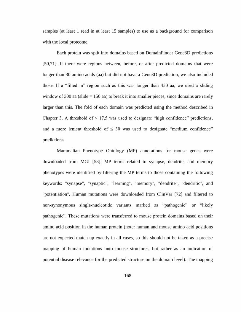
168
samples (at least 1 read in at least 15 samples) to use as a background for comparison
with the local proteome.
Each protein was split into domains based on DomainFinder Gene3D predictions
[50,71]. If there were regions between, before, or after predicted domains that were
longer than 30 amino acids (aa) but did not have a Gene3D prediction, we also included
those. If a “filled in” region such as this was longer than 450 aa, we used a sliding
window of 300 aa (slide = 150 aa) to break it into smaller pieces, since domains are rarely
larger than this. The fold of each domain was predicted using the method described in
Chapter 3. A threshold of ≤ 17.5 was used to designate “high confidence” predictions,
and a more lenient threshold of ≤ 30 was used to designate “medium confidence”
predictions.
Mammalian Phenotype Ontology (MP) annotations for mouse genes were
downloaded from MGI [58]. MP terms related to synapse, dendrite, and memory
phenotypes were identified by filtering the MP terms to those containing the following
keywords: "synapse", "synaptic", "learning", "memory", "dendrite", "dendritic", and
"potentiation". Human mutations were downloaded from ClinVar [72] and filtered to
non-synonymous single-nucleotide variants marked as “pathogenic” or “likely
pathogenic”. These mutations were transferred to mouse protein domains based on their
amino acid position in the human protein (note: human and mouse amino acid positions
are not expected match up exactly in all cases, so this should not be taken as a precise
mapping of human mutations onto mouse structures, but rather as an indication of
potential disease relevance for the predicted structure on the domain level). The mapping

169
between human and mouse orthologous proteins was obtained from the International
Mouse Phenotyping Consortium website (http://www.mousephenotype.org/).
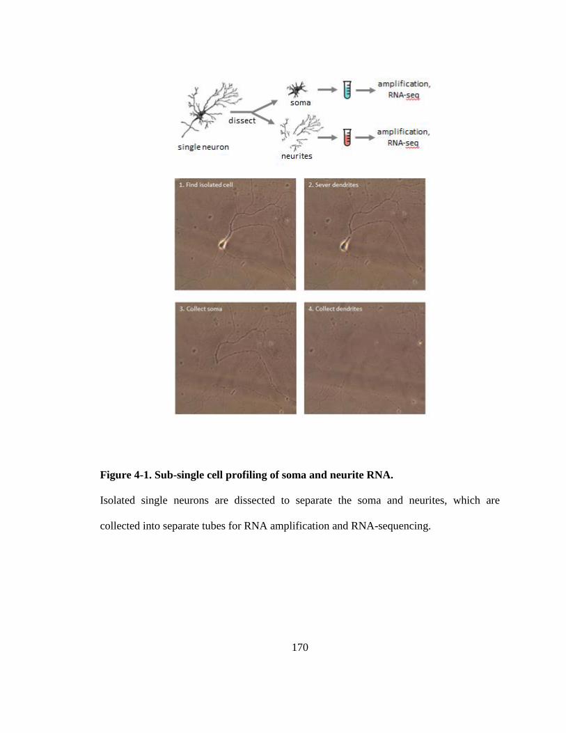
170
Figure 4-1. Sub-single cell profiling of soma and neurite RNA.
Isolated single neurons are dissected to separate the soma and neurites, which are
collected into separate tubes for RNA amplification and RNA-sequencing.
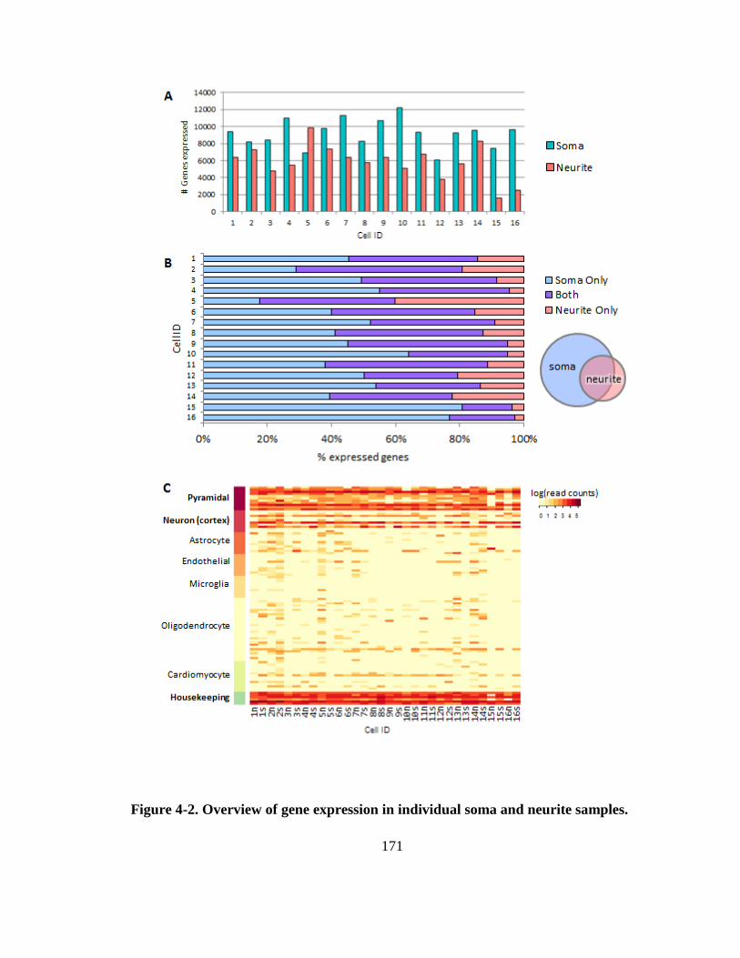
171
Figure 4-2. Overview of gene expression in individual soma and neurite samples.
172
(A) Number of genes expressed per sample with at least 10 reads. (B) Overlap of
expressed genes (≥10 reads) between soma and neurites from the same original cell. (C)
Marker gene expression for several brain cell types. Samples (columns) are indicated by
their cell number and “s” for somas and “n” for neurites. As expected, pyramidal neuron
markers were highly expressed. Cardiomyocte markers are included as a cell type very
unlikely to be present in our cultures and/or confused for a neuron, in order to
demonstrate that low/medium expression of other cell type markers is normal.

173
Figure 4-3. Differentially expressed genes between soma and neurites.
(A) Mean gene normalized counts vs log fold change between neurites and soma.
Significantly differentially expressed genes are shown in red. (B) Overlap between
neurite-enriched genes and previously annotated dendritic genes. (C) Selected GO terms
enriched in the soma- and neurite-enriched gene lists.

174
Figure 4-4. Consistently observed genes in the neurites.
(A) Overlap between consistent-neurite genes and the known dendritic genes. (B)
Selected GO terms enriched among the consistent-neurite genes.
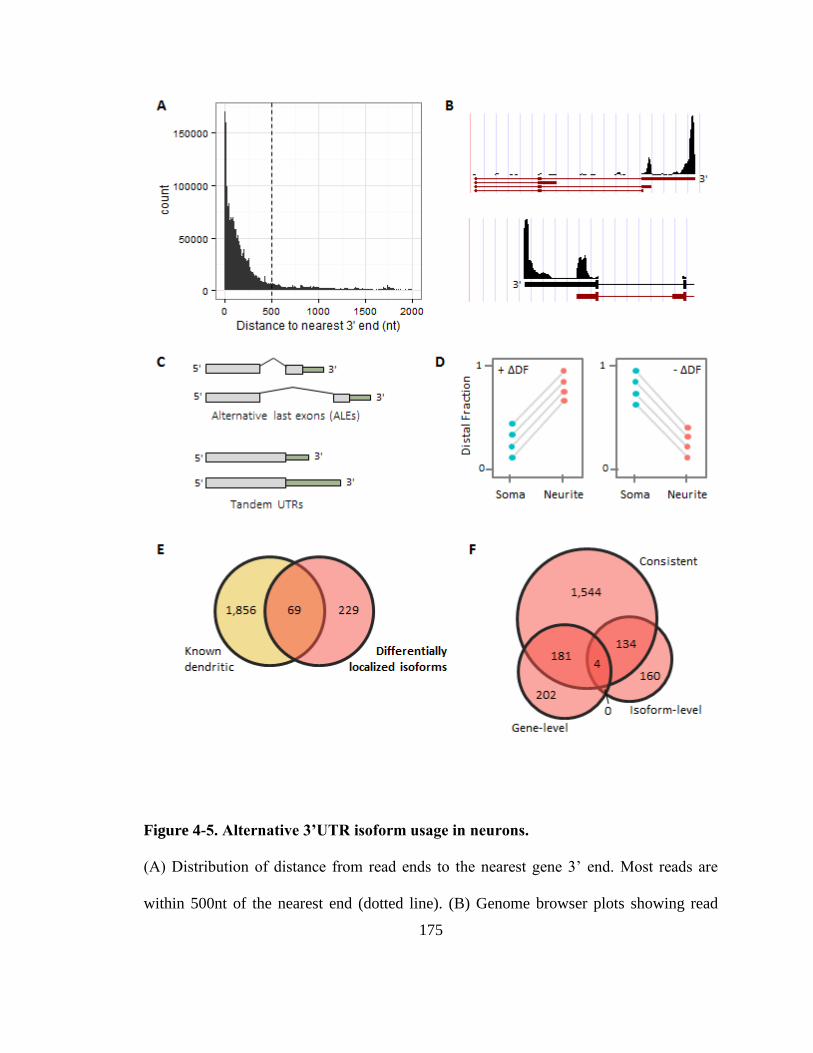
175
Figure 4-5. Alternative 3’UTR isoform usage in neurons.
(A) Distribution of distance from read ends to the nearest gene 3’ end. Most reads are
within 500nt of the nearest end (dotted line). (B) Genome browser plots showing read
176
pileups over two genes. Reads show clear peaks marking the 3’ ends. (C) Definition of
ALEs and Tandem UTRs. (D) Theoretical examples of genes with consistent changes in
distal fraction (ΔDF) across cells, shown as paired plots. Somas and neurites from the
same original cell are shown connected by a line. Consistently positive (left) or negative
(right) ΔDF indicates differentially localized isoforms between the two compartments.
(E) Overlap of differentially localized isoforms with the list of previously annotated
dendritic genes. (F) Overlap between the three sets of neurite-localized genes (gene-level,
consistent, and isoform-level).

177
Figure 4-6. Examples of genes with significantly differentially localized 3’ isoforms.
Paired plots on the left show the DF for each soma-neurite pair (connected by gray lines).
The genome browser plots on the right show the read pile-ups for somas (top track; black
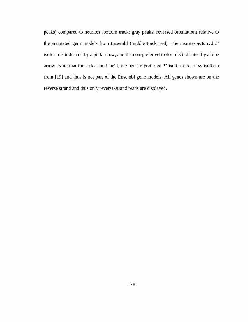
178
peaks) compared to neurites (bottom track; gray peaks; reversed orientation) relative to
the annotated gene models from Ensembl (middle track; red). The neurite-preferred 3’
isoform is indicated by a pink arrow, and the non-preferred isoform is indicated by a blue
arrow. Note that for Uck2 and Ube2i, the neurite-preferred 3’ isoform is a new isoform
from [19] and thus is not part of the Ensembl gene models. All genes shown are on the
reverse strand and thus only reverse-strand reads are displayed.
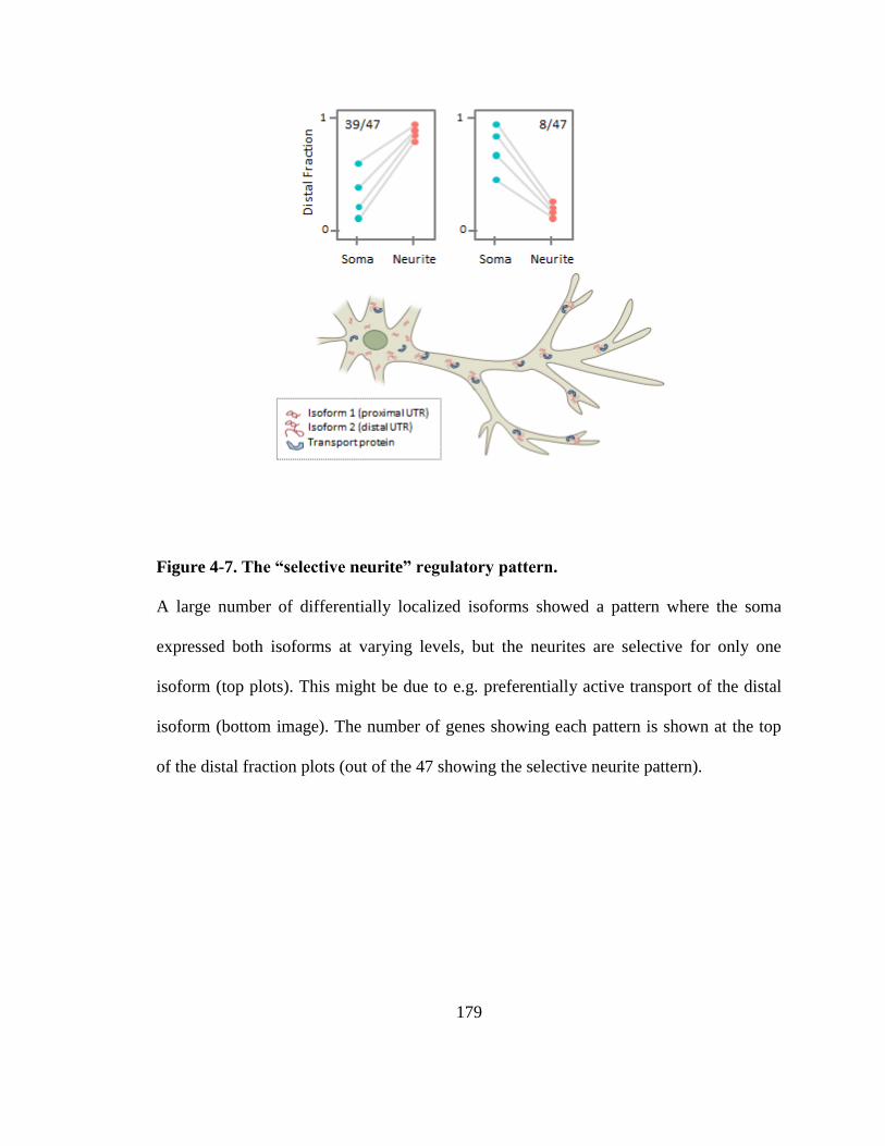
179
Figure 4-7. The “selective neurite” regulatory pattern.
A large number of differentially localized isoforms showed a pattern where the soma
expressed both isoforms at varying levels, but the neurites are selective for only one
isoform (top plots). This might be due to e.g. preferentially active transport of the distal
isoform (bottom image). The number of genes showing each pattern is shown at the top
of the distal fraction plots (out of the 47 showing the selective neurite pattern).

180
Figure 4-8. Potential GA-KT motifs formed by B1 and B2 SINE hairpins in
localized genes.
(A) Consensus structure for the B1 hairpin from a multiple alignment of matches among
the localized genes. Structure was modified to show pairing of G-A/A-G at the putative
GA-KT motif (dashed box). (B) Same as (A), but for the B2 hairpin. Arrow indicates the
U-bulge, similar to the nuclear export signal found in the BC1 hairpin [46,47]. (C)
181
Comparison of the B1 and B2 putative GA-KT elements with the classic GA-KT and the
one found in the BC1/ID element [46,47]. Structure images generated using Forna [73].
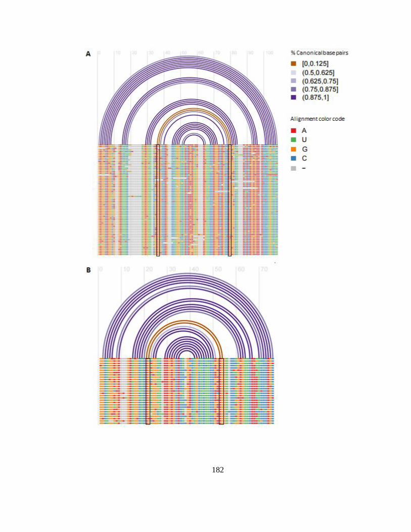
182
183
Figure 4-9. Conserved structure and G-A/A-G pairs in B1 and B2 hairpins in
localized genes.
(A) Multiple alignment of instances of the B1 SINE hairpin found in localized genes. All
matches from the gene-level list are shown. Arches show predicted paired bases and are
colored by percent compatible canonical base pairs. G-A/A-G base pairs are non-
canonical and thus the arches for that pair are shown in brown. Boxes show the G-A/A-G
positions in the alignment. (B) Same as (A), but for the B2 hairpin. Plots generated using
R-chie [74].

184
Figure 4-10. Comparison of the most common structural folds represented in
different proteome sets.
Folds labeled on the left correspond to the top folds in the human proteome, sorted by
rank. The change in rank of each fold from the human proteome to the mouse local
proteome (and from the local proteome to the whole-neuron proteome) is indicated by the
shifted order of the colored circles, connected by lines. Numbers in circles represent the
percent of domains predicted to have that fold in each proteome set. Only high-
confidence predictions were used to calculate rank and percentages.

185
Figure 4-10. Protein structures of the locally-translated proteome.
(A) SCOP folds enriched in the locally translated proteins compared to the neuron-
expressed proteins as a whole. The number of predicted domains in the local proteome

186
for each fold is shown to the right of the bar. (B) Two-dimensional representation of the
protein structure space occupied by neuronally-expressed protein domains. All
neuronally-expressed protein domains are shown in gray in the background, and locally-
translated protein domains are shown in the forefront colored by predicted fold (note that
multiple folds may have similar colors due to the large number of folds). Locally
translated proteins cover most of the structure space spanned by the whole-neuron set.
Projection generated by t-Distributed Stochastic Neighbor Embedding (tSNE) of the
PESS coordinates of each input domain. (C) Same as (B), but overlaying only the local
proteins that overlap the curated list of previously identified dendritic genes.

187
Table 4-1. Neurite-localized genes based on differential expression.
2010016I18Rik Atad2 Fam101b Gm13339 Gm8730 Myeov2 Rpl29 Slc28a3
2010107E04Rik Atp5e Foxp2 Gm13340 Gm9006 Ndnf Rpl31 Slc7a11
2010109I03Rik Atp5j2 Fth1 Gm13341 Gm9843 Ndufa1 Rpl31-ps8 Slco1a1
2810459M11Rik Atp5k Ftl1 Gm13421 Gm9901 Ndufa12 Rpl32 Slfn8
4833422C13Rik Atp5l Gabra4 Gm13433 Gpc6 Ndufa2 Rpl34 Snhg10
4930451C15Rik Atpif1 Gbp7 Gm13488 Gpr35 Ndufa4 Rpl35 Snhg6
5031426D15Rik B430010I23Rik Gli3 Gm13722 Grcc10 Ndufa7 Rpl36a Sp110
5830416I19Rik BC002163 Gltpd2 Gm13826 Gstm1 Ndufb11 Rpl37 Sparc
8430431K14Rik BC051077 Gm10012 Gm13857 GU332589 Ndufb8 Rpl37a Srl
9330159N05Rik BC069931 Gm10033 Gm14303 Hic2 Ndufb9 Rpl38 Sspn
A430106G13Rik Bdnf Gm10059 Gm14450 Invs Ndufv3 Rpl38-ps2 Syt15
A630089N07Rik Bola2 Gm10073 Gm14539 Itga1 Necab1 Rpl39 Tcte1
Acnat2 Brsk1 Gm10076 Gm14586 Itga4 Nhsl2 Rpl39-ps Tfap2b
Aco2 C130026I21Rik Gm10221 Gm14667 Itpr2 Nnat Rpl41 Tirap
Acsm1 Casp4 Gm10222 Gm15393 Jund Nrgn Rplp0 Tmem242
Adamts18 Ccdc141 Gm10263 Gm15462 Kcng3 Nsmf Rplp1 Tnfrsf19
Adap2 Ccnd1 Gm10275 Gm15536 Kcnq5 Oaf Rplp2 Tomm7
Agtrap Ccnd2 Gm10443 Gm16238 Kctd4 Oprd1 Rps10-ps2 Top2a
AK007420 Ccni Gm10485 Gm16416 Kif1a Otc Rps11 Tor4a
AK016170 Cd84 Gm10621 Gm16418 Kif5c Pate2 Rps12 Tpmt
AK020987 Cdk15 Gm10689 Gm16432 Lcn2 Pcdh15 Rps12-ps5 Trim56
AK037411 Chrdl1 Gm10712 Gm17529 Liph Pde1c Rps12-ps9 Trp63
AK037687 Col27a1 Gm11249 Gm17821 Lypd1 Pde2a Rps16-ps2 Tulp1
AK042206 Colec12 Gm11273 Gm2000 Malt1 Pdgfrl Rps17 Uba52
AK048887 Cox4i1 Gm11343 Gm20469 Map1a Phpt1 Rps19 Ugt1a6a
AK051864 Cox5b Gm11407 Gm20541 Map2 Plin3 Rps20 Uqcr10
AK053962 Cox6a1 Gm11408 Gm22567 Mapk8ip1 Pole Rps21 Uqcr11
AK079994 Cox6b1 Gm11410 Gm23134 Mavs Prlr Rps23 Uqcrh
AK133261 Cox6c Gm11477 Gm23368 Mcf2l Prrg1 Rps23-ps Uqcrq
AK134546 Cox7a2 Gm11478 Gm24105 Meis2 Prrx1 Rps24 Usmg5
AK137566 Cox7b Gm11512 Gm24514 Mgst3 Psme2b Rps24-ps3 Vangl1
AK142573 Cox7c Gm11531 Gm26461 Mir682 Ptpn14 Rps25 Vav3
AK142864 Cox8a Gm11808 Gm26870 Mis18bp1 Ptprb Rps25-ps1 Wdr31
AK147589 Ctdspl2 Gm11942 Gm26909 Mre11a Pvalb Rps26 Ybx1
AK153988 Cyp26b1 Gm11956 Gm2830 Mrpl33 Rasgrp4 Rps26-ps1 Zbtb20
AK154552 Dcdc2a Gm11960 Gm3550 mt-Rnr1 Rasl10b Rps28 Zfhx3
AK156971 Ddc Gm12013 Gm4853 mt-Rnr2 Rbm47 Rps29 Zscan20
AK162832 Ddx58 Gm12020 Gm4986 mt-Td Rmi2 Rps5
AK163755 Dock8 Gm12034 Gm5963 mt-Te Romo1 Rpsa
AK164124 DQ072386 Gm12155 Gm6265 mt-Tg Rorb Rpsa-ps10
AK164323 Dtx3l Gm12295 Gm6378 mt-Th RP23-2C22.3 Sepw1
AK169555 Dusp18 Gm12338 Gm6525 mt-Ti Rpl12 Serhl
AK171391 E330033B04Rik Gm12517 Gm7331 mt-Tk Rpl12-ps1 Serpina3k
AK190531 Ebf1 Gm12618 Gm7618 mt-Tl2 Rpl13a Serpine2
AK206180 Egf Gm12778 Gm7866 mt-Tm Rpl19 Shank3
Ankef1 Ern1 Gm12903 Gm8019 mt-Tp Rpl21 Slamf7
Aox3 Esr1 Gm12936 Gm8129 mt-Tq Rpl21-ps12 Slc17a7
Apbb1ip Etv4 Gm12976 Gm8292 mt-Ts1 Rpl21-ps8 Slc17a9
Aqp4 Exo1 Gm13192 Gm8317 mt-Tt Rpl23a Slc22a15
Arhgap31 Exph5 Gm13215 Gm8649 mt-Tw Rpl26 Slc23a1

188
Table 4-2. Consistently observed genes in the neurites.
0610012G03Rik Cacng2 Elk1 Gnal Mrpl43 Ppp2r2c Sdhb Tusc3
1110001J03Rik Cadm1 Elmo1 Gnao1 Mrpl51 Ppp2r5b Sdhc Txn1
1110002L01Rik Cadps Elovl6 Gnaq Mrpl52 Ppp3ca Sdhd Txndc15
1110008F13Rik Calm1 Elp5 Gnas Mrpl9 Ppp6c Sec11c Txndc16
1110008P14Rik Calm2 Emc10 Gnb1 Mrps14 Pptc7 Sec23a Txnl1
1110065P20Rik Calm3 Enah Gnb2l1 Mrps18a Prdx1 Sec23b Txnl4a
1700020I14Rik Caly Enc1 Gng2 Msi2 Prdx2 Sec24a Uba52
1700025G04Rik Camk2b Eno1 Gng3 Mt1 Prdx3 Sec62 Ubash3b
1810043H04Rik Camk2d Eno2 Gnl1 Mt3 Prdx5 Sel1l Ubb
2010003O02Rik Camk2g Enpp5 Gorasp2 Mtch2 Prelid1 Selk Ubc
2010107E04Rik Camk2n2 Ensa Got1 Mtdh Prkaa2 Selm Ube2d2a
2210016L21Rik Camkk2 Eny2 Got2 Mtf1 Prkaca Selt Ube2d3
2410006H16Rik Camsap1 Epb4.1l1 Gpi1 Mtif2 Prkar1a Senp2 Ube2e2
2410015M20Rik Camta1 Epb4.1l3 Gpm6a Mtmr9 Prkar1b Sept11 Ube2h
2610017I09Rik Cand1 Epha5 Gpm6b mt-Rnr1 Prkca Sept3 Ube2l3
2610507B11Rik Canx Epha6 Gpr162 mt-Rnr2 Prmt5 Sept5 Ube2m
2700029M09Rik Capns1 Epm2aip1 Gprasp1 Mtss1l Prpf19 Sept7 Ube2n
2700094K13Rik Capzb Epn1 Gpx1 mt-Td Prpf38b Sepw1 Ube2ql1
2900011O08Rik Casc4 Eps15 Gpx4 mt-Te Prrc2b Serbp1 Ube2r2
2900097C17Rik Caskin1 Erbb4 Grb10 mt-Th Prrc2c Serf2 Ube2z
4932438A13Rik Cbx5 Erc1 Grcc10 mt-Ti Psap Serinc1 Ube3a
5330434G04Rik Cbx6 Erlec1 Gria1 mt-Tm Psd Serinc3 Ubfd1
5730455P16Rik Cby1 Etnk1 Gria2 mt-Tp Psma3 Serp2 Ubl3
6030419C18Rik Ccdc104 Evl Grin1 mt-Tq Psma7 Set Ubl4
6430548M08Rik Ccdc124 Ewsr1 Grin2b mt-Tt Psmb1 Setd7 Ubl5
A030009H04Rik Ccdc127 Exoc5 Grin3a mt-Tw Psmb4 Sez6l2 Ubqln1
A830010M20Rik Ccdc50 Exoc6b Grina Mvb12b Psmb7 Sfi1 Ubqln2
A830039N20Rik Ccdc88a Exoc8 Grip1 Myeov2 Psmc3 Sfxn1 Ubr3
Aak1 Ccnc F830016B08Rik Grk6 Myl12b Psmc5 Sfxn3 Ubxn2a
Aar2 Ccnd2 Fabp3 Grlf1 Myl6 Psmd11 Sgta Uchl1
Aars Ccni Fam115a Grm5 Myo5a Psmd2 Sh3bgrl3 Uck2
Aasdhppt Ccny Fam120a Grpel1 Myt1l Psmd3 Sh3bp5l Ufc1
AB347151 Ccpg1 Fam13c Gsk3b Naa60 Psmd4 Sh3gl2 Ufm1
Abat Ccser2 Fam155a Gstm5 Nap1l5 Psmd8 Sh3glb2 Uhmk1
Abca3 Cct2 Fam168a GU332589 Napa Ptchd4 Shank2 Uhrf1bp1l
Abca5 Cct3 Fam168b Guk1 Napb Ptdss2 Shank3 Uhrf2
Abce1 Cct8 Fam174a H2afz Nav1 Pten Shc3 Ulk2
Abhd17a Cdadc1 Fam195b Habp4 Nav2 Ptges3 Shfm1 Ulk4
Abhd6 Cdc37 Fam19a5 Hadhb Nav3 Ptma Sike1 Unc5c
Abhd8 Cdc37l1 Fam210b Hapln1 Ncald Ptms Sipa1l1 Uqcc2
Abi2 Cdc42 Fam219a Hars Ncam1 Ptp4a2 Ski Uqcr10
Abr Cdc42bpa Fam49a Haus2 Ncaph2 Ptpn4 Skp1a Uqcr11
AC149090.1 Cdc42se2 Fam63b Hcfc1r1 Ncl Ptpn5 Slc1a1 Uqcrb
Acadsb Cdipt Fam73a Hcn1 Ncoa2 Ptprd Slc1a2 Uqcrc1
Acat2 Cdk14 Fam73b Hdac5 Ncor1 Ptprs Slc22a17 Uqcrc2
Aco2 Cdk16 Fam84a Hdac9 Ncs1 Pum2 Slc25a12 Uqcrfs1
Acot7 Cdk4 Fam96b Hdgf Ndfip1 Pura Slc25a22 Uqcrh
Acp1 Cdk5 Fasn Hdgfrp3 Ndn Purb Slc25a23 Uqcrq
Acsl4 Cdk5r1 Fau Hdhd2 Ndrg3 Purg Slc25a3 Usf2
Acsl6 Cdk5r2 Faxc Herc1 Ndrg4 Pvalb Slc25a4 Usmg5
Acss2 Cdkn1b Fbxl16 Herc2 Ndufa1 Pvrl3 Slc25a5 Usp22
Actb Cdr1 Fbxo21 Higd1a Ndufa10 Pxmp4 Slc25a51 Usp32
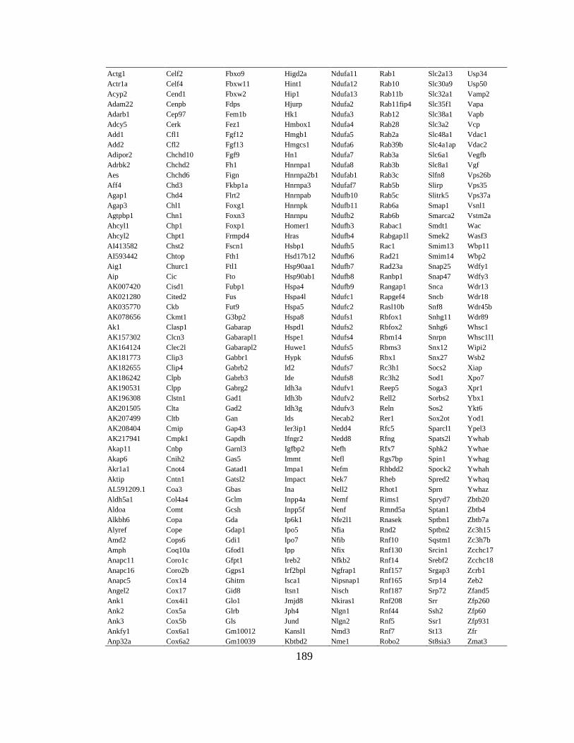
189
Actg1 Celf2 Fbxo9 Higd2a Ndufa11 Rab1 Slc2a13 Usp34
Actr1a Celf4 Fbxw11 Hint1 Ndufa12 Rab10 Slc30a9 Usp50
Acyp2 Cend1 Fbxw2 Hip1 Ndufa13 Rab11b Slc32a1 Vamp2
Adam22 Cenpb Fdps Hjurp Ndufa2 Rab11fip4 Slc35f1 Vapa
Adarb1 Cep97 Fem1b Hk1 Ndufa3 Rab12 Slc38a1 Vapb
Adcy5 Cerk Fez1 Hmbox1 Ndufa4 Rab28 Slc3a2 Vcp
Add1 Cfl1 Fgf12 Hmgb1 Ndufa5 Rab2a Slc48a1 Vdac1
Add2 Cfl2 Fgf13 Hmgcs1 Ndufa6 Rab39b Slc4a1ap Vdac2
Adipor2 Chchd10 Fgf9 Hn1 Ndufa7 Rab3a Slc6a1 Vegfb
Adrbk2 Chchd2 Fh1 Hnrnpa1 Ndufa8 Rab3b Slc8a1 Vgf
Aes Chchd6 Fign Hnrnpa2b1 Ndufab1 Rab3c Slfn8 Vps26b
Aff4 Chd3 Fkbp1a Hnrnpa3 Ndufaf7 Rab5b Slirp Vps35
Agap1 Chd4 Flrt2 Hnrnpab Ndufb10 Rab5c Slitrk5 Vps37a
Agap3 Chl1 Foxg1 Hnrnpk Ndufb11 Rab6a Smap1 Vsnl1
Agtpbp1 Chn1 Foxn3 Hnrnpu Ndufb2 Rab6b Smarca2 Vstm2a
Ahcyl1 Chp1 Foxp1 Homer1 Ndufb3 Rabac1 Smdt1 Wac
Ahcyl2 Chpt1 Frmpd4 Hras Ndufb4 Rabgap1l Smek2 Wasf3
AI413582 Chst2 Fscn1 Hsbp1 Ndufb5 Rac1 Smim13 Wbp11
AI593442 Chtop Fth1 Hsd17b12 Ndufb6 Rad21 Smim14 Wbp2
Aig1 Churc1 Ftl1 Hsp90aa1 Ndufb7 Rad23a Snap25 Wdfy1
Aip Cic Fto Hsp90ab1 Ndufb8 Ranbp1 Snap47 Wdfy3
AK007420 Cisd1 Fubp1 Hspa4 Ndufb9 Rangap1 Snca Wdr13
AK021280 Cited2 Fus Hspa4l Ndufc1 Rapgef4 Sncb Wdr18
AK035770 Ckb Fut9 Hspa5 Ndufc2 Rasl10b Snf8 Wdr45b
AK078656 Ckmt1 G3bp2 Hspa8 Ndufs1 Rbfox1 Snhg11 Wdr89
Ak1 Clasp1 Gabarap Hspd1 Ndufs2 Rbfox2 Snhg6 Whsc1
AK157302 Clcn3 Gabarapl1 Hspe1 Ndufs4 Rbm14 Snrpn Whsc1l1
AK164124 Clec2l Gabarapl2 Huwe1 Ndufs5 Rbms3 Snx12 Wipi2
AK181773 Clip3 Gabbr1 Hypk Ndufs6 Rbx1 Snx27 Wsb2
AK182655 Clip4 Gabrb2 Id2 Ndufs7 Rc3h1 Socs2 Xiap
AK186242 Clpb Gabrb3 Ide Ndufs8 Rc3h2 Sod1 Xpo7
AK190531 Clpp Gabrg2 Idh3a Ndufv1 Reep5 Soga3 Xpr1
AK196308 Clstn1 Gad1 Idh3b Ndufv2 Rell2 Sorbs2 Ybx1
AK201505 Clta Gad2 Idh3g Ndufv3 Reln Sos2 Ykt6
AK207499 Cltb Gan Ids Necab2 Rer1 Sox2ot Yod1
AK208404 Cmip Gap43 Ier3ip1 Nedd4 Rfc5 Sparcl1 Ypel3
AK217941 Cmpk1 Gapdh Ifngr2 Nedd8 Rfng Spats2l Ywhab
Akap11 Cnbp Garnl3 Igfbp2 Nefh Rfx7 Sphk2 Ywhae
Akap6 Cnih2 Gas5 Immt Nefl Rgs7bp Spin1 Ywhag
Akr1a1 Cnot4 Gatad1 Impa1 Nefm Rhbdd2 Spock2 Ywhah
Aktip Cntn1 Gatsl2 Impact Nek7 Rheb Spred2 Ywhaq
AL591209.1 Coa3 Gbas Ina Nell2 Rhot1 Sprn Ywhaz
Aldh5a1 Col4a4 Gclm Inpp4a Nemf Rims1 Spryd7 Zbtb20
Aldoa Comt Gcsh Inpp5f Nenf Rmnd5a Sptan1 Zbtb4
Alkbh6 Copa Gda Ip6k1 Nfe2l1 Rnasek Sptbn1 Zbtb7a
Alyref Cope Gdap1 Ipo5 Nfia Rnd2 Sptbn2 Zc3h15
Amd2 Cops6 Gdi1 Ipo7 Nfib Rnf10 Sqstm1 Zc3h7b
Amph Coq10a Gfod1 Ipp Nfix Rnf130 Srcin1 Zcchc17
Anapc11 Coro1c Gfpt1 Ireb2 Nfkb2 Rnf14 Srebf2 Zcchc18
Anapc16 Coro2b Ggps1 Irf2bpl Ngfrap1 Rnf157 Srgap3 Zcrb1
Anapc5 Cox14 Ghitm Isca1 Nipsnap1 Rnf165 Srp14 Zeb2
Angel2 Cox17 Gid8 Itsn1 Nisch Rnf187 Srp72 Zfand5
Ank1 Cox4i1 Glo1 Jmjd8 Nkiras1 Rnf208 Srr Zfp260
Ank2 Cox5a Glrb Jph4 Nlgn1 Rnf44 Ssh2 Zfp60
Ank3 Cox5b Gls Jund Nlgn2 Rnf5 Ssr1 Zfp931
Ankfy1 Cox6a1 Gm10012 Kansl1 Nmd3 Rnf7 St13 Zfr
Anp32a Cox6a2 Gm10039 Kbtbd2 Nme1 Robo2 St8sia3 Zmat3
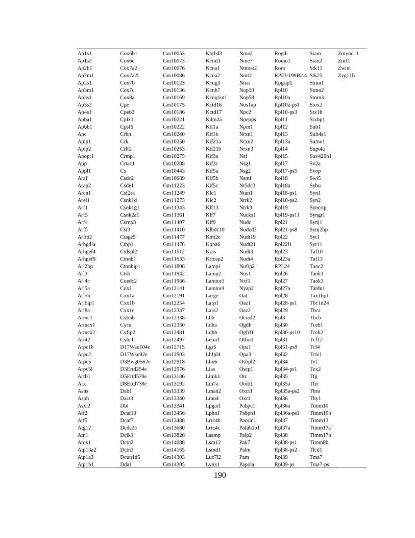
190
Ap1s1 Cox6b1 Gm10053 Kbtbd3 Nme2 Rogdi Stam Zmynd11
Ap1s2 Cox6c Gm10073 Kcmf1 Nme7 Romo1 Stau2 Znrf1
Ap2b1 Cox7a2 Gm10076 Kcna1 Nmnat2 Rora Stk11 Zwint
Ap2m1 Cox7a2l Gm10086 Kcna2 Nmt2 RP23-199B2.4 Stk25 Zyg11b
Ap2s1 Cox7b Gm10123 Kcng3 Nnat Rpgrip1 Stmn1 Ap3m1 Cox7c Gm10136 Kcnh7 Nop10 Rpl10 Stmn2 Ap3s1 Cox8a Gm10169 Kcnq1ot1 Nop58 Rpl10a Stmn3 Ap3s2 Cpe Gm10175 Kctd16 Nos1ap Rpl10a-ps1 Stox2 Ap4s1 Cpeb2 Gm10186 Kctd17 Npc2 Rpl10-ps3 Stx1b Apba1 Cplx1 Gm10221 Kdm2a Npepps Rpl11 Stxbp1 Apbb1 Cpsf6 Gm10222 Kif1a Npm1 Rpl12 Sub1 Apc Crbn Gm10240 Kif1b Nrxn1 Rpl13 Sult4a1 Aplp1 Crk Gm10250 Kif21a Nrxn2 Rpl13a Sumo1 Aplp2 Crlf2 Gm10263 Kif21b Nrxn3 Rpl14 Supt4a Apopt1 Crmp1 Gm10275 Kif3a Nsf Rpl15 Suv420h1 App Crtac1 Gm10288 Kif3c Nsg1 Rpl17 Sv2a Appl1 Cs Gm10443 Kif5a Nsg2 Rpl17-ps5 Svop
Araf Csdc2 Gm10689 Kif5b Nsmf Rpl18 Swi5 Arap2 Csde1 Gm11223 Kif5c Nt5dc3 Rpl18a Sybu Arcn1 Csf2ra Gm11249 Klc1 Ntan1 Rpl18-ps1 Syn1 Arel1 Csnk1d Gm11273 Klc2 Ntrk2 Rpl18-ps2 Syn2 Arf1 Csnk1g1 Gm11343 Klf13 Ntrk3 Rpl19 Syncrip Arf3 Csnk2a1 Gm11361 Klf7 Nucks1 Rpl19-ps11 Syngr1 Arf4 Csrnp3 Gm11407 Klf9 Nudc Rpl21 Synj1 Arf5 Cst3 Gm11410 Klhdc10 Nudcd3 Rpl21-ps8 Synj2bp Arfip2 Ctage5 Gm11477 Kmt2e Nudt19 Rpl22 Syt1 Arhgdia Ctbp1 Gm11478 Kpna6 Nudt21 Rpl22l1 Syt11 Arhgef4 Ctdspl2 Gm11512 Kras Nudt3 Rpl23 Taf10 Arhgef9 Ctnnb1 Gm11633 Krtcap2 Nudt4 Rpl23a Taf13 Arl2bp Ctnnbip1 Gm11808 Lamp1 Nufip2 RPL24 Tanc2 Arl3 Ctsb Gm11942 Lamp2 Nus1 Rpl26 Taok1 Arl4c Cuedc2 Gm11966 Lamtor1 Nxf1 Rpl27 Taok3 Arl5a Cux1 Gm12141 Lamtor4 Nyap2 Rpl27a Tatdn1
Arl5b Cxx1a Gm12191 Large Oat Rpl28 Tax1bp1 Arl6ip1 Cxx1b Gm12254 Larp1 Oaz1 Rpl28-ps1 Tbc1d24 Arl8a Cxx1c Gm12337 Lars2 Oaz2 Rpl29 Tbca Armc1 Cyb5b Gm12338 Lbh Ociad2 Rpl3 Tbcb Armcx1 Cycs Gm12350 Ldha Ogdh Rpl30 Tceb1 Armcx2 Cyfip2 Gm12481 Ldhb Ogfrl1 Rpl30-ps10 Tceb2 Arnt2 Cyhr1 Gm12497 Letm1 Olfm1 Rpl31 Tcf12 Arpc1b D17Wsu104e Gm12715 Lgr5 Opa1 Rpl31-ps8 Tcf4 Arpc2 D17Wsu92e Gm12903 Lhfpl4 Opa3 Rpl32 Tcte1 Arpc5 D3Bwg0562e Gm12918 Lhx6 Osbpl2 Rpl34 Tef Arpc5l D3Ertd254e Gm12976 Lias Oscp1 Rpl34-ps1 Tex2 Arrb1 D5Ertd579e Gm13186 Limk1 Otc Rpl35 Tfg Arx D8Ertd738e Gm13192 Lin7a Otub1 Rpl35a Tfrc Asns Dab1 Gm13339 Lman2 Oxct1 Rpl35a-ps2 Thra Asph Dact3 Gm13340 Lmo4 Oxr1 Rpl36 Thy1 Asxl2 Dbi Gm13341 Lpgat1 Pabpc1 Rpl36a Timm10
Atf2 Dcaf10 Gm13456 Lphn1 Pabpn1 Rpl36a-ps1 Timm10b Atf5 Dcaf7 Gm13488 Lrrc4b Pacsin1 Rpl37 Timm13 Atg12 Dcdc2a Gm13680 Lrrc4c Pafah1b1 Rpl37a Timm17a Atn1 Dclk1 Gm13826 Lsamp Paip2 Rpl38 Timm17b Atox1 Dctn2 Gm14088 Lsm12 Pak7 Rpl38-ps1 Timm8b Atp13a2 Dctn3 Gm14165 Lsmd1 Palm Rpl38-ps2 Tlcd1 Atp1a3 Dcun1d5 Gm14303 Luc7l2 Pam Rpl39 Tma7 Atp1b1 Dda1 Gm14305 Lynx1 Papola Rpl39-ps Tma7-ps

191
Atp2a2 Ddah1 Gm14326 Lyrm9 Parp6 Rpl3-ps1 Tmem130
Atp5a1 Ddx1 Gm14399 Macf1 Parva Rpl4 Tmem132b
Atp5b Ddx3x Gm14450 Maf Pbx1 Rpl41 Tmem135
Atp5c1 Ddx5 Gm14539 Mafg Pcbp2 Rpl5 Tmem14c Atp5d Deaf1 Gm14586 Maged1 Pcdh17 Rpl6 Tmem151b
Atp5e Deb1 Gm14633 Magee1 Pcif1 Rpl7 Tmem167
Atp5f1 Def8 Gm14794 Magi1 Pcmt1 Rpl7a Tmem170b
Atp5g1 Degs2 Gm15421 Map1a Pcmtd1 Rpl8 Tmem178b
Atp5g2 Dennd5a Gm15427 Map1b Pcsk1n Rpl9 Tmem179
Atp5g3 Dennd5b Gm15459 Map1lc3a Pdcd5 Rpl9-ps6 Tmem184c
Atp5h Desi1 Gm15487 Map1lc3b Pdcd6 Rplp0 Tmem234
Atp5j Dgcr6 Gm15500 Map2 Pde11a Rplp1 Tmem242
Atp5j2 Dgkg Gm15501 Map2k2 Pde4a Rplp2 Tmem245
Atp5k Dhx15 Gm15536 Map2k4 Pde4d Rprd2 Tmem256
Atp5l Dhx9 Gm15772 Map3k10 Pdgfa Rps10 Tmem258
Atp5l2 Diras1 Gm15920 Map3k12 Pdha1 Rps10-ps2 Tmem259
Atp5o Disp2 Gm16418 Map4 Pdhx Rps11 Tmem29
Atp6ap1 Dlc1 Gm1673 Map7d1 Pdpk1 Rps11-ps1 Tmem30a
Atp6ap2 Dld Gm17257 Mapk1 Pdxk Rps12 Tmem41b
Atp6v0a1 Dlg2 Gm17383 Mapk10 Pea15a Rps12-ps9 Tmem50b
Atp6v0d1 Dlg4 Gm1821 Mapk3 Pebp1 Rps13 Tmem55a
Atp6v0e2 Dlgap1 Gm2000 Mapk6 Peg3 Rps13-ps1 Tmem55b
Atp6v1a Dlgap2 Gm23134 Mapk8ip1 Pfdn1 Rps13-ps2 Tmem59l Atp6v1b2 Dlgap4 Gm2382 Mapk8ip3 Pfdn2 Rps14 Tmem66 Atp6v1c1 Dlst Gm24105 Mapk9 Pfdn5 Rps15 Tmod2 Atp6v1d Dlx1os Gm26384 Mapre1 Pfkm Rps15a Tmsb10 Atp6v1e1 Dlx6os1 Gm26461 Mapre2 Pfkp Rps15a-ps6 Tmsb4x Atp6v1f Dmd Gm26582 Mapt Pfn1 Rps16 Tmx4 Atp6v1g1 Dnaaf2 Gm26631 March5 Pfn2 Rps16-ps2 Tnks2 Atp6v1g2 Dnajb14 Gm26870 Marcks Pgam1 Rps17 Tnpo1 Atp9a Dnajb6 Gm26909 Mau2 Pgam1-ps2 Rps18 Tnrc6a Atpif1 Dnajc27 Gm26924 Mbd5 Pggt1b Rps19 Tom1l2 Atxn1 Dnajc5 Gm2830 Mbnl2 Pgk1 Rps19-ps6 Tomm20
Atxn10 Dnajc6 Gm2962 Mboat7 Pgk1-rs7 Rps2 Tomm40l Atxn2 Dner Gm3244 Mcf2l Pgp Rps20 Tomm5 Atxn7l3b Dnmt3a Gm3362 Mctp1 Phactr1 Rps21 Tomm6 AU019823 Dock8 Gm3550 Mdga2 Phactr3 Rps23 Tomm7 Auh Dos Gm4117 Mdh1 Phb Rps23-ps Top1 AY036118 Dpp3 Gm4149 Mdh2 Phpt1 Rps24 Tox4 B230219D22Rik Dpp8 Gm4459 Me3 Phyhipl Rps24-ps3 Tpi1 B3gat1 DQ690118 Gm4707 Mea1 Phykpl Rps25 Tpm1 B3gat2 Drap1 Gm4735 Mecp2 Pi4ka Rps25-ps1 Tppp B4galt6 Drg1 Gm4853 Med13 Pigq Rps26 Tpt1 Baalc Dtna Gm5121 Mef2c Pik3ca Rps26-ps1 Tpt1-ps3 Bag1 Dtx3 Gm5384 Meg3 Pip4k2b Rps27a Trak1 Basp1 Dusp8 Gm5436 Megf11 Pip5k1a Rps28 Trappc13 BC002163 Dvl1 Gm5506 Mff Pip5k1c Rps29 Trappc2l BC005537 Dvl3 Gm5514 Mfn2 Pitpna Rps3 Trerf1 BC021618 Dync1h1 Gm5526 Mga Pitpnc1 Rps3a1 Trim2
BC029214 Dync1li2 Gm5566 Mgll Pja2 Rps4x Trim32 BC029722 Dynll1 Gm5601 Mgrn1 Pkp4 Rps5 Trim35 BC031181 Dynll2 Gm5805 Mgst3 Plekhb2 Rps6 Trim37 BC069931 Dynlrb1 Gm5844 Mia3 Plin3 Rps6kb1 Trim44 Bcar1 Dynlt1a Gm5963 Mical2 Plxdc2 Rps6-ps4 Trim8 Bcas2 Dynlt1-ps1 Gm6136 Mid1 Pmpca Rps7 Trim9 Bcat1 Dynlt3 Gm6180 Mien1 Pmvk Rps8 Trip4 Bcl11a Dzank1 Gm6222 Mif Pnkd Rps9 Trnp1
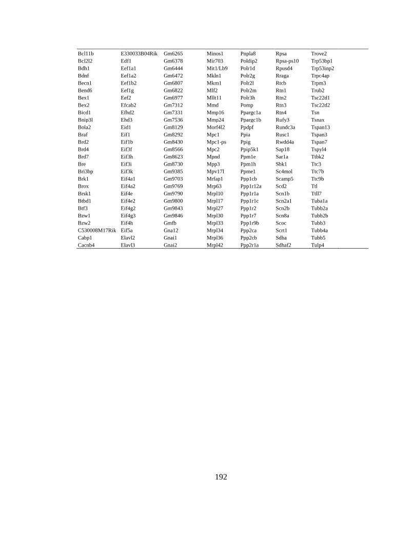
192
Bcl11b E330033B04Rik Gm6265 Minos1 Pnpla8 Rpsa Trove2
Bcl2l2 Edf1 Gm6378 Mir703 Poldip2 Rpsa-ps10 Trp53bp1 Bdh1 Eef1a1 Gm6444 Mit1/Lb9 Polr1d Rpusd4 Trp53inp2
Bdnf Eef1a2 Gm6472 Mkln1 Polr2g Rraga Trpc4ap Becn1 Eef1b2 Gm6807 Mkrn1 Polr2l Rtcb Trpm3 Bend6 Eef1g Gm6822 Mlf2 Polr2m Rtn1 Trub2 Bex1 Eef2 Gm6977 Mllt11 Polr3h Rtn2 Tsc22d1 Bex2 Efcab2 Gm7312 Mmd Pomp Rtn3 Tsc22d2 Bicd1 Efhd2 Gm7331 Mmp16 Ppargc1a Rtn4 Tsn Bnip3l Ehd3 Gm7536 Mmp24 Ppargc1b Rufy3 Tsnax Bola2 Eid1 Gm8129 Morf4l2 Ppdpf Rundc3a Tspan13 Braf Eif1 Gm8292 Mpc1 Ppia Rusc1 Tspan3 Brd2 Eif1b Gm8430 Mpc1-ps Ppig Rwdd4a Tspan7 Brd4 Eif3f Gm8566 Mpc2 Ppip5k1 Sap18 Tspyl4 Brd7 Eif3h Gm8623 Mpnd Ppm1e Sar1a Ttbk2 Bre Eif3i Gm8730 Mpp3 Ppm1h Sbk1 Ttc3 Bri3bp Eif3k Gm9385 Mpv17l Ppme1 Sc4mol Ttc7b
Brk1 Eif4a1 Gm9703 Mrfap1 Ppp1cb Scamp5 Ttc9b Brox Eif4a2 Gm9769 Mrp63 Ppp1r12a Scd2 Ttl Brsk1 Eif4e Gm9790 Mrpl10 Ppp1r1a Scn1b Ttll7 Btbd1 Eif4e2 Gm9800 Mrpl17 Ppp1r1c Scn2a1 Tuba1a Btf3 Eif4g2 Gm9843 Mrpl27 Ppp1r2 Scn2b Tubb2a Bzw1 Eif4g3 Gm9846 Mrpl30 Ppp1r7 Scn8a Tubb2b Bzw2 Eif4h Gmfb Mrpl33 Ppp1r9b Scoc Tubb3 C530008M17Rik Eif5a Gna12 Mrpl34 Ppp2ca Scrt1 Tubb4a Cabp1 Elavl2 Gnai1 Mrpl36 Ppp2cb Sdha Tubb5 Cacnb4 Elavl3 Gnai2 Mrpl42 Ppp2r1a Sdhaf2 Tulp4

193
Table 4-3. Genes with differentially localized 3’UTR isoforms.
2410004B18Rik Capzb Galntl6 Mrpl21 Ppp3cb Slmo1
2700029M09Rik Cbx5 Glud1 Mrpl52 Prkacb Snap91
6430548M08Rik Ccdc47 Gm14204 Mrps23 Prkar1a Snrpa1
A530058N18Rik Ccl27a Gm15459 Mrps33 Prpf38b Snrpb
A830018L16Rik Ccndbp1 Gnai1 Mrps35 Psma6 Snx27
Aak1 Cd99l2 Gnao1 Mrps7 Psmb2 Spag9
Abhd16a Cdc123 Gnb1 Mtch1 Psmc4 Srp72
Abi1 Cdc42 Gps1 mt-Rnr2 Psmd14 Srrm1
AC149090.1 Cdh13 H2afy Myl12b Ptprd Stau1
Acly Cetn2 Haghl Nav2 Purg Stk39
Acss2 Chka Hdac5 Ncam1 Rab11a Suclg1
Actg1 Chmp3 Hint3 Ncbp2 Rab11fip2 Sv2a
Actr2 Cnbp Hnrnpm Ndrg4 Rab21 Syt11
Ahcyl2 Cnot6l Hnrnpu Ndufa10 Rab3a Taf10
Amdhd2 Cog7 Hsd17b12 Ndufa9 Rab4b Taf11
Amfr Commd7 Hsp90aa1 Nsg2 Rabgap1l Tbc1d14
Amph Copg1 Hspa8 Nudc Rac1 Tbcel
Ank2 Cops6 Ift57 Nudt21 Rad23a Tfg
Ankfy1 Csnk1d Inpp4a Nudt3 Ranbp1 Timm10b
Anp32e Csnk2b Inpp5e Nxf1 Rasa1 Tm7sf2
Ap2a2 Cul1 Itpa Nxph1 Rbm17 Tmem126a
Ap2m1 Cxxc4 Jtb Ociad1 Rbm25 Tmem59
Ap3b2 Cyb5 Kalrn Ociad2 Rbms3 Tpm3
Apbb2 Cycs Kcnq2 Ogdh Rer1 Tsnax
Arfgap1 D4Wsu53e Kpna1 Olfm1 Rheb Ttc14
Arid1a Dctn3 Lamtor2 Opcml Rpl15 Tusc3
Arid2 Dctn5 Ldha Oxct1 Rpl21 Uba1
Arl1 Dhdds Lrrc4c Paf1 Rpl27a Ube2e3
Arl16 Dhx30 Lsm3 Paip2 Rpl31 Ube2i
Asnsd1 Dos Lyrm5 Pank1 Rpl5 Ube2j2
Atp5a1 Drg1 Lysmd4 Papolg Rps15a Ube4b
Atp5f1 Dync1i2 Maged2 Pccb Rtfdc1 Ubfd1
Atp5g1 Dynll2 Map1lc3b Pcdh7 Rufy3 Ublcp1
Atp5h E2f6 Map2 Pcgf5 Sap30l Uck2
Atp6v1b2 Ehmt2 Map2k4 Pcmt1 Schip1 Uhrf2
Atxn7l3b Eif2ak1 Map4 Pcmtd1 Scoc Unc5c
Bach1 Emc4 Mapk8ip2 Pcna Sdha Uqcrc2
BC003331 Emc7 Mast1 Pdpk1 Sec14l1 Vamp2
BC005537 Enah Megf11 Pdrg1 Sec24a Vapb
Bcas2 Esf1 Mettl2 Peg3 Selk Vma21
Bcl11a Evi5l Mfap3l Pgk1 Sept11 Vps45
Bdh1 Fam171a1 Minos1 Pigk Sept2 Wasf3
Bex1 Fam229b Mkln1 Pitpnm1 Shisa5 Wdr45b
Bloc1s1 Fam81a Mllt11 Pja2 Skp1a Wipi2
Blzf1 Farsa Mlx Plcb1 Slc1a1 Wsb2
Bsg Fbxo31 Mocs2 Pmpcb Slc25a11 Yif1b
Btf3 Fbxo44 Mpc1 Polr2m Slc25a3 Ywhae
Cacfd1 Fgd4 Mpv17l Ppdpf Slc25a5 Znrf1
Calm3 Flot2 Mrpl10 Ppid Slc25a51
Camk2b Fscn1 Mrpl13 Ppm1h Slc4a3
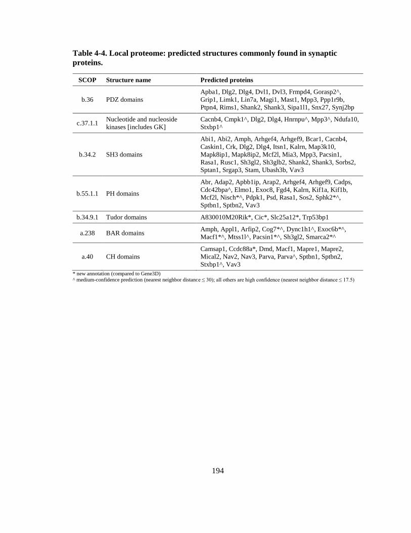
194
Table 4-4. Local proteome: predicted structures commonly found in synaptic
proteins.
SCOP Structure name Predicted proteins
b.36 PDZ domains
Apba1, Dlg2, Dlg4, Dvl1, Dvl3, Frmpd4, Gorasp2^,
Grip1, Limk1, Lin7a, Magi1, Mast1, Mpp3, Ppp1r9b,
Ptpn4, Rims1, Shank2, Shank3, Sipa1l1, Snx27, Synj2bp
c.37.1.1 Nucleotide and nucleoside
kinases [includes GK]
Cacnb4, Cmpk1^, Dlg2, Dlg4, Hnrnpu^, Mpp3^, Ndufa10,
Stxbp1^
b.34.2 SH3 domains
Abi1, Abi2, Amph, Arhgef4, Arhgef9, Bcar1, Cacnb4,
Caskin1, Crk, Dlg2, Dlg4, Itsn1, Kalrn, Map3k10,
Mapk8ip1, Mapk8ip2, Mcf2l, Mia3, Mpp3, Pacsin1,
Rasa1, Rusc1, Sh3gl2, Sh3glb2, Shank2, Shank3, Sorbs2,
Sptan1, Srgap3, Stam, Ubash3b, Vav3
b.55.1.1 PH domains
Abr, Adap2, Apbb1ip, Arap2, Arhgef4, Arhgef9, Cadps,
Cdc42bpa^, Elmo1, Exoc8, Fgd4, Kalrn, Kif1a, Kif1b,
Mcf2l, Nisch*^, Pdpk1, Psd, Rasa1, Sos2, Sphk2*^,
Sptbn1, Sptbn2, Vav3
b.34.9.1 Tudor domains A830010M20Rik*, Cic*, Slc25a12*, Trp53bp1
a.238 BAR domains Amph, Appl1, Arfip2, Cog7*^, Dync1h1^, Exoc6b*^,
Macf1*^, Mtss1l^, Pacsin1*^, Sh3gl2, Smarca2*^
a.40 CH domains
Camsap1, Ccdc88a*, Dmd, Macf1, Mapre1, Mapre2,
Mical2, Nav2, Nav3, Parva, Parva^, Sptbn1, Sptbn2,
Stxbp1^, Vav3
* new annotation (compared to Gene3D) ^ medium-confidence prediction (nearest neighbor distance ≤ 30); all others are high confidence (nearest neighbor distance ≤ 17.5)
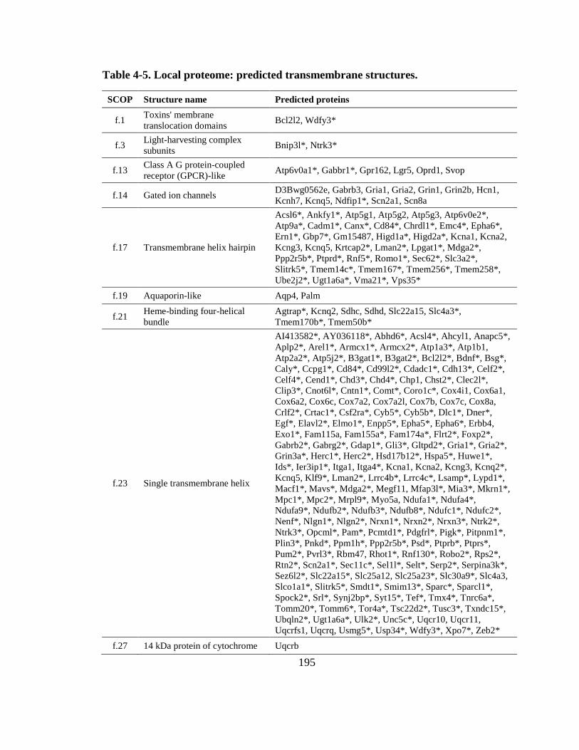
195
Table 4-5. Local proteome: predicted transmembrane structures.
SCOP Structure name Predicted proteins
f.1 Toxins' membrane
translocation domains Bcl2l2, Wdfy3*
f.3 Light-harvesting complex
subunits Bnip3l*, Ntrk3*
f.13 Class A G protein-coupled
receptor (GPCR)-like Atp6v0a1*, Gabbr1*, Gpr162, Lgr5, Oprd1, Svop
f.14 Gated ion channels D3Bwg0562e, Gabrb3, Gria1, Gria2, Grin1, Grin2b, Hcn1,
Kcnh7, Kcnq5, Ndfip1*, Scn2a1, Scn8a
f.17 Transmembrane helix hairpin
Acsl6*, Ankfy1*, Atp5g1, Atp5g2, Atp5g3, Atp6v0e2*,
Atp9a*, Cadm1*, Canx*, Cd84*, Chrdl1*, Emc4*, Epha6*,
Ern1*, Gbp7*, Gm15487, Higd1a*, Higd2a*, Kcna1, Kcna2,
Kcng3, Kcnq5, Krtcap2*, Lman2*, Lpgat1*, Mdga2*,
Ppp2r5b*, Ptprd*, Rnf5*, Romo1*, Sec62*, Slc3a2*,
Slitrk5*, Tmem14c*, Tmem167*, Tmem256*, Tmem258*,
Ube2j2*, Ugt1a6a*, Vma21*, Vps35*
f.19 Aquaporin-like Aqp4, Palm
f.21 Heme-binding four-helical
bundle
Agtrap*, Kcnq2, Sdhc, Sdhd, Slc22a15, Slc4a3*,
Tmem170b*, Tmem50b*
f.23 Single transmembrane helix
AI413582*, AY036118*, Abhd6*, Acsl4*, Ahcyl1, Anapc5*,
Aplp2*, Arel1*, Armcx1*, Armcx2*, Atp1a3*, Atp1b1,
Atp2a2*, Atp5j2*, B3gat1*, B3gat2*, Bcl2l2*, Bdnf*, Bsg*,
Caly*, Ccpg1*, Cd84*, Cd99l2*, Cdadc1*, Cdh13*, Celf2*,
Celf4*, Cend1*, Chd3*, Chd4*, Chp1, Chst2*, Clec2l*,
Clip3*, Cnot6l*, Cntn1*, Comt*, Coro1c*, Cox4i1, Cox6a1,
Cox6a2, Cox6c, Cox7a2, Cox7a2l, Cox7b, Cox7c, Cox8a,
Crlf2*, Crtac1*, Csf2ra*, Cyb5*, Cyb5b*, Dlc1*, Dner*,
Egf*, Elavl2*, Elmo1*, Enpp5*, Epha5*, Epha6*, Erbb4,
Exo1*, Fam115a, Fam155a*, Fam174a*, Flrt2*, Foxp2*,
Gabrb2*, Gabrg2*, Gdap1*, Gli3*, Gltpd2*, Gria1*, Gria2*,
Grin3a*, Herc1*, Herc2*, Hsd17b12*, Hspa5*, Huwe1*,
Ids*, Ier3ip1*, Itga1, Itga4*, Kcna1, Kcna2, Kcng3, Kcnq2*,
Kcnq5, Klf9*, Lman2*, Lrrc4b*, Lrrc4c*, Lsamp*, Lypd1*,
Macf1*, Mavs*, Mdga2*, Megf11, Mfap3l*, Mia3*, Mkrn1*,
Mpc1*, Mpc2*, Mrpl9*, Myo5a, Ndufa1*, Ndufa4*,
Ndufa9*, Ndufb2*, Ndufb3*, Ndufb8*, Ndufc1*, Ndufc2*,
Nenf*, Nlgn1*, Nlgn2*, Nrxn1*, Nrxn2*, Nrxn3*, Ntrk2*,
Ntrk3*, Opcml*, Pam*, Pcmtd1*, Pdgfrl*, Pigk*, Pitpnm1*,
Plin3*, Pnkd*, Ppm1h*, Ppp2r5b*, Psd*, Ptprb*, Ptprs*,
Pum2*, Pvrl3*, Rbm47, Rhot1*, Rnf130*, Robo2*, Rps2*,
Rtn2*, Scn2a1*, Sec11c*, Sel1l*, Selt*, Serp2*, Serpina3k*,
Sez6l2*, Slc22a15*, Slc25a12, Slc25a23*, Slc30a9*, Slc4a3,
Slco1a1*, Slitrk5*, Smdt1*, Smim13*, Sparc*, Sparcl1*,
Spock2*, Srl*, Synj2bp*, Syt15*, Tef*, Tmx4*, Tnrc6a*,
Tomm20*, Tomm6*, Tor4a*, Tsc22d2*, Tusc3*, Txndc15*,
Ubqln2*, Ugt1a6a*, Ulk2*, Unc5c*, Uqcr10, Uqcr11,
Uqcrfs1, Uqcrq, Usmg5*, Usp34*, Wdfy3*, Xpo7*, Zeb2*
f.27 14 kDa protein of cytochrome Uqcrb
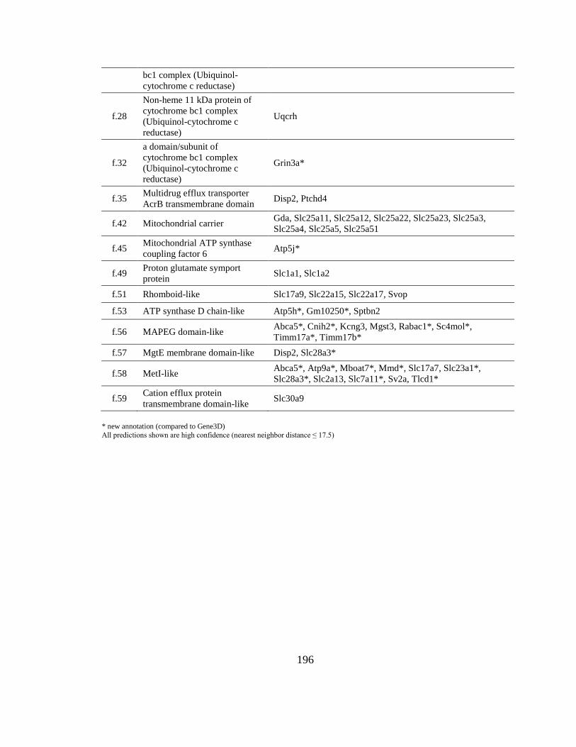
196
bc1 complex (Ubiquinol-
cytochrome c reductase)
f.28
Non-heme 11 kDa protein of
cytochrome bc1 complex
(Ubiquinol-cytochrome c
reductase)
Uqcrh
f.32
a domain/subunit of
cytochrome bc1 complex
(Ubiquinol-cytochrome c
reductase)
Grin3a*
f.35 Multidrug efflux transporter
AcrB transmembrane domain Disp2, Ptchd4
f.42 Mitochondrial carrier Gda, Slc25a11, Slc25a12, Slc25a22, Slc25a23, Slc25a3,
Slc25a4, Slc25a5, Slc25a51
f.45 Mitochondrial ATP synthase
coupling factor 6 Atp5j*
f.49 Proton glutamate symport
protein Slc1a1, Slc1a2
f.51 Rhomboid-like Slc17a9, Slc22a15, Slc22a17, Svop
f.53 ATP synthase D chain-like Atp5h*, Gm10250*, Sptbn2
f.56 MAPEG domain-like Abca5*, Cnih2*, Kcng3, Mgst3, Rabac1*, Sc4mol*,
Timm17a*, Timm17b*
f.57 MgtE membrane domain-like Disp2, Slc28a3*
f.58 MetI-like Abca5*, Atp9a*, Mboat7*, Mmd*, Slc17a7, Slc23a1*,
Slc28a3*, Slc2a13, Slc7a11*, Sv2a, Tlcd1*
f.59 Cation efflux protein
transmembrane domain-like Slc30a9
* new annotation (compared to Gene3D)
All predictions shown are high confidence (nearest neighbor distance ≤ 17.5)

197
Table 4-6. Local proteome: predicted RNA-binding structures.
Fold Desc Predicted proteins
a.144 PABP domain-like Dync1h1*, Pabpc1
a.217 Surp module (SWAP domain) Zc3h7b*
b.38 Sm-like fold Atxn2, Lsm3, Lsmd1, Snrpb, Snrpn
b.40.4 OB-fold; Nucleic acid binding
Ccdc141, Cmip, Csdc2, Csde1, Dlst, Dnaaf2*, Eif5a,
Gm10263, Pdgfrl, Polr2g, Polr3h, Rapgef4, Rpl6, Rps11,
Rps23, Rps28, Trub2*, Ttc14, Ybx1, Zcchc17
d.265 Pseudouridine synthase Rpusd4, Trub2
d.41 alpha/beta-Hammerhead Aox3, Mocs2, Rpl10
d.50 dsRBD-like Adarb1, Dhx9, Rps2, Stau1, Stau2
d.51 Eukaryotic type KH-domain
(KH-domain type I) Fubp1, Hnrnpk, Pcbp2
d.58.7 Canonical RNA binding
domain (RBD) [RRM]
Alyref, Celf2, Celf4, Cnot4, Cpeb2, Cpsf6, Eif4h, Elavl2,
Elavl3, Ewsr1, Fus, G3bp2, Hnrnpa1, Hnrnpa2b1, Hnrnpa3,
Hnrnpab, Hnrnpm, Msi2, Ncbp2, Ncl, Nxf1, Pabpc1,
Pabpn1, Ppargc1a, Ppargc1b, Rbfox1, Rbfox2, Rbm14,
Rbm17, Rbm25, Rbm47, Rbms3, Slirp, Syncrip, Tnrc6a,
Uhmk1, Zcrb1
g.66 CCCH zinc finger Mbnl2, Mkrn1, Rc3h1, Rc3h2, Zc3h15, Zc3h7b
* new annotation (compared to Gene3D)
All predictions shown are high confidence (nearest neighbor distance ≤ 17.5)

198
Table 4-7. New structure predictions for domains with pathogenic variants in
humans and memory/synapse-related phenotypes.
Gene Domain Fold Prediction Phenotypes
App 712-770 [g.41] - Rubredoxin-like abnormal learning/memory/conditioning;abnormal long term
object recognition memory;abnormal long term potentiation;abnormal long term spatial reference
memory;abnormal spatial learning;abnormal spatial reference
memory;abnormal spatial working memory;abnormal synapse morphology;reduced long term potentiation
App^ 452-671 [a.151] - Glutamyl tRNA-
reductase dimerization domain
Arx 396-564 [g.88] - Intrinsically disordered
proteins
abnormal associative learning;abnormal spatial learning
Arx^ 1-326 [a.8] - immunoglobulin/albumin-
binding domain-like
Asns 530-561 [a.118] - alpha-alpha superhelix abnormal long term object recognition memory;abnormal short
term object recognition memory
Atp13a2^ 1-194 [d.14] - Ribosomal protein S5 domain 2-like
abnormal spatial learning;decreased memory-marker CD4-positive NK T cell number
Atp1a3 264-330 [f.23] - Single transmembrane
helix abnormal CNS synaptic transmission;abnormal miniature
inhibitory postsynaptic currents;abnormal spatial learning Atp1a3 386-423 [g.24] - TNF receptor-like
Bdnf 1-134 [f.23] - Single transmembrane
helix
abnormal CNS synaptic transmission;abnormal dendrite
morphology;abnormal dendritic spine morphology;abnormal
excitatory postsynaptic potential;abnormal inhibitory postsynaptic currents;abnormal synaptic plasticity;impaired
synaptic plasticity;reduced long term potentiation
Braf 268-486 [g.37] - beta-beta-alpha zinc fingers
abnormal associative learning;abnormal long term object
recognition memory;abnormal Purkinje cell dendrite morphology;abnormal spatial learning;reduced long term
potentiation
Brd7^ 257-651 [a.7] - Spectrin repeat-like
abnormal dendrite morphology;abnormal long term object
recognition memory;abnormal short term object recognition memory;impaired spatial learning
Ctnnb1 1-134 [b.108] - Triple-stranded beta-
helix
abnormal spatial reference memory;abnormal synaptic vesicle
clustering;reduced long term potentiation
Dcdc2a^ 223-475 [g.3] - Knottins (small
inhibitors, toxins, lectins)
abnormal short term object recognition memory;abnormal
spatial learning;abnormal spatial working memory
Dmd 2128-2172 [a.4] - DNA/RNA-binding 3-helical bundle
abnormal neuromuscular synapse morphology
Dmd 3082-3113 [a.4] - DNA/RNA-binding 3-
helical bundle
Dmd 1775-1813 [a.4] - DNA/RNA-binding 3-
helical bundle
Dmd 1377-1436 [a.60] - SAM domain-like
Dmd 241-341 [b.108] - Triple-stranded beta-
helix
Dmd 671-723 [b.108] - Triple-stranded beta-helix
Dmd 1968-2000 [b.34] - SH3-like barrel
Dmd 905-944 [d.198] - Secretion chaperone-like
Dmd 3286-3490 [g.39] - Glucocorticoid receptor-
like (DNA-binding domain)
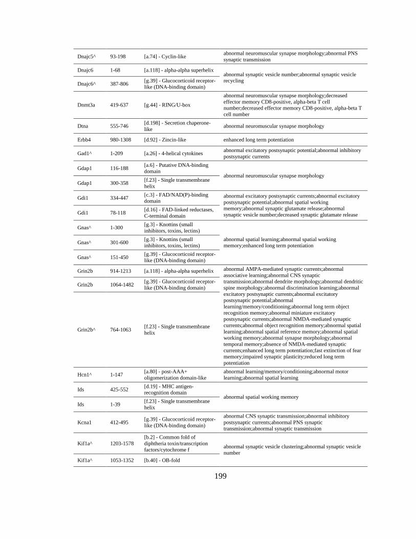
199
Dnajc5^ 93-198 [a.74] - Cyclin-like abnormal neuromuscular synapse morphology;abnormal PNS
synaptic transmission
Dnajc6 1-68 [a.118] - alpha-alpha superhelix abnormal synaptic vesicle number;abnormal synaptic vesicle recycling
Dnajc6^ 387-806 [g.39] - Glucocorticoid receptor-
like (DNA-binding domain)
Dnmt3a 419-637 [g.44] - RING/U-box
abnormal neuromuscular synapse morphology;decreased
effector memory CD8-positive, alpha-beta T cell number;decreased effector memory CD8-positive, alpha-beta T
cell number
Dtna 555-746 [d.198] - Secretion chaperone-
like abnormal neuromuscular synapse morphology
Erbb4 980-1308 [d.92] - Zincin-like enhanced long term potentiation
Gad1^ 1-209 [a.26] - 4-helical cytokines abnormal excitatory postsynaptic potential;abnormal inhibitory
postsynaptic currents
Gdap1 116-188 [a.6] - Putative DNA-binding
domain abnormal neuromuscular synapse morphology
Gdap1 300-358 [f.23] - Single transmembrane
helix
Gdi1 334-447 [c.3] - FAD/NAD(P)-binding domain
abnormal excitatory postsynaptic currents;abnormal excitatory
postsynaptic potential;abnormal spatial working memory;abnormal synaptic glutamate release;abnormal
synaptic vesicle number;decreased synaptic glutamate release Gdi1 78-118 [d.16] - FAD-linked reductases,
C-terminal domain
Gnas^ 1-300 [g.3] - Knottins (small
inhibitors, toxins, lectins)
abnormal spatial learning;abnormal spatial working memory;enhanced long term potentiation
Gnas^ 301-600 [g.3] - Knottins (small inhibitors, toxins, lectins)
Gnas^ 151-450 [g.39] - Glucocorticoid receptor-
like (DNA-binding domain)
Grin2b 914-1213 [a.118] - alpha-alpha superhelix abnormal AMPA-mediated synaptic currents;abnormal
associative learning;abnormal CNS synaptic transmission;abnormal dendrite morphology;abnormal dendritic
spine morphology;abnormal discrimination learning;abnormal
excitatory postsynaptic currents;abnormal excitatory postsynaptic potential;abnormal
learning/memory/conditioning;abnormal long term object
recognition memory;abnormal miniature excitatory postsynaptic currents;abnormal NMDA-mediated synaptic
currents;abnormal object recognition memory;abnormal spatial
learning;abnormal spatial reference memory;abnormal spatial working memory;abnormal synapse morphology;abnormal
temporal memory;absence of NMDA-mediated synaptic
currents;enhanced long term potentiation;fast extinction of fear memory;impaired synaptic plasticity;reduced long term
potentiation
Grin2b 1064-1482 [g.39] - Glucocorticoid receptor-
like (DNA-binding domain)
Grin2b^ 764-1063 [f.23] - Single transmembrane
helix
Hcn1^ 1-147 [a.80] - post-AAA+
oligomerization domain-like
abnormal learning/memory/conditioning;abnormal motor
learning;abnormal spatial learning
Ids 425-552 [d.19] - MHC antigen-recognition domain
abnormal spatial working memory
Ids 1-39 [f.23] - Single transmembrane
helix
Kcna1 412-495 [g.39] - Glucocorticoid receptor-
like (DNA-binding domain)
abnormal CNS synaptic transmission;abnormal inhibitory
postsynaptic currents;abnormal PNS synaptic transmission;abnormal synaptic transmission
Kif1a^ 1203-1578
[b.2] - Common fold of
diphtheria toxin/transcription
factors/cytochrome f abnormal synaptic vesicle clustering;abnormal synaptic vesicle
number
Kif1a^ 1053-1352 [b.40] - OB-fold

200
Kif1b^ 1093-1392 [b.1] - Immunoglobulin-like
beta-sandwich
abnormal synaptic vesicle number Kif1b^ 1243-1542
[b.2] - Common fold of
diphtheria toxin/transcription factors/cytochrome f
Kif1b^ 1393-1699 [d.3] - Cysteine proteinases
Kif1b^ 643-942 [d.43] - EF-Ts domain-like
Mapk8ip1^ 1-300 [g.3] - Knottins (small
inhibitors, toxins, lectins) abnormal NMDA-mediated synaptic currents
Mapt 301-733 [g.37] - beta-beta-alpha zinc fingers
abnormal dendrite morphology;abnormal long term object recognition memory;abnormal motor learning;abnormal spatial
learning;abnormal spatial working memory;enhanced spatial
learning;reduced long term potentiation Mapt^ 1-300 [g.3] - Knottins (small
inhibitors, toxins, lectins)
Mbd5^ 1-300 [d.169] - C-type lectin-like abnormal associative learning;abnormal dendrite morphology;abnormal excitatory postsynaptic
currents;abnormal excitatory postsynaptic potential;abnormal
learning/memory/conditioning;abnormal long term object recognition memory;abnormal miniature excitatory
postsynaptic currents;abnormal miniature inhibitory
postsynaptic currents;abnormal motor learning;abnormal spatial learning;abnormal synaptic vesicle number;decreased CNS
synapse formation;reduced long term potentiation
Mecp2^ 196-484 [g.3] - Knottins (small
inhibitors, toxins, lectins)
Mecp2^ 1-66 [g.39] - Glucocorticoid receptor-like (DNA-binding domain)
Mfn2 314-363 [a.6] - Putative DNA-binding
domain
abnormal Purkinje cell dendrite morphology Mfn2 1-84 [a.60] - SAM domain-like
Mfn2^ 430-694 [a.211] - HD-domain/PDEase-
like
Mid1 496-680 [b.29] - Concanavalin A-like lectins/glucanases abnormal learning/memory/conditioning;abnormal motor
learning Mid1^ 216-380 [a.7] - Spectrin repeat-like
Nfkb2 850-899 [g.39] - Glucocorticoid receptor-
like (DNA-binding domain)
abnormal myeloid dendritic cell morphology;abnormal spleen
follicular dendritic cell network;decreased dendritic cell
number;decreased myeloid dendritic cell number;increased
plasmacytoid dendritic cell number
Ntrk2 376-530 [f.23] - Single transmembrane
helix
abnormal avoidance learning behavior;abnormal dendrite morphology;abnormal excitatory postsynaptic
potential;abnormal learning/memory/conditioning;abnormal
long term potentiation;abnormal Purkinje cell dendrite morphology;abnormal spatial learning;abnormal spatial
working memory;abnormal synapse morphology;impaired
synaptic plasticity;reduced long term potentiation
Otc 1-31 [d.92] - Zincin-like abnormal dendrite morphology;abnormal spatial learning;abnormal spatial reference memory;abnormal spatial
working memory
Pafah1b1 1-100
[a.221] - Lissencephaly-1
protein (Lis-1, PAF-AH alpha) N-terminal domain
abnormal spatial learning
Pnkd 1-116 [f.23] - Single transmembrane
helix
abnormal synaptic dopamine release;abnormal synaptic
transmission
Psap 394-436 [a.118] - alpha-alpha superhelix
reduced long term potentiation Psap^ 1-58 [g.24] - TNF receptor-like
Pten 354-403 [g.37] - beta-beta-alpha zinc fingers
abnormal CNS synaptic transmission;abnormal dendrite morphology;abnormal dendritic spine morphology;abnormal
excitatory postsynaptic currents;abnormal excitatory
postsynaptic potential;abnormal miniature excitatory Pten 283-313 [g.5] - Midkine

201
postsynaptic currents;abnormal Purkinje cell dendrite
morphology;abnormal synapse morphology;abnormal synaptic
depression;abnormal synaptic transmission;abnormal synaptic vesicle number;impaired spatial learning
Pura^ 1-321 [d.198] - Secretion chaperone-
like decreased CNS synapse formation
Reln 3135-3228 [b.121] - Nucleoplasmin-
like/VP (viral coat and capsid) abnormal short term spatial reference memory
Rims1^ 704-1003 [g.3] - Knottins (small inhibitors, toxins, lectins)
abnormal CNS synaptic transmission;abnormal excitatory postsynaptic currents;abnormal excitatory postsynaptic
potential;abnormal inhibitory postsynaptic currents;abnormal
post-tetanic potentiation;impaired synaptic plasticity;reduced long term potentiation
Robo2 1164-1470 [a.118] - alpha-alpha superhelix
abnormal Purkinje cell dendrite morphology Robo2 864-1163 [f.23] - Single transmembrane
helix
Robo2^ 1014-1313 [g.3] - Knottins (small
inhibitors, toxins, lectins)
Scn8a 1468-1518 [d.372] - YqaI-like
abnormal neuromuscular synapse morphology Scn8a^ 417-750 [d.58] - Ferredoxin-like
Scn8a^ 980-1200 [d.6] - Prion-like
Shank3 531-568 [b.72] - WW domain-like abnormal CNS synaptic transmission;abnormal dendritic spine morphology;abnormal excitatory postsynaptic
currents;abnormal excitatory postsynaptic potential;abnormal
long term object recognition memory;abnormal miniature excitatory postsynaptic currents;abnormal miniature inhibitory
postsynaptic currents;abnormal motor learning;abnormal object
recognition memory;abnormal spatial learning;abnormal spatial reference memory;abnormal synapse morphology;abnormal
synaptic transmission;decreased excitatory postsynaptic current
amplitude;decreased post-tetanic potentiation;decreased synaptic depression;impaired learning;impaired spatial
learning;impaired synaptic plasticity;reduced long term
potentiation;reduced NMDA-mediated synaptic currents
Shank3^ 963-1262 [g.39] - Glucocorticoid receptor-
like (DNA-binding domain)
Shank3^ 1113-1412 [g.39] - Glucocorticoid receptor-
like (DNA-binding domain)
Slc6a1^ 151-599 [f.13] - Class A G protein-coupled receptor (GPCR)-like abnormal inhibitory postsynaptic currents;abnormal object
recognition memory;abnormal spatial working memory Slc6a1^ 1-300
[f.21] - Heme-binding four-
helical bundle
Stxbp1^ 324-361 [a.43] - Ribbon-helix-helix abnormal synaptic transmission
Syn1^ 393-706 [g.37] - beta-beta-alpha zinc
fingers
abnormal CNS synapse formation;abnormal excitatory
postsynaptic potential;abnormal inhibitory postsynaptic
currents;abnormal synaptic vesicle clustering;abnormal synaptic vesicle recycling;delayed CNS synapse formation;increased
synaptic depression
Synj1^ 1-300 [b.50] - Acid proteases
increased synaptic depression
Synj1^ 151-513 [c.55] - Ribonuclease H-like
motif
Tcf4^ 151-556 [g.3] - Knottins (small
inhibitors, toxins, lectins) abnormal associative learning;impaired spatial learning
Tcf4^ 1-300 [g.39] - Glucocorticoid receptor-like (DNA-binding domain)
Thra 376-492 [a.4] - DNA/RNA-binding 3-
helical bundle abnormal object recognition memory;abnormal Purkinje cell
dendrite morphology Thra 1-51
[g.3] - Knottins (small
inhibitors, toxins, lectins)

202
Ube3a 721-755 [b.108] - Triple-stranded beta-
helix abnormal dendrite morphology;abnormal
learning/memory/conditioning;abnormal long term potentiation;abnormal motor learning;abnormal spatial
learning;reduced long term potentiation
Ube3a^ 151-499 [a.288] - UraD-like
Ube3a^ 1-300 [d.389] - Menin N-terminal
domain-like
^ medium-confidence prediction (nearest neighbor distance ≤ 30); all others are high confidence (nearest neighbor distance ≤ 17.5)
All are new annotations (compared to Gene3D)

203
4.5 References
1 Martin, K.C. et al. (2000) Local protein synthesis and its role in synapse-specific
plasticity. Curr. Opin. Neurobiol. 10, 587–592
2 Miyashiro, K. et al. (1994) On the nature and differential distribution of mRNAs in
hippocampal neurites: implications for neuronal functioning. Proc. Natl. Acad. Sci.
U. S. A. 91, 10800–4
3 Moccia, R. et al. (2003) An unbiased cDNA library prepared from isolated Aplysia
sensory neuron processes is enriched for cytoskeletal and translational mRNAs. J.
Neurosci. 23, 9409–17
4 Zhong, J. et al. (2006) Dendritic mRNAs encode diversified functionalities in
hippocampal pyramidal neurons. BMC Neurosci. 7, 17
5 Poon, M.M. et al. (2006) Identification of process-localized mRNAs from cultured
rodent hippocampal neurons. J. Neurosci. 26, 13390–9
6 Suzuki, T. et al. (2007) Characterization of mRNA species that are associated with
postsynaptic density fraction by gene chip microarray analysis. Neurosci. Res. 57,
61–85
7 Cajigas, I.J. et al. (2012) The local transcriptome in the synaptic neuropil revealed
by deep sequencing and high-resolution imaging. Neuron 74, 453–66
8 Ainsley, J.A. et al. (2014) Functionally diverse dendritic mRNAs rapidly associate
with ribosomes following a novel experience. Nat. Commun. 5, 4510
9 Francis, C. et al. (2014) Divergence of RNA localization between rat and mouse
neurons reveals the potential for rapid brain evolution. BMC Genomics 15, 883
10 Taliaferro, J.M. et al. (2016) Distal Alternative Last Exons Localize mRNAs to
Neural Projections. Mol. Cell 61, 821–833
11 Lovatt, D. et al. (2014) Transcriptome in vivo analysis (TIVA) of spatially defined
single cells in live tissue. Nat. Methods 11, 190–6
12 Lubeck, E. et al. (2014) Single-cell in situ RNA profiling by sequential
hybridization. Nat. Methods 11, 360–1
13 Lee, J.H. et al. (2014) Highly Multiplexed Subcellular RNA Sequencing in Situ.
Science 1360,

204
14 Chen, K.H. et al. (2015) Spatially resolved, highly multiplexed RNA profiling in
single cells. Science 1363, 1360–1363
15 Dueck, H. et al. (2015) Deep sequencing reveals cell-type-specific patterns of
single-cell transcriptome variation. Genome Biol. 16, 122
16 Bramham, C.R. and Wells, D.G. (2007) Dendritic mRNA: transport, translation
and function. Nat. Rev. Neurosci. 8, 776–789
17 Gerstberger, S. et al. (2014) A census of human RNA-binding proteins. Nat. Rev.
Genet. 15, 829–845
18 Buckley, P.T. et al. (2011) Cytoplasmic intron sequence-retaining transcripts can
be dendritically targeted via ID element retrotransposons. Neuron 69, 877–84
19 Miura, P. et al. (2013) Widespread and extensive lengthening of 3’ UTRs in the
mammalian brain. Genome Res. 23, 812–25
20 Miller, S. et al. (2002) Disruption of Dendritic Translation of CaMKIIα Impairs
Stabilization of Synaptic Plasticity and Memory Consolidation. Neuron 36, 507–
519
21 Timmons, J. a. et al. (2015) Multiple sources of bias confound functional
enrichment analysis of global -omics data. Genome Biol. 16, 186
22 Kim, E. and Sheng, M. (2004) PDZ domain proteins of synapses. Nat. Rev.
Neurosci. 5, 771–781
23 Dalva, M.B. et al. (2007) Cell adhesion molecules: signalling functions at the
synapse. Nat. Rev. Neurosci. 8, 206–220
24 Zheng, C.-Y. et al. (2011) MAGUKs, Synaptic Development, and Synaptic
Plasticity. Neurosci. 17, 493–512
25 Liu-Yesucevitz, L. et al. (2011) Local RNA translation at the synapse and in
disease. J. Neurosci. 31, 16086–93
26 Grant, S.G. (2012) Synaptopathies: diseases of the synaptome. Curr. Opin.
Neurobiol. 22, 522–529
27 Love, M.I. et al. (2014) Moderated estimation of fold change and dispersion for
RNA-seq data with DESeq2. Genome Biol. 15, 550
28 Miura, P. et al. (2014) Alternative polyadenylation in the nervous system: To what
lengths will 3’ UTR extensions take us? Bioessays DOI: 10.1002/bies.201300174
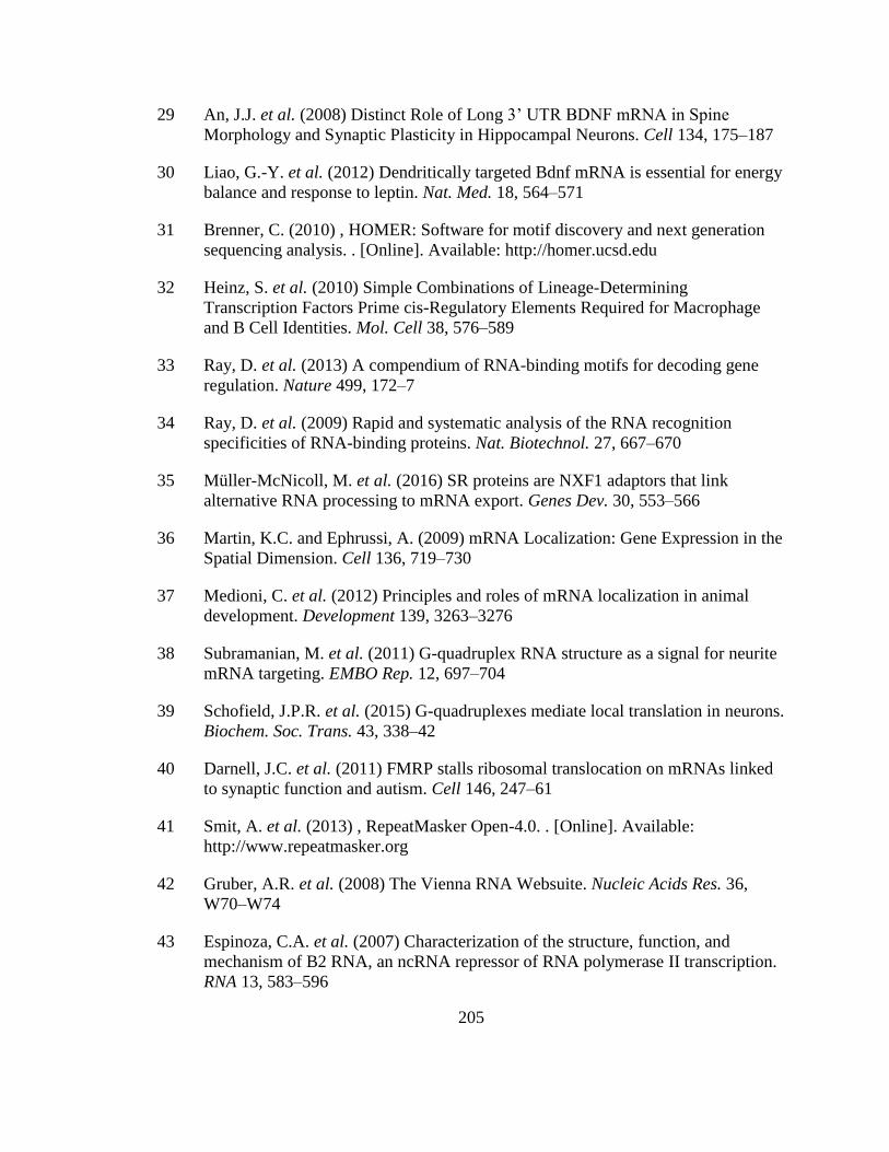
205
29 An, J.J. et al. (2008) Distinct Role of Long 3’ UTR BDNF mRNA in Spine
Morphology and Synaptic Plasticity in Hippocampal Neurons. Cell 134, 175–187
30 Liao, G.-Y. et al. (2012) Dendritically targeted Bdnf mRNA is essential for energy
balance and response to leptin. Nat. Med. 18, 564–571
31 Brenner, C. (2010) , HOMER: Software for motif discovery and next generation
sequencing analysis. . [Online]. Available: http://homer.ucsd.edu
32 Heinz, S. et al. (2010) Simple Combinations of Lineage-Determining
Transcription Factors Prime cis-Regulatory Elements Required for Macrophage
and B Cell Identities. Mol. Cell 38, 576–589
33 Ray, D. et al. (2013) A compendium of RNA-binding motifs for decoding gene
regulation. Nature 499, 172–7
34 Ray, D. et al. (2009) Rapid and systematic analysis of the RNA recognition
specificities of RNA-binding proteins. Nat. Biotechnol. 27, 667–670
35 Müller-McNicoll, M. et al. (2016) SR proteins are NXF1 adaptors that link
alternative RNA processing to mRNA export. Genes Dev. 30, 553–566
36 Martin, K.C. and Ephrussi, A. (2009) mRNA Localization: Gene Expression in the
Spatial Dimension. Cell 136, 719–730
37 Medioni, C. et al. (2012) Principles and roles of mRNA localization in animal
development. Development 139, 3263–3276
38 Subramanian, M. et al. (2011) G-quadruplex RNA structure as a signal for neurite
mRNA targeting. EMBO Rep. 12, 697–704
39 Schofield, J.P.R. et al. (2015) G-quadruplexes mediate local translation in neurons.
Biochem. Soc. Trans. 43, 338–42
40 Darnell, J.C. et al. (2011) FMRP stalls ribosomal translocation on mRNAs linked
to synaptic function and autism. Cell 146, 247–61
41 Smit, A. et al. (2013) , RepeatMasker Open-4.0. . [Online]. Available:
http://www.repeatmasker.org
42 Gruber, A.R. et al. (2008) The Vienna RNA Websuite. Nucleic Acids Res. 36,
W70–W74
43 Espinoza, C.A. et al. (2007) Characterization of the structure, function, and
mechanism of B2 RNA, an ncRNA repressor of RNA polymerase II transcription.
RNA 13, 583–596
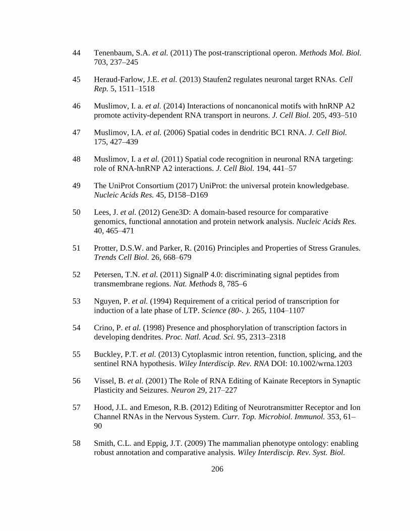
206
44 Tenenbaum, S.A. et al. (2011) The post-transcriptional operon. Methods Mol. Biol.
703, 237–245
45 Heraud-Farlow, J.E. et al. (2013) Staufen2 regulates neuronal target RNAs. Cell
Rep. 5, 1511–1518
46 Muslimov, I. a. et al. (2014) Interactions of noncanonical motifs with hnRNP A2
promote activity-dependent RNA transport in neurons. J. Cell Biol. 205, 493–510
47 Muslimov, I.A. et al. (2006) Spatial codes in dendritic BC1 RNA. J. Cell Biol.
175, 427–439
48 Muslimov, I. a et al. (2011) Spatial code recognition in neuronal RNA targeting:
role of RNA-hnRNP A2 interactions. J. Cell Biol. 194, 441–57
49 The UniProt Consortium (2017) UniProt: the universal protein knowledgebase.
Nucleic Acids Res. 45, D158–D169
50 Lees, J. et al. (2012) Gene3D: A domain-based resource for comparative
genomics, functional annotation and protein network analysis. Nucleic Acids Res.
40, 465–471
51 Protter, D.S.W. and Parker, R. (2016) Principles and Properties of Stress Granules.
Trends Cell Biol. 26, 668–679
52 Petersen, T.N. et al. (2011) SignalP 4.0: discriminating signal peptides from
transmembrane regions. Nat. Methods 8, 785–6
53 Nguyen, P. et al. (1994) Requirement of a critical period of transcription for
induction of a late phase of LTP. Science (80-. ). 265, 1104–1107
54 Crino, P. et al. (1998) Presence and phosphorylation of transcription factors in
developing dendrites. Proc. Natl. Acad. Sci. 95, 2313–2318
55 Buckley, P.T. et al. (2013) Cytoplasmic intron retention, function, splicing, and the
sentinel RNA hypothesis. Wiley Interdiscip. Rev. RNA DOI: 10.1002/wrna.1203
56 Vissel, B. et al. (2001) The Role of RNA Editing of Kainate Receptors in Synaptic
Plasticity and Seizures. Neuron 29, 217–227
57 Hood, J.L. and Emeson, R.B. (2012) Editing of Neurotransmitter Receptor and Ion
Channel RNAs in the Nervous System. Curr. Top. Microbiol. Immunol. 353, 61–
90
58 Smith, C.L. and Eppig, J.T. (2009) The mammalian phenotype ontology: enabling
robust annotation and comparative analysis. Wiley Interdiscip. Rev. Syst. Biol.
207
Med. 1, 390–399
59 Adzhubei, I.A. et al. (2010) A method and server for predicting damaging
missense mutations. Nat. Methods 7, 248–249
60 Tongiorgi, E. et al. (1997) Activity-dependent dendritic targeting of BDNF and
TrkB mRNAs in hippocampal neurons. J. Neurosci. 17, 9492–9505
61 Steward, O. et al. (1998) Synaptic activation causes the mRNA for the IEG Arc to
localize selectively near activated postsynaptic sites on dendrites. Neuron 21, 741–
751
62 Eberwine, J. et al. (2001) Local translation of classes of mRNAs that are targeted
to neuronal dendrites. Proc. Natl. Acad. Sci. 98, 7080–7085
63 Yoon, Y.J. et al. (2016) Glutamate-induced RNA localization and translation in
neurons. Proc. Natl. Acad. Sci. 113, E6877–E6886
64 Buchhalter, J.R. and Dichter, M.A. (1991) Electrophysiological comparison of
pyramidal and stellate nonpyramidal neurons in dissociated cell culture of rat
hippocampus. Brain Res. Bull. 26, 333–338
65 Morris, J. et al. (2011) Transcriptome analysis of single cells. J. Vis. Exp. DOI:
10.3791/2634
66 Dobin, A. et al. (2013) STAR: ultrafast universal RNA-seq aligner. Bioinformatics
29, 15–21
67 Zhu, Q. et al. (2016) VERSE: a versatile and efficient RNA-Seq read counting
tool. bioRxiv DOI: https://doi.org/10.1101/053306
68 Zhang, Y. et al. (2014) An RNA-Sequencing Transcriptome and Splicing Database
of Glia, Neurons, and Vascular Cells of the Cerebral Cortex. J. Neurosci. 34,
11929–11947
69 Eden, E. et al. (2009) GOrilla: a tool for discovery and visualization of enriched
GO terms in ranked gene lists. BMC Bioinformatics 10, 48
70 Middleton, S.A. and Kim, J. (2014) NoFold: RNA structure clustering without
folding or alignment. RNA 20, 1671–1683
71 Yeats, C. et al. (2010) A fast and automated solution for accurately resolving
protein domain architectures. Bioinformatics 26, 745–751
72 Landrum, M.J. et al. (2016) ClinVar: public archive of interpretations of clinically
relevant variants. Nucleic Acids Res. 44, D862–D868
208
73 Kerpedjiev, P. et al. (2015) Forna (force-directed RNA): Simple and effective
online RNA secondary structure diagrams. Bioinformatics 31, 3377–3379
74 Lai, D. et al. (2012) R-CHIE: a web server and R package for visualizing RNA
secondary structures. Nucleic Acids Res. 40, e95–e95

209
Chapter 5: Conclusions and future directions
The incorporation of structure information into routine bioinformatics analysis
has been hindered by a lack of tools that can analyze structure on a large scale. In this
thesis, I described two novel methods for characterizing macromolecular structure that
utilize the idea of empirical feature spaces to improve accuracy and scalability. I then
applied these methods to address long-standing open questions in neuron biology
regarding localization and translation in the dendrites, which has significance for our
understanding of long-term potentiation and learning and memory. These results include
findings that would have been more difficult to obtain without structure analysis,
including the identification of B1 and B2-derived hairpin structures in localized 3’UTRs,
and new predictions RBPs and RNA binding domains (RBDs) among locally-translated
proteins. Altogether, this work demonstrates the utility of structure-based analysis of
macromolecules and provides two scalable methods to implement such analyses in
standard bioinformatics pipelines. In the discussion below, I highlight some important
avenues for follow-up work, including areas where structure-based analysis of RNA and
protein could be particularly fruitful.

210
Role of alternative 3’UTRs in RNA localization
Neurons clearly have special RNA localization needs compared to other cell
types. Their unique morphology—long, extended processes that can be many times the
length of the soma—combined with an extensive need for local translation means that
neurons must transport a wide variety of RNAs long distances from their origination
point in the nucleus. In Chapter 4, we found almost 300 genes with alternative 3’
isoforms where one isoform was consistently more dendritically localized than the other.
There are several reasons why the use of alternative 3’UTRs is an attractive model for
how neurons might regulate localization. Firstly, it provides the neuron with a mechanism
for localizing only a subset of the transcripts of a given gene. This is potentially critical
for any genes where the RNA and/or protein is needed in the soma in addition to the
dendrites. Secondly, localizing only a subset of gene isoforms allows neurons to
potentially regulate the localization of RNAs using co-transcriptional mechanisms, such
as controlling the level of splicing factors that promote inclusion/exclusion of the
localized isoform. Finally, alternative 3’UTRs theoretically have the potential to provide
an element of tissue-specificity to localization, since cell types that have no need to
localize a particular RNA can simply not express the localized isoform. However, in
contrast to this idea, we did not observe a high level of tissue-specificity among the
neurite-targeted 3’ isoforms. Specifically, of the 38 neurite-targeted isoforms we
identified that were among the new 3’UTRs annotated by Miura et al. [1], only 12 were
specific to hippocampal neurons according to the Miura data. The other 26 isoforms were
found in at least one of the other mouse tissue types profiling in that study, which

211
included spleen, liver, thymus, lung, and heart [1]. This suggests that regulation of
alternative 3’UTR usage may not be the main mechanism of generating tissue-specific
localization. Another way that tissue-specific localization might be achieved is through
the regulated expression of the trans factors needed for localization, e.g. certain RBPs or
transport components. Overall, more work is needed to determine how differentially
localized 3’ isoforms are regulated in neurons. It will be interesting to see if any other
structural motifs can be found in the RNAs that might play a role in regulating splicing
patterns, such that a neuron can trigger the inclusion or exclusion of DTE-containing 3’
exons, depending on its localization needs.
RBPs in dendritic localization
Although we focused our attention here on identifying the cis elements involved
in dendritic localization—i.e. linear and structural DTEs found on the RNA itself—the
RBP trans factors that bind these elements are likely to be just as important for a full
understanding of RNA localization. RBPs appear to be hotspots for mutations associated
with neuropsychiatric disorders [2,3], including several with putative roles in
localization, suggesting that errors in RNA localization could be major mechanism
underlying disease. A more complete understanding of the interactions between
localization-mediating RBPs and the DTEs they bind is therefore needed. Several
experimental methods are now being used to profile these interactions transcriptome-
wide, such as crosslinking immunoprecipitation (CLIP)-based methods to identify the
RNAs bound by specific RBPs [4–6], peptide nucleic acid (PNA)-assisted identification

212
of RBPs (PAIR) to identify the RBPs associated with a specific RNAs [7], as well as
methods that profile protein-bound RNA more broadly [8]. Although these methods
reveal which RNAs are RBP-bound and sometimes even the location of the binding sites,
they usually only provide limited information about the motifs recognized by the RBP.
Often only a short, degenerate linear motif is identified (e.g. “YGCY” for Mbnl1 [9] and
“UCAY” for Nova [10]). More sophisticated tools for determining binding motifs that
incorporate both sequence and structure will need to be applied to fully capture the
binding preferences of RBPs (this will be discussed further below). In order to make
useful predictions about mutations that could disrupt the interaction between localization-
mediating RBPs and their targets, we will need more accurate models of the structure of
both the RBP binding domain(s) and the RNA binding site. In addition, a more complete
definition of which RBPs are involved in localization will help focus such studies.
Neo-functionalization of transposable elements
The results of the RNA structure motif analysis in Chapter 4 suggested that B1
and B2 SINE elements could play a role in localization in mouse neurons. Such neo-
functionalizations of transposable elements have been described previously in several
other contexts, and are hypothesized to be one of the major sources of new functional
genomic elements [11–15]. In particular, as mentioned previously, it had been shown that
another type of SINE called the ID element—derived from the dendritically-localized
ncRNA BC1—caused localization of RNAs to the dendrites in rat [16–18]. Interestingly,
however, this localization was not reproduced in mice [19,20], suggesting that it could be
213
a rat-specific innovation. Supporting this hypothesis is the fact that ID elements have
undergone greater expansion in rat compared to mouse, with over 100x more instances in
rat [17]. In the same study, it was found that B2 elements did not cause dendritic
localization in rat [17]. Localization ability of B1 and B2 elements have not yet been
experimentally tested in mouse, but given the divergence of functionality observed for ID
elements between rodents, a similar divergence for B1 and/or B2 elements should not be
ruled out. The possibility of analogous, yet non-homologous elements performing similar
roles in different species has been noted before, both for transposons and non-transposon
motifs [14,21]. Therefore, it is worth investigating whether a similar analogous-but-not-
homologous relationship exists for ID elements and B1/B2 elements in the context of
dendritic localization.
If B1/B2 elements drive dendritic localization in mice and ID elements drive
localization in rats, what element might fill this role in humans? Several lines of evidence
point to Alu elements being a likely candidate. Alu elements are primate-specific SINE
retrotransposons that make up almost 11% of the human genome [22]. They are
originally derived from 7SL RNA, which is part of the signal recognition RNP and plays
a role in the processing and localization of proteins with signal peptides. In humans, Alu
elements show “exonization” activity, where an Alu element within an intron becomes an
exon via activation of the cryptic splice sites contained in the Alu sequence [22]. Relevant
to our previous discussion of the role of alternative 3’UTRs in localization, it has also
been found that Alu elements located downstream of a gene can generate new alternative
3’UTRs by alternative splicing or alternative cleavage and polyadenylation, and
214
furthermore, that these Alu-derived 3’UTRs tend to be tissue specific [15]. Most notably
of all, a potential role for an Alu-derived element in dendritic localization has already
been described: BC200, a ncRNA that likely originated from an Alu element, shows
dendritic localization patterns highly similar to BC1 RNA in rodents [23]. Since no
homolog of BC1 has been found in humans, BC200 is often described as the primate
“analog” of BC1. Alu elements appear to fill analogous roles for other types of rodent
SINEs as well, including mouse B2 SINE RNA in repression of Pol II during heat shock
[24]. Overall, there appear to be many points of convergence between these different
classes of SINE elements in mouse, rat, and human, despite their distinct evolutionary
origins and extensive species-specific expansions and insertions. Further exploration of
the potential role of Alu elements in human dendritic localization will be an important
area for future work.
Function of locally translated proteins in L-LTP
A crucial remaining question is what role individual locally translated proteins
play in long-lasting synaptic potentiation. Part of the difficulty of answering this question
is the need to ensure that any method used to block the translation of an RNA is specific
to the RNA in question and only affects RNA in the dendrites—the somatic translation
should be left intact. For CaMKIIα, this was accomplished by deleting the region of the
3’UTR that contained the DTE, thus blocking local translation via abolishing
localization. With better definition of DTEs, it will become possible to perform this sort
215
of analysis across more RNAs and with greater specificity—i.e. removing only the DTE
rather than large regions of the 3’UTR.
Another interesting question is when proteins are locally translated. Are certain
subsets translated constitutively? How long after synaptic activation does local translation
of different RNAs occur? Is there any sequential order to the translation of different
RNAs after synaptic activation? Methods that monitor translation in real time with spatial
precision will be helpful to answer these questions [25,26]. Real-time translation data has
been reported for a handful of specific RNAs so far [27–31], and it will be particularly
interesting to see local translation profiled on a larger scale.
Beyond neurons: other applications of structure analysis
Macromolecular structure plays an important role in all tissues and cellular
pathways, and thus there is no shortage of areas where large-scale structure-based
analysis can shed new light. For mRNAs, any co-regulated group of transcripts likely
shares a common motif that is recognized by the regulating RBP, and many of these
motifs are likely to have structural characteristics. Structure-aware de novo motif finding
tools such as NoFold can be applied to these transcripts to identify binding motifs.
Examples could include identification of structure motifs in the 3’UTR that increase or
decrease mRNA stability, structures that promote exon inclusion or exclusion, or
structures that enhance or repress translation.
For proteins, fast and sensitive methods for predicting tertiary structure from
amino acid sequence will continue to be of vital importance as the number of protein
216
sequences in databases grows. Although some structural folds are relatively easy to
identify using linear information (e.g. HMM-based methods like Gene3D and Pfam),
other folds are so diverse on the sequence level that they can sometimes only be
identified using higher-order structure information (e.g. threading-based methods). An
example of this is the Piwi domain—an RNA endonuclease structure found in the PIWI
and Argonaut families of proteins, among others. The Piwi domain has a conserved
structure, but the sequences that form this structure are highly diverse [32,33] (see also
the CATH entry for this structure: [34]), making it difficult to identify based on sequence
alone. Structural feature spaces such as the PESS are well suited for classification tasks
such as this. The PESS can also be used as a rapid structure-based query system, as
demonstrated with the hedgehog-related proteins in Chapter 3. In this framework, a
whole proteome that has already been mapped to the PESS can be quickly queried for the
closest structural matches to a domain of interest. Although the initial set up of the
whole-proteome database is time consuming (requiring threading all domains in the
proteome against the 1,814 templates, as described in Chapter 3), this step only needs to
be performed once. Thereafter, all “queries” to the database require only threading of the
query, and then a rapid nearest neighbor-based search of the PESS to retrieve the closest
matches. We have already created PESS databases for the human and C. elegans
proteomes, as well as a large portion of the mouse proteome (neuronally-expressed
genes), and so queries to these proteomes are already possible.
Remaining challenges for structure prediction
217
The ability to predict the RNA motifs bound by RBPs with high accuracy is a
major area of future improvement. An ideal method would include primary, secondary,
and tertiary structure information, since all of these levels can be important for
determining the affinity of an RBP for a particular RNA. Furthermore, future methods
need to more fully take into account the way in which RBPs bind. Typically, an RBP
contains multiple RBDs, each of which bind relatively weakly to their target motifs, and
it is the combination of multiple bound RBDs that give an RBP its specificity and
strengthens the interaction with the RNA [35]. For example, RNA recognition motif
(RRM) RBDs typically recognize only 4-8nt, often with some degree of ambiguity of the
exact recognition motif [36]. In order to gain greater specificity, most RBPs with RRM
domains contain multiple such domains [35]. The implication is that in order to fully
characterize the binding preferences of an RBP, one must look for multiple motifs. To
make matters even more complicated, it is likely that the space between the motifs on the
RNA is also important for recognition. The particular spacing needed will depend on the
relative orientation and flexibility of the RBDs within the RBP: if two RBDs have a
relatively short linker sequence between them, they may be fairly rigid and require a very
specific distance between the two RNA motifs for binding; on the other hand, if two
RBDs have a long, flexible linker between them, they could be more tolerant to the
spacing between the RNA motifs. RNA structure and flexibility may also need to be
taken into account. As a final layer of complexity, there are many cases where structural
conformations change during binding. In this type of binding, called “induced fit”, the
RNA or RBP (or both) starts off in one conformation—typically a flexible or disordered
218
state—and then changes in structure upon binding [37]. An example of this is the
“zipcode” RNA motif and its RBP partner, ZBP1, which are involved in dendritic
localization of β-actin RNA. Initially, the region of the β-actin RNA that contains the
zipcode sequence exists in an unfolded state, but then takes on more stable secondary
structure by looping around ZBP1 [38]. Altogether, the interactions between RNA and
RBPs are clearly complex and will require sophisticated tools to predict with accuracy in
a reasonable amount of time. In the meantime, methods that aid in predicting secondary
structure motifs of RNA and tertiary structural folds of RBPs bring us a step closer to a
complete picture.
In terms of protein structure prediction, one of the greatest challenges still
remaining is accurate prediction of domain boundaries based on protein sequence.
Segmenting a protein into domains is the first step of many protein structure prediction
methods, and is particularly crucial (and particularly difficult) when there is little
sequence similarity between the query and any structurally solved protein. Improper
domain segmentation was one of the major sources of low-confidence predictions in our
classification of the human proteome (Chapter 3). Improvements in this area will be key
for higher quality predictions downstream.
Conclusion
Macromolecules can only be fully understood if they are considered in the context
of both their sequence and structural characteristics. In this thesis, I have demonstrated
several ways that computational structure analysis can lead to new insights and make
219
testable predictions, and more generally help make sense of the huge amount of sequence
data that is now commonplace in genomics experiments. There are still many
improvements that can be made, and experimental follow up will often be needed to
verify predictions. Nonetheless, there is little doubt that structure analysis tools that can
handle large-scale datasets will be instrumental to the field of genomics as it continues to
mature.

220
References
1 Miura, P. et al. (2013) Widespread and extensive lengthening of 3’ UTRs in the
mammalian brain. Genome Res. 23, 812–25
2 Liu-Yesucevitz, L. et al. (2011) Local RNA translation at the synapse and in
disease. J. Neurosci. 31, 16086–93
3 Nussbacher, J.K. et al. (2015) RNA-binding proteins in neurodegeneration: Seq
and you shall receive. Trends Neurosci. DOI: 10.1016/j.tins.2015.02.003
4 Ule, J. et al. (2003) CLIP identifies Nova-regulated RNA networks in the brain.
Science 302, 1212–5
5 Licatalosi, D.D. et al. (2008) HITS-CLIP yields genome-wide insights into brain
alternative RNA processing. Nature 456, 464–9
6 Hafner, M. et al. (2010) Transcriptome-wide identification of RNA-binding
protein and microRNA target sites by PAR-CLIP. Cell 141, 129–41
7 Zielinski, J. et al. (2006) In vivo identification of ribonucleoprotein-RNA
interactions. Proc. Natl. Acad. Sci. U. S. A. 103, 1557–62
8 Silverman, I.M. et al. (2014) RNase-mediated protein footprint sequencing reveals
protein-binding sites throughout the human transcriptome. Genome Biol. 15, R3
9 Goers, E.S. et al. (2010) MBNL1 binds GC motifs embedded in pyrimidines to
regulate alternative splicing. Nucleic Acids Res. 38, 2467–2484
10 Jensen, K.B. et al. (2000) The tetranucleotide UCAY directs the specific
recognition of RNA by the Nova K-homology 3 domain. Proc. Natl. Acad. Sci. U.
S. A. 97, 5740–5
11 McDonald, J.F. (1995) Transposable elements: possible catalysts of organismic
evolution. Trends Ecol. Evol. 10, 123–126
12 Brosius, J. (1999) RNAs from all categories generate retrosequences that may be
exapted as novel genes or regulatory elements. Gene 238, 115–134
13 Jordan, I.K. et al. (2003) Origin of a substantial fraction of human regulatory
sequences from transposable elements. Trends Genet. 19, 68–72
14 G, B. et al. (2008) Evolution of the mammalian transcription factor binding
repertoire via transposable elements. DOI: 10.1101/gr.080663.108.These
221
15 Tajnik, M. et al. (2015) Intergenic Alu exonisation facilitates the evolution of
tissue-specific transcript ends. Nucleic Acids Res. 43, gkv956
16 Muslimov, I.A. et al. (2006) Spatial codes in dendritic BC1 RNA. J. Cell Biol.
175, 427–439
17 Buckley, P.T. et al. (2011) Cytoplasmic intron sequence-retaining transcripts can
be dendritically targeted via ID element retrotransposons. Neuron 69, 877–84
18 Muslimov, I. a. et al. (2014) Interactions of noncanonical motifs with hnRNP A2
promote activity-dependent RNA transport in neurons. J. Cell Biol. 205, 493–510
19 Khanam, T. et al. (2007) Can ID repetitive elements serve as cis-acting dendritic
targeting elements? An in vivo study. PLoS One 2, e961
20 Robeck, T. et al. (2016) BC1 RNA motifs required for dendritic transport in vivo.
Sci. Rep. 6, 28300
21 Tsirigos, A. and Rigoutsos, I. (2008) Human and mouse introns are linked to the
same processes and functions through each genome’s most frequent non-conserved
motifs. Nucleic Acids Res. 36, 3484–3493
22 Deininger, P. et al. (2011) Alu elements: know the SINEs. Genome Biol. 12, 236
23 Tiedge, H. et al. (1993) Primary structure, neural-specific expression, and
dendritic location of human BC200 RNA. J. Neurosci. 13, 2382–2390
24 Espinoza, C.A. et al. (2007) Characterization of the structure, function, and
mechanism of B2 RNA, an ncRNA repressor of RNA polymerase II transcription.
RNA 13, 583–596
25 Wu, B. et al. (2016) Translation dynamics of single mRNAs in live cells and
neurons. Science (80-. ). 1084,
26 Morisaki, T. et al. (2016) Real-time quantification of single RNA translation
dynamics in living cells. Science (80-. ). 899, 1–10
27 Aakalu, G. et al. (2001) Dynamic visualization of local protein synthesis in
hippocampal neurons. Neuron 30, 489–502
28 Raab-Graham, K.F. et al. (2006) Activity- and mTOR-Dependent Suppression of
Kv1.1 Channel mRNA Translation in Dendrites. Science (80-. ). 314, 144–148
29 Wang, D.O. et al. (2009) Synapse- and stimulus-specific local translation during
long-term neuronal plasticity. Science 324, 1536–40
222
30 Swanger, S.A. et al. (2013) Dendritic GluN2A Synthesis Mediates Activity-
Induced NMDA Receptor Insertion. J. Neurosci. 33, 8898–8908
31 Kim, T.K. et al. (2013) Dendritic glutamate receptor mRNAs show contingent
local hotspot-dependent translational dynamics. Cell Rep. 5, 114–25
32 Burroughs, A.M. et al. (2013) Two novel PIWI families: roles in inter-genomic
conflicts in bacteria and Mediator-dependent modulation of transcription in
eukaryotes. Biol. Direct 8, 13
33 Swarts, D.C. et al. (2014) The evolutionary journey of Argonaute proteins. Nat
Struct Mol Biol 21, 743–753
34 CATH CATH Superfamily 3.40.50.2300. . [Online]. Available:
http://www.cathdb.info/version/v4_1_0/superfamily/3.40.50.2300
35 Lunde, B.M. et al. (2007) RNA-binding proteins: modular design for efficient
function. Nat. Rev. Mol. Cell Biol. 8, 479–90
36 Maris, C. et al. (2005) The RNA recognition motif, a plastic RNA-binding
platform to regulate post-transcriptional gene expression. FEBS J. 272, 2118–2131
37 Williamson, J.R. (2000) Induced fit in RNA-protein recognition. Nat. Struct. Biol.
7, 834–837
38 Patel, V.L. et al. (2012) Spatial arrangement of an RNA zipcode identifies mRNAs
under post-transcriptional control. Genes Dev. 26, 43–53