structural scene analysis of remotely sensed images using graph …ozdemir/papers/ms_thesis.pdf ·...
TRANSCRIPT

STRUCTURAL SCENE ANALYSIS OFREMOTELY SENSED IMAGES USING
GRAPH MINING
a thesis
submitted to the department of computer engineering
and the institute of engineering and science
of bilkent university
in partial fulfillment of the requirements
for the degree of
master of science
By
Bahadır Ozdemir
July, 2010

I certify that I have read this thesis and that in my opinion it is fully adequate,
in scope and in quality, as a thesis for the degree of Master of Science.
Assist. Prof. Dr. Selim Aksoy (Advisor)
I certify that I have read this thesis and that in my opinion it is fully adequate,
in scope and in quality, as a thesis for the degree of Master of Science.
Assist. Prof. Dr. Cigdem Gunduz Demir
I certify that I have read this thesis and that in my opinion it is fully adequate,
in scope and in quality, as a thesis for the degree of Master of Science.
Assist. Prof. Dr. Tolga Can
Approved for the Institute of Engineering and Science:
Prof. Dr. Levent OnuralDirector of the Institute
ii
ABSTRACT
STRUCTURAL SCENE ANALYSIS OF REMOTELYSENSED IMAGES USING GRAPH MINING
Bahadır Ozdemir
M.S. in Computer Engineering
Supervisor: Assist. Prof. Dr. Selim Aksoy
July, 2010
The need for intelligent systems capable of automatic content extraction and
classification in remote sensing image datasets, has been constantly increasing
due to the advances in the satellite technology and the availability of detailed
images with a wide coverage of the Earth. Increasing details in very high spatial
resolution images obtained from new generation sensors have enabled new ap-
plications but also introduced new challenges for object recognition. Contextual
information about the image structures has the potential of improving individual
object detection. Therefore, identifying the image regions which are intrinsically
heterogeneous is an alternative way for high-level understanding of the image
content. These regions, also known as compound structures, are comprised of
primitive objects of many diverse types. Popular representations such as the
bag-of-words model use primitive object parts extracted using local operators but
cannot capture their structure because of the lack of spatial information. Hence,
the detection of compound structures necessitates new image representations that
involve joint modeling of spectral, spatial and structural information.
We propose an image representation that combines the representational power
of graphs with the efficiency of the bag-of-words representation. The proposed
method has three parts. In the first part, every image in the dataset is trans-
formed into a graph structure using the local image features and their spatial
relationships. The transformation method first detects the local patches of inter-
est using maximally stable extremal regions obtained by gray level thresholding.
Next, these patches are quantized to form a codebook of local information and a
graph is constructed for each image by representing the patches as the graph nodes
and connecting them with edges obtained using Voronoi tessellations. Transform-
ing images to graphs provides an abstraction level and the remaining operations
iii

iv
for the classification are made on graphs. The second part of the proposed method
is a graph mining algorithm which finds a set of most important subgraphs for the
classification of image graphs. The graph mining algorithm we propose first finds
the frequent subgraphs for each class, then selects the most discriminative ones
by quantifying the correlations between the subgraphs and the classes in terms of
the within-class occurrence distributions of the subgraphs; and finally reduces the
set size by selecting the most representative ones by considering the redundancy
between the subgraphs. After mining the set of subgraphs, each image graph
is represented by a histogram vector of this set where each component in the
histogram stores the number of occurrences of a particular subgraph in the im-
age. The subgraph histogram representation enables classifying the image graphs
using statistical classifiers. The last part of the method involves model learning
from labeled data. We use support vector machines (SVM) for classifying images
into semantic scene types. In addition, the themes distributed among the im-
ages are discovered using the latent Dirichlet allocation (LDA) model trained on
the same data. By this way, the images which have heterogeneous content from
different scene types can be represented in terms of a theme distribution vector.
This representation enables further classification of images by theme analysis.
The experiments using an Ikonos image of Antalya show the effectiveness of
the proposed representation in classification of complex scene types. The SVM
model achieved a promising classification accuracy on the images cut from the
Antalya image for the eight high-level semantic classes. Furthermore, the LDA
model discovered interesting themes in the whole satellite image.
Keywords: Graph-based scene analysis, graph mining, scene understanding, re-
mote sensing image analysis.

OZET
UYDU GORUNTULERININ CIZGE MADENCILIGI ILEYAPISAL SAHNE ANALIZI
Bahadır Ozdemir
Bilgisayar Muhendisligi, Yuksek Lisans
Tez Yoneticisi: Y. Doc. Dr. Selim Aksoy
Temmuz, 2010
Uydu teknolojisindeki gelismeler ve Dunya’nın genis bir yuzeyini kapsayan
detaylı goruntulerin mevcut olması, uydu goruntulerinde otomatik icerik cıkarma
ve sınıflandırma yapabilen akıllı sistemlere duyulan ihtiyacı her gecen gun
arttırmaktadır. Yeni nesil sensorlerden alınan cok yuksek uzamsal cozunurluklu
goruntulerdeki artan detaylar yeni uygulamaları mumkun kılmakla birlikte temel
nesnelerin sezimini zorlastırmaktadır. Goruntu yapıları hakkındaki baglamsal
bilgiler birbirinden bagımsız nesnelerin sezimini gelistirme potansiyeline sahiptir.
Bu nedenle, ozunde heterojen olan goruntu bolgelerinin tanımlanması, goruntu
icerigini anlamak icin alternatif bir yoldur. Bilesik yapılar olarak da bilinen
bu bolgeler bircok farklı turdeki temel nesnelerden olusmaktadır. Kelimeler-
torbası gibi populer gosterimler, yerel operatorler kullanılarak cıkarılan temel
nesne parcalarını kullanır fakat mekansal bilgi eksikligi nedeniyle onların yapısını
tutamaz. Dolayısıyla, bilesik yapıların sezimi spektral, uzaysal ve yapısal bilgi-
lerin ortak modellenmesini iceren yeni goruntu gosterimlerini zorunlu kılar.
Biz, cizgelerin gosterim gucu ile kelimeler-torbası gosteriminin verimliligini
birlestiren bir goruntu gosterimi oneriyoruz. Onerilen yontem uc bolumden
olusmaktadır. Ilk bolumde, veri kumesindeki her bir goruntu yerel goruntu
ozellikleri ve onların uzamsal iliskileri kullanılarak cizge yapısına donusturulur.
Donusturme yontemi ilk olarak gri seviye esiklemesi ile elde edilen en kararlı uc
bolgelerden, ilgili yerel yamaları tespit eder. Sonra, bu yamalar bir yerel bilgi
cizelgesi olusturmak icin nicelendirilir, ve yamaları cizge dugumu gibi gostererek
ve onları Voronoi mozaiginden elde edilen kenarlarla birlestirerek her bir goruntu
icin bir cizge insa edilir. Goruntulerin cizgelere donusturulmesi bir soyut-
lama duzeyi saglar ve sınıflandırma icin geriye kalan islemler cizgeler uzerinde
yapılır. Onerilen yontemin ikinci bolumu goruntu cizgelerinin sınıflandırılması
v

vi
icin en onemli altcizgelerin kumesini secen bir cizge madenciligi algorit-
masıdır. Onerdigimiz cizge madenciligi algoritması ilk olarak her sınıf icin
sık gorulen altcizgeleri bulur, sonra sınıf icinde gorulme dagılımları acısından
altcizgeler ve sınıflar arasındaki bagıntı miktarları olculerek en ayırt edici olan-
ları secer; ve son olarak altcizgeler arasındaki fazlalıgı dikkate alarak en iyi
temsil edenlerin secmesiyle kume boyutunu kucultur. Altcizge kumesi maden-
ciliginden sonra her bir goruntu cizgesi, her bir bileseninin bu kumenin belli
bir altcizgesinin goruntude gorulme sayısını tuttugu bir histogram vektoru
ile gosterilir. Altcizge histogram gosterimi goruntu cizgelerinin istatistiksel
sınıflandırıcılar kullanılarak sınıflandırılmasını mumkun kılar. Yontemin son
bolumu etiketli verilerinden model ogrenilmesini icerir. Goruntulerin anlam-
sal sahne turlerine sınıflandırılması icin destek vektor makineleri (DVM) kul-
lanıyoruz. Ek olarak, goruntuler uzerine dagılan temalar, aynı veriler uzerinde
ogretilen gizli Dirichlet tahsisi (GDT) modeli kullanılarak kesfedilir. Bu sayede,
farklı sahne turlerinden heterojen bir icerige sahip goruntuler bir tema dagılım
vektoru olarak gosterilebilirler. Bu gosterim tema analizi ile goruntulerin daha
ileri duzeyde sınıflandırılmasını saglar.
Antalya’nın bir Ikonos goruntusu uzerindeki deneyler onerilen gosterimin
karmasık sahne turlerinin sınıflandırılmasındaki etkinligini gostermektedir. DVM
modeli Antalya goruntusunden kesilen goruntulerde sekiz ust duzey anlamsal sınıf
icin umut verici sınıflandırma dogrulugu elde etti. Ayrıca, GDT modeli tum uydu
goruntusunde ilginc temalar kesfetti.
Anahtar sozcukler : Cizge tabanlı sahne analizi, cizge madenciligi, sahne anlayısı,
uydu goruntusu analizi.

Acknowledgement
I would like to express my sincere thanks to my advisor, Selim Aksoy, for his
guidance, suggestions and support throughout the development of this thesis. He
introduced me to the world of research, and encouraged me to develop my own
ideas for the problem while supporting each step with his knowledge and advice.
Whenever I got stuck in details, he provided me a different viewpoint. Working
with him has been a valuable experience for me.
I would like extend my thanks to the members of my thesis committee, Cigdem
Gunduz Demir and Tolga Can, for reviewing this thesis and their suggestions
about improving this work.
My special thanks must be sent to Fatos Tunay Yarman-Vural who introduced
me to computer vision when I was an undergraduate student at the Middle East
Technical University.
I would like to express my deepest gratitude to my family, always standing
by me, for their endless support and understanding.
I am very grateful to all those with whom I was having nice days in EA226:
Fırat, Daniya, Sare and Aslı. I am also grateful to Caglar and Gokhan for their
comments on the method and the scientific discussions.
Finally, I would like to thank TUBITAK BIDEB (The Scientific and Techno-
logical Research Council of Turkey) for their financial support during my master’s
studies. This work was also supported in part by the TUBITAK CAREER grant
104E074.
Bahadır Ozdemir
20 July 2010, Ankara
vii

Contents
1 Introduction 1
1.1 Overview . . . . . . . . . . . . . . . . . . . . . . . . . . . . . . . . 1
1.2 Problem Definition . . . . . . . . . . . . . . . . . . . . . . . . . . 2
1.3 Data Set . . . . . . . . . . . . . . . . . . . . . . . . . . . . . . . . 5
1.4 Summary of Contributions . . . . . . . . . . . . . . . . . . . . . . 6
1.5 Organization of the Thesis . . . . . . . . . . . . . . . . . . . . . . 9
2 Literature Review 10
2.1 Classification with Visual Words . . . . . . . . . . . . . . . . . . . 10
2.2 Classification with Graph Representation . . . . . . . . . . . . . . 11
3 Transforming Images to Graphs 14
3.1 Finding Regions of Interest . . . . . . . . . . . . . . . . . . . . . . 14
3.1.1 Maximally Stable Extremal Regions . . . . . . . . . . . . . 16
3.1.2 Types of Interest Regions . . . . . . . . . . . . . . . . . . 20
3.2 Feature Extraction . . . . . . . . . . . . . . . . . . . . . . . . . . 21
viii
CONTENTS ix
3.3 Graph Construction . . . . . . . . . . . . . . . . . . . . . . . . . . 27
3.3.1 Nodes and Labels . . . . . . . . . . . . . . . . . . . . . . . 27
3.3.2 Spatial Relationships and Edges . . . . . . . . . . . . . . . 28
4 Graph Mining 32
4.1 Foundations of Pattern Mining . . . . . . . . . . . . . . . . . . . 35
4.2 Frequent Pattern Mining . . . . . . . . . . . . . . . . . . . . . . . 36
4.3 Class Correlated Pattern Mining . . . . . . . . . . . . . . . . . . . 37
4.3.1 Mathematical Modeling of Pattern Support . . . . . . . . 38
4.3.2 Correlated Patterns . . . . . . . . . . . . . . . . . . . . . . 42
4.4 Redundancy-Aware Top-k Patterns . . . . . . . . . . . . . . . . . 52
4.5 Summary of the Mining Algorithm . . . . . . . . . . . . . . . . . 55
4.6 Graph Patterns . . . . . . . . . . . . . . . . . . . . . . . . . . . . 59
5 Scene Classification 64
5.1 Subgraph Histogram Representation . . . . . . . . . . . . . . . . 64
5.2 Support Vector Machines . . . . . . . . . . . . . . . . . . . . . . . 65
5.3 Latent Dirichlet Allocation . . . . . . . . . . . . . . . . . . . . . . 66
6 Experimental Results 71
6.1 Experimental Setup . . . . . . . . . . . . . . . . . . . . . . . . . . 71
6.1.1 Graph Construction Parameters . . . . . . . . . . . . . . . 72

CONTENTS x
6.1.2 Graph Mining Parameters . . . . . . . . . . . . . . . . . . 72
6.1.3 Classifier Parameters . . . . . . . . . . . . . . . . . . . . . 74
6.2 Classification Results . . . . . . . . . . . . . . . . . . . . . . . . . 74
7 Conclusions and Future Work 88
7.1 Conclusions . . . . . . . . . . . . . . . . . . . . . . . . . . . . . . 88
7.2 Future Work . . . . . . . . . . . . . . . . . . . . . . . . . . . . . . 90

List of Figures
1.1 Overall flowchart of the algorithm . . . . . . . . . . . . . . . . . . 4
1.2 An Ikonos image of Antalya, and some compound structures of in-
terest are zoomed in. The classes are (in clockwise order): Sparse
residential areas, orchards, greenhouses, fields, forests, dense res-
idential areas with small buildings, dense residential areas with
trees, and dense residential areas with large buildings. . . . . . . . 7
3.1 Steps of transforming images to graphs . . . . . . . . . . . . . . . 15
3.2 A given input image dark and bright MSERs, and ellipses fitted to
them for parameters Ω = (∆, a−, a+, v+, d+) = (10, 60, 5000, 0.4, 1). 19
3.3 Ellipses fitted to MSER groups stable dark, stable bright, unstable dark
and unstable bright are drawn with green, red, yellow and cyan,
respectively on different scene types for parameter sets Ωhigh =
(10, 60, 5000, 0.4, 1) and Ωlow = (5, 35, 1000, 4, 1). . . . . . . . 22
3.4 Satellite image of same region is given in (a) panchromatic and
(d) visible multispectral bands. In (b) and (e), a given MSER is
drawn with yellow and ellipse fitted to this MSER is drawn with
green. Expanded ellipses at squared Mahalanobis distance r21 = 5
and r22 = 20 are drawn with red and cyan, respectively. In (c) and
(f), pixels in Rin and Rout are shown for different bands. . . . . . 23
xi
LIST OF FIGURES xii
3.5 Results of morphological operations on images from three different
classes. Images from top to down are in the order: original images,
images closed by disk with radii 2, images closed by disk with radii
7, images opened by disk with radii 2 and images opened by disk
with radii 7. . . . . . . . . . . . . . . . . . . . . . . . . . . . . . . 25
3.6 A sample ellipse and its eigenvectors e1 and e2 are shown, corre-
sponding eigenvalues are λ1 and λ2, respectively. Major and minor
diameters are also shown. . . . . . . . . . . . . . . . . . . . . . . 26
3.7 The problem of discovering neighboring node pairs in the Voronoi
tessellation is shown in (a) and solution to this problem using ex-
ternal nodes is seen in (b). Corresponding graphs are given in (c)
and (d), respectively. . . . . . . . . . . . . . . . . . . . . . . . . . 30
3.8 Graph construction steps. The color and shape of a node in (d)
represent its label after k-means clustering. . . . . . . . . . . . . . 31
4.1 Steps of graph mining algorithm . . . . . . . . . . . . . . . . . . . 34
4.2 Poisson distributions with four different expected values. . . . . . 39
4.3 A sample histogram of a dataset with 100 elements and fitting
mixtures of 3 Poisson distributions to this histogram are shown in
blue and red, respectively. . . . . . . . . . . . . . . . . . . . . . . 42
4.4 The procedure for positive and negative distance computation is
illustrated for four classes. The interest class is the second one
and the distances are computed as p = EMD(P2, Pref) and n =
EMD(P3, Pref). . . . . . . . . . . . . . . . . . . . . . . . . . . . . . 47
4.5 The correlation function γ(p, n) . . . . . . . . . . . . . . . . . . . 48
4.6 Plot of a convex function f . . . . . . . . . . . . . . . . . . . . . . 51
4.7 Two sample redundant graph patterns . . . . . . . . . . . . . . . 53

LIST OF FIGURES xiii
4.8 The pn space showing the search regions for the first two steps
of the algorithm. The shaded area (union of dark and light gray)
represent the domain region of Fc and dark gray area represents
the domain region of Rc. . . . . . . . . . . . . . . . . . . . . . . . 58
4.9 An example for overlapping embeddings . . . . . . . . . . . . . . 60
4.10 In (a) The embeddings of the subgraph in Figure 4.9(a); in (b) the
corresponding overlap graph. . . . . . . . . . . . . . . . . . . . . . 62
4.11 Images from top to down are original images from three different
classes, image graphs for 36 labels, embeddings of sample sub-
graphs found by the mining algorithm and the sample subgraphs
where the color and shape of a node represents its label. . . . . . 63
5.1 Graphical model representation of LDA. The boxes are plates rep-
resenting replicates. The outer plate represents image graphs,
while the inner plate represents the repeated choice of themes and
subgraphs within an image graph [7]. . . . . . . . . . . . . . . . . 68
5.2 Graphical model representation of the variational distribution used
to approximate the posterior in LDA [7]. . . . . . . . . . . . . . . 69
6.1 Three clusters of stable dark MSERs are drawn with different col-
ors at ellipse centers forN` = 36. Yellow, green and magenta points
are concentrated on dense residential areas with large buildings,
dense residential areas with small buildings and orchards, respec-
tively. . . . . . . . . . . . . . . . . . . . . . . . . . . . . . . . . . 76
6.2 Four clusters of different type MSERs are drawn with different
colors at ellipse centers for N` = 36. Yellow, green, cyan and
magenta points are concentrated on sea, forests, stream bed/clouds
and dense residential areas with trees, respectively. . . . . . . . . 77

LIST OF FIGURES xiv
6.3 Plot of classification accuracy of the graph mining algorithm for
five different number of labels over the number of subgraphs per
class. The lines are drawn by averaging the accuracy values for the
parameters Nθ ∈ 200, 500, 800. . . . . . . . . . . . . . . . . . . . 79
6.4 Plot of classification accuracy of the graph mining algorithm for
three different Nθ values over the number of subgraphs per class.
The lines are drawn by averaging the accuracy values for the pa-
rameters N` ∈ 18, 26, 36, 54, 72. . . . . . . . . . . . . . . . . . . 81
6.5 The confusion matrix of the graph mining algorithm using the
parameters N` = 36, Nθ = 200 and Ns = 9. Class names are
given in short: sparse and dense are used for sparse and dense
residential areas, respectively. Also, large and small mean large
and small buildings, respectively. . . . . . . . . . . . . . . . . . . 83
6.6 The confusion matrix of the bag-of-words model for 26 labels.
Class names are given in short: sparse and dense are used for
sparse and dense residential areas, respectively. Also, large and
small mean large and small buildings, respectively. . . . . . . . . 83
6.7 Sample images from the dataset. The images at the left are
correctly classified by the graph mining algorithm while the im-
ages at right-hand side are misclassified using the parameters
N` = 36, Nθ = 200 and Ns = 9. The image classes from top
to down are in the order: dense residential areas with large build-
ings, dense residential areas with small buildings, dense residential
areas with trees, sparse residential areas, greenhouses, orchards,
forests and fields. . . . . . . . . . . . . . . . . . . . . . . . . . . . 84
6.8 The classification of all tiles except sea using the SVM learned
from the training set for the parameters N` = 36, Nθ = 200 and
Ns = 9. Each color represents a unique class. . . . . . . . . . . . . 85

LIST OF FIGURES xv
6.9 Every tile is labeled by a unique color which indicates the cor-
responding theme that dominates the other themes in that tile.
The theme distributions are inferred from the LDA model for 12
themes. The subgraph set is the one mined in the previous exper-
iments for the best parameters. . . . . . . . . . . . . . . . . . . . 86
6.10 The most dominating 6 themes are shown, found by the LDA
model trained for 16 themes. The intensity of red color represents
the probability of the theme in an individual tile. . . . . . . . . . 87

List of Tables
3.1 Ten basic features extracted from four bands and two regions. . . 23
6.1 The number of images in the training and testing datasets for each
class. Class names are in the text. . . . . . . . . . . . . . . . . . . 75
6.2 The classification accuracy of the graph mining algorithm, in per-
centage (%), for all parameter sets in the experiments. . . . . . . 78
6.3 Classification accuracy of the bag-of-word model and the mining
algorithm, in percentage terms, for different number of words/labels. 82
xvi

List of Algorithms
1 k-means++ Algorithm, [3] . . . . . . . . . . . . . . . . . . . . . . 28
2 Greedy Algorithm for MMS, [45] . . . . . . . . . . . . . . . . . . 56
3 Pattern Mining Algorithm . . . . . . . . . . . . . . . . . . . . . . 57
xvii

Chapter 1
Introduction
Never use epigraphs, they kill the mystery in the work!
“The Black Book” – Orhan Pamuk
1.1 Overview
The amount of high-resolution satellite images is constantly increasing every day.
Huge amount of information leads the requirement of automatic processing of
remote sensing data by intelligent systems. Such systems usually perform image
content extraction, classification and content-based retrieval in several application
areas such as agriculture, ecology and urban planning. Very high resolution im-
ages become available by the advances in the satellite technology and processing
of such images becomes feasible by the increasing computing power with the help
of improvements in processor technology and parallel processing. This availability
has enabled the study of multi-modal, multi-spectral, multi-resolution and multi-
temporal data sets for monitoring purposes such as urban land use monitoring
and management, geometric information system (GIS) and mapping, environ-
mental change, site suitability, agricultural and ecological studies [2]. However, it
also makes the problem of developing such intelligent systems more challenging
because of the increased complexity.
1

CHAPTER 1. INTRODUCTION 2
Increasing details in very high spatial resolution images obtained from new
generation sensors have been the main cause of the rising popularity of object-
based approaches against traditional pixel-based approaches. Object-based ap-
proaches are aiming to identify primitive objects such as buildings and roads.
Unfortunately, most algorithms cannot manage to detect such small objects in
a very detailed image because segmentation algorithms usually fail to produce
homogeneous regions corresponding to primitive structures. Contextual informa-
tion about the image structures has the potential of improving individual object
detection. Consequently, finding compound structures that correspond to high-
level structures such as residential areas, forests, agricultural areas has become an
alternative in image classification and high-level partitioning in the recent years
because compound structures enable high-level understanding of image regions
which are intrinsically heterogeneous [47]. Compound structures can be detected
using local image features extracted from output of a segmentation algorithm or
from interest points/regions. However, the detection of objects in such a detailed
image is a difficult task. Therefore, some methods use textural analysis in lower
resolution for detection of compound structures [42] or for detection/segmentation
in high spatial resolution [19, 39]. In this thesis, we focus on representation of
images by local image features with their spatial relationships and processing this
representation model to detect compound structures in high spatial resolution.
1.2 Problem Definition
Pattern classification algorithms usually use one of the two traditional pattern
recognition approaches: Statistical pattern recognition and syntactical/structural
pattern recognition. Statistical approach uses feature vectors for object represen-
tation and generative or discriminative methods for modeling patterns in a vector
space. The main advantage of this approach is available powerful algorithmic
tools. On the other hand, structural approach uses strings or graphs for object
representation. The main advantage of structural approach is the higher rep-
resentation power and variable representation size. Both approaches have been
used for detecting compound structures and image classification.

CHAPTER 1. INTRODUCTION 3
One of the statistical methods used for image classification is the bag-of-words
model, which was originally developed for document analysis, adapted for images
in [28]. Histogram of visual words obtained using a codebook constructed by
quantizing local image patches has been a very popular representation for image
classification in the recent years. This representation has been shown to give suc-
cessful results for different image sets; however, a commonly accepted drawback is
its disregarding of the spatial relationships among the individual patches as these
relationships become crucial as contextual information for the understanding of
complex scenes.
Structural approach used in image classification is aiming to represent images
by graphs. Graphs provide powerful models where the nodes can store the local
content and the edges can encode the spatial information. However, their use
for image classification has been limited due to difficulties in translating complex
image content to graph representation and inefficiencies in comparison of these
graphs for classification. For example, the graph edit distance works well for
matching relatively small graphs [37] but it can become quite restrictive for very
detailed image content with a large number of nodes and edges.
We propose an intermediate representation that combines the representational
power of graphs with the efficiency of the bag-of-words representation. The pro-
posed method has three stages: transforming images into a graph representation,
selecting the best subgraphs using a graph mining algorithm, and learning a
model for each class to be used for classification. Figure 1.1 shows the overall
flowchart of the algorithm.
Transforming images to graphs provides an abstraction level for images. Re-
maining operations for classification are made on graphs. Therefore, graphs trans-
formed from images should contain sufficient information about the image content
and spatial relationships. We describe a method for transforming the scene con-
tent and the associated spatial information of that scene into graph data. The
method, which will be described in detail in Chapter 3, produces promising results
on an Ikonos image of Antalya, Turkey (see Chapter 6).
The proposed approach represents each graph with a histogram of subgraphs

CHAPTER 1. INTRODUCTION 4
class 1
...class N
TRAINING TESTING
unknown image
Transforming images to graphs Transforming image to graph
node labels
class 1
...class N
Subgraph Mining
...
Subgraph HistogramRepresentation
Image Set
Graph Set
Subraph Set
Subgraph HistogramRepresentation
x1
. . .
xm
class 1
x1
. . .
xm
x1
. . .
xm
x1
. . .
xm
...class N
x1
. . .
xm
x1
. . .
xm
x1
. . .
xm
Vector Space Representation
Learning models for each class
Model 1 Model N...MathematicalModel
Decide onbest model
Figure 1.1: Overall flowchart of the algorithm

CHAPTER 1. INTRODUCTION 5
selected by a graph mining algorithm where the subgraphs encode the local
patches and their spatial arrangements. The subgraphs are used to avoid the
need of identifying a fixed arbitrary complexity (in terms of the number of nodes)
and to require that they have a certain amount of support in different images in
the data set. Partitioning remote sensing data into tiles usually produces im-
ages which contain heterogeneous regions of different classes. Some compound
structures are naturally found near other structures. For example, orchards and
greenhouses are usually detected near villages. Therefore, subgraphs selected by
the algorithm should handle heterogeneous within-class content in an image set.
A subgraph should also correspond to a structure particular to that class for clas-
sification purposes. Consequently, we propose a graph mining algorithm, where
details can be found in Chapter 4, which tries to find a set of most important
subgraphs considering frequency, correlation with classes and redundancy. Each
image graph is represented by a histogram vector of this set in order to benefit
from the advantages of statistical pattern recognition approach.
Finally, images represented by histogram vectors are classified in the vector
space by traditional statistical classifiers. We employ support vector machines
(SVM) for classifying images. In addition, topics/themes are discovered using
latent probabilistic models such as latent Dirichlet allocation (LDA) that can
be used for further classification of images for heterogeneous content. We show
that good results for classification of images cut from large satellite scenes can
be obtained for eight high-level semantic classes using support vector machines
together with subgraph selection.
1.3 Data Set
The experiments are performed on an Ikonos image of Antalya, Turkey, consisting
of a 12511× 14204 pixel panchromatic band with 1m spatial resolution and four
3128× 3551 pixel multi-spectral bands with 4m spatial resolution. In the experi-
ments we use the panchromatic band and the pan-sharpened multi-spectral image
produced by an image fusion method from visible multi-spectral bands and the

CHAPTER 1. INTRODUCTION 6
panchromatic band. The produced image approximates 1m spatial resolution in
visible bands. We use the Antalya image because of its diverse content including
several types of complex high-level structures such as dense and sparse residen-
tial areas with large and small buildings as well as fields and forests. The whole
image was partitioned into 250 × 250 pixel tiles and these images were grouped
into eight semantic classes, namely, (a) dense residential areas with large build-
ings, (b) dense residential areas with small buildings, (c) dense residential areas
with trees, (d) sparse residential areas, (e) greenhouses, (f) orchards, (g) forests,
and (h) fields. Only relatively homogeneous tiles, totally 585 images, are used in
model learning and classification. The image and sample regions from every class
are demonstrated in Figure 1.2.
1.4 Summary of Contributions
In this thesis, the goal is to correctly classify a given unknown image according
to the models learned from training data for each class. Our framework for this
aim has three parts and each part contains significant contributions.
The main contribution in the first part is a graph representation method
for images. Although graphs offer higher representation power, their usage in
computer vision has been below their usage in other fields. The primary rea-
son for this issue is that images are not intrinsically in graph structure such as
chemical compounds, program flows and social/computer networks. These data
types come with their intrinsic graph structures and are perfectly suitable for
structural approaches. The problem with graph representation of images is the
difficulty of transforming image contents to graph structure. Most of the methods
which construct graphs from images has used image segmentation algorithms so
far [32, 23, 1, 22, 4]. In such methods, the regions in the output of segmenta-
tion usually correspond to graph nodes with labels determined by the features
extracted from these regions whereas the edges encode the relationships between
the regions. Unfortunately, precise segmentation of high spatial resolution satel-
lite images as in Figure 1.2 is quite hard to obtain and this affects the performance

CHAPTER 1. INTRODUCTION 7
Figure 1.2: An Ikonos image of Antalya, and some compound structures of inter-est are zoomed in. The classes are (in clockwise order): Sparse residential areas,orchards, greenhouses, fields, forests, dense residential areas with small buildings,dense residential areas with trees, and dense residential areas with large buildings.

CHAPTER 1. INTRODUCTION 8
of graph representation negatively. Alternatively, we use regions of interests and
their spatial relationships to transform image content into graph representation.
Identifying only important regions in an image instead of whole image can supply
sufficient information about the image content. First, local patches of interest are
detected using maximally stable extremal regions obtained by gray level thresh-
olding. We extract several features from these regions and their surroundings for
better understanding of the regions. Next, these patches are quantized to form
a codebook of local information, and a graph for each image is constructed by
representing these patches as the graph nodes. The spatial relationships between
the patches are identified using Voronoi tessellation and neighboring nodes are
connected with edges. The abstraction level provided by the graph representation
enables us to apply the same classification method on images coming from differ-
ent sources like another satellite with different spatial resolution. For example, a
QuickBird image can be classified in graph representation by a system trained on
graphs constructed from Ikonos images as long as the node labels are compatible.
The second part proposes a graph mining algorithm to select the most im-
portant subgraphs for classification of graphs transformed from images. The
mining algorithm we propose is a combination of three graph mining algorithms
connected in series; in other words the output of one algorithm is the input of
another one. The first algorithm seeks subgraphs frequently seen in a graph set.
We use one of the popular algorithms in the graph mining literature for this
purpose. Frequency criterion ensures the importance of subgraphs in the graph
set. The most important contribution of this part is the second mining algorithm
for finding correlated subgraphs which are frequently found in only one class of
graphs and not in others. The available algorithms in the literature for corre-
lated graph mining use a simple support definition which ignores the frequency
of subgraph in a single graph and represents the support of a subgraph in a single
graph as a binary relation of existence or absence [10, 34, 33]. We propose a novel
algorithm where the frequency of subgraphs in a single graph are considered in
the calculation of subgraph correlation (details are in Section 4.3). This method
enhances classification performance considerably when images of a class cannot
be fully homogeneous such as greenhouses seen in Figure 1.2. In such cases, this

CHAPTER 1. INTRODUCTION 9
method seeks subgraphs which are common among examples of that class, i.e.
particular to that class. Final mining algorithm removes redundant subgraphs
to avoid curse of dimensionality and selects the most significant subgraphs. The
second and third mining algorithms work like a filter. They allow some subgraphs
to pass to the next algorithm if they satisfy the criteria of the algorithms. The
final set of subgraphs satisfying all criteria is used for representing a graph as
a histogram vector where each component of the vector is the frequency of the
corresponding subgraph in the given graph.
The third and last part is the classification of images using their vector repre-
sentations by traditional classifiers like support vector machines. Addition to this,
we use latent Dirichlet allocation to discover topics (themes) and their distribu-
tion in the image. This an important contribution because finding a homogeneous
tile of a satellite image becomes harder when the tile size increases. Experimental
results of the proposed methods are given in Chapter 6.
1.5 Organization of the Thesis
The rest of the thesis is organized as follows. Chapter 2 presents an overview of
related works in the literature. Chapter 3 introduces the method of transforming
an image into graph representation. In Chapter 4, we first give a brief introduc-
tion to graph mining and then describe our graph mining algorithm. Chapter 5
explains learning models used for classification. Experimental results are given
in Chapter 6, and Chapter 7 provides conclusions and future work.

Chapter 2
Literature Review
The knowledge and learning that we have, is, at most,
but little compared with that of which we are ignorant.
Plato
In this chapter, we give the review of the previous studies on image classifi-
cation using the bag-of-words model or the graph representation. The methods
are divided into two sections according to their image representation. In the first
section, we describe some image classification methods which are based on the
bag-of-words model but also consider the spatial information of visual words. The
second section describes the graph representation of images in the literature and
their applications to image classification and retrieval.
2.1 Classification with Visual Words
The visual word concept is introduced in [28] as an image patch represented by
a codeword from a large vocabulary of codewords. The vocabulary called code-
book is formed by quantizing the image patches. Hence, an image is represented
with a histogram of visual words. This analogy enables the usage of generative
10

CHAPTER 2. LITERATURE REVIEW 11
probabilistic models of text corpora such pLSI and LDA in computer vision ap-
plications. These probabilistic models are based on the bag-of-words assumption
[7], the exchangeability of visual words, that the location of patches in an image
can be neglected. According to a recent survey [24], the bag-of-words model has
been extended by weighting scheme, stop word removal, feature selection, spa-
tial information and visual bi-gram. In relation to our study, we describe the
extension methods which are using the spatial information and/or bi-gram of the
visual words.
In [26], Lazebnik et al. add geometric correspondences to visual words by par-
titioning the image into increasingly sub-regions and computing the histograms of
local features found inside each subregion. In [29], Li et al. propose the contextual
bag-of-words representation to model two kinds of typical contextual relations be-
tween local patches, i.e., a semantic conceptual relation and a spatial neighboring
relation. For the semantic conceptual relation, visual words are grouped on multi-
ple semantic levels with respect to the similarity of the class distribution induced
by the patches. To explore the spatial neighboring relation, the algorithm uses
the visual n-gram approach. According to Yuan et al. [46], the clustering of
primitive visual features tends to result in synonymous and polysemous visual
words that bring large uncertainties and ambiguities in the representation. To
overcome these problems, they propose a method which generates a higher-level
lexicon, i.e. visual phrase lexicon, where a visual phrase is a meaningful spatially
co-occurrent pattern of visual words. The method employs several data mining
techniques and pattern summarization, with modifications to fit the image data.
2.2 Classification with Graph Representation
In this section, we give some previous works which use graph structure for image
representation especially for classification and indexing/retrieval. An attributed
relational graph (ARG) is a graph with attributes (also called labels or weights)
on its nodes and/or edges. In computer vision applications, they are usually cre-
ated from the output of a segmentation algorithm where each segment is denoted

CHAPTER 2. LITERATURE REVIEW 12
by a node, and the edges are used to reflect the adjacent relations among the
segments. In [23] ARGs are used to find the common pattern of the input images
by finding the maximal common subgraph in the ARGs. In [1], Aksoy described
a hierarchical approach for the content modeling and retrieval of satellite images
using ARGs that combine region class information and spatial arrangements. The
retrieval operation uses the graph edit distance [32] as the dissimilarity measure
between two ARGs. Harchaoui and Bach propose graph kernels for supervised
classification of image graphs constructed in a similar way from the morphological
segmentation of images [21]. Another graph type used for image representation
is hypergraphs where each edge is a subset of the set of nodes for modeling the
higher-order relations between nodes [5]. Bunke et al. use hypergraphs to rep-
resent fingerprint images and classify those graphs using a hypergraph matching
algorithm [11]. Unlike previous methods which construct image graph from the
output of segmentation, in [20] Gao et al. construct graphs from corner points
and Delaunay triangulation for the images of real world objects in black back-
ground. They cluster and classify image graphs by computing the graph edit
distance between pairwise graphs.
Some methods transform the graphs constructed from images into feature
vector and classify images in the vector space by statistical algorithms. These
algorithm can be divided into two groups. In the first group of algorithm, each
graph is transformed into a vector such that each of the components corresponds
to the distance of the input graph to a predefined reference graph set. The studies
[37] and [12] employ this approach for the datasets of symbol/letter images and
fingerprint images using the Lipschitz Embedding [9] and the dissimilarity space
representation [36], respectively. In the second group of algorithms, each graph is
represented by a frequency vector of a subgraph set where the ith component is
the number of occurrences of the ithe subgraph in the input graph. The subgraph
set is found by a graph mining algorithm for some criteria like frequency. A set
of subgraphs found by the frequent subgraph mining of region-adjacency graphs
is used for image indexing [22] and for clustering document images [4]. In [35],
Nowozin et al. use weighted substructure mining which is combination of graph

CHAPTER 2. LITERATURE REVIEW 13
mining and the boosting algorithm in order to classify images. In graph construc-
tion, each interest point is represented by one vertex and its descriptor becomes
the corresponding vertex label and all vertices are connected by undirected edges
with labels determined by the distance between two interest points.

Chapter 3
Transforming Images to Graphs
One morning, when Gregor Samsa woke from troubled dreams,
he found himself transformed in his bed into a horrible vermin.
“The Metamorphosis” – Franz Kafka
The first step of the algorithm is transforming every image to a graph struc-
ture as seen in Figure 1.1. Local image features and the relationships between
them are encoded in the graph representation. In this chapter, we focus on this
transformation process. Figure 3.1 shows the details for a sample image. First, lo-
cal patches of interest in an image are detected using maximally stable extremal
regions (MSER) obtained by gray level thresholding. Next, these patches are
quantized to form a codebook of local information, and a graph for each image
is constructed by representing these patches as the graph nodes and connecting
them with edges obtained using Voronoi tessellations. The details of each step
are explained in the following sections.
3.1 Finding Regions of Interest
The maximally stable extremal regions enable us to model local image content
without the need for a precise segmentation that can be quite hard for high spatial
14

CHAPTER 3. TRANSFORMING IMAGES TO GRAPHS 15
for each image
TRAINING TESTING
unknown image
Transforming image to graph
labels
Subgraph Mining
...
Subgraph HistogramRepresentation
Subraph Set
Subgraph HistogramRepresentation
x1
. . .
xm
class 1
x1
. . .
xm
x1
. . .
xm
x1
. . .
xm
...class N
x1
. . .
xm
x1
. . .
xm
x1
. . .
xm
Vector Space Representation
Learning models for each class
Model 1 Model N...MathematicalModel
Decide onbest model
class 1
...class N
TRAINING
Transforming images to graphs labels
class 1
...class N
Subgraph Mining
Image Set
Graph Set
Finding regions of interest
FeatureExtraction & NormalizationVoronoi Tessellation
z11
. . .
z1k
...zn1
. . .
znk
Discovering neighbors Clustering
edges node labels
input image
Ellipses ttedto MSERs
VoronoiDiagram
Feature SpaceRepresentation
image graph
Figure 3.1: Steps of transforming images to graphs

CHAPTER 3. TRANSFORMING IMAGES TO GRAPHS 16
resolution satellite images. In the following Section 3.1.1 the MSER algorithm
is briefly described. The effects of MSER parameters for detecting regions of
interest and different types of regions used in the algorithm are explained in
Section 3.1.2.
3.1.1 Maximally Stable Extremal Regions
In this section, we introduce the Maximally Stable Extremal Regions (MSER),
a new type of image elements proposed by Matas et al. in [31]. The regions
are selected according to their extremal property of the intensity function in the
region and on its outer boundary. The formal definition of the MSER concept
and the necessary auxiliary definitions are given below.
Definition 3.1 (Maximally Stable Extremal Regions, [31]).
Image I is a mapping I : D ⊂ Z2 → S. Extremal regions are well defined on
images if:
1. S is totally ordered, i.e. reflexive, antisymmetric and transitive binary
relation ≤ exists. Extremal regions can be defined on S = 0, 1, . . . , 255or real-valued images (S = R).
2. An adjacency relation A ⊂ D × D is defined. For example,
4-neighborhoods are used; p, q ∈ D are adjacent (pAq) iff∑d
i=1 |pi−qi| ≤ 1.
Region Q is a contiguous subset of D, i.e. for each p, q ∈ Q there is a sequence
p, a1, a2, . . . , an, q and pAa1, aiAai+1, anAq.
(Outer) Region Boundary ∂Q = q ∈ D \ Q | ∃p ∈ Q : qAp, i.e. the
boundary ∂Q of Q is the set of pixels adjacent to at least one pixel of Q but not
belonging to Q.
Extremal Region Q ⊂ D is a region such that either for all p ∈ Q, q ∈ ∂Q :
I(p) > I(q) (maximum intensity region) or p ∈ Q, q ∈ ∂Q : I(p) < I(q) (minimum
intensity region).

CHAPTER 3. TRANSFORMING IMAGES TO GRAPHS 17
Maximally Stable Extremal Region Let Q1, . . . , Qi−1, Qi, . . . be a sequence
of nested extremal regions, i.e. Qi ⊂ Qi+1. Extremal region Qi∗ is maximally
stable iff q(i) = |Qi+∆ \ Qi−∆| / |Qi| has a local minimum at i∗. ∆ ∈ S is a
parameter of the method.
The MSER algorithm is similar to the watershed algorithm except their out-
puts. In watershed computation, we deal with only the thresholds where regions
merge, so resultant regions are highly unstable. In MSER detection, we seek a
range of thresholds where the size of regions are effectively unchanged. Since
every extremal region is a connected component of a thresholded image, all pos-
sible thresholds are applied to image and the stability of extremal regions are
evaluated to find MSERs.
As given in the formal definition 3.1 the intensity of extremal regions can be
less or greater than its boundary. We prefer calling dark MSER and bright MSER
for minimum intensity MSER and maximum intensity MSER, respectively. The
algorithm is generally implemented to detect dark MSERs and the intensity of
input image is inverted to detect bright MSERs.
In our study, we use the VLFeat implementation of the MSER algorithm
[43]. This implementation provides a rotation-invariant region descriptor and
additional parameters which offer extra control over selection of MSERs. These
parameters are related to area, variation (stability) and the diversity of extremal
regions.
Let Qi be an extremal region at the threshold level i. The following tests are
performed for every MSER:
Area: exclude too small or too big MSERs, a− ≤ |Qi| ≤ a+.
Variation: exclude too unstable MSERs, v(Qi) < v+ where VLFeat imple-
mentation differently uses stability score as v(Qi) = |Qi+∆ \Qi| / |Qi|.
Diversity : remove duplicated MSERs, for any MSER Qi find the parent

CHAPTER 3. TRANSFORMING IMAGES TO GRAPHS 18
MSER Qj and check if |Qj \Qi| / |Qj| < d+ where Qj is the parent of Qi iff
Qi ⊂ Qj for i ≤ j ≤ i+ ∆.
We denote MSER parameter set as Ω = (∆, a−, a+, v+, d+). These parameters
are used to eliminate less important extremal regions, i.e. too small or too big
regions. The stability criterion is adjusted by parameters both ∆ and v+. The
graph representation should encode both local image features and their spatial
relationships correctly. Therefore, regions of interests should not share any pixel
like in segmentation to transform planar relationships between regions. However,
multiple thresholds may yield stable extremal regions for some parts of the image
and the output is nested subset regions [31]. In this study, we always set d+ = 0
to prevent overlapping extremal regions (actually one covers another).
Ellipsoids
MSERs have arbitrary shapes as seen in Figures 3.2(b) and 3.2(c) for given
input image in Figure 3.2(a). Therefore, many implementations return extremal
regions as a set of ellipsoids fitted to actual regions. Ellipsoids are represented
with two parameters: mean vector and covariance matrix of the pixels composing
the region. The parameters (µ,Σ) of extremal region Q are computed as
µ =1
|Q|∑x∈Q
x, Σ =1
|Q|∑x∈Q
(x− µ)(x− µ)> (3.1)
where the pixel coordinate x = (x1, . . . , xn)> uses the standard index order and
ranges. The MSER algorithm can also be applied to volumetric images; however,
in this study we only deal with 2D grayscale images (n = 2). Thus, µ has two
components and Σ has three independent components because covariance matrix
is a symmetric positive definite matrix. Ellipses fitted to MSERs in Figures 3.2(b)
and 3.2(c) are drawn in Figures 3.2(d) and 3.2(e), respectively. The ellipses are
drawn at (x− µ)>Σ−1(x− µ) = 1. ∗
∗The quantity r2 = (x−µ)>Σ−1(x−µ) is called the squared Mahalanobis distance from xto µ.

CHAPTER 3. TRANSFORMING IMAGES TO GRAPHS 19
(a) input image
(b) dark MSERs (c) bright MSERs
(d) ellipses fitted to dark MSERs (e) ellipses fitted to bright MSERs
Figure 3.2: A given input image dark and bright MSERs, and ellipses fitted tothem for parameters Ω = (∆, a−, a+, v+, d+) = (10, 60, 5000, 0.4, 1).

CHAPTER 3. TRANSFORMING IMAGES TO GRAPHS 20
3.1.2 Types of Interest Regions
To handle all regions of interest by a single global parameter set is hard to obtain
for an image set including different complex scene types. For example, extremal
regions observed in urban areas are usually highly stable while such an observation
in fields is less possible. We define two parameter sets with different stability
criteria, Ωhigh and Ωlow, to detect extremal regions such as in both urban areas
and fields. In addition, it allows us to group extremal regions according to their
stability scores. Applying the MSER algorithm with these parameters on both
the intensity image (for dark MSERs) and on the inverted image (for bright
MSER) results in four different region groups as:
Highly stable dark MSERs (stable dark)
Highly stable bright MSERs (stable bright)
Less stable dark MSERs (unstable dark)
Less stable bright MSERs (unstable bright)
Due to the definition of MSER, less stable MSERs cover highly stable ones.
Therefore, we use restrictions on less stable ones. The set definitions of these four
groups are given by
stable dark(I) = R |R ⊂ I ∧ R is an MSER satisfying Ωhigh, (3.2)
stable bright(I) = R |R ⊂ I ∧ R is an MSER satisfying Ωhigh (3.3)
where I denotes the intensity inverted image of I. Similarly, less stable ones are
defined as
unstable dark(I) = R |R ⊂ I ∧ R is an MSER satisfying Ωlow,
∧ ∀R′ ∈ stable dark(I) : R ∩R′ = ∅,(3.4)
unstable bright(I) = R |R ⊂ I ∧ R is an MSER satisfying Ωlow
∧ ∀R′ ∈ stable bright(I) : R ∩R′ = ∅(3.5)

CHAPTER 3. TRANSFORMING IMAGES TO GRAPHS 21
Figure 3.3 shows these four groups of MSERs for three different scene types.
As seen in the figure, stable MSERs are observed especially on buildings and their
shadows while unstable ones are seen everywhere like random sampling.
3.2 Feature Extraction
We extract several features from MSERs to identify the location where they are
observed. Interest regions become more discriminative with their surroundings.
The size of ellipses fitted to MSERs are expanded before extracting features from
these regions. This method is proposed by Sivic et al. in [40]. We group the pixels
inside expanded ellipses into two sets. The first set represents the MSER region
and consists of pixels near to ellipse center whereas the other group containing
outer pixels represents the surroundings of the MSER. As mentioned previously,
each MSER is represented with two parameters (µ,Σ). We denote the inner
and outer groups of pixels as Rin and Rout, respectively. Image I is defined on
D ⊂ Z2, then two groups are defined by
Rin =x ∈ D
∣∣ (x− µ)>Σ−1(x− µ) ≤ r21
, (3.6)
Rout =x ∈ D
∣∣ r21 < (x− µ)>Σ−1(x− µ) ≤ r2
2
(3.7)
where every x represents a single pixel coordinate. For a given MSER, expanded
ellipses and the pixels in regions Rin, Rout are shown on both panchromatic and
multispectral bands in Figure 3.4.
We extract 17 rotation-invariant features from each MSER. Exactly 10 of them
are basic features such as mean and standard deviation extracted from both Rin
and Rout. Table 3.1 shows these basic 10 features.
The other 7 features are computed from the union group, Rall = Rin ∪ Rout.
These are 4 granulometry features, area and aspect ratio of ellipse, and moment
of inertia.

CHAPTER 3. TRANSFORMING IMAGES TO GRAPHS 22
Figure 3.3: Ellipses fitted to MSER groups stable dark, stable bright, unstable darkand unstable bright are drawn with green, red, yellow and cyan, respectivelyon different scene types for parameter sets Ωhigh = (10, 60, 5000, 0.4, 1) andΩlow = (5, 35, 1000, 4, 1).

CHAPTER 3. TRANSFORMING IMAGES TO GRAPHS 23
(a) (b) (c)
(d) (e) (f)
Figure 3.4: Satellite image of same region is given in (a) panchromatic and (d)visible multispectral bands. In (b) and (e), a given MSER is drawn with yel-low and ellipse fitted to this MSER is drawn with green. Expanded ellipses atsquared Mahalanobis distance r2
1 = 5 and r22 = 20 are drawn with red and cyan,
respectively. In (c) and (f), pixels in Rin and Rout are shown for different bands.
Table 3.1: Ten basic features extracted from four bands and two regions.
Region
Rin Rout
Image
Panchromatic mean, mean,
band standard deviation standard deviation
Mult
isp
ectr
alban
ds Red
mean meanband
Greenmean mean
band
Bluemean mean
band

CHAPTER 3. TRANSFORMING IMAGES TO GRAPHS 24
Granulometry
Granulometry is a technique to analyze the size and shape of granular materi-
als. The idea is based on sieving a sample through various sized and shaped sieves
[44]. A collection of grains is analyzed by sieving through sieves with increasing
mesh size while measuring the mass retained by each sieve [41].
The concept of granulometry is extended for images by considering them as
grains and applying morphological opening and closing with a family of struc-
turing elements with increasing sizes [41]. Morphological opening provides infor-
mation about image contents which are brighter than their neighborhoods and
in contrast closing operation gives information about regions darker than their
neighborhoods. Size information of these structures are obtained from the size of
structuring element used in the morphological operation. Besides the information
gained from standard deviation, granulometry produces useful information about
the arrangement of objects in the expanded ellipse region.
We use only two sizes of structuring element, a disk with radii 2 and 7. They
are employed to detect smaller and bigger structures in the image, respectively.
The granulometry features are extracted from the region Rall in panchromatic
band using morphological opening and closing, resulting in 4 granulometry fea-
tures. Let ψ denote the structuring element, we compute the granulometry fea-
ture, Φ, known as normalized size distribution as
Φ(I, ψ) =
∑x∈Rall
(I ψ
)(x)∑
x∈Rall I(x)(3.8)
where denotes morphological opening; for morphological closing features it
should be replaced by • denoting morphological closing.
Figure 3.5 shows results of morphological opening and closing with disk struc-
turing element with radii 2 and 7 on sample images from three different classes.
As shown in the figure, the urban area image is affected from morphological
operations the most and the forest image is affected the least.

CHAPTER 3. TRANSFORMING IMAGES TO GRAPHS 25
Figure 3.5: Results of morphological operations on images from three differentclasses. Images from top to down are in the order: original images, images closedby disk with radii 2, images closed by disk with radii 7, images opened by diskwith radii 2 and images opened by disk with radii 7.

CHAPTER 3. TRANSFORMING IMAGES TO GRAPHS 26
e 1
e 2
λ 12
λ 22√
√
Figure 3.6: A sample ellipse and its eigenvectors e1 and e2 are shown, correspond-ing eigenvalues are λ1 and λ2, respectively. Major and minor diameters are alsoshown.
Moment of Inertia
Another feature computed from Rall is the moment of inertia. It provides
useful information about intensity distribution in the expanded region with re-
spect to the distance to ellipse center. The level of intensity change between the
MSER and its surrounding can be identified with this feature. The formula is
given below
MI =
∑x∈Rall I(x) · (x− µ)>Σ−1(x− µ) / r2
2∑x∈Rall I(x)
. (3.9)
The value of MI is in the range [0, 1] due to division by r22 in the numerator.
Area and Aspect Ratio of Ellipse
The last two features are the area and aspect ratio of ellipse. These features
give information about the shape of MSER. These features are calculated using
the eigenvalues of Σ. Figure 3.6 shows a sample ellipse, its eigenvectors and
eigenvalues. Let λ1 and λ2 be the eigenvalues of Σ in descending order. The area
of the ellipse is equal to π√λ1λ2 and the aspect ratio is equal to
√λ1/λ2.

CHAPTER 3. TRANSFORMING IMAGES TO GRAPHS 27
3.3 Graph Construction
We have tried to extract local image features thus far. As the next step, we
discretize the features extracted from MSERs in order to construct a codebook.
By this way, each MSER will be a visual word from the codebook. Image repre-
sentation by visual words is called the bag of words representation [28]. However,
this method ignores the relationships between visual words. Instead, we propose
a graph representation which encapsulates local image features as well as the
spatial information of the scene.
The definition of a labeled graph is given below and the graph construction
steps are described in the following subsections.
Definition 3.2 (Labeled graph, [18]).
A labeled or attributed graph is a triplet G = (V,E, `), where V is the set of
vertices, E ⊆ V × V − (v, v) | v ∈ V is the set of edges, and ` : V ∪E → Γ is a
function that assigns labels from the set Γ to nodes and edges.
3.3.1 Nodes and Labels
Now, we have 17-dimensional feature vectors for each MSER in 4 different groups.
These are discretized using k-means clustering separately for each group. We
employ the k-means++ algorithm proposed by Arthur and Vassilvitskii in [3]
owing to its better seed initialization. It can be seen in Algorithm 1. Each MSER
corresponds to a graph node where its label is determined from the output of the
k-means algorithm. In other words, the set of vertices V is the union of four region
groups and the labeling function ` is a mapping from MSERs to the output of
the clustering algorithm performed for every region group. The parameter of the
clustering algorithm, number of clusters k, has a major effect on the performance
of image classification. This effect will be discussed in Chapters 6. The algorithm
is applied to each region group, so the parameter set for the number of labels is
denoted by Υ = (ksd, ksb, kud, kub) where the initials of the region groups are
used as the indexes of the parameters. We normalize each feature to zero mean

CHAPTER 3. TRANSFORMING IMAGES TO GRAPHS 28
and unit variance before applying the k-means algorithm. Cluster centers and
normalization parameters are also used in the testing stage. For an unknown
image, the labels of graph nodes are assigned according to the closest cluster
center to the feature vector after the normalization.
Algorithm 1 k-means++ Algorithm, [3]
Input: Set of data points, XNumber of clusters, k
Output: Clusters of data points, C1: Choose an initial center c1 uniformly at random from X .
2: Choose the next center ci, selecting ci = x′ ∈ X with probability D(x′)2∑x∈X D(x)2
where D(x) denotes the shortest distance from a data point x to the closestcenter we have already chosen.
3: Repeat Step 2 until we have chosen a total of k centers.4: Proceed as with the standard k-means algorithm.
3.3.2 Spatial Relationships and Edges
The final step of graph construction is to connect every neighboring node pair
with an undirected edge. To do so, we locate the nodes in V at ellipse centers. We
can determine whether given two nodes are neighbors or not by computing the
Euclidean distance between the nodes and comparing it to a threshold. However,
such a threshold is scale dependent [17] and cannot be automatically set for
different scenes because the density of nodes in different types of scenes differs.
In addition, a global threshold defined for all scene types creates more complex
graphs for the images in which large number of nodes are found such as urban
areas and it may produce unconnected nodes for the images with fewer number
of nodes such as fields. To handle such problems we use the Voronoi tessellation
where the nodes correspond to the cell centroids. The nodes whose cells are
neighbors (sharing an edge) in the Voronoi tessellation are considered as neighbor
nodes and are connected by undirected edges. In other words, the set of edges
can be given by
E =
(u, v) |u, v ∈ V ∧ u and v are neighbors in the Voronoi diagram
(3.10)

CHAPTER 3. TRANSFORMING IMAGES TO GRAPHS 29
and the labeling function ` assigns the same trivial label to every edge, means we
ignore edge labels.
The Voronoi tessellation successfully partitions the image region; however,
some cell pairs which are not neighboring inside the image region may become
neighboring outside the image region as in Figure 3.7(a). The graph constructed
from this tessellation includes unnecessary edges between some outer nodes that
can be seen in Figure 3.7(c). Our solution to this problem is to construct graph
from whole remote sensing image and then to cut this graph into tiles (see Fig-
ures 3.7(b) and 3.7(d)).
All steps of graph construction are shown in Figure 3.8. This process is applied
to every image in both training and testing stages. As a result, we produce a set
of graphs which encode image content appropriately for each image and this set
provides an abstraction level for new images.

CHAPTER 3. TRANSFORMING IMAGES TO GRAPHS 30
(a) (b)
(c) (d)
Figure 3.7: The problem of discovering neighboring node pairs in the Voronoitessellation is shown in (a) and solution to this problem using external nodes isseen in (b). Corresponding graphs are given in (c) and (d), respectively.

CHAPTER 3. TRANSFORMING IMAGES TO GRAPHS 31
(a) Input image (b) Ellipses fitted to MSERs
(c) Voronoi Diagram (d) Image graph
Figure 3.8: Graph construction steps. The color and shape of a node in (d)represent its label after k-means clustering.

Chapter 4
Graph Mining
11:15, restate my assumptions:
1. Mathematics is the language of nature.
2. Everything around us can be represented and
understood through numbers.
3. If you graph these numbers, patterns emerge.
Therefore, there are patterns everywhere in nature.
Maximillian Cohen – from the movie π
At the end of previous chapter we manage to represent every image with
a graph. Graphs are powerful in representing image content; however, their
use for image classification has been limited due to inefficiencies in comparisons
of these graphs for classification. All algorithmic tools for feature-based object
representations can be available for graphs if they are embedded in vector spaces.
For example, the dissimilarity representation [36] developed by Pekalska converts
an input graph to feature vector with respect to a set of graph patterns called
prototypes. The ith element of this vector is equal to the graph edit distance [37]
between the input graph and the ith prototype. This method works quite well
for matching relatively small graphs but it can become quite restrictive for very
detailed image content with a large number of nodes and edges such as the graph
in Figure 3.8(d). Furthermore, graph edit distance produces unreliable results
32
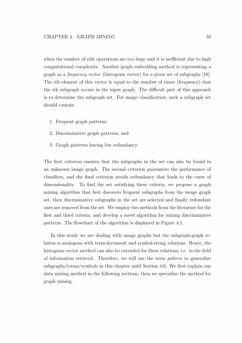
CHAPTER 4. GRAPH MINING 33
when the number of edit operations are too large and it is inefficient due to high
computational complexity. Another graph embedding method is representing a
graph as a frequency vector (histogram vector) for a given set of subgraphs [16].
The ith element of this vector is equal to the number of times (frequency) that
the ith subgraph occurs in the input graph. The difficult part of this approach
is to determine the subgraph set. For image classification, such a subgraph set
should contain
1. Frequent graph patterns,
2. Discriminative graph patterns, and
3. Graph patterns having low redundancy.
The first criterion ensures that the subgraphs in the set can also be found in
an unknown image graph. The second criterion guarantees the performance of
classifiers, and the final criterion avoids redundancy that leads to the curse of
dimensionality. To find the set satisfying these criteria, we propose a graph
mining algorithm that first discovers frequent subgraphs from the image graph
set, then discriminative subgraphs in the set are selected and finally redundant
ones are removed from the set. We employ two methods from the literature for the
first and third criteria, and develop a novel algorithm for mining discriminative
patterns. The flowchart of the algorithm is displayed in Figure 4.1.
In this study we are dealing with image graphs but the subgraph-graph re-
lation is analogous with term-document and symbol-string relations. Hence, the
histogram vector method can also be extended for these relations, i.e. in the field
of information retrieval. Therefore, we will use the term pattern to generalize
subgraphs/terms/symbols in this chapter until Section 4.6. We first explain our
data mining method in the following sections, then we specialize the method for
graph mining.

CHAPTER 4. GRAPH MINING 34
class 1
...class N
TRAINING TESTING
unknown image
Transforming images to graphs Transforming image to graph
node labels
Subgraph HistogramRepresentation
Image Set
Subgraph HistogramRepresentation
x1
. . .
xm
class 1
x1
. . .
xm
x1
. . .
xm
x1
. . .
xm
...class N
x1
. . .
xm
x1
. . .
xm
x1
. . .
xm
Vector Space Representation
Learning models for each class
Model 1 Model N...MathematicalModel
Decide onbest model
Transforming images to graphs
class 1
...class N
Subgraph Mining
...
Subgraph HistogramRepresentation
Graph Set
Subraph Set
for each class
Frequent subgraph mining
Image Graph Set
...Subgraph Set
Correlated subgraph mining
Subgraph Set
Redundancy-Awaresubgraph mining
Subgraph Set
...
...
Figure 4.1: Steps of graph mining algorithm

CHAPTER 4. GRAPH MINING 35
4.1 Foundations of Pattern Mining
Before the details of the algorithm, we would like to give some background in-
formation about pattern mining. In this chapter we use a similar notation to
Bringmann’s in [10] and the definitions in this section are mainly taken from that
study.
A definition of the task of finding all potentially interesting patterns is given
by Mannila and Toivonen [30]. The result of a data mining task is defined as a
theory depending on three parameters: a pattern language L, a dataset D, and a
selection predicate φ.
Definition 4.1 (Theory of φ with respect to L and D, [30]).
Assume a dataset D, a pattern language L for expressing properties or defining
subgroups of the data, and a selection predicate φ are given. The predicate φ
is used for evaluating whether a pattern π ∈ L defines a potentially interesting
subclass of D. The task of finding the theory of D with respect to L and φ is
defined as
Th(L,D, φ) = π ∈ L |φ(π,D) is true (4.1)
In our problem, the selection predicate φ is true if the pattern π is frequent,
discriminative and not redundant for the dataset D. We continue our definitions
with the matching function. Many graph mining researchers define matching
function as whether given subgraph occurs in example graph or not as in [10].
However, our study requires the number of times that a pattern occurs in an
example (Details will be given in the following sections). Therefore, we define the
matching function differently as follows.
Definition 4.2 (Matching Function).
Assume a pattern language L, a dataset D, and an evaluation predicate ϕ is
given. The number of valid occurrences of pattern π in x ∈ D is defined as
match : L ×D → Z0+ such that
match(π, x, ϕ) =∣∣h |h(π) ⊆ x ∧ ϕ(h, π, x) is true
∣∣ (4.2)
where h is called a mapping of pattern π into example x.

CHAPTER 4. GRAPH MINING 36
We use the terms valid occurrences and mapping in this definition instead
of simply saying the number of occurrences of π in x because the occurrence of
graph patterns in other graphs needs additional evaluations than term or symbol
patterns. We will describe some evaluation predicates for graph patterns in Sec-
tion 4.6; until there omitting the parameter ϕ from match(π, x, ϕ) for simplicity,
we have match(π, x) as an equivalent to the former.
The frequency vector described in the introductory paragraph of this chapter
is called propositionalization and defined below.
Definition 4.3 (Propositionalization, [10]).
Given a set of n patterns S = π1, . . . , πn, we define the feature vector of an
example x as−→fS(x) =
(match(π1, x), . . . ,match(πn, x)
)>. (4.3)
Total number of valid occurrences of a pattern in a dataset is called support of
that pattern. Again, we drop the evaluation predicate ϕ for the support definition.
Definition 4.4 (Support).
Given a pattern language L and a dataset D, support of a pattern π in D is
defined as
supp(π,D) =∑x∈D
match(π, x). (4.4)
And, our last definition in this section is frequency.
Definition 4.5 (Frequency).
Given a pattern language L, a dataset D, the frequency of a pattern π in D is
defined as
freq(π,D) =supp(π,D)
|D|. (4.5)
4.2 Frequent Pattern Mining
Our graph mining algorithm starts with discovering frequent patterns in the
dataset. Frequent patterns have broad application areas such as association

CHAPTER 4. GRAPH MINING 37
rule mining, indexing, clustering and classification [14]. We are interested in
the usefulness of frequent patterns in classification. Frequent pattern mining was
extensively studied in the data mining community and numerous algorithms has
been proposed in domains of different pattern types.
Assume dataset D is a set of examples where each example is labeled by one
class in a domain of classes C. The set of examples labeled by the class c is
denoted by Dc. In notation, we can say D =⋃i∈C Di. The problem of frequent
pattern discovery for class c can be formulated as finding all patterns generated
by the pattern language L, whose support in dataset Dc is grater than a threshold
θ suppc . The set of all frequent patterns for class c is
Fc =π ∈ L | supp(π,Dc) ≥ θ supp
c
. (4.6)
Assume we try to find frequent patterns in Dc. Let examples labeled by class
c be the set of positive examples, denoted by D+ and the set of all other examples
labeled by other classes be the set of negative examples, denoted by D−. Some
frequent pattern mining applications limit the support of frequent patterns in
negative set. In set definition, it is given by
Fc =π ∈ L | supp(π,D+) ≥ θ supp
+ ∧ supp(π,D−) ≤ θ supp−. (4.7)
Since the size and property of a dataset varies among classes we can set
different thresholds for each class. In our study, we mine the set of frequent
patterns for each class, then they will be used as input to the next step which is
correlated pattern mining.
4.3 Class Correlated Pattern Mining
Our second objective for the selected patterns is being discriminating for classi-
fication. Assume a dataset D labeled with three classes such as D1, D2 and D3.
A discriminative pattern is expected to be found in examples of one class and
not in the other classes. Such a relation between a pattern and a class is called

CHAPTER 4. GRAPH MINING 38
correlation. Two types of correlation have been defined: Positive and negative
correlation. Assume we focus on finding correlated patterns of the first class. A
pattern observed in only the first class, D1, is called positively correlated pattern
with the first class or shortly class-correlated pattern. In contrast, a negatively
correlated pattern is found in all classes except the first class (in this case D2 and
D3). Both positive and negative correlation can be useful for classification. For
example, an unseen example can be assigned to the first class if it includes posi-
tively correlated patterns with the first class. On the other hand, observation of
negatively correlated patterns with the first class in an unseen example indicates
that the example does not belong to the first class. Previous works on class-
correlated patterns in [10, 33] only involve two-class datasets and the study in
[34] handles multi-class correlation. However, all previous methods on correlated
pattern mining base on binary matching function. Hence, more than one occur-
rences of a pattern in an example have the same effect with a single occurrence on
correlation measure. We propose a novel technique to mine multi-class correlated
patterns, in which the number of occurrences are taken into consideration. Unlike
previous works, we are only dealing with positively correlated patterns and do
not consider negatively correlated patterns. The following subsection explains
the mathematical modeling of patterns in examples and the second subsection
gives details of mining correlated patterns according to the model.
4.3.1 Mathematical Modeling of Pattern Support
We start our algorithm by deriving the probability that a pattern π occurs k times
in an example. Let x be a document containing Nt terms and the probability that
a randomly selected term t from x is an instance of the pattern π be a Bernoulli
distribution with PrT = π = p and PrT 6= π = 1 − PrT = π = 1 − p.
Then, the probability that x contains π for k times is a Binomial distribution
with
PrK = k =
(Nt
k
)pk(1− p)Nt−k for k = 0, 1, 2, . . . , Nt. (4.8)
We now define the expected number of occurrences as λ = pNt. We generalize

CHAPTER 4. GRAPH MINING 39
0 5 10 15 20 25 300
0.05
0.10
0.15
0.20
0.25
0.30
0.35
0.40
k
λ = 1λ = 4λ = 8λ = 16
Pois(k|λ)
Figure 4.2: Poisson distributions with four different expected values.
this probability by assuming that the size of document is unbounded, then
PrK = k = limNt→∞
(Nt
k
)pk(1− p)Nt−k =
λke−λ
k!for k ∈ Z0
+. (4.9)
The limiting case of Binomial distribution is known as Poisson distribution
and is denoted by Pois(k |λ). Poisson distributions with different expected values
are shown in Figure 4.2.
We model the term frequency in a document as a Poisson distribution. How-
ever, Church and Gale claim in [15] that term rates vary from author-to-author,
topic-to-topic, document-to-document, section-to-section, and paragraph-to-
paragraph (and theme-to-theme if we consider images). They propose Poisson
mixture to capture much of this heterogeneous structure by allowing the Poisson
parameter λ to vary over documents. It is subject to a density function ϑ aimed
to capture dependencies on hidden variables such author, topic, etc.
Definition 4.6 (Poisson Mixtures, [15]).
Given the density function ϑ to capture dependencies on hidden variables, the
general form of a Poisson mixture is
p(k) =
∫ ∞0
ϑ(λ)Pois(k |λ) dλ (4.10)
where ϑ density function should integrate to 1. That is,∫∞
0ϑ(λ) dλ = 1.

CHAPTER 4. GRAPH MINING 40
In this study we will use a mixture of finite number of Poisson distributions.
Therefore, we use coefficients αj instead of ϑ function:
p(k) =m∑j=1
αjPois(k |λj) (4.11)
where∑m
j=1 αj = 1 such that αj ≥ 0 for j = 1, . . . ,m.
The next step of modeling is parameter estimation for Poisson mixtures from
a dataset. The Expectation-Maximization(EM) Algorithm can be used for the
solution to the maximum-likelihood parameter estimation problem. The EM
algorithm is exhaustively described in [6] for Gaussian mixture model and we
will extend this study for Poisson mixture model.
We have a density function p(k |Θ) governed by the set of parameters Θ =
(α1, . . . , αm, λ1, . . . , λm) and a dataset of size n, supposedly drawn independently
from this distribution, i.e. K = k1, . . . , kn. The resulting density for samples is
p(K |Θ) =n∏i=1
p(ki |Θ) = L(Θ | K) (4.12)
where L(Θ | K) is called the likelihood function. The goal of EM algorithm is to
find Θ∗ iteratively where
Θ∗ = arg maxΘ
L(Θ | K). (4.13)
We assume that a complete data set exists as a combination of the observed
but incomplete data K and the missing data Z. The EM algorithm seeks to find
the maximum likelihood estimate (MLE) of the marginal likelihood by iteratively
applying the following two steps:
Expectation step: The expected value of the log likelihood function is calcu-
lated with respect to the unknown data Z given the observed data K and the
current parameter estimates Θ(i−1).
Q(Θ,Θ(i−1)
)= E
[log p(K,Z |Θ)
∣∣K,Θ(i−1)]. (4.14)
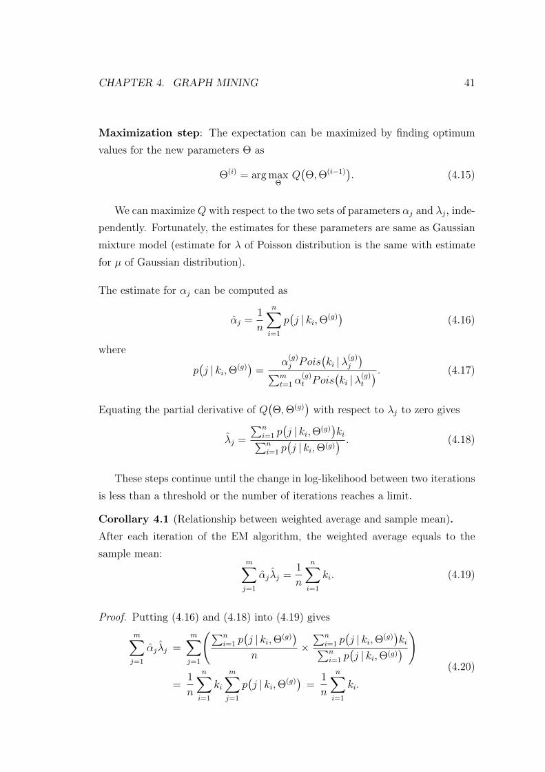
CHAPTER 4. GRAPH MINING 41
Maximization step: The expectation can be maximized by finding optimum
values for the new parameters Θ as
Θ(i) = arg maxΘ
Q(Θ,Θ(i−1)
). (4.15)
We can maximize Q with respect to the two sets of parameters αj and λj, inde-
pendently. Fortunately, the estimates for these parameters are same as Gaussian
mixture model (estimate for λ of Poisson distribution is the same with estimate
for µ of Gaussian distribution).
The estimate for αj can be computed as
αj =1
n
n∑i=1
p(j | ki,Θ(g)
)(4.16)
where
p(j | ki,Θ(g)
)=
α(g)j Pois
(ki |λ(g)
j
)∑mt=1 α
(g)t Pois
(ki |λ(g)
t
) . (4.17)
Equating the partial derivative of Q(Θ,Θ(g)
)with respect to λj to zero gives
λj =
∑ni=1 p
(j | ki,Θ(g)
)ki∑n
i=1 p(j | ki,Θ(g)
) . (4.18)
These steps continue until the change in log-likelihood between two iterations
is less than a threshold or the number of iterations reaches a limit.
Corollary 4.1 (Relationship between weighted average and sample mean).
After each iteration of the EM algorithm, the weighted average equals to the
sample mean:m∑j=1
αjλj =1
n
n∑i=1
ki. (4.19)
Proof. Putting (4.16) and (4.18) into (4.19) gives
m∑j=1
αjλj =m∑j=1
(∑ni=1 p
(j | ki,Θ(g)
)n
×∑n
i=1 p(j | ki,Θ(g)
)ki∑n
i=1 p(j | ki,Θ(g)
) )
=1
n
n∑i=1
ki
m∑j=1
p(j | ki,Θ(g)
)=
1
n
n∑i=1
ki.
(4.20)

CHAPTER 4. GRAPH MINING 42
0 5 10 15 200
5
10
15
20
k
0
0.05
0.1
0.15
0.2
p (k
)
hist
(k)
Figure 4.3: A sample histogram of a dataset with 100 elements and fitting mix-tures of 3 Poisson distributions to this histogram are shown in blue and red,respectively.
This shows the equality between weighted average and sample mean.
A sample histogram and the Poisson mixture trained on this data can be seen
in Figure 4.3.
Returning to our problem, we employ Poisson mixture to model the proba-
bility of the term frequency of pattern π in a document randomly selected from
the corpus D. Thus, the dataset used in the EM algorithm is K = k1, . . . , kn =match(π, x1), . . . ,match(π, xn)
for D = x1, . . . , xn.
4.3.2 Correlated Patterns
In this section we give details of correlated-pattern mining according the proba-
bility calculations drawn in the previous section. A pattern π is called correlated
with a class c ∈ C if that pattern is frequently observed in Dc while it is sel-
dom seen in Dc′ for all c′ ∈ C such that c′ 6= c. Using the support of a pattern
in correlation measure may result in wrong classification of unknown documents
because the support in a dataset does not give any frequency information of the
pattern in individual documents. For example, a pattern may occur frequently

CHAPTER 4. GRAPH MINING 43
in some documents of a dataset while not occurring in other documents. There-
fore, frequency analysis of a pattern should be done using the frequency in each
document as in the previous section.
Assume a pattern π which does not occur in a dataset D, in notational form
supp(π,D) = 0, then training the EM algorithm on such a case produces the
following density function pref, which we call the reference distribution,
pref(k) =
1 if k = 0
0 otherwise.(4.21)
As understood from its name we employ this density function for comparison
with other distributions in correlation measurement. Let pc(k |π,Dc) denote the
Poisson mixture distribution trained for pattern π on dataset Dc. We compute the
distance (dissimilarity) between density functions pc(k | π,Dc) and pref(k) using
the Earth mover’s distance technique.
In terms of positive correlation between pattern π and class c, the distance
between pc(k |π,Dc) and pref(k) should be as large as possible while the distance
between pc′(k | π,Dc′) and pref(k) should be as small as possible for all c′ ∈ C such
that c′ 6= c.
Earth mover’s distance is proposed by [38] to measure the dissimilarity be-
tween not only probability distributions but also histograms and clusters. Levina
and Bickel [27] showed that Earth mover’s distance is conceptually equivalent to
Mallow distance on probability distributions but we continue calling it the Earth
mover’s distance in this study.
Definition 4.7 (Earth mover’s distance, [38]).
Let Q =
(q1, wq1), . . . , (qr, wqr)
be the signature with r clusters, where qi is
the representative of the ith data cluster and wqi is the number of points in the
cluster. Let Q′ =
(q′1, wq′1), . . . , (q′s, wq′s)
be the second signature with s clusters;
and D =[dij]
is the ground distance matrix where dij is some measure of distance
between clusters of qi and q′j. Earth mover’s distance is computed by solving the
optimization problem of finding a flow F =[fij], with fij the flow from qi to q′j,

CHAPTER 4. GRAPH MINING 44
that minimizes the overall work
Minimize WORK(Q,Q′,F) =r∑i=1
s∑j=1
dijfij (4.22)
Subject to fij ≥ 0, 1 ≤ i ≤ r, 1 ≤ j ≤ s, (4.23)s∑j=1
fij ≤ wqi , 1 ≤ i ≤ r, (4.24)
r∑i=1
fij ≤ wq′j , 1 ≤ j ≤ s, (4.25)
r∑i=1
s∑j=1
fij = min
(r∑i=1
wqi ,s∑j=1
wq′j
). (4.26)
Once the optimal flow f ∗ij is found, the Earth Mover’s distance between Q and
Q′ is defined as
EMD(Q,Q′) =
∑ri=1
∑sj=1 f
∗ijdij∑r
i=1
∑sj=1 f
∗ij
. (4.27)
According to (4.24) and (4.25), we can transform a discrete distribution p(k)
defined in Z0+ to the signature form by
P =(k, p(k)
) ∣∣ k ∈ Z0+ ∧ p(k) > 0
. (4.28)
The signature size of a Poisson mixture may be infinite, or the signature may
be reduced to finite elements if the condition in (4.28) is changed to p(k) > ε for
a small number ε.
From (4.28), the signature form of the distribution pref(k) becomes
Pref =
(q′1, wq′1)
=
(0, 1)
. Let Pc denote the signature form of probability
distribution pc(k | π,Dc), then the optimal flow from Pc to Pref is
f ∗ij =
pc(ki | π,Dc) if j = 1
0 otherwise.(4.29)

CHAPTER 4. GRAPH MINING 45
Constraint (4.26) is actually equal to∑r
i=1
∑sj=1 fij = 1 for probability dis-
tributions and this constraint forces all earth to flow from every qi to the only
element of Pref, which is q′1. Finally, we need to define a ground distance function,
d : Z2 → R0+, for the ground distance matrix D =
[dij]
=[d(qi, q
′j)]. Then, the
Earth mover’s distance is computed as
EMD(Pc, Pref) =
∑ri=1
∑sj=1 f
∗ijdij∑r
i=1
∑sj=1 f
∗ij
=r∑i=1
pc(ki | π,Dc) d(ki, 0)
=r∑i=1
pc(ki | π,Dc) d′(ki)
= E[d′(K)
∣∣ π,Dc](4.30)
where d′(k) = d(k, 0) and K is a random variable K ∈ k1, . . . , kr or more
generally K ∼ Z0+. One possible definition of the distance function for two
distributions is d(i, j) = 1 − e−ξ|i−j| where ξ is a regulation constant. Note that
d(i, j) ∈ [0, 1], and
d′(i) = 1− e−ξi for i ≥ 0. (4.31)
Accordingly, the Earth mover’s distance is in the same range [0, 1] due to
definition of distance function. One reason why we choose this nonlinear function
is to prevent outliers in the dataset from dominating the Earth mover’s distance.
The regulation constant ξ is used for this purpose.
Assume we try to find correlated patterns of class c. Each frequent pattern
π ∈ Fc mined in the previous section should be tested by a correlation measure
γ based on the Earth mover’s distance. The correlation measure that we define
has two parameters: positive distance pcπ and negative distance ncπ. The positive
distance is the Earth mover’s distance between Pc and Pref for dataset Dc. On
the other hand, the negative distance is computed from datasets Dc′ for all c′ ∈ Csuch that c′ 6= c. In terms of classification, the class which will cause confusion
with class c is the one with the maximum Earth mover’s distance between Pc′
and Pref from all c′ ∈ C such that c′ 6= c. Thus, the positive and negative distance
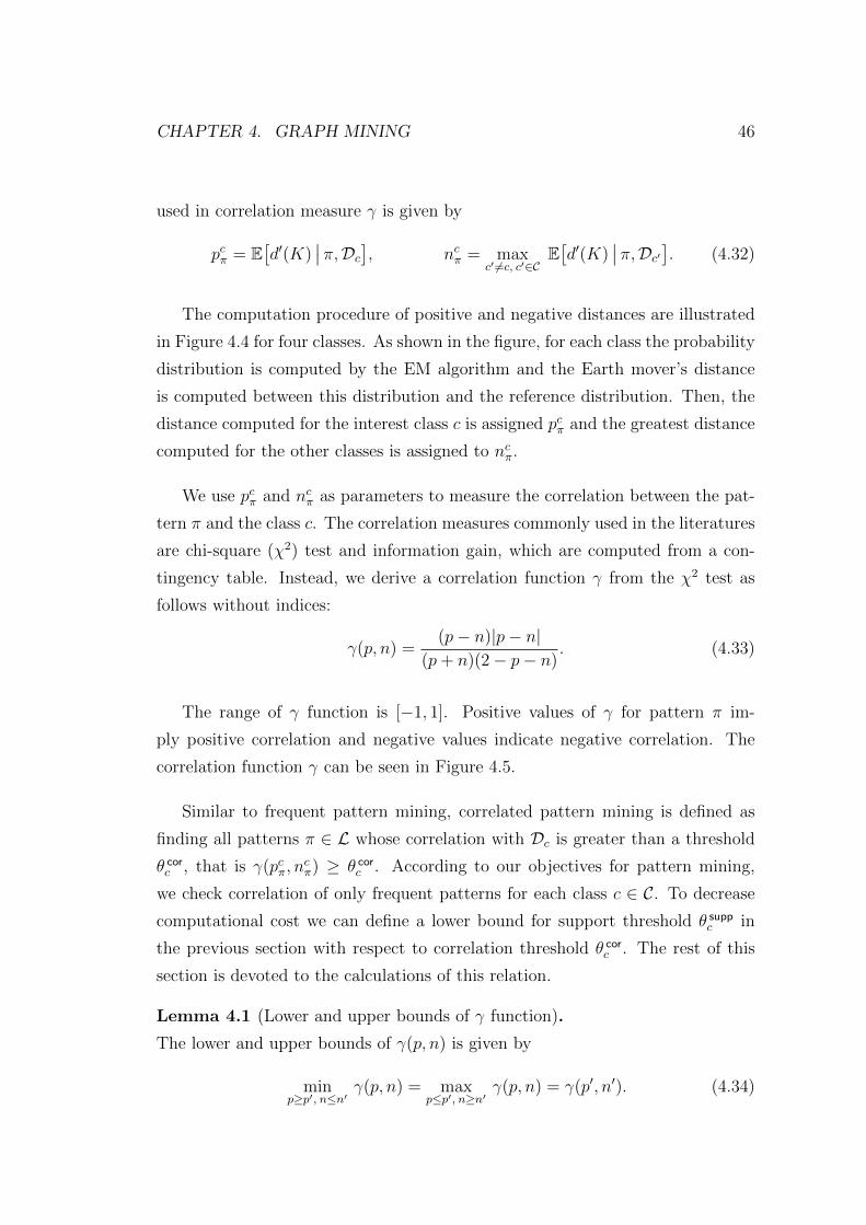
CHAPTER 4. GRAPH MINING 46
used in correlation measure γ is given by
pcπ = E[d′(K)
∣∣ π,Dc], ncπ = maxc′ 6=c, c′∈C
E[d′(K)
∣∣ π,Dc′]. (4.32)
The computation procedure of positive and negative distances are illustrated
in Figure 4.4 for four classes. As shown in the figure, for each class the probability
distribution is computed by the EM algorithm and the Earth mover’s distance
is computed between this distribution and the reference distribution. Then, the
distance computed for the interest class c is assigned pcπ and the greatest distance
computed for the other classes is assigned to ncπ.
We use pcπ and ncπ as parameters to measure the correlation between the pat-
tern π and the class c. The correlation measures commonly used in the literatures
are chi-square (χ2) test and information gain, which are computed from a con-
tingency table. Instead, we derive a correlation function γ from the χ2 test as
follows without indices:
γ(p, n) =(p− n)|p− n|
(p+ n)(2− p− n). (4.33)
The range of γ function is [−1, 1]. Positive values of γ for pattern π im-
ply positive correlation and negative values indicate negative correlation. The
correlation function γ can be seen in Figure 4.5.
Similar to frequent pattern mining, correlated pattern mining is defined as
finding all patterns π ∈ L whose correlation with Dc is greater than a threshold
θ corc , that is γ(pcπ, n
cπ) ≥ θ cor
c . According to our objectives for pattern mining,
we check correlation of only frequent patterns for each class c ∈ C. To decrease
computational cost we can define a lower bound for support threshold θ suppc in
the previous section with respect to correlation threshold θ corc . The rest of this
section is devoted to the calculations of this relation.
Lemma 4.1 (Lower and upper bounds of γ function).
The lower and upper bounds of γ(p, n) is given by
minp≥p′, n≤n′
γ(p, n) = maxp≤p′, n≥n′
γ(p, n) = γ(p′, n′). (4.34)

CHAPTER 4. GRAPH MINING 47
0,0
0,5
1,0
p (k)4
k
P4
0,0
0,5
1,0
p (k)1
k
P1
0,0
0,5
1,0
p (k)3
k
P30,0
0,5
1,0
0
p (k)ref
k
Pref0,0
0,5
1,0
p (k)2
k
P2
P4
EMD
( , )P
ref
P2EMD ( ,
)Pref
P3
EMD ( , )P
ref
P 1
EMD
( ,
)
P ref
Figure 4.4: The procedure for positive and negative distance computation isillustrated for four classes. The interest class is the second one and the distancesare computed as p = EMD(P2, Pref) and n = EMD(P3, Pref).

CHAPTER 4. GRAPH MINING 48
00.25
0.50.75
1
00.25
0.50.75
1−1
−0.75
−0.5
−0.25
0
0.25
0.5
0.75
1
np
−0.8
−0.7
−0.6−0.5−0.4
−0.3
−0.3
−0.2
−0.2
−0.1
−0.1
−0.1
0
0
0
0.1
0.1
0.1
0.2
0.2
0.3
0.3
0.4
0.4
0.50.6
0.70.8
np
γ ( p, n )
0 0.2 0.4 0.6 0.8 10
0.2
0.4
0.6
0.8
1
γ ( p, n )
Figure 4.5: The correlation function γ(p, n)
Proof. Partial derivatives give the limits of γ(p, n).
∂γ(p, n)
∂p=
2(p− 2pn+ 3n− 2n2)|p− n|(p+ n)2(2− p− n)2
=2(p(1− n) + n(3− p− 2n)
)|p− n|
(p+ n)2(2− p− n)2.
(4.35)
Due to definition of d(i, j), the pn space is defined for 0 ≤ p, n ≤ 1. Hence, all
terms in (4.35) are nonnegative. As a result, ∂γ(p,n)∂p≥ 0 and we can say
γ(p, n) ≥ γ(p′, n) for 0 ≤ p′ ≤ p ≤ 1. (4.36)
Similarly,
∂γ(p, n)
∂n= −2(3p− 2p2 − 2pn+ n)|p− n|
(p+ n)2(2− p− n)2
= −2(p(3− 2p− n) + n(1− p)
)|p− n|
(p+ n)2(2− p− n)2.
(4.37)
All terms in (4.37) are nonnegative. Consequently, ∂γ(p,n)∂n
≤ 0 and we can also
say
γ(p, n) ≥ γ(p, n′) for 0 ≤ n ≤ n′ ≤ 1. (4.38)
Combining (4.36) and (4.38) gives (4.34).

CHAPTER 4. GRAPH MINING 49
Theorem 4.1 (Correlation–Positive support relation).
For a given pattern π ∈ L, if γ(pcπ, ncπ) ≥ θ cor
c for some thresholds θ corc ≥ 0
where pcπ and ncπ are computed from Dc and Dc′ for all c′ ∈ C such that c′ 6= c,
respectively, then
supp(π,Dc) ≥ −|Dc|
1− e−ξln
(1− θ cor
c
1 + θ corc
). (4.39)
Proof. According to Lemma 4.1, we can say
γ(pcπ, 0) ≥ γ(pcπ, ncπ) ≥ θ cor
c . (4.40)
Putting (4.33) into (4.40),
pcπ2− pcπ
≥ θ corc ⇒ pcπ ≥
2θ corc
1 + θ corc
. (4.41)
Now, we compute pcπ from (4.32). Let the parameters of Poisson mixture
be Θ = (α1, . . . , αm, λ1, . . . , λm) found by the EM algorithm for pc(k | π,Dc) on
observed data K =match(π, x1), . . . ,match(π, xn)
where Dc = x1, . . . , xn.
The positive distance is computed as
pcπ = E[d′(K)
∣∣ π,Dc] =∞∑i=0
pc(i |π,Dc) d′(i)
=∞∑i=0
m∑j=1
αjPois(i |λj) d′(i)
=∞∑i=0
m∑j=1
αjλij e
−λj
i!(1− e−ξi)
=m∑j=1
αje−λj
∞∑i=0
(λiji!− (λje
−ξ)i
i!
)
=m∑j=1
αje−λj(eλj − e(λje
−ξ))
=m∑j=1
(αj − αje−λj(1−e
−ξ))
= 1−m∑j=1
αje−λjd′(1).
(4.42)

CHAPTER 4. GRAPH MINING 50
Introducing ε = d′(1) results in pcπ = 1 −∑m
j=1 αje−ελj . Combining (4.41) and
(4.42) gives
1−m∑j=1
αje−ελj ≥ 2θ cor
c
1 + θ corc
⇒m∑j=1
αje−ελj ≤ 1− θ cor
c
1 + θ corc
. (4.43)
Before continuing the proof, we need to define convex function and Jensen’s
inequality.
Definition 4.8 (Convex function).
Let C be a convex subset of Rn. A function f : C → R is called convex if
f(ax1 + (1− a)x2
)≤ af(x1) + (1− a)f(x2) for a ∈ [0, 1] and x1 6= x2. (4.44)
See Figure 4.6 for a sample convex function.
Theorem 4.2 (Jensen’s inequality).
If f is a convex function and X is a random variable, then
f(E[X]
)≤ E
[f(X)
]. (4.45)
In finite form, numbers x1, x2, . . . , xn are in domain of f , and positive weights ai
such that∑n
i=1 ai = 1, Jensen’s inequality can be stated as
f
(n∑i=1
aixi
)≤
n∑i=1
aif(xi). (4.46)
We define function f : R → R such as f(x) = e−εx. This function is strictly
convex because d2f(x)dx2
= ε2e−εx > 0. Now, we can extend (4.43) using (4.46) and
f function as follows
m∑j=1
αjf(λj) ≤1− θ cor
c
1 + θ corc
⇒ f
(m∑j=1
αjλj
)≤ 1− θ cor
c
1 + θ corc
. (4.47)
Substituting f(x) with e−εx,
⇒ exp
(−ε
m∑j=1
αjλj
)≤ 1− θ cor
c
1 + θ corc
⇒ −εm∑j=1
αjλj ≤ ln
(1− θ cor
c
1 + θ corc
).
(4.48)

CHAPTER 4. GRAPH MINING 51
x1 x2a x1 + (1 − a) x2
f (a x1 + (1 − a) x )2
a f (x )1 + (1 − a) f (x )2
Figure 4.6: Plot of a convex function f
Using (4.19) and the definition of K, we can say
m∑j=1
αjλj =1
n
n∑i=1
ki =1
n
n∑i=1
match(π, xi) =1
nsupp(π,Dc). (4.49)
Finally, using (4.48) and (4.49), and substituting ε with 1− e−ξ, and n with |Dc|makes
supp(π,Dc) ≥ −|Dc|
1− e−ξln
(1− θ cor
c
1 + θ corc
). (4.50)
This completes our proof.
The support threshold should be defined considering this relation. Likewise,
the positive distance of a frequent pattern depends on the support threshold as
follows.
Corollary 4.2 (Support threshold–positive distance relation).
Let π ∈ L be a frequent pattern whose support is greater than the threshold θ suppc
for dataset Dc, then
pcπ ≥ 1− exp
(−θ
suppc
|Dc|(1− e−ξ
)). (4.51)

CHAPTER 4. GRAPH MINING 52
Proof. Using same convex f function of the previous proof in (4.42), we get
pcπ = 1−m∑j=1
αje−λjd′(1) = 1−
m∑j=1
αjf(λj)
≥ 1− f( m∑
j=1
αjλj
)
≥ 1− exp
(−d′(1)
m∑j=1
αjλj
)
≥ 1− exp
(−d′(1)
nsupp(π,Dc)
)≥ 1− exp
(−(1− e−ξ
)θ suppc
|Dc|
).
(4.52)
4.4 Redundancy-Aware Top-k Patterns
After two steps of pattern mining, we have a set of frequent and class-correlated
patterns. Usage of this set for classification suffers from curse of dimensionality
because the set contains many redundant patterns and its size is not limited. Let
the graph patterns in Figure 4.7 be frequent and correlated patterns. As seen in
the figure, the only difference between patterns is an edge. The pattern in 4.7(b)
is found everywhere the pattern in 4.7(a) is found. The number of occurrences
of these two patterns is very close or same in every example of a dataset. As a
result, the significance of these patterns together in a set is equal to significance
of only one of them. In this section we seek a set of most significant k patterns,
which has low redundancy. The method described in this section is suggested by
Xin et al. in [45]. This study gives the definitions for pattern significance and
pattern redundancy as a part of formal problem formulation.
Definition 4.9 (Pattern Significance, [45]).
Given pattern language L, a significance measure is a function S : L → R, S(π)
is the degree of interestingness (or usefulness) of pattern π.

CHAPTER 4. GRAPH MINING 53
(a) (b)
Figure 4.7: Two sample redundant graph patterns
Since we focus on classification problem in this study, we choose γ function
as a measure of pattern significance, so S(π) = γ(pcπ, ncπ). Xin et al. extend the
pattern significance to combined significance and relative significance. Let the
combined significance S(π, π′) denote the collective significance of two individual
patterns π and π′. Before defining relative significance, we need to define pat-
tern redundancy. Given significance measures, pattern redundancy is defined as
follows.
Definition 4.10 (Pattern Redundancy, [45]).
Given the significance measure S, the redundancy R between two patterns π and
π′ is defined as R(π, π′) = S(π) + S(π′)− S(π, π′).
Subsequently, the relative significance of π given π′ is S(π |π′) = S(π)−R(π, π′).
Assuming that combined significance is not less than the significance of any in-
dividual pattern and not grater than the sum of two individual significance; then
the redundancy between patterns π and π′ should satisfy
0 ≤ R(π, π′) ≤ min(S(π), S(π′)
). (4.53)
According to [45], the ideal redundancy measure R(π, π′) is usually hard to
obtain. Therefore, they suggest using distance between patterns in order to mea-
sure patterns redundancy.
Definition 4.11 (Pattern Distance, [45]).
A distance measure D : L× L → [0, 1] is a mapping from two patterns π, π′ ∈ Lto a value in [0, 1], where 0 means π and π′ are completely relevant and 1 means
π and π′ are totally independent.

CHAPTER 4. GRAPH MINING 54
The pattern distance is used for approximating the pattern redundancy. The
following equation which satisfies (4.53) is given in [45].
R(π, π′) =(1−D(π, π′)
)×min
(S(π), S(π′)
). (4.54)
The distance between two patterns depends on the pattern structure. It can
be the edit distance for sequences or the graph edit distance [37] for graph pat-
terns. Alternatively, in the distance function we use the number of occurrences
of patterns in a dataset because it provides the correlation between two patterns
in document level. We define the distance function using cosine similarity in the
field of information retrieval as follows.
D(π, π′) = 1− cosD(π, π′) = 1− u · v‖u‖ ‖v‖
(4.55)
where u =−→fD(π) and v =
−→fD(π′). We use the whole dataset D =
⋃i∈C Di, in
distance computation where−→fD is defined as
−→fD(π) =
(match(π, x1), . . . ,match(π, xn)
)>(4.56)
where D = x1, . . . , xn. By the help of this distance function, we try to find a
set of patterns which occur in not only some examples of the dataset Dc in which
we are interested, but in all examples of Dc if possible.
Finally, the formulation is extended to a set of k patterns Pk ⊂ L. Let G be
a significance measure for a set of patterns, and the redundancy measure for a
set of patterns be L which is hard to obtain [45]. In general,
Ggen(Pk) =k∑i=1
S(πi)− L(Pk). (4.57)
The authors of [45] suggest two heuristic evaluation functions Gas (average
significance) and Gms (marginal significance). We prefer using marginal signif-
icance so we only explain this function. The computational model for the new
concept is a graph called redundancy graph:
Definition 4.12 (Redundancy Graph, [45]).
Given a significance measure S and a redundancy measure R for individual pat-
terns, a redundancy graph of a set of k patterns Pk is a weighted graph where

CHAPTER 4. GRAPH MINING 55
each pattern, πi, corresponds to node i whose weight is pattern significance S(πi)
and the weight on an edge (i, j) is the redundancy R(πi, πj).
Marginal significance of a set of patterns is computed as
Gms(Pk) =k∑i=1
S(πi)− w(MST (Pk)
)(4.58)
where w(MST (Pk)
)denotes the sum of edge weights on the maximum span-
ning tree of the redundancy graph. Given a pattern language L, the problem of
maximal marginal significance (MMS) is to find a set of k patterns Pk such that
Gms(Pk) is maximized. Finally, the study [45] gives Algorithm 2 for the problem
of MMS.
According to our definitions of pattern significance and distance, we obtain
a redundancy-aware set of frequent top-k patterns in terms of correlation. We
denote this set by Sc for class c ∈ C and we apply these mining steps for each
class. Then, all selected patterns are collected in one set S which will be used for
classification. This completes the process of finding a set of patterns satisfying
our objectives given in the beginning of this chapter.
4.5 Summary of the Mining Algorithm
The procedure so far is aiming to find a set of patterns satisfying our objectives
given at the beginning of this chapter. Each step can be considered as a pattern
filter which is responsible for one criterion. To reduce the computational cost,
the filters are connected in series, in other words the input patterns of a filter is
the output of another. The order of filters are same with the section order. First,
the patterns generated by the language L are tested for support with respect to
the threshold θ suppc and the frequent ones are collected in the set Fc. Next, the
members of this set are tested for the correlation with respect to the threshold
θ corc and the set Rc contains patterns which are both frequent and correlated.
The last filter seeks a small subset Pc which has significant and not redundant

CHAPTER 4. GRAPH MINING 56
Algorithm 2 Greedy Algorithm for MMS, [45]
Input: A set of n patterns, L = π1, . . . , πnNumber of output patterns, kSignificance measure, SDivergence measure, D
Output: Top-k pattern set, Pk1: t← 0, T ← maxπ∈L S(π)2: selected[i]← false for i = 1, . . . , n3: removed[i]← false for i = 1, . . . , n4: for i← 1 to k do5: if there is no pattern left then6: T ← T+t
2
7: goto line 28: end if9: πs ← the most significant pattern s.t.
selected[s] = false and removed[s] = false10: selected[s]← true11: removed[s]← true12: for j ← 1 to n do13: if removed[j] = false and selected[j] = false then14: if S(πj |πs) ≤ T+t
2then
15: removed[j]← true16: end if17: end if18: end for19: end for20: if there are patterns left (πi s.t. removed[i] = false) then21: t = t+T
2
22: goto line 223: end if24: return selected k-patterns (πi s.t. selected[i] = true)

CHAPTER 4. GRAPH MINING 57
patterns. These steps are repeated for each class c ∈ C and then the patterns
satisfying these criteria for some classes are grouped into the final set S which is
used for classification. Algorithm 3 shows the steps of the mining algorithm.
Algorithm 3 Pattern Mining Algorithm
Input: A pattern language, LA dataset D labeled with classes CSupport thresholds, θ supp
c for each c ∈ CCorrelation thresholds, θ cor
c for each c ∈ CNumber of top patterns for each class, kAn evaluation predicate, ϕ
Output: A pattern set, S1: S ← ∅2: for each class c ∈ C do3: Fc ← ∅4: for each pattern π generated by L do5: if supp(π,Dc, ϕ) ≥ θ supp
c then supp defined in Definition 4.46: Fc ← Fc ∪ π7: end if8: end for9: Rc ← ∅
10: for each pattern π ∈ Fc do11: compute pcπ and ncπ on D defined in (4.32)12: if γ(pcπ, n
cπ) ≥ θ cor
c then γ defined in (4.33)13: Rc ← Rc ∪ π14: end if15: end for16: for each pattern π ∈ Rc do17: compute pattern significance as S[π] = γ(pcπ, n
cπ)
18: for each pattern π′ ∈ Rc do19: compute pattern distances D[π, π′] = 1−cosD(π, π′) defined in (4.55)20: end for21: end for22: Pc ← output of Greedy Algorithm for MMS with Rc, k, S and D23: S ← S ∪ Pc24: end for25: return S
We can analyze search regions of patterns in the pn space. Assume that the
support threshold θ suppc is chosen greater than the lower bound given in Theo-
rem 4.1. The members of Fc are found in the shaded area (union of dark and

CHAPTER 4. GRAPH MINING 58
n
p
0 10
1
supp(π,Dc) −|Dc|1− e−ξ ln
1− θ corc1 + θ corc( )
1− exp −θsuppc
|Dc|1− e−ξ )(( )
θ suppc
2θ corc1 + θ corc
=
θ corc
supp(π,Dc) =
Plot of γ
Figure 4.8: The pn space showing the search regions for the first two steps of thealgorithm. The shaded area (union of dark and light gray) represent the domainregion of Fc and dark gray area represents the domain region of Rc.
light gray) in Figure 4.5 according to Corollary 4.2. After the correlation check,
the region of Rc is reduced to the dark gray area in the figure. The final step
does not reduce the search region in the pn space because set Pc may contain a
pattern π on the correlation boundary S(π) = θ corc because of the redundancy
definition.
Someone may claim that changing the order of the first two steps causes
the computational cost to reduce. However, it is not sensible most of the time
because the support test has negligible computation cost compared to the cor-
relation test which includes the execution of the EM algorithm. Furthermore, a
structural language which has a generalization relation among its patterns enables
us to define an anti-monotonic matching function. Such a function provides the
pruning ability in generating frequent patterns of the language using the pattern
growth approach. For example, many frequent graph mining algorithms generate
subgraphs from the dataset. They start generating subgraphs from one node
subgraphs and continue generating new subgraphs by adding nodes and edges to

CHAPTER 4. GRAPH MINING 59
the previous ones. In generating process, the subgraphs whose support in the
dataset is less than the threshold are eliminated and only the frequent ones are
preserved. The algorithm stops when no new subgraph can be generated from
the frequent subgraphs.
To recall the theory of φ in Section 4.1, the mining algorithm also tries to find
the theory of a selection predicate. Now, we can define the selection predicate φ
to find the theory with respect to the language L and the dataset D as follows.
φ(π,D) =
true if ∃c ∈ C : supp(π,Dc) ≥ θ suppc ∧ γ(pcπ, n
cπ) ≥ θ cor
c ∧ π ∈ Pc
false otherwise.
(4.59)
4.6 Graph Patterns
In this section, we narrow down the theoretical concepts in the previous sections
to graph patterns. All computations in Sections 4.2 to 4.4 are based on definitions
in Section 4.1 and the abstraction of these definitions for all pattern types is based
on the evaluation predicate ϕ. We will define alternative ϕ predicates for graph
patterns. Therefore, we start to use the following graph terminology:
pattern π −→ subgraph g
example x −→ image (input) graph G
dataset D −→ graph set G
Accordingly, a mapping h of pattern π into example x, given in the matching
function definition is called subgraph isomorphism in the graph terminology. The
definition is given by Fiedler and Borgelt as follows.
Definition 4.13 (Subgraph isomorphism, [18]).
Let g = (Vg, Eg, `g) and G = (VG, EG, `G) be two labeled graphs. A sub-
graph isomorphism of g to G is an injective function h : Vg → VG satisfy-
ing ∀v ∈ Vg : `g(v) = `G(h(v)
)and ∀(u, v) ∈ Eg :
(h(u), h(v)
)∈ EG ∧

CHAPTER 4. GRAPH MINING 60
(a) subgraph (b) input graph
Figure 4.9: An example for overlapping embeddings
`g((u, v)
)= `G
((f(u), f(v)
)).
Every subgraph isomorphism of subgraph g to image graph G defines an
embedding of subgraph g. Different embeddings of g may refer to same nodes in
G as in Figure 4.9. They are called overlapping subgraph isomorphism.
Definition 4.14 (Overlapping subgraph isomorphism, [18]).
Let g = (Vg, Eg, `g) and G = (VG, EG, `G) be two labeled graphs, h1 and h2 two
subgraph isomorphisms of g to G, and Vi =v ∈ VG
∣∣ ∃u ∈ Vg : v = hi(u)
,
Ei =e ∈ EG
∣∣∃(u, v) ∈ Eg : e =(hi(u), hi(v)
)for i = 1 or 2. Two subgraph
isomorphisms h1 and h2 are called overlapping iff V1 ∩V2 6= ∅ and written h1h2.
Also, h1 and h2 are called equivalent, written h1 h2, iff V1 = V2 and E1 = E2.
Finally, h1 and h2 are called identical, written h1 ≡ h2, iff ∀v ∈ Vg : h1(v) = h2(v).
Two identical subgraph isomorphisms are treated as only one embedding be-
cause they refer to the same nodes. However, two equivalent subgraph isomor-
phisms may not be identical if the subgraph contains the same label for more than
one node; for example, subgraph A-B-A and input graph A-B-A-C. We define the
set of all embeddings which are not identical as below:
H(g,G) =h |h(g) ⊆ G ∧ ∀h′ ∈ H(g,G) : h 6= h′ → ¬(h ≡ h′)
. (4.60)
The simplest evaluation predicate is defined by
ϕall(h, g,G) =
true if h ∈ H(g,G)
false otherwise.(4.61)

CHAPTER 4. GRAPH MINING 61
Using this definition for the subgraph g in Figure 4.9(a) and the input graph G
in Figure 4.9(b), the result of match function is match(g,G, ϕall) = 7. LetG′ be an
image graph containing 7 instances of g independently. The matching function
using the predicate ϕall produces the same result for both cases. However, a
desirable matching function should produce a greater value for the input graph
G′. This example shows the importance of handling overlapping embeddings.
Fortunately, more sophisticated methods have been proposed in the graph mining
literature, that we will describe later.
Most of the graph mining methods use binary matching function which only
checks whether input graph contains an instance of given subgraph, or not. This
function can be obtained by an evaluation predicate, ϕbin, which returns true if
just one single embedding exists. However, we do not prefer binary matching
function because the image graphs we used in the experiments may contain a
structure belonging to another class, i.e. a single house in an instance of forest
image.
A method called the maximum independent set (MIS) support is proposed by
Kuramochi and Karypis for handling overlapping embeddings [25]. They intro-
duce the overlap graph for computing this support measure where each embed-
ding corresponds to a node and an edge is inserted between two nodes if they
are overlapping. Every embedding of the subgraph in Figure 4.9(a) is shown in
Figure 4.10(a) and the corresponding overlap graph can be seen in Figure 4.10(b).
The maximum independent set is found by removing minimum number of nodes
from this graph, that makes the remaining nodes independent (unconnected) an
the MIS support in a single graph is computed as the number of remaining nodes.
The maximum independent set of the overlap graph in Figure 4.10(b) has two
nodes: one node from the set 1, 2, 3 and one node from the set 5, 6, 7. We
formally define this support measure as follows.
Definition 4.15 (Maximum independent set of embeddings).
Given a subgraph g, an input graph G, and an independence predicate ω which
takes a set of embeddings as an argument and returns true if its members are not

CHAPTER 4. GRAPH MINING 62
1
3 6
2 5
7
4
(a)
1
3 6
2 5
74
(b)
Figure 4.10: In (a) The embeddings of the subgraph in Figure 4.9(a); in (b) thecorresponding overlap graph.
overlapping. The maximum independent set (MIS) of embeddings is defined as
HMIS(g,G) = arg maxH⊂H(g,G),w(H) is true
|H| (4.62)
The evaluation predicate of the MIS support is given by
ϕMIS(h, g,G) =
true if h ∈ HMIS(g,G)
false otherwise.(4.63)
According to this predicate, the result of the matching function for Figure 4.9
is only 2, which is more realistic. The evaluation predicate which we use for graph
mining is an extension of ϕMIS. It also evaluates the subgraph g = (Vg, Eg, `g) in
terms of graph size with the predefined size limits: minimum number of nodes
vmin and maximum number of nodes vmax. We define the new evaluation predicate
as
ϕ(h, g,G) =
true if vmax ≥ |Vg| ≥ vmin ∧ ϕMIS(h, g,G) is true
false otherwise.(4.64)
This concludes our discussion of graph mining. Algorithm 3 summarizes the
graph mining procedure with the evaluation predicate ϕ. Sample subgraphs
mined by the algorithm using the predicate ϕ, and the embeddings of these
subgraphs in the image graphs are given in Figure 4.11 for three different classes.
The effects of parameters, thresholds and the computational complexity will be
discussed in Chapter 6.

CHAPTER 4. GRAPH MINING 63
Figure 4.11: Images from top to down are original images from three differentclasses, image graphs for 36 labels, embeddings of sample subgraphs found by themining algorithm and the sample subgraphs where the color and shape of a noderepresents its label.
Chapter 5
Scene Classification
All models are wrong, but some are useful.
George E. P. Box
After finding the set of subgraphs S, we represent every image graph as a
subgraph histogram vector. These histogram vectors are used for model learning
for each class. Finally, the support vector machine (SVM) using these models
decides the best model for an unseen image. Another learning model which we use
is Latent Dirichlet Allocation (LDA). Given a subgraph histogram of an image,
LDA provides further representation of the image based on the theme distribution
in the image. This representation enables classification of images according to
their theme distributions and helps us to identify heterogeneous image content.
In the following sections we describe the image representation, classification of
images using SVM and theme discovery in the images using LDA.
5.1 Subgraph Histogram Representation
The subgraph histogram provides a powerful representation that is not as complex
as full graph models, and reduces the complexity of graph similarity computation.
The histogram is constructed using the support of each subgraph in the set S
64

CHAPTER 5. SCENE CLASSIFICATION 65
selected by graph mining. Each image graph G in the graph set G is transformed
into a histogram feature vector
x = (x1, . . . , xn)> (5.1)
where xi = match(gi, G, ϕ) and gi ∈ S for i = 1, . . . , n. By this way, images can
be classified in this feature space using statistical pattern recognition techniques.
5.2 Support Vector Machines
Support vector machines (SVM) are popular data classification technique. In this
section we give a brief description of the SVM and discuss only the parameters;
more details can be found in [13]. Given a training dataset with class labels for
each instance, SVM maps training vectors xi to a higher dimensional space. The
goal is to find a linear separating hyperplane with the maximal margin in this
higher dimensional space. We use a multi-class support vector machine with a
radial basis function kernel (RBF) for image classification. The kernel function
is
K(xi,xj) = e−γ ‖xi−xj‖2
for γ > 0. (5.2)
The multi-class SVM is a combination of one-against-one class SVMs where
the output class is the one with the maximum number of votes [13].
We have only two SVM parameters to decide: The error parameter C and the
kernel parameter γ. A grid search on parameters C and γ is recommended by
libSVM [13] using cross-validation. Various values for the pair (C,γ) are tried and
the pair with the best cross-validation accuracy on training data is selected. The
values tried are selected from exponentially growing sequences to identify good
parameters. Additionally, we normalize each feature to the range [0,1] before
training the SVM.
CHAPTER 5. SCENE CLASSIFICATION 66
5.3 Latent Dirichlet Allocation
The dataset used in the experiments consists of homogeneous tiles cut from the
Antalya image shown in Figure 1.2 where the tile size is 250×250 pixels. We have
approximately 950 tiles excluding the sea tiles when we cut the Antalya image;
however, the dataset contains only 585 tiles. Almost 40 percent of land tiles are
not selected to the dataset due to heterogeneous content (or unclassified content).
Further classification of these tiles enables partitioning of the whole satellite image
into semantic class regions. For this purpose, we employ a generative probabilistic
model for theme discovery in these images.
Latent Dirichlet allocation (LDA) introduced by Blei et al. in is a generative
probabilistic model for collections of discrete data such as text corpora [7]. The
basic idea of LDA is that documents are represented as random mixtures over
latent topics, where each topic is characterized by a distribution over words.
LDA, which is originally developed from text modeling, is easily adapted to our
graph data by making analogies between document–image graph, word–subgraph,
corpus–image graph set and topic–theme. Likewise, LDA has been adapted to
computer vision by drawing an analogy between words and image patches in [28].
LDA is defined using the following terms:
A subgraph is the basic unit of an image graph, defined to be an item from
a graph set indexed by 1, . . . , T. The vth subgraph is represented by a
T -vector g such that gv = 1 and gu = 0 for u 6= v.
An image graph is a set of N subgraphs indexed by G = g1, . . . , gN, where
gi is the ith subgraph in the set.
An image graph set is a collection of M image graphs denoted by
G = G1, . . . , GM.
LDA assumes the following generative process for each image graph G in an
image graph set G:

CHAPTER 5. SCENE CLASSIFICATION 67
1. For each image graph, choose δ ∼ Dir(η) where δ is the parameter of a
multinomial distribution for choosing the themes and η is theK-dimensional
Dirichlet parameter. Total number of themes is assumed known and fixed
as K.
2. For each of the N subgraphs gi in the image graph
(a) Choose a theme zi ∼ Multinomial(δ) where zi is a K-dimensional unit
vector. zki = 1 indicates that the kth theme is selected.
(b) Choose a subgraph gi from p(gi | zi, β), a multinomial probability
conditioned on the theme zi and β is a K × T matrix where
βij = p(gj = 1 | zi = 1), is a fixed quantity for the graph set.
A K-dimensional Dirichlet random variable δ satisfies δi ≥ 0 and∑K
i=1 δi = 1. It
has the following probability density:
p(δ | η) =Γ(∑K
i=1 ηi)∏K
i=1 Γ(ηi)δη1−1i · · · δηK−1
K (5.3)
where the parameter η is a K-vector with components ηi > 0, and Γ(·) is the
Gamma function.
Given the parameters η and β, the joint distribution of a theme mixture δ, a
set of N themes Z = z1, . . . , zN, and an image graph G having N subgraphs
g1, . . . , gN is given by
p(δ, Z,G | η, β) = p(δ | η)N∏n=1
p(zn | δ) p(gn | zn, β) (5.4)
where p(zn | δ) is simply δi for the unique i such that zin = 1.
The LDA model is represented as a probabilistic graphical model in Figure 5.1.
The parameters η and β are the dataset-level parameters. They are assumed
to be sampled once for generating a graph set. The variable δ is graph-level
variable which is sampled once per image graph. Finally, the variables z and g
are subgraph-level parameters, sample once for each subgraph in an image graph.

CHAPTER 5. SCENE CLASSIFICATION 68
η δ z g
β
MN
Figure 5.1: Graphical model representation of LDA. The boxes are plates repre-senting replicates. The outer plate represents image graphs, while the inner platerepresents the repeated choice of themes and subgraphs within an image graph[7].
In the context of text modeling, the topic probabilities provide an explicit
representation of a document [7]. Equivalently, we use the theme probabilities to
represent an image graph. To do so, we need to compute the posterior distribution
of the hidden variables given an image graph:
p(δ, Z |G, η, β) =p(δ, Z,G | η, β)
p(G | η, β). (5.5)
Integrating (5.4) over δ and summing over z, we obtain the marginal distri-
bution of an image graph in terms of the model parameters:
p(G | η, β) =Γ(∑K
i=1 ηi)∏K
i=1 Γ(ηi)
∫ ( K∏i=1
δη1−1i
)(N∏n=1
K∑i=1
T∏j=1
(δiβij)gjn
)dδ. (5.6)
Unfortunately, this distribution is intractable due to the coupling between δ
and β in the summation over latent themes [7]. However, a wide range of approx-
imate inference algorithms can be considered, including Laplace approximation,
variational approximation and MCMC method [7]. The solution proposed by Blei
et al. is approximating the distribution p(δ, Z |G, η, β) by a simplified graphical
model with free variational parameters as
q(δ, Z |ψ, φ) = q(δ |ψ)N∏n=1
q(zn |φn) (5.7)

CHAPTER 5. SCENE CLASSIFICATION 69
ψ
δ z
φ
M
N
Figure 5.2: Graphical model representation of the variational distribution usedto approximate the posterior in LDA [7].
where the Dirichlet parameter ψ and the multinomial parameters (φ1, . . . , φN)
are the free variational parameters. The next step is to find the values of the
variational parameters ψ and φ, which satisfy the best approximation as
(ψ∗, φ∗) = arg min(ψ,φ)
KL(q(δ, Z |ψ, φ)
∥∥ p(δ, Z |G, η, β)). (5.8)
Thus, the optimal values of the variational parameters are found by minimiz-
ing the Kullback-Leibler (KL) divergence between the variational distribution
and the true posterior p(δ, Z |G, η, β). The values are computed using the EM
algorithm; however, we do not include these steps to this thesis. The details of
the computation can be found in [7]. The computations show that the optimal
parameters (ψ∗, φ∗) are functions of the given graph G such that(ψ∗(G), φ∗(G)
).
Therefore, the theme probabilities of an unseen image graph can be computed in
the same manner. In addition, the values of the model parameters η and β are
estimated from the variational parameter values of all image graphs in the graph
set, iteratively. The graphical model of this variational distribution can be seen
in Figure 5.2.
Given a set of image graphs, we can estimate the model parameters η and
β using variational inference. The graph-level variable δ can be used for graph
representation. It is a K-dimensional vector where the ith component equals to
the probability p(zi | δ,G) for the given graph G. The variational method finds the
optimal Dirichlet parameter ψ∗(G) of the distribution that generates the variable

CHAPTER 5. SCENE CLASSIFICATION 70
δ for the given graph G. Therefore, normalizing the K-dimensional Dirichlet
parameter gives the expected value of the theme distribution which can be used
for graph representation.
After training the LDA model on homogeneous tiles for a defined number
of themes, we compute the theme distribution vectors of all tiles in the whole
satellite image using variational inference. Finally, the theme probabilities of
tiles are used for partitioning the whole image into semantic regions.

Chapter 6
Experimental Results
Where is the ‘any’ key?
Homer Simpson – in response to
the message “press any key”
In this chapter, we present the results of the experiments conducted for the
proposed method in comparison to the bag-of-words model. The dataset used in
the experiments is previously described in Section 1.3. In the following sections
we first describe the experimental setup and then demonstrate the experimental
results.
6.1 Experimental Setup
We explained the proposed method for image classification in the previous three
chapters. The following section gives the values for the parameters of the method
and the external softwares used as a part of experiments. We conduct experi-
ments also for the bag-of-words model in the same dataset. For the bag-of-words
model we extract the histogram vector of the node labels computed from indi-
vidual MSERs for each image and then the same classification procedure given
in Chapter 5 is applied.
71
CHAPTER 6. EXPERIMENTAL RESULTS 72
6.1.1 Graph Construction Parameters
The transformation process has three parameter sets: The MSER parameter sets
Ωlow, Ωhigh and the parameter set for the number of labels Υ. We determine
the MSER parameters experimentally as Ωhigh = (10, 60, 5000, 0.4, 1) and
Ωlow = (5, 35, 1000, 4, 1). Also, the ellipse expanding parameters in (3.6) and (3.7)
are experimentally set to r21 = 5 and r2
2 = 20. The MSER algorithm is applied
to the whole remote sensing image with these parameters and the features are
extracted from the image. Then, the node labels are determined by the k-means
algorithm with Υ = (ksd, ksb, kud, kub). We set ksd and ksb to equal values; and
similarly kud and kub. The number of highly stable MSERs is less than the
number of less stable ones. Therefore, we choose the number of labels for less
stable MSERs as twice the number of labels for highly stable ones. Hence, we
use the total number of labels denoted by N` instead of the set Υ. For example,
we say N` = 36 for Υ = (6, 6, 12, 12). The parameter value of N` is selected from
the set 18, 26, 36, 54, 71 in the experiments. Next, the graph transformed from
the whole image are cut into tiles and every homogeneous tile is labeled by one
of the eight semantic classes. Finally, these tiles are divided into two sets which
have (almost) same number of tiles for each class. One of them which has 295
images is used for model training and the other set containing 290 images is used
for testing. The external software used in this section is VLFeat [43] for not only
the MSER algorithm but also the k-means++ algorithm.
6.1.2 Graph Mining Parameters
The mining algorithm is based on the evaluation predicate. We use the predicate
ϕ in (4.64) for graph mining. The graph mining algorithm has three steps. The
parameter of the first step is the support threshold θ suppc for each class c ∈ C.
A global threshold for all classes is not reasonable because the size of dataset
Dc varies from one class to another. A threshold for freq(π,D) may be applied;
however, the density of MSERs also differs between classes. We choose three
different threshold values for each class in order to simulate the effects of high,

CHAPTER 6. EXPERIMENTAL RESULTS 73
medium and low thresholds which allow small, medium and large number of
subgraphs to pass to the next filer, respectively. The desired size of Fc for high,
medium and low thresholds are determined as 200, 500 and 800, respectively.
We denote this number by Nθ. To choose the support thresholds accordingly, we
rank all subgraphs in order of support and select the support value of the Nθth
subgraph as the threshold θ suppc for each class. The same procedure is applied
for the correlation threshold θ corc . Note that the correlation thresholds are chosen
from the ranking of all subgraphs, not only the frequent ones. In the experiments,
we use the same parameter Nθ for the selection of both thresholds in a single run
of the algorithm. The last significant parameter of the algorithm is the number
Ns of subgraphs selected for the set Sc for each class. We have eight classes, so
each image is represented by a 8 × Ns-dimensional subgraph histogram vector.
The domain of the parameter Ns is 1, 2, . . . , 20 in the experiments.
Addition to the parameters N`, Nθ and Ns, there are some less important pa-
rameters: Subgraph size limits vmin and vmax in (4.64), the number of components
in the Poisson mixtures m in (4.11), and the regularization constant ξ in (4.31).
We mine subgraphs which have at least two nodes vmin = 2, and not more than
five nodes vmax = 5. The upper limit is used for reducing the computational com-
plexity of frequent subgraph mining and the lower limit is set for differentiating
subgraphs from the visual words of individual nodes (MSERs). The number of
components in the Poisson mixtures is set to m = 5 for all subgraphs and the
parameter ξ is chosen differently for each class as ξc = ln(2) / freq(π,Dc) because
the distance which corresponds to the average match in the dataset becomes equal
to 0.5 by
d′(freq(π,Dc)
)= 1− e−ξc freq(π,Dc) = 0.5. (6.1)
The external software of this section is the Molecular Substructure Miner (MoSS)
implemented by Borgelt [8] for mining frequent subgraphs.

CHAPTER 6. EXPERIMENTAL RESULTS 74
6.1.3 Classifier Parameters
As mentioned in the previous chapter, there are two parameters of the SVM
classifiers: C and γ. We set these parameters using grid search on 5-fold cross-
validation with several parameter pairs from exponentially growing sequences.
The domains are C ∈
2−3, 2−2, . . . , 25
and γ ∈
2−5, 2−4, . . . , 22
. The param-
eter pair with the highest classification accuracy is selected as SVM parameters.
If more than one pair has the same classification accuracy, the pair with the
maximum-margin is selected. On the other hand, LDA has only one parameter:
The number of themes K. The LDA model is learned from the training graph
set and this model is used for inference of variational parameters for all tiles in
the Antalya image.
6.2 Classification Results
The experiments are performed on an Ikonos image of Antalya, Turkey given in
Figure 1.2. The tiles (250 × 250 pixel size) cut from this image are used in the
classification experiments for eight semantic classes:
(a) dense residential areas with large buildings,
(b) dense residential areas with small buildings,
(c) dense residential areas with trees,
(d) sparse residential areas,
(e) greenhouses,
(f) orchards,
(g) forests, and
(h) fields.
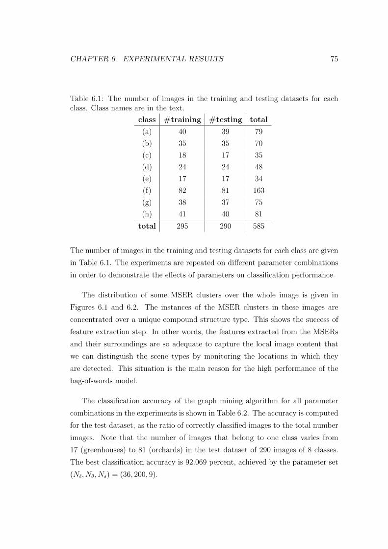
CHAPTER 6. EXPERIMENTAL RESULTS 75
Table 6.1: The number of images in the training and testing datasets for eachclass. Class names are in the text.
class #training #testing total
(a) 40 39 79
(b) 35 35 70
(c) 18 17 35
(d) 24 24 48
(e) 17 17 34
(f) 82 81 163
(g) 38 37 75
(h) 41 40 81
total 295 290 585
The number of images in the training and testing datasets for each class are given
in Table 6.1. The experiments are repeated on different parameter combinations
in order to demonstrate the effects of parameters on classification performance.
The distribution of some MSER clusters over the whole image is given in
Figures 6.1 and 6.2. The instances of the MSER clusters in these images are
concentrated over a unique compound structure type. This shows the success of
feature extraction step. In other words, the features extracted from the MSERs
and their surroundings are so adequate to capture the local image content that
we can distinguish the scene types by monitoring the locations in which they
are detected. This situation is the main reason for the high performance of the
bag-of-words model.
The classification accuracy of the graph mining algorithm for all parameter
combinations in the experiments is shown in Table 6.2. The accuracy is computed
for the test dataset, as the ratio of correctly classified images to the total number
images. Note that the number of images that belong to one class varies from
17 (greenhouses) to 81 (orchards) in the test dataset of 290 images of 8 classes.
The best classification accuracy is 92.069 percent, achieved by the parameter set
(N`, Nθ, Ns) = (36, 200, 9).

CHAPTER 6. EXPERIMENTAL RESULTS 76
Figure 6.1: Three clusters of stable dark MSERs are drawn with different colorsat ellipse centers for N` = 36. Yellow, green and magenta points are concentratedon dense residential areas with large buildings, dense residential areas with smallbuildings and orchards, respectively.

CHAPTER 6. EXPERIMENTAL RESULTS 77
Figure 6.2: Four clusters of different type MSERs are drawn with different colorsat ellipse centers for N` = 36. Yellow, green, cyan and magenta points areconcentrated on sea, forests, stream bed/clouds and dense residential areas withtrees, respectively.

CHAPTER 6. EXPERIMENTAL RESULTS 78
Tab
le6.
2:T
he
clas
sifica
tion
accu
racy
ofth
egr
aph
min
ing
algo
rith
m,
inp
erce
nta
ge(%
),fo
ral
lpar
amet
erse
tsin
the
exp
erim
ents
.
Num
ber
of
Subgra
phs
per
class
(Ns)
12
34
56
78
910
11
12
13
14
15
16
17
18
19
20
NumberofLabels(N`)
18
Nθ
200
8381
8187
8688
8687
8787
8686
8579
8382
8176
8178
500
7382
8583
8282
8886
8887
8887
8582
8279
7876
7574
800
6877
8284
8586
8687
8889
8887
8686
8484
8279
7576
26a
Nθ
200
7979
8287
8890
9189
8786
8589
8889
8888
8886
8684
500
7472
8483
8485
8681
8688
8887
8386
8483
8484
8381
800
7177
8183
8586
8887
8987
8785
8884
8283
7677
7575
36
Nθ
200
8078
8287
8990
9191
92
9090
9088
9188
9191
8985
84
500
8077
8785
8790
9089
8888
8988
8988
8787
7371
7369
800
7981
8786
8686
8688
8888
8784
8879
7685
7683
7169
54
Nθ
200
7377
8083
8889
8886
8988
8686
8687
8885
7880
6868
500
7479
8182
8284
8488
8788
8884
8172
8273
7669
6766
800
7277
7983
8585
8585
8481
8083
7978
7268
7467
6667
72
Nθ
200
7980
7983
8683
8682
8487
8481
8077
8173
7776
6471
500
7978
8080
8181
8082
8481
8180
8180
7672
6867
6562
800
7979
8184
8281
8081
7671
7177
7471
7068
7264
6160
aC
orre
spon
din
gcl
ust
erp
aram
eter
sis
Υ=
(4,4,9,9
)

CHAPTER 6. EXPERIMENTAL RESULTS 79
0 2 4 6 8 10 12 14 16 18 2060
65
70
75
80
85
90
Ns
Acc
urac
y
18 labels26 labels36 labels54 labels72 labels
Figure 6.3: Plot of classification accuracy of the graph mining algorithm for fivedifferent number of labels over the number of subgraphs per class. The lines aredrawn by averaging the accuracy values for the parameters Nθ ∈ 200, 500, 800.
Figure 6.3 demonstrates the effects of N` and Ns. Given these parame-
ters, the line is drawn by averaging the classification accuracy over the set
Nθ ∈ 200, 500, 800. If we start from Ns = 1 and increase the number of
subgraphs selected for the set S, i.e. the dimensionality of the feature space, the
classification accuracy also increases until about Ns = 8 or 10 for all values of
N`. However, after this point the classification accuracy decreases dramatically
as expected because of the curse of dimensionality. A similar behavior is observed
for the parameter N`. The best accuracy results are obtained when the number of
labels is 36. High number of node labels such as 72 causes a significant decrease
in subgraph frequency which leads to a fall in the accuracy. On the other hand,
small number of node labels like 18 increases the subgraph frequency but reduces
the correlation between subgraphs and classes. As a result, the confusion caused
by less correlated subgraphs results in low classification accuracy. To sum up,
every number of node labels entails trade-offs between frequency and correlation.
Finding the optimal number of node labels in terms of classification accuracy
requires experiments on the dataset with a range of N` values.

CHAPTER 6. EXPERIMENTAL RESULTS 80
Besides classification performance, the number of node labels plays an im-
portant role in computational complexity. The crucial part of the graph mining
algorithm with respect to the computational complexity is the frequent subgraph
mining. The computational cost depends heavily on the number of overlapping
embeddings because the MIS support solves an optimization problem for every
overlapping embeddings. Small number of labels increases the number of over-
lapping embeddings and some classes, especially natural lands such as forest,
fields and orchards tend to produce overlapping embeddings more than man-
made structures like residential areas.
Figure 6.4 demonstrates the effects of Nθ and Ns. Given these parame-
ters, the line is drawn by averaging the classification accuracy over the set
N` ∈ 18, 26, 36, 54, 72. The parameter Ns, namely the number of subgraphs
selected per class represents similar property as in Figure 6.3. On the other
hand, a decrease in the thresholds θ suppc and θ cor
c (inversely proportional to Nθ)
causes the classification accuracy to decrease. The analysis of this case is harder
than the previous. One possible explanation is that the set S contains strongly
correlated but less frequent subgraphs for low thresholds. The last part of the
mining algorithm uses the correlation function as a significance measure. There-
fore, the selected subgraphs may be still highly correlated despite the low corre-
lation threshold but they may be less frequent. For example, assume a pattern
π which is found once or twice in almost all examples of class c but not found in
other examples. The pattern π is considered to be a correlated pattern but it is
not frequent and may not be found in test examples. In summary, the last part of
the mining algorithm compensates a lower correlation threshold by selecting the
most correlated and not redundant pattern. Although the correlation measure
and pattern support are somewhat related (see Theorem 4.1), a lower threshold
for the subgraph support may not be fully recovered by the other parts. Conse-
quently, the selection of support threshold should be done carefully, that allows a
sufficient number of subgraphs to satisfy the frequency criterion considering the
redundancy between patterns.
The classification performance of the bag-of-words model in comparison to
the graph mining algorithm can be seen in Table 6.3. As seen in the table, the

CHAPTER 6. EXPERIMENTAL RESULTS 81
0 2 4 6 8 10 12 14 16 18 2060
65
70
75
80
85
90
Ns
Acc
urac
y
Nθ = 200
Nθ = 500
Nθ = 800
Figure 6.4: Plot of classification accuracy of the graph mining algorithm for threedifferent Nθ values over the number of subgraphs per class. The lines are drawnby averaging the accuracy values for the parameters N` ∈ 18, 26, 36, 54, 72.
frequency of visual words in the bag-of-words model is less affected from the num-
ber of node labels because the graph mining method seek structural elements in
the images. On the hand, bag-of-words model fails to classify images for small
number of node labels. The graph mining is less affected from the confusion using
the spatial relationships between local image patches. The best classification ac-
curacies of both methods are almost same. However, further improvement cannot
be obtained because of the intrinsic properties of the dataset. The small tile size
due to the heterogeneous content of the satellite image limits the frequency of the
subgraphs and the method suffers from the low subgraph support. Using bigger
tiles might improve the performance of the graph mining method.
The confusion matrices of the graph mining algorithm and the bag-of-words
models for the best parameter sets are presented in Figures 6.5 and 6.6, respec-
tively. The most confused class in both matrices is greenhouses. It is about
another problem of the dataset. Greenhouses are naturally located near sparse
residential areas (villages) and orchards. Therefore, the images of greenhouses

CHAPTER 6. EXPERIMENTAL RESULTS 82
Table 6.3: Classification accuracy of the bag-of-word model and the mining algo-rithm, in percentage terms, for different number of words/labels.
#Labels (N`) BoW Accuracy Max. Mining Accuracy
18 79.310 88.966 (Ns = 10, Nθ = 500)
26 92.414 91.034 (Ns = 7, Nθ = 200)
36 91.035 92.069 (Ns = 9, Nθ = 200)
54 91.035 88.621 (Ns = 9, Nθ = 200)
72 91.724 86.897 (Ns = 10, Nθ = 200)
in the dataset are not completely homogeneous and contain structures belonging
to other classes as seen in Figure 6.7. Our graph mining algorithm essentially
handles such problems by mining class correlated subgraphs. It seeks a set of
subgraphs which are commonly found among the examples of the class and some
images having other structures do not constitute an important problem for the
class. However, greenhouses are located sparsely in the Antalya image and almost
all greenhouse images contain structures of orchards or sparse residential areas.
As a result, the mining algorithm treats those structures as if they are correlated
with the greenhouses class. This explains the reason for the relatively lower per-
formance on the greenhouses and puts the obstacles in the way of improving the
general performance of the mining algorithm. Sample images for each class are
shown in Figure 6.7. They are grouped according to their classification result by
the graph mining algorithm.
Finally, we apply the SVM model learned from the training set to every tile
in the Antalya image. The classification result is drawn in Figure 6.8. Similarly,
we discover themes in the Antalya image using the LDA model whose parameters
are estimated from the training dataset for 12 themes. The set of subgraphs used
in the LDA model is the set S which is found by the graph mining algorithm.
The LDA model gives insight into distributions of themes over the whole image.
Hence, heterogeneous tiles contents are analyzed in a better manner. However,
presenting all topics distribution in this study for the Antalya image is a difficult
task. Therefore, we combine this distributions into one image in Figure 6.9 where
each color represents a region where the corresponding theme dominates other

CHAPTER 6. EXPERIMENTAL RESULTS 83
0.95
0.71
0.95
0.95
0.90
0.88
0.88
0.97
0.05
0.00.0
0.18
0.08
0.00.0
0.0
0.0 0.0 0.0 0.0 0.0 0.0
0.0 0.0 0.0 0.0 0.0
0.0 0.0 0.06
0.0 0.0 0.0 0.0
0.0 0.0 0.0
0.0 0.06
0.04
0.03
0.0 0.12
0.0 0.0 0.0 0.0 0.0
0.0 0.0 0.0 0.3 0.0 0.03
0.02 0.02
0.0
0.0 0.0 0.0 0.0 0.0 0.10 0.0
dense-large
orchards
greenhouses
sparse
dense-trees
dense-small
fields
forests
dens
e-lar
ge
orch
ards
gree
nhou
ses
spar
se
dens
e-tre
es
dens
e-sm
all
fields
fore
stsFigure 6.5: The confusion matrix of the graph mining algorithm using the param-eters N` = 36, Nθ = 200 and Ns = 9. Class names are given in short: sparse anddense are used for sparse and dense residential areas, respectively. Also, largeand small mean large and small buildings, respectively.
0.90
0.76
0.91
0.97
0.90
0.96
0.94
1.00
0.10
0.00.0
0.06
0.0
0.00.06
0.0
0.0 0.0 0.0 0.0 0.0 0.0
0.0 0.0 0.0 0.0 0.0
0.0 0.0 0.0
0.0 0.0 0.0 0.12
0.0 0.0 0.04
0.0 0.0
0.0
0.0
0.0 0.06
0.0 0.0 0.04 0.0 0.02
0.0 0.0 0.03 0.0 0.0 0.0
0.02 0.0
0.0
0.0 0.0 0.0 0.0 0.03 0.08 0.0
dense-large
orchards
greenhouses
sparse
dense-trees
dense-small
fields
forests
dens
e-lar
ge
orch
ards
gree
nhou
ses
spar
se
dens
e-tre
es
dens
e-sm
all
fields
fore
sts
Figure 6.6: The confusion matrix of the bag-of-words model for 26 labels. Classnames are given in short: sparse and dense are used for sparse and dense resi-dential areas, respectively. Also, large and small mean large and small buildings,respectively.

CHAPTER 6. EXPERIMENTAL RESULTS 84
(a) Correctly classified images (b) Misclassified images
Figure 6.7: Sample images from the dataset. The images at the left are correctlyclassified by the graph mining algorithm while the images at right-hand side aremisclassified using the parameters N` = 36, Nθ = 200 and Ns = 9. The imageclasses from top to down are in the order: dense residential areas with largebuildings, dense residential areas with small buildings, dense residential areaswith trees, sparse residential areas, greenhouses, orchards, forests and fields.

CHAPTER 6. EXPERIMENTAL RESULTS 85
Figure 6.8: The classification of all tiles except sea using the SVM learned fromthe training set for the parameters N` = 36, Nθ = 200 and Ns = 9. Each colorrepresents a unique class.
themes. The probability distributions of the most dominating 6 themes found
by the LDA model trained for 16 themes are drawn in Figure 6.10. The further
extensions of the LDA model remain as the future work for this study such as
theme localization by analyzing the locations where the correlated subgraphs are
found and testing with the model with other subgraph sets.

CHAPTER 6. EXPERIMENTAL RESULTS 86
Figure 6.9: Every tile is labeled by a unique color which indicates the correspond-ing theme that dominates the other themes in that tile. The theme distributionsare inferred from the LDA model for 12 themes. The subgraph set is the onemined in the previous experiments for the best parameters.

CHAPTER 6. EXPERIMENTAL RESULTS 87
Figure 6.10: The most dominating 6 themes are shown, found by the LDA modeltrained for 16 themes. The intensity of red color represents the probability of thetheme in an individual tile.

Chapter 7
Conclusions and Future Work
It would seem that perfection is attained
not when there is nothing more to add,
but when there is nothing left to take away.
“Wind, Sand and Stars” – Antoine de Saint-Exupery
7.1 Conclusions
We emphasized the importance of high-level understanding of the image content
through compound structures and we discussed the challenges of detecting com-
pound structures. Accordingly, we described a new image content representation
using the histogram of a subgraph set for classifying complex scenes such as dense
and sparse urban areas. As the first step of this method, we transformed images
to graphs where the nodes store local image content and the edges encode spatial
information. We proposed a graph construction method where the patches, en-
coded by the graph nodes, are detected using maximally extremal stable regions
and discriminative information about these regions are obtained by extracting
features from these regions in relation to their surroundings. The features were
quantized to form a codebook of local information that determined the node la-
bels and the neighborhood relation between local patches were found from the
88

CHAPTER 7. CONCLUSIONS AND FUTURE WORK 89
Voronoi tessellations of the patches.
In the second step of the method, we selected the subgraphs which are used
in the histogram representation of images where the subgraphs encapsulate the
local patches and their spatial arrangements within a specific structure. We
described a graph mining algorithm to find the set of frequent and discriminative
subgraphs which also has low redundancy. The algorithm first mines the frequent
subgraphs in the image graph set. Then, it selects the discriminative subgraphs
among the frequent ones with respect to the correlation between the subgraphs
and the classes. We introduced a novel algorithm for extracting class-correlated
patterns using the probabilistic model of subgraph frequency in an individual
graph. Finally, the redundancy between the subgraphs in the set was resolved by
choosing the most significant subgraphs considering the distances between them.
The third step of the method is the model learning from the vector space rep-
resentations of the images. A multi-class support vector machine was employed
for classifying the images. Furthermore, the latent Dirichlet allocation model
was used for further classification of images. The LDA model provides the theme
distribution representation of images computed from the subgraph histograms.
Themes provide a better understanding of the images having heterogeneous con-
tent.
In experimental work, we evaluated the performance of the graph mining al-
gorithm in image classification compared to the bag-of-words model. The dataset
consists of tiles cut from an Ikonos image of Antalya image and each tile is labeled
by one of the eight high-level semantic scene types. The classification accuracy
of the graph mining algorithm shows the effectiveness of the proposed method
in classification of complex scene types. We observed and discussed the effects
of the parameters on the classification accuracy. We concluded that the graph
mining algorithm is capable of discriminating images of different scene types suc-
cessfully. Furthermore, the LDA model manages to discover interesting themes
in the whole satellite image.

CHAPTER 7. CONCLUSIONS AND FUTURE WORK 90
7.2 Future Work
The proposed image representation can be easily adapted to other application
areas of computer vision. To illustrate, the application of subgraph histogram
representation can be extended to image retrieval by defining a distance measure
between subgraph histograms or borrowing a distance definition from the infor-
mation retrieval literature. Given an input image, the most similar images in the
dataset are the closest ones according to the distance function.
The LDA model offers new applications of the proposed image representation.
Given a given graph set and a subgraph set, the LDA model finds the subgraph-
theme probabilities β. A subgraph that is highly correlated with a theme can
be used for localizing the theme distribution in a heterogeneous content. This
enables high-level partitioning of heterogeneous images. Another application of
the LDA model is unsupervised partitioning of the whole satellite image using
subgraph histograms in case the labeled data are not available or the scene types
are unknown. In such cases, the subgraph set contains all subgraphs generated
by the graph language for a fixed-size. Given the number of themes, the LDA
tries to discover themes from the whole image using the occurrence numbers of
all subgraphs in tiles.
Finally, the set of subgraphs selected by the graph mining algorithm from an
Ikonos image of Antalya can be used for classification of images cut from another
satellite image which is retrieved from another satellite in a different spatial-
resolution, by the help of a mapping function. The function maps the features
extracted from the MSERs of the second image to the node labels determined
for the first image. The parameters of the graph construction method should be
adjusted for the spatial resolution of the second image, then the mapping function
determines, after normalization, the closest cluster center of the first image to the
features of an MSER in the second image.

Bibliography
[1] S. Aksoy. Modeling of remote sensing image content using attributed rela-
tional graphs. In D. Yeung, J. T. Kwok, A. Fred, F. Roli, and D. Ridder,
editors, Structural, Syntactic, and Statistical Pattern Recognition, volume
4109, chapter 52, pages 475–483. Springer Berlin Heidelberg, Berlin, Heidel-
berg, 2006.
[2] S. Aksoy. Signal and Image Processing for Remote Sensing, chapter Spatial
techniques for image classification, pages 491–513. Taylor & Francis, 2006.
[3] D. Arthur and S. Vassilvitskii. k-means++: the advantages of careful seed-
ing. In ACM-SIAM Symposium on Discrete Algorithms, pages 1027–1035,
Philadelphia, PA, USA, 2007. Society for Industrial and Applied Mathemat-
ics.
[4] E. Barbu, P. Hroux, S. Adam, and E. Trupin. Clustering document images
using graph summaries. In P. Perner and A. Imiya, editors, Machine Learning
and Data Mining in Pattern Recognition, volume 3587 of Lecture Notes in
Computer Science, pages 194–202. Springer, 2005.
[5] C. Berge. Hypergraphs. North-Holland Mathematical Library, 1989.
[6] J. Bilmes. A gentle tutorial of the em algorithm and its application to param-
eter estimation for gaussian mixture and hidden markov models. Technical
report, International Computer Science Institute, 1998.
[7] D. M. Blei, A. Y. Ng, and M. I. Jordan. Latent dirichlet allocation. Journal
of Machine Learning Research, 3:993–1022, 2003.
91

BIBLIOGRAPHY 92
[8] C. Borgelt. MoSS: Molecular substructure miner. http://www.borgelt.
net/moss.html, 2009.
[9] J. Bourgain. On lipschitz embedding of finite metric spaces in hilbert space.
Israel Journal of Mathematics, 52(1):46–52, March 1985.
[10] B. Bringmann. Mining Patterns in Structed Data. PhD thesis, Katholieke
Universiteit Leuven, Celestijnenlaan 200 A – B-3001 Leuven, Belgium, 2009.
[11] H. Bunke, P. Dickinson, M. Kraetzl, M. Neuhaus, and M. Stettler. Applied
Pattern Recognition, chapter Matching of Hypergraphs – Algorithms, Ap-
plications, and Experiments, pages 131–154. Springer Berlin / Heidelberg,
2008.
[12] H. Bunke and K. Riesen. Graph classification based on dissimilarity space
embedding. In Joint IAPR International Workshop on Structural, Syntac-
tic, and Statistical Pattern Recognition, pages 996–1007, Berlin, Heidelberg,
2008. Springer-Verlag.
[13] C.-C. Chang and C.-J. Lin. LIBSVM: a library for support vector machines,
2001. Software available at http://www.csie.ntu.edu.tw/~cjlin/libsvm.
[14] H. Cheng, X. Yan, J. Han, and C. wei Hsu. Discriminative frequent pattern
analysis for effective classification. In IEEE International Conference on
Data Engineering, pages 716–725, 2007.
[15] K. W. Church and W. A. Gale. Poisson mixtures. Natural Language Engi-
neering, 1:163–190, 1995.
[16] M. Deshpande, M. Kuramochi, N. Wale, and G. Karypis. Frequent
substructure-based approaches for classifying chemical compounds. IEEE
Transactions on Knowledge and Data Engineering, 17(8):1036 – 1050, aug.
2005.
[17] E. Dogrusoz and S. Aksoy. Modeling urban structures using graph-based
spatial patterns. In IEEE International Geoscience and Remote Sensing
Symposium, pages 4826 –4829, 23-28 2007.

BIBLIOGRAPHY 93
[18] M. Fiedler and C. Borgelt. Subgraph support in a single large graph. In
IEEE International Conference on Data Mining Workshops, pages 399–404,
Washington, DC, USA, 2007. IEEE Computer Society.
[19] R. Gaetano, G. Scarpa, and G. Poggi. Hierarchical texture-based segmenta-
tion of multiresolution remote-sensing images. IEEE Transactions on Geo-
science and Remote Sensing, 47(7):2129 –2141, july 2009.
[20] X. Gao, B. Xiao, D. Tao, and X. Li. Image categorization: Graph edit
distance+edge direction histogram. Pattern Recognition, 41(10):3179 – 3191,
2008.
[21] Z. Harchaoui and F. Bach. Image classification with segmentation graph
kernels. In IEEE Conference on Computer Vision and Pattern Recognition,
2007.
[22] G. Ivncsy, R. Ivncsy, and I. Vajk. Graph mining-based image indexing.
In International Symposium of Hungarian Researchers on Computational
Intelligence, pages 313–323, Budapest, Hungary, Nov 2004.
[23] H. Jiang and C. W. Ngo. Image mining using inexact maximal common sub-
graph of multiple args. In International Conference on Visual Information
Systems, 2003.
[24] Y. G. Jiang, J. Yang, C. W. Ngo, and A. G. Hauptmann. Representations of
keypoint-based semantic concept detection: A comprehensive study. IEEE
Transactions on Multimedia, 12(1):42–53, November 2009.
[25] M. Kuramochi and G. Karypis. Finding frequent patterns in a large sparse
graph. Data Mining and Knowledge Discovery, 11(3):243–271, 2005.
[26] S. Lazebnik, C. Schmid, and J. Ponce. Beyond bags of features: Spatial pyra-
mid matching for recognizing natural scene categories. In IEEE Conference
on Computer Vision and Pattern Recognition, volume 2, pages 2169–2178,
2006.

BIBLIOGRAPHY 94
[27] E. Levina and P. Bickel. The earth mover’s distance is the mallows distance:
some insights from statistics. In IEEE International Conference on Computer
Vision, volume 2, pages 251–256 vol.2, 2001.
[28] F.-F. Li and P. Perona. A bayesian hierarchical model for learning natural
scene categories. In IEEE Conference on Computer Vision and Pattern
Recognition, volume 2, pages 524–531, Washington, DC, USA, 2005. IEEE
Computer Society.
[29] T. Li, T. Mei, I.-S. Kweon, and X.-S. Hua. Contextual bag-of-words for
visual categorization. IEEE Transactions on Circuits and Systems for Video
Technology, PP(99):1 –1, Jan 2010.
[30] H. Mannila and H. Toivonen. Levelwise search and borders of theories in
knowledge discovery. Data Mining and Knowledge Discovery, 1(3):241–258,
1997.
[31] J. Matas, O. Chum, M. Urban, and T. Pajdla. Robust wide baseline stereo
from maximally stable extremal regions. In British Machine Vision Confer-
ence, 2002.
[32] R. Myers, R. Wison, and E. Hancock. Bayesian graph edit distance. IEEE
Transactions on Pattern Analysis and Machine Intelligence, 22(6):628 –635,
jun 2000.
[33] S. Nijssen, T. Guns, and L. De Raedt. Correlated itemset mining in roc
space: a constraint programming approach. In ACM SIGKDD International
Conference on Knowledge Discovery and Data Mining, pages 647–656, New
York, NY, USA, 2009. ACM.
[34] S. Nijssen and J. N. Kok. Multi-class correlated pattern mining. In Knowl-
edge Discovery in Inductive Databases, pages 165–187, 2005.
[35] S. Nowozin, K. Tsuda, T. Uno, T. Kudo, and G. H. Bakir. Weighted sub-
structure mining for image analysis. In IEEE Conference on Computer Vi-
sion and Pattern Recognition, 2007.
BIBLIOGRAPHY 95
[36] E. Pekalska and R. P. W. Duin. The Dissimilarity Representation for Pat-
tern Recognition: Foundations And Applications (Machine Perception and
Artificial Intelligence). World Scientific Publishing Co., Inc., River Edge,
NJ, USA, 2005.
[37] K. Riesen and H. Bunke. Iam graph database repository for graph based pat-
tern recognition and machine learning. In Joint IAPR International Work-
shop on Structural, Syntactic, and Statistical Pattern Recognition, pages 287–
297, Berlin, Heidelberg, 2008. Springer-Verlag.
[38] Y. Rubner, C. Tomasi, and L. J. Guibas. The earth mover’s distance as
a metric for image retrieval. International Journal of Computer Vision,
40(2):99–121, November 2000.
[39] G. Scarpa, R. Gaetano, M. Haindl, and J. Zerubia. Hierarchical multiple
markov chain model for unsupervised texture segmentation. IEEE Transac-
tions on Image Processing, 18(8):1830 –1843, aug. 2009.
[40] J. Sivic, B. C. Russell, A. A. Efros, A. Zisserman, and W. T. Freeman.
Discovering object categories in image collections. In IEEE International
Conference on Computer Vision, 2005.
[41] P. Soille. Morphological Image Analysis: Principles and Applications.
Springer-Verlag New York, Inc., Secaucus, NJ, USA, 2003.
[42] M. Stasolla and P. Gamba. Spatial indexes for the extraction of formal and
informal human settlements from high-resolution sar images. IEEE Jour-
nal of Selected Topics in Applied Earth Observations and Remote Sensing,
1(2):98 –106, june 2008.
[43] A. Vedaldi and B. Fulkerson. VLFeat: An open and portable library of
computer vision algorithms. http://www.vlfeat.org/, 2008.
[44] L. Vincent and E. Dougherty. Digital Image Processing Methods, chapter
Morphological Segmentation for Textures and Particles, pages 43–102. CRC,
1994.

BIBLIOGRAPHY 96
[45] D. Xin, Cheng, Hong, Yan, Xifeng, and J. Han. Extracting redundancy-
aware top-k patterns. In ACM SIGKDD International Conference on Knowl-
edge Discovery and Data Mining, pages 444–453, New York, NY, USA, 2006.
ACM.
[46] J. Yuan, Y. Wu, and M. Yang. Discovery of collocation patterns: from
visual words to visual phrases. In IEEE Conference on Computer Vision
and Pattern Recognition, pages 1 –8, Jun 2007.
[47] D. Zamalieva. Unsupervised detection of compound strctures using image
segmentation and graph-based texture analysis. Master’s thesis, Bilkent Uni-
versity, August 2009.