structural results on optimal transportation plans
TRANSCRIPT

Structural results on optimal transportation plans
by
Brendan Pass
A thesis submitted in conformity with the requirementsfor the degree of Doctor of PhilosophyGraduate Department of Mathematics
University of Toronto
Copyright c© 2011 by Brendan Pass

Abstract
Structural results on optimal transportation plans
Brendan Pass
Doctor of Philosophy
Graduate Department of Mathematics
University of Toronto
2011
In this thesis we prove several results on the structure of solutions to optimal transporta-
tion problems.
The second chapter represents joint work with Robert McCann and Micah Warren; the
main result is that, under a non-degeneracy condition on the cost function, the optimal
is concentrated on a n-dimensional Lipschitz submanifold of the product space. As a
consequence, we provide a simple, new proof that the optimal map satisfies a Jacobian
equation almost everywhere. In the third chapter, we prove an analogous result for the
multi-marginal optimal transportation problem; in this context, the dimension of the
support of the solution depends on the signatures of a 2m−1 vertex convex polytope of
semi-Riemannian metrics on the product space, induce by the cost function. In the fourth
chapter, we identify sufficient conditions under which the solution to the multi-marginal
problem is concentrated on the graph of a function over one of the marginals. In the fifth
chapter, we investigate the regularity of the optimal map when the dimensions of the two
spaces fail to coincide. We prove that a regularity theory can be developed only for very
special cost functions, in which case a quotient construction can be used to reduce the
problem to an optimal transport problem between spaces of equal dimension. The final
chapter applies the results of chapter 5 to the principal-agent problem in mathematical
economics when the space of types and the space of available goods differ. When the
dimension of the space of types exceeds the dimension of the space of goods, we show if
ii

the problem can be formulated as a maximization over a convex set, a quotient procedure
can reduce the problem to one where the two dimensions coincide. Analogous conditions
are investigated when the dimension of the space of goods exceeds that of the space of
types.
iii

Dedication
To Cristen
iv

Acknowledgements
I am deeply indebted to my thesis advisor, Robert McCann, for his patient guidance
and support. Working with Robert has been both enjoyable and extremely profitable for
me and I owe much of my development as a mathematician to him. This thesis could
certainly not have been completed without his help.
I gratefully acknowledge the help of my thesis committee members, Jim Colliander
and Bob Jerrard, as well as my external examiner Wilfrid Gangbo, all of whom provided
insightful suggestions and feedback on this work at various stages of its completion.
Stimulating discussions and useful remarks were also provided by Martial Agueh, Luigi
Ambrosio, Almut Burchard, Guillaume Carlier, Man-Duen Choi, Chandler Davis, Young-
Heon Kim, Paul Lee, Lars Stole and Micah Warren. The second chapter of this thesis
represents joint work with Robert McCann and Micah Warren.
It is a pleasure to thank the staff in the Department of Mathematics at the University
of Toronto, and in particular Ida Bulat, for helping make every aspect of my PhD run as
smoothly as possible. I am also grateful to all the friends and family members who lent
their support during the course of my degree.
Finally, I acknowledge that a refined version of Chapter 3 has been accepted for publi-
cation by Calculus of Variations and Partial Differential Equations, DOI : 10.1007/s00526-
011-0421-z.
v

Contents
1 Introduction 1
1.1 Background on optimal transportation . . . . . . . . . . . . . . . . . . . 1
1.2 Overview of Results . . . . . . . . . . . . . . . . . . . . . . . . . . . . . . 6
2 Rectifiability when m = 2 and n1 = n2. 13
2.1 Lipschitz rectifiability of optimal transportation plans . . . . . . . . . . . 14
2.2 Discussion and examples . . . . . . . . . . . . . . . . . . . . . . . . . . . 16
2.3 A Jacobian equation . . . . . . . . . . . . . . . . . . . . . . . . . . . . . 19
3 Quantified rectifiability for multi-marginal problems 22
3.1 Dimension of the support . . . . . . . . . . . . . . . . . . . . . . . . . . . 23
3.2 Examples . . . . . . . . . . . . . . . . . . . . . . . . . . . . . . . . . . . 29
3.2.1 Functions of the sum: c(x1, x2, ..., xm) = h(∑m
i=1 xi) . . . . . . . . 29
3.2.2 Hedonic pricing costs . . . . . . . . . . . . . . . . . . . . . . . . . 33
3.2.4 The determinant cost function . . . . . . . . . . . . . . . . . . . . 34
3.3 The Signature of g . . . . . . . . . . . . . . . . . . . . . . . . . . . . . . 35
3.4 Applications to the two marginal problem . . . . . . . . . . . . . . . . . 40
3.5 The 1-dimensional case: coordinate independence and a new proof of Car-
lier’s result . . . . . . . . . . . . . . . . . . . . . . . . . . . . . . . . . . . 41
4 Monge solutions and uniqueness for m ≥ 3 45
vi

4.1 Preliminaries and definitions . . . . . . . . . . . . . . . . . . . . . . . . . 45
4.2 Monge solutions . . . . . . . . . . . . . . . . . . . . . . . . . . . . . . . . 52
4.3 Examples . . . . . . . . . . . . . . . . . . . . . . . . . . . . . . . . . . . 56
5 Regularity of optimal maps when m = 2 and n1 6= n2. 62
5.1 Conditions and definitions . . . . . . . . . . . . . . . . . . . . . . . . . . 63
5.2 Regularity of optimal maps . . . . . . . . . . . . . . . . . . . . . . . . . 65
5.3 Regularity for non c-convex targets . . . . . . . . . . . . . . . . . . . . . 74
6 An application to the principal-agent problem 80
6.1 Assumptions and mathematical formulation . . . . . . . . . . . . . . . . 80
6.2 b-convexity of the space of products . . . . . . . . . . . . . . . . . . . . . 83
6.3 n1 > n2 . . . . . . . . . . . . . . . . . . . . . . . . . . . . . . . . . . . . 85
6.4 n2 > n1 . . . . . . . . . . . . . . . . . . . . . . . . . . . . . . . . . . . . 89
6.5 Conclusions . . . . . . . . . . . . . . . . . . . . . . . . . . . . . . . . . . 92
A Differential topology notation 93
Bibliography 95
vii
Chapter 1
Introduction
1.1 Background on optimal transportation
The optimal transportation problem asks what is the most efficient way to transform
one distribution of mass to another relative to a given cost function. The problem was
originally posed by Monge in 1781 [59]. In 1942, Kantorovich proposed a relaxed version
of the problem [41]; roughly speaking, he allowed a piece of mass to be split between two
or more target points. Since then, these problems have been studied extensively by many
authors and have found applications in such diverse fields as geometry, fluid mechanics,
statistics, economics, shape recognition, inequalities and meteorology.
Much of this thesis focuses on a multi-marginal generalization of the above; how do
we align m distributions of mass with maximal efficiency, again relative to a prescribed
cost function. Precisely, given Borel probability measures µi on smooth manifolds Mi of
respective dimensions ni, for i = 1, 2...,m and a continuous cost function c : M1 ×M2 ×
....×Mm → R, the multi-marginal version of Monge’s optimal transportation problem is
to minimize:
C(G2, G3, ..., Gm) :=
∫M1
c(x1, G2(x1), G3(x1), ..., Gm(x1))dµ1 (M)
among all (m − 1)-tuples of measurable maps (G2, G3, ..., Gm), where Gi : M1 → Mi
1

Chapter 1. Introduction 2
pushes µ1 forward to µi, G#µ1 = µi, for all i = 2, 3, ...,m. The Kantorovich formulation
of the multi-marginal optimal transportation problem is to minimize
C(µ) =
∫M1×M2...×Mm
c(x1, x2, ..., xm)dµ (K)
among all measures µ on M1 ×M2...×Mm which project to the µi under the canonical
projections; that is, for any Borel subset A ⊂Mi,
µ(M1 ×M2 × ....×Mi−1 × A×Mi+1....×Mm) = µi(A).
For any (m − 1)-tuple (G2, G3, ..., Gm) such that Gi#µ1 = µi for all i = 2, 3, ...,m,
we can define the measure µ = (Id,G2, G3, ..GM)#µ1 on M1 × M2 × ... × Mm, where
Id : M1 →M1 is the identity map. Then µ projects to µi for all i and C(G2, G3, ..., Gm) =
C(µ); therefore, K can be interpreted as a relaxed version of M. Roughly speaking,
the difference between the two formulations is that in M almost every point x1 ∈ M1
is coupled with exactly one point xi ∈ Mi for each i = 2, 3, ...,m, whereas in K an
element of mass at xi is allowed to be split between two or more target points in Mi for
i = 2, 3, ...,m. When m = 2, these are precisely the Monge and Kantorovich formulations
of the classical optimal transportation problem.
Under mild conditions, a minimizer µ for K will exist. Over the past two decades, a
great deal of research has been devoted to understanding the structure of these solutions.
When m = 2, under a regularity condition on µ1 and a twist condition on c, which we
will define subsequently, Levin showed that this solution is concentrated on the graph
of a function over x1, building on results of Gangbo [35], Gangbo and McCann [36] and
Caffarelli [14]. It is then straightforward to show that this function solves M and to
establish uniqueness results for both M and K. More recently, in the case where n1 = n2,
understanding the regularity, or smoothness, of the optimal map, has grown into an ac-
tive and exciting area of research, due to a major breakthrough by Ma, Trudinger and
Wang [52]. They identified a fourth order differential condition on c (called (A3s) in the
literature) which implies the smoothness of the optimizer, provided the marginals µ and

Chapter 1. Introduction 3
ν are smooth. Subsequent investigations by Trudinger and Wang [71, 70] revealed that
these results actually hold under a slight weakening of this condition, called (A3w), en-
compassing earlier results of Caffarelli [16][15][17], Urbas [72] and Delanoe [25, 26] when
c is the distance squared on either Rn or certain Riemannian manifolds, and Wang for an-
other special cost function [73]. Loeper [49] then verified that (A3w) is in fact necessary
for the solution to be continuous for arbitrary smooth marginals µ and ν. Loeper also
proved that, under (A3s), the optimizer is Holder continuous even for rougher marginals;
this result was subsequently improved by Liu [48], who found a sharp Holder exponent.
Since then, many interesting results about the regularity of optimal transportation have
been established [43][44][50][51][32][34][33][29][30].
A striking development in the theory of optimal transportation over the last 15 years
has been its interplay with geometry. Recently, the insight that intrinsic properties of
the solution µ, such as the regularity of Monge solutions, should not depend on the
coordinates used to represent the spaces has been very fruitful. The natural conclusion
is that understanding these properties is related to tensors, or coordinate independent
quantities. The relevant tensors encode information about the way that the cost function
and the manifolds interact. For example, Kim and McCann [43] introduced a pseudo-
Riemannian form on the product space, derived from the mixed second order partial
derivatives of the cost, whose sectional curvature is related to the regularity of Monge
solutions; they also noted that smooth solutions must be timelike for this form.
Whereas the two marginal problem is relatively well understood, results concerning
the structure of these optimal measures have thus far been elusive for m > 2. Much of the
progress to date has been in the special case where the Mi’s are all Euclidean domains of
common dimension n and the cost function is given by c(x1, x2, ..., xm) =∑
i 6=j |xi−xj|2,
or equivalently c(x1, x2, ..., xm) = −|(∑
i xi)|2. When n = 3, partial results for this cost
were obtained by Olkin and Rachev [62], Knott and Smith [45] and Ruschendorf and
Uckelmann [66], before Gangbo and Swiech proved that for a general m, under a mild

Chapter 1. Introduction 4
regularity condition on the first marginal, there is unique solution to the Kantorovich
problem and it is concentrated on the graph of a function over x1, hence inducing a
solution to a Monge type problem [37]; an alternate proof of Gangbo and Swiech’s theo-
rem was subsequently found by Ruschendorf and Uckelmann [67]. This result was then
extended by Heinich to cost functions of the form c(x1, x2, ..., xm) = h(∑
i xi) where h
is strictly concave [39] and, in the case when the domains Mi are all 1-dimensional, by
Carlier [19] to cost functions satisfying a strict 2-monotonicity condition. More recently,
Carlier and Nazaret [21] studied the related problem of maximizing the determinant (or
its absolute value) of the matrix whose columns are the elements x1, x2, ..., xn ∈ Rn; un-
like the results in [37],[39] and [19], the solution in this problem may not be concentrated
on the graph of a function over one of the xi’s and may not be unique. The proofs of
many of these results exploit a duality theorem, proved in the multi-marginal setting by
Kellerer [42]. Although this theorem holds for general cost functions, it alone says little
about the structure of the optimal measure; the proofs of each of the aforementioned
results rely heavily on the special forms of the cost.
The final chapter of this thesis focuses on the application of optimal transportation to
the principal-agent problem in economics. Problems of this type frequently in a variety
of different contexts in mathematical economic theory. The following formulation can be
found in Wilson [74], Armstrong [7] and Rochet and Chone [64]. A monopolist wants to
sell goods to a distribution of buyers. Knowing only the preference b(x, y) that a buyer
of type x ∈ X has for a good of type y ∈ Y , the density dµ(x) of the buyer types and
the cost c(y) to produce the good y, the monopolist must decide which goods to produce
and how much to charge for them in order to maximize her profits.
When the distribution of buyer types X and the available goods Y are either discrete
or 1-dimensional, this problem is well understood [69][58][61][8]. However, it is typically
more realistic to distinguish between both consumer types and goods by more than
one characteristic. An illuminating illustration of this is outlined by Figalli, Kim and
Chapter 1. Introduction 5
McCann [31]: consumers buying automobiles may differ by, for instance, their income
and the length of their daily commute, while the vehicles themselves may vary according
to their fuel efficiency, safety, comfort and engine power, for example. It is desirable,
then, to study models where the respective dimensions n1 and n2 of X and Y are greater
than 1 [53][63][65]. This multi-dimensional screening problem is much more difficult and
relatively little is known about it; for a review and an extensive list of references, see the
book by Basov [10].
When n1 = n2 and the preference function b(x, y) := x ·f(y) is linear in types, Rochet
and Chone [64]developed an algorithm for studying this problem. A key element in their
analysis is that, in this case, the problem may be formulated mathematically as an
optimization problem over the set of convex functions, which is itself a convex set. They
were then able to deduce the existence and uniqueness of an optimal pricing strategy, as
well as several interesting economic characteristics of it. Basov then analyzed the case
where b is linear in types but n1 6= n2 [9]. When n1 < n2, he was able to essentially reduce
the n2-dimensional space Y to an n1-dimensional space of artificial goods and then apply
the machinery of Rochet and Chone. When n1 > n2, no such reduction is possible in
general. Under additional hypotheses, however, he showed that the solution actually
coincides with the solution to a similar problem where both spaces are n1-dimensional.
For more general preference functions, Carlier, using tools from the theory of optimal
transportation, was able to formulate the problem as the maximization of a functional
P over a certain set of functions Ub,φ (a subset of the so called b-convex functions, which
will be defined below) [18]. He was then able to assert the existence of a solution to this
problem; that is, the existence of an optimal pricing schedule; an equivalent result is also
proven in [60]. However, for general functions b, the set of b-convex functions may not be
convex and so characterizing the solution using either computational or theoretical tools
is an extremely imposing task. Very little progress had been made in this direction until
recently, when Figalli, Kim and McCann [31] found necessary and sufficient conditions

Chapter 1. Introduction 6
on b for Ub,φ to be convex, assuming n1 = n2. Assuming in addition that the cost c is
b convex, they then demonstrated that the functional P is concave and from here were
able to prove uniqueness of the solution and demonstrate that some of the interesting
economic features observed by Rochet and Chone persist in this setting. Surprisingly, the
tools they use are also adapted from an optimal transportation context; their necessary
and sufficient condition is derived from a condition developed by Ma, Trudinger and
Wang [52], governing the regularity of optimal maps.
1.2 Overview of Results
This thesis consists of 6 chapters, including the introduction. The second chapter rep-
resents joint work with Robert McCann and Micah Warren and focuses on the case two
marginal problem when n1 = n2 := n. We study what can be said about the solution
under a certain non-degeneracy condition on the cost function, which was originally in-
troduced in an economic context by McAfee and McMillan [53] and later rediscovered
by Ma, Trudinger and Wang [52]; in the terminology of Ma, Trudinger and Wang, it is
also known as the (A2) condition. The main result is that, under this non-degeneracy
condition, the optimal measure concentrates on an n-dimensional, Lipschitz submanifold
of M1 ×M2 (see Theorem 2.0.2).
The proof of this theorem is based on an idea of Minty [57], which was also used by
Alberti and Ambrosio to show that the graph of any monotone function T : Rn → Rn is
contained in a Lipschitz graph over the diagonal ∆ = {u = x+y√2
: (x, y) ∈ Rn × Rn} [4].
The non-degeneracy condition can be viewed as a linearized version of the twist
condition, which asserts that the mapping y ∈ M− 7−→ Dxc(x, y) is injective. Under
suitable regularity conditions on the marginals, Levin [46] showed that the twist condition
ensures that the solution to the Kantorovich problem is concentrated on the graph of a
function and is therefore unique; see also Gangbo [35].
Chapter 1. Introduction 7
In one dimension, non-degeneracy implies twistedness, as was noted by many authors,
including Spence [69] and Mirrlees [58], in the economics literature; see also [56]. In
higher dimensions, this is no longer true; the non-degeneracy condition will imply that
the map y ∈ M− 7−→ Dxc(x, y) is injective locally but not necessarily globally. Non-
degeneracy was a hypothesis in the smoothness proof in [52], but does not seem to have
received much attention in higher dimensions before then. While our result demonstrates
that the non-degeneracy condition is enough to ensure that solutions still have certain
regularity properties, we will show by example that the uniqueness result that follows
from twistedness can fail for non-degenerate costs which are not twisted. The twist
condition is asymmetric in x and y; that is, there are cost functions for which the map
y ∈ M− 7−→ Dxc(x, y) is injective but x ∈ M+ 7−→ Dyc(x, y) is not. However, since
(D2xyc)
T = D2yxc the non-degeneracy condition is certainly symmetric in x and y. In view
of this, it is not surprising that the twist condition can only be used to show solutions are
concentrated on the graphs of functions of y over x whereas the non-degeneracy condition
implies solution are concentrated on n-dimensional submanifolds, a result that does not
favour either variable over the other.
Smooth optimal maps solve certain Monge-Ampere type equations. Typically, an
optimal map will be differentiable almost everywhere, but may not be smooth. It has
proven useful to know when non-smooth optimal maps solve the corresponding equa-
tions almost everywhere. Formally, the link between optimal transportation and these
equations was observed by Brenier [12], then Gangbo and McCann [36], and they were
studied in detail by Ma, Trudinger and Wang [52]. An important step in showing that
an optimal map solves a Monge-Ampere type equation is first showing that it solves the
Jacobian — or change of variables — equation. An injective Lipschitz function satisfies
the change of variables formula almost everywhere, so some sort of Lipschitz rectifiability
for the graphs of optimal maps is a useful tool in resolving this question. As an applica-
tion of Theorem 2.0.2, we provide a simple proof that optimal maps satisfy the change

Chapter 1. Introduction 8
of variables formula almost everywhere.
This work is related to another interesting line of research. A measure µ on the
product M+×M− is called simplicial if it is extremal among the convex set of all measures
which share its marginals. There are a number of results describing simplicial measures
and their supports [28][47][11][40][3]. One consequence is that the support of simplicial
measures are in some sense small; in particular, the support of a simplicial measure
on [0, 1] × [0, 1] must have two-dimensional Lebesgue measure zero [47][40]. Although
any measure supported on the graph of a function is simplicial, it is known that there
exist functions whose graphs have Hausdorff measure 2 − ε, for any ε > 0 [1]. For any
cost, the Kantorovich functional is linear and is hence minimized by some simplicial
measure. Conversely, any simplicial measure is the solution to a Kantorovich problem
for some continuous cost function, and so by the remarks above there are continuous cost
functions whose optimizers are supported on sets of Hausdorff dimension 2 − ε. On the
other hand, an immediate consequence of our result is that the support of optimizers of
Kantorovich problems with non-degenerate C2 costs have Hausdorff dimension at most
n, ie, at most one in this case.
The result of Ma, Trudinger and Wang proving smoothness of the optimal map under
certain conditions immediately implies that the support of the optimizer has Hausdorff
dimension n; however, the proof of this result requires that the marginals be C2 smooth.
Under the same assumptions on the cost functions but weaker regularity conditions on
the marginals, Loeper [49] and Liu [48] have demonstrated that the optimal map is
Holder continuous for some Holder constant 0 < α < 1. It is worth noting that there are
examples of functions on Rn [1] which are Holder continuous with exponent α but whose
graphs have Hausdorff dimension n + 1 − α, so the latter results do not imply that the
Hausdorff dimension of the optimizer must be n.
The third chapter applies similar techniques to the multi-marginal problem. Precisely,
we establish an upper bound on dim(spt(µ)). This bound depends on the cost function;

Chapter 1. Introduction 9
however, it will always be greater than or equal to the largest of the ni’s. In the case
when the ni’s are equal to some common value n, we identify conditions on c that ensure
our bound will be n and we show by example that when these conditions are violated,
the solution may be supported on a higher dimensional submanifold and may not be
unique. In fact, the costs in these examples satisfy naive multi-marginal extensions of
both the twist and non-degeneracy conditions; given the aforementioned results in the
two marginal case, we found it surprising that higher dimensional solutions can exist for
twisted, non-degenerate costs. On the other hand, if the support of at least one of the
measures µi has Hausdorff dimension n, the remarks above imply that spt(µ) must be
at least n dimensional; therefore, in cases where our upper bound is n, the support is
exactly n-dimensional, in which case we show it is actually n-rectifiable.
Unlike the results of Gangbo and Swiech, Heinich and Carlier, this contribution does
not rely on a dual formulation of the Kantorovich problem; instead, our method uses an
intuitive c-monotonicity condition to establish a geometrical framework for the problem.
The question about the dimension of spt(µ) should certainly have a coordinate indepen-
dent answer. Indeed, inspired partially by Kim and McCann, our condition is related
to a family of semi-Riemannian metrics1; heuristically, spt(µ) must be timelike for these
metrics and so their signatures control its dimension. From this perspective, the major
difference from the m = 2 case is that with two marginals, the metric of Kim and Mc-
Cann always has signature (n, n). In the multi-marginal case, there is an entire convex
family of relevant metrics, generated by 2m−1 − 1 extreme points, and their signatures
may vary depending on the cost.
Like the results in chapter 2 and in contrast to the results of Gangbo and Swiech [37],
Heinich [39], and Carlier [19], the results in chapter 3 only concern the local structure of
the optimizer µ and cannot be easily used to assert uniqueness of µ or the existence of a
1For the purposes of this paper, the term semi-Riemannian metric will refer to a symmetric, covariant2-tensor (which is not necessarily non-degenerate). The term pseudo-Riemannian metric will be reservedfor semi-Riemannian metrics which are also non-degenerate.
Chapter 1. Introduction 10
solution to M. On the other hand, we do explicitly exhibit fairly innocuous looking cost
functions which have high dimensional and non-unique solutions and so it is apparent
that these questions cannot be resolved in the affirmative without imposing stronger
conditions on c.
Question about Monge solutions and uniqueness are addressed in the fourth chapter.
We identify general conditions on c under which both K and M admit unique solutions,
generalizing the results of Gangbo and Swiech [37] and Heinich [39]. With one excep-
tion, the conditions we impose will look similar to standard conditions which arise when
studying the two marginal problem. Our lone novel hypothesis is that a certain covariant
2-tensor on the product space M2×M2× ...×Mm−1 should be negative definite. Whereas
the question about the dimension of the support of a solution µ to K is purely local,
showing that µ gives rise to a solution to M is a global issue: for almost all x1 ∈ M1
we must show that there is exactly one (x2, x3, ..., xm) ∈ M2 ×M3×, ...,Mm which get
coupled to x1 by µ. Our tensor here is designed to capture this global aspect of the
problem.
The fifth chapter focuses on the regularity theory of optimal maps when m = 2 but
n1 6= n2. A serious obstacle arises immediately; the regularity theory of Ma, Trudinger,
and Wang requires invertibility of the matrix of mixed second order partials ( ∂2c∂xi∂yj
)ij, and
its inverse appears explicitly in their formulations of (A3w) and (A3s). When m and n
fail to coincide, however, ( ∂2c∂xi∂yj
)ij clearly cannot be invertible. Alternate formulations
of the (A3w) and (A3s) that do not explicitly use this invertibility are known; however,
they rely instead on local surjectivity of the map y 7→ Dxc(x, y), which cannot hold in
our setting either.
Nonetheless, there is a certain class of costs for which our problem can easily be solved
using the results from the equal dimensional setting. Suppose
c(x, y) = b(Q(x), y), (1.1)
where Q : X → Z is smooth and Z is a smooth manifold of dimension n2. In this case,

Chapter 1. Introduction 11
it is not hard to show that the optimal map takes every point in each level set of Q to
a common y and studying its regularity amounts to studying an optimal transportation
problem on the n2-dimensional spaces Z and Y . We will show that costs of this form
are essentially the only costs on X × Y for which we can hope for regularity results
for arbitrary smooth marginals µ and ν. Indeed, for the quadratic cost on Euclidean
domains, the regularity theory of Caffarelli requires convexity of the target Y [16][15]
and, for general costs, it became apparent in the work of Ma, Trudinger and Wang [52]
that continuity of the optimizer cannot hold for arbitrary smooth marginals unless Y
satisfies an appropriate, generalized notion of convexity. Due to its dependence on the
cost function, this condition is referred to as c-convexity; when n1 > n2, we will show
that c-convexity necessarily fails unless the cost function is of the form alluded to above.
Given the preceding discussion, it is apparent that for cost functions that are not
of the special form (1.1), there are smooth marginals for which the optimal map is
discontinuous. However, as the condition (1.1) is so restrictive, it is natural to ask about
regularity for costs which are not of this form; any result in this direction will require
stronger conditions on the marginals than smoothness. In the final section of chapter 5,
we address this problem when n1 = 2 and n2 = 1.
In the sixth and final chapter, we turn our attention to the principal-agent problem.
Although the result of Figalli, Kim and McCann [31] represents major progress on this
problem, it is limited in that they had to assume that the spaces of types and products
were of the same dimension. There are many interesting and relevant economic models
in which these spaces have different dimensions, as in outlined in, for example, Basov
[10]. Our primary goal here is to study how the results in [31] extend to the case when
n1 6= n2; in particular, we want to determine under what conditions the set of b-convex
functions is convex for general values of n1 and n2. Our first contribution is to establish
a necessary condition for the convexity of this set. This condition, known as b-convexity
of Y , was a hypothesis in [31]; prior to that, to the best of my knowledge, it had not

Chapter 1. Introduction 12
been explored in the principal-agent context, although it is well known in the optimal
transportation literature since the work of Ma, Trudinger and Wang [52].
We then study separately the cases n1 > n2 and n1 < n2. The analysis here parallels
the work in chapter 5 on the regularity of optimal transportation between spaces whose
dimensions differ. When n1 > n2, we show that the b-convexity of Y implies that the
dimensions cannot differ in a meaningful way. That is, although b may appear to depend
on an n1 dimensional variable, there is a natural disintegration of X into smooth sub-
manifolds of dimension n1− n2 such that, no matter how the monopolist sets her prices,
types in the same sub-manifold always choose the same good. Therefore, types in the
same set are indistinguishable, and rather than working in an n1 dimensional space, we
may as well identify the types in a single sub-manifold and work instead in the resulting
n2 dimensional quotient space.
When n2 > n1, consumers’ marginal utilities cannot uniquely determine which prod-
uct they buy, making the problem largely intractable. In this case, given a price schedule,
a certain buyer’s surplus may be maximized by many different goods, making him in-
different between those goods. The monopolist’s profits will be very different, however,
depending on which good the buyer chooses. A naive possible solution would be to
only produce from the indifference set the good which maximizes the monopolist’s profit;
however, in doing this a good may be excluded which would maximize her profit from
another buyer. It turns out that the b-convexity on X (which was also an assumption
in [31]) precludes this from happening; under this condition, we can again reduce the
problem to one where the two spaces share the same dimension. A special case of this
result where b(x, y) = x · v(y) for a function v : Y 7→ Rn1 was established by Basov [9].

Chapter 2
Rectifiability when m = 2 and
n1 = n2.
This chapter represents joint work with Robert McCann and Micah Warren. We focus
on the two marginal problem when the dimensions n1 = n2 := n are equal and study the
local structure of the solution µ, assuming a non-degeneracy condition on c, which we
define below. For simplicity, throughout this chapter we will denote variables in M1 and
M2 by x and y, respectively, rather than x1 and x2.
In what follows, D2xyc(x0, y0) will denote the n by n matrix of mixed second order
partial derivatives of the function c at the point (x0, y0) ∈ M1 ×M2; its (i, j)th entry is
d2cdxidyj
(x0, y0).
Definition 2.0.1. Assume c ∈ C2(M1×M2). We say that c is non-degenerate at a point
(x0, y0) ∈M1 ×M2 if D2xyc(x0, y0) is nonsingular; that is if det(D2
xyc(x0, y0)) 6= 0.
For a probability measure µ on M1 ×M2 we will denote by spt(µ) the support of µ;
that is, the smallest closed set S ⊆M1 ×M2 such that µ(S) = 1.
Our main result is:
Theorem 2.0.2. Suppose c ∈ C2(M1 × M2) and µ1 and µ2 are compactly supported;
let µ be a solution of the Kantorovich problem. Suppose (x0, y0) ∈ spt(µ) and c is non-
13

Chapter 2. Rectifiability when m = 2 and n1 = n2. 14
degenerate at (x0, y0). Then there is a neighbourhood N of (x0, y0) such that N ∩ spt(µ)
is contained in an n-dimensional Lipschitz submanifold. In particular, if D2xyc is nonsin-
gular everywhere, spt(µ) is contained in an n-dimensional Lipschitz submanifold.
In the first section, we prove Theorem 2.0.2, while section 2.2 is devoted to discussion
and examples. In the final section we use Theorem 2.0.2 to provide a simple proof that
optimal maps satisfy a presrcribed Jacobian equation almost everywhere.
2.1 Lipschitz rectifiability of optimal transportation
plans
We now prove Theorem 2.0.2. Note that µ minimizes the Kantorovich functional if and
only if it maximizes the corresponding functional for b(x, y) = −c(x, y). To simplify the
computation, we consider µ that maximizes b.
Our proof relies on the b-monotonicity of the supports of optimal measures:
Definition 2.1.1. A subset S of M1×M2 is b-monotone if all (x0, y0), (x1, y1) ∈ S satisfy
b(x0, y0) + b(x1, y1) ≥ b(x0, y1) + b(x1, y0).
It is well known that the support of any optimizer is b-monotone [68], provided that
the cost is continuous and the marginals are compactly supported. The reason for this
is intuitively clear; if b(x0, y0) + b(x1, y1) < b(x0, y1) + b(x1, y0) then we could move some
mass from (x0, y0) and (x1, y1) to (x0, y1) and (x1, y0) without changing the marginals of
µ and thus increase the integral of b.
The strategy of our proof is to change coordinates so that locally b(x, y) = x·y, modulo
a small perturbation. We then switch to diagonal coordinates u = x + y, v = x− y and
show that the monotonicity condition becomes a Lipschitz condition for v as a function
of u. This trick dates back to Minty who used it to study monotone operators on Hilbert

Chapter 2. Rectifiability when m = 2 and n1 = n2. 15
spaces [57]; more recently, Alberti and Ambrosio used it to investigate the fine properties
of monotone functions on Rn [4].
We are now ready to prove Theorem 2.0.2:
Proof. Choose (x0, y0) in the support of µ. Fix local coordinates for M2 in a neighbour-
hood of y0 and set A := D2xyb(x0, y0). Then make the local change of coordinates y → Ay.
In these new coordinates, we have D2xyb(x0, y0) = I. We then have b(x, y) = x·y+G(x, y),
where D2xyG → 0 as (x, y) → (x0, y0). Set u
√2 = x + y and v
√2 = y − x. Given ε > 0,
choose a convex neighbourhood N of (x0, y0) such that ||D2xyG|| ≤ ε on N . We will
show that µ ∩ N is contained in a Lipschitz graph of v over u; hence, u and v serve as
local coordinates for our submanifold. Take (x, y) and (x′, y′) ∈ N ∩ sptµ. Then, by
b-monotonicity, we have b(x, y) + b(x′, y′) ≥ b(x, y′) + b(x′, y), hence
x · y +G(x, y) + x′ · y′ +G(x′, y′)
≥ x · y′ +G(x, y′) + x′ · y +G(x′, y).
Setting ∆x = x′ − x, ∆y = y′ − y, ∆u = u′ − u, ∆v = v′ − v, and rewriting yields
(∆x) · (∆y) + (∆x) ·∫ 1
0
∫ 1
0
D2xyG[x+ s∆x, y + t∆y](∆y)dsdt ≥ 0 (2.1)
which simplifies to: ∆x ·∆y ≥ −ε|∆x||∆y|.
Observe that ∆y√
2 = ∆u+ ∆v and ∆x√
2 = ∆u−∆v. Now,
|∆u|2 − |∆v|2 = 2(∆x) · (∆y)
≥ −2ε|∆x||∆y|
= −ε|∆u−∆v||∆u+ ∆v|
≥ −ε[|∆u|2 + |∆v|2]
The last inequality follows by squaring the absolute values of each side and expanding
the first term. Rearranging yields (1 + ε)|∆u|2 ≥ (1− ε)|∆v|2, the desired result.

Chapter 2. Rectifiability when m = 2 and n1 = n2. 16
Note that v may not be everywhere defined; that is, for certain values of u there
may be no corresponding v in spt(µ). However, the function v(u) can be extended by
Kirzbraun’s theorem and hence we can conclude that spt(µ) is contained in the graph of
a Lipschitz function of v over u.
Remark 2.1.1. Note that the only property of optimal transportation plans used in the
proof is b-monotonicity, so we have actually proven that any b-monotone subset of M1×
M2 is contained in an n-dimensional Lipschitz submanifold, provided b is non-degenerate.
2.2 Discussion and examples
For twisted costs, one can show that spt(µ) is concentrated on the graph of a function,
provided the marginal µ1 does not charge sets whose dimension is less than or equal to
n−1[35] [46] [52] [3] [55] [36]1; however, this can fail if µ1 charges small sets. On the other
hand, notice that our proof did not require any regularity hypotheses on the marginals.
In the example below, we exhibit a non-degenerate cost which is not twisted. We use
this example to illustrate how, in this setting, solutions may be supported on submani-
folds which are are not necessarily graphs. In addition, we show that these solutions may
not be unique. We can view this example as expressing an optimal transportation prob-
lem on a right circular cylinder via its universal cover, which is R2. The non-twistedness
of the cost and non-uniqueness of the solution arise because different points in the univer-
sal cover correspond to the same point in the cylinder and are therefore indistinguishable
by our cost function. In fact, if we expressed the problem on the cylinder, we would have
a twisted cost function and therefore a unique solution.
Example 2.2.1. Let M1 = M2 = R2 and c(x, y) = ex1+y1cos(x2− y2) + e2x
1
2+ e2y
1
2. Then
Dxc(x, y) = (ex1+y1cos(x2 − y2) + e2x
1,−ex1+y1sin(x2 − y2)), so y ∈ M2 7−→ Dxc(x, y) is
1In fact, this condition on the regularity of µ1 has recently been sharpened [38].

Chapter 2. Rectifiability when m = 2 and n1 = n2. 17
not injective and c is not twisted. However, note that D2xyc(x, y) = ex
1+y1cos(x2 − y2) ex1+y1sin(x2 − y2)
−ex1+y1sin(x2 − y2) ex1+y1cos(x2 − y2)
Therefore, detD2
xyc(x, y) = e2(x1+y1) > 0 for all (x, y), so c is non-degenerate. Optimal
measures for c, then, must be supported on 2-dimensional Lipschitz submanifolds, but we
will now exhibit an optimal measure whose support is not contained in the graph of a
function.
Now let M be the union of the three graphs:
G1 : y1 = x1, y2 = x2 + π (2.2)
G2 : y1 = x1, y2 = x2 + 3π (2.3)
G3 : y1 = x1, y2 = x2 + 5π (2.4)
Clearly, M is a smooth 2-d submanifold but not a graph. However, c(x, y) ≥ −ex1+y1 +
e2x1
2+ e2y
1
2≥ (ex
1−ey1 )22
and we have equality on M . Therefore, any probability measure
whose support is concentrated on M is optimal for its marginals.
We now show that optimal measures supported on M may not be unique. Let
S = {((x1, x2), (y1, y2))|0 ≤ x1 ≤ 1, 0 ≤ x2 ≤ 4π}
Note that
M ∩ S = (G1 ∩ S) ∪ (G2 ∩ S) ∪ (G3 ∩ S).
consists of 3, flat 2-d regions. Let µ be uniform measure on these regions. Now, let µ1
be uniform measure on the the first half of G1 ∩ S; that is, on
G1 ∩ {((x1, x2), (y1, y2))|0 ≤ x1 ≤ 1, 0 ≤ x2 ≤ 2π}.
Let µ3 be uniform measure on the the second half of G3 ∩ S, or
G3 ∩ {((x1, x2), (y1, y2))|0 ≤ x1 ≤ 1, 2π ≤ x2 ≤ 4π}.

Chapter 2. Rectifiability when m = 2 and n1 = n2. 18
Take µ2 to be twice uniform measure on G2 ∩ S and set µ = µ1+µ2+µ3. Then µ and
µ share the same marginals and are both optimal measures. Furthermore, any convex
combination tµ+ (1− t)µ will also share the same marginals and will be optimal as well.
The next example is similar in that the cost function is non-degenerate but not
twisted. However, this cost would be twisted if we exchanged the roles of x and y.
This demonstrates that, unlike non-degeneracy, the twist condition is not symmetric in
x and y. For this cost function, solutions will be unique as long as the second marginal
does not charge small sets.
Example 2.2.2. Let M1 = M2 = R2 and
c(x, y) = −(x1 cos(y1) + x2 sin(y1))ey2
+e2y
2
2+
(x1)2 + (x2)2
2.
Note that detD2xyc(x, y) = −e2y2 < 0, so c is non-degenerate. However, Dxc(x, y) =
(−cos(y1)ey2
+ x1,−sin(y1)ey2
+ x2), so y ∈ M2 7−→ Dxc(x, y) is not injective and c is
not twisted. On the other hand, Dyc(x, y) = ((x1sin(y1) + x2cos(y1))ey2,−(x1cos(y1) +
x2sin(y1))ey2+e2y
2) and so x ∈M1 7−→ Dyc(x, y) is injective. This implies that solutions
are supported on graphs of x over y but that these graphs are not necessarily invertible.
In fact, c(x, y) ≥ (((x1)2+(x2)2)12−ey2 )2
2≥ 0, where equality holds if and only if cos(y1) =
x1
((x1)2+(x2)2)12
, sin(y1) = x2
((x1)2+(x2)2)12
, and ((x1)2 + (x2)2)12 = ey
2. This set of equality is a
non-invertible graph of x over y; any measure whose support is contained in this graph is
optimal for its marginals. Note that as any minimizer for this problem must be supported
on this graph, the solution is unique [3].
Remark 2.2.3. For twisted costs with regular marginals, any solution is concentrated on
the graph of a particular function [52]. It is not hard to show that at most one measure
with prescribed marginals can be supported on such a graph; hence, uniqueness of the
optimizer follows immediately.
While our result asserts that for non-degenerate costs the solution concentrates on
some n-dimensional Lipschitz submanifold, the proof says little more about the subman-

Chapter 2. Rectifiability when m = 2 and n1 = n2. 19
ifold itself. In contrast to the twisted setting, then, our result cannot be used to deduce
a uniqueness argument. Furthermore, as Example 5.3.4 shows, even if we do know the
support of the optimizer explicitly, solutions may not be unique if this support is not
concentrated on the graph of a function.
Theorem 2.0.2 also says something about problems where D2xyc is allowed to be sin-
gular, but where the gradient of its determinant is non-zero at the singular points. In
this case, the implicit function theorem implies that the set where D2xyc is singular has
Hausdorff dimension 2n−1. Theorem 2.0.2 is valid wherever D2xyc is nonsingular, so that
the optimal measure is concentrated on the union of a smooth 2n − 1 dimensional set
and an n dimensional Lipschitz submanifold. For example, when n = 1, this shows that
the support of the optimal measure is 1-dimensional.
2.3 A Jacobian equation
We now provide a simple proof that an optimal map satisfies a prescribed Jacobian equa-
tion almost everywhere. This result was originally proven for the quadratic cost in Rn by
McCann [54], and for the quadratic cost on a Riemannian manifold by Cordero-Erasquin,
McCann and Schmuckenschlager [24]. Cordero-Erasquin generalized this approach to deal
with strictly convex costs on Rn [23]; see also [2]. It was observed by Ambrosio, Gigli
and Savare that this can be deduced from results in [5] and [6] when the optimal map is
approximately differentiable, which is true even for some non-smooth costs. Our method
works only when the cost is C2 and non-degenerate, but has the advantage of a simpler
proof, relying only on the area/coarea formula for Lipschitz functions.
For a Jacobian equation to make sense, the solution must be concentrated on the
graph of a function, and that function must be differentiable in some sense, at least
almost everywhere. A twisted cost suffices to ensure the first condition. The second
follows from the smoothness and non-degeneracy of c. Recall that for a twisted cost

Chapter 2. Rectifiability when m = 2 and n1 = n2. 20
the optimal map has the form T (x) = c-expx(Du(x)); as c-expx(·) is the inverse of
y 7−→ Dxc(x, y), its differentabiliy follows from the non-degeneracy of c and the inverse
function theorem. The almost everywhere differentiability of Du(x) (or, equivalently, the
almost everywhere twice differentiability of u) follows from C2 smoothness of c; u takes
the form u(x) =infy(c(x, y) − v(y)) for some function v(y) and is hence semi-concave
[36]. In the present context, we need only the weaker condition that the optimal map is
continuous almost everywhere; its differentiability will follow from Theorem 2.0.2.
Proposition 2.3.1. Assume that the cost is non-degenerate and that an optimizer µ
is supported on the graph of some function T : dom(T ) → M2 which is injective and
continuous when restricted to a set dom(T ) ⊆M1 of full Lebesgue measure. Suppose that
the marginals are absolutely continuous with respect to volume; set dµ1 = f+(x)dx and
dµ2 = f−(y)dy. Then, for almost every x, f+(x) = |detDT (x)|f−(T (x)).
Proof. Choose a point x where T is continuous and a neighbourhood U− of T (x) such
that for U+ = T−1(U−), the part of the optimal graph contained in U+ × U− lies in
a Lipschitz graph v = G(u) over the diagonal ∆ = {u = x+y√2
: (x, y) ∈ U+ × U−},
after a change of coordinates. Now x = u+v√2
and y = u−v√2
, so the optimal measure is sup-
ported on the graph of the Lipschitz function (x, y) = (F+(u), F−(u)) := (u+G(u)√2, u−G(u)√
2).
By projecting onto the diagonal, we obtain a measure ν on ∆ that pushes forward to
µ1|U+ and µ2|U− under the Lipschitz mappings F+ and F−, respectively. Now, as F+ is
Lipschitz, the image of any zero volume set must also have zero volume; as µ1|U+ is abso-
lutely continuous with respect to Lebesgue, ν must be as well; we will write ν = h(u)du.
Now, for almost every x ∈ U+ there is a unique y = T (x) such that (x, y) ∈ spt(µ)
and hence a unique u = x+y√2
on the diagonal such that x = F+(u). It follows that
the map F+ is one to one almost everywhere and so for every set A ⊆ ∆ we have∫Ah(u)du =
∫F+(A)
f+(x)dx. But the right hand side is∫Af+(F+(u))|detDF+(u)|du by
the area formula; as A was arbitrary, this means h(u) = f+(F+(u))|detDF+(u)| almost
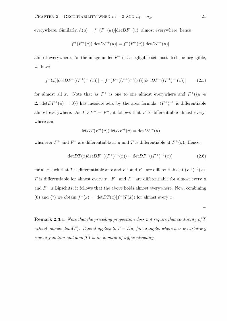
Chapter 2. Rectifiability when m = 2 and n1 = n2. 21
everywhere. Similarly, h(u) = f−(F−(u))|detDF−(u)| almost everywhere, hence
f+(F+(u))|detDF+(u)| = f−(F−(u))|detDF−(u)|
almost everywhere. As the image under F+ of a negligible set must itself be negligible,
we have
f+(x)|detDF+((F+)−1(x))| = f−(F−((F+)−1(x)))|detDF−((F+)−1(x))| (2.5)
for almost all x. Note that as F+ is one to one almost everywhere and F+({u ∈
∆ :detDF+(u) = 0}) has measure zero by the area formula, (F+)−1 is differentiable
almost everywhere. As T ◦ F+ = F−, it follows that T is differentiable almost every-
where and
detDT (F+(u))detDF+(u) = detDF−(u)
whenever F+ and F− are differentiable at u and T is differentiable at F+(u). Hence,
detDT (x)detDF+((F+)−1(x)) = detDF−((F+)−1(x)) (2.6)
for all x such that T is differentiable at x and F+ and F− are differentiable at (F+)−1(x).
T is differentiable for almost every x , F+ and F− are differentiable for almost every u
and F+ is Lipschitz; it follows that the above holds almost everywhere. Now, combining
(6) and (7) we obtain f+(x) = |detDT (x)|f−(T (x)) for almost every x.
Remark 2.3.1. Note that the preceding proposition does not require that continuity of T
extend outside dom(T ). Thus it applies to T = Du, for example, where u is an arbitrary
convex function and dom(T ) is its domain of differentiability.

Chapter 3
Quantified rectifiability for
multi-marginal problems
In this chapter, we prove an upper bound on the Hausdorff dimension of spt(µ) without
any restriction on m.
For a general m, there is an immediate lower bound on the Hausdorff dimension of
spt(µ); as spt(µ) projects to spt(µi) for all i, dim(spt(µ)) ≥ maxi(dim(spt(µi))). In the
present chapter, we establish an upper bound on dim(spt(µ)). This bound depends on
the cost function; however, it will always be greater than the largest of the ni’s. In
the case when the ni’s are equal to some common value n, we identify conditions on c
that ensure our bound will be n and we show by example that when these conditions
are violated, the solution may be supported on a higher dimensional submanifold and
may not be unique. In fact, the costs in these examples satisfy naive multi-marginal
extensions of both the twist and non-degeneracy conditions; given Theorem 2.0.2 and
the results in [46][35][36] and [14] outlined in the introduction, we found it surprising
that higher dimensional solutions can exist for twisted, non-degenerate costs. On the
other hand, if the support of at least one of the measures µi has Hausdorff dimension n,
the remarks above imply that spt(µ) must be at least n dimensional; therefore, in cases
22

Chapter 3. Quantified rectifiability for multi-marginal problems 23
where our upper bound is n, the support is exactly n-dimensional, in which case we show
it is actually n-rectifiable.
The chapter is organized as follows: in section 3.1, we state and prove our main result.
In section 3.2 we apply this result to several example cost functions. These include the
costs studied in [37][39] and [21] and we discuss how they fit into our framework. In
section 3.3, we discuss conditions that ensure the relevant metrics have only n timelike
directions, which will ensure spt(µ) is at most n-dimensional. In section 3.4, we discuss
some applications of our main result to the two marginal problem and in the final section
we take a closer look at the case when the marginals all have one dimensional support.
3.1 Dimension of the support
Before stating our main result, we must introduce some notation. Suppose that c ∈
C2(M1 ×M2 × ... ×Mm). Consider the set P of all partitions of the set {1, 2, 3, ...,m}
into 2 disjoint, nonempty subsets; note that P has 2m−1 − 1 elements. For any partition
p ∈ P , label the corresponding subsets p+ and p−; thus, p+ ∪ p− = {1, 2, 3, ...,m} and
p+ ∩ p− is empty. For each p ∈ P , define the following symmetric, bi-linear form on
M1 ×M2...×Mm
gp =∑
j∈p+,k∈p−
∂2c
∂xαjj ∂x
αkk
(dxαjj ⊗ dx
αkk + dxαkk ⊗ dx
αjj ) (3.1)
where, in accordance with the Einstein summation convention, summation on the αk
and αj is implicit. Here, the index αk ranges from 1 through nk and represents local
coordinates on Mk. Explicitly, given vectors v =⊕m
j=1 vαjj
∂
∂xαjj
and w =⊕m
j=1wαjj
∂
∂xαjj
we have
gp(v, w) =∑
j∈p+,k∈p−
∂2c
∂xαjj ∂x
αkk
(vαjj w
αkk + vαkk w
αjj )
Further details on this notation can be found in Appendix A.

Chapter 3. Quantified rectifiability for multi-marginal problems 24
Definition 3.1.1. We will say that a subset S of M1 ×M2 × ... ×Mm is c-monotone
with respect to a partition p if for all y = (y1, y2, ..., ym) and y = (y1, y2, ..., ym) in S we
have
c(y) + c(y) ≤ c(z) + c(z),
where
zi = yi and zi = yi, if i ∈ p+,
zi = yi and zi = yi, if i ∈ p−,
The following lemma, which is well known when m = 2, provides the link between
c-monotonicity and optimal transportation.
Lemma 3.1.2. Suppose µ is an optimizer and C(µ) < ∞. Then the support of µ is
c-monotone with respect to every partition p ∈ P .
Proof. Define Mp+ = ⊗i∈p+Mi and Mp− = ⊗i∈p−Mi. Note that we can identify M1 ×
M2 × ... ×Mm with Mp+ ×Mp− and let µp+ and µp− be the projections of µ onto Mp+
and Mp− respectively. Consider the two marginal problem
inf
∫Mp+×Mp−
c(x1, x2, ..., xm)dλ,
where the infinum is taken over all measures λ whose projections onto Mp+ and Mp− are
µp+ and µp− , respectively. Then µ is optimal for this problem and, as c is continuous, the
result follows from c-monotonicity for two marginal problems; see for example [68].
We will say a vector v ∈ T(x1,x2,...,xm)M1 ×M2 × ... ×Mm is spacelike (respectively
timelike or lightlike) for a semi-Riemannian metric g if g(v, v) ≥ 0 (respectively g(v, v) ≤
0 or g(v, v) = 0). We will say a subspace V ⊆ T(x1,x2,...,xm)M1 × M2 × ... × Mm is
spacelike (respectively timelike or lightlike) for g if every non-zero v ∈ V is spacelike
(respectively timelike or lightlike) for g. We will say V is strictly spacelike (respectively

Chapter 3. Quantified rectifiability for multi-marginal problems 25
strictly timelike) for g if no nonzero v ∈ V is timelike (respectively spacelike). We will
say a submanifold of T(x1,x2,...,xm)M1 ×M2 × ...×Mm is spacelike (respectively timelike,
lightlike, strictly spacelike or strictly timelike) at (x1, x2, ..., xm) if its tangent space at
(x1, x2, ..., xm) is spacelike (respectively timelike, lightlike, strictly spacelike or strictly
timelike).
We are now ready to state our main result:
Theorem 3.1.3. Let g be a convex combination of the gp’s defined in equation (3.1);
that is g =∑
p∈P tpgp where tp ≥ 0 for all p ∈ P and∑
p∈P tp = 1. Suppose µ is an
optimizer and C(µ) <∞; choose a point (x1, x2, ..., xm) ∈M1×M2× ...×Mm. Let N =∑mi=1 ni. Suppose the (+,−, 0) signature of g at (x1, x2, ..., xm) is (q+, q−, N − q+ − q−)
(ie, the corresponding matrix has q+ positive eigenvalues, q− negative eigenvalues and
a zero eigenvalue with multiplicity N − q+ − q−). Then there is a neighbourhood O of
(x1, x2, ..., xm) such that the intersection of the support of µ with O is contained in a
Lipschitz submanifold of dimension N − q+. Wherever the support is differentiable, it is
timelike for g.
Before we prove Theorem 3.1.3, a few remarks are in order. The theorem roughly says
that the dimension of spt(µ) is controlled by the signature of any convex combinations
of the gp’s; as these metrics may have very different signatures for different choices of
the tp’s, we are free to pick the one with the fewest timelike directions to give us the
best upper bound on the dimension of spt(µ) for a particular cost. When m = 2,
there is only one partition in P and consequently there is only one relevant metric,
∂2c∂xα11 ∂x
α22
(dxα11 ⊗ dxα2
2 + dxα22 ⊗ dxα1
1 ) in local coordinates. The matrix corresponding to
this metric is the block matrix studied by Kim and McCann [43]:
G =
0 D2x1x2
c
D2x2x1
c 0
.Here D2
xjxkc is the nj by nk matrix whose (αj, αk)th entry is ∂2c
∂xαjj ∂x
αkk
.

Chapter 3. Quantified rectifiability for multi-marginal problems 26
For m > 2, in the remainder of this paper we will focus primarily on the special case
when tp = 12m−1−1 for all p ∈ P . To distinguish it from the metrics obtained by other
convex combinations of the gp’s, we will denote the corresponding metric by g. Note that
the matrix of g in local coordinates is the block matrix given by
G =2m−2
2m−1 − 1
0 D2x1x2
c D2x1x3
c ... D2x1xm
c
D2x2x1
c 0 D2x2x3
c ... D2x2xm
c
D2x3x1
c D2x3x2
c 0 ... D2x3xm
c
... ... ... ... ...,
D2xmx1
c D2xmx2
c D2xmx3
c ... 0
.
Let us note, however, that other choices of the tp’s can give new and useful informa-
tion. For example, suppose we take tp to be 1 for a particular p and 0 for all others.
As in the proof of Lemma 2.2, we can identify M1 ×M2...×Mm = Mp+ ×Mp− , where
Mp± = ⊗j∈p±Mj and c(x1, x2, ..., xm) = c(xp+ , xp−) where xp± ∈ Mp± . In this case, G
will take the form:
G =
0 D2xp+xp−
c
D2xp−xp+
c 0
.The signature of this g is (r, r,N − 2r) where r is the rank of the matrix D2
xp+xp−c.
Letting np± =∑
j∈p± nj be the dimension of Mp± , we will have r ≤ min(np+ , np−). If it
is possible to choose a partition so that np+ = np− = N2
and D2xp+xp−
c has full rank, we
can conclude that spt(µ) is at most N2
dimensional. As we will see later, the number of
timelike directions for g may be very large and so this bound may in fact be better.
Our proof is an adaptation of our argument in chapter 2. When m = 2, after
choosing appropriate coordinates, we rotated the coordinate system and showed that
c-monotonicity implied that the solution was concentrated on a Lipschitz graph over
the diagonal, a trick dating back to Minty [57]. When passing to the multi-marginal
setting, however, it is not immediately clear how to choose coordinates that make an

Chapter 3. Quantified rectifiability for multi-marginal problems 27
analogous rotation possible; unlike in the two marginal case, it is not possible in general
to choose coordinates around a point (x1, x2, ..., xm) such that D2xixj
c(x1, x2, ..., xm) = I
for all i 6= j. The key to resolving this difficulty is the observation that Minty’s trick
amounts to diagonalizing the pseudo-metric of Kim and McCann and that this approach
generalizes to m ≥ 3.
Proof. Choose a point x = (x1, x2, ..., xm) ∈M1×M2×...×Mm . Choose local coordinates
around xi on each Mi and set Aij = D2xixj
c(x1, x2, ..., xm). For any ε > 0, there is a
neighbourhood O of (x1, x2, ..., xm) which is convex in these coordinates such that for all
(y1, y2, ..., ym) ∈ O we have ||Aij −D2xixj
c(y1, y2, ..., ym)|| ≤ ε, for all i 6= j.
Let G be the matrix of g at x in our chosen coordinates. There exists some invertible
N by N matrix U such that
UGUT = H :=
I 0 0
0 −I 0
0 0 0
,where the diagonal I, −I and 0 blocks have sizes determined by the signature of g.
Define new coordinates in O by u := Uy, where y = (y1, y2, ..., ym) and let u =
(u1, u2, u3) be the obvious decomposition. We will show that the optimizer is locally
contained in a Lipschitz graph in these coordinates.
Choose y = (y1, y2, ..., ym) and y = (y1, y2, ..., ym) in the intersection of spt(µ) and O.
Set ∆y = y − y. Set z = (z1, z2, ...zm) where
zi =
yi if i ∈ p+,
yi if i ∈ p−.
Similarly, set z = (z1, z2, ..., zm) where
zi =
yi if i ∈ p−,
yi if i ∈ p+.

Chapter 3. Quantified rectifiability for multi-marginal problems 28
Lemma 3.1.2 then implies
c(y) + c(y) ≤ c(z) + c(z)
or ∫ 1
0
∫ 1
0
∑j∈p+,i∈p−
(∆yi)TD2
xixjc(y(s, t))∆yjdtds ≤ 0,
where
yi(s, t) =
yi + s(∆yi) if i ∈ p+,
yi + t(∆yi) if i ∈ p−.
This implies that ∑j∈p+,i∈p−
(∆yi)TAij∆yj ≤ ε
∑j∈p+,i∈p−
|∆yi||∆yj|.
Hence, ∑p∈P
tp∑
j∈p+,i∈p−
(∆yi)TAij∆yj ≤ ε
∑p∈P
tp∑
j∈p+,i∈p−
|∆yi||∆yj|.
But this means
(∆y)TG∆y ≤ ε∑p∈P
tp∑
j∈p+,i∈p−
|∆yi||∆yj|. (3.2)
With ∆u = U∆y and ∆u = (∆u1,∆u2,∆u3) being the obvious decomposition, this
becomes:
|∆u1|2 − |∆u2|2 = (∆u)TH∆u = (∆y)TG∆y
≤ ε∑p∈P
tp∑
j∈p+,i∈p−
|∆yi||∆yj|
≤ εm2||U−1||23∑i
|∆ui|2,
where the last line follows because for each i and j we have
|∆yi||∆yj| ≤ |∆y|2
≤ ||U−1||2|∆u|2
= ||U−1||23∑i=1
|∆ui|2.

Chapter 3. Quantified rectifiability for multi-marginal problems 29
Choosing ε sufficiently small, we have
|∆u1|2 − |∆u2|2 ≤1
2
3∑i
|∆ui|2.
Rearranging yields
1
2|∆u1|2 ≤
3
2|∆u2|2 +
1
2|∆u3|2.
Together with Kirzbraun’s theorem, the above inequality implies that the support of µ
is locally contained in a Lipschitz graph of u1 over u2 and u3.
If spt(µ) is differentiable at x, the non-spacelike implication follows from taking y = x
in (3.2), then noting that we can take ε→ 0 as y → x.
3.2 Examples
In this section we apply Theorem 3.1.3 to several cost functions. Throughout this section,
we restrict our attention to the special semi-Riemannian metric g defined in the last
section.
3.2.1 Functions of the sum: c(x1, x2, ..., xm) = h(∑m
i=1 xi)
We first consider the case where Mi = Rn for all i and that c(x1, x2, ..., xm) = h(∑m
i=1 xi).
Proposition 3.2.1.1. Suppose Mi = Rn for all i and that c(x1, x2, ..., xm) = h(∑m
i=1 xi).
Denote the signature of D2h by (q+, q−, n − q+ − q−); then the signature of g is(q+ +
(m− 1)(q−), q− + (m− 1)q+,m(n− q+ − q−)).

Chapter 3. Quantified rectifiability for multi-marginal problems 30
Proof. Up to a positive, multiplicative constant, the matrix corresponding to g is
G =
0 D2h D2h ... D2h
D2h 0 D2h ... D2h
D2h D2h 0 ... D2h
... ... ... ... ...,
D2h D2h D2h ... 0
.
If v is an eigenvector of D2h with eigenvalue λ, then
[v, v, v, v...v, v]T
is an eigenvector of G with eigenvalue (m− 1)λ and
[v,−v, 0, 0, ..., 0]T , [v, 0,−v, 0, ..., 0]T , ..........................., [v, 0, 0, 0, ...,−v]T
are linearly independent eigenvectors with eigenvalue −λ. The result now follows easily.
Remark 3.2.1.2. When D2h is negative definite (corresponding to a uniformly concave
h), the signature of g reduces to ((m − 1)n, n, 0); combined with Theorem 3.1.3, this
implies that the support of any opimal measure µ is contained in an n-dimensional sub-
manifold. This is consistent with the results of Gangbo and Swiech[37] and Heinich[39],
who show that if the first marginal assigns measure zero to every set of Hausdorff dimen-
sion n− 1, then spt(µ) is contained in the graph of a function over x1.
On the other hand, when D2h is not negative definite, the signature of g has more than
n timelike directions. In this case, Theorem 3.1.3 does not preclude optimal measures
with higher dimensional supports. The next two results verify that this can in fact occur.
First we consider the extreme case, where h is uniformly convex; the signature of g
is then (n, (m− 1)n, 0).

Chapter 3. Quantified rectifiability for multi-marginal problems 31
Proposition 3.2.1.3. Suppose c(x1, x2, ..., xm) = h(∑m
i=1 xi), with D2h > 0. Then any
measure supported on the n(m− 1)- dimensional surface
S = {(x1, x2, ..., xm)|m∑i=1
xi = y},
where y ∈ Rn is any constant, is optimal for its marginals.
It should be noted that when m = 2, this surface is n dimensional.
Proof. Adding a function of the form∑m
i=1 ui(xi) to the cost c shifts the functional C(µ)
by an amount∑m
i=1
∫Miui(xi)dµi for each µ but does not change its minimizers. In
particular, minimizing the cost c is equivalent to minimizing
c′(x1, x2, ..., xm) := c(x1, x2, ..., xm)−m∑i=1
xi ·Dh(y) = f(m∑i=1
xi),
where f(z) := h(z) − z · Dh(y). Then f is a strictly convex function whose gradient
vanishes at z = y; it follows that y is the unique minimum of f . Hence, c′(x1, x2, ..., xm) ≤
f(y) with equality only when∑m
i=1 xi = y. It follows that any measure supported on S
is optimal for its marginals.
We now turn to the intermediate case where h has both concave and convex directions.
We show that there exist optimal measures whose supports have the maximal dimension
allowed by Theorem 3.1.3.
Proposition 3.2.1.4. Let c(x1, x2, ..., xm) = h(∑m
i=1 xi), where the signature of D2h is
(q, n − q, 0). Then there exist optimal measures whose support has dimension (n − q +
q(m− 1)).
Proof. At a fixed point p, we can add an affine function of (x1 + x2 + ... + xm) so that
Dh(p) = 0 and choose variables so that
D2h(p) =
I 0
0 −I
,

Chapter 3. Quantified rectifiability for multi-marginal problems 32
where the top left hand corner block is q by q and the bottom left hand corner block is
n− q by n− q. Then define the q-dimensional variables yi = (x1i , x2i , ..., x
qi ) and the n− q
dimensional variables zi = (xq+1i , xq+2
i , ..., xni ), so that h(∑m
i=1 xi) = h(∑m
i=1 yi,∑m
i=1 zi).
Now, near p, the implicit function theorem implies that for fixed zi, i = 1, 2, ...,m there
is a unique K = K(∑m
i=1 zi)), such that
Dyh(K(m∑i=1
zi),m∑i=1
zi) = 0
and K is smooth as a function of∑m
i=1 zi. As h is convex in it’s first slot near p,
h(K(m∑i=1
zi),m∑i=1
zi) ≤ h(m∑i=1
yi,
m∑i=1
zi)
for all nearby yi. Now, if we f(∑m
i=1 zi) = h(K(∑m
i=1 zi),∑m
i=1 zi) then f is a concave
function of∑m
i=1 zi. If we consider an optimal transportation problem for the zi with
cost f , the solution must be concentrated on a Lipschitz n− k dimensional submanifold.
Choose an n − q dimensional set S which supports an optimizer for this problem; by
considering a dual problem as in Gangbo and Swiech [37], we can find functions ui(zi)
such that f(∑m
i=1 zi) −∑m
i=1 ui(zi) ≥ 0 with equality if and only if (z1, z2, ...zm) ∈ S.
Therefore,
h(m∑i=1
yi,m∑i=1
zi))−m∑i=1
ui(zi) ≥ h(K(m∑i=1
zi),m∑i=1
zi)−m∑i=1
ui(zi) ≥ 0
and we have equality only when (z1, z2, ...zm) ∈ S and∑m
i=1 yi = K(∑m
i=1 zi), which is a
n− q + (m− 1)q dimensional set. It follows that this set is the support of an optimizer
for appropriate marginals.
Finally, we show that when the dimension of spt(µ) is larger than n, the solution may
not be unique.
Proposition 3.2.1.5. Set m = 4 and c(x, y, z, w) = h(x + y + z + w) for h strictly
convex. Suppose all four marginals µi are Lebesgue measure on the unit cube In in Rn.
Then the optimal measure is not unique.
Chapter 3. Quantified rectifiability for multi-marginal problems 33
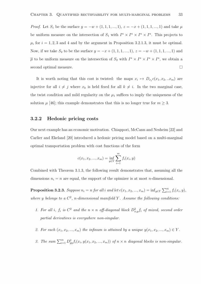
Proof. Let S1 be the surface y = −w + (1, 1, 1, ..., 1), z = −x + (1, 1, 1, ..., 1) and take µ
be uniform measure on the intersection of S1 with In × In × In × In. This projects to
µi for i = 1, 2, 3 and 4 and by the argument in Proposition 3.2.1.3, it must be optimal.
Now, if we take S2 to be the surface y = −x+ (1, 1, 1, ..., 1), z = −w + (1, 1, 1, ..., 1) and
µ to be uniform measure on the intersection of S2 with In × In × In × In, we obtain a
second optimal measure.
It is worth noting that this cost is twisted: the maps xi 7→ Dxjc(x1, x2, ..xm) are
injective for all i 6= j where xk is held fixed for all k 6= i. In the two marginal case,
the twist condition and mild regularity on the µ1 suffices to imply the uniqueness of the
solution µ [46]; this example demonstrates that this is no longer true for m ≥ 3.
3.2.2 Hedonic pricing costs
Our next example has an economic motivation. Chiappori, McCann and Nesheim [22] and
Carlier and Ekeland [20] introduced a hedonic pricing model based on a multi-marginal
optimal transportation problem with cost functions of the form
c(x1, x2, ..., xm) = infy∈Y
m∑i=1
fi(xi, y)
Combined with Theorem 3.1.3, the following result demonstrates that, assuming all the
dimensions ni = n are equal, the support of the opimizer is at most n-dimensional.
Proposition 3.2.3. Suppose ni = n for all i and let c(x1, x2, ..., xm) = infy∈Y∑m
i=1 fi(xi, y),
where y belongs to a C2, n-dimensional manifold Y . Assume the following conditions:
1. For all i, fi is C2 and the n × n off-diagonal block D2xiyfi of mixed, second order
partial derivatives is everywhere non-singular.
2. For each (x1, x2, ..., xm) the infinum is attained by a unique y(x1, x2, ..., xm) ∈ Y .
3. The sum∑m
i=1D2yyfi(xi, y(x1, x2, ..., xm)) of n× n diagonal blocks is non-singular.

Chapter 3. Quantified rectifiability for multi-marginal problems 34
Then the signature of g is ((m− 1)n, n, 0).
Proof. Fixing (x1, x2, ..., xm), we can choose coordinates so that
D2xiyfi(xi, y(x1, x2, ..., xm)) = I
for all i. Now,∑m
i=1Dyfi(xi, y(x1, x2, ..., xm)) = 0. SetM =∑m
i=1D2yyfi(xi, y(x1, x2, ..., xm))
and note that as M is non-singular by assumption we must have M > 0.. The implicit
function theorem now implies that y is differentiable with respect to each xj and:
m∑i=1
D2yyfi(xi, y(x1, x2, ..., xm))Dxjy(x1, x2, ..., xm) +D2
yxjfj(xi, y(x1, x2, ..., xm)) = 0.
So Dxjy(x1, x2, ..., xm) = −M−1. Now, as c(x1, x2, ..., xm) ≤∑m
i=1 fi(xi, y)) with equality
when y = y(x1, x2, ..., xm) we have
Dxic(x1, x2, ..., xm) = Dxif(xi, y(x1, x2, ..., xm)).
Differentiating with respect to xj yields
D2xixj
c(x1, x2, ..., xm) = Dxiyf(xi, y(x1, x2, ..., xm))Dxjy(x1, x2, ..., xm) = −M−1
for all i 6= j. The result now follows by the same argument as in Proposition 3.2.1.
3.2.4 The determinant cost function
Here we consider a problem studied by Carlier and Nazaret in [21], where the cost function
is −1 times the determinant; ie, for x1, x2, , ..., xn ∈ Rn, c(x1, x2, ..., xn) is −1 times the
determinant of the n by n matrix whose ith column is the vector xi. When n = 3, they
exhibit a specific example where the solution has 4-dimensional support; specifically, it’s
support is the set
S = {(x1, x2, x3) : |x1| = |x2| = |x3| and (x1, x2, x3)
forms a direct, orthogonal basis for R3}.
Although the signature of g varies for this cost, we show that on S it is (5, 4, 0).

Chapter 3. Quantified rectifiability for multi-marginal problems 35
Proposition 3.2.5. Assume c(x1, x2, x3) = −det(x1x2x3) and suppose (x1, x2, x3) forms
a direct, orthogonal basis for R3. Then the signature of g is (5, 4, 0).
Proof. Choose (x1, x2, x3) in the support; after applying a rotation we may assume x1 =
(|x1|, 0, 0), x2 = (0, |x1|, 0) and x3 = (0, 0, |x1|). A straightforward calculation then yields:
G = |x1|
0 0 0 0 −1 0 0 0 −1
0 0 0 1 0 0 0 0 0
0 0 0 0 0 0 1 0 0
0 1 0 0 0 0 0 0 0
−1 0 0 0 0 0 0 0 −1
0 0 0 0 0 0 0 1 0
0 0 1 0 0 0 0 0 0
0 0 0 0 0 1 0 0 0
−1 0 0 0 −1 0 0 0 0
.
There are 5 eigenvectors with eigenvalue 1:
[010100000]T , [001000100]T , [000001010]T , [1000-10000]T , [10000000-1]T .
There are 3 eigenvectors with eigenvalue -1:
[010-100000]T , [001000-100]T , [0000010-10]T .
Finally, there is a single eigenvector with eignenvalue -2:
[100010001]T
3.3 The Signature of g
This section is devoted to developing some results about the signature of the semi-metric
g =∑
p∈P tpgp at some point x = (x1, x2, ..., xm). Studying the signature at a point

Chapter 3. Quantified rectifiability for multi-marginal problems 36
reduces to understanding the matrix
g → G =
0 G12 G23 ... G1m
G21 0 G23 ... G2m
G31 G32 0 ... G3m
... ... ... ... ...,
Gm1 Gm2 Gm3 ... 0
. (3.3)
Here, for i 6= j,Gij = aijD2xixj
c where aij =∑tp and the sum is over all partitions
p ∈ P that separate i and j; that is, i ∈ p+ and j ∈ p− or i ∈ p− and j ∈ p+. Although
G is an N × N matrix, where N =∑m
i=1 ni, its signature can often be computed from
lower dimensional data, because of its special form. To illustrate this point, suppose
momentarily that the n′is are all equal to some common n and Gij’s are non-singular.
In this case, when m = 2 the signature of G will always be (n, n, 0) and, as we will see,
when m = 3 it is enough to calculate the signature of an appropriate n× n matrix.
One observation about the signature of the matrix G is immediate; as G has zero
blocks on the diagonal, it is possible to construct a lightlike subspace of dimension nmax =
maxi{ni}. This in turn implies that the number of spacelike directions can be no greater
than N − nmax; otherwise, it would be possible to construct a spacelike subspace of
dimension N−nmax+1, which would have to intersect non trivially with the null subspace.
Therefore, the best possible bound on the dimension of spt(µ) that Theorem 3.1.3 can
provide is nmax. This result is not too surprising. We have already noted that for suitable
marginals, the Hausdorff dimension of spt(µ) must be at least nmax; the discussion above
verifies that this is consistent with Theorem 3.1.3.
The first proposition gives an upper and lower bound for the number of timelike
directions.
Proposition 3.3.1. Let G be as in equation (3.3) and suppose rank(Gij) = r for some
i 6= j. Then the number of positive eigenvalues and the number of negative eigenvalues

Chapter 3. Quantified rectifiability for multi-marginal problems 37
of G are both at least r.
In particular, if ni = n for all i and Gij is invertible for some i 6= j, Theorem 3.1.3
implies that the support of any optimizer µ is at most (m− 1)n dimensional.
Proof. On the subspace TxiMi × TxjMj G restricts to 0 Gij
Gij 0
.NNote that (v, u) is a null vector if and only if u is in the null space of Gij and v is in
the nullspace of Gji. As these spaces are respectively ni − r and nj − r dimensional, the
nullspace of this matrix is ni + nj − 2r) dimensional.
As has been noted by Kim and McCann [43], the nonzero eigenvalues of this matrix
come in pairs of the form λ,−λ, with corresponding eigenvectors (v, u) and (v,−u),
respectively, where we take λ ≥ 0. Therefore, there are1
2(ni + nj − (ni + nj − 2r)) = r
positive eigenvalues and as many negative ones.
We can now construct a r dimensional timelike subspace for g. If q+ < r, then we
could construct a non-timelike subspace of dimension N − q+ > N − r (for example,
take the space spanned by all negative and null eigenvalues of G). These two spaces
would have to intersect non-trivially as their dimensions add to more than N , which is a
contradiction. An analagous argument applies to q−.
Next, we describe the signature in the m = 3 case:
Lemma 3.3.2. Suppose m = 3, for all i and that G23 in equation (3.3) is invertible. Set
A = G12(G32)−1G31; suppose A + AT has signature (r+, r−, n1 − r+ − r−). Then G has
signature (q+, q−,∑3
i=1 ni − q+ − q−) = (n2 + r−, n2 + r+, n1 − r+ − r−).
Proof. Note that the invertibility of G23 implies that n2 = n3. Consider the subspace
S = {(0, p, q) : p ∈ Tx2M2, q ∈ Tx3M3}.

Chapter 3. Quantified rectifiability for multi-marginal problems 38
By Proposition 3.3.1 we can find an orthonormal basis for this subspace consisting of n2
spacelike and n2 timelike directions. To determine the signature of g then, it suffices to
consider the restriction of g to the orthogonal complement (relative to g) S⊥ of S; any
orthonormal basis of S⊥ can be concatenated with a basis for S to form an orthonormal
basis for Tx1M1 × Tx2M2 × Tx3M3.
A simple calculation yields that S⊥ = {(v,−ATv,−Av) : v ∈ Tx1M1} and
(v,−ATv,−Av)TG(v,−ATv,−Av)) = −(A+ AT )(v, v),
which yields the desired result.
In particular, when ni = n for i = 1, 2, 3 and A is negative definite, g has signature
(2n, n, 0) and the support of any minimizer has dimension at most n.
A brief remark about Lemma 3.3.2 is in order. We mentioned in section 2 that, while
there is only one interesting pseudo metric when m = 2, there is an entire family of
metrics in the m ≥ 3 setting which may give new information about the behaviour of
spt(µ). However, when m = 3, ni = n for all i, D2xixj
c is non-singular for all i 6= j,
and the coefficients aij are all non zero, the signature of G is determined entirely by
A = G12(G32)−1G31 =
a12a31a32
D2x1x2
c(D2x3x2
c)−1D2x3x1
c. Choosing a different g simply
changes the aij’s, which does not effect the signature of A+AT . If one of the aij’s is zero,
it is easy to check that the signature of g must be (n, n, n); this yields a bound of 2n on
the dimension of spt(µ) which is no better than the bound obtained when all the aij’s
are non-zero. Thus, the only information about the dimension of spt(µ) which can be
provided by Theorem 3.1.3 is encoded in the bi-linear form D2x1x2
c(D2x3x2
c)−1D2x3x1
c(x)
on Tx1M1 × Tx1M1.
When m > 3, Lemma 3.3.2 easily yields the following necessary condition for the
signature of G to be ((m− 1)n, n, 0):
Corollary 3.3.3. Suppose ni = n for all i and the signature of G is ((m − 1)n, n, 0).
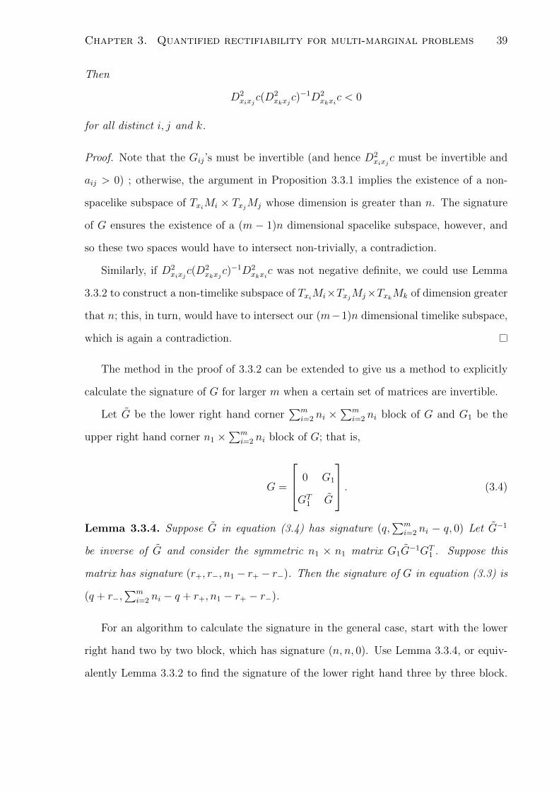
Chapter 3. Quantified rectifiability for multi-marginal problems 39
Then
D2xixj
c(D2xkxj
c)−1D2xkxi
c < 0
for all distinct i, j and k.
Proof. Note that the Gij’s must be invertible (and hence D2xixj
c must be invertible and
aij > 0) ; otherwise, the argument in Proposition 3.3.1 implies the existence of a non-
spacelike subspace of TxiMi × TxjMj whose dimension is greater than n. The signature
of G ensures the existence of a (m − 1)n dimensional spacelike subspace, however, and
so these two spaces would have to intersect non-trivially, a contradiction.
Similarly, if D2xixj
c(D2xkxj
c)−1D2xkxi
c was not negative definite, we could use Lemma
3.3.2 to construct a non-timelike subspace of TxiMi×TxjMj×TxkMk of dimension greater
that n; this, in turn, would have to intersect our (m−1)n dimensional timelike subspace,
which is again a contradiction.
The method in the proof of 3.3.2 can be extended to give us a method to explicitly
calculate the signature of G for larger m when a certain set of matrices are invertible.
Let G be the lower right hand corner∑m
i=2 ni ×∑m
i=2 ni block of G and G1 be the
upper right hand corner n1 ×∑m
i=2 ni block of G; that is,
G =
0 G1
GT1 G
. (3.4)
Lemma 3.3.4. Suppose G in equation (3.4) has signature (q,∑m
i=2 ni − q, 0) Let G−1
be inverse of G and consider the symmetric n1 × n1 matrix G1G−1GT
1 . Suppose this
matrix has signature (r+, r−, n1− r+− r−). Then the signature of G in equation (3.3) is
(q + r−,∑m
i=2 ni − q + r+, n1 − r+ − r−).
For an algorithm to calculate the signature in the general case, start with the lower
right hand two by two block, which has signature (n, n, 0). Use Lemma 3.3.4, or equiv-
alently Lemma 3.3.2 to find the signature of the lower right hand three by three block.

Chapter 3. Quantified rectifiability for multi-marginal problems 40
Then use Lemma 3.3.4 again to determine the signature of the lower right hand four by
four block and so on. After m− 1 applications of Lemma 3.3.4 we obtain the signature
of G.
3.4 Applications to the two marginal problem
We showed in chapter 2 that any solution to the two marginal problem was supported
on an n-dimensional Lipschitz submanifold, provided the marginals both live on smooth
n-dimensional manifolds and the cost is non-degenerate; that is, D2x1x2
c(x1, x2) seen as
a map from Tx1M1 to T ∗x2M2 is injective. Kim and McCann noted that in this case, the
signature of g is (n, n, 0) [43], so Theorem 3.1.3 immediately implies this result. In fact,
our analysis here is applicable to a larger class of two marginal problems, as in Theorem
3.1.3 we assumed neither non-degeneracy nor equality of the dimensions n1 and n2. If r is
the rank of the map D2x1x2
c(x1, x2), then the signature of g at (x1, x2) is (r, r, n1+n2−2r)
and so Theorem 3.1.3 yields the following corollary.
Corollary 1. Let m = 2 and r = rank(D2xixj
c) at some point (x1, x2). Then, near
(x1, x2), the support of any optimizer is contained in a Lipschitz manifold of dimension
n1 + n2 − r
It is worth noting that, even when n1 = n2, the topology of many important manifolds
prohibits the non-degeneracy condition from holding everywhere. Suppose, for example,
that M1 = M2 = S1, the unit circle. Then periodicity in x1 of ∂c∂x2
(x1, x2) implies
∫S1
∂2c
∂x1∂x2(x1, x2)dx1 = 0.
It follows that for every x2 there is at least one x1 such that ∂2c∂x1∂x2
(x1, x2) = 0. In chapter
2, we noted that under certain conditions the set where non-degeneracy fails is at most
(2n−1)-dimensional, which yields an immediate upper bound on the dimension of spt(µ).

Chapter 3. Quantified rectifiability for multi-marginal problems 41
Corollary 3.4 yields an improved bound; spt(µ) is at most 2n− r dimensional. A global
lower bound on r immediately yields an upper bound for the dimension of spt(µ).
Next we consider a two marginal problem where the dimensions of the spaces fail to
coincide; this type of problem has received very little attention in the literature. Suppose
n2 ≤ n1. If D2x1x2
c has full rank, ie, if r = n2 then this reduces to (n2, n2, n1−n2) and the
solution may have as many as n1 dimensions (in fact, if the support of the first marginal
has Hausdorff dimension n1, then the Hausdorff dimension of spt(µ) must be exactly n1).
This result has a nice heuristic explanation. To solve the problem, one would first solve
its dual problem, yielding two potential functions u1(x1) and u2(x2), and the solutions
lies in the set where the first order condition Du2(x2) = Dx2c(x1, x2) is satisfied. For a
fixed x2, this is a level set of the function x1 7→ Dx2c(x1, x2), which is generically n1−n2
dimensional. Fixing x2 and moving along this level set corresponds exactly to moving
along the null directions of g. On the other hand, as x2 varies, x1 must vary in such a
way so that the resulting tangent vectors are timelike. Hence, the solution may contain
all the lightlike directions of g, which correspond to fixing x2 and varying x1, plus n2
timelike directions, which correspond to varying x2 and with it x1.
3.5 The 1-dimensional case: coordinate independence
and a new proof of Carlier’s result
In [19], Carlier studied a multi-marginal problem where all the measures were supported
on the real line and proved that under a 2-monotonicity condition on the cost, the solution
must be one dimensional. To the best of our knowledge, this is the only result about the
multi-marginal problem proved to date that deals with a general class of cost functions.
The purpose of this section is to expose the relationship between 2-monotonicity and
the geometric framework developed in this paper. We will find an invariant form of this
condition and provide a new and simpler proof of Carlier’s result.

Chapter 3. Quantified rectifiability for multi-marginal problems 42
We begin with a definition:
Definition 3.5.1. We say c : Rm → R is i, j strictly 2-monotone with sign ±1 and write
sgn(c)ij = ±1 if for all x = (x1, x2, ..., xm) ∈ Rm and s, t > 0 we have
±[c(x) + c(x+ tei + sej)] < ±[c(x+ tei) + c(x+ sej)]
where (e1, e2, ...em) is the canonical basis for Rm.
In this notation, Carlier’s 2-monotonicity condition is that sgn(c)ij = −1 for all
i 6= j. This is not invariant under smooth changes of coordinates, however; the change
of coordinates xi 7→ −xi takes a cost with sgn(c)ij = −1 and transforms it to one with
sgn(c)ij = 1. However, it is easy to check that the following condition is coordinate
independent.
Definition 3.5.2. We say c is compatible if, for all distinct i, j, k we have
sgn(c)ijsgn(c)jksgn(c)ik
= −1.
It is also easy to check that c is compatible if and only if there exist smooth changes
of coordinates xi 7→ yi = fi(xi) for i = 1, 2, ...,m which transform c to a 2-monotone cost.
Combined with Carlier’s result, this observation implies that compatibility is sufficient
to ensure that the support of any optimizer is 1-dimensional.
If the cost is C2, the condition d2cdxidxj
< 0 is sufficient to ensure sgn(c)ij = −1; likewise,
d2cdxidxj
( d2cdxkdxj
)−1 d2cdxidxk
< 0 ensures that c is compatible. We can think of the condition on
the threefold products D2x1x2
c(D2x3x2
c)−1D2x3x1
c in Lemma 3.3.2 as a multi-dimensional,
coordinate independent version of Carlier’s condition. Corollary 3.3.3 demonstrates that
this condition is necessary for g to have signature ((m − 1)n, n, 0) and, when m = 3,
Lemma 3.3.2 shows that it is also sufficient. For m > 3, however, it is not sufficient even
in one dimension. As a counterexample, consider the cost function
c(x1, x2, x3, x4) = −x1x2 − x1x3 − x1x4 − x2x3 − x2x4 − 5x3x4.

Chapter 3. Quantified rectifiability for multi-marginal problems 43
For this cost,
G = −
0 1 1 1
1 0 1 1
1 1 0 5
1 0 5 0
,
which has signature (2, 2, 0)
Thus, Theorem 3.1.3 implies neither Carlier’s result nor the generalization above ,
at least if we restrict our attention to the special metric g. Below, we reconcile this by
providing a new proof of Carlier’s result, with the slightly stronger assumption d2cdxidxj
< 0
in place of 2-monotonicity.
We call a set S ⊆ R2 non-decreasing if (x− x)(y− y) ≥ 0 whenever (x, y), (x, y) ⊆ S.
The crux of Carlier’s argument is the following result:
Theorem 3.5.3. Suppose d2cdxidxj
< 0 for all i 6= j . Then the projections of the support
of the optimizer onto the planes spanned by x1 and xj are non-decreasing subsets for all
j.
In view of the preceding remarks, this implies that when the cost has negative three-
fold products d2cdxidxj
( d2cdxkdxj
)−1 d2cdxidxk
, the support is 1-dimensional.
Carlier’s proof relies heavily on duality. He shows that he can reduce the problem to a
series of two marginal problems with costs derived from the solution to the dual problem.
He then shows that these cost inherit monotonicity from c and hence their solutions
are concentrated on monotone sets. We provide a simple proof that uses only the c-
monotonicity of the support. In addition, our proof does not require any compactness
assumptions on the supports of the measures. However, after establishing this result, it
is not hard to show that, if the first measure is nonatomic, the support is concentrated
on the graph of a function over x1.
Morally, our proof applies the non-spacelike conclusion of Theorem 3.1.3 to a well
chosen semi-metric; however, because we don’t know a priori that the optimizer is smooth

Chapter 3. Quantified rectifiability for multi-marginal problems 44
we will prove the theorem directly from c-monotonicity.
Proof. Suppose (x1, ..., xm) and (y1, ..., ym) belong to the support of the optimizer. We
want to show (x1 − y1)(xi − yi) ≥ 0 for all i. If not, we may assume without loss of
generality that for some 2 ≤ k ≤ m we have (x1 − y1)(xi − yi) ≥ 0 for all i < k and
(x1− y1)(xi− yi) < 0 for i ≥ k. Hence, (xj − yj)(xi− yi) ≤ 0 for all j < k and i ≥ k. By
c-monotonicity, we have
c(x1, ..., xm) + c(y1, ..., ym) ≤ c(y1, ..., yk−1, xk, ..., xm) + c(x1, ..., xk−1, yk, ..., ym).
Hence,
k−1∑i=1
m∑j=k
(xi − yi)(xj − yj)∫ 1
0
∫ 1
0
d2c
dxidxj(y1(t), y2(t), ..., yk−1(t), yk(s), ..., ym(s))dtds
≤ 0
where yi(t) = yi + t(xi − yi) for i = 1, 2, ..k − 1 and yj(s) = yj + s(xj − yj) for j =
k, k + 1, ...,m. But, as d2
dxidxjc(y1(t), y2(t), ..., yk − 1(t), yk(s), ..., ym(s)) < 0, and (xi −
yi)(xj − yj) ≤ 0 for all i < k and j ≥ k, every term in the sum is nonnegative. As
(x1 − y1)(xj − yj) < 0 for j ≥ k, the sum must be positive, a contradiction.

Chapter 4
Monge solutions and uniqueness for
m ≥ 3
Our aim in this chapter is to establish necessary conditions on c under which M admits
a solution; this amounts to showing that the solution µ to K is concentrated on the
graph of a function over x1. We will then demonstrate that, under these conditions, the
solutions to M and K are both unique.
In the first section we formulate the conditions we will need. In section 4.2 we state
and prove our main result and in the third section we exhibit several examples of cost
functions which satisfy the criteria of our main theorem.
Throughout this chaper, we will assume the dimensions ni are all equal and denote
their common value by n.
4.1 Preliminaries and definitions
We will assume that each Mi can be smoothly embedded in some larger manifold in
which its closure Mi is compact and that the cost c ∈ C2(M1 × M2 × ... × Mm). In
addition, we will assume that Mi is a Riemannian manifold for i = 2, 3, ..m− 1 and that
45
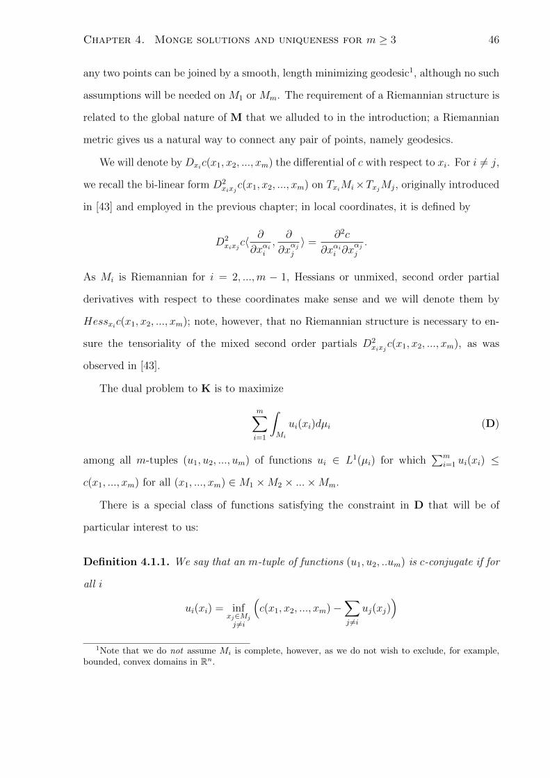
Chapter 4. Monge solutions and uniqueness for m ≥ 3 46
any two points can be joined by a smooth, length minimizing geodesic1, although no such
assumptions will be needed on M1 or Mm. The requirement of a Riemannian structure is
related to the global nature of M that we alluded to in the introduction; a Riemannian
metric gives us a natural way to connect any pair of points, namely geodesics.
We will denote by Dxic(x1, x2, ..., xm) the differential of c with respect to xi. For i 6= j,
we recall the bi-linear form D2xixj
c(x1, x2, ..., xm) on TxiMi×TxjMj, originally introduced
in [43] and employed in the previous chapter; in local coordinates, it is defined by
D2xixj
c〈 ∂
∂xαii,∂
∂xαjj
〉 =∂2c
∂xαii ∂xαjj
.
As Mi is Riemannian for i = 2, ...,m − 1, Hessians or unmixed, second order partial
derivatives with respect to these coordinates make sense and we will denote them by
Hessxic(x1, x2, ..., xm); note, however, that no Riemannian structure is necessary to en-
sure the tensoriality of the mixed second order partials D2xixj
c(x1, x2, ..., xm), as was
observed in [43].
The dual problem to K is to maximize
m∑i=1
∫Mi
ui(xi)dµi (D)
among all m-tuples (u1, u2, ..., um) of functions ui ∈ L1(µi) for which∑m
i=1 ui(xi) ≤
c(x1, ..., xm) for all (x1, ..., xm) ∈M1 ×M2 × ...×Mm.
There is a special class of functions satisfying the constraint in D that will be of
particular interest to us:
Definition 4.1.1. We say that an m-tuple of functions (u1, u2, ..um) is c-conjugate if for
all i
ui(xi) = infxj∈Mj
j 6=i
(c(x1, x2, ..., xm)−
∑j 6=i
uj(xj))
1Note that we do not assume Mi is complete, however, as we do not wish to exclude, for example,bounded, convex domains in Rn.
Chapter 4. Monge solutions and uniqueness for m ≥ 3 47
Whenever (u1, u2, ..um) is c-conjugate, the ui are semi-concave and hence have super
differentials ∂ui(xi) at each point xi ∈ Mi. By compactness, for each xi ∈ Mi we can
find xj ∈ Mj for all j 6= i such that u(xi) = c(x1, x2, ..., xm)−∑
j 6=i uj(xj); furthermore,
as long as |ui(xi)| <∞ for at least one xi, ui is locally Lipschitz [54].
The following theorem makes explicit the link between the Kantorovich problem and
its dual.
Theorem 4.1.1. There exists a solution µ to the Kantorovich problem and a c-conjugate
solution (u1, u2, ..., um) to its dual. Furthermore, the maximum value in D coincides with
the minimum value in K. Finally, for any solution µ to K, any c-conjugate solution
(u1, u2, ..., um) to D and any (x1, ..., xm) ∈ spt(µ) we have∑m
i=1 ui(xi) = c(x1, ..., xm).
This result is well known in the two marginal case; for m ≥ 3, the existence of
solutions to K and D as well as the equality of their extremal values was proved in [42].
The remaining conclusions were proved for a special cost by Gangbo and Swiech [37]
and for a general, continuous cost when each Mi = Rn by Carlier and Nazaret [21]. The
same proof applies for more general spaces Mi; we reproduce it below in the interest of
completeness.
Proof. As mentioned above, a proof of the existence of solutions µ to K and (v1, v2, ..., vm)
to D as well as the equality:
m∑i=1
∫Mi
vi(xi)dµi =
∫M1×M2....×Mm
c(x1, x2, x3, ..., xm)dµ (4.1)
can be found in [42]. We use a convexification trick, also found in [37] and [21], to build
a c-conjugate solution to D.
Define
u1(x1) = infxj∈Mj
j≥2
(c(x1, x2, ..., xm)−
m∑j=2
vj(xj))
and ui inductively by
ui(xi) = infxj∈Mj
j 6=i
(c(x1, x2, ..., xm)−
i−1∑j=1
uj(xj)−m∑
j=i+1
vj(xj))
Chapter 4. Monge solutions and uniqueness for m ≥ 3 48
As
um(xm) = infxj∈Mj
j 6=i
(c(x1, x2, ..., xm)−
m−1∑j=1
uj(xj)),
we immediately obtain
ui(xi) ≤ infxj∈Mj
j 6=i
(c(x1, x2, ..., xm)−
∑j 6=i
uj(xj)). (4.2)
The definition of ui−1 implies that for all (x1, x2, ...xm)
vi(xi) ≤ c(x1, x2, ..., xm)−i−1∑j=1
uj(xj)−m∑
j=i+1
vj(xj)
Therefore, vi(xi) ≤ ui(xi). It then follows that
ui(xi) = infxj∈Mj
j 6=i
(c(x1, x2, ..., xm)−
i−1∑j=1
uj(xj)−m∑
j=i+1
vj(xj))
≥ infxj∈Mj
j 6=i
(c(x1, x2, ..., xm)−
∑j 6=i
uj(xj)),
which, together with (4.2), implies that (u1, u2, ..., um) is c-conjugate. Now, we have
m∑i=1
∫Mi
vi(xi)dµi ≤m∑i=1
∫Mi
ui(xi)dµi
=m∑i=1
∫M1×M2....×Mm
ui(xi)dµ
≤∫M1×M2....×Mm
c(x1, x2, x3, ..., xm)dµ
and so by (4.1) we must have
m∑i=1
∫Mi
ui(xi)dµi =m∑i=1
∫M1×M2....×Mm
ui(xi)dµ =
∫M1×M2....×Mm
c(x1, x2, x3, ..., xm)dµ
But because∑m
i=1 ui(xi) ≤ c(x1, x2, x3, ..., xm), we must have equality µ almost ev-
erywhere. Continuity then implies equality holds on spt(µ).

Chapter 4. Monge solutions and uniqueness for m ≥ 3 49
As a corollary to the duality theorem, we now prove a uniqueness result for the
solution to D. When m = 2, this result, under the weak conditions on c stated below, is
due to Chiappori, McCann and Nesheim [22]; for certain special, multi-marginal costs,
it was proven by Gangbo and Swiech [37] and Carlier and Nazaret [21]. Although this
result is tangential to the main goals of this chapter, we prove it here to emphasize that,
whereas uniqueness in K requires certain structure conditions on the cost, uniqueness in
D depends only on the differentiability of c.
Corollary 4.1.1. Suppose the domains Mi are all connected, that c is continuously dif-
ferentiable and that each µi is absolutely continuous with respect to local coordinates with
a strictly positive density. If (v1, v2, ..., vm) and (v1, v2, ..., vm) solve D, then there exist
constants ti for i = 1, 2., , ,m such that∑m
i=1 ti = 0 and vi = vi+ti, µi almost everywhere,
for all i.
Proof. Using the convexification trick in the proof of Theorem 4.1.1, we can find c-
conjugate solutions (u1, u2, ..., um) and (u1, u2, ..., um) to D such that vi(xi) ≤ ui(xi) and
vi(xi) ≤ ui(xi) for all xi ∈Mi. Now, as
m∑i=1
∫Mi
vi(xi)dµi =m∑i=1
∫Mi
ui(xi)dµi
we must have vi = ui, µi almost everywhere. Similarly, vi = ui, µi almost everywhere.
Now, choose xi ∈Mi where ui and ui are differentiable. Then there exists xj for all j 6= i
such that
(x1, x2, ..., xi−1, xi, xi+1..., xm) ∈ spt(µ);
Theorem 4.1.1 then yields
ui(xi)− c(x1, x2, ..., xi−1, xi, xi+1..., xm) = −∑j 6=i
uj(xj).
Because
ui(zi)− c(x1, x2, ..., xi−1, zi, xi+1..., xm) ≤ −∑j 6=i
uj(xj)

Chapter 4. Monge solutions and uniqueness for m ≥ 3 50
for all other zi ∈Mi we must have
Dui(xi) = Dxic(x1, x2, ..., xi−1, xi, xi+1..., xm).
Similarly,
Dui(xi) = Dxic(x1, x2, ..., xi−1, xi, xi+1..., xm),
hence Dui(xi) = Dui(xi). As this equality holds for almost all xi we conclude ui(xi) =
ui(xi) + ti for some constant ti. Choosing any (x1, x2, ..., xm) ∈ spt(µ) and noting that
m∑i=1
ui(xi) = c(x1, x2, ..., xm) =m∑i=1
ui(xi),
we obtain∑m
i=1 ti = 0.
The next two definitions are straightforward generalizations of concepts borrowed
from the two marginal setting.
Definition 4.1.2. For i 6= j, we say that c is (i, j)-twisted if the map xj ∈ Mj 7→
Dxic(x1, x2, ..., xm) ∈ T ∗xiMi is injective, for all fixed xk, k 6= j.
Definition 4.1.3. We say that c is (i, j)-non-degenerate if D2xixj
c(x1, x2, ..., xm), consid-
ered as a map from TxjMj to T ∗xiMi, is injective for all (x1, x2, ..., xm).
In local coordinates, non-degeneracy simply means that the corresponding matrix of
mixed, second order partial derivatives has a non-zero determinant. When this condition
holds, the inverse map T ∗xiMi → TxjMj will be denoted by (D2xixj
c)−1(x1, x2, ..., xm).
When m = 2, the non-degeneracy condition is not needed to ensure the existence of an
optimal map (although it plays an important role in studying the regularity of that map).
On the other hand, the twist condition plays an essential role in showing that Monge’s
problem has a solution; it ensures that a first order, differential condition arising from
the duality theorem can be solved uniquely for one variable as a function of the other [46]
(see also [12], [36] and [14]). In light of this, one might expect that, for m ≥ 3, if c is (i, j)-
twisted for all i 6= j, then the Kantorovich solution µ induces a Monge solution. This

Chapter 4. Monge solutions and uniqueness for m ≥ 3 51
is not true, as our examples in chapter 3 demonstrate; see Propositions 3.2.1.3, 3.2.1.4
and 3.2.1.5. In the multi-marginal problem, duality yields m first order conditions; our
strategy in this paper is to show that if we fix the first variable, these equations can be
uniquely solved for the other m − 1 variables. In the problems considered by Gangbo
and Swiech [37] and Heinich [39], these equations turn out to have a particularly simple
form and can be solved explicitly. For more general cost functions, this becomes a much
more subtle issue. Our proof will combine a second order, differential condition with
tools from convex analysis and will require that the tensor T , defined below, is negative
definite.
Definition 4.1.4. Suppose c is (1,m)-non-degenerate. Let ~y = (y1, y2, ..., ym) ∈ M1 ×
M2× ...×Mm. For each i := 2, 3, ...,m−1 choose a point ~y(i) = (y1(i), y2(i), ..., ym(i)) ∈
M1 × M2 × ... × Mm such that yi(i) = y(i). Define the following bi-linear maps on
Ty2M2 × Ty3M3 × ...× Tym−1Mm−1:
S~y = −m−1∑j=2
m−1∑i=2i 6=j
D2xixj
c(~y) +m−1∑i,j=2
(D2xixm
c(D2x1xm
c)−1D2x1xj
c)(~y)
H~y,~y(2),~y(3),...,~y(m−1) =m−1∑i=2
(Hessxic(~y(i))−Hessxic(~y))
T~y,~y(2),~y(3),...,~y(m−1) = S~y +H~y,~y(2),~y(3),...,~y(m−1)
Note that D2xixj
c(x1, x2, ..., xm), Hessxic(x1, x2, ..., xm) and the composition
(Dxixmc(D
2x1xm
c)−1D2x1xj
c)(x1, x2, ..., xm)
are actually bi-linear maps on the spaces TxiMi×TxjMj, TxiMi×TxiMi and TxiMi×TxjMj,
respectively, but we can extend them to maps on the product space (Tx2M2 × Tx3M3 ×
...×Txm−1Mm−1)2 by considering only the appropriate components of the tangent vectors.

Chapter 4. Monge solutions and uniqueness for m ≥ 3 52
Though T looks complicated, it appears naturally in our argument. The condition
T < 0 is in one sense analogous to the twist and non-degeneracy conditions that are so
important in the two marginal problem. Like the non-degeneracy condition, negativity
of S is an inherently local property on M1 ×M2 × ... ×Mm; under this condition, one
can show that our system of equations is locally uniquely solvable. To show that the
solution is actually globally unique requires something more; in the two marginal case,
this is the twist condition, which can be seen as a global extension of non-degeneracy.
In our setting, requiring that the sum T = S +H < 0 turns out to be enough to ensure
that the locally unique solution is in fact globally unique.
4.2 Monge solutions
We are now in a position to precisely state our main theorem:
Theorem 4.2.1. Suppose that:
1. c is (1,m)-non-degenerate.
2. c is (1,m)-twisted.
3. For all choices of ~y = (y1, y2, ..., ym) ∈ M1 × M2 × ... × Mm and of ~y(i) =
(y1(i), y2(i), ..., ym(i)) ∈M1×M2× ...×Mm such that yi(i) = yi for i = 2, ...,m−1,
we have
T~y,~y(2),~y(3),...,~y(m−1) < 0. (4.3)
4. The first marginal µ1 does not charge sets of Hausdorff dimension less than or equal
to n− 1.
Chapter 4. Monge solutions and uniqueness for m ≥ 3 53
Then any solution µ to the Kantorovich problem is concentrated on the graph of a func-
tion; that is, there exist functions Gi : M1 →Mi such that
graph(~G) = {(x1, G2(x1), G3(x1), ..., Gm(x1))}
satisfies µ(graph(~G)) = 1
Proof. Let ui be a c-conjugate solution to the dual problem. Now, u1 is semi-concave and
hence differentiable off a set of Hausdorff dimension n − 1; as µ1 vanishes on every set
of Hausdorff dimension less than or equal to n− 1, by Theorem 4.1.1 it suffices to show
that for every x1 ∈ M1 where u1 is differentiable, there is at most one (x2, x3, ..., xm) ∈
M2×M3× ...×Mm such that∑m
i=1 ui(xi) = c(x1, x2, x3, ..., xm). Note that this equality
implies that Dxic(x1, x2, ..., xm) ∈ ∂ui(xi) for all i = 1, 2...,m; in particular, as u1 is
differentiable at x1, Du1(x1) = Dx1c(x1, x2, ..., xm). Our strategy will be to show that
these inclusions can hold for at most one (x2, x3, ..., xm).
Fix a point x1 where u1 is differentiable. Twistedness implies that the equation
Du1(x1) = Dx1c(x1, x2, ..., xm) defines xm as a function xm = Fx1(x2, ..., xm−1) of the
variables x2, x3, ..., xm−1; non-degeneracy and the implicit function theorem then imply
that Fx1 is continuously differentiable with respect to x2, x3, ..., xm−1 and
DxiFx1(x2, ..., xm−1) = −((D2
x1xmc)−1D2
x1xic)(x1, x2, ..., Fx1(x2, ..., xm−1)
)for i = 2, ...,m− 1. We will show that there exists at most one point (x2, x3, ..., xm−1) ∈
M2 ×M3 × ...×Mm−1 such that
Dxic(x1, x2, ..., Fx1(x2, ..xm−1)) ∈ ∂ui(xi)
for all i = 2, ...,m− 1.
The proof is by contradiction; suppose there are two such points, (x2, x3, ..., xm−1)
and (x2, x3, ..., xm−1). For i = 2, ...,m − 1, we can choose Riemannian geodesics γi(t)
in Mi such that γi(0) = xi and γi(1) = xi. Take a measurable selection of covectors

Chapter 4. Monge solutions and uniqueness for m ≥ 3 54
Vi(t) ∈ ∂ui(γi(t)). We will show that f(1) < f(0), where
f(t) :=m−1∑i=2
[Vi(t)−Dxic(x1, ~γ(t)]〈dγidt〉
and we have used (x1, ~γ(t)) as a shorthand for
(x1, γ2(t), ..., γm−1(t), Fx1(γ2(t), ..., γm−1(t)))
and a < b > to denote denote the duality pairing between a 1-form a and a vector b.
This will clearly imply the desired result.
For each t and each i = 2, ...,m− 1, by c-conjugacy of ui and the compactness of Mj,
we have
ui(γi(t)) = minxj∈Mj
j 6=i
(c(x1, x2, ..., xm)−
∑j 6=i
uj(xj))
For j 6= i, choose points yj(i; t) ∈ Mj where the minimum above is attained. Set
yi(i; t) = γi(t) and denote ~y(i; t) = (y1(i; t), y2(i; t), ..., ym(i : t)) ∈ M1 ×M2 × ... ×Mm.
We then havem∑j=1
uj(yj(i; t)) = c(y1(i; t), y2(i; t), ..., ym(i; t))
Note that Vi(t)〈dγidt 〉 supports the semi-concave function T ∈ [0, 1] 7→ ui(γi(t)). But
ui(γi(t)) is twice differentiable almost everywhere and hence we have Vi(t)〈dγidt 〉 = d(ui(γi(t)))dt
for almost all t and, by semi-concavity, Vi(1)〈dγidt〉 − Vi(0)〈dγi
dt〉 ≤
∫ 1
0d2(ui(γi(t)))
dt2dt. Now,
for any t, s ∈ [0, 1]
ui(γi(t)) ≤ c(y1(i; s), y2(i; s), ..., yi−1(i; s), γi(t), yi+1(i; s)..., ym(i; s))−∑j 6=i
uj(yj(i; s))
and we have equality when t = s, as γi(s) = yi(i; s). Hence, whenever d2(ui(γi(t)))dt2
exists,
we have
d2(ui(γi(t)))
dt2
∣∣∣∣∣t=s
≤ d2(c(y1(i; s), y2(i; s), ..., yi−1(i; s), γi(t), yi+1(i; s)..., ym(i; s)))
dt2
∣∣∣∣∣t=s
= Hessxic(y1(i; s), y2(i; s), ..., ym(i; s))〈dγids,dγids〉

Chapter 4. Monge solutions and uniqueness for m ≥ 3 55
We conclude that
Vi(1)〈dγidt〉 − Vi(0)〈dγi
dt〉 ≤
∫ 1
0
Hessxic(y1(i; t), y2(i; t), ..., ym(i; t))〈dγidt,dγidt〉dt (4.4)
Turning now to the other term in f(1)− f(0), we have
Dxic(x1,~γ(1))〈dγi
dt〉 −Dxic(x1,
~γ(0))〈dγidt〉
=
∫ 1
0
d
dt
(Dxic(x1, ~γ(t))〈dγi
dt〉)dt
=
∫ 1
0
(m−1∑j=2j 6=i
(D2xixj
c(x1, ~γ(t)))〈dγidt,dγjdt〉 +Hessxic(x1, ~γ(t))〈dγi
dt,dγidt〉
+m−1∑j=2
(D2xixm
c(x1, ~γ(t))DxjFx1(~γ(t)))〈dγidt,dγjdt〉
)dt
=
∫ 1
0
(m−1∑j=2j 6=i
(D2xixj
c(x1, ~γ(t)))〈dγidt,dγjdt〉+Hessxic(x1, ~γ(t))〈dγi
dt,dγidt〉
−m−1∑j=2
((D2
xixmc(D2
x1xmc)−1D2
x1xjc)(x1, ~γ(t))
)〈dγidt,dγjdt〉
)dt (4.5)
Combining (4.4) and (4.5) yields
f(1)− f(0) ≤∫ 1
0T(
x1,~γ(t)),~y(2;t),~y(3;t),...,~y(m−1;t)
〈d~γdt, d~γdt〉dt
< 0
Corollary 4.2.2. Under the same conditions as Theorem 1, the Monge problem M
admits a unique solution and the solution to the Kantorovich problem K is unique.
Proof. We first show that the Gi defined in Theorem 4.2.1 push µ1 to µi for all i =
2, 3, ..m. Pick a Borel set B ∈Mi. We have

Chapter 4. Monge solutions and uniqueness for m ≥ 3 56
µi(B) = µ(M1 ×M2 × ...×Mi−1 ×B ×Mi+1 × ...×Mm)
= µ(
(M1 ×M2 × ...×Mi−1 ×B ×Mi+1 × ...×Mm) ∩ graph(~G))
= µ({(x1, G2(x1), ..., Gm(x1)|Gi(x1) ∈ B}
)= µ
((G−1i (B)×M2 × ...×Mm) ∩ graph(~G)
)= µ(G−1i (B)×M2 × ...×Mm)
= µ1(G−1i (B))
This implies that (G2, G3, ..., Gm) solves M. To prove uniqueness of µ, note that any
other optimizer µ must also be concentrated on graph(~G), which in turn implies µ =
(Id, G2, ..., Gm)#µ1 = µ. Uniqueness of (G2, G3, ..Gm) now follows immediately; if (G2, G3, ..., Gm)
is another solution to M then (Id, G2, G3, ..., Gm)#µ1 is another solution to K, which must
then be concentrated on graph(~G). This means that Gi = Gi, µ1 almost everywhere.
4.3 Examples
In this section, we discuss several types of cost functions to which Theorem 4.2.1 applies.
In these examples, the complicated tensor T simplifies considerably.
Example 4.3.1. (Perturbations of concave functions of the sum) Gangbo and Swiech [37]
and Heinich [39] treated cost functions defined on (Rn)m by c(x1, x2, ..., xm) = h(∑m
k=1 xk)
where h : Rn → R is strictly concave. Here, we make the slightly stronger assumption
that h is C2 with D2h < 0. Assuming each µi is compactly supported, we can take each
Mi to be a bounded, convex domain in Rn. Now, Dxic(x1, x2, ..., xm) = Dh(∑m
k=1 xk) and
D2xixj
c(x1, x2, ..., xm)) = D2h(∑m
k=1 xk), where we have made the obvious identification
between tangent spaces at different points. c is then clearly (1,m)-twisted and (1,m)-non-
degenerate. Furthermore, the bi-linear map S~y on (Rn)m−2 is block diagonal, and each of

Chapter 4. Monge solutions and uniqueness for m ≥ 3 57
its diagonal blocks is
D2h(m∑k=1
yk).
Similarly, as Hessxic(~y(i)) = D2h(∑m
k=1 yk(i)) and Hessxic(~y) = D2h(∑m
k=1 yk), H~y,~y(2),~y(3),...,~y(m−1)
is block diagonal and its ith diagonal block is
D2h(m∑k=1
yk(i))−D2h(m∑k=1
yk).
Therefore, T~y,~y(2),~y(3),...,~y(m−1) is block diagonal and its ith diagonal block is
D2h(m∑k=1
yk(i)).
This is clearly negative definite. Furthermore, C2 perturbations of this cost function will
also satisfy T~y,~y(2),~y(3),...,~y(m−1) < 0; this shows that the results of Gangbo and Swiech and
Heinich are robust with respect to perturbations of the cost function.
Example 4.3.2. (Bi-linear costs) We now turn to bi-linear costs; suppose c : (Rn)m → R
is given by c(x1, x2, ..., xm) =∑
i 6=j(xi)TAijxj for n by n matrices Aij. If A1m is non-
singular, c is (1,m)-twisted and (1,m)-non-degenerate. Now, the Hessian terms in T
vanish and so the condition T < 0 becomes a condition on the Aij. For example, when
m = 3, we have T = A21(A31)−1A32; T < 0 is the same condition that ensures the
solution to K is contained in an n dimensional submanifold in the preceding chapter; see
Theorem 3.1.3 and Lemma 3.3.2.
Note that after changing coordinates in x2 and x3, we can assume any bi-linear three-
marginal cost is of the form
c(x1, x2, x3) = x1 · x2 + x1 · x3 + xT2Ax3
In these coordinates, the threefold product A21(A31)−1A32 = AT . Applying the linear
change of coordinates
x1 7→ U1x1
x2 7→ U2x2
x3 7→ U3x3

Chapter 4. Monge solutions and uniqueness for m ≥ 3 58
yields
c(x1, x2, x3) = xT1UT1 U2x2 + xT1U
T1 U3x3 + xT2U
T2 AU3x3
If A is negative definite and symmetric, then we can choose U3 = U2 such that UT2 AU3 =
−I and U1 = −(UT2 )−1 to obtain
c(x1, x2, x3) = −xT1 x2 − xT1 x3 − xT2 x3
which is equivalent 2 to the cost of Gangbo and Swiech. As the symmetry of D2x2x1
c(D2x3x1
c)−1D2x3x2
c
is independent of our choice of coordinates, we conclude that c is equivalent to Gangbo
and Swiech’s cost if and only if A21(A31)−1A32 is symmetric and negative definite. Thus,
when m = 3 our result restricted to bi-linear costs generalizes Gangbo and Swiech’s the-
orem from costs for which A21(A31)−1A32 is symmetric and negative definite to ones for
which it is only negative definite.
Example 4.3.3. There is another class of three marginal problems which Theorem 4.2.1
applies to: on Rn × Rn × Rn, set
c(x1, x2, x3) = g(x1, x3) +|x1 − x2|2
2+|x3 − x2|2
2.
If g(x1, x3) = |x1−x3|22
, this is equivalent to the cost of Gangbo and Swiech. More generally,
if g is (1, 3)-twisted and non-degenerate, then c is as well. Moreover, if we make the usual
identification between tangent spaces at different points in Rn, we have
T~y,~y(2) =(D2x1x3
g(y1, y3))−1
.
Hence, if D2x1x3
g(y1, y3) < 0, we have T~y,~y(2) < 0. This will be the case if, for example,
g(x1, x3) = h(x1 − x3) for h uniformly convex or g(x1, x3) = h(x1 + x3) for h uniformly
concave.
2We say cost functions c and c are equivalent if c(x1, x2, ..., xm) = c(x1, x2, ..., xm) +∑m
i=1 gi(xi).As the effect of the gi’s is to shift the functionals C(G2, G3, ..., Gm) and C(µ) by the constant∑m
i=1
∫Migi(xi)dµi, studying c is essentially equivalent to studying c.

Chapter 4. Monge solutions and uniqueness for m ≥ 3 59
Example 4.3.4. (Hedonic Pricing) As was outlined in chapter 3, Chiappori, McCann
and Nesheim [22] and Carlier and Ekeland [20] showed that finding equilibrium in a cer-
tain hedonic pricing model is equivalent to solving a multi-marginal optimal transportation
problem with a cost function of the form c(x1, x2, ..., xm) = infz∈Z∑m
i=1 fi(xi, z). Let us
assume:
1. Z is a C2 smooth n-dimensional manifold.
2. For all i, fi is C2 and non-degenerate.
3. For each (x1, x2, ..., xm) the infinum is attained by a unique z(x1, x2, ..., xm) ∈ Z
and
4.∑m
i=1D2zzfi(xi, z(x1, x2, ..., xm)) is non-singular.
In chapter 3, we showed that these conditions implied that c is C2 and (i, j)-non-degenerate
for all i 6= j; we then showed that the support of any optimizer is contained in an n-
dimensional Lipschitz submanifold of the product M1 ×M2 × ...Mm. Here we examine
conditions on the fi that ensure the hypotheses of Theorem 4.2.1 are satisfied. If, for
fixed i 6= j, we assume in addition that:
5. fi is xi, z twisted (that is, z 7→ Dxifi(xi, z) is injective) and
6. fj is z, xj twisted.
then c is (i, j)-twisted. Indeed, note that c(x1, x2, ..., xm) ≤∑m
i=1 fi(xi, z)) with equality
when z = z(x1, x2, ..., xm); therefore,
Dxic(x1, x2, ..., xm) = Dxif(xi, z(x1, x2, ..., xm)) (4.6)
Therefore, for fixed xk for all k 6= j, the map xj 7→ Dxic(x1, x2, ..., xm) is the composition
of the maps xj 7→ z(x1, x2, ..., xm) and z 7→ Dxif(xi, z). The later map is injective by
assumption. Now, note that
m∑k=1
Dzfi(xi, z(x1, x2, ..., xm)) = 0;

Chapter 4. Monge solutions and uniqueness for m ≥ 3 60
hence,
Dzfj(xj, z(x1, x2, ..., xm)) = −∑k 6=j
Dzfk(xk, z(x1, x2, ..., xm)).
Twistedness of fj now immediately implies injectivity of the first map.
We now investigate the form of the tensor T .
As A(x1, x2, ..., xm) :=∑m
i=1D2zzfi(xi, z(x1, x2, ..., xm)) is non-singular by assumption,
the implicit function theorem implies that z(x1, x2, ..., xm) is differentiable and
Dxiz(x1, x2, ..., xm) = −(A(x1, x2, ..., xm)
)−1D2zxifi(xi, z(x1, x2, ..., xm))
Furthermore, note that as A is positive semi-definite by the minimality of z 7→∑m
i=1 fi(xi, z))
at z(x1, x2, ..., xm), the non-singular assumption implies that it is in fact positive definite.
Differentiating (4.6) with respect to xi for i = 2, 3, ..m− 1 yields:
Hessxic = −(D2xizfi)Dxiz +Hessxifi = −(D2
xizfi)A
−1(D2zxifi) +Hessxifi.
where we have suppressed the arguments x1, x2, ..xm and z(x1, x2, ..., xm). A similar cal-
culation yields, for all i 6= j,
D2xixj
c = (D2xizfi)Dxjz = −(D2
xizfi)A
−1(D2zxjfi)
Thus, for all i 6= j, a straightforward calculation yields
D2xixm
c(D2x1xm
c)−1D2x1xj
c = −(D2xizfi)A
−1(D2zxjfi) = D2
xixjc,
Hence, S~y is block diagonal. Furthermore, another simple calculation implies that its ith
diagonal block is[D2xixm
c(D2x1xm
c)−1D2x1xi
c](~y)
= −[(D2
xizfi)A
−1(D2zxifi)](~y, z(~y)
).
In addition, H~y,~y(2),~y(3),...,~y(m−1) is block diagonal and its ith block is
−[(D2
xizfi)A
−1(D2zxifi)](~y(i), z
(~y(i)
))+Hessxifi
(yi, z
(~y(i)
))+[(D2
xizfi)A
−1(D2zxifi)](~y, z(~y)
)−Hessxifi
(yi, z(~y)
)
Chapter 4. Monge solutions and uniqueness for m ≥ 3 61
Hence, T~y,~y(2),~y(3),...,~y(m−1) is block diagonal and its ith block is
−[(Dxizfi)A
−1(D2zxifi)](~y(i), z
(~y(i)
))+Hessxifi
(yi, z
(~y(i)
))−Hessxifi
(yi, z(~y)
)(4.7)
Therefore, T~y,~y(2),~y(3),...,~y(m−1) is negative definite if and only if each of its diagonal blocks
is. Now, A is symmetric and positive definite; therefore A−1 is as well. The first term
in the ith block of (4.7) is therefore negative definite; the entire block will be negative
definite if this term dominates the difference of the Hessian terms. This is the case if,
for example, Mi = Rn and fi takes the form fi(xi, z) = xiαi(z) + βi(xi) + λi(z) for all
i = 2, 3, ...,m− 1, in which case Hessxifi
(yi, z
(~y(i)
))= Hessxifi
(yi, z(~y)
).
Chapter 5
Regularity of optimal maps when
m = 2 and n1 6= n2.
In this chapter, we study how the regularity theory for two marginals developed by Ma,
Trudinger and Wang [52] and Loeper [49] extends to the case when the dimensions are
uneven, n1 > n2.
Explicity, we use a counter example of Ma, Trudinger and Wang to show that unless
c takes the form in equation (1.1), there are smooth densities µ1 and µ2, bounded above
and below, for which the optimal map is discontinuous.
In the first section, we will introduce preliminary concepts from the regularity theory
of optimal transportation, suitably adapted for general values of n1 ≥ n2. In the sec-
ond section, we prove that c-convexity (a necessary condition for regularity) implies the
existence of a quotient map Q as in equation (1.1). We then show that the properties
on Z which are necessary for the optimal map to be continuous follow from analogous
properties on M1.
For cost functions that are not of the special form (1.1), there are smooth marginals
for which the optimal map is discontinuous. However, as the condition equation (1.1) is
so restrictive, it is natural to ask about regularity for costs which are not of this form; any
62
Chapter 5. Regularity of optimal maps when m = 2 and n1 6= n2. 63
result in this direction will require stronger conditions on the marginals than smoothness.
In the final section of this chapter, we address this problem when n1 = 2 and n2 = 1.
As in chapter 2, we will denote variables in M1 and M2 by x and y, respectively.
5.1 Conditions and definitions
Here we develop several definitions and conditions which we will require in the following
sections; many of them are similar to the definitions found in the preceding chapters.
We begin with some basic notation. In what follows, we will assume that M1 and M2
may be smoothly embedded in larger manifolds, in which their closures, M1 and M2, are
compact. If c is differentiable, we will denote by Dxc(x, y) its differential with respect to
x. If c is twice differentiable, D2xyc(x, y) will denote the map from the tangent space of
M2 at y, TyM2, to the cotangent space of M1 at x, T ∗xM1, defined in local coordinates by
∂
∂yi7→ ∂2c(x, y)
∂yi∂xjdxj
where summation on j is implicit, in accordance with the Einstein summation convention.
Dyc(x, y) and D2yxc(x, y) are defined analogously.
A function u : M1 → R is called c-concave if u(x) = infy∈M2 c(x, y) − uc(y), where
uc(y) := infx∈M1 c(x, y)− u(x).
Next, we introduce the concept of c-convexity, which first appeared in Ma, Trudinger
and Wang.
Definition 5.1.1. We say domain M2 looks c-convex from x ∈ M1 if Dxc(x,M2) =
{D2xc(x, y)|y ∈ M2} is a convex subset of TxM1. We say M2 is c-convex with respect to
M1 if it looks c-convex from every x ∈M1.
Our next definition is novel, as it is completely irrelevant when n1 = n2. It will,
however, play a vital role in the present setting.

Chapter 5. Regularity of optimal maps when m = 2 and n1 6= n2. 64
Definition 5.1.2. We say domain M2 looks c-linear from x ∈ M1 if Dxc(x,M2) is
contained in a shifted n2-dimensional, linear subspace of TxM1. We say M2 is c-linear
with respect to M1 if it looks c-linear from every x ∈M1.
When n1 = n2, c-linearity is automatically satisfied. When n1 > n2, this is no longer
true, although c-convexity clearly implies c-linearity.
We will also have reason to consider the level set of x 7→ Dyc(x, y) passing through
x, Lx(y) := {x ∈M1 : Dyc(x, y) = Dyc(x, y)}.
Let us now state the first three regularity conditions introduced by Ma, Trudinger
and Wang:
(A0): The function c ∈ C4(M1 ×M2).
(A1): (Twist) For all x ∈M1, the map y 7→ Dxc(x, y) is injective on M2.
(A2): (Non-degeneracy) For all x ∈M1 and y ∈M2, the map D2xyc(x, y) : TyM2 → T ∗xM1
is injective.
Remark 5.1.3. When n1 = n2, a bi-twist hypothesis is required to prove regularity of
the optimal map; in addition to (A1), one must assume x 7→ Dyc(x, y) is injective on
M1 for all y ∈ M2. Clearly, such a condition cannot hold if n1 > n2; in fact, the non-
degeneracy condition and the implicit function theorem imply that the level sets Lx(y) of
this mapping are smooth n1 − n2 dimensional hypersurfaces. Later, we will assume that
the these level sets are connected. When n1 = n2, non-degeneracy implies that each Lx(y)
consists of finitely many isolated points, in which case connectedness implies that it is in
fact a singleton, or, equivalently, that x 7→ Dyc(x, y) is injective.
The statements of (A3w) and (A3s), the most important regularity conditions,
require a little more machinery. For a twisted cost, the mapping y 7→ Dxc(x, y) is
invertible on its range. We define the c-exponential map at x, denoted by c-expx(·), to
be its inverse; that is, Dxc(x, c-expx(p)) = p for all p ∈ Dxc(x,M2).
Definition 5.1.4. Let x ∈ M1 and y ∈ M2. Choose tangent vectors u ∈ TxM1 and

Chapter 5. Regularity of optimal maps when m = 2 and n1 6= n2. 65
v ∈ TyM2. Set p = Dxc(x, y) ∈ T ∗xM1 and q = (D2xyc(x, y)) · v ∈ T ∗xM1; note that if M2
looks c-linear at x, p + tq ∈ Dxc(x,M2) for small t. For any smooth curve β(s) in M1
with β(0) = x and dβds
(0) = u, we define the Ma, Trudinger Wang curvature at x and y
in the directions u and v by:
MTWxy〈u, v〉 := −3
2
∂4c
∂s2∂t2c(β(s), c-expx(p + tq))
We are now ready to state the final conditions of Ma, Trudinger and Wang. Because
they are designed to deal with the general case n1 ≥ n2, our formulations look somewhat
different from those found in [52]; when n1 = n2, they reduce to the standard conditions.
(A3w): For all x ∈M1, y ∈M2, u ∈ TxM1 and v ∈ TyM2 such that u ·D2xyc(x, y) ·v = 0,
MTWxy〈u,v〉 ≥ 0.
(A3s): For all x ∈M1, y ∈M2, u ∈ TxM1 and v ∈ TyM2 such that u·(D2xyc(x, y))·v = 0,
u · (D2xyc(x, y)) 6= 0 and v 6= 0 we have MTWxy〈u,v〉 > 0.
If n1 = n2, non-degeneracy implies that the condition u·(D2xyc(x, y)) 6= 0 is equivalent
to u 6= 0.
5.2 Regularity of optimal maps
The following theorem asserts the existence of an optimal map. It is due to Levin [46]
in the case where M1 is a bounded domain in Rn1 and µ1 is absolutely continuous with
respect to Lebesgue measure. The following version can be proved in the same way; see
also Brenier [12], Gangbo [35], Gangbo and McCann [36] and Caffarelli [14].
Theorem 5.2.1. Suppose c is twisted and µ1(A) = 0 for all Borel sets A ⊆ M1 of
Hausdorff dimension less than or equal to n1 − 1. Then the Monge problem admits a
unique solution F of the form F (x) = c-exp(x,Du(x)) for some c-concave function u.
The following example confirms the necessity of c-convexity to regularity. It is due
to Ma, Trudinger and Wang [52] in the case where n1 = n2; their proof applies to the
n1 ≥ n2 case as well.

Chapter 5. Regularity of optimal maps when m = 2 and n1 6= n2. 66
Theorem 5.2.2. Suppose there exists some x ∈M1 such that M2 does not look c-convex
from x. Then there exist smooth measures µ1 and µ2 for which the optimal map is
discontinuous.
As c-convexity implies c-linearity, this example verifies that we cannot hope to develop
a regularity theory in the absence of c-linearity. The following lemma demonstrates that,
under the c-linearity hypothesis, the level sets Lx(y) are the same for each y, yielding a
canonical foliation of the space M1.
Lemma 5.2.3. (i) M2 looks c-linear from x ∈M1 if and only if Tx(Lx(y)) is independent
of y; that is Tx(Lx(y0)) = Tx(Lx(y1)) for all y0, y1 ∈M2.
(ii) If the level sets Lx(y) are all connected, then M2 is c-linear with respect to M1 if and
only if Lx(y) is independent of y for all x
Proof. We first prove (i). The tangent space to Lx(y) at x is the null space of the map
D2yxc(x, y) : TxM1 7→ T ∗yM2, which, in turn, is the orthogonal complement of the range
of D2xyc(x, y) : TyM2 7→ T ∗xM1. Therefore, Tx(Lx(y)) is independent of y if and only if
the range of D2xyc(x, y) is independent of y. But D2
xyc(x, y) is the differential of the map
y 7→ Dxc(x, y) (making the obvious identification between T ∗xM1 and its tangent space
at a point) and so its range is independent of y if and only if the image of this map is
linear.
To see (ii), note that (i) implies M2 is c-linear with respect to M1 if and only if
Tx(Lx(y0)) = Tx(Lx(y1)) for all x ∈M1 and all y0, y1 ∈M2. But Tx(Lx(y0)) = Tx(Lx(y1))
for all x is equivalent to Lx(y0) = Lx(y1) for all x; this immediately yields (ii).
For the remainder of this section, we will assume that Lx(y) is connected and indepen-
dent of y for all x and we will denote it simply by Lx. In this case, we will demonstrate
now that points in the same level set are indistinguishable from an optimal transporta-
tion perspective. The Lx’s define a canonical foliation of M1 and our problem will be
reduced to an optimal transportation problem between M2 and the space of leaves of this

Chapter 5. Regularity of optimal maps when m = 2 and n1 6= n2. 67
foliation. More precisely, we define an equivalence relation on M1 by x ∼ x if x ∈ Lx.
We then define the quotient space Z = M1/ ∼ and the quotient map Q : M1 → Z. Note
that, for any fixed y0 ∈ M2, the map x 7→ Dyc(x, y0) ∈ Ty0M2 has the same level sets
as Q (namely the Lx’s) and is smooth by assumption. Furthermore, the non-degeneracy
condition implies that this map is open and hence a quotient map. We can therefore
identify Z ≈ Dyc(M1, y0) with a subse! t of the cotangent space T ∗y0M2. In particular, Z
has a smooth structure, and, if c satisfies (A0), Q is C3.
Our strategy now will be to show that if F : M1 → M2 is the optimal map, then
F factors through Q; F = T ◦ Q. As Q is smooth, this will imply that treating the
smoothness of F reduces to studying the smoothness of T . To this end, we will show
that T itself solves an optimal transportation problem with marginals α = Q#µ1 on Z
and µ2 on M2 relative to the cost function b(z, y) defined uniquely by:
Dyb(z, y) = Dyc(x, y), for x ∈ Q−1(z)
b(z, y0) = 0
As Z and M2 share the same dimension, the regularity theory of Ma, Trudinger and
Wang will apply in this context.
We first obtain a useful formula for the cost function b.
Proposition 5.2.4. For any z ∈ Z, y ∈M2 and x ∈ Q−1(z), we have b(z, y) = c(x, y)−
c(x, y0).
Proof. For y = y0 the result follows immediately from the definition of h. As Dyb(z, y) =
Dyc(x, y) for all y, the formula holds everywhere.
Note that this implies c(x, y) = b(Q(x), y) + c(x, y0), which is equivalent to b(Q(x), y)
for optimal transportation purposes.
Lemma 5.2.5. For any x0, x1 ∈ Lx, y ∈M2 and c-concave u we have u(x0) = c(x0, y)−
uc(y) if and only if u(x1) = c(x1, y)− uc(y).

Chapter 5. Regularity of optimal maps when m = 2 and n1 6= n2. 68
Proof. First note that as Dyc(x0, y) − Dyc(x1, y) = 0 for all y ∈ M2, the difference
c(x0, y)− c(x1, y) is independent of y. Now, suppose u(x0) = c(x0, y)− uc(y). Then
u(x1) = infy∈M2
c(x1, y)− uc(y)
= infy∈M2
(c(x1, y)− c(x0, y) + c(x0, y)− uc(y)
)= c(x1, y)− c(x0, y) + inf
y∈M2
(c(x0, y)− uc(y)
)= c(x1, y)− c(x0, y) + u(x0)
= c(x1, y)− uc(y)
The proof of the converse is identical.
Proposition 5.2.6. Suppose c is twisted and µ1 doesn’t charge sets of Hausdorff dimen-
sion n1− 1. Let F : M1 →M2 be the optimal map. Then there exists a map T : Z →M2
such that F = T ◦Q, µ1 almost everywhere. Moreover, T solves the optimal transportation
problem on Z ×M2 with cost function b and marginals α and µ2.
Proof. It is well known that there exists a c-concave functions u(x) such that, for µ1
almost every x, there is a unique y ∈ M2 such that u(x) = c(x, y) − uc(y); in this case,
F (x) = y.
For α almost every z ∈ Z, Lemma 5.2.5 now implies that there is a unique y ∈ M2
such that u(x) = c(x, y) − uc(y) for all x ∈ Q−1(z); define T (z) to be this y. In then
follows immediately that F = T ◦Q, µ1 almost everywhere, and that T pushes α to µ2.
Now, suppose G : Z → M2 is another map pushing α to µ2. Then G ◦ Q pushes µ1
to µ2 and because of the optimality of F = Q ◦ T we have
∫M1
c(x, T ◦Q(x))dµ1 ≤∫M1
c(x,G ◦Q(x))dµ1. (5.1)
Chapter 5. Regularity of optimal maps when m = 2 and n1 6= n2. 69
Now, using Proposition 5.2.4 we have∫M1
c(x, T ◦Q(x))dµ1 =
∫M1
b(Q(x), T ◦Q(x)) + c(x, y0)dµ1
=
∫Z
b(z, T (z))dα +
∫M1
c(x, y0)dµ1
Similarly, ∫M1
c(x,G ◦Q(x))dµ1 =
∫Z
b(z,G(z))dα +
∫M1
c(x, y0)dµ1
and so (5.1) becomes ∫Z
b(z, T (z))dα ≤∫Z
c(z,G(z))dα
Hence, T is optimal.
Having established that the optimal map F from M1 to M2 factors through Z via the
quotient Q and the optimal map T from Z to M2, we will now study how the regularity
conditions (A1)-(A3s) for c translate to b.
Proposition 5.2.4 also allows us to understand the derivatives of b with respect to
z. Pick a point z0 ∈ Z and select x0 ∈ Q−1(z0). Now, let S be an n2-dimensional
surface passing though x0 which intersects Lx0 transversely. As the null space of the
map D2yxc(x, y0) : TxM1 → T ∗yM2 is precisely TxLx for any y, it is invertible when
restricted to TxS; by the inverse function theorem, the map Dyc(·, y0) restricts to a
local diffeomorphism on S. For all z near z0, there is a unique x ∈ S ∩ Q−1(z) and
we have b(z, y) = c(x, y) − c(x, y0); we can now identify Dzb(z, y) ≈ Dxc|S×M2(x, y) −
Dxc|S×M2(x, y0) and D2zyb(z, y) ≈ D2
xyc|S×M2(x, y). We use this observation to prove the
following result.
Theorem 5.2.7. (i) If c is twisted, b is bi-twisted.
(ii) If c is non-degenerate, b is non-degenerate.
(iii)If M2 is c-convex, it is also b-convex.
Proof. The injectivity of z 7→ Dyb(z, y) follows immediately from the the definition of b.
Injectivity of y 7→ Dzb(z, y) and non-degeneracy follow from the preceding identification.
Chapter 5. Regularity of optimal maps when m = 2 and n1 6= n2. 70
Note that transversality implies T ∗xM1 = T ∗xLx⊕T ∗xS. Our local identification between
Z and S identifies the projection of the range Dxc(x,M2) onto T ∗xS with Dzb(z,M2). As
the projection of a convex set is convex, the b-convexity of M2 now follows from its
c-convexity.
Theorem 5.2.8. The following are equivalent:
1. b satisfies (A3w).
2. c satisfies (A3w).
3. c satisfies (A3w) when restricted to any smooth surface S ⊆ M1 of dimension n2
which is transverse to each Lx that it intersects.
Proof. The equivalence of (1) and (3) follow immediately from our identification. Clearly,
(2) implies (3); to see that (3) implies (2) it suffices to show MTWxy〈u,v〉 = 0 when
u ∈ TxLx, as MTWxy is linear in u. Choosing a curve β(s) ∈ Lx such that β(0) = x and
dβds
(0) = u and p,q as in the definition, we have
dβ
ds(s) ∈ Tβ(s)Lβ(s) = null
(D2xyc(β(s), c-expx(p + tq))
).
for all s and t, yielding
d2
dsdtc(β(s), c-expx(p + tq)) =
dβ
ds·D2
xyc(β(s), c-expx(p + tq)
)· d(c-exp(p + tq))
dt= 0
Hence, MTWxy〈u,v〉 = 0
Theorem 5.2.9. The following are equivalent:
1. b satisfies (A3s).
2. c satisfies (A3s).
3. c satisfies (A3s) when restricted to any smooth surface S ⊆ M1 of dimension m
which is transverse to each Lx that it intersects.

Chapter 5. Regularity of optimal maps when m = 2 and n1 6= n2. 71
Proof. The equivalence follows immediately from the identification, after observing that
the v · (D2xyc(x, y)) 6= 0 condition in the definition of (A3s) excludes the non-transverse
directions.
Various regularity results for T (and therefore F ) now follow from the regularity
results of Ma, Trudinger and Wang [52], Loeper [49] and Liu [48]. Note, however, that
these results all require certain regularity hypotheses on the marginals; to apply them
in the present context, we must check these conditions on α, rather than µ1. A brief
discussion on whether the relevant regularity conditions on µ1 translate to α therefore
seems in order.
First, suppose M1 is a bounded domain in Rn and µ1 = f(x)dx is absolutely contin-
uous with respect to m-dimensional Lebesgue measure. Then α is absolutely continuous
with respect to n-dimensional Lebesgue measure with density h(z) given by the coarea
formula:
h(z) :=
∫Q−1(z)
f(x)
JQ(x)dHm−n(x)
where JQ is the Jacobian of the map Q, restricted to the orthogonal complement of
TxLx.
Lemma 5.2.10. Suppose f ∈ Lp(M1) (with respect to Lebesgue measure on M1) for
some p ∈ [1,∞]. Then h ∈ Lp(Z).
Proof. We have hp(z) = (∫Q−1(z)
f(x)JQ(x)
dHm−n(x))p. Normalizing and applying Jensen’s
inequality yields:
hp(z)
Cp(z)≤
∫Q−1(z)
fp(x)
(JQ(x))pC(z)dHm−n(x)
≤∫Q−1(z)
fp(x)
JQ(x)C(z)Kp−1dHm−n(x)
where C(z) is the (m−n)-dimensional Hausdorff measure of Q−1(z) and K > 0 is a global
lower bound on JQ(x). Letting C be a global upper bound on C(z) and integrating over
z implies:

Chapter 5. Regularity of optimal maps when m = 2 and n1 6= n2. 72
∫hp(z)dz ≤
∫ ∫Q−1(z)
fp(x)Cp−1(z)
JQ(x)pKp−1 dHn1−n2(x)dz
≤ Cp−1
Kp−1
∫ ∫Q−1(z)
fp(x)
JQ(x)pdHn1−n2(x)dz
=Cp−1
Kp−1
∫fp(x)dx <∞
where we have again used the coarea formula in the last step.
Let us note, however, that an analogous result does not hold for the weaker condition
introduced by Loeper [49], which requires that for all x ∈M1 and ε > 0
µ1(Bε(x)) ≤ Kεn(1−1p)
for some p > n2 and K > 0. Indeed, if n1 − n2 ≥ n2, we can take µ1 to be (n1 − n2)-
dimensional Hausdorff measure on a single level set Lx. Then µ1 will satisfy the above
condition for any p, but α will consist of a single Dirac mass.
The preceding lemma allows use to immediately translate the regularity results of
Loeper [49] and Liu [48] to the present setting.
Corollary 5.2.11. Suppose that M2 is c-convex with connected level sets Lx(y) for all
x ∈ M1 and y ∈ M2, and that (A0), (A1), (A2) and (A3s) hold. Suppose that
f ∈ Lp(M1) for some p > n2+12
. Then the optimal map is Holder continuous with Holder
exponent β(n2+1)
2n22+β(n2−1) , where β = 1− n2+1
2p.
The higher regularity results of Ma, Trudinger and Wang require C2 smoothness of
the density h. As the following example demonstrates, however, smoothness of f does
not even imply continuity of h.
Example 5.2.12. Let
M1 = {x = (x1, x2) : −1 < x1 < 1,−1 < x2 < φ(x1)} ⊆ R2

Chapter 5. Regularity of optimal maps when m = 2 and n1 6= n2. 73
where φ : (−1, 1) → (−1, 1) is a C∞ function such that φ(x1) = 0 for all −1 < x1 < 0,
φ(1) = 1 and φ is strictly increasing on (0, 1). Let M2 = (0, 1) ⊆ R and c(x, y) = x2y.
Then M2 is c-convex and c satisfies (A0)-(A3s). The level sets Lx are simply the curves
{x : x2 = c} for constant values of c ∈ (−1, 1) and Z = (−1, 1). Set f(x) = k, where k
is a constant chosen so that µ1 has total mass 1. The density h is then easy to compute;
it is simply the length of the line segment Q−1(z). For z < 0, h(z) = 2k; however, for
z > 0, h(z) = k(1− φ−1(z)) < k. 1
On the other hand, we should note that is possible for α to be smooth even when
µ1 is singular. This will be the case if, for example, µ1 is n2-dimensional Hausdorff
measure concentrated on some smooth n2-dimensional surface S which intersects the
Lx’s transversely.
Finally, we exploit Loeper’s counterexample, which shows that, when n1 = n2 and
(A3w) fails, there are smooth densities for which the optimal map is not continuous.
Corollary 5.2.13. Suppose that M2 is c-convex and that the level sets Lx(y) are con-
nected for all x ∈ M1 and y ∈ M2. Assume (A0), (A1), and (A2) hold but (A3w)
fails. Then there are smooth marginals µ1 on M1 and µ2 on M2 such that the optimal
map is discontinuous.
Proof. Using Proposition 5.2.4, it is easy to check that u : M1 → R is c-concave if and
only it u(x) = v(Q(x)) + c(x, y0) for some b-concave v : Z → R. By [49], we know
that if (A3w) fails, then the set of C1, b-concave functions is not dense in the set of all
b-concave functions in the L∞(Z) topology. From this it follows easily that the set of
C1, c-concave functions is not dense in the set of all c-concave functions in the L∞(M1)
topology. The argument in [49] now implies the desired result.
1It should be noted that the while the boundary of M1 is not smooth here, this is not the reasonfor the discontinuity in h; the corners of the boundary can be mollified and the density will still bediscontinuous at 0.

Chapter 5. Regularity of optimal maps when m = 2 and n1 6= n2. 74
5.3 Regularity for non c-convex targets
The counterexamples of Ma, Trudinger and Wang, combined with the results in the
previous section imply that we cannot hope that the optimizer is continuous for arbitrary
smooth data if the level sets Lx(y) are not independent of y. It is then natural to ask for
which marginals can we expect the optimal map to smooth? In this section, we study
this question in the special case when n1 = 2 and n2 = 1. We identify conditions on the
interaction between the marginals and the cost that allow us to find an explicit formula
for the optimal map and prove that it is continuous.
We will assume M2 = (a, b) ⊂ R is an open interval and that M1 is a bounded domain
in R2. We will also assume that c ∈ C2(M1 ×M2) satisfies (A2), which in this setting
simply means that the gradient Ox(∂c∂y
) never vanishes. Therefore, the level sets Lx(y)
will all be C1 curves. We define the following set:
P ={x ∈M1 : ∀ y0 < y1 ∈M2, x ∈ Lx(y0), we have
∂c(x, y1)
∂y≤ ∂c(x, y1)
∂y
}When the level sets Lx(y) are independent of y, P is the entire domain M1. If not, P
consists of points x for which the level sets Lx(y) evolve with y in a monotonic way.
Lx(y1) divides the region M1 into two subregions: {x : ∂c(x,y1)∂y
> ∂c(x,y1)∂y} and {x :
∂c(x,y1)∂y
≤ ∂c(x,y1)∂y}. x ∈ P ensures that for y0 < y1, the set Lx(y0) will lie entirely in the
latter region. For interior points, the curves Lx(y0) and Lx(y1) will generically intersect
transversely and so Lx(y0) will interect both of these regions; therefore, P will typically
consist only of boundary points. At each boundary point x, we can heuristically view the
level curves Lx(y) as rotating about the point x; P consists of those points which rotate
in a particular fixed direction.
In what follows, µ will be a solution to the Kantorovich problem. Recall that the
support of µ, or spt(µ), is the smallest closed subset of M1 ×M2 of full mass.

Chapter 5. Regularity of optimal maps when m = 2 and n1 6= n2. 75
Lemma 5.3.1. Suppose x ∈ P, x ∈ M1, y0, y1 ∈ M2 and (x, y1), (x, y0) ∈ spt(µ). Then
∂c(x,y1)∂y
≤ ∂c(x,y1)∂y
if y0 < y1 and ∂c(x,y1)∂y
≥ ∂c(x,y1)∂y
if y0 > y1.
Proof. The support of µ is c-monotone (see [68] for a proof); this means that c(x, y1) +
c(x, y0) ≤ c(x, y0) + c(x, y1). If y0 < y1, this implies∫ y1
y0
∂c(x, y)
∂ydy ≤
∫ y1
y0
∂c(x, y)
∂ydy. (5.2)
Assume ∂c(x,y1)∂y
> ∂c(x,y1)∂y
. We claim that this implies ∂c(x,y)∂y
> ∂c(x,y)∂y
for all y ∈ [y0, y1],
which contradicts (5.2). To see this, suppose that there is some y ∈ [y0, y1] such that
∂c(x,y)∂y
≤ ∂c(x,y)∂y
; the Intermediate Value Theorem then implies the existence of a y ∈
[y, y1) such that ∂c(x,y)∂y
= ∂c(x,y)∂y
, or x ∈ Lx(y). This, together with our assumption
∂c(x,y1)∂y
> ∂c(x,y1)∂y
, violates the condition x ∈ P .
A similar argument shows ∂c(x,y1)∂y
≥ ∂c(x,y1)∂y
if y0 > y1.
Definition 5.3.2. We say y splits the mass at x if
µ1
({x :
∂c(x, y)
∂y<∂c(x, y)
∂y})
= µ2([0, y))
If µ1 and µ2 are absolutely continuous with respect to Lebesgue measure, this is equivalent
to
µ1
({x :
∂c(x, y)
∂y>∂c(x, y)
∂y})
= µ2([y, 1])
Lemma 5.3.1 immediately implies the following.
Lemma 5.3.3. Suppose µ1 and µ2 are absolutely continuous with respect to Lebesgue
measure. Then if x ∈ P, y ∈M2 and (x, y) ∈ spt(µ), y splits the mass at x.
Lemma 5.3.4. Suppose µ and µ2 are absolutely continuous with respect to Lebesgue.
Then, for each x ∈M1 there is a y ∈M2 that splits the mass at x.
Proof. The function y 7→ fx(y) := µ1
({x : ∂c(x,y)
∂y< ∂c(x,y)
∂y})− µ2
([0, y)
)is continuous.
Observe that fx(0) ≥ 0 and fx(1) ≤ 0; the result now follows from the Intermediate
Value Theorem.

Chapter 5. Regularity of optimal maps when m = 2 and n1 6= n2. 76
Similarly, it is straightforward to prove the following lemma.
Lemma 5.3.1. Suppose µ1 and µ2 are absolutely continuous with respect to Lebesgue.
Then, for each y ∈M2 there is an x ∈M1 such that y splits the mass at x if and only if
M1 ∈ Lx(y).
Definition 5.3.2. Let x ∈ P . We say x satisfies the mass comparison property (MCP)
if for all y0 < y1 ∈M2 we have
µ1
( ⋃y∈[y0,y1]
Lx(y))< µ2
([y0, y1]
)In the case when the level sets Lx(y) are independent of y, the MCP is satisfied for
all x ∈ P = M1 as long as µ1 assigns zero mass to every Lx(y) and µ2 assigns non-zero
mass to every open interval. Alternatively, in view of the previous section, we know that
in this case the cost has the form c(Q(x), y), where Q : M1 → Z and Z = [z0, z1] ⊆ R
is an interval; the MCP boils down to the assumption that α assigns zero mass to all
singletons and µ2 assigns non-zero mass to every open interval.
Lemma 5.3.3. Suppose µ1 and µ2 are absolutely continuous with respect to Lebesgue
measure and that x ∈ P satisfies the MCP. Then there is a unique y ∈M2 that splits the
mass at x.
Proof. Existence follows from Lemma 5.3.4; we must only show uniqueness. Suppose
y0 < y1 ∈ M2 both split the mass at x. For any x such that ∂c(x,y0)∂y
> ∂c(x,y0)∂y
and
∂c(x,y1)∂y
< ∂c(x,y1)∂y
the Intermediate Value Theorem yields a y ∈ [y0, y1] such that x ∈ Lx(y);
hence,
{x :
∂c(x, y0)
∂y>∂c(x, y0)
∂y
} ⋂ {x :
∂c(x, y1)
∂y<∂c(x, y1)
∂y
}⊆
⋃y∈[y0,y1]
Lx(y)

Chapter 5. Regularity of optimal maps when m = 2 and n1 6= n2. 77
Therefore
µ1
({x :
∂c(x, y0)
∂y>∂c(x, y0)
∂y
} ⋂ {x :
∂c(x, y1)
∂y<∂c(x, y1)
∂y
})≤ µ1
( ⋃y∈[y0,y1]
Lx(y))
(5.3)
Now, absolute continuity of µ1 and µ2 together with the assumption that y0 and y1 split
the mass at x yield
µ1
({x :
∂c(x, y0)
∂y>∂c(x, y0)
∂y
} ⋂ {x :
∂c(x, y1)
∂y<∂c(x, y1)
∂y
})= µ2
([y0, y1]
)(5.4)
Combining (5.3) and (5.4) and the MCP now yields a contradiction.
We are now ready to prove the main result of this section.
Theorem 5.3.5. Suppose µ1 and µ2 are absolutely continuous with respect to Lebesgue.
Suppose that for all x, y ∈ M1 × M2 such that y splits the mass at x there exists an
x ∈ P ∩ Lx(y) satisfying the MCP. Then for each x ∈M1 there is a unique y ∈M2 that
splits the mass at x. Moreover, (x, y) ∈ spt(µ) and (x, y) /∈ spt(µ) for all other y ∈ M2.
Therefore, the optimal map is well defined everywhere.
Proof. For each x ∈M1, by Lemma 5.3.4 we can choose y ∈M2 that splits the mass at x;
the hypothesis then implies the existence of x ∈ P ∩ Lx(y) satisfying the MCP. Lemmas
5.3.3 and 5.3.3 imply that (x, y) ∈ spt(µ).
We now show that
(x, y′) /∈ spt(µ) for all y′ 6= y. (5.5)
The proof is by contradiction; to this end, assume (x, y′) ∈ spt(µ) for some y′ 6= y.
Suppose y′ > y; choose y ∈ (y, y′). By Lemma 5.3.1, we can choose x such that y splits
the mass at x. Now use the hypothesis of the theorem again to find ˜x ∈ P ∩ Lx(y)
satisfying the MCP and note that (˜x, y) ∈ spt(µ). By Lemma 5.3.3, x /∈ L˜x(y), and so
Lemma 5.3.1 implies ∂c(x,y)∂y
< ∂c(˜x,y)∂y
.

Chapter 5. Regularity of optimal maps when m = 2 and n1 6= n2. 78
Therefore,
∂c(x, y)
∂y≤ ∂c(x, y)
∂y
<∂c(˜x, y)
∂y
But now (x, y′), (˜x, y) ∈ spt(µ) and y′ > y contradicts Lemma 5.3.1. An analogous
argument implies that we cannot have (x, y′) ∈ spt(µ) for y′ < y, completing the proof
of (5.5).
Now, note that we must have (x, y) ∈ spt(µ) for some y ∈ M2 and so the preceding
argument implies (x, y) ∈ spt(µ).
Finally, we must show that there is no other y′ ∈M2 which splits the mass at x; this
follows immediately, as if there were such a y′, an argument analogous to the preceding
one would imply that (x, y′) ∈ spt(µ), contradicting (5.5).
Note that we can use Theorem 5.3.5 to derive a formula for the optimal map:
F (x) := supy
{y : µ1
({x :
∂c(x, y)
∂y<∂c(x, y)
∂y})> µ2([0, y))
}Corollary 5.3.6. Under the assumptions of the preceding theorem, the optimal map is
continuous on M1.
Proof. Choose xk → x ∈ M1 and set yk = F (xk); we need to show yk → F (x). Set
y = lim supk→∞ yk ∈ M2; by passing to a subsequence we can assume yk → y. As
spt(µ) is closed by definition, we must have (x, y) ∈ spt(µ) and so Theorem 5.3.5 implies
y = F (x). A similar argument implies lim infk→∞ yk = F (x), completing the proof.
The following example illustrates the implications of the preceding Corollary.
Example 5.3.7. Let M1 be the quarter disk:
M1 ={
(x1, x2) : x1 > 0, x2 > 0, (x1)2 + (x2)2 < 1}

Chapter 5. Regularity of optimal maps when m = 2 and n1 6= n2. 79
Let M2 = (0, π2) and take µ1 and µ2 to be uniform measures on M1 and M2, respectively,
scaled so that both have total mass 1. Let c(x, y) = −x1 cos(y)−x2 sin(y); this is equivalent
to the Euclidean distance between x and the point on the unit circle parametrized by the
polar angle y. We claim that the optimal map takes the form F (x) = arctan(x2
x1); that is,
each point x is mapped to the point x|x| on the unit circle. Indeed, note that
c(x, y) ≥ −√
(x1)2 + (x2)2 (5.6)
with equality if and only if y = F (x), and that uniform measure on the graph (x, F (x))
projects to µ1 and µ1, implying the desired result. Now observe that F is discontinuous
at (0, 0); in fact, ((0, 0), y) satisfies (5.6) for all y ∈M2 so the optimal measure pairs the
origin with every point. Note that the conditions of Theorem 5.3.5 fail in this case, as
every y ∈M2 splits the mass at (0, 0) ∈M1.
Now suppose instead that µ2 is uniform measure on [0, π4], rescaled to have total mass
1. It is not hard to check that (0, x2) is in P and satisfies the MCP for all x2. Now, for
all (x, y) ∈ M2 such that y splits the mass at x, it is straightforward to verify that we
have some (0, x2) ∈ Lx(y); hence, Corollary 5.6 implies continuity of the optimizer.

Chapter 6
An application to the
principal-agent problem
In this chapter we apply the techniques from chapter 5 to the principal-agent problem
of mathematical economics outlined in the introduction. After formulating the problem
in the first, we show that b-convexity of the space of products is necessary for the set of
b-convex functions to be convex in section 6.2. In sections 6.3 and 6.4 we study the cases
n1 > n2 and n1 < n2, respectively. When n1 > n2, we show that if the space of products
is b-convex, then the problem can be reduced to an equal dimensional problem; in this
case, the extra dimensions in the space of types do not encode independent economic
information. When n1 < n2, we show that if the space of types is b-convex, the problem
can again be reduced to an equal dimensional problem; we establish that it is always
optimal for the principal to only offer goods from a certain, n1-dimensional submanifold
of Y .
6.1 Assumptions and mathematical formulation
We will assume that the space of types X ⊆ Rn1 and the space of goods Y ⊆ Rn2 are
open and bounded.
80
Chapter 6. An application to the principal-agent problem 81
Before formulating the problem mathematically, we recall the conditions on b imposed
by Figalli, Kim and McCann [31], which are also reminiscent of the conditions (A0)-
(A3s) introduced by Ma, Trudinger and Wang [52] and reformulated in the last chapter.
Our formulations will appear slightly different than those in [31], as they must apply to
the more general case n1 6= n2; when n1 = n2 they coincide exactly with the conditions
in [31].
(B0): The function b ∈ C4(X × Y ).
(B1): (bi-twist) For all x0 ∈ X and y0 ∈ Y , the level sets of the maps y 7→ Dxc(x0, y) and
x 7→ Dyc(x, y0) are connected and the matrix of mixed, second order, partial derivatives,
D2xyc(x0, y0) has full rank.
(B2): For all x0 ∈ X and y0 ∈ Y , the images Dxb(x0, Y ) and Dyb(X, y0) are convex. If
Dxb(x0, Y ) is convex for all x0, we say that Y is b-convex, while if Dyb(X, y0) is convex
for all y0 we say that X is b-convex.
(B3): For all x0 ∈ X and y0 ∈ Y , we have
∂4
∂t2∂s2b(x(s), y(t))
∣∣∣(s,t)=(0,0)
≥ 0,
whenever the curves s ∈ [−1, 1] 7→ Dyb(x(s), y0) and t ∈ [−1, 1] 7→ Dxb(x0, y(t)) form
affinely parameterized line segments.
(B3u): (B3) holds and, whenever x(0) ·D2xyb(x0, y0) 6= 0 and D2
xyb(x0, y0) · y(0) 6= 0, the
inequality is strict.
As was emphasized by Figalli, Kim and McCann, these conditions are invariant under
reparameterizations of X and Y . This means that they are in some sense economically
natural; they do not depend on the coordinates used to parametrize the problem [31].
Let us take a moment to explain the meaning of condition (B1). Assume momentarily
that n1 ≥ n2. Then the full rank condition implies that y 7→ Dxc(x0, y) is locally injective
and so connectedness of its level sets implies its global injectivity. Hence, we recover
the generalized Spence-Mirrlees, or generalized single crossing, condition found in, for

Chapter 6. An application to the principal-agent problem 82
example, Basov [10] (more precisely, we obtain the strengthened version in [31]). On the
other hand, if n1 < n2, the generalized Spence-Mirrlees condition cannot hold; however,
as we will establish, in certain cases (B1) is a suitable replacement.
Much of our attention here will be devoted to (B2). For a bilinear b, this condition
coincides with the usual notion of convexity of the sets X and Y ; for more general b,
it implies convexity of X and Y after an appropriate change of coordinates [31]. We
will see in the next section that the convexity of Dxb(x0, Y ) is a necessary condition for
the monopolist’s problem to be a convex program; in section 5, we will show that when
n1 < n2 the convexity of Dyb(X, y0) reduces the problem to a more tractable problem in
equal dimensions.
The relevance of (B3) and (B3u) to economic problems was established in [31].
They are, respectively, strengthenings of the conditions (A3w) and (A3s), which are
well known in optimal transportation due to their intimate connection with the regularity
of optimal maps [52] [49].
We are now ready to review the mathematical formulation of the principal-agent
problem. Suppose that the monopolist sets a price schedule v(y); v(y) is the price she
charges for good y. Buyer x chooses to buy the good that maximizes b(x, y)− v(y). We
therefore define the utility for buyer x to be
vb(x) = supy∈Y
b(x, y)− v(y)
Functions of this type are called b-convex functions; we will denote by Ub the set of
all such functions.
We assume the existence of a yφ ∈ Y that the monopolist must offer at cost; that is,
for any price schedule v
v(yφ) = c(yφ) (6.1)
If both sides in equation (6.1) are equal to zero, we can interpret yφ as the null good,
and the this condition represents the consumers’ option not to purchase any product (and
Chapter 6. An application to the principal-agent problem 83
the monopolist’s obligation not to charge them should they exercise this option). Note
that the restriction v(yφ) = c(yφ) immediately implies vb(x) ≥ uφ(x) := b(x, yφ)− c(yφ).
Let yvb(x) ∈ argmaxy∈Y (b(x, y)− v(y)). Assuming that a buyer of type x chooses to
buy good yvb(x) 1, the monopolist’s profits from this buyer is then v(yvb(x))−c(yvb(x)) =
b(x, yvb(x))− vb(x)− c(yvb(x)) and her total profits are:
P (vb) :=
∫x
b(x, yvb(x)− vb(x)− c(yvb(x))dµ(x)
The monopolist’s goal, of course, is to maximize her profits. That is, to maximize
P (vb) over the set Ub,φ of b-convex functions which are everywhere greater than uφ (and,
if the generalized Spence-Mirrlees condition fails to hold, over all functions yvb(x) ∈
argmaxy∈Y (b(x, y)− v(y))).
The main result of [31] is that when n1 = n2, under hypotheses (B0)-(B2) convexity
of the of the set Ub,φ is equivalent to (B3).
6.2 b-convexity of the space of products
This section establishes the following result, which is novel even when n1 = n2.
Proposition 6.2.1. If Y is not b-convex at some point x ∈ X, the set Ub,φ is not convex.
Proof. Suppose Y is not b-convex at x ∈ X. Then there exist y0, y1 ∈ Y and a t ∈ (0, 1)
such that (1− t) ·Dxb(x, y0) + t ·Dxb(x, y1) /∈ Dxb(x, Y ).
Now, choose b-convex functions vb0, vb1 ≥ uφ such that vbi is differentiable at x and
Dvbi (x) = Dxb(x, yi), for i = 0, 1. Define vbt = (1− t) · vb0 + t · vb1; we will show that vbt is
1The generalized Spence-Mirrlees condition implies that for almost all x, there is exactly one ymaximizing b(x, y)− v(y), and so under this condition, the function yvb is uniquely determined from vb
almost everywhere.
Chapter 6. An application to the principal-agent problem 84
not b-convex. Now,
Dvbt (x) = (1− t) ·Dvb0(x) + t ·Dvb1(x)
= (1− t) ·Dxb(x, y0) + t ·Dxb(x, y1) /∈ Dxb(x, Y ) (6.2)
Now, assume vbt is b-convex; then
vbt (x) = supy∈Y
b(x, y)− vt(y) (6.3)
for some price schedule vt. Without loss of generality, we may assume vt is b-convex:
vt(x) = supx∈X b(x, y)−vbt (x), which implies that vt(x) is continuous [36]. By compactness
of Y and continuity of y 7→ b(x, y) − vt(y), the supremum in 6.3 is attained by some
yt ∈ Y , vbt (x) = b(x, yt) − vb(yt). Now, for all x ∈ X, we have vbt (x) ≥ b(x, yt) − ub(yt)
and so the function x 7→ vbt (x) − b(x, yt) is minimized at x = x. It now follows that
Dvbt (x) = Dxb(x, yt) ∈ Dxb(x, Y ), contradicting (6.2). We conclude that vbt cannot be
b-convex. As vbt is a convex combination of b-convex functions, this yields the desired
result.
Remark 6.2.2. This result can be seen as a slight strengthening of the result of Figalli,
Kim and McCann [31]; assuming n1 = n2, (B0), (B1) and the b-convexity of X, the
main result of [31] combines with Proposition 6.2.1 to imply that the convexity of Ub,φ is
equivalent to the b-convexity of Y and (B3). We will see in the next section that this
extends nominally to the case n1 > n2, although it should be stressed that in that case
Y cannot be b-convex unless all the economic information encoded to X can actually be
encoded in an n2-dimensional space.
The following elementary example shows that when b-convexity of Y fails, the prin-
cipal’s optimal strategy may not be unique.
Example 6.2.3. Let X = [0, 1] be the unit interval and Y = {0, 1} be a set of two points,
including the null good 0. Take b(x, y) = xy + y to be bilinear and c(y) = y2. Let the

Chapter 6. An application to the principal-agent problem 85
density of consumer types be f(x) = 60x2 − 80x + 29. To make a profit, the price v the
principal sets for her good must be between 1 and 2; a straightforward calculation shows
that her profits are (v − 32)2 − 20(v − 3
2)4 + 1 which is maximized at v = 3
2± 1
2√10
.
The profit functional, written in terms of the utility functions vb(x) = supy∈Y xy +
y − v(y) is ∫ 1
0
xdvb
dx+dvb
dx− vb − (
dvb
dx)2dx
which is strictly concave. However, the only allowable utility functions are of the form
vb(x) = max{0, x − v + 1} for some constant v ∈ [1, 2]. The convex interpolant of two
functions of this form fails to have the same form; that is, the set of allowable utilities
is not convex, precisely because the space Y is not convex (recall that convexity and b-
convexity are equivalent for bilinear preferences). Hence, uniqueness fails. If the principal
had access to a convex set of goods (for example, the whole space [0, 1]) she could construct
a more sophisticated pricing strategy which would earn her a higher profit than either of
the maxima exhibited in this example.
6.3 n1 > n2
In this section we focus on the case where n1 > n2. We will show that the b-convexity of
the space of products implies that X can be reduced to an n-dimensional space without
losing any economic information. The analysis in this section strongly parallels the work
in the last chapter.
First we recall the definition of b-linearity
Definition 6.3.1. We say the domain Y looks b-linear from x ∈ X if Dxb(x, Y ) is
contained in a shifted n2-dimensional, linear subspace of TxX. We say Y is b-linear with
respect to X if it looks b-linear from every x ∈ X.
As in chapter 5, Lx(y) will denote the level set of x 7→ Dyb(x, y) passing through x,
Lx(y) := {x ∈ X : Dyb(x, y) = Dyb(x, y)}.

Chapter 6. An application to the principal-agent problem 86
We also recall the following lemma, expressing the relationship between b-linearity
and the sets Lx(y). The proof can be found in chapter 5 (Lemma 5.2.3).
Lemma 6.3.2. (i) Y looks b-linear from x ∈ X if and only if Tx(Lx(y)) is independent
of y; that is Tx(Lx(y0)) = Tx(Lx(y1)) for all y0, y1 ∈ Y .
(ii) If the level sets Lx(y) are all connected, then Y is b-linear with respect to X if and
only if Lx(y) is independent of y for all x
For the rest of this section, we will assume that the sets Lx(y) are in fact independent
of y (as otherwise Proposition 6.2.1 implies that the principal’s program cannot be con-
vex); we will henceforth denote them simply by Lx. We will show next that, no matter
what pricing schedule the principal chooses, consumers in the same Lx will always choose
the same good and so, at least for the purposes of this problem, different points in the
same Lx do not really represent different types.
We can now reformulate the monopolist’s problem as a problem between two n-
dimensional spaces. To do this, we define an effective space of types, by essentially
identifying all consumer types in a single Lx as a single effective type.
Fix some y0 ∈ Y and define the space of effective types Z := Dyb(X, y0) ⊆ Rn and
the map Q : X → Z via Q(x) := Dyb(x, y0). We define an effective preference function:
h : Z × Y → R via
h(z, y) = b(x, y)− b(x, y0),
where x ∈ Q−1(z). We must check that h is well defined, that is
b(x, y)− b(x, y0) = b(x, y)− b(x, y0),
or equivalently
B(x, x, y, y0) := b(x, y)− b(x, y0)− b(x, y) + b(x, y0) = 0,

Chapter 6. An application to the principal-agent problem 87
for all x ∈ Lx and y ∈ Y . This is easily verified; the identity clearly holds at y = y0 and
as DyB(x, x, y, y0) vanishes, it must hold for all y.
Given a price schedule v(y), the corresponding effective utility is,
vh(z) = supy∈Y
h(z, y)− v(y)
= supy∈Y
b(x, y)− b(x, y0)− v(y)
= −b(x, y0) + supy∈Y
b(x, y)− v(y)
= −b(x, y0) + vb(x)
for any x ∈ Q−1(z). An effective consumer of type z chooses the product at which this
supremum is attained; we define this product to be yvh(z). It is clear from the preceding
calculation that, for every x ∈ Q−1(z) we have yvb(x) = yvh(z). Define ν = Q#µ to be
the distribution of effective consumer types. Hence, if we define the monopolist’s effective
profits to be
Peff (vh) =
∫Z
(h(z, yvh(z))− vh(z)− c(yvh(z)))dν(z)
we have
P (vb) =
∫X
(b(x, yvb(x))− vb(x)− c(yvb(x)))dµ(x)
=
∫X
(b(x, yvh(Q(x)))− vh(Q(x))− b(x, y0)− c(yvh(Q(x))))dµ(x)
=
∫X
(h(Q(x), yvh(Q(x)))− vh(Q(x))− c(yvh(Q(x))))dµ(x)
=
∫Z
(h(z, yvh(z))− vh(z)− c(yvh(z)))dν(x)
= Peff (vh)
Therefore, maximizing the monopolist’s effective profits is equivalent to maximizing
her profits.
According to Figalli, Kim and McCann [31], this new, equal dimensional problem is
a maximization over a convex set, provided that the conditions (B0)-(B3) hold for h,

Chapter 6. An application to the principal-agent problem 88
Z and Y ; meanwhile, to ensure convexity of the functional Peff and uniqueness of the
optimizer, one needs (B3u) and the h-convexity of c. It is therefore desirable to be able
to test these properties using only the information present in the original problem; that
is, using b and X rather than h and Z.
The proof the following theorem is identical to the proof of Theorem 5.2.7.
Theorem 6.3.3. (i) If b satisfies (B1) on X × Y , then h satisfies (B1) on Z × Y .
(ii) If b satisfies (B2) on X × Y , then h satisfies (B2) on Z × Y .
(iii) If b satisfies (B3) on X × Y , then h satisfies (B3) on Z × Y .
(iv) If b satisfies (B3u) on X × Y , then h satisfies (B3u) on Z × Y .
Finally, we verify that the b-convexity of c implies its h-convexity.
Proposition 6.3.4. If c is b-convex it is h-convex.
Proof. If c is b-convex we have:
c(y) = supx∈X
b(x, y)− cb(x)
= supx∈X
b(x, y)− b(x, y0) + b(x, y0)− cb(x)
= supx∈X
h(Q(x), y)− ch(Q(x))
= supz∈Z
h(z, y)− ch(z)
Under these conditions, economic phenomena such as uniqueness of the optimal pric-
ing strategy, bunching and the desirability of exclusion follow from the results in [31]. In
particular, let us say a few words about bunching, or the phenomenon that sees different
types choose the same good. Of course, in this setting one naturally expects bunching
because, as was noted by Basov [9], the n1 > n2 condition precludes the full separation
of types. When X is b-convex, the bunching that occurs as a result of the difference in

Chapter 6. An application to the principal-agent problem 89
dimensions corresponds to identifying all types in a single level set Lx. The results of
this section imply that these are not genuinely different types; that is, that they can be
treated as a single type z without any loss of pertinent information. However, genuine
bunching occurs when types in different level sets opt for the same good. This occurs
under (B3), according to the results in [31].
Remark 6.3.5. In light of the previous section, these results mean that the monopolist’s
problem cannot be reduced to a maximization over a convex space when n1 > n2 (at least
as long as the extra dimensions encode real, economic information); this means that this
class of problems is especially daunting. However, in certain special cases these problems
can be treated without relying on convexity. Basov, for example, treats the case where Y
is a convex graph embedded in Rn2 and b(x, y) = x · y [9]. He then uses the techniques of
Rochet and Chone [64] to solve the monopolists problem in the epigraph (a convex, n1-
dimensional set) and shows that it is actually optimal to sell each consumer a product in
the original graph. The case (n1, n2) = (2, 1) with a general preference function is treated
by Deneckere and Severinov [27], again in the absence of a b-convex space of products.
6.4 n2 > n1
When n2 > n1, the generalized Spence Mirrlees condition cannot hold; that is, y 7→
Dxb(x, y) cannot be injective. Therefore, when faced with a pricing schedule, a con-
sumer’s utility will typically be maximized by a continuum of products. The principal
has the ability to offer only the good which will maximize her profits from that consumer;
however, in doing so, she may exclude products that maximize her profits from another
consumer. One way around this difficulty is to assume a tie-breaking rule as in Buttazzo
and Carlier [13]; that is, assume that the principal can persuade each consumer to select
the product that maximizes her profits (among those which maximize that consumer’s
utility function). This is in fact inherent in Carlier’s formulation of the problem and

Chapter 6. An application to the principal-agent problem 90
proof of existence [18]. 2
As we show in this section, this difficulty can be avoided by assuming b-convexity of
X. Much like in the last section, this condition will allow us to reduce to a problem
where the dimensions of the two spaces are the same. Intuitively, given a price schedule
v(y), a consumer x will see the space of goods disintegrate into sub-manifolds. If the
price schedule is b-convex, then the consumer’s preference b(x, y) − v(y) for good y will
be maximized at every point in (at least) one of these submanifolds. The b-convexity of
X will ensure that this disintegration will be the same for each x ∈ X. The principal
can then choose to offer only the good in each of these submanifolds which will maximize
her profits from consumers whose preferences are maximized one that sub-manifold; the
resulting space will be m dimensional. A special case of this structure was exploited by
Basov to prove a similar result for bilinear preference functions [9].
The motivation behind the the b-convexity of X is not as clear the motivation behind
as the b-convexity of Y , which we saw in section 6.2 was necessary for the convexity of
Ub. It is, however, a fairly standard hypothesis in the fairly limited literature on multi-
dimensional screening. It is present in the work of Rochet and Chone [64] and Basov [9]
on bilinear preference functions (where it reduces to ordinary convexity) as well as that
of Figalli, Kim and McCann [31]. In the latter work, it is noted that b-convexity of X
implies ordinary convexity after a change of coordinates, which is essential in their proof
of the genericity of exclusion modeled on the work of Armstrong [7].
Using the method from the previous section, we note that if X is b-convex, then the
level sets Ly(x) := {y ∈ X : Dxb(y, x) = Dxb(x, y)} are independent of x and so we will
denote them simply by Ly. Letting Z be the image of y 7→ Dxb(x0, y) := Q(y), for any
fixed x0, the new preference function defined by h(x, z) = b(x, y) − b(x0, y), where y is
2In [18], no extended Spence Mirrlees condition is assumed and so the function yvb(x) ∈argmax b(x, y) − vb(x) need not be uniquely determined by the b-convex vb(x). If vb and yvb maxi-mize P , then yvb must satisfy a tie-breaking rule; that is, yvb(x) must be chosen among elements inargmax b(x, y)− vb(x) so as to maximize the profits v(yvb(x))− c(yvb(x)).

Chapter 6. An application to the principal-agent problem 91
such that Q(y) = z, is well defined. We then define a new, effective cost function by
g(z) = inf{y:Q(y)=z}
c(y)− b(x0, y).
Proposition 6.4.1. Given a price schedule v(y) and corresponding utility vb(x), let y ∈
Y be such that vb(x) + v(y) = b(x, y); equality then holds as well for y ∈ L(y). The
maximal profit the monopolist can make by selling a consumer of type x a good y ∈ Ly is
h(x,Q(y))− vb(x) + g(Q(y)).
The interpretation of this result is that, in order to maximize her profits, the monop-
olist should only offer those goods which maximize y 7→ b(x0, y)− c(y) over over the set
Q−1(z) for some z. Any utility function vb can be implemented by offering only these
goods, and by doing this for a given vb, the monopolist forces each consumer to buy the
good which offers her the highest possible profit.
Proof. The fact that vb(x) + v(y) = b(x, y) if and only if y ∈ L(y) follows exactly as in
the last section.
We must now show that the maximum of v(y)− c(y) over the set Ly = Q−1(Q(y)) is
equal to h(x, z(y))− u(x) + g(z(y)). We have
supy∈Ly
v(y)− c(y) = supy∈Ly
b(x, y)− u(x)− c(y)
= supy∈Ly
h(x, z) + b(x0, y)− u(x)− c(y)
= supy∈Ly
h(x, z) + b(x0, y)− u(x)− c(y)
= h(x, z)− u(x) + supy∈Ly
b(x0, y)− c(y)
= h(x, z)− u(x)− infy∈Ly
c(y)− b(x0, y)
The uniqueness argument in [31] relies on the b-convexity of c; we verify below that
this convexity carries over when we reduce to an equal dimensional problem.

Chapter 6. An application to the principal-agent problem 92
Proposition 6.4.2. If c is b-convex, g is h convex.
Proof. We have
g(z) = inf{y:Dxb(x0,y)=z}
c(y)− b(x0, y)
= inf{y:Dxb(x0,y)=z}
supx∈X
b(x, y)− cb(x)− b(x0, y)
= inf{y:Dxb(x0,y)=z}
supx∈X
h(x, z)− cb(x)
= supx∈X
h(x, z)− cb(x)
It now follows that, under these conditions, rather than solving the principal-agent
problem on X × Y with preference function b and cost c we can solve it on X × Z
with preference function h and cost g. Computing the conditions (B0)-(B3u) on Z
is equivalent to computing them on Y , or alternatively on any smooth n2 dimensional
surface which intersects the Ly transversely; the proof of this is nearly identical to the
proof of the analogous results proven in the last section.
6.5 Conclusions
We have shown that, nominally, the result of Figalli, Kim and McCann holds for any
n1 and n2: assuming (B0)-(B2), Ub,φ is convex if and only if (B3) holds. However, we
should bear in mind that (B2) is a very strong condition when n1 6= n2; it effectively
reduces the problem to a new screening problem where both spaces have dimension
min(n1, n2). We have also shown that the b-convexity of Y is necessary for the convexity
of Ub,φ and so in problems where n1 > n2 and this reduction is not possible, Ub,φ cannot
be convex.
Economic consequences can then be deduced as in [31] under condition (B3).

Appendix A
Differential topology notation
In this appendix, we explain in detail the notational conventions used in Chapter 3. We
begin by reviewing some basic notation from differential topology.
Given a manifold Mn and a point x ∈ M , recall that the tangent space of M at x,
denoted by TxM consists of all derivations (or tangent vectors) at x. That is, all linear
maps v : C∞(M)→ R satisfying the product rule: for all f, g ∈ C∞(M), we have
v(fg) = v(f)g(x) + v(g)f(x)
Fix local coordinates (x1, x2, ..., xn) on M . We denote by ∂∂xα
the derivation that
sends the function f to ∂f∂xα
(x). The set { ∂∂x1, ∂∂x2, ..., ∂
∂xn} forms a basis for TxM . We
will use the Einstein summation convention; given a tangent vector v =∑n
α=1 vα ∂∂xα
, we
write v = vα ∂∂xα
; the summation on the repeated index α is implicit.
A covector at x is a linear functional on TxM ; that is, a linear mapping F : TxM → R.
The cotangent space T ∗xM of M at x is the vector space of all covectors at x. Given local
coordinates (x1, x2, ..., xn) on M , we will denote by dxα the unique covector that maps
∂∂xα
to 1 and ∂∂xβ
to 0 for all β 6= α. The set {dx1, dx2, ..., dxn} forms a basis for T ∗xM .
The tensor product F ⊗ G of covectors F and G is a bilinear map on TxM × TxM ; it
maps the ordered pair of vectors (v, w) to the product F (v)G(w).
93

Appendix A. Differential topology notation 94
In this thesis, we often work with the product of several manifolds. Given such a
product Mn11 ×Mn2
2 × ...×Mnmm , we will use Latin indices to indicate which manifold we
are in and Greek indices (indexed themselves by the appropriate Latin index), as before,
to indicate local coordinates within each manifold. That is, xi will denote a point in
Mi, for i = 1, 2, ...,m and we will use the index αi to denote local coordinates within
Mi; a vector vi in TxiMi will be represented in local coordinates as vi = vαii∂
∂xαii
, where
the summation on the repeated index αi is implicit. Generally, summation on repeated
Greek indices will be implicit, as these indices represent local coordinates in a particular
manifold, whereas summation on Latin indices, indicating which manifold we are working
in, will not be implicit.
The tangent space Tx(M1 ×M2 × ... ×Mm) at a point x = (x1, x2, ..., xm) ∈ M1 ×
M2× ...×Mm is naturally isomorphic to the product Tx1M1× Tx2M2× ...× TxmMm and
the cotangent space T ∗x (M1 ×M2 × ... ×Mm) at x is naturally isomorphic to T ∗x1M1 ×
T ∗x2M2× ...×T ∗xmMm. We will represent vectors v ∈ Tx(M1×M2× ...×Mm) using direct
sum notation; that is, v =⊕m
i=0 vi, where vi ∈ TxiMi. We will extend covectors Fi on Mi
to the product M1×M2× ...×Mm in the obvious way; that is, Fi(v1, v2, ..., vm) = Fi(vi).
In particular, note that dxαii ⊗ dxαjj represents a bilinear map on
Tx(M1 ×M2 × ...×Mm)× Tx(M1 ×M2 × ...×Mm)
which maps (v, w) = (⊕m
k=0 vk,⊕m
k=0wk) to dxαii (vi)dxαjj (vj) = vαii w
αjj .
We will often deal with a C2 function c : M1×M2× ...×Mm → R. We are especially
interested in bilinear maps of the form ∂2c
∂xαjj ∂x
αkk
(dxαjj ⊗ dx
αkk + dxαkk ⊗ dx
αjj ), which takes
(v, w) = (⊕m
k=0 vk,⊕m
k=0wk) to ∂2c
∂xαjj ∂x
αkk
(vαjj w
αkk + vαkk w
αjj ). In particular, the bilinear
map gp in (3.1) takes (v, w) to
gp(v, w) =∑
j∈p+,k∈p−
∂2c
∂xαjj ∂x
αkk
(vαjj w
αkk + vαkk w
αjj )

Bibliography
[1] R.J. Adler. The geometry of random fields. Wiley Series in Probability and Mathe-
matical Statistics. Chichester, 1981.
[2] M. Agueh. Existence of solutions to degenerate parabolic equation via the Monge-
Kantorovich theory. PhD thesis, Georgia Institute of Technology, 2002.
[3] N. Ahmad, H.K. Kim, and R.J. McCann. Optimal transportation, topology and
uniqueness. To appear in Bull. Math. Sci.
[4] G. Alberti and L. Ambrosio. A geometrical approach to monotone functions on Rn.
Math. Z., 230:259–316, 1999.
[5] L. Ambrosio, N. Fusco, and D. Pallara. Functions of bounded variation and free
discontinuity problems. Oxford Mathematical Monographs. The Clarendon Press,
Oxford University Press, New York, 2000.
[6] L. Ambrosio, N. Gigli, and G. Savare. Gradient flows in metric spaces and in the
space of probability measures. Lectures in Mathematics, ETH Zurich. Birkhauser
Verlag, Basel, 2005.
[7] M. Armstrong. Multiproduct nonlinear pricing. Econometrica, 64:51–75, 1996.
[8] D.P. Baron and R.B. Myerson. Regulating a monopolist with unknown costs. Econo-
metrica, 50:911–930, 1982.
95
Bibliography 96
[9] S. Basov. Hamiltonian approach to multi-dimensional screening. J. Math. Econom.,
36:77–94, 2001.
[10] S. Basov. Multi-dimensional screening. Springer-Verlag, Berlin, 2005.
[11] V. Benes and J. Stepan. The support of extremal probability measures with given
marginals. In Mathematical Statistics and Probability Theory,, pages 33–41. 1987.
[12] Y. Brenier. Decomposition polaire et rearrangement monotone des champs de
vecteurs. C.R. Acad. Sci. Pair. Ser. I Math., 305:805–808, 1987.
[13] G. Buttazzo and G. Carlier. Optimal spatial pricing strategies with transportation
costs. To appear in Contemp. Math. (Israel Mathematical Conference Proceedings).
[14] L. Caffarelli. Allocation maps with general cost functions. In Partial Differential
Equations and Applications, volume 177 of Lecture Notes in Pure and Applied Math,
pages 29–35. Dekker, New York, 1996.
[15] L.A. Caffarelli. Boundary regularity of maps with convex potentials. Comm. Pure
Appl. Math., 45:1141–1151, 1992.
[16] L.A. Caffarelli. The regularity of mappings with a convex potential. J. Amer. Math.
Soc, 5:99–104, 1992.
[17] L.A. Caffarelli. Boundary regularity of maps with convex potentials-ii. Ann. of
Math. (2), 144:453–496, 1996.
[18] G. Carlier. A general existence result for the principal-agent problem with adverse
selection. J. Math. Econom., 35:583–594, 2001.
[19] G. Carlier. On a class of multidimensional optimal transportation problems. J.
Convex Anal., 10(2):517–529, 2003.

Bibliography 97
[20] G. Carlier and I. Ekeland. Matching for teams. Econom. Theory, 42(2):397–418,
2010.
[21] G. Carlier and B. Nazaret. Optimal transportation for the determinant. ESAIM
Control Optim. Calc. Var., 14(4):678–698, 2008.
[22] P-A. Chiapporri, R. McCann, and L. Nesheim. Hedonic price equilibria, stable
matching and optimal transport; equivalence, topology and uniqueness. Econom.
Theory., 42(2):317–354, 2010.
[23] D. Cordero-Erausquin. Non-smooth differential properties of optimal transport. In
Recent Advances in the Theory and Application of Mass Transport, volume 353 of
Contemp. Math., pages 61–71. Amer. Math. Soc., Providence, 2004.
[24] D. Cordero-Erausquin, R. J. McCann, and M. Schmuckenschlager. A Riemannian
interpolation inequality a la Borell, Brascamp and Lieb. Invent. Math., 146(2):219–
257, 2001.
[25] P. Delanoe. Classical solvability in dimension two of the second boundary-value
problem associated with the monge-ampere operator. Ann. Inst. H. Poincare Anal.
Non Lineaire, 8:442–457, 1991.
[26] P. Delanoe. Gradient rearrangment for diffeomorphisms of a compact manifold.
Differential Geom. Appl., 20:145–165, 2004.
[27] R. Deneckere and S. Severinov. Multi-dimensional screening with a one dimensional
allocation space. Preprint.
[28] R.D. Douglas. On extremal measures and subspace density. Michigan Math. J.,
11:243–246, 1964.
[29] A. Figalli, Y.-H. Kim, and R.J. McCann. Continuity and injectivity of optimal maps
for non-negatively cross-curved costs. Preprint.

Bibliography 98
[30] A. Figalli, Y.-H. Kim, and R.J. McCann. Regularity of optimal transport maps on
multiple products of spheres. To appear in J. Eur. Math. Soc.
[31] A. Figalli, Y.-H. Kim, and R.J. McCann. When is multidimensional screening a
convex program? J. Econom. Theory, 146:454–478, 2011.
[32] A. Figalli and L. Rifford. Continuity of optimal transport maps on small deforma-
tions of S2. Comm. Pure Appl. Math., 62(12):1670–1706, 2009.
[33] A. Figalli, L. Rifford, and C. Villani. Nearly round spheres look convex. To appear
in Amer. J. Math.
[34] A. Figalli, L. Rifford, and C. Villani. Necessary and sufficient conditions for conti-
nuity of optimal transport maps on Riemannian manfifolds. Preprint.
[35] W. Gangbo. PhD thesis, Universite de Metz, 1995.
[36] W. Gangbo and R. McCann. The geometry of optimal transportation. Acta Math.,
177:113–161, 1996.
[37] W. Gangbo and A. Swiech. Optimal maps for the multidimensional monge-
kantorovich problem. Comm. Pure Appl. Math., 51(1):23–45, 1998.
[38] N. Gigli. On the inverse implication of Brenier-McCann theorems and the structure
of (P2(M),W2). Preprint.
[39] H. Heinich. Probleme de Monge pour n probabilities. C.R. Math. Acad. Sci. Paris,
334(9):793–795, 2002.
[40] K. Hestir and S.C. Williams. Supports of doubly stochastic measures. Bernoulli,
1:217–243, 1995.
[41] L. Kantorovich. On the translocation of masses. C.R. (Doklady) Acad. Sci. URSS
(N.S.), 37:199–201, 1942.

Bibliography 99
[42] H.G. Kellerer. Duality theorems for marginal problems. Z. Wahrsch. Verw. Gebiete,
67:399–432, 1984.
[43] Y-H. Kim and R. McCann. Continuity, curvature, and the general covariance of
optimal transportation. J. Eur. Math. Soc., 12:1009,1040, 2010.
[44] Y-H. Kim and R.J. McCann. Towards the smoothness of optimal maps on Rieman-
nian submersions and Riemannian products (of round spheres in particular). To
appear in J. Reine Angew. Math.
[45] M. Knott and C. Smith. On a generalization of cyclic monotonicity and distances
among random vectors. Linear Algebra Appl., 199:363–371, 1994.
[46] V. Levin. Abstract cyclical monotonicity and Monge solutions for the general Monge-
Kantorovich problem. Set-Valued Analysis, 7(1):7–32, 1999.
[47] J. Lindestrauss. A remark on extreme doubly stochastic measures. Amer. Math.
Monthly, 72:379–382, 1965.
[48] J. Liu. Holder regularity in optimal mappings in optimal transportation. Calc. Var.
Partial Differential Equations., 34:435–451, 2009.
[49] G. Loeper. On the regularity of solutions of optimal transportation problems. Acta
Math., 202:241–283, 2009.
[50] G. Loeper. Regularity of optimal maps on the sphere: the quadratic cost and the
reflector antenna. Arch. Rational Mech. Anal., 199(1):269–289, 2011.
[51] G. Loeper and C. Villani. Regularity of optimal transport in curved geometry: the
nonfocal case. Duke Math. J., 151:431–485, 2010.
[52] X-N. Ma, N. Trudinger, and X-J. Wang. Regularity of potential functions of the
optimal transportation problem. Arch. Rational Mech. Anal., 177:151–183, 2005.

Bibliography 100
[53] R.P. McAfee and J McMillan. Multidimensional incentive compatibility and mech-
anism design. J. Econom. Theory, 46:335–354, 1988.
[54] R. McCann. Polar factorization of maps on Riemannian manifolds. Geom. Funct.
Anal., 11:589–608, 2001.
[55] R.J. McCann. Existence and uniqueness of monotone measure preserving maps.
Duke Math. J., 80:309–323., 1995.
[56] R.J. McCann. Exact solutions to the transportation problem on the line. Proc.
Royal Soc. London Ser. A, 455:1341–1380, 1999.
[57] G. J. Minty. Monotone (nonlinear) operators in Hilbert space. Duke Math. J.,
29:341–346, 1962.
[58] J.A. Mirrlees. An exploration of optimum income taxation. Rev. Econom. Stud,
38:175–208, 1971.
[59] G. Monge. Memoire sur la theorie des deblais et de remblais. In Histoire de
l’Academie Royale des Sciences de Paris, avec les Memoires de Mathematique et
de Physique pour la meme annee, pages 666–704. 1781.
[60] P.K. Monteiro and F.H. Page. Optimal selling mechanisms for multiproduct mo-
nopolists: incentive compatibility in the presence of budget constraints. J. Math
Econom., 30:473–502, 1998.
[61] M. Mussa and S. Rosen. Monopoly and product quality. J. Econom. Theory, 18:301–
317, 1978.
[62] I. Olkin and S.T. Rachev. Maximum submatrix traces for positive definite matrices.
SIAM J. Matrix Ana. Appl., 14:390–39, 1993.
[63] M. Quinzii and J.-C. Rochet. Multidimensional screening. J. Math. Econom.,
14:261–284, 1985.

Bibliography 101
[64] J.-C. Rochet and P. Chone. Ironing, sweeping and multidimensional screening.
Econometrica, 66:783–826, 1998.
[65] J.-C. Rochet and L.A. Stole. The economics of multidimensional screening. In
Advances in Economics and Econometrics, pages 115–150. Cambridge, 2003.
[66] L. Ruschendorf and L. Uckelmann. On optimal multivariate couplings. In Proceed-
ings of Prague 1996 conference on marginal problems, pages 261–274. Kluwer Acad.
Publ., 1997.
[67] L. Ruschendorf and L. Uckelmann. On the n-coupling problem. J. Multivariate
Anal., 81:242–258, 2002.
[68] C. Smith and M. Knott. On Hoeffding-Frechet bounds and cyclic monotone rela-
tions. J. Multivariate Anal., 40:328–334, 1992.
[69] M. Spence. Competitive and optimal responces to signals: An analysis of efficiency
and distribution,. J. Econom. Theory, 7:296–332, 1974.
[70] N. Trudinger and X-J. Wang. On strict convexity and continuous differentiabil-
ity of potential functions in optimal transportation. Arch. Rational Mech. Anal.,
192(3):403–418, 2009.
[71] N. Trudinger and X-J. Wang. On the second boundary value problem for monge-
ampere type equations and optimal transportation. Ann. Sc. Norm. Super. Pisa Cl.
Sci., 8:143–174, 2009.
[72] J. Urbas. On the second boundary value problem for equations of monge-ampere
type. J. Reine Angew. Math., 487:115–124, 1997.
[73] X-J. Wang. On the design of a reflector antenna. Inverse problems, 12(3):351–375,
1996.

Bibliography 102
[74] R. Wilson. Nonlinear pricing. Oxford University Press, Oxford, 1993.