structural reliability analysis of a fixed jacket of

1

Structural reliability of a fixed jacket of offshore wind turbine

MASTER THESIS

Curriculum: Structural Engineering and Offshore

Structures

Spring semester, 2021

Open Access

Author: Hamad Alalawi

(author signature)

Faculty supervisor: Gerhard Ersdal

External supervisor(s): Michael Muskulus, Sebastian Drexler

Credits (ECTS): 30 ECTS

Master thesis title: Structural reliability and optimal design of fixed jacket of offshore wind

turbine

Keywords:

1. Structural Reliability

2. Robust Design

3. Gaussian Process

4. Probability Analysis

5. Probabilistic Modelling

Number of pages: 75

+ appendices/other: 1

Stavanger, 15.06.2021

date/year

2

University of Stavanger

Acknowledgement

“Always walk through life as if you have something new to learn, and you will.”

-Vernon Howard

I would like to express my gratitude to all of those who helped me to achieve my goal and

accomplish this thesis. I want to thank my supervisors: Gerhard Ersdal, Michael Muskulus, and

Sebastian Drexler, for all the valuable comments throughout the meetings and all the knowledge

they shared with me to make sure I learned the most out of this topic.

I would also like to thank my family, especially my mom, for not stopping to believe in me and

support me from the beginning to the very end. Warm thanks to an exceptional person in my life,

Elinor, who kept pushing and motivate me to finish my thesis.

Finally, I would like to thank all my friends, especially Tarek, for supporting me, joining the

journey with me, and cheering me up.

3


Abstract

The assessment of structural reliability for offshore wind turbines (OWTs) is challenging. The

environmental conditions and loads on a wind turbine have large variability, and wind and wave

act simultaneously on the structures, giving rise to combined effects that are difficult to assess.

Often a time-domain simulation of the load components is required to assess the loads and the

combination of loads. Hence, the minimum of simulations that still produces sufficiently accurate

results is beneficial.

The objective of this thesis is to test different methods for estimating the fatigue reliability of a

wind turbine structure and particularly seeking methods where a minimum of such load-response

simulations is required while maintaining a high level of accuracy. Achieving this objective would

require a simplified model of the wind turbine and its substructure, in this case, a jacket structure.

This simplified model would allow for implementing an effective way of calculating the loads

affecting the system and the response of the wind turbine structure. In this thesis, the fatigue of

the substructure of the wind turbine due to wind loading is studied based on pre-performed damage

simulations.

Gaussian processes are a relatively new approach to obtaining structural reliability, is presented

using a statistical regression model to estimate fatigue damage. Predicting the total wind-induced

fatigue damage in the structure is the aim of this research. The method is compared with other

methods, such as Monte Carlo Integration and Bins Method, which requires hundreds if not

thousands of load-response simulations, which is time-consuming and costly. The results obtained

in this thesis show that the adopted Gaussian Process regression approach is applicable to

evaluating structural reliability analysis using a small number of training datasets.

4


Nomenclature

Abbreviation

OWT Offshore Wind Turbine

SCF Stress Concentration Factor

PV Photovoltaics

CV Coefficient of Variation

NREL National Renewable Energy Laboratory

FORM First-Order Reliability Method

FOSM First-order second-moment

MCI Monte Carlo Integration

GPR Gaussian Process Regression

CG Conjugate gradient

PDF Probability density function

CDF Cumulative density function

Roman Symbols

𝐶𝐷 Drag Coefficient

D accumulated fatigue damage, Chord diameter

A Cross-section Area

U Wind Speed

𝐶𝑀 Inertia Force Coefficient

V Volume

t time

H wave height

𝑘 wave number

5


𝑥 direction of propagation

𝑅𝑒 Reynolds number

𝑛𝑖 number of stress cycles in a stress block i

𝑔 gravitational constant

𝑐 wave phase velocity

𝑢 horizontal particle speed

U wind velocity

𝑢𝑟𝑒𝑓 reference wind velocity

𝑍 hub height

𝑍𝑟𝑒𝑓 reference height

𝑍0 surface roughness

𝐾𝑟 terrain roughness factor

𝐹𝐷 drag force

𝐹𝐿 lifting force

𝐶𝐿 lift coefficient

𝐶𝑀 moment coefficient

𝐶𝑝 surface pressure coefficient

𝑀 mean overturning moment

𝐵 arm reference value

𝑝 static pressure

𝑝0 velocity pressure

𝑞 dynamic pressure

Greek Symbols

𝜔 Eigen Frequency

𝛽 𝑑/𝐷

𝛾 𝑅/𝑇

6


𝜌 density

𝜎𝑛𝑜𝑚𝑖𝑛𝑎𝑙 Nominal Stress

𝜎ℎ𝑜𝑡 𝑠𝑝𝑜𝑡 Hot Spot Stress

𝛼 𝐿/𝐷, power coefficient

𝜏 𝑡/𝑇

𝜆 wavelength

∅ velocity potential

𝜂 water surface elevation

𝜎 standard deviation

𝜇 mean

𝜑 density function

7


Table of Content

Acknowledgement .......................................................................................................................... 2

Abstract ........................................................................................................................................... 3

Nomenclature .................................................................................................................................. 4

Abbreviation ............................................................................................................................... 4

Roman Symbols .......................................................................................................................... 4

Greek Symbols ............................................................................................................................ 5

Chapter 1: Introduction ................................................................................................................. 13

1.1 Wind Turbines .................................................................................................................... 13

1.2 Motivation and Objective ................................................................................................... 14

1.3 Approach ............................................................................................................................. 15

1.4 Structure of the thesis.......................................................................................................... 17

Chapter 2: Background ................................................................................................................. 18

2.1 Offshore wind turbine ......................................................................................................... 18

2.2 Fixed substructures ............................................................................................................. 18

2.3 Power law wind profile ....................................................................................................... 21

2.4 Logarithmic wind profile .................................................................................................... 22

2.5 Mean and total wind load .................................................................................................... 26

2.6 Mal functions of components.............................................................................................. 28

2.7 Fatigue Analysis.................................................................................................................. 29

Chapter 3: Literature Review ........................................................................................................ 35

3.1 Modelling of uncertainties in structural engineering .......................................................... 35

3.2 First-Order Reliability Method (FORM) ............................................................................ 38

3.3 First-Order Second-Moment (FOSM) method ................................................................... 39

8


3.4 Structural Reliability Analysis ............................................................................................ 40

3.5 Bins Method ........................................................................................................................ 42

3.6 Monte Carlo Integration ...................................................................................................... 43

3.7 Numerical Integration ......................................................................................................... 45

3.8 Gaussian Process ................................................................................................................. 45

Chapter 4: Methodology ............................................................................................................... 47

4.1 Wind Distribution ............................................................................................................... 47

4.2 Damage Curve .................................................................................................................... 48

4.3 Total damage estimation ..................................................................................................... 48

4.3.1 Numerical Integration .................................................................................................. 49

4.3.2 Bins Method ................................................................................................................. 49

4.3.3 Monte Carlo Integration ............................................................................................... 49

4.3.4 Failure probability using deterministic value .............................................................. 49

4.3.5 Gaussian Process .......................................................................................................... 50

Chapter 5: Results ......................................................................................................................... 52

5.1 Damage Estimation ............................................................................................................. 52

5.1.1 Damage Estimation Using Bins Method...................................................................... 52

5.1.2 Damage Estimation Using Monte Carlo Integration ................................................... 52

5.1.3 Damage Estimation Using Numerical Integration ....................................................... 53

5.1.4 Method Used in the Industry........................................................................................ 53

5.2 Damage Comparison ........................................................................................................... 53

5.3 Reliability estimation .......................................................................................................... 54

5.4 Probability of Failure and Reliability ................................................................................. 55

5.5 Gaussian Process ................................................................................................................. 55

5.5.1 The strategy of choosing observations ......................................................................... 57

9


Chapter 6: Discussion ................................................................................................................... 67

6.1 Effect of Length Scale ........................................................................................................ 67

6.2 Effect of Noise .................................................................................................................... 67

6.3 Convergence ....................................................................................................................... 68

Chapter 7: Conclusion, Recommendation, and Further Work ...................................................... 70

7.1 Recommendations ............................................................................................................... 70

7.1.1 Points Selection ............................................................................................................ 70

7.1.2 Convergence ................................................................................................................ 70

7.2 Further Work ....................................................................................................................... 71

References ..................................................................................................................................... 72

Appendix ....................................................................................................................................... 76

Julia Script ................................................................................................................................ 76

10


List of Figures

Figure 1-1 OC4 Jacket substructure CAD model(a), and simplified tower model(b) (Lai et al.,

2016) ............................................................................................................................................. 15

Figure 2-1 wind profile (Halici and Mutungi, 2016) .................................................................... 21

Figure 2-2 vertical wind shear profile (Maran, Sard 2019) .......................................................... 22

Figure 2-3 wind speed profiles vs static stability in the surface layer (Abdalla et al., 2017) ....... 24

Figure 2-4 seasonal cycle of wind shear (Abdalla et al., 2017) .................................................... 24

Figure 2-5 Wind speed profiles for different conditions in Summer (Abdalla et al. (2017)) ....... 25

Figure 2-6 Wind speed profiles for different conditions in Autumn (Abdalla et al. (2017)) ....... 25

Figure 2-7 Wind speed profiles for different conditions in Spring (Abdalla et al. (2017)) .......... 25

Figure 2-8 Wind speed profiles for different conditions in Winter (Abdalla et al. (2017)) ........ 25

Figure 2-9 main components' share of the total number of failures (Hossain et al., 2018) .......... 28

Figure 2-10 Reliability characteristics for different components of wind turbine (Faulstich et al.,

2011) ............................................................................................................................................. 29

Figure 2-11 classification of joints (DNVGL-RP-C203).............................................................. 31

Figure 2-12 SCF of T joint (DNVGL-RP-C203) .......................................................................... 32

Figure 2-13 stress concentration in T joint (Tong et al., 2019) .................................................... 32

Figure 2-14 Definition of geometrical parameters (DNVGL-RP-C203) ...................................... 33

Figure 3-1 density functions with different mean and standard deviation.................................... 37

Figure 3-2 Log-Normal distributions with a different mean and standard deviation ................... 38

Figure 3-3 FORM approximation of the failure surface (Maier et al., 2001) ............................... 39

Figure 3-4 reliability-based design curve (Melchers, 2018) ......................................................... 41

Figure 3-5 Basic R-S problem (Melchers, R.E., 2018) ................................................................. 41

Figure 3-6 𝑥2 − 3𝑥 + 2 ................................................................................................................ 43

Figure 3-7 summing the rectangles (Cumer et al. 2020) .............................................................. 44

Figure 4-1 Weibull distribution .................................................................................................... 47

Figure 4-2 Damage curve .............................................................................................................. 48

Figure 4-3 gaussian and exponential kernel plot (Rasmussen and Williams, 2006) .................... 50

Figure 4-4 Gaussian Process distribution ..................................................................................... 51

https://d.docs.live.net/5ec2ba63ec254880/Documents/Thesis%20Draft.docx#_Toc74534519























11


Figure 5-1 lognormal distribution ................................................................................................. 54

Figure 5-2 integrating lognormal with deterministic damage ....................................................... 54

Figure 5-3 Gaussian Distribution with noise included ................................................................. 56

Figure 5-4 Gaussian Distribution without noise ........................................................................... 56

Figure 5-5 Damage Curve starting with 5 points .......................................................................... 57

Figure 5-6 Damage Curve after adding a point ............................................................................ 57

Figure 5-7 Damage Curve with 65 observations and length scale of 1.0 ..................................... 58

Figure 5-8 No. of observations vs length scale ............................................................................. 58

Figure 5-9 The length scale vs the standard deviation with having a constant number of points 59

Figure 5-10 the relation between the length scale and the failure probability with having 65 data

points ............................................................................................................................................. 59

Figure 5-11 Gaussian Process with 0.05 noise and 100 data points ............................................. 62



Figure 5-14 Relation between the noise and standard deviation with having 100 data points ..... 64

Figure 5-15 Relation between the standard deviation and the no. of points with having a constant

noise of 0.05 .................................................................................................................................. 64

Figure 5-16 the relation between the noise and reliability with having 100 data points .............. 65

Figure 5-17 the relation between no. of points and the probability of failure with having constant

noise of 0.05 .................................................................................................................................. 65

Figure 6-1 Gaussian distribution with different length scales ...................................................... 67

Figure 6-2 convergence of the failure probability ........................................................................ 68























12


List of Tables

Table 2-1 Surface roughness in different terrains ......................................................................... 23

Table 5-1 Total damage comparison............................................................................................. 53

Table 6-1 Comparison between the different methods of obtaining the probability of failure .... 69

13


Chapter 1: Introduction

1.1 Wind Turbines

Wind turbines have been considered as one of the primary power sources in the renewable industry.

They are used onshore and offshore, and both have a considerable contribution in generating the

required energy for residential and economic purposes. The industry is now heading towards

offshore wind turbines. It allows more power to be generated due to the wind profile's higher wind

speeds and stability during the different seasons of the year. Offshore wind turbines enable the

industry to go more prominent in both the generation capacity and turbine size. The offshore wind

turbines reached 8-10 MW in use today, with 12-15 MW being under development.

One of the most critical issues to be handled is wind turbines' safety and their substructures; as the

development tends towards larger wind turbines, the failure frequency increases[1]. Wind turbines

face multiple failure modes such as Gearbox failure modes, Generator failure modes, and Rotor

blade failure modes.

There are multiple approaches to estimate the loads due to waves and wind acting on the

substructure and the turbine. A practical method is to evaluate the loads using simulations of

different load cases and different environmental conditions. A fatigue analysis is an essential

procedure that leads to knowing the lifetime of each member of the structure. A statistical model

is then evaluating the probability of failure of different members of the structure.

In this thesis, the issue of calculating the fatigue life of an offshore wind turbine jacket is to be

addressed and discussed. The goal is to calculate the fatigue reliability of an offshore wind turbine

(OWT) jacket by using statistical models. For accuracy, time-domain analysis of the load and

response is needed. However, this is rather time-consuming. Hence, for efficient analysis of the

lifetime of integrated offshore wind turbine models, the load case assessment is simplified. The

load-response simulations of the fixed jacket are typically implemented using OpenFAST software

for the different load cases and environmental conditions. The results obtained from these time

simulations are, by the use of rain-flow counting procedures, used to estimate load cycles and the

fatigue damage.

A practical approach is to simulate the load cases, and the outcome data can be used as test data.

These data can then be used to build the approximation model. A more general way uses

14


probability distributions with only a few parameters to estimate the fatigue load, which allows for

quick but not too accurate estimates.

The accuracy depends on the data used for estimating the parameters; the studies mentioned above

relied on many hundred load cases in the time domain to achieve acceptable accuracy. It is not

clear how this methodology can efficiently estimate fatigue damage when the design of the

structures is changed.

As a new approach, we present a more efficient method for simplified fatigue load assessment. We

focus on the estimation of the total fatigue damage of the structure. The main idea is that a few

selected load cases are sufficient for estimating the real fatigue damage.

The calculation of structural reliability is implemented via simulating the model using different

load cases and load case combinations. The load cases are reaching hundreds of load case

combinations. However, we need a few numbers of those combinations, and to find the most

reliable data, we have to use statistical modelling.

1.2 Motivation and Objective

The motivation for this thesis is based on developing an efficient approach for determining the

fatigue reliability that may lead to a cost-efficient design for offshore substructures. The main

objective is to use probabilistic models to estimate the reliability of the structure with a low number

of data points as possible. The accuracy of results increases with increasing the number of points.

Nevertheless, sub-objectives have to be done as a predecessor to the main objective throughout the

thesis. Research has to be done for literature review and results from previously tested approaches

of simplified analysis.

15


1.3 Approach

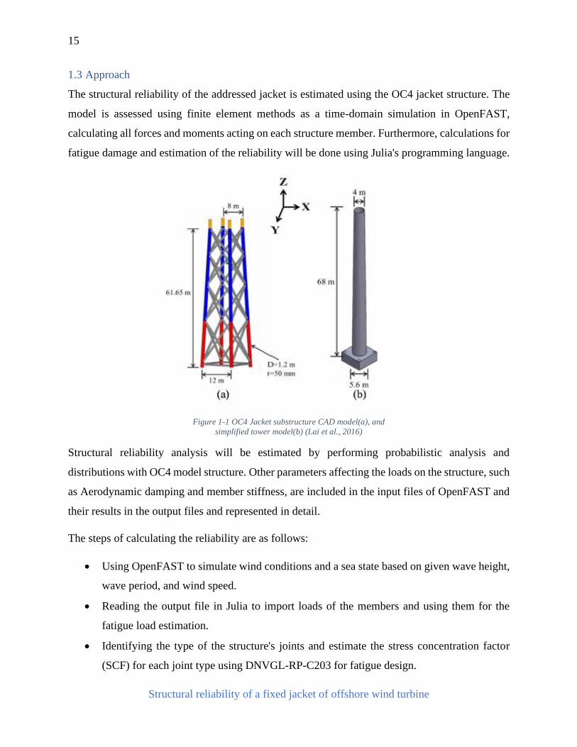
The structural reliability of the addressed jacket is estimated using the OC4 jacket structure. The

model is assessed using finite element methods as a time-domain simulation in OpenFAST,

calculating all forces and moments acting on each structure member. Furthermore, calculations for

fatigue damage and estimation of the reliability will be done using Julia's programming language.

Structural reliability analysis will be estimated by performing probabilistic analysis and

distributions with OC4 model structure. Other parameters affecting the loads on the structure, such

as Aerodynamic damping and member stiffness, are included in the input files of OpenFAST and

their results in the output files and represented in detail.

The steps of calculating the reliability are as follows:

• Using OpenFAST to simulate wind conditions and a sea state based on given wave height,

wave period, and wind speed.

• Reading the output file in Julia to import loads of the members and using them for the

fatigue load estimation.

• Identifying the type of the structure's joints and estimate the stress concentration factor

(SCF) for each joint type using DNVGL-RP-C203 for fatigue design.

Figure 1-1 OC4 Jacket substructure CAD model(a), and

simplified tower model(b) (Lai et al., 2016)

16


• Using the calculated SCFs to estimate the hot spot stresses.

• Using the Rainflow counting method to estimate the fatigue cycles within a time domain.

• Using the outcome from the rainflow counting to obtain the fatigue damage through a

simulation of 60 minutes.

• Using the resulting damage curve along with probability densities of the same wind speeds

using Weibull distribution.

• Implementing different methods to calculate the probability of failure of the structure and

having the numerical solution as the reference value.

• Estimating the reliability from the results obtained from the previous methods.

• Using a meta-model, Gaussian Process, as a new approach to estimate the reliability of the

OC4 jacket.

• Choosing the training data points to be used in the meta-model and developing the best

method of selecting these training observations.

• Comparing the results from the Gaussian Process with the reference value to check the

accuracy of the method.

The damage curve is extracted from a pre-performed analysis of the OC4 model. The model is

assessed in a time-domain simulation. This curve was extracted to implement the deterministic

damage methods (MCI, Bins method, and numerical integration) and obtain the probability of

failure. The Gaussian process is using the Weibull distribution and indicating how the damage

curve should look like, as the curve is unknown.

In this thesis, the last seven points are implemented, starting with using Weibull distribution and

the damage curves and ending with comparing the results obtained from the Gaussian Process with

the other methods. The Gaussian process regression uses the Weibull distribution.

17


1.4 Structure of the thesis

• Chapter 2 presenting a background about wind energy and the calculation of loads caused

by environmental conditions.

• Chapter 3 presents a better understanding of the thesis. It includes the finite elements and

approaches used before and the progress up to date, and how is the probabilistic modelling

is of use along the reliability estimation process.

• Chapter 4 explains the used methodology and detailed approach steps and how the used

approach stands compared to the currently used techniques.

• Chapter 5, the calculations and results of the models and simulations are presented.

• Chapter 6 presents the discussion of the obtained results and how these results are

improving the methods of reliability estimation

• Chapter 7 is presenting the conclusion of the previously shown results and the suggested

further work.

18


Chapter 2: Background

2.1 Offshore wind turbine

Although offshore wind turbines have a high cost, some advantages compensate for this issue. The

higher wind speeds produce magnificently higher power per unit capacity. Offshore wind turbines

also complement solar photovoltaic (PV) as it produces efficiently in winter as the load becomes

at its peak day in and day out throughout the year.

Offshore wind farms began operating in the 1990s. Specifically, the world's first wind farm started

running in 1991 in Vindeby, featuring 0.45 MW turbines. Looking at the wind farms now, they

have more than 14 GW of cumulative installed capacity worldwide[2].

Substructures for offshore wind turbines are humongous, weighing over 1000 tons for wind

turbines of 5 MW.

The substructures of wind turbines are categorized as fixed and floating substructures. In this

thesis, we address the OC4 jacket. OC4 jacket is a fixed substructure that is still in the theoretical

phase, designed but not implemented yet in practice.

2.2 Fixed substructures

The used offshore substructure in this study is the fixed piled structures, primarily used in shallow

water; these structures are widely known as jacket structures. More than 90% of the offshore

platforms existing now are using jacket structure. This type of fixed substructure is a tubular

structure fixed to the seabed by drilled and grouted piles. The water depth for the jacket structure

does not exceed 500m [3], [4].

The types of fixed substructures are:

• Monopile

• Jacket

• Tripod

• Gravity based

Scour can be a problem facing all types of fixed substructures, depending on water depth (WD),

soil type, grading, and seabed current.

19


It might be allowed to develop even longer piles or gravel and rock dump protection required (costs

around €500 -700 k per monopile). Alternatives include frond mats, the so-called plastic seaweed,

rock mats, pile eddy breaking fin or diversion berms, and fences[5].

In offshore structures, failure is caused mainly by insufficient pile strength. The phenomena of

scouring have a significant effect on the load transition and the pile strength[6]. The necessity of

considering scouring phenomena amplifies when the scour depth becomes remarkable, which can

endanger the jacket stability.

The main thing that should be put into consideration is the loads caused by wind and waves. Wave

loads and wind speeds cause many load cases, and the forces acting on the turbine tower can be

calculated using Morison's equation.

Morison's equation calculates the wave force applied to a body by a uniform unsteady flow

𝐷(𝑡) =1

2𝐶𝐷𝐴𝜌𝑈(𝑡)|𝑈(𝑡)| + 𝐶𝑀𝑉𝜌

𝑑𝑈(𝑡)

𝑑𝑡

2-1

Where

V, A: Volume and cross-section area of the body

𝐶𝐷: drag coefficient

𝐶𝑀 = 𝑐𝑚 + 1: inertia force coefficient, where "1" accounts for a hydrostatic force component in

the accelerated fluid.

With assuming having a regular wave, we can use an Airy wave which is a sinusoidal wave.

Airy wave's wave elevation can be determined as:

𝜂(𝑥, 𝑡) =

𝐻

2cos(𝑘𝑥 − 𝜔𝑡) =

𝐻

2𝑅𝑒{𝑒𝑖(𝑘𝑥−𝜔𝑡)}

2-2

And the velocity potential:

𝜙 =

𝑔𝐻2𝜔 cosh

[𝑘(𝑧 + 𝑑)]

cosh(𝑘𝑑)cos(𝑘𝑥 − 𝜔𝑡)

2-3

Dispersion relation:

𝑐2 =𝜔2

𝑘2=𝑔

𝑘tanh(𝑘𝑑)

2-4

20


Where

𝜔2 = 𝑔𝑘 ∗ tanh(𝑘𝑑) 2-5

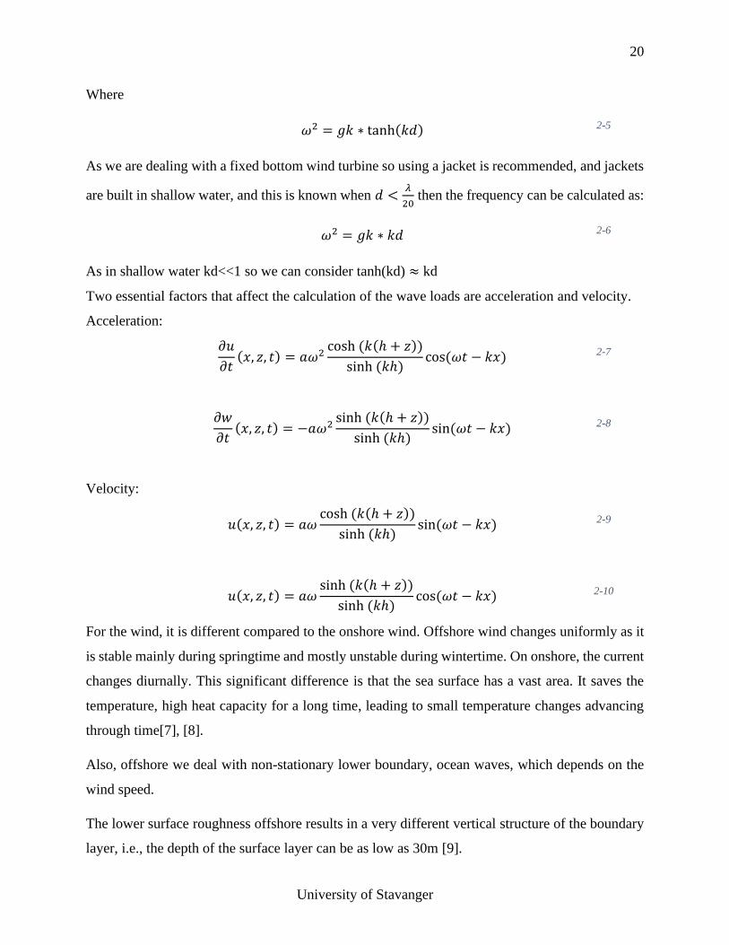
As we are dealing with a fixed bottom wind turbine so using a jacket is recommended, and jackets

are built in shallow water, and this is known when 𝑑 <𝜆

20 then the frequency can be calculated as:

𝜔2 = 𝑔𝑘 ∗ 𝑘𝑑 2-6

As in shallow water kd<<1 so we can consider tanh(kd) ≈ kd

Two essential factors that affect the calculation of the wave loads are acceleration and velocity.

Acceleration:

𝜕𝑢

𝜕𝑡(𝑥, 𝑧, 𝑡) = 𝑎𝜔2

cosh (𝑘(ℎ + 𝑧))

sinh (𝑘ℎ)cos(𝜔𝑡 − 𝑘𝑥) 2-7

𝜕𝑤

𝜕𝑡(𝑥, 𝑧, 𝑡) = −𝑎𝜔2

sinh (𝑘(ℎ + 𝑧))

sinh (𝑘ℎ)sin(𝜔𝑡 − 𝑘𝑥) 2-8

Velocity:

𝑢(𝑥, 𝑧, 𝑡) = 𝑎𝜔cosh (𝑘(ℎ + 𝑧))

sinh (𝑘ℎ)sin(𝜔𝑡 − 𝑘𝑥) 2-9

𝑢(𝑥, 𝑧, 𝑡) = 𝑎𝜔sinh (𝑘(ℎ + 𝑧))

sinh (𝑘ℎ)cos(𝜔𝑡 − 𝑘𝑥) 2-10

For the wind, it is different compared to the onshore wind. Offshore wind changes uniformly as it

is stable mainly during springtime and mostly unstable during wintertime. On onshore, the current

changes diurnally. This significant difference is that the sea surface has a vast area. It saves the

temperature, high heat capacity for a long time, leading to small temperature changes advancing

through time[7], [8].

Also, offshore we deal with non-stationary lower boundary, ocean waves, which depends on the

wind speed.

The lower surface roughness offshore results in a very different vertical structure of the boundary

layer, i.e., the depth of the surface layer can be as low as 30m [9].

21


For the non-stationary boundary layer, we have different wind profile for different wind speeds

The jacket structure is best suitable for shallow water and intermediate water up to 500 m depth.

In shallow water, the waves are long, and as waves move closer to surface water, the phase velocity

decreases. The wave amplitude increases, and the waves start bending, breaking, and making a

significant impact on the structure, causing a substantial load on the jacket's leg and members.

2.3 Power law wind profile

The relation between the wind speeds at a certain height and another is known as the wind profile

power law.

𝑈(𝑧) = 𝑢𝑟𝑒𝑓 (𝑍

𝑍𝑟𝑒𝑓)

𝛼

2-11

Where U is the wind speed at the hub height Z and 𝑢𝑟𝑒𝑓 is the wind speed at the reference hub

height 𝑍𝑟𝑒𝑓 . 𝛼 is the power-law exponent that is a coefficient derived empirically that differs

depending on the atmospheric stability. A commonly used value of 𝛼 is 0.143 in neutral stability

conditions[10], [11].

This method is currently recommended in IEC standards, but this profile does not have a

fundamental physical basis and is only valid for neutral wind conditions.

Figure 2-1 wind profile (Halici and Mutungi, 2016)

22


Figure 2-2 vertical wind shear profile (Maran, Sard 2019)

2.4 Logarithmic wind profile

The log wind profile is a commonly used semi-empirical relationship to define the vertical

distribution within the lowest boundary layer of the horizontal mean wind speed.

The wind speeds logarithmic profile is available within the first 100 m, the so-called surface layer,

of the atmosphere. The rest of the atmospheric layer, up to 1000 m, is composed boundary layer

and the free atmosphere.

𝑈(𝑍) = (𝑢∗𝑘) (ln

𝑍

𝑍0− 𝜑) 2-12

Where 𝑘 = 0.4 refers to Von Karman's constant, z is the height, 𝑢∗ is the friction velocity, z0 is

the surface roughness length, and 𝜑 is a stability-dependent function.

A corrective measure to rely on for the effect of the surface roughness of a wind flow is the

roughness length.

It is challenging to define absolute values because of the indication of the values range by

references.

This method is currently recommended on the DNV standards and is based on Similarity theory.

In most cases, the roughness length 𝑧0 is given based on specific terrain descriptions.

23


Table 2-1 Surface roughness in different terrains

Terrain 𝑘𝑟 𝑍0 𝑍𝑚𝑖𝑛

EN 1991-4

𝑍𝑚𝑖𝑛

Nat. Annex

Sea or coastal area exposed to

the open sea. 0.155 0.003 1 2

Rough open sea, lakes with at

least 5 km fetch upwind and

smooth flat country without

obstacles

0.17 0.01 1 2

Farmland with boundary

hedges, occasional small farm

structures, houses, and trees

0.19 0.05 2 4

Suburban or industrial areas

and permanent forests 0.22 0.3 5 8

Urban areas in which at least

15% of the surface is covered

with buildings and their

average height exceeds 15m

0.24 1 10 16

24


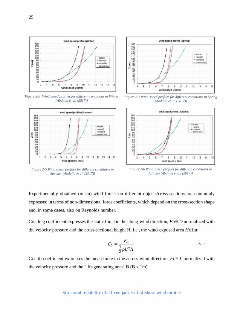
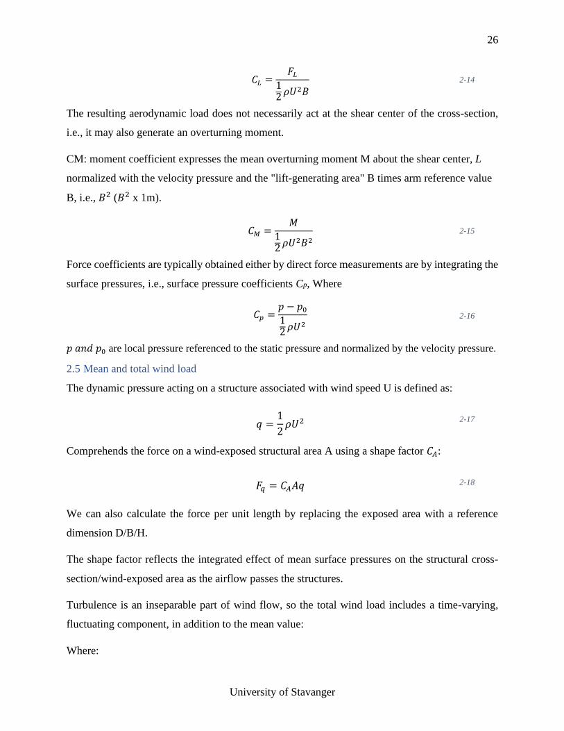
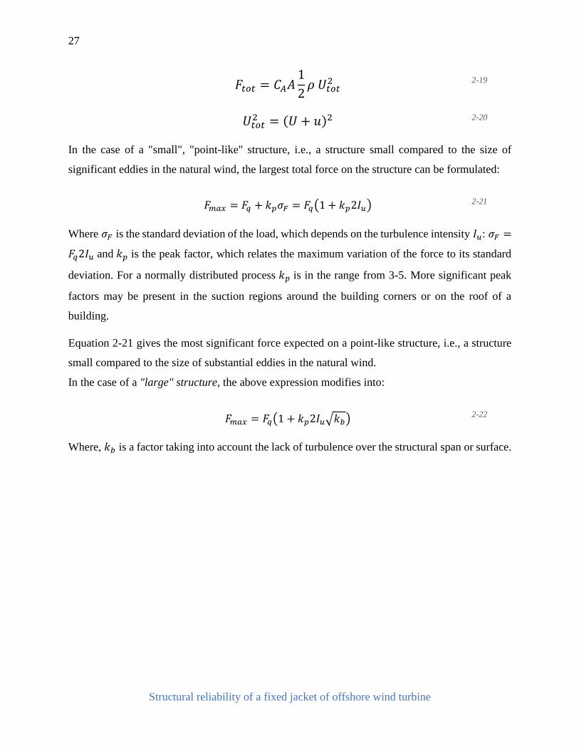
The profiles shown in Figure 2-3 are matched at 30 m, but the roughness length of them all is the

same. The difference in the mean wind gradient is caused by the different instabilities, although

they are for the same terrain and hub height.

Different pressure and temperature gradients with height can cause different stability conditions.

An example of such an effect on the wind profile is shown in Figure 2-4 below [12].

Figure 2-3 wind speed profiles vs static stability in the

surface layer (Abdalla et al., 2017)

Figure 2-4 seasonal cycle of wind shear (Abdalla et al., 2017)

25


Experimentally obtained (mean) wind forces on different objects/cross-sections are commonly

expressed in terms of non-dimensional force coefficients, which depend on the cross-section shape

and, in some cases, also on Reynolds number.

CD: drag coefficient expresses the static force in the along-wind direction, FD ≡ D normalized with

the velocity pressure and the cross-sectional height H, i.e., the wind-exposed area Hx1m:

𝐶𝐷 =𝐹𝐷

12𝜌𝑈

2𝐻 2-13

CL: lift coefficient expresses the mean force in the across-wind direction, FL ≡ L normalized with

the velocity pressure and the "lift-generating area" B (B x 1m).

Figure 2-8 Wind speed profiles for different conditions in Winter

(Abdalla et al. (2017)) Figure 2-7 Wind speed profiles for different conditions in Spring

(Abdalla et al. (2017))

Figure 2-5 Wind speed profiles for different conditions in

Summer (Abdalla et al. (2017)) Figure 2-6 Wind speed profiles for different conditions in

Autumn (Abdalla et al. (2017))

26


𝐶𝐿 =𝐹𝐿

12𝜌𝑈2𝐵

2-14

The resulting aerodynamic load does not necessarily act at the shear center of the cross-section,

i.e., it may also generate an overturning moment.

CM: moment coefficient expresses the mean overturning moment M about the shear center, L

normalized with the velocity pressure and the "lift-generating area" B times arm reference value

B, i.e., 𝐵2 (𝐵2 x 1m).

𝐶𝑀 =𝑀

12𝜌𝑈

2𝐵2 2-15

Force coefficients are typically obtained either by direct force measurements are by integrating the

surface pressures, i.e., surface pressure coefficients Cp, Where

𝐶𝑝 =

𝑝 − 𝑝012𝜌𝑈

2 2-16

𝑝 𝑎𝑛𝑑 𝑝0 are local pressure referenced to the static pressure and normalized by the velocity pressure.

2.5 Mean and total wind load

The dynamic pressure acting on a structure associated with wind speed U is defined as:

𝑞 =1

2𝜌𝑈2

2-17

Comprehends the force on a wind-exposed structural area A using a shape factor 𝐶𝐴:

𝐹𝑞 = 𝐶𝐴𝐴𝑞 2-18

We can also calculate the force per unit length by replacing the exposed area with a reference

dimension D/B/H.

The shape factor reflects the integrated effect of mean surface pressures on the structural cross-

section/wind-exposed area as the airflow passes the structures.

Turbulence is an inseparable part of wind flow, so the total wind load includes a time-varying,

fluctuating component, in addition to the mean value:

Where:

27


𝐹𝑡𝑜𝑡 = 𝐶𝐴𝐴1

2𝜌 𝑈𝑡𝑜𝑡

2 2-19

𝑈𝑡𝑜𝑡2 = (𝑈 + 𝑢)2

2-20

In the case of a "small", "point-like" structure, i.e., a structure small compared to the size of

significant eddies in the natural wind, the largest total force on the structure can be formulated:

𝐹𝑚𝑎𝑥 = 𝐹𝑞 + 𝑘𝑝𝜎𝐹 = 𝐹𝑞(1 + 𝑘𝑝2𝐼𝑢) 2-21

Where 𝜎𝐹 is the standard deviation of the load, which depends on the turbulence intensity 𝐼𝑢: 𝜎𝐹 =

𝐹𝑞2𝐼𝑢 and 𝑘𝑝 is the peak factor, which relates the maximum variation of the force to its standard

deviation. For a normally distributed process 𝑘𝑝 is in the range from 3-5. More significant peak

factors may be present in the suction regions around the building corners or on the roof of a

building.

Equation 2-21 gives the most significant force expected on a point-like structure, i.e., a structure

small compared to the size of substantial eddies in the natural wind.

In the case of a "large" structure, the above expression modifies into:

𝐹𝑚𝑎𝑥 = 𝐹𝑞(1 + 𝑘𝑝2𝐼𝑢√𝑘𝑏) 2-22

Where, 𝑘𝑏 is a factor taking into account the lack of turbulence over the structural span or surface.

28


2.6 Mal functions of components

The downtimes calculated are due to both regular maintenance and unexpected malfunctions. The

following evaluations refer only to the unexpected malfunctions, which concerned half mechanical

and half electrical components[13].

Regardless of failure rates, downtimes of machines after a failure are an essential factor in defining

a machine's reliability. Downtime duration caused by malfunctions is dependent on necessary

maintenance and repair work, replacement parts availability, and the personnel capacity of service

teams. Previously, generator repairs, drive train, hub, gearbox, and blades have usually caused

hold periods of several weeks [14].

Figure 2-9 main components' share of the total number of failures

(Hossain et al., 2018)

29


Considering all the reported repair measures that are available now, the average rate of failure and

downtime per component can be given. It is noticed that the downtimes declined in the past five

to ten years. So, the high number of failures of some components is now balanced out to a certain

extent by short standstill periods. However, damages to generators, gearboxes, and drive trains are

mainly caused by extended downtime of one week as an average [15], [16].

The industry-accepted turbine lifetime is 20 years. Thus, a wind turbine's reliability is the

percentage of time that the turbine will be functioning at total capacity during appropriate wind

conditions at a site with specified wind resource characterization for a 20-year life. Reliability

specialists use a graphical representation called the bathtub curve. The bathtub curve consists of

three regions; an infant mortality period with a decreasing failure rate followed by an average life

period with a low and relatively constant failure rate and ending with displaying an increasing

failure rate of the wear-out period[17], [18].

2.7 Fatigue Analysis

The primary failure focused on in this thesis is fatigue failure. Fatigue is the most common type

of failure an offshore structure experiences due to the different and cyclic environmental loads

applied by the wind and waves. Defining the type of joints is required to understand the fatigue

Figure 2-10 Reliability characteristics for different components of wind turbine (Faulstich et al., 2011)

30


subjected to the OC4 jacket, as there are different types of joints such as T, X, Y, K, and complex

joints.

In the DNV-RP-C203 standard for fatigue design, different types of fatigue modes and joints types

are mentioned. As the jacket addressed is made of tubular joints, the nominal stress can be

calculated using the simple beam theory as:

𝜎𝑁𝑜𝑚𝑖𝑛𝑎𝑙 =

𝑃

𝐴±𝑀

𝐼𝑦

2-23

Where P is the applied axial load, A is the cross-sectional area, M is the applied bending moment,

I is the inertia of the section area about the neutral axis, and y is the perpendicular distance from

the neutral axis to a point on the section. [19]

The intriguing matter is what defines the axial load. The most probable guess is that the x-axis is

where the axial load exists, to make sure this is the right guess, the local axis has to be transformed

into the correct coordinate to define the direction of every load in x y and z. This transformation

can be done by multiplying the transpose of the transformation matrix by the load vector[20]. After

estimating the nominal stresses, we need to calculate the fatigue damage, which is defined in DNV

standard as it is dependent on the S-N curve and is estimated as:

𝐷 = ∑

𝑛𝑖𝑁𝑖

𝑘

𝑖=1

=1

�̅�∑𝑛𝑖 . (∆𝜎𝑖)

𝑚

𝑘

𝑖=1

2-24

Where

D = accumulated fatigue damage

�̅� = intercept of the design S-N curve with the log N axis

m = negative inverse slope of the S-N curve

k = number of stress blocks

ni = number of stress cycles in stress block i

Ni = number of cycles to failure at constant stress range Δσi

31


As shown in the equation, stress is the hot spot stress, and the hot spot stress is the stress that we

are most interested in. The hot spot stress is simply calculated by multiplying the nominal stress

by a stress concentration factor (SCF). Defining the type of the joints depend on the direction of

the forces and moments, if the load is compression or tension, and if the moment is in-plane or out

of plane. Having the global to local transformation matrices from the output files, the definition of

the in-plane and out of plane became more accessible as we can assume a coordinate system of

local x, y, and z and then use the inverse of the global to local transfer matrices and then

transforming from the global back to the assumed coordinate system.

Figure 2-11 classification of joints (DNVGL-RP-C203)

32


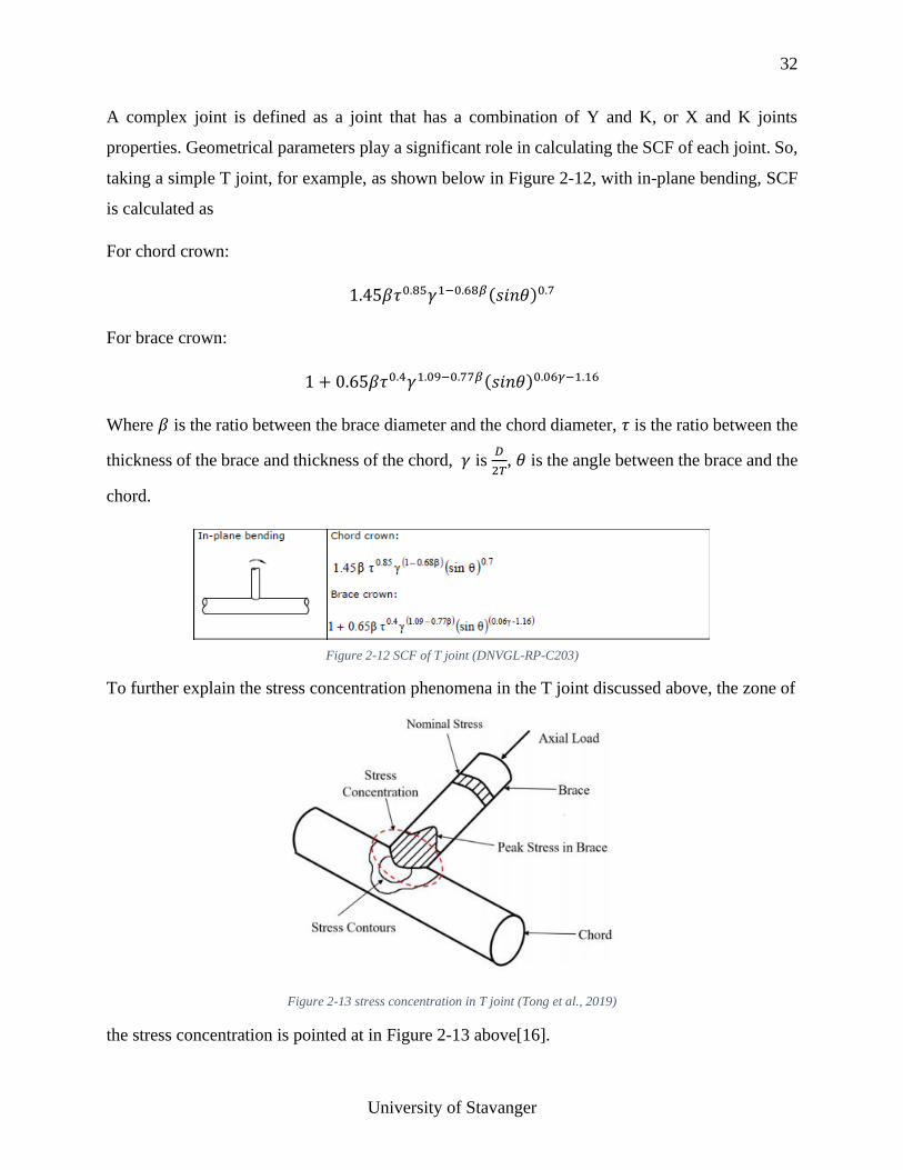
A complex joint is defined as a joint that has a combination of Y and K, or X and K joints

properties. Geometrical parameters play a significant role in calculating the SCF of each joint. So,

taking a simple T joint, for example, as shown below in Figure 2-12, with in-plane bending, SCF

is calculated as

For chord crown:

1.45𝛽𝜏0.85𝛾1−0.68𝛽(𝑠𝑖𝑛𝜃)0.7

For brace crown:

1 + 0.65𝛽𝜏0.4𝛾1.09−0.77𝛽(𝑠𝑖𝑛𝜃)0.06𝛾−1.16

Where 𝛽 is the ratio between the brace diameter and the chord diameter, 𝜏 is the ratio between the

thickness of the brace and thickness of the chord, 𝛾 is 𝐷

2𝑇, 𝜃 is the angle between the brace and the

chord.

To further explain the stress concentration phenomena in the T joint discussed above, the zone of

the stress concentration is pointed at in Figure 2-13 above[16].

Figure 2-13 stress concentration in T joint (Tong et al., 2019)

Figure 2-12 SCF of T joint (DNVGL-RP-C203)

33


As shown in Figure 2-13, it is clear that the stress at the welded joint is higher than the nominal

stress due to the stress concentration.

The main goal is to calculate the damage done to the joint due to environmental conditions.

Calculating the nominal stress is the main procedure for calculating the damage.

However, the stress we are interested in is the hot spot stress, and that is calculated by multiplying

the SCF by the nominal stress calculated.

To analyze the design, a simplified numerical procedure is implemented to reduce the demand for

large fine-mesh models for the calculation of SCF factors:

• the stress concentration or the notch factor due to the weld itself is included in the S-N

curve to be used, the D-curve. This S-N curve is also known as the hot spot S-N curve.

Figure 2-14 Definition of geometrical parameters (DNVGL-RP-C203)

34


• The stress concentration due to the geometric effect of the precise detail can be calculated

using different methods, such as considering the use of solid elements, resulting in a

geometric SCF factor.

This procedure is defined as the hot spot method.

The hot-spot stress method, which is also known as the geometric stress method, considers the

stress increment effect due to the structural discontinuity except for the stress concentration due to

weld toe, i.e., without the consideration of the localized weld notch stress. Hot spot stress is the

value of the structural stress of the surface at hot spots. The hot spots are located at a welded joint

where the cracks possibly initiate under cyclic loading due to the increased stress value.

In the hot spot stress method, the fatigue life is related to hot spot stress directly instead of the

nominal stress. The fatigue life of tubular and non-tubular joints is usually identified using S−N

curves. An S −N curve shows the relation between the hot spot stress range and the number of

cycles to failure. The performance fatigue life of tubular and non-tubular joints is also dependent

on the structural members' thickness. The fatigue life of tubular and non-tubular joints gets

decreased as the thickness of the structural member increases.

35


Chapter 3: Literature Review

The offshore wind industry faces many challenges in the support structures design process, and

the main challenge would be the cost of design. The main goal of reliability analysis is to have an

optimal design with a lower cost. When we address fatigue damage assessment, we often discuss

the fatigue load of an offshore wind turbine in time-domain simulations, which leads to a long

process. To obtain a high level of accuracy in the results, we use a large number of load cases, and

the objective to be achieved here is reaching an accurate solution with a lower number of load

cases. There are many approaches applied to achieve this goal using statistical models.

3.1 Modelling of uncertainties in structural engineering

Close to all input parameters in a structural design problem is associated with uncertainties, which

need to be addressed in the analysis. As an example, the load on a turbine has uncertainties due to

the randomness of the environmental conditions, such as the wind speed. Furthermore, it is

associated with uncertainty in, for example, the drag coefficient (𝐶𝑑 ). In addition, there are

uncertainties in system parameters, such as the damping coefficient and the stiffness of the soil.

The modelling of these uncertainties is a crucial point within the formulation of a structural

problem of offshore wind turbines. There are several mathematical and statistical models to

describe these uncertainties in a probabilistic model of the structure.

A probability distribution is a statistical function. The function describes the likelihoods that a

random variable can obtain in a range of given numbers. The probability distribution functions are

typically described by their mean, standard deviation, kurtosis, and skewness.

The normal distribution is the most common. The normal distribution is frequently used in

Engineering, investing, finance, and science. The normal distribution is defined and characterized

by its mean and standard deviation, which means that the distribution is neither skewed nor exhibits

kurtosis, which makes the distribution symmetric.

To the probability of occurrence of uncertain events which are naturally stochastic, two main

functions are used, and those are the probability density function and cumulative density function.

To describe a random variable statistically, it can be entirely described by using a cumulative

density function as 𝐹𝑋(𝑥) or by using a probability density function 𝑓𝑋(𝑥), shown as follows

36


𝐹𝑋(𝑥) = 𝑃(𝑋 ≤ 𝑥) = ∫ 𝑓𝑋(𝑥)𝑑𝑥𝑥

−∞

3-1

The distribution of the variables is defined by some parameters in association with the probability

distribution. These parameters are known as statistical moments. Known that the most commonly

used moments are the mean value 𝜇(𝑋), known as the first moment, and also called the expected

value as denoted by E(X), and the second moment, known as variance and denoted by 𝜎2(𝑋) or

Var(X). the two moments (parameters) can be described as follows:

𝑀𝑒𝑎𝑛: 𝜇(𝑋) =∑ 𝑋𝑖𝑁𝑖=1

𝑁

3-2

𝑣𝑎𝑟𝑖𝑎𝑛𝑐𝑒: 𝜎2(𝑋) =∑(𝑥 − 𝜇)2

𝑁

3-3

The probability distributions used for structural engineering are log-normal, uniform, and Weibull

distributions. A significant parameter in the distributions is the coefficient of variation (CV), and

it is defined as the standard deviation divided by the mean value[21].

𝐶𝑉 =𝜎

𝜇 3-4

37


A very common continuous distribution presenting the probability is the normal or Gaussian

distribution. One can define the density function of such probability distribution by plotting a curve

with specific mean and standard deviation as follows:

𝑓(𝑥; 𝜇, 𝜎) =1

𝜎√2𝜋𝑒−(𝑥−𝜇)2

2𝜎2 =1

𝜎𝜑 ((𝑥 − 𝜇)

𝜎) 3-5

Where

𝜑(𝑥) =1

√2𝜋𝑒−

12𝑥2

3-6

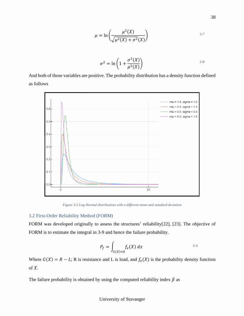
Another type of continuous probability distribution is the log-normal distribution. The log-normal

distribution has random variables that possess a logarithm that is normally distributed.

To plot a distribution with specific mean 𝜇(𝑥) and variance 𝜎2(𝑥) we can use

Figure 3-1 density functions with different mean and standard deviation

38


𝜇 = ln(𝜇2(𝑋)

√𝜇2(𝑋) + 𝜎2(𝑋)) 3-7

𝜎2 = ln (1 +𝜎2(𝑋)

𝜇2(𝑋)) 3-8

And both of those variables are positive. The probability distribution has a density function defined

as follows

Figure 3-2 Log-Normal distributions with a different mean and standard deviation

3.2 First-Order Reliability Method (FORM)

FORM was developed originally to assess the structures’ reliability[22], [23]. The objective of

FORM is to estimate the integral in 3-9 and hence the failure probability.

𝑃𝑓 = ∫ 𝑓𝑥(𝑋) 𝑑𝑥

𝐺(𝑋)<0

3-9

Where 𝐺(𝑋) = 𝑅 − 𝐿; R is resistance and L is load, and 𝑓𝑥(𝑋) is the probability density function

of 𝑋.

The failure probability is obtained by using the computed reliability index 𝛽 as

39


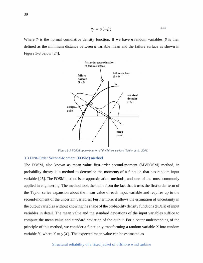
𝑃𝑓 = 𝛷(−𝛽) 3-10

Where 𝛷 is the normal cumulative density function. If we have 𝑛 random variables, 𝛽 is then

defined as the minimum distance between 𝑛 variable mean and the failure surface as shown in

Figure 3-3 below [24].

3.3 First-Order Second-Moment (FOSM) method

The FOSM, also known as mean value first-order second-moment (MVFOSM) method, in

probability theory is a method to determine the moments of a function that has random input

variables[25]. The FOSM method is an approximation methods, and one of the most commonly

applied in engineering. The method took the name from the fact that it uses the first-order term of

the Taylor series expansion about the mean value of each input variable and requires up to the

second-moment of the uncertain variables. Furthermore, it allows the estimation of uncertainty in

the output variables without knowing the shape of the probability density functions (PDFs) of input

variables in detail. The mean value and the standard deviations of the input variables suffice to

compute the mean value and standard deviation of the output. For a better understanding of the

principle of this method, we consider a function y transforming a random variable X into random

variable Y, where 𝑌 = 𝑦(𝑋). The expected mean value can be estimated as

Figure 3-3 FORM approximation of the failure surface (Maier et al., 2001)

40


𝐸(𝑌) = ∫ 𝑦(𝑥)𝑝𝑋(𝑥)𝑑𝑥∞

−∞

3-11

And the variance is

𝑉𝑎𝑟(𝑌) = ∫ [𝑦(𝑥) − 𝐸(𝑌)]2𝑝𝑋(𝑥)𝑑𝑥∞

−∞

3-12

Where 𝑝𝑋 is the PDF of 𝑋. The mean and variance of 𝑌 require information of 𝑝𝑋, which in many

cases the available information is limited to the mean and variance of 𝑋 . Furthermore, even

knowing 𝑝𝑋, the computation of the integrals in Equations 3-11and 3-12 may, to a great extent,

consume time (Ang & Tang, 1975) [26].

3.4 Structural Reliability Analysis

The goal is to determine how reliable these structures are, using a statistical model that reduces

uncertainties in the estimates of the probability of failure of the jacket.

Structural reliability is capable of including uncertainties in the parameters of a structural system

and the different environmental loads.

A deterministic approach to structural engineering is typically based on the partial factor, and limit

state method, also called the Load and Resistance Factor Design (LRFD). This method addresses

uncertainties in parameters by determining the characteristic values of material properties and load

intensities. In addition, partial safety factors are used to cope with some aspects of uncertainty.

However, it might not in all cases be cost-optimal and may in some cases be too much on the safe

side. Hence, for offshore wind turbines, it is of interest to investigate methods such as structural

reliability analysis in order to seek a more cost-efficient design.

A suitable way of obtaining this, probability of failure, the risk is the approach of probabilistic

models. Such an approach allows designing the structure with a sufficient and acceptable

probability of failure during the structure's lifetime.

The simplest problem of structural reliability is illustrating this theory. If we consider a single load

effect S that is resisted by a single resistance R. each of these parameters is defined by a known

probability density function, 𝑓𝑆 and 𝑓𝑅 respectively, expressing both R and S in the same unit, as

illustrated in Figure 3-4.

41


Figure 3-4 reliability-based design curve (Melchers, 2018)

The failure of the structure in this simple example can be considered to occur if the resultant S is

surpassing the resistance R. The probability of failure of an element can be defined as follows [27],

[28].

𝑝𝑓 = 𝑃(𝑔(𝑅, 𝑆) ≤ 0) 3-13

Where 𝑔 is the limit state, and the failure probability is the same as the probability of violating the

limit state. Equation 3-13 can be used to estimate the probability failure of a probabilistic model

for the number of observations considered in the analysis. A reliability analysis is required for the

statistical description of the limit state values 𝑔𝑖(𝑖 = 1,2,3, … , 𝑛) . Defining the statistical

characteristics using the most suitable probability distributions is an essential step before

implementing reliability analysis. Eventually, the probability of failure is estimated using

numerical calculations efficiently and economically.

This is known as “convolution integral”, with meaning easily explained as shown in Figure 3-5.

Figure 3-5 Basic R-S problem (Melchers, R.E., 2018)

42


𝐹𝑅(𝑥) is the probability that 𝑅 ≤ 𝑥 or the probability that actual resistance R of the member is less

than range value x. This failure is represented if the loading is larger than 𝑥. The probability of this

case is given by the term 𝑓𝑆(𝑥) that represents the probability of the load effect S that acts in the

member has a value between 𝑥 and 𝑥 + ∆𝑥 in the limit as ∆𝑥 goes towards zero. By considering

all possible values of x, i.e. by taking the integral over all x, the total failure probability is obtained.

𝑃𝑓 = ∫ (1 − 𝐹𝑠(𝑥))𝑓𝑅(𝑥)𝑑𝑥∞

−∞

3-14

This can be defined as the summation of the failure probabilities of the load that exceeds the

resistance.

Numerous methods have been developed aiming to obtain the integrated probability in structural

reliability analysis. The most common methods are the first and second-order reliability methods

(FORM and SORM) and Monte Carlo simulation. Direct methods to integrate over the failure

domain is also in use by different numerical integrating methods, such as the Newton-Raphson

method, Monte Carlo Integration and the so-called Bins method. These approaches aimed to

estimate the failure probability from the data provided by the test of many samples and data

points[29], [30].

The term Structural reliability of a structure refers to the probability of safe performance of a limit

state. Limit states refer to ultimate failures, such as collapse, or unserviceability, such as deflection,

vibrations, or crack propagation. An efficient way to designing a structure is using a probabilistic

model to treat structural loads and resistance. Structural reliability is becoming the ideal way of

designing a structure as it replaces the deterministic traditional ways of maintenance and design.

The reliability can be estimated as

𝑅𝑒𝑙𝑖𝑎𝑏𝑖𝑙𝑖𝑡𝑦 = 1 − 𝑃𝑓𝑎𝑖𝑙𝑢𝑟𝑒

The reliability-based design has the objective of ensuring that the failure probability of a system

is reasonably low.

3.5 Bins Method

The bins method, or as known Numerical Binning, is a method to group or collect a number of

more or fewer values which are continuous into smaller bins number. Creating bins or ranges helps

43


in understanding the numerical data in a better way. Taking, an example, data on the age of a group

of people, we might want to have their ages arranged into a smaller number of age intervals.

The same thing can be illustrated in the data collected to calculate the reliability of a structure from

having the damage of every wind speed ranging from 0 to 40𝑚/𝑠. Arranging this wind speed range

into smaller groups, 5𝑚/𝑠 for example, helps in understanding the data sets better than taking the

whole range at once[31].

3.6 Monte Carlo Integration

The numerical integration in mathematics uses equally spaced numbers in calculations. The

difference between Monte Carlo Integration and numerical integration is the use of random

numbers.

A simple way to illustrate this method is integrating a univariant function s denoting by S the

integral value

𝑆 = ∫ 𝑠(𝑥)𝑑𝑥𝑏

𝑎

This integral can be considered as the area below the curve of the function. Taking a random

function as

𝑠(𝑥) = 𝑥2 − 3𝑥 + 2

The function can be plotted as shown in Figure 3-6 above and choosing 𝑎 = −2 and 𝑏 = 5

Figure 3-6 𝑥2 − 3𝑥 + 2

44


If we choose a random 𝑥 value between 𝑎 and 𝑏, multiplying 𝑠(𝑥) by (𝑏 − 𝑎), we get the area of

a rectangle width of 𝑏 − 𝑎 and the height of 𝑥. The main reason why Monte Carlo is to estimate

an approximation of the integral value by the average area of the rectangles shown in Figure 3-7

below, computed for random chosen 𝑥 values [32].

By summing the area of the rectangles and obtaining the average of the sum, the number keeps

getting closer to the actual result of the integral. The idea is generally formalized as

𝐹𝑁 = (𝑏 − 𝑎)1

𝑁 − 1∑𝑓(𝑋𝑖)

𝑁

𝑖=0

Where 𝑋𝑖 is the random variable chosen for every rectangle. Large numbers have a law that gives

us that as N tends to infinity, the true value of the integral becomes:

𝑃𝑟( lim𝑁→∞

(𝐹𝑁) = 𝐹) = 1

That means that the more numbers are used in this method, the more accurate the results become.

The Monte Carlo method has been used before for reliability estimation with some limitations of

simplifying the structure. This method showed relatively well performance, managing to assess

Figure 3-7 summing the rectangles (Cumer et al. 2020)

45


structural reliability with doable effort. The results obtained by this approach is indicating the

importance of the probabilistic assessment in the optimization of a structure’s design [33].

3.7 Numerical Integration

The numerical integration method is computing an approximation to the integral of a certain

function. In structural reliability, numerical integration can be used for obtaining the failure

probability in a high accuracy manner. The use of this method starts with combining the

probabilities with the required parameter to be assessed and integrate them numerically.

Numerical integration is still used to estimate structural reliability, and it showed higher accuracy

than the traditional first-order second-moment method (FOSM). When a small number of points

is used, it shows lower accuracy yet satisfying to the accuracy requirement in engineering. With a

higher number of points, the accuracy increases accordingly[34], [35].

3.8 Gaussian Process

The Gaussian Process is a stochastic process with random variables defined by time and space,

and every collection of those variables has a multivariate normal distribution. The process allows

predicting the available data by incorporating previous knowledge. It is commonly used in fitting

a function of the data, which is basically called regression.

The Gaussian process as a tool is powerful in machine learning. It is not limited to regression but

can also be used in classification tasks. Each data set has infinitely many functions to help with

fitting the data. The Gaussian process gives a creative and elegant solution to this problem by

simply assigning probabilities to every function. Additionally, the use of probabilistic approaches

allows us to include the confidence of the regression results from the prediction[36].

The model can then predict the mean and variance of function value at new points. The main

Gaussian process is defined as

𝑓(𝑥)~𝐺𝑃(𝑚(𝑥), 𝑘(𝑥, 𝑥′))

Where 𝑚(𝑥) is the mean function and 𝑘(𝑥, 𝑥′) is the kernel function. The mean function gives the

mean at any point of the input space, and the kernel sets the covariance between points. Usually,

the mean is set to zero for simplicity, and the kernel should be positive definite[37].

46


A Gaussian process regression (GPR) defines a probabilistic model over a set of given data points.

It is constructed so that the probability of the value of the function is maximized for all given data

points. The process is successfully used in many fields such as Internet of Things (IoT), prediction

analysis of time series, and dynamic system control[38]–[40]. GPR method, however, continues

to possess a few deficiencies such as calculations and limitation of the noise distribution. Studies

revealed that selecting the hyperparameters significantly affect the GPR performance. The optimal

selection of these hyperparameters leads to significant reduction of iterations of GPR learning and

improve the accuracy of model fitting. Optimizing the parameters can be done using experiment

trials and experience selection. However, these types of optimizing methods involve deficiencies,

including the high cost of calculation and poor efficiency[41]. In this thesis, the GPR is

implemented in Julia, where two optimization methods: conjugate gradient and L-BFGS.

Conjugate gradient (CG) is a solver which is iterative, used for linear equation systems 𝐴𝑥 = 𝑏

where 𝐴 ∈ ℝ𝑁∗𝑁 a real, positive definite, and symmetric matrix. In practice, CG is used as an

approximate solver, and it can provide a good estimation to 𝑥 in significantly small 𝑁 steps[42].

The Broyden-Fletcher-Goldfarb-Shanno (BFGS) is an iterative method for solving unconstrained

nonlinear optimization problems. Furthermore, L-BFGS is using a limited amount of computer

memory. It is a typical algorithm for parameter estimation in machine learning. This algorithm’s

target problem is to minimize 𝑓(𝑥) over unconstrained values of the real vector 𝑥 where 𝑓 is a

differential scalar function.

The use of the Gaussian process in structural reliability in previous studies showed promising

results with the process managing to significantly reduce the number of required training data

points and providing accurate estimations of the failure probability when compared to the

FORM[43], [44].

47


Chapter 4: Methodology

The methodology of this thesis objectives is the approach of using statistical modelling to obtain

the fatigue reliability of the jacket structure. The industry uses methods that are time-consuming

and costly, implementing the different numerical approaches with deterministic damage values to

compare between them and the applied approach, statistical model, of the Gaussian Process. The

comparison will show how the statistical approach is standing against the currently used methods

in terms of accuracy and time efficiency.

The Gaussian process is defined by its mean and covariance functions, where the mean function

𝑚(𝑥) describes the mean of any point in the process, and the kernel 𝑘(𝑥, 𝑥′) = 𝜎2 describes the

covariance between two training points.

The Gaussian process is a non-parametric model. That makes it easier as we do not have to worry

about fitting too much data, training, points added to the model, unlike a linear model on a non-

linear data point.

4.1 Wind Distribution

The wind speed probability is in the thesis modelled by a Weibull distribution.

Figure 4-1 Weibull distribution

48


4.2 Damage Curve

The damage curve used in this thesis is extracted from the results obtained from the research article

“Simplified fatigue load assessment in offshore wind turbine structural analysis” written by Daniel

Zwick and Michael Muskulus [45]. For each member connected to a Y-joint, K-joint or X-joint,

FEDEM Windpower was used to establish the time series data for the axial force as well as in-

plane and out-of-plane bending moments as outputs. From the raw time series data, a transient of

60 to 200 seconds was cut off depending on the wind speed. The simulation produced results in a

total analysis length of 60 minutes. Force and moment time series were converted to sectional

stresses, using beam cross-section data for the specific members. Using Equation 2-24, these time

series are adjusted by the relevant SCF, and then a rainflow counting method is used in order to

get the 𝑛 and ∆𝜎. With these and the relevant 𝑆 − 𝑁 curve, the total damage is calculated.

Figure 4-2 Damage curve

4.3 Total damage estimation

The results of the damage and the probability density function corresponding to wind speed are

obtained for the jacket.

The total damage required to estimate the reliability is obtained using four methods:

• Damage estimation using numerical integration

• Damage estimation using bins method

49


• Damage estimation using Monte Carlo Integration (MCI)

• Damage estimation using Gaussian Process

4.3.1 Numerical Integration

This method demands combining the damage curve with the probability density distribution and

then integrating them numerically at every damage position for every wind speed. The results

obtained from numerical integration are considered, in this thesis, as the reference results.

4.3.2 Bins Method

This method is implemented by obtaining the probabilities by integrating the probability densities

at every wind speed and then multiplying these probabilities with every damage corresponding to

the same wind speeds.

4.3.3 Monte Carlo Integration

In numerical integration, the used methods are using a deterministic approach in obtaining the total

damage. However, Monte Carlo integration utilizes a non-deterministic approach. Each set of

chosen points give a different outcome as they are chosen randomly. The outcome is an

approximation of the true value or the reference value of the total damage, which is the numerical

integration, value with respective error bars. These error bars are likely to contain the reference

value or the required accurate value.

This method is implemented with the same procedure as the Bins method in having the

probabilities estimated and then combining each probability with the corresponding damage.

4.3.4 Failure probability using deterministic value

The total damage estimated using the three previously explained methods is used to obtain the

failure probability by integrating the PDF of the normal distribution of 𝜇 = 1 𝑎𝑛𝑑 𝜎 = 0.3 with

the total damage. This integral can be descriped as shown in Figure 5-2 in Chapter 5:.

50


4.3.5 Gaussian Process

The Gaussian Process still possesses high uncertainty in controlling the distribution using its length

scale and standard deviation. In Julia, the used package "GaussianProcess" requires four inputs:

training data in X and Y, the kernel, and the gaussian mean. The Gaussian process is mainly

controlled by its mean and kernel. The kernel is dependent on two variables: the length scale and

standard deviation. The used type of kernel in this thesis is the squared exponential kernel, and it

can be described as shown in Figure 4-3 below

Controlling the kernel is implemented by fixing a mean with a zero value and changing the kernel

accordingly by choosing the data points.

After plotting the gaussian distribution, the mean curve values and the variance are obtained using

a prediction function in the "GaussianProcess" package. Then the mean and the covariance matrix

are calculated using those predicted data generated.

Figure 4-3 gaussian and exponential kernel plot (Rasmussen and Williams, 2006)

51


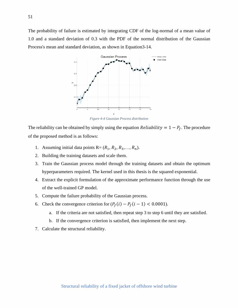
The probability of failure is estimated by integrating CDF of the log-normal of a mean value of

1.0 and a standard deviation of 0.3 with the PDF of the normal distribution of the Gaussian

Process's mean and standard deviation, as shown in Equation3-14.

The reliability can be obtained by simply using the equation 𝑅𝑒𝑙𝑖𝑎𝑏𝑖𝑙𝑖𝑡𝑦 = 1 − 𝑃𝑓. The procedure

of the proposed method is as follows:

1. Assuming initial data points R= (𝑅1, 𝑅2, 𝑅3,…, 𝑅𝑛).

2. Building the training datasets and scale them.

3. Train the Gaussian process model through the training datasets and obtain the optimum

hyperparameters required. The kernel used in this thesis is the squared exponential.

4. Extract the explicit formulation of the approximate performance function through the use

of the well-trained GP model.

5. Compute the failure probability of the Gaussian process.

6. Check the convergence criterion for (𝑃𝑓(𝑖) − 𝑃𝑓(𝑖 − 1) < 0.0001).

a. If the criteria are not satisfied, then repeat step 3 to step 6 until they are satisfied.

b. If the convergence criterion is satisfied, then implement the next step.

7. Calculate the structural reliability.

Figure 4-4 Gaussian Process distribution

52


Chapter 5: Results

5.1 Damage Estimation

The total damage is estimated using both the probability densities from the Weibull distribution

and the damage distribution.

5.1.1 Damage Estimation Using Bins Method

As explained before in the Bins method, the process requires estimating the probabilities by

integrating the probability densities with the wind speeds.

• Using N = 7, we get a damage of 0.2558089937513546



As shown from the results above, the more bins we use, the more accurate the results are. Reaching

a high number of samples shows results very close to the reference value with a difference of

almost 0.0001%.

5.1.2 Damage Estimation Using Monte Carlo Integration

The difference between Monte Carlo Integration and the Bins method is that Monte Carlo chooses

random points to evaluate the damage. In contrast, the Bins method chooses specific points to

evaluate the damage.

• Using an "Rn" value of 100, we get a damage value of 0.25726065445676505



As we can observe from the above-shown results, the more points we used, the closer we get to

the reference value of the numerical integration. Using 1000000 showing a difference of almost

0.0004% between Monte Carlo damage and the reference damage.

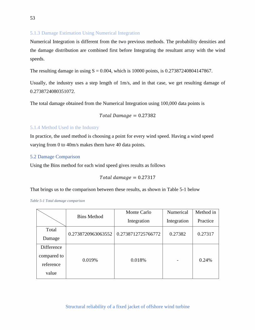
53


5.1.3 Damage Estimation Using Numerical Integration

Numerical Integration is different from the two previous methods. The probability densities and

the damage distribution are combined first before Integrating the resultant array with the wind

speeds.

The resulting damage in using S = 0.004, which is 10000 points, is 0.27387240804147867.

Usually, the industry uses a step length of 1m/s, and in that case, we get resulting damage of

0.2738724080351072.

The total damage obtained from the Numerical Integration using 100,000 data points is

𝑇𝑜𝑡𝑎𝑙 𝐷𝑎𝑚𝑎𝑔𝑒 = 0.27382

5.1.4 Method Used in the Industry

In practice, the used method is choosing a point for every wind speed. Having a wind speed

varying from 0 to 40m/s makes them have 40 data points.

5.2 Damage Comparison

Using the Bins method for each wind speed gives results as follows

𝑇𝑜𝑡𝑎𝑙 𝑑𝑎𝑚𝑎𝑔𝑒 = 0.27317

That brings us to the comparison between these results, as shown in Table 5-1 below

Table 5-1 Total damage comparison

Bins Method Monte Carlo

Integration

Numerical

Integration

Method in

Practice

Total

Damage 0.2738720963063552 0.2738712725766772 0.27382 0.27317

Difference

compared to

reference

value

0.019% 0.018% - 0.24%

54


5.3 Reliability estimation

Estimating the reliability using the load resistance method in deterministic values is done by

integrating the lognormal curve with the damage resulting from the methods above. The normal

distribution, in this case, has a mean of 1 and a CV of 0.3. the lognormal parameters can be

calculated as follows:

Mean = exp (𝜇 +𝜎2

2) = 1

Variance = [exp(𝜎2) − 1] exp(2𝜇 + 𝜎2) = 0.3

So, 𝜇 = −0.0431 and 𝜎 = 0.2935

The lognormal is then integrated with the deterministic damage estimated above.

Figure 5-1 lognormal distribution

Figure 5-2 integrating lognormal with deterministic damage

55


The integration result is simply the area from −∞ to the deterministic damage [−∞, 0.274]. This

area represents the probability of failure of the OC4 structure due to this damage. In this case, the

probability of failure is equal to 9.9623 ∗ 10−6.

5.4 Probability of Failure and Reliability

The total damage value is known from the damage distribution, therefore, the failure probability

estimation is simply integrating the log-normal pdf with the deterministic total damage value.

As explained in the previous chapter, the parameters estimated for the log-normal are

𝜇 = −0.0431 and 𝜎 = 0.2935

𝑃𝑓 = 𝑃(𝑋 ≤ 0.27382) = ∫ 𝑓𝑋(𝑦)𝑑𝑦0.27382

−∞

Where 𝑓𝑋 is the pdf function, and y is the deterministic value.

𝑃𝑓 = 1 × 10−5

The reliability is then:

𝑅𝑒𝑙𝑖𝑎𝑏𝑖𝑙𝑖𝑡𝑦 = 1 − 𝑃𝑓 = 0.99999

5.5 Gaussian Process

The Gaussian Process, as implemented in Julia, is a function dependent on three different

parameters. As explained in the previous chapter that the kernel is the most critical parameter of

the three of them. The kernel is controlled by the length scale and the standard deviation.

For an accurate result, the length scale should be changed depending on a specific criterion. For

the current case a length scale between 0.1 and 1.0 is used with an increment (0.1, 0.2, 0.3, …, 1.0)

value of 0.1.

One factor included in this Gaussian Process is the noise of the distribution. This noise prevents a

zero variance at the chosen point, as shown in Figure 5-3, which affects the integration of the data

points with the mean curve. Removing the noise from the distribution helps reshape the distribution

and better fits with increasing the number of data points, as shown in Figure 5-4. However,

56


removing the noise from the Gaussian Process has the disadvantage of having a limited number of

data points.

Figure 5-4 Gaussian Distribution with noise included

Figure 5-3 Gaussian Distribution without noise

57


5.5.1 The strategy of choosing observations

Knowing that in practice, the damage distribution is unknown and given only the probability

density function with the wind speed, and the observations should be used depending on a

particular strategy to define the damage curve accurately.

The strategy used in this thesis is to choose the points where the highest probabilities of the damage

exist, starting with 5 points to check how the damage curve would look. The first plot was shown

in Figure 5-5 below.

The uncertainty between every two points is as high as almost 1.5. The next step is to add a point

where the highest uncertainty is at 5.005m/s. After adding this point, the distribution changes as

follows

Figure 5-6 Damage Curve after adding a point

Figure 5-5 Damage Curve starting with 5 points

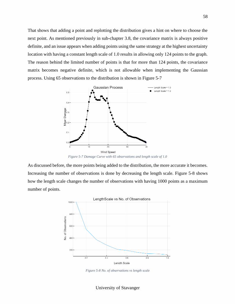
58


That shows that adding a point and replotting the distribution gives a hint on where to choose the

next point. As mentioned previously in sub-chapter 3.8, the covariance matrix is always positive

definite, and an issue appears when adding points using the same strategy at the highest uncertainty

location with having a constant length scale of 1.0 results in allowing only 124 points to the graph.

The reason behind the limited number of points is that for more than 124 points, the covariance

matrix becomes negative definite, which is not allowable when implementing the Gaussian

process. Using 65 observations to the distribution is shown in Figure 5-7

As discussed before, the more points being added to the distribution, the more accurate it becomes.

Increasing the number of observations is done by decreasing the length scale. Figure 5-8 shows

how the length scale changes the number of observations with having 1000 points as a maximum

number of points.

Figure 5-7 Damage Curve with 65 observations and length scale of 1.0

Figure 5-8 No. of observations vs length scale

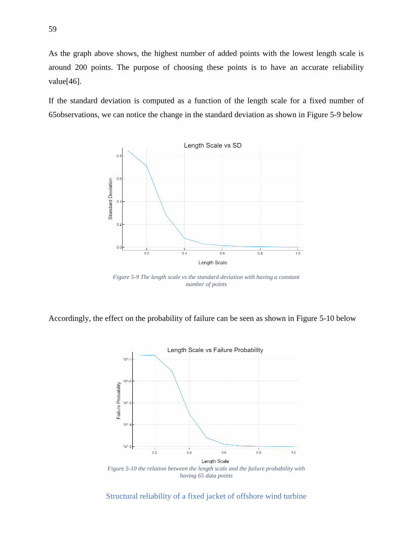
59


As the graph above shows, the highest number of added points with the lowest length scale is

around 200 points. The purpose of choosing these points is to have an accurate reliability

value[46].

If the standard deviation is computed as a function of the length scale for a fixed number of

65observations, we can notice the change in the standard deviation as shown in Figure 5-9 below

Accordingly, the effect on the probability of failure can be seen as shown in Figure 5-10 below

Figure 5-9 The length scale vs the standard deviation with having a constant

number of points

Figure 5-10 the relation between the length scale and the failure probability with

having 65 data points

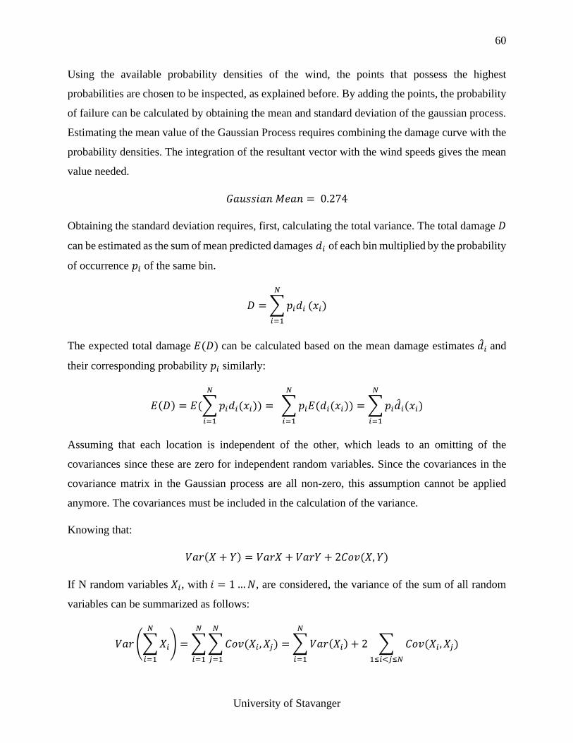
60


Using the available probability densities of the wind, the points that possess the highest

probabilities are chosen to be inspected, as explained before. By adding the points, the probability

of failure can be calculated by obtaining the mean and standard deviation of the gaussian process.

Estimating the mean value of the Gaussian Process requires combining the damage curve with the

probability densities. The integration of the resultant vector with the wind speeds gives the mean

value needed.

𝐺𝑎𝑢𝑠𝑠𝑖𝑎𝑛 𝑀𝑒𝑎𝑛 = 0.274

Obtaining the standard deviation requires, first, calculating the total variance. The total damage 𝐷

can be estimated as the sum of mean predicted damages 𝑑𝑖 of each bin multiplied by the probability

of occurrence 𝑝𝑖 of the same bin.

𝐷 =∑𝑝𝑖𝑑𝑖

𝑁

𝑖=1

(𝑥𝑖)

The expected total damage 𝐸(𝐷) can be calculated based on the mean damage estimates �̂�𝑖 and

their corresponding probability 𝑝𝑖 similarly:

𝐸(𝐷) = 𝐸(∑𝑝𝑖𝑑𝑖(𝑥𝑖

𝑁

𝑖=1

)) = ∑𝑝𝑖𝐸(𝑑𝑖(𝑥𝑖)

𝑁

𝑖=1

) =∑𝑝𝑖�̂�𝑖(𝑥𝑖)

𝑁

𝑖=1

Assuming that each location is independent of the other, which leads to an omitting of the

covariances since these are zero for independent random variables. Since the covariances in the

covariance matrix in the Gaussian process are all non-zero, this assumption cannot be applied

anymore. The covariances must be included in the calculation of the variance.

Knowing that:

𝑉𝑎𝑟(𝑋 + 𝑌) = 𝑉𝑎𝑟𝑋 + 𝑉𝑎𝑟𝑌 + 2𝐶𝑜𝑣(𝑋, 𝑌)

If N random variables 𝑋𝑖, with 𝑖 = 1…𝑁, are considered, the variance of the sum of all random

variables can be summarized as follows:

𝑉𝑎𝑟 (∑𝑋𝑖

𝑁

𝑖=1

) =∑∑𝐶𝑜𝑣(𝑋𝑖, 𝑋𝑗)

𝑁

𝑗=1

=∑𝑉𝑎𝑟(𝑋𝑖) + 2 ∑ 𝐶𝑜𝑣(𝑋𝑖, 𝑋𝑗)

1≤𝑖<𝑗≤𝑁

𝑁

𝑖=1

𝑁

𝑖=1

61


This leads to the variance of the total damage:

𝑉𝑎𝑟(𝐷) = 𝑉𝑎𝑟 (∑𝑝𝑖𝑑𝑖(𝑥𝑖)

𝑁

𝑖=1

) =∑∑𝐶𝑜𝑣(𝑝𝑖𝑑𝑖(𝑥𝑖), 𝑝𝑗𝑑𝑗(𝑥𝑗))

𝑁

𝑗=1

𝑁

𝑖=1

Knowing that:

𝐶𝑜𝑣(𝑋, 𝑌) = 𝐸(𝑋𝑌) − 𝐸(𝑋)𝐸(𝑌)

𝐸(𝑎𝑋) = 𝑎𝐸(𝑋)

𝐶𝑜𝑣(𝑎𝑋, 𝑏𝑌) = 𝐸(𝑎𝑋𝑏𝑌) − 𝐸(𝑎𝑋)𝐸(𝑏𝑌) = 𝑎𝑏𝐸(𝑋𝑌) − 𝑎𝑏𝐸(𝑋)𝐸(𝑌)

= 𝑎𝑏(𝐸(𝑋𝑌) − 𝐸(𝑋)𝐸(𝑌)) = 𝑎𝑏𝐶𝑜𝑣(𝑋, 𝑌)

This leads to:

𝑉𝑎𝑟(𝐷) =∑∑𝑝𝑖𝑝𝑗𝐶𝑜𝑣 (𝑑𝑖(𝑥𝑖), 𝑑𝑗(𝑥𝑗)) =

𝑁

𝑗=1

𝑁

𝑖=1

∑𝑝𝑖

𝑁

𝑖=1

∑𝑝𝑗𝐶𝑜𝑣 (𝑑𝑖(𝑥𝑖), 𝑑𝑗(𝑥𝑗))⏟ 𝐾𝑒𝑟𝑛𝑒𝑙 𝑓𝑢𝑛𝑐𝑡𝑖𝑜𝑛

𝑁

𝑗=1

Looking at the covariance matrix (e.g. for 𝑛 = 3), it can be seen that the above equation is the sum

of all covariance elements (multiplied with 𝑝𝑖 and 𝑝𝑗 respectively).

𝛴 = [

𝑉𝑎𝑟 𝑋1 𝐶𝑜𝑣(𝑋1, 𝑋2) 𝐶𝑜𝑣(𝑋1, 𝑋3)𝐶𝑜𝑣(𝑋2, 𝑋1) 𝑉𝑎𝑟 𝑋2 𝐶𝑜𝑣(𝑋2, 𝑋3)𝐶𝑜𝑣(𝑋3, 𝑋1) 𝐶𝑜𝑣(𝑋3, 𝑋2) 𝑉𝑎𝑟 𝑋3

]

The total variance is then:

𝑉𝑎𝑟(𝐷) = 1.44 ∗ 10−6

The standard deviation is calculated as the square root of the variance

𝐺𝑎𝑢𝑠𝑠𝑖𝑎𝑛 𝑆𝐷 = √𝑉𝑎𝑟(𝐷) = 0.0012

The probability of failure is calculated by integrating CDF of the log-normal and PDF of the

normal distribution of the gaussian mean and standard deviation.

𝐹𝑎𝑖𝑙𝑢𝑟𝑒 𝑃𝑟𝑜𝑏𝑎𝑏𝑖𝑙𝑖𝑡𝑦 (𝑃𝑓) = 1.0 ∗ 10−5

The reliability is then calculated as:

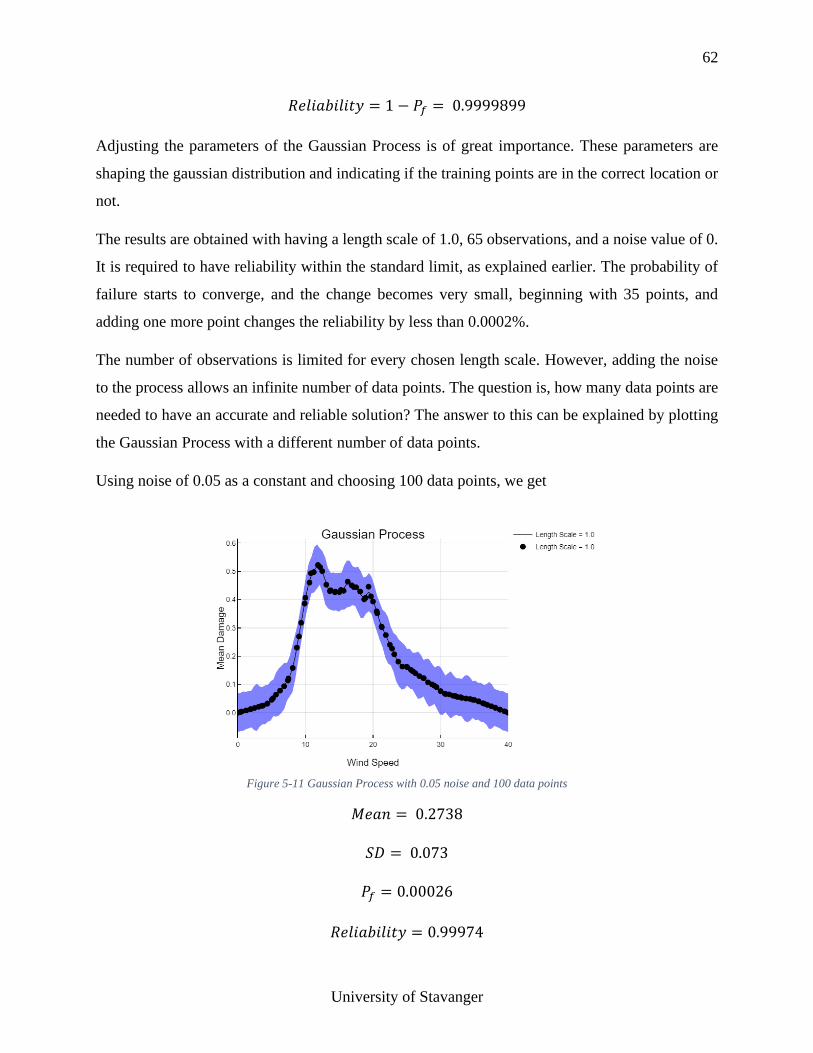
62


𝑅𝑒𝑙𝑖𝑎𝑏𝑖𝑙𝑖𝑡𝑦 = 1 − 𝑃𝑓 = 0.9999899

Adjusting the parameters of the Gaussian Process is of great importance. These parameters are

shaping the gaussian distribution and indicating if the training points are in the correct location or

not.

The results are obtained with having a length scale of 1.0, 65 observations, and a noise value of 0.

It is required to have reliability within the standard limit, as explained earlier. The probability of

failure starts to converge, and the change becomes very small, beginning with 35 points, and

adding one more point changes the reliability by less than 0.0002%.

The number of observations is limited for every chosen length scale. However, adding the noise

to the process allows an infinite number of data points. The question is, how many data points are

needed to have an accurate and reliable solution? The answer to this can be explained by plotting

the Gaussian Process with a different number of data points.

Using noise of 0.05 as a constant and choosing 100 data points, we get

𝑀𝑒𝑎𝑛 = 0.2738

𝑆𝐷 = 0.073

𝑃𝑓 = 0.00026

𝑅𝑒𝑙𝑖𝑎𝑏𝑖𝑙𝑖𝑡𝑦 = 0.99974

Figure 5-11 Gaussian Process with 0.05 noise and 100 data points

63


Using 200 data points, we get

𝑀𝑒𝑎𝑛 = 0.2739

𝑆𝐷 = 0.05

𝑃𝑓 = 7.95 ∗ 10−5


However, increasing the number of data points will reduce the failure probability and increase the

reliability until it converges to the same value obtained without the noise at about 500 observations.

Although the number of data points affects the standard deviation and the reliability, an alternative

solution is having constant data points and changing the noise. Reducing the noise and increasing



64


it changes the uncertainty of the distribution. If we have 100 data points and reduce the noise to

0.02, for instance, we get

𝑀𝑒𝑎𝑛 = 0.2739

𝑆𝐷 = 0.0292

𝑃𝑓 = 2.4 ∗ 10−5


This also shows that the change of noise influences the reliability as reducing the noise increases

the reliability, and decreasing it increases the reliability value.

If we have a constant number of data points, the standard deviation changes accordingly, as shown

in Figure 5-14 below

Figure 5-14 Relation between the noise and standard deviation with having 100

data points

Figure 5-15 Relation between the standard deviation and the no. of points with

having a constant noise of 0.05

65


Accordingly, if we have a fixed noise, for instance, of 0.05 and we change the number of

observations, we can notice the change of the standard deviation as shown in Figure 5-15 above.

Using the same comparison with the reliability instead of the standard deviation, for constant noise,

we can see the decrement of the probability of failure as shown in Figure 5-17 below

Similarly, we can see the change of the reliability with changing the noise while having a constant

number of data points, as shown in Figure 5-16 below

Figure 5-17 the relation between no. of points and the probability of failure with

having constant noise of 0.05

Figure 5-16 the relation between the noise and reliability with having 100 data

points

66


The above curves show how the number of observations differs by changing the hyperparameters

of the Gaussian Process. With the right choice of hyperparameters, one can reach the desired

results with the minimum number of observations. As explained earlier, if the noise is removed,

an accurate value of failure probability can be achieved using 35 points in the Gaussian

distribution. The exact value can be reached by adding slight noise and more than 500

observations. As the goal is to achieve the desired reliability with the minimum number of

observations, it would be more efficient and economical to use the method with fewer points.

67


Chapter 6: Discussion

Although the Gaussian Process has some challenges, the results obtained using this approach,

however, show that structural reliability can be obtained using a significantly small number of data

points instead of the hundreds and thousands of load-response simulations used in traditional

numerical methods. The challenge faced is the control of the hyperparameters of the Gaussian

Process together at the same time. Each of these parameters has an effect on the distribution of the

observations chosen.

6.1 Effect of Length Scale

The length scale showed how it could control the distribution from possessing high error or almost

zero error. Changing the length scale changes the number of observations and, consequently, the

shape of the distribution.

As explained in the previous chapter, the lower the length scale is, the more points can be added.

Having a small length scale with a low number of observations can lead to having a high failure

probability. It would be more accurate to have a constant length scale, 0.5, for instance, and keep

adding points until the results converge with the desired failure probability.

6.2 Effect of Noise

Although the noise, in a way, does not allow perfect fitting of the mean curve of the gaussian

distribution with the data points, it will enable adding as many data points as needed to estimate

the structure's accurate probability of failure and reliability. As shown in the results, the noise

Figure 6-1 Gaussian distribution with different length scales

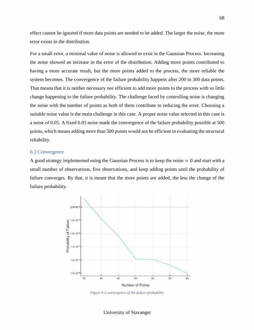
68


effect cannot be ignored if more data points are needed to be added. The larger the noise, the more

error exists in the distribution.

For a small error, a minimal value of noise is allowed to exist in the Gaussian Process. Increasing

the noise showed an increase in the error of the distribution. Adding more points contributed to

having a more accurate result, but the more points added to the process, the more reliable the

system becomes. The convergence of the failure probability happens after 200 to 300 data points.

That means that it is neither necessary nor efficient to add more points to the process with so little

change happening to the failure probability. The challenge faced by controlling noise is changing

the noise with the number of points as both of them contribute to reducing the error. Choosing a

suitable noise value is the main challenge in this case. A proper noise value selected in this case is

a noise of 0.05. A fixed 0.05 noise made the convergence of the failure probability possible at 500

points, which means adding more than 500 points would not be efficient in evaluating the structural

reliability.

6.3 Convergence

A good strategy implemented using the Gaussian Process is to keep the noise = 0 and start with a

small number of observations, five observations, and keep adding points until the probability of

failure converges. By that, it is meant that the more points are added, the less the change of the

failure probability.

Figure 6-2 convergence of the failure probability

69


As shown in Figure 6-2 above, the change in the failure probability is as low as 2 ∗ 10−6 every

five added points.

Eventually, comparing the Gaussian Process to the other deterministic methods shows that the

Gaussian Process achieves the desired results with significantly lower observations.

Table 6-1 Comparison between the different methods of obtaining the probability of failure

Bins Methos Monte Carlo

Integration

Numerical

Integration Gaussian Process

Number of

Points 1,000 1,000,000 10,000 65

Probability of

Failure 1 ∗ 10−5

Mean Damage 0.274

70


Chapter 7: Conclusion, Recommendation, and Further Work

The Gaussian Process is showing promising results in obtaining accurate fatigue reliability. With

fewer load-response simulations, it is possible to achieve the desired failure probability with a high

level of accuracy. Controlling the hyperparameters is the primary key to reaching the objective

required.

Comparing the Gaussian Process to other methods, such as Monte Carlo Integration, Bins method,

and Numerical Integration shows significant accuracy in the calculations with a significantly

smaller number of data points, which makes this approach efficient in terms of time consumption

and cost.

The Gaussian Process approach is performing, compared to the currently used methods in the

industry, relatively well. Challenges implementing the Gaussian Process, controlling the

hyperparameters, can be handled using efficient strategies.

7.1 Recommendations

7.1.1 Points Selection

A practical strategy is to start with defining the selected points of the Gaussian distribution. An

advantage of using the Gaussian Process is that it shows the variance in the distribution plot. The

highest variance value is the position of interest to add one more point to the distribution.

Replotting the distribution with the added point would show the following location to add more

points. This strategy helps to reduce the error significantly rather than choosing random points at

random locations of the distribution.

7.1.2 Convergence

Adding points lead to having more accurate results. A strategy to know where to stop adding points

or indicate having enough points would be the convergence of the probability of failure. If the

change in the likelihood of failure that occurs by adding points is too low, the process of adding

more points can be stopped.

A low difference is that the change is happening to the 4th or the 5th digit only. The convergence

value used in this thesis was 0.0001. Consequently, a change below this value indicates that adding

more points to the process is unnecessary.

71


7.2 Further Work

• Using a different type of hyperparameters optimization for more accuracy and efficiency.

• Using a different type of kernel function and how it would influence the whole Gaussian

process and the outputs.

• The Gaussian Process is implemented on one dimension, wind loading, in this thesis. It

would be exciting and beneficial to add another dimension, wave loading, for instance, to

the process and test its accuracy under different conditions.

72


References

[1] C. Zhu and Y. Li, Reliability Analysis of Wind Turbines. IntechOpen, 2018. doi:

10.5772/intechopen.74859.

[2] N. Jensen and C. WWF-Norway, “challenge: We need to contain global warming to hinder

catastrophic consequences for people and nature. Luckily we already know what needs to be

done: The global energy production needs to be shifted from fossil to renewable energy.

How we make this shift, will have everything to say for its success.,” p. 25.

[3] F. Fu, “Chapter Eight - Design of Offshore Structures,” in Design and Analysis of Tall and

Complex Structures, F. Fu, Ed. Butterworth-Heinemann, 2018, pp. 251–293. doi:

10.1016/B978-0-08-101018-1.00008-3.

[4] J. G. Speight, “Chapter 3 - Offshore Platforms,” in Subsea and Deepwater Oil and Gas

Science and Technology, J. G. Speight, Ed. Boston: Gulf Professional Publishing, 2015, pp.

71–106. doi: 10.1016/B978-1-85617-558-6.00003-9.

[5] C. Golightly, “Monopile and Tripod/Jacket Foundations for Offshore Wind Foundations

April 2014”, Accessed: May 01, 2021. [Online]. Available:

https://www.academia.edu/6952015/Monopile_and_Tripod_Jacket_Foundations_for_Offsho

re_Wind_Foundations_April_2014

[6] A. Taheri and G. Emamverdizadeh beyg, “Effect of Pile Scouring on the Structural Behavior

of a Fixed Jacket Platform with Consideration of Non-linear Pile Seabed Interaction,” J.

Rehabil. Civ. Eng., no. Online First, Sep. 2017, doi: 10.22075/jrce.2017.12150.1206.

[7] L. Drummond, M. Mulcahy, and S. Culloty, “The reproductive biology of the Manila clam,

Ruditapes philippinarum, from the North-West of Ireland,” Aquaculture, vol. 254, no. 1, pp.

326–340, Apr. 2006, doi: 10.1016/j.aquaculture.2005.10.052.

[8] A. Lapworth, “The diurnal variation of the marine wind in an offshore flow,” Q. J. R.

Meteorol. Soc., vol. 131, pp. 2367–2387, Dec. 2006, doi: 10.1256/qj.04.161.

[9] Ö. Halici and H. Mutungi, “Assessment of simulation codes for offshore wind turbine

foundations,” 2016.

[10] P. S. Maran, “Meteorological tower wind shear characteristics, vertical wind speed

profile, and surface roughness analysis near the coastline of Chennai,” p. 6, 2019.

[11] E. Petersen, N. Mortensen, L. Landberg, and H. Frank, “Wind Power Meteorology,” Jan.

1997.

73


[12] A. Abdalla, W. El-Osta, and E. Dekam, The Influence Of The Atmospheric Stability

Conditions On The Available Wind Energy For Three Libyan coastal Cities. 2017.

[13] M. L. Hossain, A. Abu-Siada, and S. M. Muyeen, “Methods for Advanced Wind Turbine

Condition Monitoring and Early Diagnosis: A Literature Review,” Energies, vol. 11, no. 5,

Art. no. 5, May 2018, doi: 10.3390/en11051309.

[14] E. L. Petersen, 1999 European Wind Energy Conference: Wind Energy for the Next

Millennium. Routledge, 2014.

[15] B. Hahn, M. Durstewitz, and K. Rohrig, “Reliability of wind turbines: Experiences of 15

years with 1,500 WTs,” Fraunhofer IWES, Jan. 2006.

[16] S. Faulstich, B. Hahn, and P. J. Tavner, “Wind turbine downtime and its importance for

offshore deployment,” Wind Energy, vol. 14, Apr. 2011, doi: 10.1002/we.421.

[17] J. Linsday, D. Briand, R. R. Hill, J. A. Stinebaugh, and A. S. Benjamin, “Wind turbine

reliability : a database and analysis approach.,” SAND2008-0983, 1028916, Feb. 2008. doi:

10.2172/1028916.

[18] B. H. Chudnovsky, Transmission, Distribution, and Renewable Energy Generation

Power Equipment: Aging and Life Extension Techniques, Second Edition. CRC Press, 2017.

[19] D. S. Saini, D. Karmakar, and S. ray chaudhuri, “A Review of Stress Concentration

Factors in Tubular and Non-Tubular Joints for Design of Offshore Installations,” J. Ocean

Eng. Sci., vol. 1, Aug. 2016, doi: 10.1016/j.joes.2016.06.006.

[20] B. Yong and J. Wei-Liang, Marine Structural Design. Elsevier, 2016. doi:

10.1016/C2013-0-13664-1.

[21] S. W. Smith, The scientist and engineer’s guide to digital signal processing. San Diego,

Calif.: California Technical Pub., 1999.

[22] J. V. Kemble, “PH changes on the surface of burns,” Br. J. Plast. Surg., vol. 28, no. 3, pp.

181–184, Jul. 1976, doi: 10.1016/0007-1226(75)90126-5.

[23] H. Holzer, “Chemistry and biology of macromolecular inhibitors from yeast acting on

proteinases A and B, and carboxypeptidase Y,” Adv. Enzyme Regul., vol. 13, pp. 125–134,

1974, doi: 10.1016/0065-2571(75)90011-4.

[24] H. R. Maier, B. J. Lence, B. A. Tolson, and R. O. Foschi, “First-order reliability method

for estimating reliability, vulnerability, and resilience,” Water Resour. Res., vol. 37, no. 3,

pp. 779–790, Mar. 2001, doi: 10.1029/2000WR900329.

74


[25] A. Halder and S. Mahadevan, “Probability, Reliability, and Statistical Methods in

Engineering Design | Wiley,” Wiley.com. https://www.wiley.com/en-

us/Probability%2C+Reliability%2C+and+Statistical+Methods+in+Engineering+Design-p-

9780471331193 (accessed Jun. 14, 2021).

[26] S. Maskey and V. Guinot, “Improved first-order second moment method for uncertainty

estimation in flood forecasting,” Hydrol. Sci. JournalJournal Sci. Hydrol., vol. 48, pp. 183–

196, Apr. 2003, doi: 10.1623/hysj.48.2.183.44692.

[27] R. E. Melchers and A. T. Beck, Structural reliability analysis and prediction, Third

edition. Hoboken, NJ: Wiley, 2018.

[28] “DNVGL-OS-C101.pdf.” Accessed: Apr. 30, 2021. [Online]. Available:

https://rules.dnvgl.com/docs/pdf/dnvgl/os/2015-07/DNVGL-OS-C101.pdf

[29] B. Liu and L. Xie, “An Improved Structural Reliability Analysis Method Based on Local

Approximation and Parallelization,” Mathematics, vol. 8, no. 2, p. 209, Feb. 2020, doi:

10.3390/math8020209.

[30] H. Zhang, H. Dai, M. Beer, and W. Wang, “Structural reliability analysis on the basis of

small samples: An interval quasi-Monte Carlo method,” Mech. Syst. Signal Process., vol. 37,

pp. 137–151, May 2013, doi: 10.1016/j.ymssp.2012.03.001.

[31] H. Ray, “Sturge’s Rule; A Method for Selecting the Number of Bins in a Histogram,”

Accendo Reliability, Aug. 11, 2020. https://accendoreliability.com/sturges-rule-method-

selecting-number-bins-histogram/ (accessed Jun. 04, 2021).

[32] V. Cumer, “The basics of Monte Carlo integration,” Medium, Nov. 06, 2020.

https://towardsdatascience.com/the-basics-of-monte-carlo-integration-5fe16b40482d

(accessed Jun. 05, 2021).

[33] M Muskulus and S Schafhirt, “Reliability-based design of wind turbine support

structures,” 2015, doi: 10.13140/RG.2.1.5125.5766.

[34] H. Li, Y. He, and X. Nie, “Structural reliability calculation method based on the dual

neural network and direct integration method,” Neural Comput. Appl., vol. 29, no. 7, pp.

425–433, Apr. 2018, doi: 10.1007/s00521-016-2554-7.

[35] A. Francisco, J. A. Duran, C. Vilela, and T. Simões, Comparison of Numerical

Integration and Monte Carlo Simulation Methods for Structural Reliability based on the

Failure Assessment Diagram. 2015. doi: 10.20906/CPS/CILAMCE2015-0416.

75


[36] J. Görtler, R. Kehlbeck, and O. Deussen, “A Visual Exploration of Gaussian Processes,”

Distill, vol. 4, no. 4, p. e17, Apr. 2019, doi: 10.23915/distill.00017.

[37] S. Yuge, “Gaussian Processes, not quite for dummies,” The Gradient, Nov. 13, 2019.

https://thegradient.pub/gaussian-process-not-quite-for-dummies/ (accessed Jun. 10, 2021).

[38] D. Baccanari, A. Phillips, S. Smith, D. Sinski, and J. Burchall, “Purification and

properties of Escherichia coli dihydrofolate reductase,” Biochemistry, vol. 14, no. 24, pp.

5267–5273, Dec. 2015, doi: 10.1021/bi00695a006.

[39] J. Butler, G. G. Jayson, and A. J. Swallow, “The reaction between the superoxide anion

radical and cytochrome c,” Biochim. Biophys. Acta, vol. 408, no. 3, pp. 215–222, Dec. 2016,

doi: 10.1016/0005-2728(75)90124-3.

[40] A. Schmoldt, H. F. Benthe, and G. Haberland, “Digitoxin metabolism by rat liver

microsomes,” Biochem. Pharmacol., vol. 24, no. 17, pp. 1639–1641, Sep. 2017.

[41] L. Kang, R.-S. Chen, N. Xiong, Y.-C. Chen, Y.-X. Hu, and C.-M. Chen, “Selecting

Hyper-Parameters of Gaussian Process Regression Based on Non-Inertial Particle Swarm

Optimization in Internet of Things,” IEEE Access, vol. 7, pp. 59504–59513, 2019, doi:

10.1109/ACCESS.2019.2913757.

[42] S. Bartels and P. Hennig, “Conjugate Gradients for Kernel Machines,” p. 42.

[43] G. Su, J. Jiang, B. Yu, and Y. Xiao, “A Gaussian process-based response surface method

for structural reliability analysis,” Struct. Eng. Mech., vol. 56, pp. 549–567, Nov. 2015, doi:

10.12989/sem.2015.56.4.549.

[44] C. E. Rasmussen and C. K. I. Williams, Gaussian processes for machine learning.

Cambridge, Mass: MIT Press, 2006.

[45] Z. Daniel and M. Michael, “Simplified fatigue load assessment in offshore wind turbine

structural analysis”, doi: 10.1002/we.1831.

[46] G. Sigurdsson, E. Cramer, I. Lotsberg, B. Berge, and Ø. Hagen, “Guideline for Offshore

Structural Reliability,” Tech. Rep., no. 95, p. 80.

76


Appendix

Julia Script

This script is written using Julia version 1.5.3.

using NumericalIntegration

using QuadGK

using Distributions

import Random: randn, MersenneTwister

# Probability density function for the wind

"""

Weibull(beta,eta,gamma,x)

Returns the Weibull distribution for `x`.

`beta` ... Shape parameter (or slope)

`eta` ... Scale parameter

`gamma` ... Location parameter; frequently not used

"""

function weibull( beta::AbstractFloat,

eta::AbstractFloat,

gamma::AbstractFloat,

x::Array{<:AbstractFloat,1})

return beta/eta*((x.-gamma)/eta).^(beta-1).*exp.(-((x.-gamma)/eta).^beta)

end

# version for x as Float64

function weibull( beta::AbstractFloat,

eta::AbstractFloat,

gamma::AbstractFloat,

x::AbstractFloat)

return weibull(beta, eta, gamma, [x])[1]

end

# Parameter for the Upwind Deepwater-Site

beta = 2.04

eta = 11.75

gamma = 0.0

# Define wind distribution function as function depending only on wind speed v

77


upwindDistr(v) = weibull(beta,eta,gamma,v)

"""

linearInterpolation(xarray, yarray, interpolateX)

Linear interpolation between two values.

# Example

```julia-repl

julia> linearInterpolation([1, 2], [0, 4], 1.5)

2.0

```

"""

function linearInterpolation(xarray::Array{Float64,1},yarray::Array{Float64,1},

interpolateX::Float64)

minX, maxX = minimum(xarray), maximum(xarray)

# Check argument in bounds

minX <= interpolateX <= maxX || error("Input value out of bounds, no interpola

tion possible!")

interpolateX == maxX && return yarray[end]

# Location in array which is below interpolation value

loc1 = findall(x -> x<=interpolateX, xarray)[end]

# Linear interpolation

x1, x2 = xarray[loc1], xarray[loc1+1]

y1, y2 = yarray[loc1], yarray[loc1+1]

return interpolateY = (interpolateX-x1)/(x2-x1)*(y2-y1)+y1

end

# Version for Array input


interpolateX::Array{Float64,1})

interpolateY = Float64[]

for i in interpolateX

push!(interpolateY, linearInterpolation(xarray,yarray,i))

end

return interpolateY

end

# Int version

78



interpolateX::Int64)

return linearInterpolation(xarray, yarray, Float64(interpolateX))

end

"""

createDamageData()

Generates the artifical damage results for wind speeds between 0 and 40 m/s.

- returns 2 1D arrays: windVelocity and damage

"""

function createDamageData(;deltaV = 0.05, noiseRatio = 0.025)

# Raw data from Zwick, Muskulus

# Simplified fatigue load assessment in offshore wind turbine structural analy

sis

# Figure 3 - level 5

rawdata = [

# Linear assumption to zero velocity

0.0 0.0;

# Data from paper

3.99304 0.00761;

5.00209 0.01269;

6.00418 0.02081;

7.00626 0.02690;

7.99443 0.04061;

8.99652 0.07310;

9.99861 0.11472;

11.0007 0.14112;

12.0027 0.14365;

13.0048 0.12995;

14.0069 0.12132;

# artifical peak #1

14.2000 0.14021;

14.3000 0.11903;

# end

14.9951 0.12030;

15.9972 0.12335;

79


16.9993 0.12843;

19.0034 0.11168;

# artifical peak #2

19.2000 0.13579;

19.3000 0.12403;

# end

20.9937 0.08985;

24.0069 0.04924;

# made up data for higher wind speeds

29.0 0.02690;

30.0000 0.02081;

# artifical peak #3

30.2000 0.03021;

30.3000 0.01903;

# end

35.0000 0.01269;

40.0000 0.00000]

rawdata[:,2] = rawdata[:,2]*3.554648550953938

# Add noise

# Random number generator with constant seed

rng = MersenneTwister(123456);

# Wind speed array

# from 0 m/s to 40 m/s, every 0.05 m/s

windVelocity = collect(0:deltaV:40)

l=length(windVelocity)

damages = Float64[]

for i in windVelocity

velocity = linearInterpolation(rawdata[:,1],rawdata[:,2],i)

noise = noiseRatio*velocity*randn(rng)

push!(damages,velocity+noise)

end

80


return windVelocity, damages

end

# example plot of wind distribution and damage data

import Plots

# Generate the wind velocity and damage arrays

v, d =createDamageData();

# Generate the Weibull PDF for the given wind velocity array

p = upwindDistr(v);

p1 = Plots.plot(v,p, xlabel="wind speed [m/s]", label="Weibull distribution", lw=

2, linecolor = :black)

p2 = Plots.plot(v,d, xlabel="wind speed [m/s]", label="Damage curve", lw=2)

Plots.plot(p1, p2, layout=(2,1))

# 2020-03-10: Additional linearInterpolation posibilities

# getting return value inbetween two values, x as Float64

linearInterpolation(v,d,3.12341234)

# getting return value inbetween two values, x as Int64

linearInterpolation(v,d,3)

# getting return value inbetween two values, x as Array of Floats

linearInterpolation(v,d,[3.12341234, 17.12334, 33.12])

#damage with bins

using Distributions

using QuadGK

function BinsDam(N)

step = floor(Int, length(v)/N) #defining the step between each point

speed = v[1:step:end]

speed2=Float64[]

Pdf=[] #empty array to push in the probabilities

for i in 1:N

spd = (speed[i]+speed[i+1])/2

push!(speed2 , spd)

end

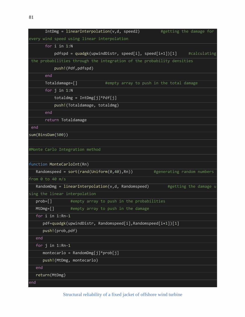
81


IntDmg = linearInterpolation(v,d, speed2) #getting the damage for

every wind speed using linear interpolation

for i in 1:N

pdfspd = quadgk(upwindDistr, speed[i], speed[i+1])[1] #calculating

the probabilities through the integration of the probability densities

push!(Pdf,pdfspd)

end

Totaldamage=[] #empty array to push in the total damage

for j in 1:N

totaldmg = IntDmg[j]*Pdf[j]

push!(Totaldamage, totaldmg)

end

return Totaldamage

end

sum(BinsDam(500))

#Monte Carlo Integration method

function MonteCarloInt(Rn)

Randomspeed = sort(rand(Uniform(0,40),Rn)) #generating random numbers

from 0 to 40 m/s

RandomDmg = linearInterpolation(v,d, Randomspeed) #getting the damage u

sing the linear interpolation

prob=[] #empty array to push in the probabilities

MtDmg=[] #empty array to push in the damage

for i in 1:Rn-1

pdf=quadgk(upwindDistr, Randomspeed[i],Randomspeed[i+1])[1]

push!(prob,pdf)

end

for j in 1:Rn-1

montecarlo = RandomDmg[j]*prob[j]

push!(MtDmg, montecarlo)

end

return(MtDmg)

end

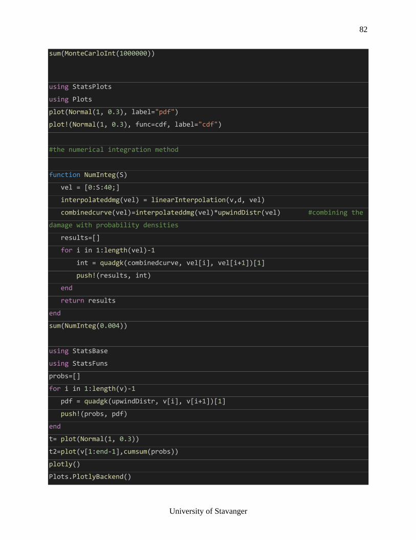
82


sum(MonteCarloInt(1000000))

using StatsPlots

using Plots

plot(Normal(1, 0.3), label="pdf")

plot!(Normal(1, 0.3), func=cdf, label="cdf")

#the numerical integration method

function NumInteg(S)

vel = [0:S:40;]

interpolateddmg(vel) = linearInterpolation(v,d, vel)

combinedcurve(vel)=interpolateddmg(vel)*upwindDistr(vel) #combining the

damage with probability densities

results=[]

for i in 1:length(vel)-1

int = quadgk(combinedcurve, vel[i], vel[i+1])[1]

push!(results, int)

end

return results

end

sum(NumInteg(0.004))

using StatsBase

using StatsFuns

probs=[]

for i in 1:length(v)-1

pdf = quadgk(upwindDistr, v[i], v[i+1])[1]

push!(probs, pdf)

end

t= plot(Normal(1, 0.3))

t2=plot(v[1:end-1],cumsum(probs))

plotly()

Plots.PlotlyBackend()

83


miuD = -0.0431 #miu of the log-normal

sigmaD = 0.2935 #sigma of the log-normal

plot(LogNormal(miuD, sigmaD), func= cdf)

roll=LogNormal(miuD, sigmaD)

plot(roll , label="Lognormal PDF")

vline!([0.278], label="determinitsic damage")

Pf = quadgk(x->pdf(roll,x), 0,sum(NumInteg(0.004)))[1]

reliability = 1-Pf

using GaussianProcesses

import LinearAlgebra: diag

R=Float64[0.0, 10.0, 20.0, 30.0, 40.0] #array with the initially chos

en points

#a function to generate the data of the gaussian process

function gendata(x)

y= linearInterpolation(v,d,x)

kernel=SE(log(1.0),log(1.0)) #the kernel function of the gaussian proce

ss

Mean=MeanZero()

LogNoise = log(0.05)

gaussianprocess= GP(x, y, Mean, kernel, LogNoise)

rangeval = range(0,stop=40,length=1000) #dividing the wind speed into 100

0 segments

rangevalue = [0.0:0.04004004004004004:40.0;]

meanval, CoVmatrix = predict_f(gaussianprocess,rangeval;full_cov=true);

varval = abs.(diag(CoVmatrix))

return meanval, varval, rangevalue, sum(CoVmatrix)

end

84


#function to locate the maximum variance value in the gaussian distribution

function Locatevar(wind,Var)

return wind[findmax((Var)[1:end])[2]]

end

#function to add the point corresponding to the maximum variance to the initially

selected points (R)

function Addingpt(R, newlocation)

G = push!(R,newlocation)

return sort(G)

end

#a function collecting the previous three functions to generate the points automa

tically into "R" array

function DataPoints(s)

R=sort(R)

Mean,Var,wind,totVar=gendata(R)

Maxvarpt=Locatevar(wind,Var)

Addingpt(R,Maxvarpt)

return R

end

DataPoints(R)

#Function to calculate the Gaussian Process reliability

function GaussianRel(z,v,d)

y= linearInterpolation(v,d,z) #linear interpolation to calcula

te the damage at the chosen wind speeds

kernel=SE(log(1.0),log(1.0)) #Kernel function of the Gaussian

Process

Mean=MeanZero() #mean function of the Gaussian P

rocess

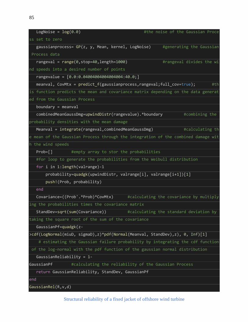
85


LogNoise = log(0.0) #the noise of the Gaussian Proce

ss set to zero

gaussianprocess= GP(z, y, Mean, kernel, LogNoise) #generating the Gaussian

Process data

rangeval = range(0,stop=40,length=1000) #rangeval divides the wi

nd speeds into a desired number of points

rangevalue = [0.0:0.04004004004004004:40.0;]

meanval, CovMtx = predict_f(gaussianprocess,rangeval;full_cov=true); #th

is function predicts the mean and covariance matrix depending on the data generat

ed from the Gaussian Process

boundary = meanval

combinedMeanGaussDmg=upwindDistr(rangevalue).*boundary #combining the

probability densities with the mean damage

Meanval = integrate(rangeval,combinedMeanGaussDmg) #calculating th

e mean of the Gaussian Process through the integration of the combined damage wit

h the wind speeds

Prob=[] #empty array to stor the probabilities

#for loop to generate the probabilities from the Weibull distribution

for i in 1:length(valrange)-1

probability=quadgk(upwindDistr, valrange[i], valrange[i+1])[1]

push!(Prob, probability)

end

Covariance=((Prob'.*Prob)*CovMtx) #calculating the covariance by multiply

ing the probabilities times the covariance matrix

StandDev=sqrt(sum(Covariance)) #calculating the standard deviation by

taking the square root of the sum of the covariance

GaussianPf=quadgk(z-

>cdf(LogNormal(miuD, sigmaD),z)*pdf(Normal(Meanval, StandDev),z), 0, Inf)[1]

# estimating the Gaussian failure probability by integrating the cdf function

of the log-normal with the pdf function of the gaussian normal distribution

GaussianReliability = 1-

GaussianPf #calculating the reliability of the Gaussian Process

return GaussianReliability, StandDev, GaussianPf

end

GaussianRel(R,v,d)

86


#Gaussian plot function

function GaussianPlot(z)

y= linearInterpolation(v,d,z)

kernel=SE(log(1.0),log(1.0))

Mean=MeanZero()

LogNoise = log(0.0)

gaussianprocess= GP(z, y, Mean, kernel, LogNoise)

gauplot = plot(gaussianprocess, xlabel="Wind Speed", ylabel="Mean Damage", tit

le="Gaussian Process", label="Length Scale = 1.0", fillcolor = :green)

return gauplot

end

GaussianPlot(R)