structural performance of low grade timber slabs
TRANSCRIPT

University of Southern Queensland
Faculty of Engineering and Surveying
Structural Performance of Low Grade Timber Slabs
A dissertation submitted by
Cameron James Clifford Summerville
In fulfilment of the requirements of
Courses ENG 4111 and ENG4112 Research Project
Towards the degree of
Bachelor of Engineering (Civil Engineering)
Submitted: October 2009

i
Faculty of Engineering and Surveying
ENG4111 & ENG4112 Research Project
Limitations of Use
The Council of the University of Southern Queensland, its Faculty of
Engineering and Surveying, and the staff of the University of Southern
Queensland, do not accept any responsibility for the truth, accuracy or
completeness of material contained within or associated within or
associated with this dissertation.
Persons using all or any part of this material do so at their own risk, and not
at the risk of the Council of the University of Southern Queensland, its
Faculty of Engineering and Surveying or the staff of the University of
Southern Queensland.
This dissertation reports an educational exercise and has no purpose or
validity beyond this exercise. The sole purpose of the course pair entitled
“Research Project” is to contribute to the overall education within the
student‟s chosen degree program. This document, the associated hardware,
software, drawings and other material set out in the associated appendices
should not be used for any other purpose: if they are so used, it is entirely at
the risk of the user.
Prof Frank Bullen
Dean
Faculty of Engineering and Surveying

ii
Certification
I certify that the ideas, designs and experimental work, results, analyses
and conclusions set out in this dissertation are entirely my own effort,
except where otherwise indicated and acknowledged.
I further certify that the work is original and has not been previously
submitted for assessment in any other course or institution, except where
specifically stated.
Cameron James Clifford Summerville
Student Number: 0050057183
______________________________________
Signature
______________________________________
Date

iii
Abstract
Low grade pine subject to loading exhibits a poor predictability when used
in structural applications. Australia produces a large amount of low grade
timber yearly which is sold at a loss due to its unreliable performance
characteristics. This dissertation investigates the structural performance of
slab units manufactured from low grade timber when used to form a floor
slab.
Physical testing and finite element analysis modelling have been used to
determine the limitations of low grade timber floor slabs. This study
involved determining which of the strength and serviceability criteria
governs design, along with an investigation into the performance of bugle
head batten screws used to connect low grade slab units to form a floor
slab. The findings of these investigations are summarised into a chart for
the deflection based design of low grade timber floor slabs, and graphs
describing connection performance based on various loading situations.
Investigations have concluded that utilising low grade timber in floor units
increases the reliability of the product considerably. Connections can also
be made that have sufficient strength to resist any forces applied between
slab units.

iv
Acknowledgments
I would like to thank everyone who has assisted me in any form throughout
the time spent doing this research. In particular I would like to make a
special mention of:
My family for their continued support in all of my endeavours.
Associate Professor Karu Karunasena for the valuable guidance he
has provided to me as my research supervisor.
Geoff Stringer from Hyne and son for sponsoring this research,
providing materials, data and valuable industry expertise when
needed.
Colin MacKenzie from Timber Queensland for the provision of
hardwood test data required for comparative modelling, and expert
industry knowledge as required,
Wayne Crowell, Mohan Trada, Daniel Eising and Joseph Marstella
for their assistance in testing.
I am very grateful for the input and assistance provided by these people.
Cameron J.C Summerville
University of Southern Queensland
October 2009

v
Table of Contents
ABSTRACT ....................................................................................................................................... III
ACKNOWLEDGMENTS.................................................................................................................. IV
LIST OF FIGURES ........................................................................................................................ VIII
LIST OF TABLES ............................................................................................................................... X
NOMENCLATURE ........................................................................................................................... XI
1 INTRODUCTION ............................................................................................................................ 1
1.0 OUTLINE OF THE STUDY ...................................................................................................... 1
1.1 BACKGROUND ..................................................................................................................... 2
1.2 THE PROBLEM .................................................................................................................... 3
1.3 RESEARCH OBJECTIVES ...................................................................................................... 5
1.4 OVERVIEW OF THE DISSERTATION ...................................................................................... 6
2 LITERATURE REVIEW ................................................................................................................. 7
2.0 INTRODUCTION ................................................................................................................... 7
2.1 USE OF GLULAM TECHNOLOGY .......................................................................................... 8
2.2 TIMBER MATERIAL PROPERTIES ........................................................................................10
2.3 CURRENT TIMBER FLOORING PRACTICE ............................................................................10
2.4 STANDARD FLOOR LOADING AND DESIGN ...........................................................................11
2.5 TIMBER ELEMENT MODELLING ..........................................................................................11
2.6 CURRENT TIMBER SLAB CONSTRUCTION PRACTICE ...........................................................12
2.7 RELEVANT AUSTRALIAN STANDARDS ................................................................................13
2.8 SUMMARY ..........................................................................................................................13
3 INDIVIDUAL MEMBER STRENGTH TESTING ........................................................................15
3.0 INTRODUCTION ..................................................................................................................15
3.1 METHODOLOGY .................................................................................................................17
3.2 RESULTS ............................................................................................................................20
3.3 DISCUSSION .......................................................................................................................23
3.4 CONCLUSIONS ....................................................................................................................24
4 LOW GRADE SLAB STRENGTH TESTING ...............................................................................25
4.0 INTRODUCTION ..................................................................................................................25
4.1 METHODOLOGY .................................................................................................................27
4.2 RESULTS ............................................................................................................................30

vi
4.3 DISCUSSION .......................................................................................................................33
4.4 CONCLUSIONS ....................................................................................................................35
5 FINITE ELEMENT ANALYSIS .....................................................................................................37
5.0 INTRODUCTION ..................................................................................................................37
5.1 SELECTION AND JUSTIFICATION OF APPROPRIATE MODELLING PARAMETERS. ..................39
5.1.1 One dimensional beam element model ........................................................................40
5.1.2 Two dimensional plate element model .........................................................................42
5.1.3 Three dimensional brick element model ......................................................................44
5.1.4 Use of isotropic elements ..............................................................................................45
5.1.5 Application and justification of chosen poisons ratio ..................................................47
5.2 METHODOLOGY .................................................................................................................49
5.2.1 Parametric study between slab and standard flooring ................................................52
5.2.2 Modelling of slab performance to create design chart ................................................57
5.3 RESULTS ............................................................................................................................59
5.3.1 Parametric study between slab and standard flooring ................................................62
5.3.2 Low grade timber slab design chart ............................................................................63
5.4 DISCUSSION .......................................................................................................................65
5.4.1 Parametric study between slab and standard flooring. ...............................................66
5.4.2 Low grade timber slab design chart. ...........................................................................67
5.5 CONCLUSIONS ....................................................................................................................69
6 CONNECTIONS ..............................................................................................................................71
6.0 INTRODUCTION ..................................................................................................................71
6.1 METHODOLOGY .................................................................................................................73
6.1.1 Connection methods evaluation ...................................................................................73
6.1.2 Selection using weighted decision matrix ....................................................................74
6.1.3 Bugle head batten screw testing methodology .............................................................78
6.1.3.1 Two slab bending test ...................................................................................................... 78
6.1.3.2 Three slab shear and bending test ................................................................................... 79
6.1.3.3 Batten screw shear capacity testing ................................................................................. 81
6.1.3.4 Individual member shear capacity testing ....................................................................... 83
6.1.3.5 Three slab pure shear test ................................................................................................ 85
6.2 RESULTS ............................................................................................................................87
6.2.1 Two slab bending test ...................................................................................................88
6.2.2 Three slab shear and bending test ...............................................................................90
6.2.3 Batten screw shear capacity testing .............................................................................92
6.2.4 Individual member shear capacity testing ...................................................................93
6.2.5 Three slab pure shear test ............................................................................................96
6.3 DISCUSSION .......................................................................................................................98
6.3.1 Combined actions testing. .......................................................................................... 100
6.3.2 Batten screw shear capacity testing ........................................................................... 102
6.3.3 Individual member shear capacity testing ................................................................. 103

vii
6.3.4 Three slab pure shear test. ......................................................................................... 104
6.4 CONCLUSIONS .................................................................................................................. 107
7 CONCLUSIONS ............................................................................................................................ 108
7.0 SUMMARY ........................................................................................................................ 108
7.1 ACHIEVEMENT OF PROJECT OBJECTIVES ......................................................................... 109
7.2 MAJOR FINDINGS ............................................................................................................. 112
7.3 FUTURE WORK ................................................................................................................ 113
LIST OF REFERENCES ................................................................................................................. 115
APPENDIX A – PROJECT SPECIFICATION ............................................................................... 118
APPENDIX B – OH&S – WORK PERMIT .................................................................................... 120
APPENDIX C – OH&S – PURBOND 514 MSDS ............................................................................ 128
APPENDIX D – HYNE TUAN MILL MATERIAL PROPERTY DATA ....................................... 126
APPENDIX E – TIMBER QUEENSLAND GREY IRONBARK TEST DATA ............................. 128
APPENDIX F – SLAB UNIT CONNECTION IDEAS .................................................................... 132
APPENDIX G – MATLAB CODE USED TO ANALYSE RECORDED DATA ............................ 136
G.1 – MATLAB CODE USED TO PLOT TEST RESULTS. ...................................................................... 137
G.2 – MATLAB CODE USED TO CALCULATE MODULUS OF ELASTICITY .......................................... 140
G.3 – MATLAB CODE USED TO PLOT DESIGN CHART ...................................................................... 141
G.4 – MATLAB CODE USED TO PLOT STRESS LIMIT GRAPHS .......................................................... 143
G.5 – MATLAB CODE USED TO PLOT DEFLECTION LIMIT GRAPHS .................................................. 151

viii
List of Figures
Figure 1 – Loading Setup.......................................................................................... 17
Figure 2 – Testing of an individual low grade timber member. .............................. 18
Figure 3 – A combination of knot and resin shake failure ...................................... 20
Figure 4 – Test results obtained from individual low grade timber members. ...... 21
Figure 5 – Individual low grade timber members after destructive testing. .......... 22
Figure 6 – Failure modes based on the location of major defects. .......................... 23
Figure 7 – Slab unit cross section ............................................................................. 26
Figure 8 – Sample specimens prior to testing .......................................................... 28
Figure 9 – Slab testing setup. .................................................................................... 29
Figure 10 – Low grade slab partial failure. .............................................................. 30
Figure 11 – Low grade timber slab test results. ....................................................... 32
Figure 12 – Random distribution of knots and defect free sections ........................ 33
Figure 13 – Alignment of defects within a slab. ....................................................... 34
Figure 14 – Floor construction configurations......................................................... 38
Figure 15 – A one dimensional beam element model. .............................................. 40
Figure 16 – Comparison between one dimensional model and physical results. .... 41
Figure 17 – A two dimensional plate element model. .............................................. 42
Figure 18 – Node location within a two dimensional slab model cross section ....... 43
Figure 19 – A three dimensional brick element model. ........................................... 44
Figure 20 – Node location within a three dimensional slab model cross section. ... 45
Figure 21 – Comparison of Strand7 models to physical test results ....................... 46
Figure 22 – Derivation of maximum moment from loading setup. ......................... 49
Figure 23 – Stress distribution within the slab. ....................................................... 50
Figure 24 – Standard floor construction Strand7 model ......................................... 54
Figure 25 – Supports used in Strand7 floor models................................................. 55
Figure 26 – Low grade timber slab floor Strand7 model ........................................ 55
Figure 27 – Strand7 load case combination screen print. ....................................... 58
Figure 28 – 3.6m span deflection limit graph for both floor model types. .............. 60
Figure 29 – 3.6m span stress limit graph for both floor model types ...................... 60
Figure 30 – 6m span deflection limit graph for both floor types ............................. 61
Figure 31 – 6m span stress limit graph for both floor types .................................... 61
Figure 32 – Comparison between a standard and a low grade timber slab floor. .. 62

ix
Figure 33 – Low grade timber slab design chart. .................................................... 64
Figure 34 – Cross section of chosen connection method .......................................... 75
Figure 35 – Arrangement of bugle head batten screws. .......................................... 76
Figure 36 – Creating the correct angle for the screw joint. ..................................... 77
Figure 37 – Plan view of chosen connection system ................................................. 77
Figure 38 – Loading setup for two slab bending test. .............................................. 78
Figure 39 – Loading setup used on three slab test shear and bending test. ............ 80
Figure 40 – Batten screw shear testing rig ............................................................... 82
Figure 41 – MTS machine used for testing the bugle head batten screws .............. 82
Figure 42 – Supports used in the individual member shear tests ............................ 83
Figure 43 – Setting up the individual member shear capacity test. ........................ 84
Figure 44 – Testing setup used for the three slab pure shear test. .......................... 85
Figure 45 – Supports used in three slab pure shear test. ......................................... 86
Figure 46 – Bugle head batten screw connection prior to testing. .......................... 87
Figure 47 – Two slab test samples after failure. ...................................................... 88
Figure 48 – Load vs deflection curves for the two slab bending test. ...................... 89
Figure 49 – Failure mode for three slab shear and bending test. ............................ 90
Figure 50 – Load vs deflection curve for three slab shear and bending test. .......... 91
Figure 51 – Batten screw shear test results. ............................................................. 92
Figure 52 – Cross section of growth rings within individual members. .................. 93
Figure 53 – Shear failure along the glue lamination. ............................................... 94
Figure 54 – Individual member shear capacity test results. .................................... 95
Figure 55 – Failure of connection in shear. .............................................................. 96
Figure 56 – Test results from three slab pure shear test. ........................................ 97
Figure 57 – Forces present within a batten screw connection. ................................ 99
Figure 58 – Mid span deflection cross sections ...................................................... 100
Figure 59 – Results comparison between two and three slab test. ........................ 101
Figure 60 – Failure due to curved end grain. ......................................................... 103
Figure 61 – Floor slab connections design chart. ................................................... 105

x
List of Tables
Table 1 - Structural design properties of graded timber. .......................................... 4
Table 2 – Modulus of elasticity values obtained for each individual member. ....... 22
Table 3 – Strength grade of individual members within slab units tested. ............. 27
Table 4 – Modulus of elasticity of each slab sample ................................................ 31
Table 5 – Hyne Tuan mill product densities. ........................................................... 38
Table 6 – Load - deflection summary for sample 2A ............................................... 39
Table 7 – One dimensional Strand7 model convergence and comparison. ............. 41
Table 8 – Strand7 model comparison ....................................................................... 44
Table 9 – Difference in model outputs for various poisons ratio values. ................ 48
Table 10 – Model dimensions used in study with 1 kN/m² node loading values. .... 53
Table 11 – Material dimensions and properties used in Strand7 models ............... 56
Table 12 – Total load applied for each load case in Strand7 models. ..................... 57
Table 13 – Stress and deflection limit comparison .................................................. 59
Table 14 – Low grade slab deflections for each load case. ...................................... 63
Table 15 – Connection method evaluation matrix ................................................... 74

xi
Nomenclature
a Length of specimen divided by three (m)
B Width of test specimen (m)
D Depth of test specimen (m)
E Modulus of Elasticity (MOE) parallel to the grain (MPa)
*E Characteristic short duration average MOE parallel to the grain (MPa)
'bf Characteristic strength in bending (MPa)
'cf Characteristic strength in compression (MPa)
'sf Characteristic strength in shear (MPa)
'tf Characteristic strength in tension (MPa)
G Modulus of Rigidity (MPa)
I Second moment of inertia ( 4m )
L Length of test specimen (m)
maxM Maximum bending moment (kN.m)
XP Load applied to test specimen at point x (kN)
Central deflection of a simply supported beam (mm)
X Specimen deflection at point x (m)
Poisons ratio
Material Density (kg/m³)
max Maximum allowable stress (MPa)

1
Chapter 1
Introduction
1.0 Outline of the study
The study into the viability of using low grade timber floor slabs as a realistic flooring
alternative in Australia has been initiated as a result of investigations into methods of
making low grade timber products profitable for timber producers. The aim of this
project is to investigate the structural performance of above ground low grade timber
slab flooring systems with the objective of developing methods of design and
construction for such systems. This will include both stress and deflection based
performance studies along with slab connection methods.

2
1.1 Background
Hyne and Son is Australia's largest successful privately owned timber company. They
are responsible for the production of structural pine building products from sustainable
plantation grown timber. Timber products produced by Hyne include MGP15, MGP12,
MGP10, F5 and utility grade. High grade structural timber like MGP15 is readily sold
and generates higher prices than utility grade, which because of excessive knots and
other faults is not a viable structural material. Hyne are seeking to develop technologies
which can better utilize utility grade timber as a structural material in building
applications. This research project investigates one innovative option for utilizing this
low grade timber product.
Because of excessive material faults, the low grade timber is labelled as having
mechanical characteristics less than F5 graded timber. Hyne can not sell this timber at a
profit, hence the company seeking to develop technologies that can utilise this resource
and make it profitable and sustainable.
This research on the structural performance of low grade timber slabs is intended to
utilise the non structural grade product, in a manner that is safe and reliable. Currently
technology is available to fabricate solid wood panels (slabs), however research is
needed to investigate issues associated with the development of a timber slab flooring
system. Therefore, the scope of this research will mainly focus on the structural
performance of above ground timber slab flooring systems, supported by the traditional
column and bearer configuration.

3
1.2 The problem
Australia's leading plantation pine based timber producers are continuously milling
timber for use in Structural applications throughout Australia. All timber is graded
according to its mechanical and visual characteristics which dictate the applications it
can be utilised in and ultimately the profit that can be made from it. Currently timber is
graded for usage in accordance with Table 1.
Timber that is graded less than F5 cannot be used in structural applications therefore it
is sold at a loss. The aim of this project is to determine if this timber can be utilised in a
manner that is practical and profitable. The current proposition for achieving this is to
laminate individual pieces into a slab to achieve a degree of structural reliability and
enable it to be marketed with confidence to Australian house builders.
This is a fresh idea with no previous research into the characteristics of the low grade
timber used as a laminated slab. Some testing and analysis of this emerging technology
is required as to determine if it is worthwhile pursuing.

4
Table 1 - Structural design properties of graded timber : Standards Australia (AS1720.1 Timber Structures –
Design Methods)
The timber grades used in the slabs are F5 and the Machine Graded Pine grades MGP
10, MGP 12 and MGP 15. The key difference between the F grading and the MGP
grading systems is the product which they are intended to resemble. The F grading
system was created in America and does not accurately describe pine produced in
Australia, hence the MGP grading system was developed in Australia to ensure that the
label given to the timber accurately describes the timber specimen.
Pine of all grades which is used in the slabs is deemed to be low grade or Utility Grade
if it contains excessive defects such as knots, resin shakes and wane. This assessment is
made visually, with relatively clean timber specimens being deemed structural and
defect ridden specimens being deemed low grade despite the high machine tested
Strength grade assigned to the specimen.

5
1.3 Research objectives
The aim of this project is to investigate the structural performance of above ground low
grade timber slab flooring systems with the intention of developing methods of design
and construction for such systems. This will include both deflection and limiting stress
based performance studies and slab connection methods. In order to achieve this, the
following objectives have been created.
Review the current use of laminated timber building technologies in other
countries, to gain an understanding and appreciation of current technologies.
Acquire timber material properties data from Hyne with the aim of using a
statistically representative set of data for the prediction of the slab behaviour
during testing.
Collect structural performance data by testing prefabricated timber slabs.
Create mathematical computer models of the above ground flooring system
using Strand7 to extrapolate data on the structural requirements for this system
to be viable.
Use the results from modelling to create a design aid for the use of low grade
timber slabs in floor construction.
Investigate, create and test methods for panel connection.
Submit an academic dissertation on the research undertaken.

6
1.4 Overview of the dissertation
This dissertation consists of seven chapters. Chapter 1 presents an introduction to impart
an understanding of the underlying reasons for the commencement of this research,
followed by a definition of the problem that is presented and the objectives of this
dissertation. Chapter 2 provides an overview on the work already done that is related to
this research, including past research, current technologies and relevant Australian
Standards.
The main body of the dissertation starts at Chapter 3 and goes through to Chapter 6.
Chapter 3 investigates the behaviour of individual low grade pine members subjected to
a bending force for use in the analysis that follows in proceeding chapters. Chapter 4
investigates the behaviour of low grade pine members laminated together to form slab
units. The testing in this chapter is used to get the information required for the finite
element analysis modelling undertaken in the following chapter. Chapter 5 is associated
with determining the limiting design criteria for low grade slab floors, comparing low
grade slab floors to the current method of floor construction, and using the results of
modelling to create a low grade timber floor slab design chart. Chapter 6 consists of an
analysis on connection construction methods, testing of connection capacities and
limitations, followed by the derivation of basic connection design criteria based on
physical modelling.
Chapter 7 is the final chapter in which conclusions are drawn based on the findings of
this research. Fulfilment of the set project objectives is also presented along with
recommendations for future research.

7
Chapter 2
Literature Review
2.0 Introduction
This chapter is aimed at presenting the research that has been done into timber slab /
panel construction systems. Whilst this technology has had very little investigation in
Australia, MacKenzie (2009) has found that the majority of the European and
Scandinavian countries have already completed extensive research in these fields and
are to the stage of manufacturing pre - assembled house construction components. Most
of this overseas research has been directed at roofing and wall applications and is
related to three or more layers of timber glued face to face with the grain running
perpendicular to that of the previous layer.

8
This timber panel building technology has been well researched and marketed, selling
with the advantages of being acoustically superior to other materials, superior insulating
properties, carbon storing capacity and structural performance. However, the single
grain direction in which this research project is focused on has had no research
elsewhere. The overseas timber panel manufacturers have produced a reasonable
amount of company product marketing documentation, design literature, case studies
and general information on cross laminated timber construction systems. However,
there is no information available of a research or academic nature related to single
directional slabs.
2.1 Use of glulam technology
Structural glued-laminated timber is stated as being the oldest engineered wood product
(Moody and Herandez 1997). It has been stated by Lam (2001) that in Europe, North
America, and Japan, glued-laminated timber is used in a wide variety of applications
ranging from headers or supporting beams in residential framing to major structural
elements in non residential buildings, such as girders, columns and truss members. As a
result, extensive research has been conducted on the interaction between laminates and
low grade timber for use in beams. Falk and Colling (1995) examined the laminating
effects in beams and suggested that the apparent strength increase due to the lamination
effect is a summation of separate, though interrelated, physical effects, some of which
are a result of the testing procedure and others the effect of the bonding process. They
also observed that un-centred defects (such as edge knots) or areas of unsymmetrical
density can induce lateral bending stresses that, when combined with applied tensile
stresses, reduce the measured tensile strength.

9
It has also been found that the lamination of timber also reinforces defects existing in a
lamination by redistributing the stresses around the defect through the clear wood of
adjacent laminations, thereby increasing the capacity of the cross section containing the
defects (Falk and Colling 1995) . Further to this, Soltis and Rammer (1993) in their
research into the shear strength of unchecked glued laminated beams has concluded that
the beam shear strength decreases as beam size increases.
A publication on glued-laminated beams by (Moody and Herandez 1997) stated
“Residual stresses can be locked onto wood adjacent to the glue lines during
manufacture when laminations of varying moisture content are bonded together”. This
can result in stresses developing in service as a result of different laminations shrinking
and swelling by various amounts as their moisture content changes as a result of small
variations in density, growth ring orientation and grain angle. This extra stress
developed by varying environments is the cause for splitting, and failure of connections
and dimensional misfits within their structural application. This provides cause for
tolerances to be allowed for in the design as a one percent change in dimension can be
brought about by a 4 - 5 percentage point change in temperature Moody and Herandez
(1997). Further to this, it has been found by Custodio et al. (2009) that the materials
involved in a structural joint can also influence bond strength and durability. These
material factors include the adherents, the adhesive, the design of the joint, freedom
from surface contamination (including extra active contamination), stability of the
adherent surface, the ability of the adhesive to wet the surface and entrapment of air /
volatiles. All of these factors have a significant influence on the long term durability of
the bond between laminates.

10
2.2 Timber material properties
In their research into the homogenised elastic properties within cross laminated timber
plates, Gsell et al. (2007) state that: “timber contains a unique microstructure, which
contains a strong anisotropic mechanical behaviour. Parallel to the grain, elastic
stiffness parameters and material strengths are significantly higher than perpendicular
(radial and tangential) to the grain''. They also state that timber is a heterogeneous
material with many natural defects like knots or sloping grain. Such in-homogeneities
result in a high local variation of mechanical properties and stress concentrations which
are taken into account in design codes such as AS1720.1 - 1997 by permitting only low
admissible stresses.
One of the key features of engineered wood products noted by Lam (2001) within the
manufacturing process is reconstitution of timber to form smaller pieces. This process
tends to disperse natural macro defects in the wood resulting in more consistent and
uniform mechanical properties, compared with those of solid sawn timber.
2.3 Current timber flooring practice
Today in Australia, timber floors comprise of a structured array of timber, including
columns, bearers, joists and decking boards. Although there are many materials that can
be used for the flooring surface e.g. particle board, plywood, or decking, the
arrangement of bearers and joists within the supporting structure remains the same. The
Australian Standard AS1720.1 (1997) specifies the allowable deflections and stresses
within a timber structure, as well as formulae to calculate appropriate timber dimensions
for a specified purpose within a structure. Gsell (2007) used the properties of timber as
justification for this method of timber structure assembly. One of these properties is the

11
effectiveness of timber in seismic loading, which can be attributed to the high strength
to weight ratio of timber, system redundancies and the connection ductility.
2.4 Standard floor loading and design
In a study on the current design methods in Australia, Foliente (1998) stated that the
current approach to timber design is based on prescriptive or deemed to comply
provisions, simplified guidelines, span tables and charts along with diagrams and
figures of required construction details for simple building types and shapes. Foliente
(1998) states that this should not be the case, as analysis based on first principles would
be most appropriate. This includes using realistic load representations, appropriate
structure types and analytical computerised models comprising of static, dynamic and
stochastic analyses.
2.5 Timber element modelling
Extensive research has been done on the modelling of timber as a result of its
unpredictable nature due to excessive amounts of material faults that can occur such as
resin shakes, knots and wane. The type of modelling current in the year 1999 was the
empirical K
G
I
I method, as stated by Lee and Kim (1999) in their paper on the estimation
of the strength properties of structural glued - laminated timber. This method accounts
for the strength reducing influence of knots as a function of the second moment of area.
Another approach mentioned by Lee and Kim (1999) was the transformed section
method. The input value for this method consisted of beam geometry and configuration
as well as allowable fibre stresses for each lamination.

12
They also state that most current models are based on modulus of elasticity's measured
in long span tests, which means that they only account for the variability among
different pieces of timber. This means that the models could not account for the
variation of material properties within a given piece of timber. This information for
''within-piece'' variability is critical for the structural analysis techniques that require
localized properties of individual elements, such as the finite element method.
2.6 Current timber slab construction practice
Multiple methods of timber slab construction are currently underway, including nailing,
oversized dowel rods in undersized holes and the most common method of glue
laminating, usually referred to as Glulam MacKenzie (2009). Lam (2001) states that
“the mechanical and physical properties of these products depend on the interacting
relationships between the quality of the resource, the manufacturing process, and the
applications''. According to MacKenzie (2009), Northern hemisphere solid panels are
currently manufactured from slow grown spruce and pine (very tight growth rings) that
are recognised as being more consistent in wood quality and stability than the faster
grown exotic southern hemisphere plantation softwood and plantation hardwood
resources.

13
2.7 Relevant Australian standards
The current Australian standard for floor design is AS 1648 – Residential timber framed
construction (1999). This code deems the required self weight and applied load used in
floor design to be based on the source of the load, the type of load, the component
description and type of a structure, and the type of structural elements supporting the
floor.
The code based design of timber structures is set out in AS 1720.1 - Timber structure
design methods (2002). This code sets out the limit state design methods for the
structural use of timber and intended use in the design or appraisal of structural
elements or systems comprised of timber of wood products and of structures comprised
substantially of timber.
The evaluation of the structural properties of timber is based on the standard AS 4063
(1993). This standard sets out the procedures for evaluating structural properties of
graded timber and for verifying the accuracy of specific grading techniques. This
standard also specifies the requirements for resolving doubts concerning the specified
design properties of particular populations of graded timber. AS4063 (1993) is also
suitable for application to both permissible stress and limit states design codes such as
AS1720.1 (2002).
2.8 Summary
Based on previous research, it can been seen that research is needed to determine the
way in which glulam pine behaves when subjected to loading as a slab rather than a
beam. Prior research has investigated the performance of glulam timber orientated in
three or more layers with the grain direction of each layer running perpendicular to the

14
previous layer in the timber slab wall and roofing applications. Consequently, this
research will be focussed determining how single layer glue laminated slabs perform in
a flooring application.
This will entail gathering data to make reliable predictions on the behaviour of slabs,
inventing methods of individual slab connection to suit the application and making
comparisons between a low grade timber slab floor and a traditional bearer, joist and
floor board configuration of flooring. Further to this, the ability of the low grade timber
floor slab construction to meet the required standards will have to be determined, along
with methods of approximate analysis for the timber slabs manufactured from low grade
timber in the slab flooring configuration.

15
Chapter 3
Individual member strength testing
3.0 Introduction
Individual low grade timber members exhibit a low level of reliability when subjected
to loading, which deems them unsuitable for use in structural applications. This chapter
investigates the variability in characteristics between individual low grade timber
members, and uses this information as a basis for further detailed investigation on the
structural performance of individual low grade timber members when used to create a
laminated timber slab unit.

16
This initial phase of this research was aimed at determining the material characteristics
of low grade timber as a basis for further analysis and modelling of the low grade
timber slabs. The deflection response of low grade timber subjected to loading of a
specific magnitude and distribution is critical to understanding the effectiveness of low
grade timber slabs as a flooring alternative, due the deflection based criteria used in
floor design.
This knowledge of the characteristics associated with low grade timber is intended to
develop a model of the low grade timber slabs prior to testing. This model is required in
order to approximate the load required for testing a low grade slab to the point of
failure, and hence the selection of appropriate testing equipment that can handle the
required forces.
Results obtained from this phase of testing will also be used to compare the
characteristics of single low grade timber members, and low grade slab units comprised
of twelve laminated individual low grade members when subjected to loading. This
comparison will yield the suitability of low grade timber in the form of a laminated slab
for use in structural flooring applications.

17
3.1 Methodology
The individual timber pieces were tested in a jig as shown in Figure 2. All samples
tested were subjected to a four point loading. The span was taken from AS 4063 –
Timber Stress Graded – In grade strength and stiffness evaluation, as 18 times the depth
of the specimen (D). All specimens tested have a depth of 90 mm therefore the Test
Span is 18 x 90 mm = 1620 mm. Load points were then applied at L / 3 centres as
shown in Figure 1.
Figure 1 – Loading Setup
The load was applied using a 100 kN capacity beam with two loading points bolted onto
it. Plates were used below the loading points to ensure that the load was spread
sufficiently to avoid localised crushing of the timber resulting in the incorrect
relationship between applied load and deflection being determined as a result of the
timber crushing rather than deflecting as a result of the applied load.
Applied load and deflection was measured electronically using the System 5000
connected to a load cell and a deflection recording string port. All deflections were
measured at central span via a wire connection which was looped around each

18
individual specimen to eliminate the weakness in the timber that would be created by a
nail in the centre of the specimen being tested as shown in Figure 2.
Figure 2 – Testing of an individual low grade timber member.
The supports for the loading were placed relative to the centre line of the loading rig to
ensure that the jack acts on the loading rig at the centre, resulting in even forces being
applied through the balanced loading contact points. A jig was then created to align the
specimen with the centreline of the jack to ensure that eccentric loading was not induced
during testing. This jig was then used to ensure consistency in the testing procedure.
Movement of the supports relative to the testing rig after loading was monitored via
marks placed on the cement at the diagonal corners of each support to ensure that the
span of the test or the alignment of the specimen relevant to the central axis of the jack
would not vary from sample to sample.

19
Levelling of the supports was also undertaken prior to testing to ensure that the load
applied would not be favoured to one point as a result of the specimen being slightly
tilted in the horizontal plane. This was done by slightly elevating the required support
using the threaded axis built into each support as shown in Figure 2. This was necessary
in this testing due to the loading bar not being self levelling. Chains were also applied to
the loading bar to ensure that when failure occurs the heavy loading bar would not fall
causing injury or damage to nearby people or testing equipment.
The analysis of the test data obtained was undertaken by a Matlab code developed to
read the data produced in the system 5000 format. This code was used to plot the data
points obtained for each test specimen, and determine the linear portion of the load –
deflection graph. The data points representing the extents of the linear region of the data
were then used with equation 1 to determine the modulus of elasticity , E, of a timber
sample subjected to four point loading.
3
32 1
3
2 1
32
42 2
a aP PL
L LE
BD
(1)
Where
B = The width of the test specimen
1P = The lowest load applied in the linear portion of the load deflection graph
2P = The highest load applied in the linear portion of the load deflection graph
1 = Deflection corresponding to 1P
2 = Deflection corresponding to 2P

20
3.2 Results
The individual tests proved a large variation in the force - deflection relationship which
is shown in Figure 4. Testing proved that low grade pine is not reliable, as the loads and
deflections for the samples tested varied considerably. Failure was also sudden and
violent, with failures happening at a point of weakness within the sample such as a knot
or resin shake.
The deflection at which failure occurred varied significantly due to the various modes of
failure. Samples that exhibit a low failure deflection have failed in a sudden manner
through a knot or resin filled shake which extends to the edge of the timber. The
samples which failed after a large deflection initiated at a fault which did not extend
past the edge of the timber resulting in an extenuation of the deflection to force the
failure crack through the tensile edge of the sample resulting in a sudden failure at that
load. The load required to cause a deflection resulting in failure was also dependent on
the type of discontinuity in the timber which the failure was initiated at. An example of
a failure originating from a defect is shown in Figure 3.
Figure 3 – A combination of knot and resin shake failure

21
Figure 4 – Test results obtained from individual low grade timber members.

22
Figure 5 – Individual low grade timber members after destructive testing.
The data points obtained during the testing of each individual member yielded the
modulus of elasticity values shown in Table 2. These results demonstrate the poor
consistency of individual low grade timber members subjected to loading. The presence
of defects within the timber is responsible for the non - uniformity in characteristics,
and the range of modulus of elasticity values obtained.
Table 2 – Modulus of elasticity values obtained for each individual member.
Sample Number. Modulus of elasticity (MPa)
1 8084.1
2 8107.4
3 12,156
4 8085.4
5 8391.9
6 9442.6
7 5973.4
8 7026.2
9 3182.4
10 6524.4
11 7928.8
Average 7445.69

23
3.3 Discussion
The test results prove that a defect of any size will be a vulnerable point for the
initiation of failure within a low grade pine specimen. The proximity of other knots or
resin shakes to a defect also influence the type of failure that occurs. Two knots in close
proximity on extreme edges of the sample cause a failure line that travels in a vertical
direction through the sample.
If a knot is positioned in the centre of a length of timber and another knot is located on
the compressive or tensile edge, the failure will travel in a diagonal path from one knot
to the other causing sudden failure once the crack reaches the knot on the extreme edge
as can be seen in Figure 3.
Failures that were initiated in knots in the compressive edge of the sample travelled
parallel to the clear grain to the tensile edge if no other defect was present for the failure
path to connect to. A sample of failures obtained based on the location of major defects
can be seen in Figure 6.
Figure 6 – Failure modes based on the location of major defects.

24
3.4 Conclusions
The location of the initiating point of failure is very hard to predict in low grade timber.
Failure of individual low grade timber members always originates at some form of
defect within the wood. The abruptness and warning given in a failure is dependent on
the type of defects present and the path taken by the failure line. The length of path
taken for failure to occur is dependent on the direction of the grain, the presence of any
discontinuities in the grain such as resin shakes and the location of knots within the
timber.
The location, and hence the magnitude of bending stresses resulting from an applied
force is a critical factor in the magnitude of the load that can be applied before failure.
This highlights the unpredictability of low grade timber due to the uncertainty about
which defect will be the first to cause failure.
The orientation of the member under loading also has an influence on the ultimate load
that can be taken. If the edge of the timber containing the most defects is place on the
tensile side, the bending strength of the member will be significantly reduced. If these
defects are placed on the loaded (compressive) edge the overall capacity of the member
is increased due to the knots resisting compression rather than separating from the
surrounding grain under tension.

25
Chapter 4
Low grade slab strength testing
4.0 Introduction
This chapter will focus on determining the reliability of low grade pine subjected to
loading when used to form a low grade timber floor slab. This analysis will also be used
to aid in the development of design criteria for floor construction using a low grade
timber slab. An investigation into the structural characteristics of the slabs when
subjected to floor type loading conditions will be undertaken to derive the information
required for finite element analysis modelling.

26
The information obtained will be used to create valid models of low grade timber floor
slabs in order to extrapolate the information required to create design aids for use with
low grade timber slabs used as a method of floor construction.
The samples used for this testing are constructed out of 12 90 x 35 low grade timber
members face laminated to form a slab unit as shown in Figure 7. The slab unit formed
is 1.8 m long to allow ample span for consistency with the individual member testing
and also room for supports during testing. The glue used to join individual members to
create the slab unit is Purbond HB514.
The active ingredient contained within Purbond HB514 is polymeric diphenylmethane
discarnate. This glue is well suited to mass construction due to the six minutes required
for curing to complete. The catalyst for this glue is the moisture present within the
atmosphere resulting in the glue curing completely as soon as it is exposed to the
atmosphere.
Figure 7 – Slab unit cross section
All dimensions in mm.
27
4.1 Methodology
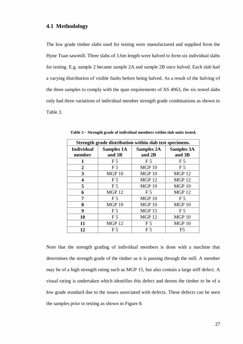
The low grade timber slabs used for testing were manufactured and supplied from the
Hyne Tuan sawmill. Three slabs of 3.6m length were halved to form six individual slabs
for testing. E.g. sample 2 became sample 2A and sample 2B once halved. Each slab had
a varying distribution of visible faults before being halved. As a result of the halving of
the three samples to comply with the span requirements of AS 4063, the six tested slabs
only had three variations of individual member strength grade combinations as shown in
Table 3.
Table 3 – Strength grade of individual members within slab units tested.
Strength grade distribution within slab test specimens.
Individual
member
Samples 1A
and 1B
Samples 2A
and 2B
Samples 3A
and 3B
1 F 5 F 5 F 5
2 F 5 MGP 10 F 5
3 MGP 10 MGP 10 MGP 12
4 F 5 MGP 12 MGP 12
5 F 5 MGP 10 MGP 10
6 MGP 12 F 5 MGP 12
7 F 5 MGP 10 F 5
8 MGP 10 MGP 10 MGP 10
9 F 5 MGP 15 F 5
10 F 5 MGP 12 MGP 10
11 MGP 12 F 5 MGP 10
12 F 5 F 5 F5
Note that the strength grading of individual members is done with a machine that
determines the strength grade of the timber as it is passing through the mill. A member
may be of a high strength rating such as MGP 15, but also contain a large stiff defect. A
visual rating is undertaken which identifies this defect and deems the timber to be of a
low grade standard due to the issues associated with defects. These defects can be seen
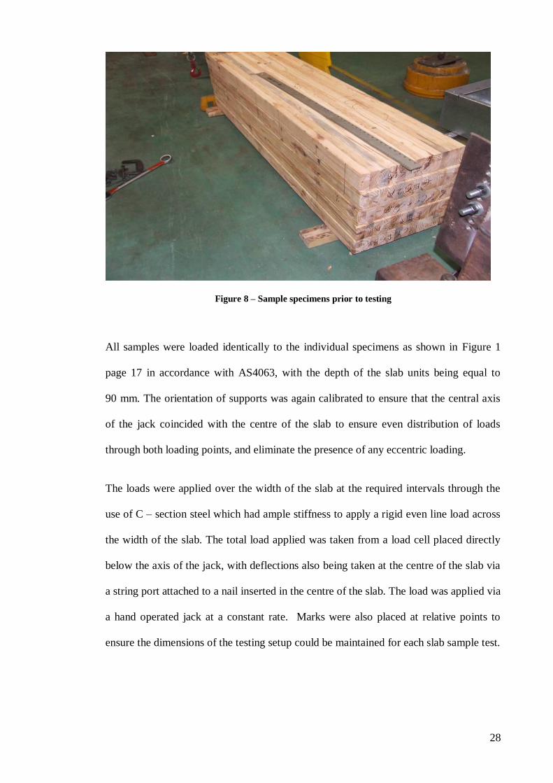
the samples prior to testing as shown in Figure 8.
28
Figure 8 – Sample specimens prior to testing
All samples were loaded identically to the individual specimens as shown in Figure 1
page 17 in accordance with AS4063, with the depth of the slab units being equal to
90 mm. The orientation of supports was again calibrated to ensure that the central axis
of the jack coincided with the centre of the slab to ensure even distribution of loads
through both loading points, and eliminate the presence of any eccentric loading.
The loads were applied over the width of the slab at the required intervals through the
use of C – section steel which had ample stiffness to apply a rigid even line load across
the width of the slab. The total load applied was taken from a load cell placed directly
below the axis of the jack, with deflections also being taken at the centre of the slab via
a string port attached to a nail inserted in the centre of the slab. The load was applied via
a hand operated jack at a constant rate. Marks were also placed at relative points to
ensure the dimensions of the testing setup could be maintained for each slab sample test.

29
Heavy rib reinforced C section steel members were clamped to the stool tops as the
supports for the slabs during loading as shown in Figure 9. The clamps were placed to
eliminate the tendency of the support to roll or slide out form underneath the sample
during loading. Numbers and marks were placed on all relative points of the testing
setup to ensure that the test could be repeated exactly in the future if that was required.
The supporting stools were located on the centreline of the testing rig to ensure that
when the slab was loaded they would not slide or roll out from underneath the sample as
a result of high loads creating resultant forces great enough to displace the stools from
the desired location.
All testing of slabs was undertaken until multiple partial failures had occurred (failure
of individual members within the slab) to get a good description of the patterns of
loading, failure and the new reduced capacity of the slab after one initial failure.
Figure 9 – Slab testing setup.

30
4.2 Results
The Slabs displayed a much more predictable force - deflection characteristic as shown
in Figure 11. It was noted during strength testing that if one half of the slab had on
average a lower grade then the other half of the slab, than the first partial failure would
occur in the weakest half of the slab as shown in Figure 10. The slabs also gave an
indication of the impending failure via creaking noises leading up to a bang which
indicated one partial failure within the slab. The slabs also showed elastic properties.
This became obvious as the load was removed slowly, and the slabs returned to their
original position. It was also noted that a defect within the timber, would fail before the
laminating glue would give way as a result of the induced stresses between members of
different stiffness‟s.
Figure 10 – Low grade slab partial failure.

31
The slabs were consistent within their load – deflection patterns despite the three
variations of member strength grades and the six variations of fault distribution
encountered within the test. The modulus of elasticity determined for each slab unit
tested is shown in Table 4.
Table 4 – Modulus of elasticity of each slab sample
Slab unit number Modulus of elasticity (MPa)
1A 8266.542
1B 8796.801
2A 8653.039
2B 9275.899
3A 9464.317
3B 8776.065
Average 8872.1104
The range of modulus of elasticity values obtained for each slab is very tight compared
to the individual low grade members. The use of individual low grade timber members
to form a laminated low grade slab unit also increases the average modulus of elasticity
compared to the average obtained for the individual members as seen in Table 4.
The small variation in modulus of elasticity values obtained for the two samples
obtained from each combination of individual members demonstrates that the unique
distribution of faults within a low grade slab does have an effect on the structural
performance of low grade timber slabs despite the consistency in the strength grades of
the members used to construct the slab.

32
Figure 11 – Low grade timber slab test results.

33
4.3 Discussion
It can be seen from these results that laminating individual low grade timber lengths
into a slab increase their strength and predictability as structural members due to the
load sharing which arises as a result of the glue laminations. Failure during testing
occurred predominantly on the outside laminates initially with internal laminates failing
afterwards as the slab was reloaded to its new reduced capacity.
This type of failure is proof that the capacity of the low grade timber is increased when
used in slab formation due to the defect free timber sections face laminated adjacent to a
knot which increases the overall resistance to withhold the force applied. An example of
the random distribution of knots and defect free sections within a slab is shown in
Figure 12.
Figure 12 – Random distribution of knots and defect free sections.

34
If these defect free sections of timber were not laminated either side of the faulty piece
of timber it would fail at a much lesser load in a sudden manner due to the absence of
any strong material combined with the defect to increase the overall resistance to
loading induced stresses. This type of failure within a slab would be very similar to that
obtained in the individual low grade member testing due to the effective alignment of
defects as shown in Figure 13.
Figure 13 – Alignment of defects within a slab.
The application of the two line loads across the width of the slab has allowed an
estimation of the range of total load in which the slab is likely to fail; should that value
be applied in total from a combination of uniformly distributed loads and point loads.
Analysis based on Strand7 modelling using the material properties determined during
testing will yield further information in the consistency between the type of load applied
and the deflection and stresses created as a result.

35
4.4 Conclusions
The randomly distributed nature of clean wood and defects within a length of timber
significantly decrease the likely hood of the major defect within a piece of timber being
at the same position along the length of the slab unit in all 12 individual members.
Hence the load sharing between individual members is set up due to the face lamination
acting as an effective strengthening agent for all defects adjacent to clear wood within
the slab.
The distribution of defects randomly throughout the length of the slab results in the slab
having resistance to sudden complete failure due to the load sharing setup between
individual members. The testing confirmed that if one or more members within the slab
failed, the overall load carrying capacity was reduced and the load was taken up by the
adjacent member which had not failed.
Further reliability in strength performance would be obtained if the knots which act as
discontinuities within the timber were located on the compressive edge of the slab, due
to their dense composition which can resist compression but would fail under tension.
This is due to the discontinuity between the grain direction of the knot resulting from
the growth of a branch on the tree and the straight grain of the clear tree trunk.
The load – deflection relationship in slabs is much more predictable than the individual
pieces. The highest load sustained before initial failure of the strongest slab was
107.667 kN. This partially proves that deflection limits are going to be the governing
criteria due to the associated deflection. This will be validated with the use of Strand7
finite element analysis.
Failure of the low grade timber slab units is a function of the location and distribution of
defects throughout each individual member. The slab will not take a bending load

36
greater than that of the strongest individual member if they all contain a knot at the
same position resulting in a sudden line failure as seen in the individual member tests.
The distribution of strength grades within the members of a slab unit can not be used as
a method of determining the exact maximum load the slab can bear. Likewise, the exact
modulus of elasticity associated with any combination of strength grades can not be
determined. This is due to each slab unit having a unique combination of defects which
in turn affect the capacity of the slab. This must be taken into consideration when
designing low grade timber slab floors based on strength and serviceability criteria
through the use of appropriate safety factors.

37
Chapter 5
Finite element analysis
5.0 Introduction
This chapter will focus on the finite element analysis modelling undertaken using
Strand7 to model the performance of low grade timber slab floors. From this modelling,
the limiting criteria for the use of low grade timber slabs as a flooring alternative will be
established. This will be followed by a parametric study to compare the low grade floor
slab characteristics to that of the standard flooring system as shown in Figure 14.

38
Figure 14 – Floor construction configurations
In order to understand the limitations of using low grade slabs as a flooring alternative,
modelling will also be done to develop the deflection relationship between applied load
and clear span. This information is required to create a design chart which defines the
limitations of loading based on prescribed deflection limitations.
Parameters used in this modelling include timber material properties provided by Hyne
and Timber Queensland. Pine density values used in the analysis of the low grade
timber slab floor were based on properties recorded from testing undertaken at the Hyne
Tuan mill as shown in Table 5.
Table 5 – Hyne Tuan mill product densities.
Hyne Tuan mill product densities (kg/m³) (untreated) 140x35 Dry 70 x 35 Dry 90 x 35 Dry 70 x 45 Dry 90 x 45 Dry Average
Utility* 590 617 604
F5 557 553 552 554
M10 564 576 568 555 557 564
M12 609 625 617 596 607 611
M15 661 685 665 670
* Utility is the term used by Hyne to describe its low grade timber product.

39
5.1 Selection and justification of appropriate modelling parameters.
An analysis on the three major types of element which the slabs could be modelled with
was performed in order to establish which type gave the most accurate depiction of the
behaviour of the slab samples observed during testing. All models were made to
represent slab sample 2A with a modulus of elasticity of 8653.0386 MPa. The load and
deflection summary for this sample are shown in Table 6 . All three of the models were
assigned the same material properties and supported as simple beams. Analysis of each
model was then done to how well they replicate the physical test data.
Table 6 – Load - deflection summary for sample 2A
Slab 2A recorded test data
Load (kN) Deflection (mm)
0 0
20 7.6
40 14.5
60 21.0
80 28.2
100 37.6
The following three sections will go through and make a comparison between each of
the model dimensions to justify the reasoning in the model type chosen. All models
have been created with consistency in material properties, load application and restraint
type in order to justify the comparison between results.
40
5.1.1 One dimensional beam element model
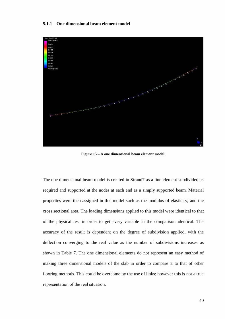
Figure 15 – A one dimensional beam element model.
The one dimensional beam model is created in Strand7 as a line element subdivided as
required and supported at the nodes at each end as a simply supported beam. Material
properties were then assigned in this model such as the modulus of elasticity, and the
cross sectional area. The loading dimensions applied to this model were identical to that
of the physical test in order to get every variable in the comparison identical. The
accuracy of the result is dependent on the degree of subdivision applied, with the
deflection converging to the real value as the number of subdivisions increases as
shown in Table 7. The one dimensional elements do not represent an easy method of
making three dimensional models of the slab in order to compare it to that of other
flooring methods. This could be overcome by the use of links; however this is not a true
representation of the real situation.

41
Table 7 – One dimensional Strand7 model convergence and comparison.
One dimensional element model convergence
Number of Beam
elements
Deflection obtained from model (mm)
20 kN
Load
40 kN
Load
60 kN
Load
80 kN
Load
100 kN
Load
3 6.8 13.6 20.4 27.2 34
6 6.8 13.7 20.5 27.3 34.2
12 6.8 13.7 20.5 27.3 34.2
Physical test values 7.6 14.5 21.0 28.2 37.6
Difference to
physical test values 0.8 0.8 0.5 0.9 3.4
This demonstrates that the minimum number of beam elements in a one dimensional
model has to be greater than or equal to 6 over a 1.62 m span for convergence to occur.
The difference observed in Figure 16 at loads greater than 80 kN is due to the fact that
the slabs do not load and deflect in a perfectly linear fashion as seen in Figure 11. This
means the model is only representative for the linear load – deflection range of the slab.
Figure 16 – Comparison between one dimensional model and physical results.

42
5.1.2 Two dimensional plate element model
Figure 17 – A two dimensional plate element model.
The use of two dimensional plate elements to represent the beam resulted in identical
results to that of the one dimensional element for each number of subdivisions. The
plate was assigned a thickness of 90 mm and subdivided 24 times in the X direction, 18
times in the Y direction, with the Z direction containing only 1 element due to the two
dimensional nature of the model resulting in a total of 432 plate elements. This number
of plates in the model resulted in deflection values which matched the converged one
dimensional model for each load case applied.
The application of the two dimensional model to three dimensional comparative
models is not appropriate due to the issues associated with combining nodes in the
correct relative positions. This issue arises due to the nodes being at the middle of the
slab, hence the neutral axis is fixed to the supporting element rather than the tension
edge. This will yield the correct relationship between the slab and the supporting

43
element under the influence of loading. The use of links to create a three dimensional
model using two dimensional elements would be sufficient to obtain correctness in the
dimensions of each element and their location relative to each other. However, the issue
of incorrect stresses being transferred from the slab to the supporting joist are still
present due to the link being made at the neutral axis rather than the tensile face of the
slab.
Minor issues also arise from the loading of the slab at the central axis rather than the top
edge in the two dimensional models. The central location of the plane of nodes in the
two dimensional slab models is shown in Figure 18.
Figure 18 – Node location within a two dimensional slab model cross section
The two dimensional model lacks accuracy in the prediction of bending stresses on the
tensile face of the slab. This is due to the single elements in the vertical direction which
have a single stress assigned to them during analysis rather than a distribution of
stresses throughout the depth of the slab as occurs in the slab during loading and
modelling using three dimensional brick elements. The analysis of the slab as a flooring
material needs accuracy in the modelling of working stresses to ensure that allowable
stresses are not exceeded.

44
5.1.3 Three dimensional brick element model
Figure 19 – A three dimensional brick element model.
The use of three dimensional modelling elements yields slightly different results to that
of the two dimensional elements and one dimensional element models. It was found that
a high number of bricks could be used efficiently for both convergence in results and
accuracy in stress distributions created as a result of various load patterns being placed
on the slab. A comparison between the three model types is shown in Table 8 to portray
the difference in results obtained from each model type.
Table 8 – Strand7 model comparison
Model
type
Number
of
elements
Deflection obtained from model (mm)
20 kN
Load
40 kN
Load
60 kN
Load
80 kN
Load
100 kN
Load
1D Beam 12 6.8 13.7 20.5 27.3 34.2
2D Plate 432 6.8 13.7 20.5 27.3 34.2
3D Brick 6480 6.87 13.75 20.62 27.5 34.37
Physical
Model 1 7.6 14.5 21.0 28.2 37.6

45
Modelling with three dimensional elements also results in a more accurate description
of the distribution of stresses within the slab as a result of loading. This is crucial for the
accurate modelling of the slabs to predict the load and span relationship which results in
the allowable stress levels within the slab being exceeded.
The use of three dimensional brick elements in modelling is also preferable for the
creation of three dimensional models of flooring systems. This is due to the ease at
which members can be connected in a way which accurately represents the connection
in the physical model, and the capability to assign unique material properties to
individual brick elements as appropriate due to the arrangement of nodes as shown in
Figure 20.
Figure 20 – Node location within a three dimensional slab model cross section.
5.1.4 Use of isotropic elements
Orthotropic elements should be used to model timber; however sufficient material
information for timber in the three required directions is not available for low grade
slabs due to no prior work being done in this area. The properties of pine alone could be
used but this option was not taken due to the differences induced as a result of the glue
laminations between pine members of varying strength grades.

46
Therefore the slabs were modelled as three dimensional isotropic elements due to the
highest level of accuracy which was returned in the results compared to the physical test
results. The modulus of elasticity used in this model was calculated using Matlab to
determine the linear proportion of the load – deflection curve and calculate the modulus
of elasticity based on this interpretation. This is the reason for the slight difference in
the modelled slab deflection and the physical test deflection as seen in Figure 21. Note
that all differences in deflection on the linear region of the graph are less than one
millimetre, with the major differences between the modelled performance and the
physical performance being at higher loads. This occurs where the load – deflection
relationship is not linear as can be seen at the 100 kN load data points for each model in
Figure 21.
Figure 21 – Comparison of Strand7 models to physical test results.

47
5.1.5 Application and justification of chosen poisons ratio
The poisons ratio for all Strand7 models had to be chosen and validated due to no
existing data on the poisons ratio values for low grade timber slabs. This is due to no
prior investigation into the effects that glue laminations have on the poisons ratio of low
grade pine.
The investigation was based around using the established three dimensional brick
element model with various values of poisons ratio to determine the extents of the error
within the model and design aids as a result of using a poisons ratio value which does
not represent a proven value.
As the three dimensional brick elements are modelled as isotropic, one poisons ratio
value was applied in all three axis. This is not a true replication of timber due to its
unique properties in each of the three axis. Despite this, the results comparison between
the three dimensional brick element model and the physical results prove that using a
unique poisons ratio in all three directions is sufficiently accurate.
The result of varying the poisons ratio is shown in Table 9. It can be seen that there is a
slight increase in the deflection value obtained from the model as the value used for
poisons ratio increases. Therefore the poisons ratio value of 0.2 was chosen as the
optimal value to ensure that the model results are as close to the physical test results as
possible as seen in Figure 22, and design aids based on Strand7 models are an over
estimate of the slabs characteristics as a slight factor of safety incorporated into the
design charts.

48
Table 9 – Difference in model outputs for various poisons ratio values.
Load Case
Deflection recorded for a slab
span of 6.0 m with varying
values of poisons ratio (ν) (mm)
Maximum difference
in deflection for given
poisons ratio values ν = 0 ν = 0.1 ν = 0.2
Self Weight 15.7 15.8 15.8 .1
1 kN/m² 29.1 29.3 29.4 .3
Self weight + 1 kN/m² 44.8 45.1 45.2 .4
Self weight + 2 kN/m² 73.8 74.4 74.5 .7
Self weight + 3 kN/m² 102.9 103.7 103.9 1
Self weight + 4 kN/m² 132.0 133 133.2 1.2
Self weight + 5 kN/m² 161.1 162.3 162.6 1.5
Self weight + 7.5 kN/m² 233.8 235.6 236.0 2.2

49
5.2 Methodology
The Strand7 modelling is intended to allow an accurate prediction of the low grade
slabs response to loadings typically endured by floor structures. Its secondary function
is to draw comparisons between the structural performances of the typical floor
consisting of bearer‟s, joists and flooring material, and that of the low grade slab
flooring system which consists only of bearers and the slab. The Strand7 finite element
analysis was used to analyse the slabs based on the following two floor design criteria:
Deflection based assessment.
Maximum limiting stress based assessment.
The limiting stress has been determined using the stress distribution in a simple beam
and the lowest load applied to cause the first partial failure within the slabs. The lowest
load to cause a partial failure was taken from the test data as 75000 N. This load is
transferred to its equivalent bending moment via the bending moment diagram shown in
Figure 22.
Figure 22 – Derivation of maximum moment from loading setup.
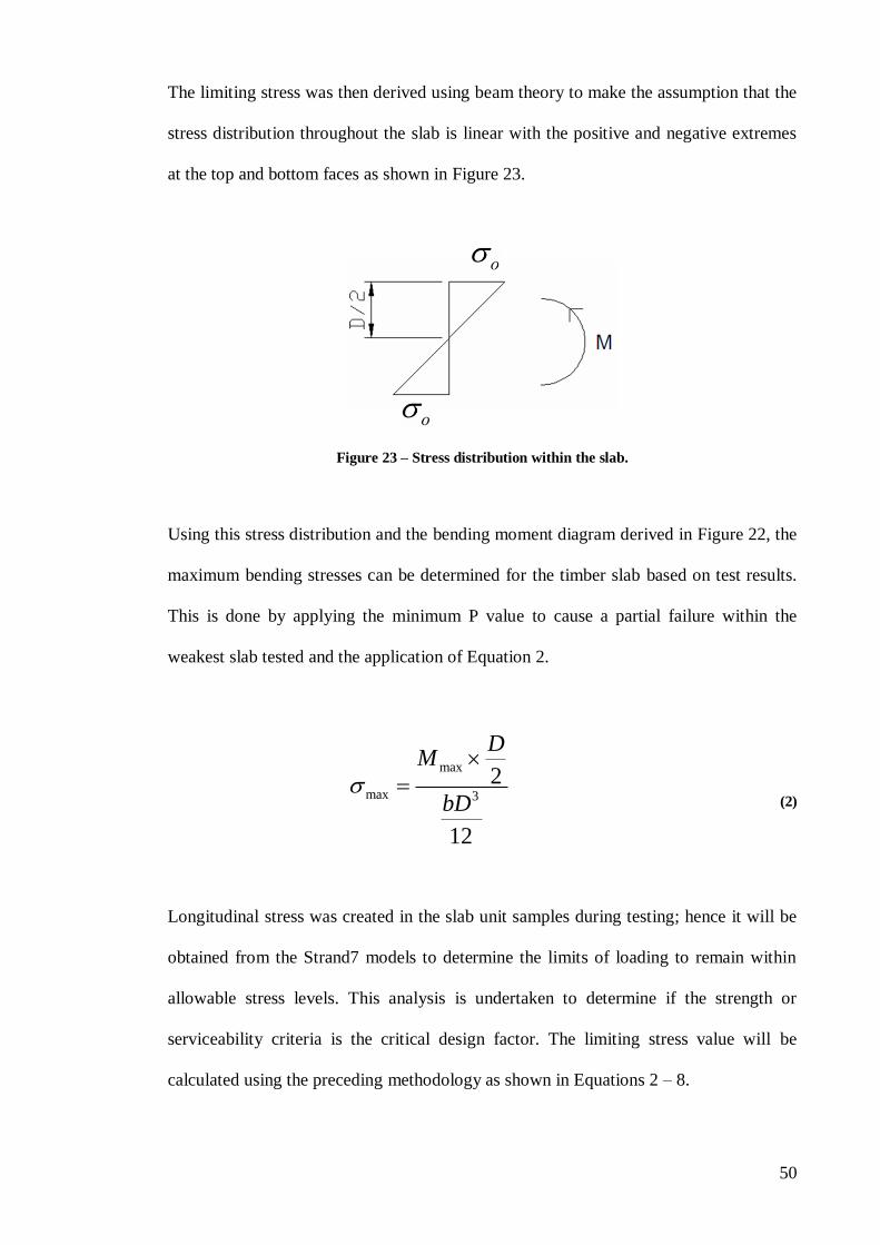
50
The limiting stress was then derived using beam theory to make the assumption that the
stress distribution throughout the slab is linear with the positive and negative extremes
at the top and bottom faces as shown in Figure 23.
Figure 23 – Stress distribution within the slab.
Using this stress distribution and the bending moment diagram derived in Figure 22, the
maximum bending stresses can be determined for the timber slab based on test results.
This is done by applying the minimum P value to cause a partial failure within the
weakest slab tested and the application of Equation 2.
max
max 3
2
12
DM
bD
(2)
Longitudinal stress was created in the slab unit samples during testing; hence it will be
obtained from the Strand7 models to determine the limits of loading to remain within
allowable stress levels. This analysis is undertaken to determine if the strength or
serviceability criteria is the critical design factor. The limiting stress value will be
calculated using the preceding methodology as shown in Equations 2 – 8.

51
75 P kN (3)
.09 D m (4)
18 18 .090 1.620 L D D m (5)
max
75 1.6220.25 .
6 6
PLM kN m
(6)
3 35 4.420 .09
2.25515 1012 12
bDI m (7)
max
max 5
.0920.25
2 2 35,714 / ² 35.714 2.25515 10
DM
kN m MPaI
(8)
Based on these calculations the limiting longitudinal stress value is 35.714 MPa. This
value will be used with the low grade slab model to determine the maximum load that
may be applied to a floor slab consisting of numerous connected individual slab units.
The same models will also be used to measure the floor slab deflection for the same
load distribution with a varying range of intensities from the slabs response to self
weight up to self weight plus 7.5 kN/m² of force over a slab of 3.6 m width and spans
varying from 1.8m in multiples of 600 mm through to 6.0 m. The standard floor
construction model will be used in the same way with the limiting stress in the
hardwood joists taken as 80 MPa for F27 grade timber from AS1720.1 – 2002.
The results obtained from this analysis will define stress or deflection as the limiting
criteria based on which is exceeded first as a result of increased loading on the floor
slab.

52
5.2.1 Parametric study between slab and standard flooring
The parametric study between the low grade timber slab construction system and the
standard bearer, joist and flooring material construction method was done in order to
determine the differences in responses when loads of various magnitudes were applied
to both models.
Both construction methods were modelled with identical bearers, with the difference
being the slab model had only the low grade slab on the bearer, and the standard model
had joists and flooring of the same material as the bearer. This was done so that the
models could be compared with as few variables as possible, as any difference in
material or dimensions of the bearer would yield a result of no comparative value.
The standard floor models and the slab floor models were created with a width of 3.6 m
and varying floor spans for consistency between models. The load was uniformly
distributed by calculating the load of 1 kN/m² over the area of the slab divided by the
number of nodes in that floor area. The resulting load was then applied to each node
within that area. For example the floor model 3.6 m wide and 4.8 m in span with 7408
nodes, had a total load applied to each node as shown in Equation 9. A complete list of
models and applied loads used in the parametric study is given in Table 10.
1 3.6 4.8 17.28
.0023326134 /Number of nodes 7408
kN m m kNkN node
(9)

53
Table 10 – Model dimensions used in study with 1 kN/m² node loading values.
Model dimension
(Width x Span) Model type
Applied load
(1 kN/m²)
Number of
nodes
Load / node
(kN)
3.6 m x 3.6 m slab
12.96 kN 22,630 .00057
standard 5,620 .00230
3.6 m x 4.2 m slab
15.12 kN 26,275 .00057
standard 6514 .00232
3.6 m x 4.8 m slab
17.28 kN 29,920 .00057
standard 7,408 .00233
3.6 m x 5.4 m slab
19.44 kN 33,565 .00057
standard 8,302 .00234
3.6 m x 6.0 m slab
21.60 kN 37,210 .00058
standard 9,196 .00234
The various load magnitudes were applied to the model by creating the following two
load cases within Strand7 and then combining them and multiplying by the appropriate
factor to achieve the required total load:
Self weight (gravity)
1 kN/m²
This results in linear load case combinations, which are applied to the floor model
allowing the predicted deflections and stresses to be recorded. Each model was run
initially to record the stress in supporting members and the deflection of the floor as
shown in Figure 24.

54
Figure 24 – Standard floor construction Strand7 model
Each model used in the parametric study was simply supported on each of the four
corner nodes to allow translation in the two dimensional floor planes without allowing
any vertical movement within the model as shown in Figure 25. This is realistic for a
floor area supported by free standing columns as the columns will deflect inwards as a
result of loads being applied to the flooring area. This restraint system has been chosen
due to maximum level of deflection which will occur at the centre of the supported floor
area. Restricting translation in the Z - X plane would result in tension being developed
in the supporting members. The resulting deflection maximum deflections would
therefore be reduced.
For the bearer in the standard and slab model, the joist in the standard model and the
slab in the slab model to be simply supported, no other method of restraint can be used.
This is due to the fully fixed nature of the connection between the joists / slab to the
bearer in the standard and slab models respectively. The slab model was made with a

55
full connection between the edge of the bearer and the floor slab for the entire width of
the model as shown in Figure 26.
Figure 25 – Supports used in Strand7 floor models
Figure 26 – Low grade timber slab floor Strand7 model

56
The material properties used in both models were derived from data obtained through
testing, Hyne quality assurance data and spreadsheets containing hardwood tests
undertaken by Timber Queensland. The material data used in each model can be seen in
Table 11.
The standard floor model used in the parametric study consists of a bearer, joists and
flooring material as shown in Figure 24. The low grade slab model consists of an
identical bearer but the flooring material and joists are replaced by the low grade slab as
shown in Figure 26.
Table 11 – Material dimensions and properties used in Strand7 models.
Member Length
(mm)
Width
(mm)
Depth
(mm) Material
Modulus of
Elasticity
(MPa)
Density
(kg/m³)
Poisons
Ratio
Bearer 3600 50 200 Grey
Ironbark 18702.65 1097.665 0.2
Joist span 50 100 Grey
Ironbark 18702.65 1097.665 0.2
Floor span 3600 19 Grey
Ironbark 18702.65 1097.665 0.2
Slab span 3600 90
Low
grade
pine
8872.11 604 0.2
Note that length in this table implies the span referred to in table 10 plus 100mm
for the member to cover the clear span plus the width of the supporting bearers.

57
5.2.2 Modelling of slab performance to create design chart
To demonstrate the performance of the low grade slabs, their structural performance
was modelled with Strand7 over eight spans and six separate load cases. To ensure that
the chart was representative of the slab behaviour only, the bearer was removed to
eliminate the deflection it adds to the system, and the associated two way bending
effects. The model was simply supported at its four corners and fully supported against
deflection in the vertical direction in the place of the bearers to ensure that only one way
bending could occur within the model. This was done to represent a realistic support,
loading and deflection situation.
Each model was made 3.605 m wide, due to the width of the members in each slab unit
of 35 mm which makes it impossible to create a slab of complete individual members
3.6 m wide exactly. The slab density was taken as 604 kg/m³ as this is the average value
recorded for the low grade product produced by the Hyne Tuan mill. The following
models were run to create the design chart with the loads applied for each response by
the model as shown in Table 12.
Table 12 – Total load applied for each load case in Strand7 models.
Clear
span
(m)
Total load applied for each load case (kN).
Self
Weight
1
kN/m²
Self
Weight + 1
kN/m²
Self
Weight + 2
kN/m²
Self
Weight + 3
kN/m²
Self
Weight + 4
kN/m²
Self
Weight + 5
kN/m²
1.8 3.46 6.489 9.949 16.438 22.927 29.416 35.905
2.4 4.61 8.652 13.266 21.918 30.570 39.222 47.874
3.0 5.77 10.815 16.582 27.397 38.212 49.027 59.842
3.6 6.92 12.978 19.899 32.877 45.855 58.833 71.811
4.2 8.07 15.14 23.215 38.356 53.497 68.638 83.779
4.8 9.23 17.304 26.532 43.836 61.140 78.444 95.748
5.4 10.381 19.467 29.848 49.315 68.782 88.249 107.716
6.0 11.535 21.630 33.165 54.795 76.425 98.055 119.685

58
These loads were applied to the slab model by having Strand7 calculate the self weight
load created by a gravitational force of -9.81 m/s/s as one separate Load case. The
Uniformly Distributed Loads (UDL) were applied as a separate load case to the nodes
joining brick elements that make up the slab by dividing the total force created by
1 kN/m² over the slab area by the number of nodes on the top surface of the slab as
shown previously in Equation 9.
The load combination cases were applied to the model by creating load cases within
Strand7 which take the self weight and combine it to the 1 kN/m² UDL multiplied by
the appropriate factor to create a load case of the desired magnitude as shown in Figure
27. 1 kN/m² was used as the base value for the ease of load case creation associated
with a unit value.
Figure 27 – Strand7 load case combination screen print.
Each model was than run to analyse the deflection caused by the applied load over the
given span and width, with the vertical deflection in the centre of the slab recorded.
Once the load deflection lines were plotted, further lines were created to join the distinct
load case results on each span. Deflection limit lines were also superimposed on the
load deflection curves for each span. These lines are curved due to the variation of
limiting deflection value with change in span for a set deflection limit ratio. This was
done to allow interpolation of values when used in a design situation. For example
taking a required load and deflection limit and using those values to solve for the
maximum clear span which can be used with a low grade timber floor slab.

59
5.3 Results
Using a deflection limit of span / 250 the loads required to exceed the limit on each
model type are shown in Table 13. This comparison yields results based on the average
linear section of the load / deflection graphs obtained during the testing of the slabs, and
hardwood material data obtained from Timber Queensland and AS1720.1 – 2002. The
relationship between stress and deflection limits based on applied load is shown in
Figures 28 – 21.
Table 13 – Stress and deflection limit comparison
Model Deflection
limit (mm)
Deflection
based load
limit (kN)
Stress
limit #
(MPa)
Stress
based load
limit (kN)
Equivalent
deflection *
(mm)
3.6m x 3.6m
slab 14.4 42.628 35.714 373.043 126
3.6m x 3.6m
standard 14.4 27.375 80 167.612 88
6.0m x 3.6m
slab 24 18.068 35.714 253.993 337
6.0m x 3.6m
standard 24 14.851 80 123.887 198
* Proportional linear deflection caused by the load required to meet the stress limit.
# Hardwood bending stress limit obtained from AS1720.1 for F27 grade timber.
Based on this modelling, the span limitations required for the stress and deflection limit
to be obtained from the same load are as follows:
3.6 m x 3.6 m slab – Span / 28.57
3.6 m x 3.6 m standard – Span / 40.91
6.0 m x 3.6 m slab – Span / 17.80
6.0 m x 3.6 m standard – Span / 30.18

60
Figure 28 – 3.6m span deflection limit graph for both floor model types.
Figure 29 – 3.6m span stress limit graph for both floor model types

61
Figure 30 – 6m span deflection limit graph for both floor types
Figure 31 – 6m span stress limit graph for both floor types

62
5.2.3 Parametric study between slab and standard flooring
The comparison between the low grade slab floor system and the standard system yields
results that show that the slab floor construction method can take a greater load than the
standard method with a deflection that is significantly less as shown in the following
graph. The reason for the larger total load is the self weight of the low grade slab due to
the bulk of low grade timber used, compared to the skeleton structure of the standard
method of floor construction.
Figure 32 – Comparison between a standard and a low grade timber slab floor.
The calculation of the self weight included in the total load shows that the relationship
between span and total load applied for each load case is not linear as assumed prior to
modelling and analysis. It can also be seen that the deflection increases as a result of
each load case within the standard model are significantly greater than that of the slab
model.

63
5.2.4 Low grade timber slab design chart
The analysis of the low grade slab without any supporting bearer returned the deflection
results shown in Table 14. This information is used with the total load information
provided in Table 12 to plot the load deflection curves for slabs having a clear span
range of 1.8 m – 6 m as shown in Figure 33. All deflections recorded are the maximum
value obtained from the centre of the slab. Due to the deflection limits being the
governing criteria no evaluation was done on the variation of stress levels within the
slab as the load increases.
Table 14 – Low grade slab deflections for each load case.
Clear
span
(m)
Maximum deflection for each load case (mm).
Self
Weight
1
kN/m²
Self Weight
+ 1 kN/m²
Self Weight
+ 2 kN/m²
Self Weight
+ 3 kN/m²
Self Weight
+ 4 kN/m²
Self Weight
+ 5 kN/m²
1.8 0.4 0.3 0.7 0.9 1.2 1.5 1.7
2.4 0.5 0.8 1.3 2.1 2.9 3.8 4.6
3.0 1.1 2 3.1 5.1 7.2 9.2 11.2
3.6 2.3 4.2 6.4 10.6 14.8 19 23.2
4.2 4.2 7.7 11.9 19.6 27.3 35 42.8
4.8 7.1 13 20.1 33.1 46 59 72
5.4 11.3 21 32.2 53.2 74.2 95.1 116.1
6.0 17.1 31.9 49 80.9 112.7 144.6 176.4

64
APPLICABLE TO A SLAB DEPTH OF 90 MM ONLY
Figure 33 – Low grade timber slab design chart.

65
5.3 Discussion
The limiting design criteria analysis undertaken on the low grade slab demonstrates that
the structural capacity of the slab is limited by the deflections induced as a result of
loading. The limiting stress value applied to the low grade slabs was determined from
the lowest load required to cause a partial failure in the six individual slab units tested.
Further testing of a larger sample may yield that the stress value used here is not the
lowest stress which will result in a partial failure of the slab, hence further testing of the
slabs should be carried out, and a factor of safety used in all calculations. The analysis
of the models is linear whereas the physical test results obtained from the testing of low
grade slab units is only linear in the lower load regions as can be seen in Figure 11.
Therefore the values are not accurate over all portions of the load – deflection graph, but
descriptive of the relationship between applied load and corresponding deflection. This
can not be avoided in the linear analysis due the average modulus of elasticity used.
This value was derived from the linear portion of the data obtained from the testing of
individual low grade slab units.
It should also be noted that the maximum stress has been derived based on a four point
loading setup which is not likely to occur in a typical floor loading situation. Therefore
further testing should be undertaken which incorporates a series of point loads and
uniformly distributed loads to obtain a stress limit that is the resultant of a realistic floor
loading situation.
The analysis also demonstrated that the stress limit is reached in the standard floor
structure at a significantly lower load than that of the slab structure. This result is valid
due to the identical bearer used between the two models, and the skeleton structure of

66
the standard construction method, which has a significantly less volume of timber
resisting applied forces.
5.3.1 Parametric study between slab and standard flooring.
The parametric study between slab and standard flooring analysed the effects of
different load magnitudes based on models of identical dimensions. The bearer used in
both model types to support the joists and the low grade timber slab was identical. This
was done to eliminate one variable in to make results comparable. In reality these
bearers could be manipulated to make the deflection comparison between the model
types identical.
The slab model is effectively a standard model with no spacing between the joists, and
no presence of flooring material. Therefore the weight of the structure is significantly
greater than that of the standard method of construction. It also results in a larger
resistance to applied load which is evident in the results obtained from modelling. The
larger load is partly due to the greater self weight of the structure, but the results from
both models contain identical applied loads. Therefore the comparison yields that the
low grade timber slab construction system can take a larger load before exceeding
deflection limits than the standard method of floor construction.

67
5.3.2 Low grade timber slab design chart.
The low grade timber slab design chart was created using average values for the
modulus of elasticity and the density of low grade pine. The density value used is the
average value from a large number of tests and is therefore a representative value. The
average modulus of elasticity used is the average of six tests only. The tests proved that
the variance in modulus of elasticity is not large; however further testing would reveal
trends which can be used to refine the model. For this reason an appropriate factor of
safety should be included if using the base representative values shown in the design
chart.
The modelling carried out to develop the design chart was linear. This does not
represent the true load deflection characteristic of the slab; however it is a close
approximation to the average deflection that can be expected for an applied load. The
modelling has also been done based on the 90 mm deep slab units tested, width of
3.605 m which represents 103 individual low grade timber members within the slab.
This value was used due to each individual member within the slab being 35 mm wide
and the need for comparability with the standard 3.6 m wide floor used in the parametric
study.
Equation 10 represents the deflection of a simply supported beam, subjected to a
uniformly distributed load which can be used to describe the behaviour of the slab in
one way bending.
45
384
wL
EI (10)
This can be used to justify that as the span increases and the same uniformly distributed
load is applied, the increase in load as a function of floor area, and the increase in

68
rigidity of the slab as result of the extra width have no effect on the total deflection at
the centre of the slab.
Using Equation 10 to validate the low grade slab design chart for a load of 1 kN/m² and
a clear span of 4.8 m, the deflection obtained is as shown in Equation 11. The results
obtained from the linear Strand7 finite element analysis model indicate that the resultant
deflection is 13mm as can be seen in Table 14.
4
3
1 3.605 4.8512.82
384 3.605 .098872.11
12
mm
(11)
Applying this equation for a slab of 20 m width, it can be seen via Equation 12 that the
difference in central deflection is the same; therefore the design chart can be used for
any required span subjected to a uniformly distributed load with accuracy.
4
3
1 20 4.8512.82
384 20 .098872.11
12
mm
(12)
The difference in deflection between theoretical values and the value obtained from this
particular model are .18 mm different. This is most likely due to the effect of the
poisons ratio value of 0.2 used in all models. Convergence within the finite element
analysis model is present and therefore the model values represent the best
approximation to the deflection based on the material specific properties used in the
model.

69
5.4 Conclusions
Comparative models of the standard and the slab flooring system have shown that the
low grade timber floor slabs can perform better than the standard floor, as equivalent
loading on top of the self weight causes a considerably greater deflection in the standard
floor than it does in the slab. The slab has proven to perform better than the standard
floor construction method in both stress and deflection based analyses.
The results are reliant on a lot of variables which could be manipulated to make the
standard flooring method perform better than the slab, however this would only happen
if the joists were spaced more closely than that of standard practice. If a model were
created like this the results would be effectively converging on that of the slab floor, i.e.
joists with zero spacing on a bearer are the same as a slab.
The isotropic brick elements used to model the flooring systems has been proven to be
adequate despite the single direction modulus of elasticity and poisons ratio value that
do not accurately depict the real structure. Tests models were run between Strand7 and
the standard single slab units with results within 0.5 mm of the recorded deflections.
Theoretical results also yield a value which is within 0.5 mm of the model.
The low grade slab design chart accurately describes the structural limitations of using
low grade timber as a one way floor slab based on the six sample slabs tested. This
development provides a reasonably safe method of designing a floor that is required to
exceed the capacity of the standard method of floor construction over set spans.
The design of appropriate bearers to support the weight of the slab and the applied load
shown in the design chart can also be undertaken based on the total load values
presented. This implies that two way bending will be present within the slab if the
deflection within the supporting bearer is significant. Further research into the

70
performance of slabs subjected to two way bending is required to determine the exact
capabilities of a low grade timber floor slab in this situation.
The elimination of the extra floor depth associated with the joists required to support
flooring material in standard floor construction is a major advantage of using low grade
slabs for above ground flooring applications. The extra head room created allows better
use of space for installation of essential services without compromising structural
integrity or ceiling height.
71
Chapter 6
Connections
6.0 Introduction
This section is aimed at developing connection methods and investigating the
performance of connections between low grade timber slab units acting as a floor slab.
Research of this nature has not been undertaken previously due to the fact that this is the
first work which investigates the effectiveness of using low grade slab units as a
flooring alternative. The development of a suitable connection method involves the
development of multiple conceptual prototypes, with the process of elimination based
on required characteristics.

72
The major force that will be present in the joint is a shear force due to the differential
deflection that occurs as a result of differences in the stiffness of each individual slab
unit, and separation of slab units that could occur if the slab is subjected to a tensile
force perpendicular to the direction of the laminates.
The aim of the connection strength in all directions is to exceed that of the strength of
the glue that is laminating the timber pieces together into a slab, and also exceed the
strength of the timber itself when subjected to any force which the connection is
expected to withstand.
This presents a challenge as the strength of individual members in bending, shear and
tension has been proven to be highly variable. Therefore the analysis has to be done
based on the expected load range that will be applied to the slab which will not cause
deflections greater than the given design maximums.
Moisture related effects on joint performance have been taken into consideration,
however a full analysis of the effects of moisture on low grade timber floor slabs is
outside the scope of this research work. This needs to be given a more detailed analysis
in future research work related to the appropriateness of low grade timber slab units
used in floor construction.

73
6.1 Methodology
Initial investigation on slab unit connection required a determination of the most
appropriate connection method. To do this, a range of ideas were established and
weighted to show the most appropriate one in terms of:
Connection suitability to resist shear - A
Connection suitability to resist tension perpendicular to the laminates - B
Ease of manufacture and construction - C
Envisaged cost of materials + manufacture + transport + construction - D
Time taken to manufacture, transport and construct - E
6.1.1 Connection methods evaluation
Multiple ideas were created, and investigated on their merit in the factors listed in
section 6.1. Many methods of forming a connection to resist a single force were thought
of, however only those that could meet the two criteria in some capacity were used for
further analysis to pick the most suitable prototype to construct and test. The selected
ideas included:-
IDEA 1 - A single high grade timber plank jointed into the face of the
connecting slabs
IDEA 2 - A plank spanning the length of the slab with nails or screws driven
directly into each member.
IDEA 3 - A large dovetail block fixed into a pre-cut joint in the slabs
IDEA 4 – 140 mm deep laminates on the outside edges of each slab with bolts
connecting them together underneath the slab.

74
IDEA 5 - Bugle Head batten screws skewed into the slabs and counter sunk
below the surface.
Reference: See Appendix F for diagrams of each of these ideas.
6.1.2 Selection using weighted decision matrix
The conceptual connection ideas were evaluated to determine which best met all of the
requirements of a slab unit connection. This was done using a weighted decision matrix
as shown in Table 15. Each of the ideas was compared with each of the criteria which
have to be met by a connection in order to be practical and effective. Numbers were
used as the weighting factor with five representing an excellent fit to the criteria, and
one representing a very poor fit to the criteria. The score of each idea was than
determined by summing each of the criteria ratings for each idea to get a total score for
each idea.
From this evaluation it can be seen that the bugle head batten screw concept made an
excellent fit to all required criteria, followed by the spanning plank concept which did
not fit all the criteria to the same extent. Based on this decision making, the bugle head
batten screw concept been perused.
Table 15 – Connection method evaluation matrix
IDEA
Criteria Rating
A B C D E Total
1 1 1 5 4 3 9
2 3 5 5 3 3 19
3 2 3 1 1 2 9
4 4 3 1 2 2 12
5 5 5 5 5 5 25

75
6.1.3 Bugle head batten screw testing methodology
The aim of the connections investigation is to establish a method of joining two
adjacent slabs that is stronger than the glue itself, and the low grade timber.
The method of constructing the joint involved marking the centre of the second laminate
in from the edge of the slab unit and drilling a countersinking hole so that the heads of
the screws were just below the surface of the slab, and would penetrate to the depth
shown in Figure 34 .
Figure 34 – Cross section of chosen connection method
A 4 mm pilot hole was then drilled at 30 degrees to the horizontal into the slab to guide
the screws in at the correct angle. The pilot hole did not extend through the edge of the
slab unit. The two main purposes of this starter hole were to ensure the correct angle
was achieved and a looser level of friction was present in the slab which the screw was
being driven from to ensure that all screws pulled the slabs together to their greatest
capacity. After the pilot holes had been created, 125 mm bugle head batten screws were
driven into the holes and through into the adjacent slab as shown in Figure 35. Bench
clamps were applied over the span of the slab to ensure that the screws pulled tight and
formed a bond between the slabs equal to the screws capacity.

76
Figure 35 – Arrangement of bugle head batten screws.
The method used to ensure that all screws entered at the correct angle was to cut a waste
piece of pine at 30 degrees, and use this surface to run the drill into the countersinking
hole at the set angle as shown in Figure 36. This initial hole angle was then used as a
guide to complete the clearance hole which only ran from the starting slab to the
interface between slab units. This helped to ensure that the screws embedded in the
adjacent slab unit to their maximum capacity.

77
Figure 36 – Creating the correct angle for the screw joint.
Screws were driven into at 200 mm centres from both sides of the joint into the
opposing slab. The joint lines were staggered so that one screw was passing into the
opposing slab at every 100 mm throughout the length of the slab as shown in Figure 37.
Figure 37 – Plan view of chosen connection system

78
6.1.3.1 Two slab bending test
To do this the initial test was two slabs joined together with 14G 125 mm bugle head
batten screws skewed into the slabs at 200 mm centres from both slabs into the adjacent
slab as shown in Figure 37.
Once the slabs were connected, they were arranged under the testing rig to meet the
dimensions of testing as used in previous individual sample and slab tests. Heavy duty
“I” beams and Square sections were used to get the required heights and spans so that
the appropriate loading support conditions were met. Figure 38 depicts the testing setup
applied.
The system 5000 was then connected with two string ports and a load cell, to measure
the applied load, and the deflections of the slab being loaded, and the slab which was
connected to the loaded slab with no load applied, to obtain a measurement in the
difference in deflection, or deflection passed through the connection as load was
applied.
Figure 38 – Loading setup for two slab bending test.

79
6.1.3.2 Three slab shear and bending test
The three slab connection test consisted of three individual slab units joined at the edges
using the connection method shown in Figure 34 and Figure 37. In order to apply the
loads at the required intervals over the width of one slab, heavy duty solid steel sections
were cut to 420 mm lengths to apply a line load over the width of the centre slab only.
A heavy duty steel section was used to ensure that zero deflection occurred within the
line load bar resulting in an even distribution of applied force across the distribution of
the slab.
The supports were setup to provide a vertical restraint at the ends of the outside slabs
only, with the centre slab being free to push down through between the other two if a
shear failure happened before the bending failure. To do this heavy C sections were
placed on a long supporting beam so that the inside ends of the heavy C sections were
supporting the laminate on the outside slabs that is adjacent to the centre slab. This was
done to initiate a shear failure along the connection between the centre slab and each of
the outside slabs, should the shear be the first failure mode to occur.
Bench clamps and G clamps were also provided at appropriate points within the test
setup to avoid the displacement of any of the supporting structure during loading.
Specifically, they were aimed at lateral displacement of supports and the inwards rolling
of the C sections that was likely to occur as the load on the slabs was increased.
The heavy duty yellow stools shown in Figure 39 were used to create a testing surface
level to the besser bricks used sit the testing supports on the far side of the slab. This
was done by raising the supporting surface of each stool via its threaded plate
configuration until the levels of all four supporting members were identical.

80
Deflections were measured at the centre of the middle slab which has the load applied
and the centre of the outside slab which is situated at the left hand side of the centre slab
as shown in Figure 39. This was done to record the difference in deflection between the
loaded central slab and the connected outside slabs. The total load applied was also
measured via a load cell placed at the connection between the jack and the spreader bar.
This ensured that a measure of the total load transferred from the spreader bar into the
two heavy duty steel sections used as loading points was obtained accurately. To ensure
that the load applied by the two loading points was even, the centre of the slab area was
placed directly in line with the axis of the jack, and the loading points spaced at
identical distances from the centre of the slab to match the loading setup used in the
strength testing of individual low grade slab units.
Figure 39 – Loading setup used on three slab test shear and bending test.

81
6.1.3.3 Batten screw shear capacity testing
Due to the batten screws passing though a shear plane in the connection between slab
units, testing was undertaken on the capacity of screws in shear in order to determine
the total contribution each screw could have within a joint resisting shear. This test was
done by creating two pieces of plate steel with a hole drilled through them slightly
larger than the diameter of the screws to be tested. This was done so that the screws
could be inserted though the two holes without the creation of excessive heat which
may change the material properties of the screws. The two plates were used to act as a
material for the materials testing system machine to grip, and also for the precise shear
plane created between the plates when a screw was placed through the hole in both
plates.
Waste materials from previous testing were used to create two blocks of timber which
could be used to hold the screw in the correct position for shear failure to occur above
the thread in each test specimen. The secondary purpose of the timber was to create a
tension within the screw that is identical to that of a screw driven into pine, as the
combination of tension, compression and shear forces is present within the batten screw
connections between slab units. This ensures that the result obtained is as realistic as
possible to that of the expected shear capacity of screws when used in a low grade
timber connection.
Shear capacity testing of each sample was than measured using the materials testing
system machine. Each sample was inserted through the two steel plates tightened with
the timber blocks. An electric drill with a slipping clutch mechanism was used to ensure
that the each screw was tightened to the same value of torque within low grade timber
block. The screw inserted into the shear testing rig appeared as shown in Figure 40.

82
Figure 40 – Batten screw shear testing rig
The testing rig was then inserted into the testing machine. This was done by placing the
steel plates in the grip jaws as shown in Figure 41. The tests were then initiated with a
data logger recording the axial tension and deflection within the shear plane of each
screw up to the point of shear failure. This data was then retrieved from the electronic
data base and analysed for the required information.
Figure 41 – MTS machine used for testing the bugle head batten screws

83
6.1.3.4 Individual member shear capacity testing
This experiment was done with the intention of determining the capacity of a single
member within a slab subjected to a pure shear force. This was done by loading one
individual member and supporting the members adjacent to it as shown in Figure 42 to
prevent deflection within the slab and create a shear loading condition along each glue
lamination joint.
Figure 42 – Supports used in the individual member shear tests
The load was then applied through a steel section with a width less then 35 mm along
the individual member to be tested. Supports were placed to ensure that only the
individual member being loaded could be displaced vertically as shown in Figure 43.
The heavy duty steel sections used for the three slab tests were also clamped on top of
the slab unit at each end to ensure that transverse bending could not occur as result of
the vertical deflection restraint systems placed and the magnitude of the load to be

84
applied. Besser bricks were used to support the two custom made deflection supports
depicted in Figure 43. These supports were placed at one third intervals under the slab
to prevent any deflection that is created as a result of the force applied and still allow
the member being loaded to fail in shear as intended.
Figure 43 – Setting up the individual member shear capacity test.
The span used in this test was not relevant due the shear strength over the length of the
slab being measured rather than the bending strength. The supports restraining the
members adjacent to the member being loaded from vertical displacement were
provided at the same distance apart as the bending tests. This was done for consistency
with previous tests, and a known length over which the shear force was being applied to
the glue laminations.

85
6.1.3.5 Three slab pure shear test
This test was undertaken to provide information on the capacity of a bugle head batten
screw joint between two slabs as a function of the number of screws within the joint per
meter. This test was done using three slabs joined together at adjacent faces as shown in
Figure 44.
The restraint system applied was devised to allow only shear failure of the centre loaded
slab along the connection lines to occur. This was done by creating vertical deflection
restraints at the ends of the slab identical to that used in the three slab shear and bending
combination test. Additional supports in the centre thirds of the span were also provided
to prevent bending as a result of the load applied. These were pieces of waste timber cut
to length and placed on besser bricks on the unloaded side of the joint lines as shown in
Figure 45. A solid steel member was also placed across the ends of the slab to prevent
transverse bending moments developing as a result of the vertical deflection as shown in
Figure 44.
Figure 44 – Testing setup used for the three slab pure shear test.

86
Screws were then placed in each slab at even intervals to provide consistency in the
failure and test results. Initially four screws were placed in each joint connecting
adjacent faces totalling eight screws resisting the shear force applied. Each joint
consisted of two screws driven from the centre slab into the outside slab and two screws
driven from the outside slab into the centre slab. This was done to ensure that there was
a balance between the number of screws subjected to a combination of tension and shear
and a combination of compression and shear. Load was the only factor to be recorded
due to the deflection of the slab being restrained by supports. This was done using a
load cell in the same manner as the individual member shear capacity test.
This test was then repeated with six screws in each joint connecting adjacent faces. To
keep the results consistent the centre slab was staggered horizontally to ensure that the
screws went into fresh timber rather than same hole or areas within the vicinity of the
screw joint used in the previous test. This was done to develop the required relationship
between the number of screws used in a joint per meter and the total load capacity of the
joint per meter.
Figure 45 – Supports used in three slab pure shear test.

87
6.2 Results
The results obtained from the various tests undertaken prove that the 125mm bugle head
batten screw is a very effective means of creating a connection between slab units to
resist the forces applied in a standard floor loading situations. The two and three slab
tests undertaken were aimed at determining the effectiveness of the screw connection in
bending, shear and a combination of bending and shear. The results obtained have
shown the joint design required to exceed the strength of the slab units, and the spacing
of screws required per meter to resist a load of given magnitude per metre of slab unit.
The bugle head batten screw connections appeared as shown in Figure 46 prior to
destructive testing. This consistency in the construction of connections has yielded
results which correlate well between separate test types. This will be expanded on
further in the discussion section.
Figure 46 – Bugle head batten screw connection prior to testing.

88
6.2.1 Two slab bending test
The results obtained from the two slab bending test indicate that the connection method
has sufficient performance to prevent differential separation of slabs during a loading
situation. The results show that the spacing and orientation of batten screws used is
sufficient to take an applied load greater than that of the capacity within a single slab.
The bending load transferred through the connection into the free slab was not large
enough to cause any failure within the free slab. The loaded slab did fail in an identical
manner to the individual low grade sample units testing. All failures within the loaded
slab were partial and generally occurred at discontinuities within the wood structure
such as knots and resin shakes as show in Figure 47.
Figure 47 – Two slab test samples after failure.

89
The consistency in deflection between the loaded and free slab units demonstrate that
the connection is capable of transferring the load between slab units without any
differential deflection occurring at the connection line. At the maximum load taken by
the loaded slab, the difference in deflection between the connection laminate of the free
slab and the middle of the loaded slab was 13 mm.
A visual inspection of the deflection difference between slab units during testing
confirmed that the connection worked perfectly as intended. The two slab test also
demonstrated the slabs ability to return to a position of zero deflection after the load is
removed despite the partial failure of members within the loaded slab. From this
particular test it can be seen that the maximum load taken by two connected slab units
prior to any partial failures is 95 kN. This is taken from the small discontinuity shown in
Figure 48.
Figure 48 – Load vs deflection curves for the two slab bending test.

90
6.2.2 Three slab shear and bending test
The three slab shear and bending test provided a situation which allowed the middle
slab to be subjected to a shear force along the join lines and also deflect between the
supports. No restraint to rotation was provided at the supports so that a central
deflection which is comparable to previous slab tests could be obtained. As a result of
this, a bending moment was developed in the transverse direction resulting in the
sudden bending failure shown in Figure 49.
This failure occurred solely along the glue lamination joint between the loading points,
and in a combination of the glue lamination joint and a defect within in the timber
between the loading points and the vertical deflection restraint provided to the two
outside slabs. The individual member that the failure occurred in came from the central
axis of the tree as can bee seen in the direction of the end grain which is circular around
the central pith.
Figure 49 – Failure mode for three slab shear and bending test.

91
The load deflection relationship obtained between the central loaded slab and the free
outside slabs also proves that the connection was ample in preventing differential
deflection and shear failure along the join line up to a load of 81 kN. Minimal warning
signs presented themselves prior to the violent bending failure that resulted from a
bending moment developing along the axis perpendicular to the direction of the
individual members.
The deflection experienced in the unloaded slabs in the three slab shear and bending test
was much greater than that of the two slab bending test as seen in Figure 50. This is due
to the symmetrical nature of the loading in the three slab test compared to that of the
two slab test.
Figure 50 – Load vs deflection curve for three slab shear and bending test.

92
6.2.3 Batten screw shear capacity testing
The shear capacity testing of the screws was used to determine the capacity of a single
screw in a timber joints subjected to a shear force. All test samples failed above the
thread as intended so that the shear area could be accurately determined. The shear
capacity obtained exceeded 1.6 kN in all specimens as shown in Figure 51. The friction
developed between the two metal plates that form the shear plane contributed to the
total force required to cause the screws to fail in shear. The test procedure used for each
specimen was very consistent as a result of the simple testing setup and machinery used
and the consistency of steel.
Figure 51 – Batten screw shear test results.

93
6.2.4 Individual member shear capacity testing
The testing of individual members within a low grade slab element was done in order to
determine the strength of the glue lamination joints. This information is required to
determine the limiting criteria for the design of connections. A connection with strength
in shear greater than that of the laminations is greater then the strength required due to
the slab failing in shear before the connection between slab units.
This test returned range of results which demonstrated that the low grade timber will
fail due to the crushing force in some cases before the glue lamination will fail in shear.
This is due to the orientation of the growth rings within the cross section of the timber
member. The angle of the growth rings within the cross section of the individual
member is determined by the location within the log from which it has been cut as
shown in Figure 52.
Figure 52 – Cross section growth rings within individual members.

94
Test results revealed that timber samples with growth ring grain in directions other than
vertical failed at a load much lower than that of the sample containing the growth ring
that was mostly vertical as can be seen in Figure 53. The only specimen that failed in
shear along the glue lamination joint as intended was specimen 4 which has a mainly
vertical growth ring direcion. Hence this test has been used to derive the strength of the
glue lamination subjected to a shear force.
Figure 53 – Shear failure along the glue lamination.
All other members with angled grain failed through crushing of the timber as a result of
the load applied along the member to create shear failure. All timber crushing failures
occurred as a result of apparent shear forces developing along the growth rings that have
a tangential angle within the proximity of 30 to 60 degrees. This result demonstrates
that the majority of the low grade timber specimens are weaker than the actual glue
when subjected to a shear loading situation. The relationship between grain direction
and failure load cannot be quantified with a strong correlation due to the variability
induced by the presence of defects throughout the length of the timber. Testing has
shown that samples with symmetry about the Y axis of an individual member cross
section are more likely to fail in shear along the glue lamination lines rather than
crushing or shear within the individual member.

95
The results of the individual member shear testing shown in Figure 54 demonstrate the
high variability in peak load that can be taken by an individual member subjected to a
shear force. All forces for this testing were recorded via a load cell connected to the
System 5000 which was recording the data regular intervals. These intervals represent
the dimensionless incremental counter values used on the X - axis shown in Figure 54.
This approach was taken due to the fact that no deflections could be recorded as a result
of the supports creating the shear loading situation.
The load taken to create a pure shear failure along the glue lamination lines either side
of the member was recorded as 221.61 kN. The rise and fall within the test plots is due
to the load decreasing slightly during the elevation of the jack pump handle ready for
the next stroke.
Figure 54 – Individual member shear capacity test results.

96
6.2.5 Three slab pure shear test
This test was undertaken to determine the shear capacity of a loaded slab unit connected
between two free slab units based on the number of screws in the connection. The
results obtained from the two tests undertaken reveal a similar loading pattern and two
separate peak loads which is information required from this experiment.
Testing also revealed that screws will fail in shear sooner then they will pull out of the
timber they have been inserted into. The shear plane for each failure was at the point
were the screw passed from the clearance hole into the solid timber when they were
inserted. This is shown within the inset picture of the screws in Figure 55. The screws
that have not failed in shear demonstrate a point of contra flexion which indicates the
position where shear failure is going to occur as a result of the loaded slab deflecting
downwards between the two outside loaded slabs.
Figure 55 – Failure of connection in shear.

97
All connections were made in accordance with the steps set out in the methodology
section with the number of screws in each joint reduced and kept to an even number.
The graph shows the results for one connection line either side of the middle loaded slab
with four screws used in the first test and then six to develop the relationship.
This resulted in a total of 8 screws connecting the loaded slabs to the free slabs taking a
peak load of 49.722 kN and a total of 12 screws taking 71.556 kN over a loaded length
of 1.62 m. The symmetry in the placement of screws and the loading of the slab show a
linear relationship between the number of screws and the maximum shear load which
can be taken by the slab. This will be further analysed in the discussion section. The
similarity in loading behaviour based on the number of screws inserted can be seen in
Figure 56.
Figure 56 – Test results from three slab pure shear test.

98
6.3 Discussion
The results obtained from the testing of bugle head batten screws used to connect slab
units has revealed consistencies in the performance of the connection in a variety of
loading situations. Within the Two and Three slab testing of the connections
performance under pure bending and a combination of bending a shear, it was seen that
the connections created with the batten screws are much stronger than the strength of
the low grade timber when subjected to the applied forces.
This resulted in a requirement to determine the exact capacity of the batten screw joints
with a varying number of screws applied in each joint. This is due to the complexity in
analysing the connection theoretically. Analysis could determine only the force
component applied to each screw, and the combination of forces carried by a screw in
the connection depending on its orientation relative to the loaded and free slabs. The
complexities an analysing this connection arose form the lack of information on the pull
out capacity of a single screw embedded in low grade pine, and the ability of a single
screw to resist shear forces. A sample of screws was tested in shear only to determine
their capacity in shear to quantify the capacity of a joint subjected to pure shear alone
based on the assumption that shear failure will occur prior to the screw pulling out of
the adjacent low grade slab.
Consideration given to the combination of forces carried by a screw revealed that the
screw driven from the free slab into the loaded slab would undergo a combination of
tension and shear whilst the screw driven from the loaded slab into the free slab would
undergo a combination compression and shear when forces were applied to the loaded
slab as shown in Figure 57. Therefore the number of screws driven from the loaded slab
into the free slab and vice versa had to be even in order for the joint to be balanced. This

99
balance ensures that the number of screws undergoing tension and shear is equal to the
number of screws experiencing compression and shear.
Figure 57 – Forces present within a batten screw connection.
If an odd number of screws was used in a connection it would result in more screws
undertaking one of the combinations of forces than the other combination of forces
which is dependent on their orientation relative to the loaded and free slabs. The
simplifying assumptions of shear occurring before pull out capacity was reached, and
the balance of tension and compression forces within each screw used in a loaded joint
created from batten screws was then confirmed to be correct in the analysis of
connection combining three slab units subjected to pure shear. Further analysis on the
performance of the joint in various situations will be presented in the following
sections.

100
6.3.1 Combined actions testing.
The combination of results obtained from two slab bending test and the three slab
combined shear and bending test revealed that the load deflection characteristic for the
loaded slab in each experiment was identical from a load of 0 kN through to 35 kN
where the load deflection characteristics of the two tests begin to diverge. This is due to
the slabs having a slightly different stiffness which resulted in differing deflections in
the higher load range, and the onset of two way bending in the three slab test.
It can also be sent that the free slab in the combined shear and bending test deflected
further for an equivalent load than that of the two slab pure bending test. This is not the
expected outcome due to the combined stiffness of the three slab units being greater
than the two slab units. This result is most likely due to the fact that the outside edge of
the loaded slab in the two slab unit test deflected further than the inside edge due to the
presence of the connected free slab. In the three slab unit test the loaded slab deflected
by an even amount on both connected edges due to the presence of a connected free slab
on each side. Hence the overall deflection experienced by the free slabs in the combined
shear and bending test is greater than the deflection within free slab of the two slab unit
pure bending test as a result of the balance created by only having a slab unit connected
either side of the loaded slab unit as shown in Figure 58 .
Figure 58 – Mid span deflection cross sections

101
Figure 59 describes the characteristics of each test undertaken to determine the ability of
the batten screw connection to withstand a variety of applied forces. The three slab
shear and bending test failed at a lower load than the two slab test due to induced
bending stresses perpendicular to the direction of the individual members within the
slab units. This could have been avoided however providing restraints to prevent this
would also provide restraints to rotation about the supports which would limit the
central deflection reading and make it non comparable to the two slab pure bending test.
The point of divergence between the two slab test loaded slab and the three slab test
loaded slab shown in Figure 59 represents the point where two way bending within the
slab was initiated due to the configuration of the supports which was intended to allow
both shear and bending to occur within the slab unit connection.
Figure 59 – Results comparison between two and three slab test.

102
6.3.2 Batten screw shear capacity testing
The testing of the batten screws used for the connection in shear revealed that they are
very consistent in resisting shear force. The shear area tested was that perpendicular to
the screws longitudinal axis which is not the exact shear area present within the low
grade slab unit connections due to the screws being skewed at 30° to the horizontal
plane. Each of the four samples tested exceeded a capacity of 16000 N over this shear
area, resulting in the shear capacity of the screw as shown in equation 13.
2
2 2
Force 16000 16000Shear Capacity = 815 /
5Area
4 4
N mmD
(13)
The total capacity of an individual screw in a low grade timber slab unit connection can
be found by multiplying the capacity found in Equation 14 by the shear area of a screw
skewed at 30° to the horizontal. The shear area is determined in accordance with
equation 14.
2
5
cos 30 522.6725
2 2Area mm (14)
Therefore the shear capacity of a 14G 125 mm bugle head batten screw skewed at 30
degrees to the horizontal plane is:
22.6725 x 815 = 18478 N.
This value is representative of the number of screws that could be used in a slab to
allow shear failure, and was used to create physical models that would fail at low loads
to develop relationships between load and failure based on physical testing.

103
6.3.3 Individual member shear capacity testing
The results obtained from the test to determine the capacity of the glue lamination joints
in shear showed that the member subjected to the shear force required a straight and
vertical growth ring orientation. Test results varied quite significantly due to the
different growth ring orientations which appear to determine if the timber will fail as a
result of the shear force applied before the glue lamination joint will fail. An example of
an individual member failing prior to the glue lamination joint failing in shear is shown
in Figure 60. In this example the low grade timber defects have contributed to the
failure which further reduces the timbers capacity to resist a load intended to create
shear failure along the glue lamination lines.
Figure 60 – Failure due to curved end grain.
Only one single test did create the desired failure due to the selection of the most
appropriate member to load as the trend became visible throughout the testing process.
This member failed at a peak load of 221.6 kN. Therefore the shear capacity of a single
glue lamination line per meter length of slab is given in Equation 15.
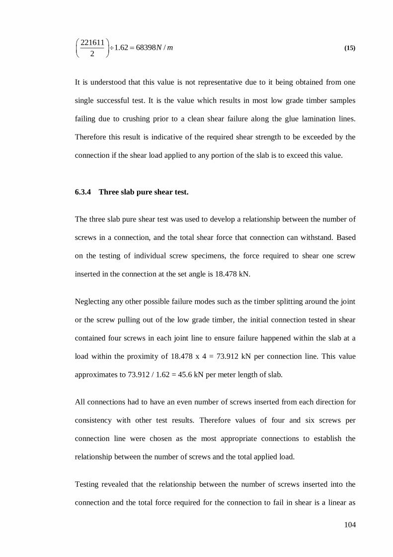
104
2216111.62 68398 /
2N m
(15)
It is understood that this value is not representative due to it being obtained from one
single successful test. It is the value which results in most low grade timber samples
failing due to crushing prior to a clean shear failure along the glue lamination lines.
Therefore this result is indicative of the required shear strength to be exceeded by the
connection if the shear load applied to any portion of the slab is to exceed this value.
6.3.4 Three slab pure shear test.
The three slab pure shear test was used to develop a relationship between the number of
screws in a connection, and the total shear force that connection can withstand. Based
on the testing of individual screw specimens, the force required to shear one screw
inserted in the connection at the set angle is 18.478 kN.
Neglecting any other possible failure modes such as the timber splitting around the joint
or the screw pulling out of the low grade timber, the initial connection tested in shear
contained four screws in each joint line to ensure failure happened within the slab at a
load within the proximity of 18.478 x 4 = 73.912 kN per connection line. This value
approximates to 73.912 / 1.62 = 45.6 kN per meter length of slab.
All connections had to have an even number of screws inserted from each direction for
consistency with other test results. Therefore values of four and six screws per
connection line were chosen as the most appropriate connections to establish the
relationship between the number of screws and the total applied load.
Testing revealed that the relationship between the number of screws inserted into the
connection and the total force required for the connection to fail in shear is a linear as

105
shown in Figure 61. The data points in this graph are derived from the maximum force
values obtained in section 6.2.5. As can be seen in this graph, the abundance of
variables present within low grade timber appears to have little effect on the consistency
of results obtained.
The results obtained were converted into units per meter length of slab for ease of
interpretation and design based on Figure 61. This chart is intended for a slab loaded
between two free slabs to create a shear loading on the joint. Therefore the total number
of screws required per connection should be halved to ensure that the distribution of
screws within the two connection lines is even.
Figure 61 – Floor slab connections design chart.

106
A variety of failure modes occurred within the connection under shear, with the shear
failure of individual screws being the main failure mechanism. The other source of
weakness in the connection subjected to shear is the timber splitting through the counter
sunk hole resulting in an effective shear failure.
Inspection of screws that did not fail fully in shear showed signs of a point of contra
flexion developing at the interface between slab units. This would later be the point
where shear failure occurred if more of the total load applied was distributed onto that
screw. The reason for some screws not shearing off completely is the composition of the
low grade timber surrounding the area where the screw in question is located, which
allows local crushing around the screw, or splitting of the timber which houses the
screw in position.
The pull out capacity of the batten screws was not exceeded in any connection test
undertaken which indicates that shear is the major contributing factor in the strength of
the joint. The relationship between the screws in a combination of tension and shear,
and a combination of compression and shear requires a more detailed analysis in order
to get a complete data set which fully describes the characteristics of a bugle head
batten screw used as a connection alternative between low grade slab units.
The loading situation on a floor slab is not definite and can arise in a number of
different manners dependent on the floor usage. The requirement for a floor to reach a
set un - supported span will result in the bending force always being present within
connections, and shear forces of considerable magnitude when large point loads such as
piano legs are supported by low grade timber slabs.

107
6.4 Conclusions
Connections comprised of skewed 14G 125 mm bugle head batten screws can be made
to exceed the capacity of the slab subjected to bending or shear. The design aid created
for constructing appropriate connections between slab units presents a method of
creating a connection with ample capacity to resist any force which is within the
capacity range of the slab units themselves.
Although this is adequate for construction, it is based only on physical test results which
show that the screws will fail in shear before the pull out capacity is reached. The shear
capacity of a skewed bugle head batten screw is a function of the angle that it is inserted
at, and hence the area of the elliptical shear plane created. The variation of the shear
capacity within a screw subjected to a combination of shear and tensile / compressive
forces is not fully understood, however analysis of the joint has revealed that this
situation is present within a connection between slab units. Further analysis on this type
of connection needs to be undertaken to develop a suitable theoretical method of
calculating the required spacing and orientation of screws in order to exceed the
predicted forces between individual slab units.
Investigation on connections between slab units has also shown that the direction of the
growth rings in each individual member affect the ability of the slab to take loads in a
two way bending situation. The direction of growth rings also contributes significantly
to the capacity of a slab unit subjected to shear forces. The variability of the timber
properties within a low grade timber slab also effect connection performance and should
be investigated completely for use with theoretical connection design.

108
Chapter 7
Conclusions
7.0 Summary
This research project has investigated the structural performance of low grade timber
laminated into slab units to be used as a flooring system. A full analysis from the
behaviour of individual members and slab units through to the performance of slab units
connected to form a floor slab has been investigated with the intention of determining
the limitations of using low grade timber slabs in flooring applications.
A combination of analysed test results and modelling revealed that the critical limiting
factor associated with low grade timber slabs used in a flooring application is
deflection. A full analysis of various loading situations and clear floor spans has been

109
undertaken to develop a deflection based design chart for low grade timber slabs applied
to flooring applications.
The testing of connections between individual slab units has proven that a connection
can be made which exceeds the strength of the slab in any combination of forces
applied. Further testing and analysis provided a simplified method of joint design based
on the load applied per meter length of the slab.
7.1 Achievement of project objectives
The following objectives have been addressed:
Reviewing the current use of laminated timber building technologies in other countries,
to gain an understanding and appreciation of current technologies.
A literature review has been undertaken to examine prior work done on different
facades of timber floor slabs which are created from individual laminated low grade
timber members. Due to this paper being the first on the use of low grade timber being
used in slabs as a flooring alternative, no literature has been found which can be used as
a comparison to my findings.
Extensive work has been undertaken in the use of timber bulk timber laminated into a
cross laminated product consisting of three or more layers, and the effects that timber
quality and using glue lamination has on the over length of a structure comprised of
such materials. Although it is clear that a sufficient amount of work has been done in
the use of bulk timber members to act as structural elements based on company product
marketing literature, research papers are not able to be interpreted due to the abundance
of Scandinavian and German dialect used to compose these papers. Further information

110
the various aspects of using laminated low grade timber as a floor slab alternative can
be found in Chapter 2.
Acquisition of timber material properties data from Hyne with the aim of using a
statistically representative set of data for the prediction of the slab behaviour during
testing.
The timber material properties that are a valid sample for the source of the low grade
timber used in the slab was obtained from Hyne for use in modelling the behaviour of
low grade timber slab floors subjected to loading. Evidence of this can be seen in Table
5 and Appendix D. Extra information has also been obtained from Timber Queensland
from a large database on the properties of Australian hardwoods which was used for the
Grey Ironbark properties in the Strand7 parametric modelling shown in chapter 5.
Collect structural performance data by testing prefabricated timber slabs.
The characteristics of single low grade timber members and laminated low grade timber
slabs were determined as a result of the testing work shown in Chapters 3 and 4. The
major difference observed between the low grade timber members and the slab units
comprising of low grade timber is the increase in consistency of the load deflection
relationship.
The numerical results obtained and the observations taken from the behaviour of both
forms of low grade timber display the fact that the glue used in the lamination of
individual members to form low grade slab units is responsible for creating a load
sharing system around areas of defects within individual members. This results in a
significantly decreased variation in the load – deflection characteristics observed in the
low grade timber slab units compared to that of individual low grade timber members.

111
Create mathematical computer models of the above ground flooring system using
Strand7 to extrapolate data on the structural requirements for this system to be viable.
Chapter 5 focussed on the selection of appropriate modelling parameters, and the
creation and use of Strand7 finite element analysis computer models to analyse the
limitations of using low grade timber slabs as a flooring alternative. Results from this
modelling highlighted that serviceability is the governing criteria in the design of floor
slabs constructed out of low grade timber.
Multiple span and load comparisons were also undertaken for a low grade slab model
and a standard flooring model in order to determine if the performance of the low grade
slab units used a flooring method are viable compared to that of the current standard
construction. This analysis was taken from a structural performance view point and
concluded that the low grade slab has a greater weight than the standard flooring
system, however the deflection response to all loading and span situations is less than
that of the standard floor constructed out of bearers, joists and a flooring material.
Use the results from modelling to create a design aid for the use of low grade timber
slabs in floor construction.
The structural characteristics of low grade timber floor slabs were obtained in Chapter
4. This information was incorporated in a range of Strand7 models as described in
Chapter 5. These models were then used to collected load and maximum deflection data
points over various spans with consistent loads applied. The result is a deflection based
design chart for 90 mm deep floor slabs subjected to a variety of different load cases.
Due to deflection being the limiting criteria in the design of low grade timber floor
slabs, deflections limit lines are superimposed on the chart so that it can be interpreted
in accordance with the required deflection limit used in design.

112
Investigate, create and test methods for panel connection.
The investigation of connections subjected to the forces which occur between slab units
is evident in module 6. Investigations revealed that it is possible to create a connection
that exceeds the strength of both the low grade timber and the glue lamination lines
between individual slab unit members. Investigations have also determined that there is
a linear relationship between the number of bugle head batten screws in a joint, and the
total shear force which the connection can withstand. Simplification of the connection
and the use of this physical test has resulted in the creation of a connection design chart
which can be used to determine the minimum number of screws required to resist a total
shear applied load.
7.2 Major findings
As a result of the research work undertaken, the following major findings have been
established:
Low grade timber members subjected to loading are highly unpredictable due to
the presence of excessive defects within the timber
Low grade timber laminated into floor slab units results in a product which is
very predictable when a load is applied, with a much smaller variation in results
than that of individual members

113
Extra head room is created as a result of the joists and flooring material being
replaced by the slab.
Low grade timber slabs are capable of taking loads with reliability that are
typically endured by flooring systems when the span is within the determined
limits.
Low grade timber slabs compare favourably to the standard floor construction
method of bearers joists and flooring materials based on the smaller deflection
obtained from the low grade slab model. The disadvantage is the increased
weight of the structure due to the bulk of timber used.
Connections can be made between slab units which are sufficient to endure the
loads that low grade timber slabs are capable of carrying. This allows floors of
any desired width to be created from a group of low grade slab units placed side
by side which acts as one single slab.
7.3 Future Work
The findings resulting from this research highlight several areas that are crucial to floor
design and require further investigation. These factors have not been considered in this
research paper with the exception of connection design which was given some
simplified investigation to derive a set of proven realistic criterion for the connection of
low grade slab units.
Further analysis of the connection method is required to fully understand the behaviour
of low grade slab unit connections which is complex and still not understood in a
comprehensive manner.

114
It is recommended that the following items be given detailed investigation in order to
determine the commercial viability of using low grade timber slabs as a flooring
alternative in Australia.
Natural frequency
Creep effects
Moisture related effects on slab performance
Further investigation on connection design between slab units
Cost comparison
Effects of two way bending

115
References
Australian Building Codes Board, Building Code of Australia, Canberra, Australian Capital
Territory, viewed 9th
April 2009, <http://www.abcb.gov.au/>
Custdio, J., Broughton, J. & Cruz, H. (2009), „A Review of factors influencing the durability of
structural bonded timber joints‟, International Journal of Adhesion and Adhesives 29(2), 173 –
185.
Engineers Australia, „The institution of engineers Australia code of ethics 2000‟.
http://www.engineersaustralia.org.au/shadomx/apps/fms/fmsdownload.cfm?file_uuid=F064759
5-C7FE-7720-EA17_70AC27062E0B&siteName=ieaust.
Falk, R. H. & Colling, F. (1995), „Laminating Effects in Glued-Laminated Timber Beams‟,
Journal of Structural Engineering 121(12), 1858 – 1863.
Foliente, G. (1998), „Design of timber structures subjected to extreme loads‟, Progress in
Structural Engineering and Materials 1(3).
Forest and Wood Products Australia 2009, Melbourne, Victoria, viewed 18 April 2009,
<http://www.fwpa.com.au/>
Gsell, D., Feltrin, G., Schubert, S., Steiger, R. & Motavalli, M. (2007), „Cross-Laminated
Timber Plates: Evaluation and Verification of Homogenized Elastic Properties‟, Journal of
Structural Engineering 133(1), 133 – 138.
He, M., Lam, F. & Foschi, R. (2000), Numerical analysis of statically loaded three-dimensional
timber light-frame buildings, in „6th
World Conference on Timber Engineering, Whistler,
Canada‟.

116
Lam, F. (2001), „Modern structural wood products‟, Progress in Structural Engineering and
Materials. 3(3), 238 – 245.
Lee, J. & Kim, G. (2000), „Study on the estimation of the strength properties of structural glued
laminated timber I: determination of optimum MOE as input variable‟, Journal of Wood Science
46(2), 115 – 121.
MacKenzie, C 2009, ‘Program Proposal To Develop Ecopanel’ , Feasibility analysis, Timber
Queensland Ltd, viewed 20 March 2009 2000,
http://mail.timberqueensland.com.au/ftp/EcoSLAB%20Information/
Metriguard Inc 2009, Precision testing equipment for wood, Pullman, Washington USA, viewed
25th June 2009, <http://www.metriguard.com/>
Moody, R.C. & Hernandez, R. (1997), Engineered wood products – A guide for specifiers,
designers and users, PFS Research Foundation, Madison, WI.
Purbond 2009, Adhesives for modern timber construction, Switzerland, viewed 22 September
2009, <http://www.purbond.com/purbond/Australia-NewZealand/EN/Technology /Polyurethane
- PUR/>
Soltis, L. & Rammer, D. (1993), „Shear strength of unchecked glued-laminated beams‟, Forrest
Products Journal 53705(1), 51 – 57.
Standards Australia 2002, Timber Structures – Design Methods, AS 1720.1-2002, Standards
Australia, Sydney, viewed 05 April 2009, <http://www.saiglobal.com/online/autologin.asp>.

117
Standards Australia 1999, Residential timber-framed construction, AS 1684.1 - 1999, Standards
Australia, Sydney, viewed 21 July 2009, <http://www.saiglobal.com/online/autologin.asp>.
Standards Australia 1995, Methods of test for veneer and plywood, AS 2098.9-1995, Standards
Australia, Sydney, viewed 06 April 2009, <http://www.saiglobal.com/online/autologin.asp>.
Standards Australia 2008, Plywood - Structural, AS 2269.1-2008, Standards Australia, Sydney,
viewed 06 April 2009, <http://www.saiglobal.com/online/autologin.asp>.
Standards Australia 1992, Timber – Stress-graded – In-grade strength and stiffness evaluation,
AS 4063-1992, Standards Australia, Sydney, viewed 05 April 2009,
<http://www.saiglobal.com/online/autologin.asp>.
Standards Australia 2007, Timber – Bond performance of structural adhesives, AS 4364-2007,
Standards Australia, Sydney, viewed 30 July 2009,
<http://www.saiglobal.com/online/autologin.asp>.
Standards Australia 2003, Glued laminated structural timber, AS 1328.2-1998, Standards
Australia, Sydney, viewed 30 July 2009, <http://www.saiglobal.com/online/autologin.asp>.
The Engineered Wood Association - APA 2009, Wood University, Tacoma, Washington USA,
viewed 20 May 2009, <http://www.wooduniversity.org>

118
Appendix A
Project Specification

119
FACULTY OF ENGINEERING AND SURVEYING
ENG4111/4112 Research Project PROJECT SPECIFICATION
FOR: Cameron James Clifford Summerville TOPIC: Structural Performance of Low Grade Timber Slabs SUPERVISORS: Associate Professor Karu Karunasena SPONSORSHIP: Hyne Timber Faculty of Engineering and Surveying PROJECT AIM: To investigate the structural performance of above ground
Low Grade Timber Slab flooring systems and develop design criteria for slabs as a flooring alternative.
PROGRAMME: (Issue B, 28
th September 2009)
1. Research the current use of laminated timber building technologies in other countries.
2. Obtain timber material properties data from Hyne to obtain
statistically representative data related to low grade timber.
3. Collect structural performance data by testing prefabricated Low Grade Timber Slabs.
4. Create a mathematical computer model of the above
ground flooring system using Strand7 to extrapolate data on the structural requirements for this system to be viable.
5. Use the results from modelling to create a design aid for
the use of Low Grade Timber Slabs in Floor Construction.
6. Investigate, create and test methods for panel connection.
7. Submit an academic dissertation on the research. AGREED: __________________(student) _________________(supervisor) Date____/____/_______ Date____/____/_______

120
Appendix B
OH&S - Work Permit

121

122
Appendix C
OH&S – Purbond 514 MSDS

123

124

125

126
Appendix D
Hyne Tuan mill material property data.

127

128
Appendix E
Timber Queensland Grey Ironbark test data.

129
Grey Ironbark Test data from Timber Queensland
No Species Visual
Grading MOE (GPa)
MOR (GPa)
Moisture Content (%)
Density (kg/m³)
0577 GRI R 17.29 91.85 green 1135
0722 GRI R 19.11 97.62 green 1099
0573 GRI 27 16.11 85.06 green 1130
0574 GRI 27 16.23 79.04 green 1136
0575 GRI 27 17.27 72.44 green 1134
0576 GRI 27 15.79 83.36 green 1114
0716 GRI 27 19.94 98.47 green 1130
0718 GRI 27 18.09 109.75 green 1060
0719 GRI 27 17.86 102.66 green 1073
0721 GRI 27 19.86 106.66 green 1121
1119 GRI 27 19.65 102.61 green 1064
1120 GRI 27 19.91 104.20 green 1071
0499 GRI R 19.46 92.77 green 1128
0497 GRI 27 21.13 94.11 green 1120
0720 GRI 27 20.71 112.80 green 1092
0496 GRI 27 - 112.54 green 1143
0717 GRI 27 - 106.72 green 1105
1119 GRI 34 14.65 105.77 15 972
1120 GRI 34 25.00 127.73 14 1072
0577 GRI 34 17.78 53.42 16 1162
0722 GRI 34 19.74 135.20 17 1100
0721 GRI R 19.61 109.54 14 1090
0573 GRI 34 14.56 75.70 16 1092
0574 GRI 34 16.54 93.84 16 1098
0575 GRI 34 15.43 78.92 14 1096
0716 GRI 34 19.99 131.57 16 1092
0718 GRI 34 20.23 120.63 16 1074
0717 GRI 34 16.77 90.71 17 1074
0719 GRI 34 18.11 71.43 20 1082
0720 GRI R 15.85 93.36 15 1079
0497 GRI 34 21.10 103.29 15 1153
0496 GRI 34 20.46 111.52 15 1177
0576 GRI 34 14.79 90.60 16 1076
0414 GRI 27 22.84 117.26 green 1135
0608 GRI 27 19.39 113.00 green 1124
0653 GRI 27 19.89 101.46 green 1185
0660 GRI 27 23.74 113.67 green 1171
0661 GRI 27 23.33 114.94 green 1164
0666 GRI 27 22.28 106.90 green 1127
0860 GRI R 19.55 96.20 green 1204
0654 GRI 27 21.23 98.04 green 1170
0856 GRI R 20.35 114.59 green 1133
0862 GRI 27 17.86 60.80 green 1216
1093 GRI R 7.06 25.12 green 1194
1091 GRI 22 12.67 64.52 green 1148
0412 GRI 27 23.18 118.93 green 1135
0853 GRI R 17.10 72.94 green 1231
0655 GRI 27 21.82 105.95 green 1169
0413 GRI 27 22.54 120.14 green 1110
0657 GRI 27 21.53 110.04 green 1191
0662 GRI 27 22.39 114.96 green 1168

130
0667 GRI 27 23.51 108.79 green 1185
0410 GRI R 21.66 116.82 green 1127
0411 GRI 27 21.30 118.65 green 1137
0663 GRI 27 20.06 115.40 green 1150
0857 GRI 27 19.83 116.65 green 1221
0418 GRI R 21.86 116.16 green 1120
0419 GRI R 22.56 110.31 green 1140
0604 GRI 27 20.61 102.55 green 1147
0605 GRI 27 19.34 96.52 green 1119
0606 GRI 27 19.85 100.55 green 1145
0607 GRI 27 20.78 104.52 green 1125
0609 GRI 27 17.27 94.33 green 1121
0656 GRI 27 21.00 115.15 green 1140
0664 GRI 27 25.07 123.11 green 1141
0665 GRI 27 22.02 126.51 green 1187
0849 GRI 27 20.02 118.19 green 1192
0850 GRI 27 20.10 100.30 green 1210
0851 GRI 27 15.87 95.62 green 1206
0859 GRI 27 19.43 114.10 green 1228
0603 GRI 27 15.45 101.30 green 1170
0658 GRI 27 17.12 113.05 green 1187
0659 GRI 27 20.70 115.65 green 1195
0409 GRI 27 23.06 118.88 green 1131
0602 GRI 27 21.30 102.97 green 1150
0852 GRI R 19.77 105.05 green 1204
1092 GRI R 11.76 32.77 green 1156
1089 GRI 22 12.97 78.47 green 1212
1090 GRI 22 13.64 83.81 green 1156
1096 GRI 27 14.14 81.25 green 1145
1088 GRI R 14.84 87.91 green 1172
1094 GRI 27 12.99 77.44 green 1183
1095 GRI 27 13.99 72.16 green 1189
1097 GRI 27 12.47 71.91 green 1162
1098 GRI 27 11.20 67.16 green 1178
0859 GRI R 20.99 90.70 12 1187
1089 GRI 43 13.59 57.05 10 1100
0853 GRI R 21.83 131.25 12 1263
0418 GRI R 23.15 123.07 11 1131
1095 GRI 43 4.52 13.18 11 1089
0656 GRI 43 24.48 100.87 13 1126
0852 GRI 43 25.64 137.68 12 1212
0664 GRI 34 21.47 96.99 14 1075
0411 GRI 34 23.68 106.81 11 1088
1094 GRI R 13.90 66.87 14 1111
1090 GRI 34 14.48 62.53 11 1112
0851 GRI 43 15.55 139.13 13 1213
0666 GRI R 21.24 80.55 12 1099
0654 GRI 34 23.69 127.47 12 1107
0413 GRI 34 21.90 105.59 12 1033
0412 GRI 43 26.83 155.72 11 1121
0603 GRI 43 24.26 127.09 13 1138
0606 GRI 43 26.62 154.21 14 1152
0659 GRI 43 25.57 155.30 12 1143
0849 GRI 43 23.33 136.18 13 1186

131
0419 GRI 43 25.54 119.32 12 1118
0604 GRI 43 24.94 135.75 12 1134
0605 GRI 43 26.40 143.27 13 1127
0608 GRI 43 26.21 137.32 12 1142
0661 GRI 43 23.46 149.96 12 1153
0665 GRI 43 - 123.60 12 1086
0667 GRI 43 20.24 116.39 13 889
0860 GRI 43 24.04 113.93 12 1227
0862 GRI 43 21.19 90.31 12 1162
1097 GRI 43 14.16 76.03 10 1078
0856 GRI 43 20.87 141.39 12 1151
0857 GRI 43 20.78 95.69 11 1209
1088 GRI R 16.59 70.20 10 1085
0410 GRI 34 24.19 65.64 13 1089
0655 GRI 34 22.95 63.50 15 1139
0850 GRI R 9.44 18.25 12 1079
0609 GRI 43 24.27 118.75 15 1149
0653 GRI 34 25.09 136.56 13 1080
0663 GRI 27 19.79 61.47 15 1085
0409 GRI 34 20.76 37.25 13 1103
0660 GRI 34 24.48 123.49 11 1104
0607 GRI 27 24.00 137.36 13 1079
0662 GRI 27 25.85 100.04 12 1109
1091 GRI 43 12.41 56.27 11 1047
0414 GRI R 22.65 123.23 13 1033
0602 GRI 43 22.31 149.60 11 1089
0657 GRI R 24.02 129.55 12 1114
0658 GRI 43 25.12 151.03 15 1138
1098 GRI 43 13.54 60.93 10 1102
1096 GRI R 16.33 78.57 10 1066
1093 GRI 43 15.90 63.54 11 1029
1093 GRI R 9.51 38.66 10 1069

132
Appendix F
Slab unit connection ideas.

133
IDEA 1 – Single high grade timber plank face jointed into adjacent slab units
IDEA 2 – A plank spanning the length of the slab with nails or screws driven directly into each
member

134
IDEA 3 – A large dovetail block fixed into a pre-cut joint in the slabs.
IDEA 4 – 140 mm deep laminates on the outside edges of each slab unit with bolts connecting them
together underneath the slab

135
IDEA 5 – Bugle head batten screws skewed into the slabs and counter sunk below the surface.

136
Appendix G
Matlab code used to analyse recorded data

137
G.1 – Matlab code used to plot test results.
clear clc format short g
% timber sample properties
B = 35*12; D = 90; L = 1620; a = L/3 n = (((3*a)/(4*L))-((a/L)^3))
%_____________________________________________________________________
Sample_n = xlsread('CAMERON - S1A') N = size(Sample_n(:,3));
P2 = (Sample_n(floor((N(1,1)-(N(1,1)/2))),5)); P1 = (Sample_n(floor((0+(N(1,1)/9))),5));
P_diff = P2/2-P1/2;
D2 = (Sample_n(floor((N(1,1)-N(1,1)/2)),3)); D1 = (Sample_n(floor((0+N(1,1)/9)),3));
D_diff = D2-D1;
E1 = (((2*n*L.^3)/(B*D.^3))* (P_diff/D_diff))
hold on plot(Sample_n(:,3),(Sample_n(:,4)*1000), 'r') hold on
%_____________________________________________________________________
Sample_n = xlsread('CAMERON - S1B') N = size(Sample_n(:,3));
P2 = (Sample_n(floor((N(1,1)-(N(1,1)/2))),5)); P1 = (Sample_n(floor((0+(N(1,1)/9))),5));
P_diff = P2/2-P1/2;
D2 = (Sample_n(floor((N(1,1)-N(1,1)/2)),3)); D1 = (Sample_n(floor((0+N(1,1)/9)),3));
D_diff = D2-D1;
E2 = (((2*n*L.^3)/(B*D.^3))* (P_diff/D_diff))
hold on plot(Sample_n(:,3),(Sample_n(:,4)*1000), 'g') hold on

138
%_____________________________________________________________________
Sample_n = xlsread('CAMERON - S2A') N = size(Sample_n(:,3));
P2 = (Sample_n(floor((N(1,1)-(N(1,1)/2))),5)); P1 = (Sample_n(floor((0+(N(1,1)/9))),5));
P_diff = P2/2-P1/2;
D2 = (Sample_n(floor((N(1,1)-N(1,1)/2)),3)); D1 = (Sample_n(floor((0+N(1,1)/9)),3));
D_diff = D2-D1;
E3 = (((2*n*L.^3)/(B*D.^3))* (P_diff/D_diff))
hold on plot(Sample_n(:,3),(Sample_n(:,4)*1000), 'b') hold on
%_____________________________________________________________________
Sample_n = xlsread('CAMERON - S2B') N = size(Sample_n(:,3));
P2 = (Sample_n(floor((N(1,1)-(N(1,1)/2))),5)); P1 = (Sample_n(floor((0+(N(1,1)/9))),5));
P_diff = P2/2-P1/2;
D2 = (Sample_n(floor((N(1,1)-N(1,1)/2)),3)); D1 = (Sample_n(floor((0+N(1,1)/9)),3));
D_diff = D2-D1;
E4 = (((2*n*L.^3)/(B*D.^3))* (P_diff/D_diff))
hold on plot(Sample_n(:,3),(Sample_n(:,4)*1000), 'm') hold on
%_____________________________________________________________________
Sample_n = xlsread('CAMERON - S3A') N = size(Sample_n(:,3));
P2 = (Sample_n(floor((N(1,1)-(N(1,1)/2))),5)); P1 = (Sample_n(floor((0+(N(1,1)/9))),5));
P_diff = P2/2-P1/2;
D2 = (Sample_n(floor((N(1,1)-N(1,1)/2)),3)); D1 = (Sample_n(floor((0+N(1,1)/9)),3));

139
D_diff = D2-D1;
E5 = (((2*n*L.^3)/(B*D.^3))* (P_diff/D_diff))
hold on plot(Sample_n(:,3),(Sample_n(:,4)*1000), 'y') hold on
%_____________________________________________________________________
Sample_n = xlsread('CAMERON - S3B') N = size(Sample_n(:,3));
P2 = (Sample_n(floor((N(1,1)-(N(1,1)/2))),5)); P1 = (Sample_n(floor((0+(N(1,1)/9))),5));
P_diff = P2/2-P1/2;
D2 = (Sample_n(floor((N(1,1)-N(1,1)/2)),3)); D1 = (Sample_n(floor((0+N(1,1)/9)),3));
D_diff = D2-D1;
E6 = (((2*n*L.^3)/(B*D.^3))* (P_diff/D_diff))
hold on plot(Sample_n(:,3),(Sample_n(:,4)*1000), 'k') hold on
%_____________________________________________________________________
_____
ylabel('Load (N)','fontsize',14) xlabel('Deflection (mm)','fontsize',14) title ('Timber Slab Test Results','fontsize',14) h = legend('SAMPLE 1A','SAMPLE 1B','SAMPLE 2A','SAMPLE 2B','SAMPLE
3A','SAMPLE 3B',2); grid on
Average = (E1+E2+E3+E4+E5+E6)/6

140
G.2 – Matlab code used to calculate Modulus of Elasticity clear clc format short g
% timber sample properties
B = 35*12; D = 90; L = 1620; a = L/3 n = (((3*a)/(4*L))-((a/L)^3))
%_____________________________________________________________________
alpha = 1; while alpha <12
document = uigetfile('*.xls','Open data file'); Sample_n = xlsread(document) display(document) N = size(Sample_n(:,3));
P2 = (Sample_n(floor((N(1,1)-(N(1,1)/2))),5)); P1 = (Sample_n(floor((0+(N(1,1)/9))),5));
P_diff = P2/2-P1/2;
D2 = (Sample_n(floor((N(1,1)-N(1,1)/2)),3)); D1 = (Sample_n(floor((0+N(1,1)/9)),3));
D_diff = D2-D1;
E = (((2*n*L.^3)/(B*D.^3))* (P_diff/D_diff))
LOBF = [P2, P1;D2,D1]; figure('Position',get(0,'ScreenSize')) plot(LOBF(2,:),LOBF(1,:),'b-*','markersize', 20,'linewidth', 2) hold on plot(Sample_n(:,3),Sample_n(:,5), 'r') hold on
x_coord = Sample_n(N(1,1),3)/2; y_coord = Sample_n(N(1,1),5)/2;
text(x_coord,y_coord,num2str(E),'fontsize', 16,'fontweight', 'bold')
ylabel('Load (N)','fontsize',14) xlabel('Deflection (mm)','fontsize',14) title ('Test Results Analysis','fontsize',14) h = legend('Modulus of Elasticity (MPa)',document,2); grid on %print('-djpeg100',document) pause
alpha = alpha + 1 end
G.3 – Matlab code used to plot design chart

141
clear; clc; LOAD_DATA =
[0,3.460399412,6.489,9.949399412,16.43839941,22.92739941,29.41639941,3
5.90539941;%,52.12789941;
0,4.613865883,8.652,13.26586588,21.91786588,30.56986588,39.22186588,47
.87386588;%,69.50386588;
0,5.767332354,10.815,16.58233235,27.39733235,38.21233235,49.02733235,5
9.84233235;%,86.87983235;
0,6.920798825,12.978,19.89879882,32.87679882,45.85479882,58.83279882,7
1.81079882;%,104.2557988;
0,8.074265296,15.141,23.2152653,38.3562653,53.4972653,68.6382653,83.77
92653;%,121.6317653;
0,9.227731766,17.304,26.53173177,43.83573177,61.13973177,78.44373177,9
5.74773177;%,139.0077318;
0,10.38119824,19.467,29.84819824,49.31519824,68.78219824,88.24919824,1
07.7161982;%,156.3836982;
0,11.53466471,21.63,33.16466471,54.79466471,76.42466471,98.05466471,11
9.6846647]%,173.7596647]
DEFLECTION_DATA = [0,0,0,0,0,0,0,0; 0.4,0.5,1.1,2.3,4.2,7.1,11.3,17.1; 0.3,0.8,2,4.2,7.7,13,21,31.9; 0.7,1.3,3.1,6.4,11.9,20.1,32.2,49; 0.9,2.1,5.1,10.6,19.6,33.1,53.2,80.9; 1.2,2.9,7.2,14.8,27.3,46,74.2,112.7; 1.5,3.8,9.2,19,35,59,95.1,144.6; 1.7,4.6,11.2,23.2,42.8,72,116.1,176.4;] %2.4,6.7,16.3,33.6,62.1,104.5,168.5,256.1] for i = 1:8 plot(DEFLECTION_DATA(:,i),LOAD_DATA(i,:),'-r*') hold on end
for i = 1:8 plot(DEFLECTION_DATA(i,:),LOAD_DATA(:,i),'-b') hold on end
for n = 1:8 gradient(1,n) = LOAD_DATA(n,8)/DEFLECTION_DATA(8,n); hold on end gradient
Lmark = 1; for L = 1800:600:6000 %xLon400(1,Lmark)= L/400; xLon360(1,Lmark) = L/360; %xLon300(1,Lmark) = L/300; xLon250(1,Lmark) = L/250; %xLon200(1,Lmark) = L/200; xLon150(1,Lmark) = L/150; xLon100(1,Lmark) = L/100; Lmark = Lmark + 1; end

142
%xLon = [xLon400;xLon350;xLon300;xLon250;xLon200;xLon150;xLon100] xLon = [xLon360;xLon250;xLon150;xLon100]
g_mark = 1;%2; for column_mark = 1:8 for row_mark = 1:4
yLon(row_mark,column_mark) = xLon(row_mark,column_mark) *
gradient(1,g_mark); end g_mark = g_mark + 1; end
yLon for xplot = 1:8 for yplot = 1:4
%if yLon(yplot,xplot) < LOAD_DATA(yplot,xplot)+60 %xplot(yplot,xplot) = xLon(yplot,xplot) %yplot(yplot,xplot) = yLon(yplot,xplot) %plot(xLon(yplot,xplot),yLon(yplot,xplot),'-g*') plot(xLon(yplot,:),yLon(yplot,:),'-g*')
hold on
% end end end
ylim([0 120]) grid on ylabel('Total Load (kN) (Including Self Weight)','fontsize',14) xlabel('Deflection (mm)','fontsize',14) title ('Load / Deflection Limit Graphs for LOW GRADE
SLAB','fontsize',14)

143
G.4 – Matlab code used to plot stress limit graphs clear clc SPAN_1 = 3600; SPAN_2 = 6000;
%______________________DEFLECTIONS____________________________________
_____ Stress_Lim_SLAB = [35714,35714]; Stress_Lim_NORM = [80000,80000] %_______________3.6 m x 3.6 m Slab____________________________________
Load_One_t =
[0,7.889,12.96,20.849,33.809,46.769,59.729,72.689,105.089];; Stress_One_t =
[0,701.8559,1247.9872,1949.8431,3197.8302,4445.8174,5693.8045,6941.791
7,10061.7596];
plot(Stress_One_t, Load_One_t,'b--*')
hold on %_______________3.6 m x 3.6 m
Standard____________________________________
Load_Two_t =
[0,4.696,12.96,17.656,30.616,43.576,56.536,69.496,101.896]; Stress_Two_t =
[0,1833.6946,6240.0804,8073.77550,14313.8554,20553.9358,26794.0162,330
34.0966,48634.2976];
Drawing_Limit = [0,max(Load_One_t)];
plot(Stress_Two_t, Load_Two_t,'m--*'); hold on
plot(Stress_Lim_SLAB,Drawing_Limit,'b');
hold on
plot(Stress_Lim_NORM,Drawing_Limit,'m');
hold on
ylabel('Total Load (kN) (Including Self Weight)','fontsize',14) xlabel('Stress (kPa)','fontsize',14) title ('Timber Flooring Stress Limits 3.6m span','fontsize',14) h = legend('3.6m x 3.6m Slab','3.6m x 3.6m Standard','Stress
Limit',2); grid on
figure
%_______________6 m x 3.6 m Slab____________________________________
Load_One_s =
[0,12.503,21.6,34.103,55.703,77.303,98.903,120.503,174.503];

144
Stress_One_s =
[0,1671.3984,3048.7292,4720.1276,7768.8569,10817.5861,13866.3153,16915
.0445,24536.8676];
plot(Stress_One_s, Load_One_s,'b--*')
hold on %_______________6 m x 3.6 m
Standard____________________________________
Load_Two_s =
[0,7.2387,21.6,28.8387,50.4387,72.0387,93.6387,115.2387,169.2387]; Stress_Two_s =
[0,4102.7515,14024.84,18125.2787,32149.0627,46173.9029,60198.7431,7422
3.5834,109285.6839];
Drawing_Limit = [0,max(Load_One_s)];
plot(Stress_Two_s, Load_Two_s,'m--*')
hold on
plot(Stress_Lim_SLAB,Drawing_Limit,'b')
hold on
plot(Stress_Lim_NORM,Drawing_Limit,'m')
hold on
ylabel('Total Load (kN) (Including Self Weight)','fontsize',14) xlabel('Stress (kPa)','fontsize',14) title ('Timber Flooring Stress Limits for 6m span','fontsize',14) h = legend('6m x 3.6m Slab','6m x 3.6m Standard','Stress Limit',2); grid on
%_____________COMPARISON OF STRESSES ON STANDARD FLOORING
SETUP___________%
figure
%Load Case 1 %STRESS_COMPARISONa = [Stress_Two_s(1),Stress_Two_t(1)] %LOAD_COMPARISONa = [Load_Two_s(1),Load_Two_t(1)] %plot(STRESS_COMPARISONa, LOAD_COMPARISONa,'r--*') %hold on
%Load Case 1 STRESS_COMPARISONa = [Stress_Two_s(2),Stress_Two_t(2)]; LOAD_COMPARISONa = [Load_Two_s(2),Load_Two_t(2)]; plot(STRESS_COMPARISONa, LOAD_COMPARISONa,'b--*') if STRESS_COMPARISONa(2) < Stress_Lim_NORM(1) if STRESS_COMPARISONa(1) > Stress_Lim_NORM(1) CASE ='Slab Stress Limit' UNKNOWN_SPAN_LC1js = ( ( (LOAD_COMPARISONa(1) -
LOAD_COMPARISONa(2))* (Stress_Lim_NORM(1) -
STRESS_COMPARISONa(2)))/... (STRESS_COMPARISONa(1)-
STRESS_COMPARISONa(2)) ) + LOAD_COMPARISONa(2); hold on

145
plot(Stress_Lim_NORM(1),UNKNOWN_SPAN_LC1,'bd') SLAB_LENGTH_LC1 = (((SPAN_2-SPAN_1)*(UNKNOWN_SPAN_LC1 -
LOAD_COMPARISONa(2)))/... (LOAD_COMPARISONa(1) - LOAD_COMPARISONa(2))) + SPAN_1 end end
hold on
%Load Case 2 STRESS_COMPARISONa = [Stress_Two_s(3),Stress_Two_t(3)]; LOAD_COMPARISONa = [Load_Two_s(3),Load_Two_t(3)]; plot(STRESS_COMPARISONa, LOAD_COMPARISONa,'g--*') if STRESS_COMPARISONa(2) < Stress_Lim_NORM(1) if STRESS_COMPARISONa(1) > Stress_Lim_NORM(1) UNKNOWN_SPAN_LC2 = ( ( (LOAD_COMPARISONa(1) -
LOAD_COMPARISONa(2))* (Stress_Lim_NORM(1) -
STRESS_COMPARISONa(2)))/... (STRESS_COMPARISONa(1)-
STRESS_COMPARISONa(2)) ) + LOAD_COMPARISONa(2); hold on plot(Stress_Lim_NORM(1),UNKNOWN_SPAN_LC2,'gd') SLAB_LENGTH_LC2js = (((SPAN_2-SPAN_1)*(UNKNOWN_SPAN_LC2 -
LOAD_COMPARISONa(2)))/... (LOAD_COMPARISONa(1) - LOAD_COMPARISONa(2))) + SPAN_1 end end hold on
%Load Case 3 STRESS_COMPARISONa = [Stress_Two_s(4),Stress_Two_t(4)]; LOAD_COMPARISONa = [Load_Two_s(4),Load_Two_t(4)]; plot(STRESS_COMPARISONa, LOAD_COMPARISONa,'c--*') if STRESS_COMPARISONa(2) < Stress_Lim_NORM(1) if STRESS_COMPARISONa(1) > Stress_Lim_NORM(1) UNKNOWN_SPAN_LC3 = ( ( (LOAD_COMPARISONa(1) -
LOAD_COMPARISONa(2))* (Stress_Lim_NORM(1) -
STRESS_COMPARISONa(2)))/... (STRESS_COMPARISONa(1)-
STRESS_COMPARISONa(2)) ) + LOAD_COMPARISONa(2); hold on plot(Stress_Lim_NORM(1),UNKNOWN_SPAN_LC3,'cd') SLAB_LENGTH_LC3js = (((SPAN_2-SPAN_1)*(UNKNOWN_SPAN_LC3 -
LOAD_COMPARISONa(2)))/... (LOAD_COMPARISONa(1) - LOAD_COMPARISONa(2))) + SPAN_1 end end hold on
%Load Case 4 STRESS_COMPARISONa = [Stress_Two_s(5),Stress_Two_t(5)]; LOAD_COMPARISONa = [Load_Two_s(5),Load_Two_t(5)]; plot(STRESS_COMPARISONa, LOAD_COMPARISONa,'m--*') if STRESS_COMPARISONa(2) < Stress_Lim_NORM(1) if STRESS_COMPARISONa(1) > Stress_Lim_NORM(1) UNKNOWN_SPAN_LC4 = ( ( (LOAD_COMPARISONa(1) -
LOAD_COMPARISONa(2))* (Stress_Lim_NORM(1) -
STRESS_COMPARISONa(2)))/... (STRESS_COMPARISONa(1)-
STRESS_COMPARISONa(2)) ) + LOAD_COMPARISONa(2); hold on plot(Stress_Lim_NORM(1),UNKNOWN_SPAN_LC4,'md')

146
SLAB_LENGTH_LC6js = (((SPAN_2-SPAN_1)*(UNKNOWN_SPAN_LC6 -
LOAD_COMPARISONa(2)))/... (LOAD_COMPARISONa(1) - LOAD_COMPARISONa(2))) + SPAN_1 end end hold on
%Load Case 5 STRESS_COMPARISONa = [Stress_Two_s(6),Stress_Two_t(6)]; LOAD_COMPARISONa = [Load_Two_s(6),Load_Two_t(6)]; plot(STRESS_COMPARISONa, LOAD_COMPARISONa,'r--o') if STRESS_COMPARISONa(2) < Stress_Lim_NORM(1) if STRESS_COMPARISONa(1) > Stress_Lim_NORM(1) UNKNOWN_SPAN_LC5 = ( ( (LOAD_COMPARISONa(1) -
LOAD_COMPARISONa(2))* (Stress_Lim_NORM(1) -
STRESS_COMPARISONa(2)))/... (STRESS_COMPARISONa(1)-
STRESS_COMPARISONa(2)) ) + LOAD_COMPARISONa(2); hold on plot(Stress_Lim_NORM(1),UNKNOWN_SPAN_LC5,'rd') SLAB_LENGTH_LC5js = (((SPAN_2-SPAN_1)*(UNKNOWN_SPAN_LC5 -
LOAD_COMPARISONa(2)))/... (LOAD_COMPARISONa(1) - LOAD_COMPARISONa(2))) + SPAN_1 end end hold on
%Load Case 6 STRESS_COMPARISONa = [Stress_Two_s(7),Stress_Two_t(7)]; LOAD_COMPARISONa = [Load_Two_s(7),Load_Two_t(7)];
plot(STRESS_COMPARISONa, LOAD_COMPARISONa,'b--o')
if STRESS_COMPARISONa(2) < Stress_Lim_NORM(1) if STRESS_COMPARISONa(1) > Stress_Lim_NORM(1) UNKNOWN_SPAN_LC6 = ( ( (LOAD_COMPARISONa(1) -
LOAD_COMPARISONa(2))* (Stress_Lim_NORM(1) -
STRESS_COMPARISONa(2)))/... (STRESS_COMPARISONa(1)-
STRESS_COMPARISONa(2)) ) + LOAD_COMPARISONa(2); hold on plot(Stress_Lim_NORM(1),UNKNOWN_SPAN_LC6,'bd') SLAB_LENGTH_LC6js = (((SPAN_2-SPAN_1)*(UNKNOWN_SPAN_LC6 -
LOAD_COMPARISONa(2)))/... (LOAD_COMPARISONa(1) - LOAD_COMPARISONa(2))) + SPAN_1 end end
hold on
%Load Case 7 STRESS_COMPARISONa = [Stress_Two_s(8),Stress_Two_t(8)]; LOAD_COMPARISONa = [Load_Two_s(8),Load_Two_t(8)]; plot(STRESS_COMPARISONa, LOAD_COMPARISONa,'g--o')
if STRESS_COMPARISONa(2) < Stress_Lim_NORM(1) if STRESS_COMPARISONa(1) > Stress_Lim_NORM(1) UNKNOWN_SPAN_LC7 = (((LOAD_COMPARISONa(1) -
LOAD_COMPARISONa(2))/(STRESS_COMPARISONa(1)-STRESS_COMPARISONa(2)))...

147
*(Stress_Lim_NORM(1) - STRESS_COMPARISONa(2)))+
LOAD_COMPARISONa(2); hold on plot(Stress_Lim_NORM(1),UNKNOWN_SPAN_LC7,'gd') SLAB_LENGTH_LC7js = (((SPAN_2-SPAN_1)*(UNKNOWN_SPAN_LC7 -
LOAD_COMPARISONa(2)))/... (LOAD_COMPARISONa(1) - LOAD_COMPARISONa(2))) + SPAN_1 end
%LOAD_COMPARISONa(2) = SPAN_1; %LOAD_COMPARISONa(1) = SPAN_2; end hold on %Load Case 1 %STRESS_COMPARISONa = [Stress_Two_s(9),Stress_Two_t(9)] %LOAD_COMPARISONa = [Load_Two_s(9),Load_Two_t(9)] %plot(STRESS_COMPARISONa, LOAD_COMPARISONa,'c--o') %hold on
plot(Stress_Lim_SLAB,Drawing_Limit,'r') hold on plot(Stress_Lim_NORM,Drawing_Limit,'b')
ylabel('Total Load (kN) (Including Self Weight)','fontsize',14) xlabel('Stress (kPa)','fontsize',14) title ('Comparison Between Standard 3.6m and 6m span for each Load
Case','fontsize',14) h = legend('Gravity','1kN/m^2','Gravity + 1kN/m^2','Gravity +
2kN/m^2','Gravity + 3kN/m^2'... ,'Gravity + 4kN/m^2','Gravity + 5kN/m^2','Limiting Stress',2); grid on
%_____________COMPARISON OF STRESSES ON SLAB FLOORING
SETUP___________%
figure
%Load Case 1 %STRESS_COMPARISONa = [Stress_One_s(1),Stress_One_t(1)] %LOAD_COMPARISONa = [Load_One_s(1),Load_One_t(1)] %plot(STRESS_COMPARISONa, LOAD_COMPARISONa,'r--*') %hold on %Load Case 1 STRESS_COMPARISONa = [Stress_One_s(2),Stress_One_t(2)]; LOAD_COMPARISONa = [Load_One_s(2),Load_One_t(2)]; plot(STRESS_COMPARISONa, LOAD_COMPARISONa,'b--*')
if STRESS_COMPARISONa(2) < Stress_Lim_SLAB(1) if STRESS_COMPARISONa(1) > Stress_Lim_SLAB(1) UNKNOWN_SPAN_LC1 = ( ( (LOAD_COMPARISONa(1) -
LOAD_COMPARISONa(2))* (Stress_Lim_SLAB(1) -
STRESS_COMPARISONa(2)))/... (STRESS_COMPARISONa(1)-
STRESS_COMPARISONa(2)) ) + LOAD_COMPARISONa(2); hold on plot(Stress_Lim_SLAB(1),UNKNOWN_SPAN_LC1,'bd') SLAB_LENGTH_LC1ss = (((SPAN_2-SPAN_1)*(UNKNOWN_SPAN_LC1 -
LOAD_COMPARISONa(2)))/... (LOAD_COMPARISONa(1) - LOAD_COMPARISONa(2))) + SPAN_1 end

148
end
hold on
%Load Case 2 STRESS_COMPARISONa = [Stress_One_s(3),Stress_One_t(3)]; LOAD_COMPARISONa = [Load_One_s(3),Load_One_t(3)]; plot(STRESS_COMPARISONa, LOAD_COMPARISONa,'g--*') if STRESS_COMPARISONa(2) < Stress_Lim_SLAB(1) if STRESS_COMPARISONa(1) > Stress_Lim_SLAB(1) UNKNOWN_SPAN_LC2 = ( ( (LOAD_COMPARISONa(1) -
LOAD_COMPARISONa(2))* (Stress_Lim_SLAB(1) -
STRESS_COMPARISONa(2)))/... (STRESS_COMPARISONa(1)-
STRESS_COMPARISONa(2)) ) + LOAD_COMPARISONa(2); hold on plot(Stress_Lim_SLAB(1),UNKNOWN_SPAN_LC2,'gd') SLAB_LENGTH_LC2ss = (((SPAN_2-SPAN_1)*(UNKNOWN_SPAN_LC2 -
LOAD_COMPARISONa(2)))/... (LOAD_COMPARISONa(1) - LOAD_COMPARISONa(2))) + SPAN_1 end end hold on
%Load Case 3 STRESS_COMPARISONa = [Stress_One_s(4),Stress_One_t(4)]; LOAD_COMPARISONa = [Load_One_s(4),Load_One_t(4)]; plot(STRESS_COMPARISONa, LOAD_COMPARISONa,'c--*') if STRESS_COMPARISONa(2) < Stress_Lim_SLAB(1) if STRESS_COMPARISONa(1) > Stress_Lim_SLAB(1) UNKNOWN_SPAN_LC3 = ( ( (LOAD_COMPARISONa(1) -
LOAD_COMPARISONa(2))* (Stress_Lim_SLAB(1) -
STRESS_COMPARISONa(2)))/... (STRESS_COMPARISONa(1)-
STRESS_COMPARISONa(2)) ) + LOAD_COMPARISONa(2); hold on plot(Stress_Lim_SLAB(1),UNKNOWN_SPAN_LC3,'cd') SLAB_LENGTH_LC3ss = (((SPAN_2-SPAN_1)*(UNKNOWN_SPAN_LC3 -
LOAD_COMPARISONa(2)))/... (LOAD_COMPARISONa(1) - LOAD_COMPARISONa(2))) + SPAN_1 end end hold on
%Load Case 4 STRESS_COMPARISONa = [Stress_One_s(5),Stress_One_t(5)]; LOAD_COMPARISONa = [Load_One_s(5),Load_One_t(5)]; plot(STRESS_COMPARISONa, LOAD_COMPARISONa,'m--*') if STRESS_COMPARISONa(2) < Stress_Lim_SLAB(1) if STRESS_COMPARISONa(1) > Stress_Lim_SLAB(1) UNKNOWN_SPAN_LC4 = ( ( (LOAD_COMPARISONa(1) -
LOAD_COMPARISONa(2))* (Stress_Lim_SLAB(1) -
STRESS_COMPARISONa(2)))/... (STRESS_COMPARISONa(1)-
STRESS_COMPARISONa(2)) ) + LOAD_COMPARISONa(2); hold on plot(Stress_Lim_SLAB(1),UNKNOWN_SPAN_LC4,'md') SLAB_LENGTH_LC4ss = (((SPAN_2-SPAN_1)*(UNKNOWN_SPAN_LC4 -
LOAD_COMPARISONa(2)))/... (LOAD_COMPARISONa(1) - LOAD_COMPARISONa(2))) + SPAN_1 end end hold on

149
%Load Case 5 STRESS_COMPARISONa = [Stress_One_s(6),Stress_One_t(6)]; LOAD_COMPARISONa = [Load_One_s(6),Load_One_t(6)]; plot(STRESS_COMPARISONa, LOAD_COMPARISONa,'r--o')
if STRESS_COMPARISONa(2) < Stress_Lim_SLAB(1) if STRESS_COMPARISONa(1) > Stress_Lim_SLAB(1) UNKNOWN_SPAN_LC5 = ( ( (LOAD_COMPARISONa(1) -
LOAD_COMPARISONa(2))* (Stress_Lim_SLAB(1) -
STRESS_COMPARISONa(2)))/... (STRESS_COMPARISONa(1)-
STRESS_COMPARISONa(2)) ) + LOAD_COMPARISONa(2); hold on plot(Stress_Lim_SLAB(1),UNKNOWN_SPAN_LC5,'rd') SLAB_LENGTH_LC5ss = (((SPAN_2-SPAN_1)*(UNKNOWN_SPAN_LC5 -
LOAD_COMPARISONa(2)))/... (LOAD_COMPARISONa(1) - LOAD_COMPARISONa(2))) + SPAN_1 end end hold on
%Load Case 6 STRESS_COMPARISONa = [Stress_One_s(7),Stress_One_t(7)]; LOAD_COMPARISONa = [Load_One_s(7),Load_One_t(7)]; plot(STRESS_COMPARISONa, LOAD_COMPARISONa,'b--o') if STRESS_COMPARISONa(2) < Stress_Lim_SLAB(1) if STRESS_COMPARISONa(1) > Stress_Lim_SLAB(1) UNKNOWN_SPAN_LC6 = ( ( (LOAD_COMPARISONa(1) -
LOAD_COMPARISONa(2))* (Stress_Lim_SLAB(1) -
STRESS_COMPARISONa(2)))/... (STRESS_COMPARISONa(1)-
STRESS_COMPARISONa(2)) ) + LOAD_COMPARISONa(2); hold on plot(Stress_Lim_SLAB(1),UNKNOWN_SPAN_LC6,'bd') SLAB_LENGTH_LC6ss = (((SPAN_2-SPAN_1)*(UNKNOWN_SPAN_LC6 -
LOAD_COMPARISONa(2)))/... (LOAD_COMPARISONa(1) - LOAD_COMPARISONa(2))) + SPAN_1 end end hold on
%Load Case 7 STRESS_COMPARISONa = [Stress_One_s(8),Stress_One_t(8)]; LOAD_COMPARISONa = [Load_One_s(8),Load_One_t(8)]; plot(STRESS_COMPARISONa, LOAD_COMPARISONa,'g--o')
if STRESS_COMPARISONa(2) < Stress_Lim_SLAB(1) if STRESS_COMPARISONa(1) > Stress_Lim_SLAB(1) UNKNOWN_SPAN_LC7 = ( ( (LOAD_COMPARISONa(1) -
LOAD_COMPARISONa(2))* (Stress_Lim_SLAB(1) -
STRESS_COMPARISONa(2)))/... (STRESS_COMPARISONa(1)-
STRESS_COMPARISONa(2)) ) + LOAD_COMPARISONa(2); hold on plot(Stress_Lim_SLAB(1),UNKNOWN_SPAN_LC7,'bd') SLAB_LENGTH_LC7ss = (((SPAN_2-SPAN_1)*(UNKNOWN_SPAN_LC7 -
LOAD_COMPARISONa(2)))/... (LOAD_COMPARISONa(1) - LOAD_COMPARISONa(2))) + SPAN_1 end end hold on

150
%Load Case 1 %STRESS_COMPARISONa = [Stress_Two_s(9),Stress_Two_t(9)] %LOAD_COMPARISONa = [Load_Two_s(9),Load_Two_t(9)] %plot(STRESS_COMPARISONa, LOAD_COMPARISONa,'c--o') %hold on
plot(Stress_Lim_NORM,Drawing_Limit,'r') hold on plot(Stress_Lim_SLAB,Drawing_Limit,'b')
ylabel('Total Load (kN) (Including Self Weight)','fontsize',14) xlabel('Stress (kPa)','fontsize',14) title ('Comparison Between Slabs of 3.6m and 6m span for each Load
Case','fontsize',14) h = legend('Gravity','1kN/m^2','Gravity + 1kN/m^2','Gravity +
2kN/m^2','Gravity + 3kN/m^2'... ,'Gravity + 4kN/m^2','Gravity + 5kN/m^2','Limiting Stress',2); grid on

151
G.5 – Matlab code used to plot deflection limit graphs clear clc SPAN_1 = 3600; SPAN_2 = 6000; %______________________DEFLECTIONS____________________________________
_____ Deflection_Lim_3p6 = [12,12]; %_______________3.6 m x 3.6 m Slab____________________________________
Load_One_t =
[0,7.889,12.96,20.849,33.809,46.769,59.729,72.689,105.089]; Deflection_One_t = [0,2.5,4.4,6.9,11.3,15.7,20.1,24.5,35.5];
plot(Deflection_One_t, Load_One_t,'b--*')
hold on %_______________3.6 m x 3.6 m
Standard____________________________________
Load_Two_t =
[0,4.696,12.96,17.656,30.616,43.576,56.536,69.496,101.896]; Deflection_Two_t = [0,2.1,6.9,9.0,15.8,22.7,29.5,36.4,53.6];
Drawing_Limit = [0,max(Load_One_t)];
plot(Deflection_Two_t, Load_Two_t,'m--*') hold on
plot(Deflection_Lim_3p6,Drawing_Limit,'r')
hold on
ylabel('Total Load (kN) (Including Self Weight)','fontsize',14) xlabel('Deflection (mm)','fontsize',14) title ('Timber Flooring Deflection Limits 3.6m span','fontsize',14) h = legend('3.6m x 3.6m Slab','3.6m x 3.6m Standard','Deflection
Limit',2); grid on
figure
Deflection_Lim_6 = [15,15];
%_______________6 m x 3.6 m Slab____________________________________
Load_One_s =
[0,12.503,21.6,34.103,55.703,77.303,98.903,120.503,174.503]; Deflection_One_s = [0,15.8,28.8,44.6,73.4,102.2,131,159.8,231.8];
plot(Deflection_One_s, Load_One_s,'b--*')
hold on %_______________6 m x 3.6 m
Standard____________________________________
Load_Two_s =
[0,7.2387,21.6,28.8387,50.4387,72.0387,93.6387,115.2387,169.2387];

152
Deflection_Two_s = [0,10.4,35.1,45.4,80.5,115.6,150.7,185.8,273.5];
Drawing_Limit = [0,max(Load_One_s)];
plot(Deflection_Two_s, Load_Two_s,'m--*') hold on
plot(Deflection_Lim_6,Drawing_Limit,'r')
hold on
ylabel('Total Load (kN) (Including Self Weight)','fontsize',14) xlabel('Deflection (mm)','fontsize',14) title ('Timber Flooring Deflection Limits for 6m span','fontsize',14) h = legend('6m x 3.6m Slab','6m x 3.6m Standard','Deflection
Limit',2); grid on
%_____________COMPARISON OF Deflections ON STANDARD FLOORING
SETUP___________%
figure
%Load Case 1 %STRESS_COMPARISONa = [Deflection_Two_s(1),Deflection_Two_t(1)] %LOAD_COMPARISONa = [Load_Two_s(1),Load_Two_t(1)] %plot(STRESS_COMPARISONa, LOAD_COMPARISONa,'r--*') %hold on
%Load Case 1 STRESS_COMPARISONa = [Deflection_Two_s(2),Deflection_Two_t(2)]; LOAD_COMPARISONa = [Load_Two_s(2),Load_Two_t(2)]; plot(STRESS_COMPARISONa, LOAD_COMPARISONa,'b--*') if STRESS_COMPARISONa(2) < Deflection_Lim_6(1) if STRESS_COMPARISONa(1) > Deflection_Lim_6(1) UNKNOWN_SPAN_LC1 = ( ( (LOAD_COMPARISONa(1) -
LOAD_COMPARISONa(2))* (Deflection_Lim_6(1) -
STRESS_COMPARISONa(2)))/... (STRESS_COMPARISONa(1)-
STRESS_COMPARISONa(2)) ) + LOAD_COMPARISONa(2) hold on plot(Deflection_Lim_6(1),UNKNOWN_SPAN_LC1,'bd') SLAB_LENGTH_LC1jd = (((SPAN_2-SPAN_1)*(UNKNOWN_SPAN_LC1 -
LOAD_COMPARISONa(2)))/... (LOAD_COMPARISONa(1) - LOAD_COMPARISONa(2))) + SPAN_1 end end hold on
%Load Case 2 STRESS_COMPARISONa = [Deflection_Two_s(3),Deflection_Two_t(3)]; LOAD_COMPARISONa = [Load_Two_s(3),Load_Two_t(3)]; plot(STRESS_COMPARISONa, LOAD_COMPARISONa,'g--*') if STRESS_COMPARISONa(2) < Deflection_Lim_6(1) if STRESS_COMPARISONa(1) > Deflection_Lim_6(1) UNKNOWN_SPAN_LC2 = ( ( (LOAD_COMPARISONa(1) -
LOAD_COMPARISONa(2))* (Deflection_Lim_6(1) -
STRESS_COMPARISONa(2)))/... (STRESS_COMPARISONa(1)-
STRESS_COMPARISONa(2)) ) + LOAD_COMPARISONa(2) hold on plot(Deflection_Lim_6(1),UNKNOWN_SPAN_LC2,'gd')

153
SLAB_LENGTH_LC2jd = (((SPAN_2-SPAN_1)*(UNKNOWN_SPAN_LC2 -
LOAD_COMPARISONa(2)))/... (LOAD_COMPARISONa(1) - LOAD_COMPARISONa(2))) + SPAN_1 end end hold on
%Load Case 3 STRESS_COMPARISONa = [Deflection_Two_s(4),Deflection_Two_t(4)]; LOAD_COMPARISONa = [Load_Two_s(4),Load_Two_t(4)]; plot(STRESS_COMPARISONa, LOAD_COMPARISONa,'c--*') if STRESS_COMPARISONa(2) < Deflection_Lim_6(1) if STRESS_COMPARISONa(1) > Deflection_Lim_6(1) UNKNOWN_SPAN_LC3 = ( ( (LOAD_COMPARISONa(1) -
LOAD_COMPARISONa(2))* (Deflection_Lim_6(1) -
STRESS_COMPARISONa(2)))/... (STRESS_COMPARISONa(1)-
STRESS_COMPARISONa(2)) ) + LOAD_COMPARISONa(2) hold on plot(Deflection_Lim_6(1),UNKNOWN_SPAN_LC3,'cd') SLAB_LENGTH_LC3jd = (((SPAN_2-SPAN_1)*(UNKNOWN_SPAN_LC3 -
LOAD_COMPARISONa(2)))/... (LOAD_COMPARISONa(1) - LOAD_COMPARISONa(2))) + SPAN_1 end end hold on
%Load Case 4 STRESS_COMPARISONa = [Deflection_Two_s(5),Deflection_Two_t(5)]; LOAD_COMPARISONa = [Load_Two_s(5),Load_Two_t(5)]; plot(STRESS_COMPARISONa, LOAD_COMPARISONa,'m--*') if STRESS_COMPARISONa(2) < Deflection_Lim_6(1) if STRESS_COMPARISONa(1) > Deflection_Lim_6(1) UNKNOWN_SPAN_LC4 = ( ( (LOAD_COMPARISONa(1) -
LOAD_COMPARISONa(2))* (Deflection_Lim_6(1) -
STRESS_COMPARISONa(2)))/... (STRESS_COMPARISONa(1)-
STRESS_COMPARISONa(2)) ) + LOAD_COMPARISONa(2) hold on plot(Deflection_Lim_6(1),UNKNOWN_SPAN_LC4,'md') SLAB_LENGTH_LC4jd = (((SPAN_2-SPAN_1)*(UNKNOWN_SPAN_LC4 -
LOAD_COMPARISONa(2)))/... (LOAD_COMPARISONa(1) - LOAD_COMPARISONa(2))) + SPAN_1 end end hold on
%Load Case 5 STRESS_COMPARISONa = [Deflection_Two_s(6),Deflection_Two_t(6)]; LOAD_COMPARISONa = [Load_Two_s(6),Load_Two_t(6)]; plot(STRESS_COMPARISONa, LOAD_COMPARISONa,'r--o') if STRESS_COMPARISONa(2) < Deflection_Lim_6(1) if STRESS_COMPARISONa(1) > Deflection_Lim_6(1) UNKNOWN_SPAN_LC5 = ( ( (LOAD_COMPARISONa(1) -
LOAD_COMPARISONa(2))* (Deflection_Lim_6(1) -
STRESS_COMPARISONa(2)))/... (STRESS_COMPARISONa(1)-
STRESS_COMPARISONa(2)) ) + LOAD_COMPARISONa(2) hold on plot(Deflection_Lim_6(1),UNKNOWN_SPAN_LC5,'rd') SLAB_LENGTH_LC5jd = (((SPAN_2-SPAN_1)*(UNKNOWN_SPAN_LC5 -
LOAD_COMPARISONa(2)))/... (LOAD_COMPARISONa(1) - LOAD_COMPARISONa(2))) + SPAN_1

154
end end hold on
%Load Case 6 STRESS_COMPARISONa = [Deflection_Two_s(7),Deflection_Two_t(7)]; LOAD_COMPARISONa = [Load_Two_s(7),Load_Two_t(7)]; plot(STRESS_COMPARISONa, LOAD_COMPARISONa,'b--o') if STRESS_COMPARISONa(2) < Deflection_Lim_6(1) if STRESS_COMPARISONa(1) > Deflection_Lim_6(1) UNKNOWN_SPAN_LC6 = ( ( (LOAD_COMPARISONa(1) -
LOAD_COMPARISONa(2))* (Deflection_Lim_6(1) -
STRESS_COMPARISONa(2)))/... (STRESS_COMPARISONa(1)-
STRESS_COMPARISONa(2)) ) + LOAD_COMPARISONa(2) hold on plot(Deflection_Lim_6(1),UNKNOWN_SPAN_LC6,'bd') SLAB_LENGTH_LC6jd = (((SPAN_2-SPAN_1)*(UNKNOWN_SPAN_LC6 -
LOAD_COMPARISONa(2)))/... (LOAD_COMPARISONa(1) - LOAD_COMPARISONa(2))) + SPAN_1 end end hold on
%Load Case 7 STRESS_COMPARISONa = [Deflection_Two_s(8),Deflection_Two_t(8)]; LOAD_COMPARISONa = [Load_Two_s(8),Load_Two_t(8)]; plot(STRESS_COMPARISONa, LOAD_COMPARISONa,'g--o') if STRESS_COMPARISONa(2) < Deflection_Lim_6(1) if STRESS_COMPARISONa(1) > Deflection_Lim_6(1) UNKNOWN_SPAN_LC7 = ( ( (LOAD_COMPARISONa(1) -
LOAD_COMPARISONa(2))* (Deflection_Lim_6(1) -
STRESS_COMPARISONa(2)))/... (STRESS_COMPARISONa(1)-
STRESS_COMPARISONa(2)) ) + LOAD_COMPARISONa(2); hold on plot(Deflection_Lim_6(1),UNKNOWN_SPAN_LC7,'gd') SLAB_LENGTH_LC7jd = (((SPAN_2-SPAN_1)*(UNKNOWN_SPAN_LC7 -
LOAD_COMPARISONa(2)))/... (LOAD_COMPARISONa(1) - LOAD_COMPARISONa(2))) + SPAN_1 end end hold on %Load Case 1 %STRESS_COMPARISONa = [Deflection_Two_s(9),Deflection_Two_t(9)] %LOAD_COMPARISONa = [Load_Two_s(9),Load_Two_t(9)] %plot(STRESS_COMPARISONa, LOAD_COMPARISONa,'c--o') %hold on
plot(Deflection_Lim_6,Drawing_Limit,'r') hold on plot(Deflection_Lim_3p6,Drawing_Limit,'b')
ylabel('Total Load (kN) (Including Self Weight)','fontsize',14) xlabel('Deflection (mm)','fontsize',14) title ('Comparison Between Standard 3.6m and 6m span for each Load
Case','fontsize',14) h = legend('Gravity','1kN/m^2','Gravity + 1kN/m^2','Gravity +
2kN/m^2','Gravity + 3kN/m^2'... ,'Gravity + 4kN/m^2','Gravity + 5kN/m^2','Limiting Deflection',2); grid on figure

155
%Limit_Lengths =
[SLAB_LENGTH_LC1jd,SLAB_LENGTH_LC2jd,SLAB_LENGTH_LC3jd,SLAB_LENGTH_LC4
jd,SLAB_LENGTH_LC5jd,SLAB_LENGTH_LC6jd,SLAB_LENGTH_LC7jd] plot([4298.4,3.9956],[Load_Two_s(3),Load_Two_s(4)])
%_____________COMPARISON OF Deflections ON SLAB FLOORING
SETUP___________%
figure
%Load Case 1 %STRESS_COMPARISONa = [Deflection_One_s(1),Deflection_One_t(1)] %LOAD_COMPARISONa = [Load_One_s(1),Load_One_t(1)] %plot(STRESS_COMPARISONa, LOAD_COMPARISONa,'r--*') %hold on
%Load Case 1 STRESS_COMPARISONa = [Deflection_One_s(2),Deflection_One_t(2)]; LOAD_COMPARISONa = [Load_One_s(2),Load_One_t(2)]; plot(STRESS_COMPARISONa, LOAD_COMPARISONa,'b--*') if STRESS_COMPARISONa(2) < Deflection_Lim_6(1) if STRESS_COMPARISONa(1) > Deflection_Lim_6(1) UNKNOWN_SPAN_LC1 = ( ( (LOAD_COMPARISONa(1) -
LOAD_COMPARISONa(2))* (Deflection_Lim_6(1) -
STRESS_COMPARISONa(2)))/... (STRESS_COMPARISONa(1)-
STRESS_COMPARISONa(2)) ) + LOAD_COMPARISONa(2); hold on plot(Deflection_Lim_6(1),UNKNOWN_SPAN_LC1,'bd') SLAB_LENGTH_LC1sd = (((SPAN_2-SPAN_1)*(UNKNOWN_SPAN_LC1 -
LOAD_COMPARISONa(2)))/... (LOAD_COMPARISONa(1) - LOAD_COMPARISONa(2))) + SPAN_1 end end hold on
%Load Case 2 STRESS_COMPARISONa = [Deflection_One_s(3),Deflection_One_t(3)]; LOAD_COMPARISONa = [Load_One_s(3),Load_One_t(3)]; plot(STRESS_COMPARISONa, LOAD_COMPARISONa,'g--*') if STRESS_COMPARISONa(2) < Deflection_Lim_6(1) if STRESS_COMPARISONa(1) > Deflection_Lim_6(1) UNKNOWN_SPAN_LC2 = ( ( (LOAD_COMPARISONa(1) -
LOAD_COMPARISONa(2))* (Deflection_Lim_6(1) -
STRESS_COMPARISONa(2)))/... (STRESS_COMPARISONa(1)-
STRESS_COMPARISONa(2)) ) + LOAD_COMPARISONa(2); hold on plot(Deflection_Lim_6(1),UNKNOWN_SPAN_LC2,'gd') SLAB_LENGTH_LC2sd = (((SPAN_2-SPAN_1)*(UNKNOWN_SPAN_LC2 -
LOAD_COMPARISONa(2)))/... (LOAD_COMPARISONa(1) - LOAD_COMPARISONa(2))) + SPAN_1 end end hold on
%Load Case 3 STRESS_COMPARISONa = [Deflection_One_s(4),Deflection_One_t(4)]; LOAD_COMPARISONa = [Load_One_s(4),Load_One_t(4)]; plot(STRESS_COMPARISONa, LOAD_COMPARISONa,'c--*') if STRESS_COMPARISONa(2) < Deflection_Lim_6(1) if STRESS_COMPARISONa(1) > Deflection_Lim_6(1)

156
UNKNOWN_SPAN_LC3 = ( ( (LOAD_COMPARISONa(1) -
LOAD_COMPARISONa(2))* (Deflection_Lim_6(1) -
STRESS_COMPARISONa(2)))/... (STRESS_COMPARISONa(1)-
STRESS_COMPARISONa(2)) ) + LOAD_COMPARISONa(2); hold on plot(Deflection_Lim_6(1),UNKNOWN_SPAN_LC3,'cd') SLAB_LENGTH_LC3sd = (((SPAN_2-SPAN_1)*(UNKNOWN_SPAN_LC3 -
LOAD_COMPARISONa(2)))/... (LOAD_COMPARISONa(1) - LOAD_COMPARISONa(2))) + SPAN_1 end end hold on
%Load Case 4 STRESS_COMPARISONa = [Deflection_One_s(5),Deflection_One_t(5)]; LOAD_COMPARISONa = [Load_One_s(5),Load_One_t(5)]; plot(STRESS_COMPARISONa, LOAD_COMPARISONa,'m--*') if STRESS_COMPARISONa(2) < Deflection_Lim_6(1) if STRESS_COMPARISONa(1) > Deflection_Lim_6(1) UNKNOWN_SPAN_LC4 = ( ( (LOAD_COMPARISONa(1) -
LOAD_COMPARISONa(2))* (Deflection_Lim_6(1) -
STRESS_COMPARISONa(2)))/... (STRESS_COMPARISONa(1)-
STRESS_COMPARISONa(2)) ) + LOAD_COMPARISONa(2); hold on plot(Deflection_Lim_6(1),UNKNOWN_SPAN_LC4,'md') SLAB_LENGTH_LC4sd = (((SPAN_2-SPAN_1)*(UNKNOWN_SPAN_LC4 -
LOAD_COMPARISONa(2)))/... (LOAD_COMPARISONa(1) - LOAD_COMPARISONa(2))) + SPAN_1 end end hold on
%Load Case 5 STRESS_COMPARISONa = [Deflection_One_s(6),Deflection_One_t(6)]; LOAD_COMPARISONa = [Load_One_s(6),Load_One_t(6)]; plot(STRESS_COMPARISONa, LOAD_COMPARISONa,'r--o') if STRESS_COMPARISONa(2) < Deflection_Lim_6(1) if STRESS_COMPARISONa(1) > Deflection_Lim_6(1) UNKNOWN_SPAN_LC5 = ( ( (LOAD_COMPARISONa(1) -
LOAD_COMPARISONa(2))* (Deflection_Lim_6(1) -
STRESS_COMPARISONa(2)))/... (STRESS_COMPARISONa(1)-
STRESS_COMPARISONa(2)) ) + LOAD_COMPARISONa(2); hold on plot(Deflection_Lim_6(1),UNKNOWN_SPAN_LC5,'rd') SLAB_LENGTH_LC5sd = (((SPAN_2-SPAN_1)*(UNKNOWN_SPAN_LC5 -
LOAD_COMPARISONa(2)))/... (LOAD_COMPARISONa(1) - LOAD_COMPARISONa(2))) + SPAN_1 end end hold on
%Load Case 6 STRESS_COMPARISONa = [Deflection_One_s(7),Deflection_One_t(7)]; LOAD_COMPARISONa = [Load_One_s(7),Load_One_t(7)]; plot(STRESS_COMPARISONa, LOAD_COMPARISONa,'b--o') if STRESS_COMPARISONa(2) < Deflection_Lim_6(1) if STRESS_COMPARISONa(1) > Deflection_Lim_6(1) UNKNOWN_SPAN_LC6 = ( ( (LOAD_COMPARISONa(1) -
LOAD_COMPARISONa(2))* (Deflection_Lim_6(1) -
STRESS_COMPARISONa(2)))/...

157
(STRESS_COMPARISONa(1)-
STRESS_COMPARISONa(2)) ) + LOAD_COMPARISONa(2); hold on plot(Deflection_Lim_6(1),UNKNOWN_SPAN_LC6,'bd') SLAB_LENGTH_LC6sd = (((SPAN_2-SPAN_1)*(UNKNOWN_SPAN_LC6 -
LOAD_COMPARISONa(2)))/... (LOAD_COMPARISONa(1) - LOAD_COMPARISONa(2))) + SPAN_1 end end hold on
%Load Case 7 STRESS_COMPARISONa = [Deflection_One_s(8),Deflection_One_t(8)]; LOAD_COMPARISONa = [Load_One_s(8),Load_One_t(8)]; plot(STRESS_COMPARISONa, LOAD_COMPARISONa,'g--o') if STRESS_COMPARISONa(2) < Deflection_Lim_6(1) if STRESS_COMPARISONa(1) > Deflection_Lim_6(1) UNKNOWN_SPAN_LC7 = ( ( (LOAD_COMPARISONa(1) -
LOAD_COMPARISONa(2))* (Deflection_Lim_6(1) -
STRESS_COMPARISONa(2)))/... (STRESS_COMPARISONa(1)-
STRESS_COMPARISONa(2)) ) + LOAD_COMPARISONa(2); hold on plot(Deflection_Lim_6(1),UNKNOWN_SPAN_LC7,'gd') SLAB_LENGTH_LC7sd = (((SPAN_2-SPAN_1)*(UNKNOWN_SPAN_LC7 -
LOAD_COMPARISONa(2)))/... (LOAD_COMPARISONa(1) - LOAD_COMPARISONa(2))) + SPAN_1 end end hold on %Load Case 1 %STRESS_COMPARISONa = [Deflection_Two_s(9),Deflection_Two_t(9)] %LOAD_COMPARISONa = [Load_Two_s(9),Load_Two_t(9)] %plot(STRESS_COMPARISONa, LOAD_COMPARISONa,'c--o') %hold on
plot(Deflection_Lim_6,Drawing_Limit,'r') hold on plot(Deflection_Lim_3p6,Drawing_Limit,'b')
ylabel('Total Load (kN) (Including Self Weight)','fontsize',14) xlabel('Deflection (mm)','fontsize',14) title ('Comparison Between Slabs of 3.6m and 6m span for each Load
Case','fontsize',14) h = legend('Gravity','1kN/m^2','Gravity + 1kN/m^2','Gravity +
2kN/m^2','Gravity + 3kN/m^2'... ,'Gravity + 4kN/m^2','Gravity + 5kN/m^2','Limiting Deflection',2); grid on figure
plot([SLAB_LENGTH_LC1sd,SLAB_LENGTH_LC2sd,SLAB_LENGTH_LC3sd,SLAB_LENGT
H_LC4sd],... [Load_One_s(2),Load_One_s(3),Load_One_s(4),Load_One_s(5)])