structural optimization of internally reinforced beams ... · the finite element method-fem...

Mechanics and Mechanical Engineering

Vol. 21, No. 2 (2017) 329–351c⃝ Lodz University of Technology

Structural Optimization of Internally Reinforced Beams Subjectedto Uncoupled and Coupled Bending and Torsion Loadings

for Industrial Applications

Hugo M. SilvaJose F. Meireles

University of MinhoDepartment of Mechanical Engineering

Campus of Azurem,4800-058 Guimaraes, [email protected]@dem.uminho.pt

Received (29 January 2017)

Revised (6 March 2017)

Accepted (11 May 20176)

In this work, novel types of internally reinforced hollow–box beams were structurally opti-mized using a Finite Element Updating code built in MATLAB. In total,24 different beams were optimized under uncoupled bending and torsion loads. Anew objective function was defined in order to consider the balance between mass anddeflection on relevant nodal points. New formulae were developed in order to assessthe efficiency of the code and of the structures. The efficiency of the code is deter-mined by comparing the Finite Element results of the optimized solutions using ANSYSwith the initial solutions. It was concluded that the optimization algorithm, built inSequential Quadratic Programming (SQP) allowed to improve the effective mechanicalbehavior under bending in 8500%, showing a much better behavior than under torsionloadings. Therefore, the developed algorithm is effective in optimizing the novel FEMmodels under the studied conditions.

Keywords: structural optimization, mechanical behavior, Finite Element Method, SolidMechanics, MATLAB, ANSYS.

1. Introduction

In the last years, there has been an increase in the use of computers in engineer-ing and applied sciences. This is due to the extreme improvement of the personalcomputers capabilities, which made possible to solve complex engineering problemsfrom several hours to few days. The Finite Element Method-FEM programs, likeANSYS, are extremely powerful, especially when they are allied with optimizationprocedures. The FEM has some limitations in the results accuracy when modelingcomplex structures [1]; however, there have been many developments in this field.

330 Silva, H. M. and Meireles, J. F.

For instance, X. Bin has modeled an aerial working vehicle with good correlationbetween results [2]. Several optimization methods have been developed over thelast few years with application to structural static analysis [3–7]). S. Kalanta etal. shown that 2D optimization problems, namely in terms of mathematical modelsand solution algorithms, can be adopted for solutions of 3D optimization prob-lems [8]). H. Silva and J. Meireles developed a Finite Element Model Updatingmethodology for static analysis, with the main aim to optimize the mechanical be-havior of steel objects subjected to bending and torsion uncoupled loadings ([9];[10]) Some authors applied optimization methods to beams of various cross-sectionsmanufactured by cold forming in order to optimize relevant geometric variablesof the structures [11]. A new global optimization approach that is well suitedfor the optimization of cross-sections is presented by H. Liu et al. in the paper”Knowledge–based global optimization of cold-formed steel columns”. It is foundthat the developed optimization process can effectively learn from the optimizationprocesses and apply the knowledge on related design optimization problems. Thisis an efficient learning mechanism that is not present in most optimization schemes[12]. E. Magnucka-Blandzi and K.Magnucki wrote a paper about cold-formed thin-walled channel beams with open or closed flanges [13]. Leng et. al demonstratedthe application of formal optimization tools with the aim of maximizing the com-pressive strength of an open cold-formed steel cross section. In this work, the crosssection shape is not limited by pre-determined elements (flanges, webs, stiffeners,etc.), as is commonly required to meet the necessity of conventional code-based pro-cedures for design that employ simplified closed–form stability analysis [14]. Thedesign optimization of oval hollow–box beams made of stainless steel was studiedby M. Theofanous et. al. The authors studied the structural response of stainlesssteel oval hollow section under compression [15]. Structures made by several beamswere studied by Lagaros et al. The authors performed an optimum design of 3Dsteel structures having perforated I–section beams [16]. Tsavdaridis and D’Mellostudied the optimization of novel elliptically–based web opening Shapes. The workdeveloped by the authors improves the structural behavior of perforated beamswhile aiming an economic design in terms of manufacture and usage [17]. McKin-stray et al., studied the optimal design of fabricated steel beams for applicationson long-span portal frames. The design optimization takes into account severalrelevant factors, such as ultimate and serviceability limit states, and deflection lim-its, as recommended by the Steel Construction Institute (SCI). The authors useda genetic algorithm (GA) in order to optimize geometric variables of the plates,which were used for columns, rafters and haunches [18]. Tran and Li presenteda global optimization method for the design of the cross-section of channel beamsunder uniformly distributed transverse loading. The optimization presented by theauthors is carried out using the trust–region method (TRM), and it was based onfactors, such as the “...failure modes of yielding strength, deflection limitation, lo-cal buckling, distortional buckling and lateral–torsional buckling”, Cited from [19].In this paper, Finite Element models are optimized in static analysis by couplingMATLAB and ANSYS. This paper studies solutions already presented [20, 21].

Structural Optimization of Internally Reinforced Beams ... 331

2. Sequential Quadratic Programming (SQP)

SQP methods are robust methods t in the field of nonlinear programming. Forexample, Schittkowski [22], has implemented and tested a version that performsbetter than every other tested method in terms of efficiency, accuracy, and percent-age of successful solutions. The development was tested over a large number of testproblems. Having as basis the work of Biggs [23], Han [24], and Powell ([25, 26]),this method permits t he close mimic of the Newton’s method in constrained opti-mization in the same manner as it is done for unconstrained optimization. It worksby doing an approximation of the Hessian of the Lagrangian function using a quasi-Newton updating method at each major iteration, which is used after to generatea QP subproblem. The solution of this subproblem is then used to form a searchdirection for a line search procedure. An overview of SQP is found in Fletcher [27],Gill et al. [28], Powell [29], and Schittkowski [30]. The general method is describednext. The main idea of the SQP is the formulation of a QP subproblem based on aquadratic approximation of the Lagrangian function, as shown the Eq. (1):

L(x, λ) = f(x) +m∑i=1

λi.gi(x) (1)

A simplification of the Eq. 1 is done using the assumption that bound constraintshave been expressed as inequality constraints. The QP subproblem is obtained bythe linearization of the nonlinear constraints.

The Quadratic Problem (QP) can be described by the set of following equations:

min1

2dTHkd+∇f(xk)

T d

∇gi(xk)T d+ gi(xk) = 0 i = 1, ...,me (2)

∇gi(xk)T d+ gi(xk) ≤ 0 i = me + 1, ...,m

The solution is then used to form a new iterate, shown in (3):

xk+1 = xk + αkdk (3)

The parameter αk is known as step length. Its determination happens by meansof an appropriate line search procedure, in order for an enough decrease in a meritfunction to is obtained. The matrix Hk is a positive definite approximation of theHessian matrix of the Lagrangian function, as shown in (1). A constrained problemcan usually be solved in fewer iteration that an unconstrained problem in nonlinearoptimization using SQP. The main reason for this fact, is that, the limits thatare imposed in the constrained optimization problem is a useful information thatallows the optimizer to find feasibility with more easiness, by directing the searchand setting the step length more efficiently [31].

3. Active Set Algorithm

The optimization function used in the MATLAB programming code was fmincon.The fmincon function attempts to find the minimum of a constrained nonlinear


multivariable function is a Nonlinear programming solver. It searches for a minimumin a problem described by (4):

minx

f(x) such that

c(x) ≤ 0ceq(x) = 0A.x ≤ bAeq.x = beqlb ≤ x ≤ ub

(4)

where: b and beq are vectors, A and Aeq are matrices, c(x ) and ceq(x ) are func-tions that return vectors, and f (x ) is a function that returns a scalar, f (x ), c(x ),and ceq(x ) can be nonlinear functions; x, lb, and ub can be passed as vectors ormatrices [32].

In a constrained optimization problem, such as in this, the aim is usually tomodify the problem, making it become a sub problem which requires less difficultyand which can be solved and used in an iterative process. Early methods usedthe translation of the constrained problem to a basic unconstrained problem. Thiswas usually done by means of a penalty function for constraints that are nearor beyond the constraint boundary. This ensure that the constrained problem issolved using several sequential parameterized unconstrained optimizations. Theseoptimizations cause the sequence limit to converge to the constrained problem.These early methods are nowadays considered of low inefficiency, and therefore,obsolete. They have been replaced by newer methods that are focused on thesolving of the Karush–Kuhn–Tucker (KKT) equations. The KKT equations areneeded conditions to achieve optimality on a constrained optimization problem.The KKT equations are both needed and enough for a global solution point in thecase of problems which belong to the convex programming problem class. To beconsidered as such, f (x ) and Gi(x ), i = 1, m, must be convex functions.

The KKT equations can be expressed as (5):

∇f(x∗) +m∑i=1

λi.∇Gi(x∗) = 0

λi.∇Gi(x∗) = 0 i = 1, ...,me (5)

λi ≥ 0, i = me + 1, ...,m

in addition to the original constraints (6):

g(x) = 0

h(x) ≤ 0 (6)

xl ≤ x ≤ xu

where: x is the vector of the optimization parameters, q(x), g(x) and h(x) arefunctions.

The first equation describes the canceling of the gradients between the objectivefunction and the active constraints at the solution point. For this to happen, La-grange multipliers (λi, i = 1,m) are needed for the balance of the deviations in the


same magnitude of the objective function and constraint gradients. Due to the factthat only active constraints are included in the canceling, inactive constraints mustnot be included in the operation, and, therefore, are given Lagrange multipliersequal to 0. This fact is stated in an implicit manner in the last two KKT equations.The solution of the KKT equations serve as the basis of various nonlinear program-ming algorithms, which attempt to compute the Lagrange multipliers directly. Forinstance, constrained quasi–Newton methods guarantee superlinear convergence bydoing the accumulation of second–order information regarding the KKT equationsusing a quasi–Newton updating procedure. These methods are commonly knownas Sequential Quadratic Programming (SQP) methods. A Quadratic Programming(QP) subproblem is solved at each major iteration. This solving method is alsoknown as Iterative Quadratic Programming, Recursive Quadratic Programming,and Constrained Variable Metric [33].

4. Numerical Procedure

4.1. FEM models

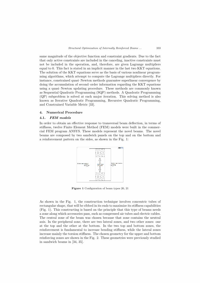
In order to obtain an effective response to transversal beam deflection, in terms ofstiffness, twelve Finite Element Method (FEM) models were built in the commer-cial FEM program ANSYS. These models represent the novel beams. The novelbeams are composed by two sandwich panels on the top and on the bottom anda reinforcement pattern on the sides, as shown in the Fig. 1:

Figure 1 Configuration of beam types 20, 21

As shown in the Fig. 1, the construction technique involves concentric tubes ofrectangular shape, that will be ribbed in its ends to maximize its stiffness capabilities(Fig. 1). This constructing is based on the principle that this type of beams needsa zone along which accessories pass, such as compressed air tubes and electric cables.The central zone of the beam was chosen because that zone contains the neutralaxis. In the peripheral zone, there are two lateral zones, and two other zones: oneat the top and the other at the bottom. In the two top and bottom zones, thereinforcement is fundamental to increase bending stiffness, while the lateral zonesincrease mainly the torsion stiffness. The chosen geometry for the upper and bottomreinforcing zones are shown in the Fig. 2. These geometries were previously studiedin sandwich beams in [34, 35].


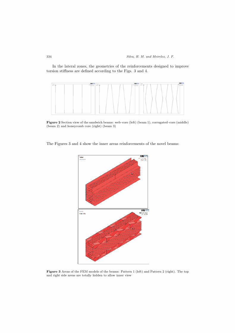
In the lateral zones, the geometries of the reinforcements designed to improvetorsion stiffness are defined according to the Figs. 3 and 4.

Figure 2 Section view of the sandwich beams: web–core (left) (beam 1), corrugated–core (middle)(beam 2) and honeycomb core (right) (beam 3)

The Figures 3 and 4 show the inner areas reinforcements of the novel beams:

Figure 3 Areas of the FEM models of the beams: Pattern 1 (left) and Pattern 2 (right). The topand right side areas are totally hidden to allow inner view


Figure 4 Areas of the FEM models of the beams: Pattern 3 (top) and Pattern 4 (bottom). Thetop and right side areas are totally hidden to allow inner view

The Fig. 5 shows an additional internal reinforcement on one of the beams, namedtransversal reinforcements. These transversal reinforcements are used in order toevaluate its influence on the improvement of the part’s stiffness. In this work, thebeams can be of two types: A and B. The beams A don’t have the transversalreinforcements that are along the beam’s flange, while all the beams B have them.The models of the Fig. 3 and 4 are of the A type, while the model represented onthe Fig. 5 is of the B type.

The results obtained in this work are in relation to a simple hollow–box beam,designated by Hollow Solid section, and abbreviated HSS with similar dimensions,but with a thickness of 2 mm, and without the internal reinforcements, as shown inthe Fig. 6.

The HSS beams (Fig. 6), were studied using the same conditions as on the sand-wich beams. These conditions and geometries, originally presented by (Silva andMeireles 2015; Silva and Meireles -), may have their mechanical behavior improvedby the use of optimization. For the FEM modelling, the used element was SHELL63(Shell Elastic 4 nodes). The elements are free quadrilateral elements with a meanlength of 0,0025 m. A mesh sensitivity analysis on the exact same geometries wasalready done by [20, 21].


Figure 5 Internal reinforcements on beam 3 pattern 3 [20, 21]

Figure 6 Areas of the FEM model representing the HSS or simple beam

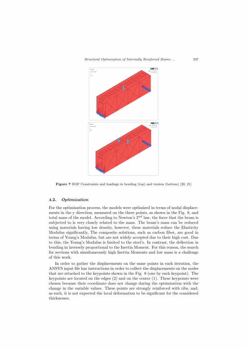
The beam was constrained in the lines of the extremities (z = 0 and z = 1), beingthe support type simply supported at its ends, as shown in Fig. 7. Concentratedloads were used by simplification in order to simulate the action of bending andtorsion. Bending was applied by one concentrated load of 1500 N, on the center ofthe top face, as shown in the Fig. 7 (top). Torsion is applied by means of a binaryload of 2000 N, as in Fig. 7 (bottom). The same load intensities were alreadyapplied to similar models by [20, 21].


Figure 7 DOF Constraints and loadings in bending (top) and torsion (bottom) [20, 21]

4.2. Optimization

For the optimization process, the models were optimized in terms of nodal displace-ments in the y direction, measured on the three points, as shown in the Fig. 8, andtotal mass of the model. According to Newton’s 2nd law, the force that the beam issubjected to is very closely related to the mass. The beam’s mass can be reducedusing materials having low density, however, these materials reduce the ElasticityModulus significantly, The composite solutions, such as carbon fiber, are good interms of Young’s Modulus, but are not widely accepted due to their high cost. Dueto this, the Young’s Modulus is limited to the steel’s. In contrast, the deflection inbending in inversely proportional to the Inertia Moment. For this reason, the searchfor sections with simultaneously high Inertia Moments and low mass is a challengeof this work.

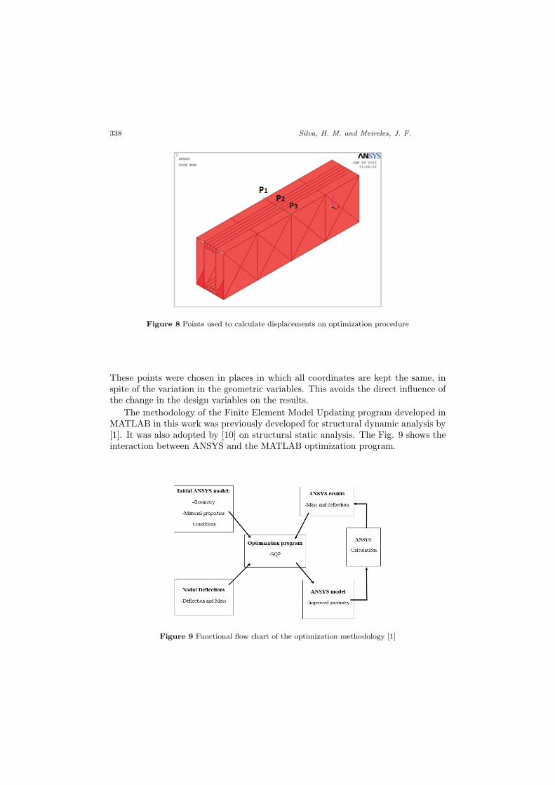
In order to gather the displacements on the same points in each iteration, theANSYS input file has instructions in order to collect the displacements on the nodesthat are attached to the keypoints shown in the Fig. 8 (one by each keypoint). Thekeypoints are located on the edges (2) and on the center (1). These keypoints werechosen because their coordinate does not change during the optimization with thechange in the variable values. These points are strongly reinforced with ribs, and,as such, it is not expected the local deformation to be significant for the consideredthicknesses.


Figure 8 Points used to calculate displacements on optimization procedure

These points were chosen in places in which all coordinates are kept the same, inspite of the variation in the geometric variables. This avoids the direct influence ofthe change in the design variables on the results.

The methodology of the Finite Element Model Updating program developed inMATLAB in this work was previously developed for structural dynamic analysis by[1]. It was also adopted by [10] on structural static analysis. The Fig. 9 shows theinteraction between ANSYS and the MATLAB optimization program.

Figure 9 Functional flow chart of the optimization methodology [1]


In this methodology, the MATLAB program works together with ANSYS. Accord-ing to ([10]): MATLAB controls the optimization by means of the MATLAB codeand ANSYS calculates the FEM results. The objective function q(x) used in thiswork is new, and the involved variables are also new (Fig. 10).

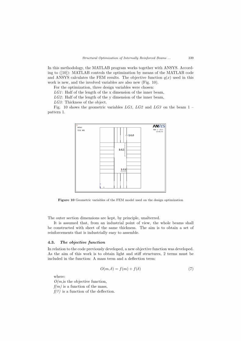
For the optimization, three design variables were chosen:LG1 : Half of the length of the x dimension of the inner beam,LG2 : Half of the length of the y dimension of the inner beam,LG3: Thickness of the object.Fig. 10 shows the geometric variables LG1, LG2 and LG3 on the beam 1 –

pattern 1.

Figure 10 Geometric variables of the FEM model used on the design optimization

The outer section dimensions are kept, by principle, unalterred.It is assumed that, from an industrial point of view, the whole beams shall

be constructed with sheet of the same thickness. The aim is to obtain a set ofreinforcements that is industrially easy to assemble.

4.3. The objective function

In relation to the code previously developed, a new objective function was developed.As the aim of this work is to obtain light and stiff structures, 2 terms must beincluded in the function: A mass term and a deflection term:

O(m, δ) = f(m) + f(δ) (7)

where:O(m,is the objective function,f(m) is a function of the mass,f(?) is a function of the deflection.


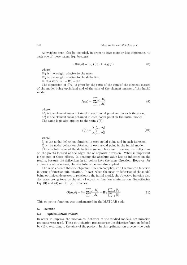
As weights must also be included, in order to give more or less importance toeach one of those terms, Eq. becomes:

O(m, δ) = W1f(m) +W2f(δ) (8)

where:W1 is the weight relative to the mass,W2 is the weight relative to the deflection.In this work W1 = W2 = 0.5.The expression of f(m) is given by the ratio of the sum of the element masses

of the model being optimized and of the sum of the element masses of the initialmodel:

f(m) =

∑nj=1 Mj∑nj=1 M

ij

(9)

where:Mj is the element mass obtained in each nodal point and in each iteration,M i

j is the element mass obtained in each nodal point in the initial model.The same logic also applies to the term f(δ):

f(δ) =

∑nj=1 |δj |∑nj=1 |δij |

(10)

where:δj is the nodal deflection obtained in each nodal point and in each iteration,δij is the nodal deflection obtained in each nodal point in the initial model.The absolute value of the deflections are sum because in torsion, the deflections

on the points located at the edges are of opposite direction. What is importantis the sum of those effects. In bending the absolute value has no influence on theresults, because the deflections in all points have the same direction. However, fora question of coherence, the absolute value was also applied.

The ratio ensures that the objective function complies with the fmincon functionin terms of function minimization. In fact, when the mass or deflection of the modelbeing optimized decreases in relation to the initial model, the objective function alsodecreases, going towards the aim of objective function minimization. SubstitutingEq. (3) and (4) on Eq. (2), it comes:

O(m, δ) = W1

∑nj=1 Mj∑nj=1 M

ij

+W2

∑nj=1 |δj |∑nj=1 |δij |

(11)

This objective function was implemented in the MATLAB code.

5. Results

5.1. Optimization results

In order to improve the mechanical behavior of the studied models, optimizationprocesses were used. These optimization processes use the objective function definedby (11), according to the aims of the project. In this optimization process, the basis


is an initial model with the same values of LG1, LG2 and LG3, as shown in the fig.10. The FEM results of the initial and optimized models are compared with the HSSbeam. The aim of the optimization routine is to minimize the objective function,to be a positive real number the closest possible to 0. The objective function valuestarts in 1 in every case, due to the fact that on the first iteration, the current modelis the same as the initial model.

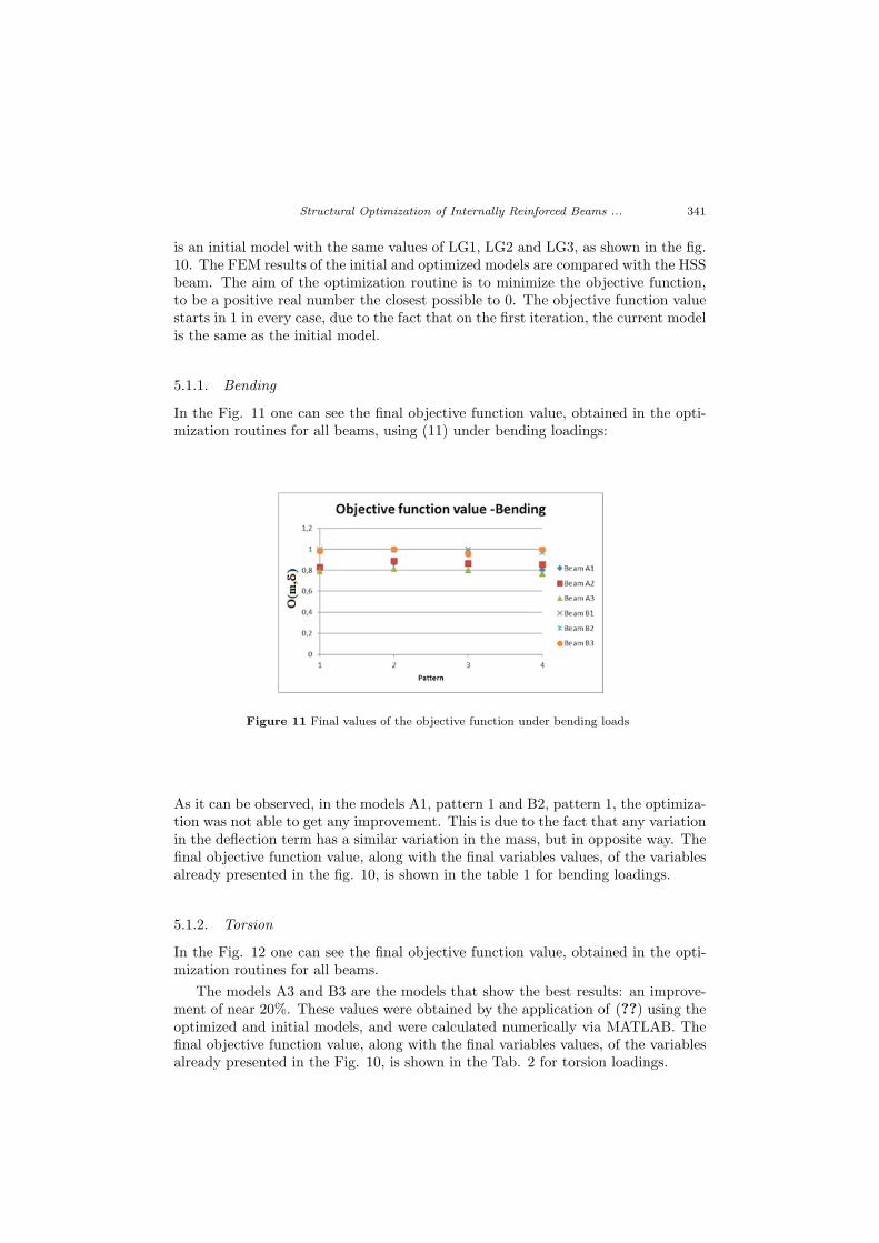
5.1.1. Bending

In the Fig. 11 one can see the final objective function value, obtained in the opti-mization routines for all beams, using (11) under bending loadings:

Figure 11 Final values of the objective function under bending loads

As it can be observed, in the models A1, pattern 1 and B2, pattern 1, the optimiza-tion was not able to get any improvement. This is due to the fact that any variationin the deflection term has a similar variation in the mass, but in opposite way. Thefinal objective function value, along with the final variables values, of the variablesalready presented in the fig. 10, is shown in the table 1 for bending loadings.

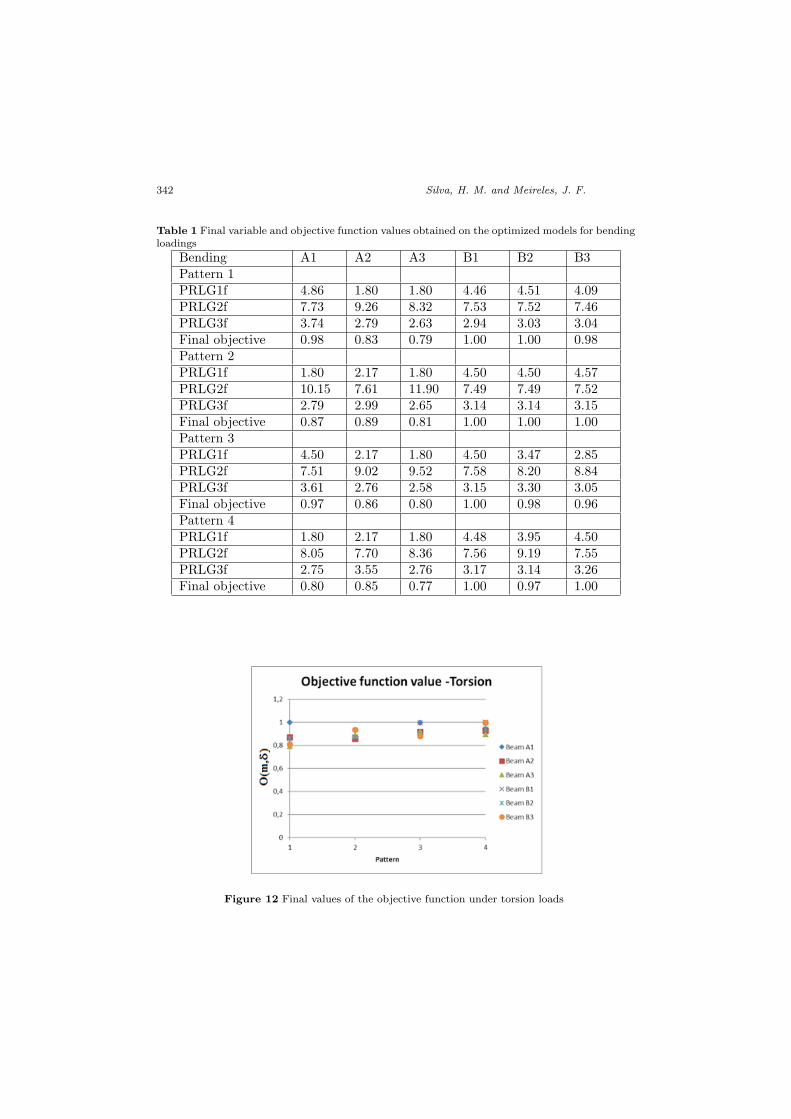
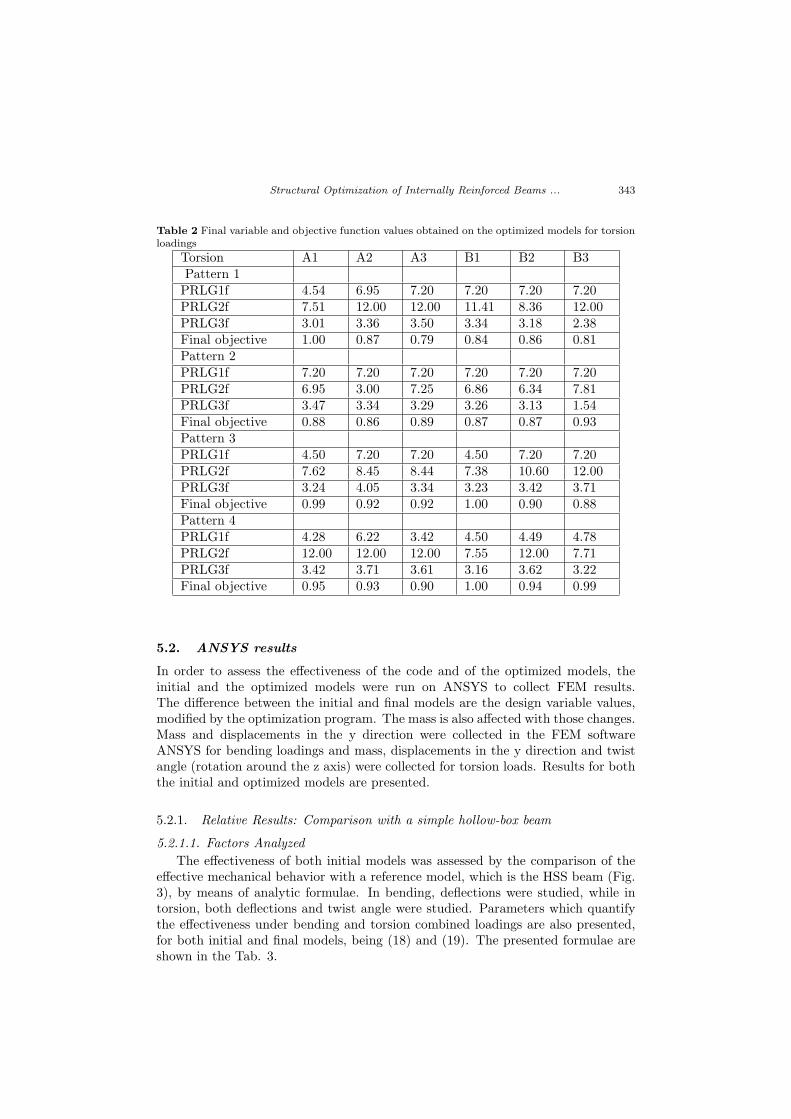
5.1.2. Torsion

In the Fig. 12 one can see the final objective function value, obtained in the opti-mization routines for all beams.

The models A3 and B3 are the models that show the best results: an improve-ment of near 20%. These values were obtained by the application of (??) using theoptimized and initial models, and were calculated numerically via MATLAB. Thefinal objective function value, along with the final variables values, of the variablesalready presented in the Fig. 10, is shown in the Tab. 2 for torsion loadings.


Table 1 Final variable and objective function values obtained on the optimized models for bendingloadings

Bending A1 A2 A3 B1 B2 B3Pattern 1PRLG1f 4.86 1.80 1.80 4.46 4.51 4.09PRLG2f 7.73 9.26 8.32 7.53 7.52 7.46PRLG3f 3.74 2.79 2.63 2.94 3.03 3.04Final objective 0.98 0.83 0.79 1.00 1.00 0.98Pattern 2PRLG1f 1.80 2.17 1.80 4.50 4.50 4.57PRLG2f 10.15 7.61 11.90 7.49 7.49 7.52PRLG3f 2.79 2.99 2.65 3.14 3.14 3.15Final objective 0.87 0.89 0.81 1.00 1.00 1.00Pattern 3PRLG1f 4.50 2.17 1.80 4.50 3.47 2.85PRLG2f 7.51 9.02 9.52 7.58 8.20 8.84PRLG3f 3.61 2.76 2.58 3.15 3.30 3.05Final objective 0.97 0.86 0.80 1.00 0.98 0.96Pattern 4PRLG1f 1.80 2.17 1.80 4.48 3.95 4.50PRLG2f 8.05 7.70 8.36 7.56 9.19 7.55PRLG3f 2.75 3.55 2.76 3.17 3.14 3.26Final objective 0.80 0.85 0.77 1.00 0.97 1.00

Figure 12 Final values of the objective function under torsion loads


Table 2 Final variable and objective function values obtained on the optimized models for torsionloadings

Torsion A1 A2 A3 B1 B2 B3Pattern 1PRLG1f 4.54 6.95 7.20 7.20 7.20 7.20PRLG2f 7.51 12.00 12.00 11.41 8.36 12.00PRLG3f 3.01 3.36 3.50 3.34 3.18 2.38Final objective 1.00 0.87 0.79 0.84 0.86 0.81Pattern 2PRLG1f 7.20 7.20 7.20 7.20 7.20 7.20PRLG2f 6.95 3.00 7.25 6.86 6.34 7.81PRLG3f 3.47 3.34 3.29 3.26 3.13 1.54Final objective 0.88 0.86 0.89 0.87 0.87 0.93Pattern 3PRLG1f 4.50 7.20 7.20 4.50 7.20 7.20PRLG2f 7.62 8.45 8.44 7.38 10.60 12.00PRLG3f 3.24 4.05 3.34 3.23 3.42 3.71Final objective 0.99 0.92 0.92 1.00 0.90 0.88Pattern 4PRLG1f 4.28 6.22 3.42 4.50 4.49 4.78PRLG2f 12.00 12.00 12.00 7.55 12.00 7.71PRLG3f 3.42 3.71 3.61 3.16 3.62 3.22Final objective 0.95 0.93 0.90 1.00 0.94 0.99

5.2. ANSYS results

In order to assess the effectiveness of the code and of the optimized models, theinitial and the optimized models were run on ANSYS to collect FEM results.The difference between the initial and final models are the design variable values,modified by the optimization program. The mass is also affected with those changes.Mass and displacements in the y direction were collected in the FEM softwareANSYS for bending loadings and mass, displacements in the y direction and twistangle (rotation around the z axis) were collected for torsion loads. Results for boththe initial and optimized models are presented.

5.2.1. Relative Results: Comparison with a simple hollow-box beam

5.2.1.1. Factors Analyzed

The effectiveness of both initial models was assessed by the comparison of theeffective mechanical behavior with a reference model, which is the HSS beam (Fig.3), by means of analytic formulae. In bending, deflections were studied, while intorsion, both deflections and twist angle were studied. Parameters which quantifythe effectiveness under bending and torsion combined loadings are also presented,for both initial and final models, being (18) and (19). The presented formulae areshown in the Tab. 3.


Table 3 Relative results: Comparison with HSS. B is the abbreviation for bending loadings, andT is the abbreviation for torsion loadings

Equation/loadings B T

Impδ∗mi(%) = [a(δy)∗m]HSS−[a(δy)∗m]i[a(δy)∗m]i

∗ 100% (14) Yes Yes

Impδ∗mf(%) =

[a(δy)∗m]HSS−[a(δy)∗m]f[a(δy)∗m]f

∗ 100% (15) Yes Yes

Impθ∗mi(%) = [a(θ)∗m]HSS−[a(θ)∗m]i[a(θ)∗m]i

∗ 100% (16) No Yes

Impθ∗mf(%) =

[a(θ)∗m]HSS−[a(θ)∗m]f[a(θ)∗m]f

∗ 100% (17) No Yes

Impδ∗mitotal(%) =[(

[a(δy)∗m]HSS−[a(δy)∗m]i[a(δy)∗m]i

)bend

+(

[a(δy)∗m]HSS−[a(δy)∗m]i[a(δy)∗m]i

)tors

](18)

Yes

Impδ∗mf total(%) =[(


)bend

+(


)tors

](19)

Yes

where:[a(δy)∗m]HSS is the global maximum y deflection as measured on the two points

multiplied by the total mass of the model for the reference model (HSS),[a(δy) ∗m]i is the global maximum y deflection as measured on the two points

multiplied by the total mass of the model for the initial models,[a(δy) ∗m]f is the global maximum y deflection as measured on the two points

multiplied by the total mass of the model for the final models,[a(θ) ∗m]HSS is the global maximum twist angle as measured on the two points

multiplied by the total mass of the model for the reference model (HSS),[a(θ) ∗ m]i is the global maximum twist angle as measured on the two points

multiplied by the total mass of the model for the initial models,[a(θ) ∗ m]f is the global maximum twist angle as measured on the two points

multiplied by the total mass of the model for the final models.

5.2.1.2. Results Analysis

In order to compare the relative effectiveness of the solutions with the ultimate aimto reach the best solution, the formulae of the table 3 were applied analytically tothe results collected from the models in ANSYS. In the Fig. 13 , one can see theeffective mechanical behavior results under bending loadings in comparison with amodel of reference for all beams using (14).

According to the results shown in the Fig. 13, one can see that the best modelsare the models B1, B2 and B3 having the pattern 4, with improvements rangingfrom 7000% to near 8500%. There is an improvement for all models, although themodel B1, pattern 4 shows the best results, showing an improvement of near 8500%.The worst models are the models A1, A2 and A3, which are worse than any of theB beams for every pattern.

In the Fig. 14, one can see the effective mechanical behavior of the optimizedmodels in comparison with the simple hollow-box beam under bending loadings


Figure 13 Effective mechanical behavior of the initial models in comparison with the simplehollow-box beam under bending loadings for beams without transversal reinforcements

Figure 14 Effective mechanical behavior of the optimized models in comparison with the simplehollow-box beam under bending loadings for beams without transversal reinforcements

According to the results shown in the Fig. 14, one can see that the best modelsare the B models having the pattern 4, with improvements ranging from 7000% to8500%. The A beams show an improvement of near 6000%. According to the fig.14, the best models are the models of the pattern 4 with improvements rangingfrom 7000% to near 8500%, approximately. For both A and B models, there is animprovement for all models.

In the fig. 15, one can see the effective mechanical behavior results under torsionloadings in comparison with a model of reference for all beams, using (??).

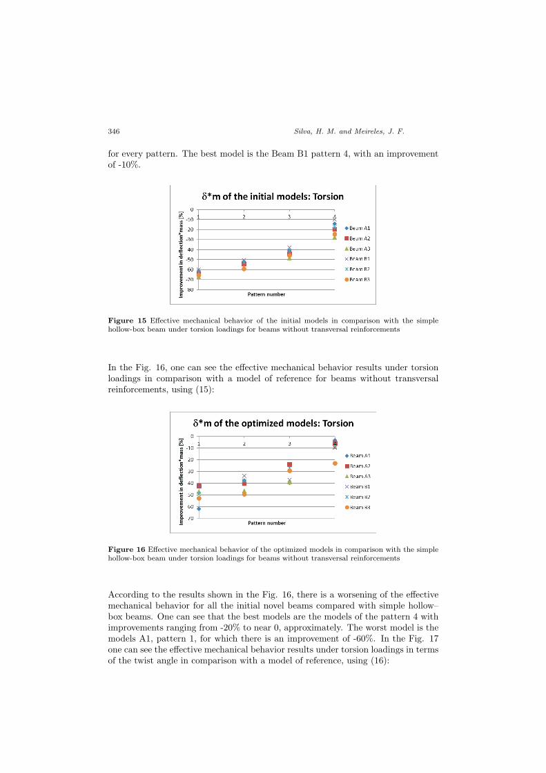
According to the results shown in the Ffig. 15, there is a worsening for allmodels, although the pattern 4 shows the best results for all beams in comparisonwith the other patterns. The worst models are all the models of the pattern 1, withan improvement ranging from -70% to -60%. The beam B1 shows the best results


for every pattern. The best model is the Beam B1 pattern 4, with an improvementof -10%.

Figure 15 Effective mechanical behavior of the initial models in comparison with the simplehollow-box beam under torsion loadings for beams without transversal reinforcements

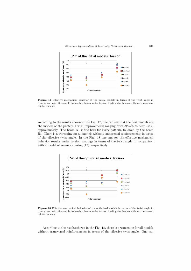
In the Fig. 16, one can see the effective mechanical behavior results under torsionloadings in comparison with a model of reference for beams without transversalreinforcements, using (15):

Figure 16 Effective mechanical behavior of the optimized models in comparison with the simplehollow-box beam under torsion loadings for beams without transversal reinforcements

According to the results shown in the Fig. 16, there is a worsening of the effectivemechanical behavior for all the initial novel beams compared with simple hollow–box beams. One can see that the best models are the models of the pattern 4 withimprovements ranging from -20% to near 0, approximately. The worst model is themodels A1, pattern 1, for which there is an improvement of -60%. In the Fig. 17one can see the effective mechanical behavior results under torsion loadings in termsof the twist angle in comparison with a model of reference, using (16):


Figure 17 Effective mechanical behavior of the initial models in terms of the twist angle incomparison with the simple hollow-box beam under torsion loadings for beams without transversalreinforcements

According to the results shown in the Fig. 17, one can see that the best models arethe models of the pattern 4 with improvements ranging from -98.5% to near -98.2,approximately. The beam A1 is the best for every pattern, followed by the beamB1. There is a worsening for all models without transversal reinforcements in termsof the effective twist angle. In the Fig. 18 one can see the effective mechanicalbehavior results under torsion loadings in terms of the twist angle in comparisonwith a model of reference, using (17), respectively.

Figure 18 Effective mechanical behavior of the optimized models in terms of the twist angle incomparison with the simple hollow-box beam under torsion loadings for beams without transversalreinforcements

According to the results shown in the Fig. 18, there is a worsening for all modelswithout transversal reinforcements in terms of the effective twist angle. One can


see that the best models are the models of the pattern 4 with improvements rangingfrom near -98.4% to near -97.8, approximately. Of those models, one can see thatthe best model is the Beam A2 pattern 4 with a worsening of -97.8%, approximately.

In the Fig. 19, one can see the effective mechanical behavior results in terms oftotal improvement in comparison with a model of reference, using (??).

Figure 19 Total improvement of the initial models in terms of deflection in comparison withthe simple hollow-box beam considering both bending and torsion loadings for beams withouttransversal reinforcements

According to the Fig. 19, the best models are the B models of the pattern 4 withimprovements ranging from 7000% to near 8000%, approximately. One can see thatthe B models are better than the A models for every pattern. The results for theA beams vary from between near 2000% for every A beam, for the patterns 1,2and 3, to near 3000% for the pattern 4. In the fig. 23, one can see the effectivemechanical behavior results in terms of total improvement in comparison with amodel of reference, using (19), respectively.

Figure 20 Total improvement of the optimized models in terms of deflection in comparison withthe simple hollow-box beam considering both bending and torsion loadings for beams withouttransversal reinforcements


According to the Fig. 20, the best models are the B models of the pattern 4 withimprovements ranging from 7000% to near 8000%, approximately. For all patterns,the B beams perform better than the A beams.

6. Results discussion

The results obtained under bending loadings prove that the developed beams arevery effective under bending loadings. In fact, the sandwich reinforcements at thetop and at the bottom dramatically increase the resistance moment and the inertiamoment, while keeping the mass to a minimum. Under torsion loadings, the beamsdo not perform so well under the developed parameters due to the fact that thehighest reinforcement density is located at the top and at the bottom. The rein-forcement on the sides are more important for torsion, due to the fact that theyare oriented transversally and diagonally, and, therefore, have an influence on theinertia moment under torsion loadings. The optimization procedure is shown to bevery effective in optimizing most of the models, improving its effective mechanicalbehavior, both in bending and torsion loadings. The developed parameters (Tab.3) allowed to evaluate the effectiveness of the optimization code and of the objectivefunction, and also the evaluation of the effectiveness of the mechanical behavior ofboth initial and optimized models in terms of the Finite Element Method resultsobtained in ANSYS MECHANICAL APDL. The developed beams are very inter-esting for applications where bending loadings act isolate or coupled with torsion,in the case that the torsional component of the loadings have a less important effectthan the bending component.

7. Conclusions

The following conclusions can be drawn from this work:

– The objective function developed is effective in improving the mechanicalbehavior of the FEM models while keeping the mass to a minimum both in torsionand in bending loadings. This can be proved by the results comparison betweeninitial and optimized models.

– The models with transversal ribs are shown to be quite more effective thanthe ones without in terms of the total improvement.

– The best beam without transversal reinforcements after optimization is theBeam A1, pattern 4, with improvement close to 8500%.

– The best beam with transversal reinforcements is also the beam 1, Pattern 4.

– The novel beams are very effective in bending, while not so much under torsionloadings. The behavior under torsion loadings may be in reality better than inthis study, due to the fact that one is comparing results on the point of loadingapplication and that loading point is weaker in the novel beams than in the simplebeams. For distributed loads, as it may happen in reality, it is expected that theload distribution will reduce the effect of the concentrated load.

– The studied beams can, therefore, be interesting for industrial applications,mainly in applications with mobile parts, where there is the need of light and stiffbeams.


References

[1] De Meireles, J. F.: Analise dinamica de estruturas por modelos de elementos finitosidentificados experimentalmente. PhD Thesis, University of Minho, 2007.

[2] Bin, X., Nan , C. and Huajun, C.: An integrated method of multi-objectiveoptimi-zation for complex mechanical structure, Advances in Engineering Software41, 277–285, 2010.

[3] Brill, E. D., Chang, S-Y and Hopkins, L. D.: Modeling to generate alternatives:The HSJ approach and an illustration using a problem in land use planning. ManageSci, 28:221, 1982.

[4] Brill, E. D., Flach, J.M., Hopkins, L. D. and Ranjithan, S.: MGA: A decisionsupport system for complex, incompletely defined problems. IEEE Trans Syst ManCybern, 20:745, 1990.

[5] Baugh, J. W., Caldwell, S. and Brill, E. D.: A mathematical programmingapproach for generating alternatives in discrete structural optimization, Eng Optim,28:1, 1997.

[6] Zarate, B.A., Caicedo, J.M.: Finite element model updating: Multiple alterna-tives. Elsevier, Engineering Structures, 30, 3724–3730, 2008.

[7] Bakir, P. G., Reynders, E., and De Roeck, G.: An improved finite elementmodel updating method by the global optimization technique Coupled Local Mini-mizers, Computers and Structures, 86, 1339–1352, 2008.

[8] Kalanta, S., Atkociunas, J. and Venskus, A.. Discrete optimization problemsof the steel bar structures. Engineering Structures, 31, 1298–1304, 2009.

[9] Silva, H. M., De Meireles, J. F.. Determination of the Material/Geometry of thesection most adequate for a static loaded beam subjected to a combination of bendingand torsion. Materials Science Forum 730-732, 507–512, 2013.

[10] Silva, H. M.:Determination of the Material/Geometry of the section most adequatefor a static loaded beam subjected to a combination of bending and torsion. MScThesis, University of Minho, 2011.

[11] Lee, J., Kim, S-M, Park, H-S and Woo, B-H.: Optimum design of cold-formedsteel channel beams using micro Genetic Algorithm, Engineering Structures, 27, 17–24, 2005.

[12] Liu, H., Igusa, T. and Schafer, B.W.: Knowledge-based global optimization ofcold-formed steel columns, Thin-Walled Structures, 42, 785–801, 2004.

[13] Magnucka-blandzi, E., Magnucki, K..: Buckling and optimal design of cold-formed thin-walled beams: Review of selected problems, Thin-Walled Structures, 49,554–561, 2011.

[14] Leng, J., Guest, J.K. and Schafer, B.W.: Shape optimization of cold-formedsteel columns, Thin-Walled Structures, 49, 1492–1503, 2011.

[15] Theofanous, M., Chan, T.M. and Gardner, L..: Structural response of stainlesssteel oval hollow section compression members, Engineering Structures, 31, 922–934,2009.

[16] Lagaros, N.D., Psarras, L.D., Papadrakakis, M. and Panagiotou, G..: Op-timum de-sign of steel structures with web openings, Engineering Structures, 30,2528–2537, 2008.

[17] Tsavdaridis, K.D. and D’Mello, C..: Optimisation of novel elliptically-based webopening shapes of perforated steel beams, Journal of Constructional Steel Research,76, 39–53, 2012.


[18] McKinstray, R., Lim, J.B.P., Tanyimboh, T.T., Phan D.T. and Sha, W..:Optimal design of long-span steel portal frames using fabricated beams, Journal ofConstructional Steel Research, 104, 104–114, 2015.

[19] Tran, T., Li, L-Y.: Global optimization of cold-formed steel channel sections. Thin-Walled Structures, 44, 399–406, 2006.

[20] Silva, H. M., De Meireles, J. F..: Feasibility of internally reinforced thin-walledbeams for industrial applications, Applied Mechanics and Materials, 775, 119–124,2015.

[21] Silva, H. M., De Meireles, J. F.: - Feasibility of Internally Stiffened Thin-WalledBeams for Industrial Applications [submitted].

[22] Schittkowski, K..: NLQPL: A FORTRAN-Subroutine Solving Constrained. Non-linear Programming Problems, Annals of Operations Research, 5, 485-500, 1985, inhttp://wwwmathworks.com.

[23] Biggs, M. C..: Constrained Minimization Using Recursive Quadratic Pro-gramming,Towards Global Optimization. LCW Dixon and GP Szergo, eds North-Holland 341–349, in http://wwwmathworkscom, 1975.

[24] Han, S. P.: A Globally Convergent Method for Nonlinear Programming, Journal ofOptimization Theory and Applications, 22:297, 1977, in http://www.mathworks.com.

[25] Powell, M. J. D.: The Convergence of Variable Metric Methods for NonlinearlyConstrained Optimization Calculations, Nonlinear Programming 3, OL Mangasarian,RR Meyer and SM Robinson, eds, Academic Press, in http://www.mathworks.com,1978.

[26] Powell, M. J. D.: A Fast Algorithm for Nonlinearly Constrained OptimizationCalculations, Numerical Analysis, GA Watson ed, Lecture Notes in Mathematics,Springer Verlag, 630, in http://wwwmathworks.com, 1978.

[27] Fletcher, R.: Practical Methods of Optimization, John Wiley and Sons, inhttp://www.mathworks.com, 1987.

[28] Gill, P. E., Murray, W. and Wright, M. H..: Practical Optimization, London,Academic Press, in http://www.mathworks.com, 1981.

[29] Powell, M.J.D.: Variable Metric Methods for Constrained Optimization. Mathe-matical Programming: The State of the Art, A Bachem, M Grotschel and B Korte,eds Springer Verlag, 288–311, in http://wwwmathworks.com, 1983.

[30] Hock, W., Schittkowski, K. A..: Comparative Performance Evaluation of 27 Non-linear Programming Codes, Computing 30:335, in http://www.mathworks.com 1983.

[31] http://www.mathworks.com/help/optim/ug/constrained-nonlinear-optimization-algorithms.html. Accessed 11 March 2016.

[32] http://www.mathworks.com/help/optim/ug/fmincon.html. Accessed 2016.

[33] http://www.mathworks.com/help/optim/ug/optimization-theory-overview.html#bqa jby. Accessed 2016.

[34] Silva, H.M., De Meireles, J.F..: Effective Mechanical Behavior of Sandwich Beamsunder Uncoupled Bending and Torsion Loadings, Applied Mechanics and Materials,590, 58–62, 2014,.

[35] Silva, H. M., De Meireles, J. F.: Effective Stiffness Behavior of Sandwich Beamsunder Uncoupled Bending and Torsion Loadings, 852, b, 469–475, 2016.

structural optimization of internally reinforced beams ... · the finite element method-fem...

Documents