STRUCTURAL HEALTH MONITORING FOR

BRIDGES USING ADVANCED DATA ANALYSIS FOR

PROCESS NON-LINEARITY AND NON-

STATIONARITY

By

ERMIAS BIRU

Bachelor of Science in Industrial Engineering

Bahir Dar University

Bahir Dar, Ethiopia

2004

Submitted to the Faculty of the

Graduate College of the

Oklahoma State University

in partial fulfillment of

the requirements for

the Degree of

MASTER OF SCIENCE

December, 2010

ii

STRUCTURAL HEALTH MONITORING FOR

BRIDGES USING ADVANCED DATA ANALYSIS FOR

PROCESS NON-LINEARITY AND NON-

STATIONARITY

Thesis Approved:

Dr. Zhenyu (James) Kong

Thesis Adviser

Dr. Tieming Liu

Dr. Tyler Ley

Dr. Mark E. Payton

Dean of the Graduate College

iii

ACKNOWLEDGMENTS

I would like to express my deepest appreciation to my advisor, Dr. Zhenyu

(James) Kong, for his continuous support, patience and excellent guidance throughout my

study. I learned many important lessons from him and he is always there to listen, advise

and motivate me.

I would like to thank Dr. Tieming Liu and Dr. Tyler Ley for serving on my thesis

committee as well as for their valuable input throughout my study and during my thesis

defense. I am grateful to Dr. Ley for his support in providing the data used for analysis.

I am also grateful for the support and guidance that I had from my senior and

doctoral students Mr. Asil Oztekin and Mr. Omer Beyca. I am also thankful to Mr.

Mahmoud Z. Mistarihi for his suggestion and help in organizing the document.

This thesis would not have been possible without the help of my parents Mrs.

Aberu Abtew and Mr. Belay Biru who encouraged me from the initial to the final level of

my study. I am also grateful to the support I had from my sisters and brothers.

Finally, I offer my regards to Mr. Getachew Tsegay, Mr. Kumlachew

Woldesenbet, and others who supported me in any respect during my study.

iv

TABLE OF CONTENTS

Chapter Page

I. INTRODUCTION ......................................................................................................1

1.1 Research Motivation ..........................................................................................1

1.2 Problem Statement .............................................................................................2

1.3 Research Objectives ...........................................................................................3

1.4 Research Methodologies ....................................................................................4

1.5 Thesis Organization ...........................................................................................4

II. REVIEW OF LITERATURE....................................................................................6

2.1 Introduction to SHM .........................................................................................6

2.2 Phases of SHM ..................................................................................................6

2.2.1 Operational Evaluation ............................................................................7

2.2.2 Data Acquisition .......................................................................................9

2.2.2.1 Excitation Methods ........................................................................10

2.2.2.2 Sensor Application in SHM ...........................................................11

2.2.3 Feature Extraction ...................................................................................12

2.2.3.1 ARIMA Model Families ................................................................13

2.2.3.2 Modal Parameters ..........................................................................14

2.2.3.3 Energy Distribution ........................................................................15

2.2.4 Statistical Model Development ...............................................................16

2.3 SHM Data Processing and Statistical Application...........................................18

2.3.1 SHM-based on Time Series Analysis .....................................................18

2.3.2 SHM-based on Frequency Domain Analysis ..........................................20

III. PROPOSED METHODOLOGY AND CASE STUDY ........................................24

3.1 Time Series Modeling ......................................................................................24

3.2 Frequency Domain Analysis ............................................................................27

3.2.1 Fourier Transform ...................................................................................29

3.2.2 Wavelet Transform .................................................................................34

3.2.3 Hilbert Huang Transform and Empirical Mode Decomposition ............38

3.2.3 1 Hilbert Huang Transform (HHT) ...................................................38

v

Chapter Page

3.2.3.2 Empirical Mode Decomposition (EMD) .......................................42

3.2.4 Comparison of Fourier, Wavelet and Hilbert Transform........................47

IV. IMPLEMENTATION OF PROPOSED METHODOLOGY ...............................50

4.1 Data Sources for Analysis ................................................................................50

4.1.1 Data Source from A Bridge ....................................................................50

4.1.2 Data Source from Simulation Data .........................................................51

4.2 Frequency Domain Analysis of Simulation Data ............................................53

4.2.1 Fourier Transform of Simulation Data ...................................................61

4.2.2 Wavelet Analysis of Simulation Data .....................................................62

4.2.3 Hilbert-Huang Application to Simulation Data ......................................63

4.3 Statistical Analysis of Bridge Data ..................................................................73

4.4 Time Series Modeling of Bridge Data .............................................................79

V. SUMMARY AND CONCLUSION.......................................................................89

5.1 Summary of Findings .......................................................................................89

5.2 Future Work .....................................................................................................91

REFERENCES ............................................................................................................93

vi

LIST OF TABLES

Table Page

Table 3.1 Relationship between time resolution and frequency resolution in STFT ...34

Table 3.2 Comparison between the different frequency domain analysis

methodologies .............................................................................................49

Table 4.1 Damage patterns and their description considered in the Matlab

program. ......................................................................................................53

Table 4.2 Different damage scenarios considered .......................................................55

Table 4.3 Fourier transform output values for the four damage cases. ........................61

Table 4.4 Success rate of the mean and variance test in rejecting the null

hypothesis ....................................................................................................70

Table 4.5 Success rate of the mean and variance test in rejecting the null

hypothesis from IMF-1 to IMF-4 ................................................................71

Table 4.6 Damage patterns for case-5..........................................................................71

Table 4.7 Correlation coefficient among the 4-sensors. ..............................................75

Table 4.8 Summary of correlation coefficient values. .................................................75

Table 4.9 Rate of increase of deformation for 4 sensors from column-1 . ..................79

Table 4.10 Sample extended autocorrelation function (EACF) for diff(y) ................84

vii

LIST OF FIGURES

Figure Page

Fig. 2.1 Basic steps in SHM system. .............................................................................7

Fig. 2.2 Application of strain gauges for SHM. ...........................................................12

Fig. 3.1 Flow chart showing the applicability of frequency domain approaches. .......28

Fig. 3.2 Time series plot of signal x(t). ........................................................................30

Fig. 3.3 Fourier transform of signal x(t).. ....................................................................30

Fig. 3.4 Time series plot of signal y(t). ........................................................................31

Fig. 3.5 Fourier transform of signal y(t). .....................................................................32

Fig. 3.6 The wavelet transforms process.. ...................................................................35

Fig. 3.7 Relationship between scale and frequency in wavelet transform. ..................36

Fig. 3.8 Translation of a mother wavelet along a signal for a s=1. ..............................36

Fig. 3.9 Translation of a mother wavelet along a signal for a s=5. ..............................37

Fig. 3.10 Time series plots of signals of sin x +α, for α =0, 0.5, 1.5. ..........................40

Fig. 3.11 Hilbert transform of sin x+ α for α =0, 0.5, 1.5. ...........................................41

Fig. 3.12 Phase angle of sin x+ α for α =0, 0.5, 1.5. ....................................................41

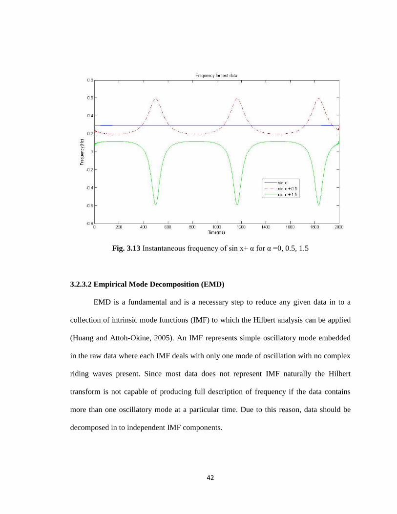
Fig. 3.13 Instantaneous frequency of sin x+ α for α =0, 0.5, 1.5. ................................42

Fig. 3.14(a) The cubic spline upper and the lower envelopes and their mean h1. .......44

Fig. 3.14(b) Comparison between data x(t) and h1. ....................................................44

Fig. 3.14(c) Repeat the sifting process using h1 as data. .............................................45

Fig. 3.15 Flow chart showing the steps in EMD..........................................................46

Fig. 3.16 Time series plot of a chrip signal..................................................................47

Fig. 3.17 Fourier transform of chrip signal. .................................................................47

Fig. 3.18 Continuous wavelet transform of the chrip signal. .......................................48

viii

Figure Page

Fig. 3.19 Instantaneous frequency plot of the chrip signal.. ........................................48

Fig. 4.1 Supporting column of the bridge.. ..................................................................51

Fig. 4.2 Picture and 3D model showing the bench mark problem building. ...............52

Fig. 4.3 The six damage patterns defined by the Benchmark problem........................54

Fig. 4.4 Time series plot of the damage scenarios considered (case1-case 4).. ...........56

Fig. 4.5 Fourier transform of the four cases (case1-case 4).. .......................................57

Fig. 4.6 Wavelet transform (2D) of the four cases (case1-case 4).. .............................58

Fig.4.7(a) 3D-wavelet transform for case-1. ................................................................59

Fig. 4.7(b) 3D-wavelet transform for case-2. ..............................................................59

Fig. 4.7(c) 3D-wavelet transform for case-3. ...............................................................60

Fig. 4.7(d) 3D-wavelet transform for case-4. ..............................................................60

Fig. 4.8 Comparison of frequency from Fourier transform for the four damage

cases.. ..............................................................................................................62

Fig. 4.9 IMF components of case-1 after EMD of the raw signal.. .............................64

Fig.4.10 Instantaneous frequency plot for (case-1-case-4) from the 1st IMF of

each case. ......................................................................................................65

Fig. 4.11 Two sample (case1&case2) Variance test.. ..................................................68

Fig. 4.12 Two sample (case1&case2) Mean test.. .......................................................68

Fig. 4.13 Two sample (case1&case3) Variance test.. ..................................................68

Fig. 4.14 Two sample (case1&case3) Mean test.. .......................................................69

Fig. 4.15 Two sample (case1&case4) Variance test.. ..................................................69

Fig. 4.16 Two sample (case1&case4) Mean test. ........................................................69

Fig. 4.17 Two sample (case1&case5) Mean test. ........................................................73

Fig. 4.18 Comparison of strain measurement from the 4 sensors of column-1. ..........74

Fig. 4.19 Matrix plot showing the correlation among the 4-sensors.. .........................76

Fig. 4.20 Time series plot for the temperature readings at the 4-sensors from

Column-1.. ....................................................................................................76

Fig. 4.21 Relationship between temperature and deformation recordings. .................78

Fig. 4.22 Rate of increment of deformation for year 1, year 2 and year 3).. ...............78

ix

Fig. 4.23 Time series plot for sensor-4 with different time period.. ............................80

Fig.4.24 Time series plot for sensor-4 (3-years). .........................................................81

Fig.4.25 Box-Cox plot for sensor-4.. ...........................................................................82

Fig.4.26 Time series plot for diff(y).. ..........................................................................83

Fig.4.27 ACF and PACF plot for diff(y). ....................................................................83

Fig. 4.28 R-output for parameter estimation for model orders c= (3, 1,2) c=(1,1,4)

and c=(2,1,2). ................................................................................................85

Fig.4.29 Diagnostic plot for the fitted ARIMA c= (2,1,2) model.. ..............................87

Fig.4.30 Normality test for the residuals.. ...................................................................88

1

CHAPTER I

INTRODUCTION

1.1 Research Motivation

There are more than 600,000 highway bridges in the united states ASCE (2009).

Guidelines by the AASHTO (2007) suggest that the expected service life of a bridge to

be a minimum of 75 years. The majority of bridges currently in use were built after

1945. However, significant environmental damage requiring repair typically occurs

before the average bridge reaches mid-life. In 2005, the ASCE estimated that it would

take $188 billion over the next 20 years to eliminate bridge deficiencies in the United

States (ASCE, 2005). The cost of delaying these repairs is significant as delay leads to

increases in road user costs, material, and construction costs.

It is possible that the condition or health of these bridges could be effectively

monitored by using sensors. Using sensor information, more informed repair and

maintenance decisions could be made. Furthermore, these sensors may be able to give the

local state Departments of Transportations (DOTs) information about when a bridge is

nearing the end of its usable life. While this could be a useful tool, it is not currently cost-

effective to monitor the health of common structures due to the high cost of sensors,

2

installation of these sensors and, ultimately, the monitoring of the sensor system.

However, it has been found to be cost-effective by several DOTs to use structural health

monitoring (SHM) on major “lifeline” or critical structures. These structures are of such

great importance to the public that they must remain open and be maintained to last as

long as possible.

According to the FHWA and US DOT (2009) report there are more than 600,000

bridges in the United States and 11.8% of the bridges are structurally defective and

13.01% are functionally obsolete and more than $17 billion is needed to improve the

current condition of bridges. Visual inspection is the primarily method used to evaluate

the condition of these bridges. SHM can help the decision making process of

classification of condition of bridges by assessing the internal condition of the bridge

structures where it would be inaccessible or uneconomical by the visual inspection

approach. The consequence of ineffective inspection of bridges can be very severe. The

collapse of the I-35W Mississippi River Bridge on August 1, 2007 in Minneapolis caused

a loss of13 lives and the replacement cost for the bridge was about $234 million. Other

costs are incurred as a result of increased commute times, loss of business from lack of

local access, and lost revenue from the blockage of a major river shipping channel.

According to the (NTSB, 2007) report the bridge is collapsed due to design defects and

excess load at the time of the collapse.

1.2 Problem Statement

Components that directly affect the performance of the bridge must be

periodically inspected or monitored. Currently, visual inspection is the primary method

3

used to evaluate the condition of most highway bridges. Inspectors periodically visit each

bridge to assess its condition. This type of inspection is highly dependent upon the

individual inspectors‟ experiences. Even for experienced inspectors, it is difficult to

detect corrosion and crack development inside of structural elements, and almost

impossible to realize the resulting changes in deflections of the structure due to local

changes in stiffness. Moreover visual inspection is labor intensive and costly.

1.3 Research Objectives

Due to the shortcomings of traditional inspection methods and advancement in

sensor technology and wireless data transmission, researchers have turned their attention

to SHM in recent years. SHM is generally a type of non-destructive inspection (NDI)

which allows the examination or testing of an object or material without affecting the

operational life or causing damage. The ultimate goal of the research in this thesis is

application of data processing methodologies and statistical techniques for response data

acquired from sensors for the purpose of SHM. The objectives of this research include:

(i) Time series modeling and spectral analysis of data gathered from a normal

working state and damaged state to validate the proposed signal processing

tools.

(ii) Application of statistical tools to support the proposed signal processing

approaches to be able to decide when damage occurs to a structure.

(iii) Prediction or forecasting of damage indicator parameters based on past

recorded values.

4

1.4 Research Methodology

Damage to a civil structure can be detected by processing or analyzing response

data obtained from sensors installed on the structure such as a bridge. The premise

behind these response data analysis methodologies is that when damage occurs to a

structure, it induces changes in the structural properties which results in loss of stiffness

or a change in energy dissipations of the structure. These changes in turn will alter the

measured dynamic response of the structure.

To detect the incurred damage, time series modeling and spectral analysis

approaches are utilized in this research. High volume data from a functional bridge is

analyzed in a step by step approach from a time series perspective. Frequency domain

approaches which include Fourier transform, wavelet analysis and Hilbert transform were

also applied on a simulation data of a benchmark problem. Comparison of the

effectiveness and sensitivity of the methodologies was also the subject of this research.

The main feature extraction or damage indicator parameter approaches used in this study

were frequency changes in the spectral analysis tools while time series and statistical

analysis tools were applied to detect the changes in the amount of deformation developed

on a supporting column of a bridge.

1.5 Thesis Organization

Background and a detailed review of recent development of SHM are discussed in

chapter 2. Prior studies conducted on feature extraction and signal processing for the

purpose of SHM are also revised in this chapter. In chapter 3 proposed methodologies of

data processing approaches and case studies to show the applicability of the methods are

5

described in detail. Chapter 4 presents the application of the proposed methodologies for

data obtained from a currently working bridge and a benchmark simulation. Presented in

chapter 5 are the conclusion and summary of the research work together with the

recommendations for future study in this area.

6

CHAPTER II

LITRETURE REVIEW

2.1 Introduction to Structural Health Monitoring

According to (Sohn et al., 2003) Structural Health Monitoring (SHM) can be

defined as “the process of implementing a damage detection strategy for aerospace, civil

and mechanical engineering infrastructure”. In this context, damage is defined as

changes in the geometric or material properties of the infrastructures, which negatively

affect the normal working condition. For example, a crack that develops on a supporting

column of a bridge invokes a change in the stiffness of the column; hence it can be

considered as damage.

2.2 Phases of Structural Health Monitoring

SHM deals with the observation of structures, such as, bridges or buildings, over a

period of time; by means of response measurement data acquired from sensors, feature

extraction from the measurement system and the application of statistical tools to detect

the presence of damage.

7

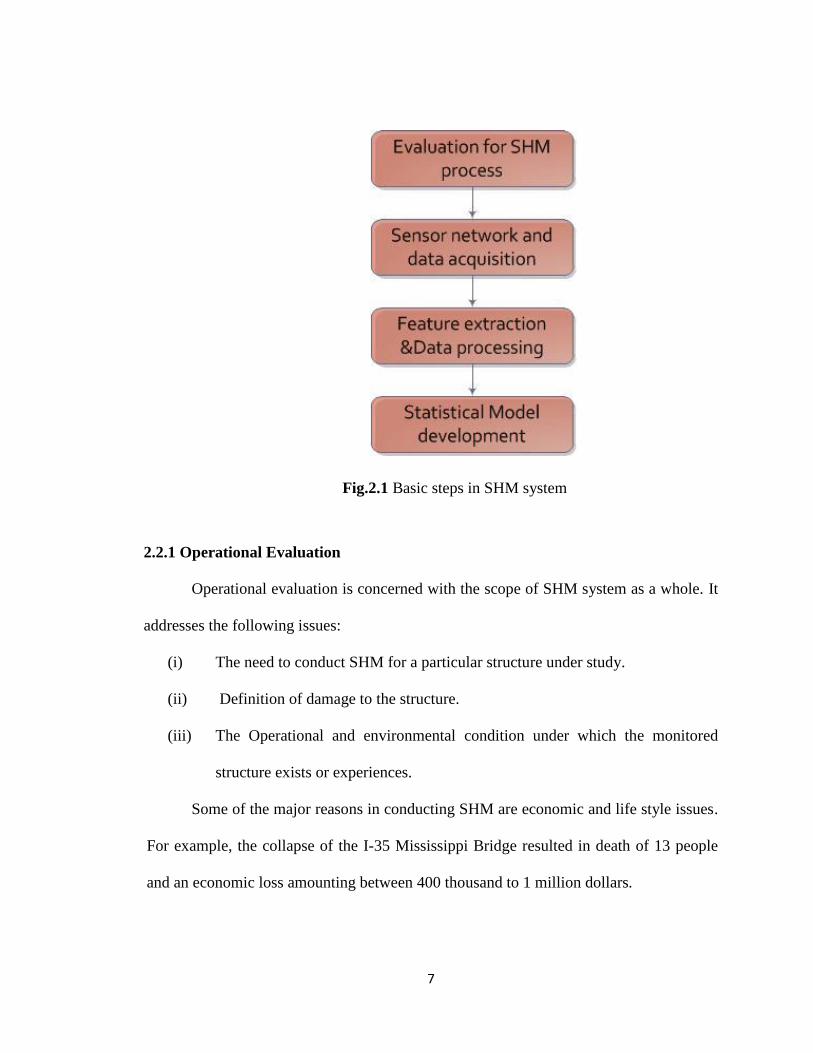
Fig.2.1 Basic steps in SHM system

2.2.1 Operational Evaluation

Operational evaluation is concerned with the scope of SHM system as a whole. It

addresses the following issues:

(i) The need to conduct SHM for a particular structure under study.

(ii) Definition of damage to the structure.

(iii) The Operational and environmental condition under which the monitored

structure exists or experiences.

Some of the major reasons in conducting SHM are economic and life style issues.

For example, the collapse of the I-35 Mississippi Bridge resulted in death of 13 people

and an economic loss amounting between 400 thousand to 1 million dollars.

8

Environmental and operational conditions should also be considered while

implementing SHM. Doebling and Farrar (1997) state that the modal analysis of

Alamosa Canyon Bridge in New Mexico depicts first mode frequency variation due to

the temperature difference recorded within 24 hours. The implication here is that,

changes in the surrounding conditions can produce a far more significant amount of

variation on measured parameters compared with the actual damage progress

experienced by the structure. Staszewki et al. (2000) discuss that ambient vibration and

temperature could affect piezoelectric sensors negatively, which is mounted on

composite plates. The delimitation in the composite plates was concealed by temperature

variability. Rohrmann et al. (1999) found that a structure‟s material properties were

altered as a result of change in temperature and this change resulted in a change in the

reaction forces from the bridge supports. The authors also formulated a mathematical

modal using regression to show the effect of temperature on the natural frequency.

Δf=a0T0+a1ΔT 2.1

As the equation shows, there is a linear relationship between temperature change and

natural frequency. According to the article by (Wong et al., 2001), the displacement

response of a bridge is the combined effect of impacts, which arise from major sources of

wind, temperature, highway, and railway. The authors further discussed the effect that

temperature has on long suspension bridges. Temperature difference could cause damage

to a bridge by forcing expansion and contraction of the bridge along the longitudinal

direction. The effect of wind and rain-wind induced vibration on the performance of a

bridge is discussed in the report by (Zuo et al., 2010).

9

2.2.2 Data Acquisition

The acquisition of data is one of the integral components of a modern SHM

system. Issues such as how often to collect the data, the type, placement and number of

sensors are also handled in this step. After the data has been produced, it is necessary to

get this information from the data acquisition system and to the user to evaluate.

Sampling and processing of signals, usually manipulated by a computer, to obtain the

desired information is referred to as Data Acquisition (DAQ).

The components of data acquisition systems include appropriate sensors that

convert any measurement parameters to electrical signals, which are acquired, displayed,

analyzed and stored on a PC by interactive control software and hardware. A general

understanding of this system and its components is essential in order to design an

efficient and useful monitoring program. Generally, there are two common data

acquisition systems, namely, the manual and computer based systems.

In a manual system, the operator visually reads the data from the read out units

and records it manually. Since this system does not need bulky equipments, it is an

economical and convenient way to collect data from a small number of sensors within a

short period of time. However, for more general applications, a computer based

acquisition system must be used. The components of this data acquisition system are

signal conditioners, one or more data acquisition boards, and a computer.

10

2.2.2.1 Excitation Methods

Prior to obtaining the data, there should be some sort of excitation method applied

on the structure of interest. Generally, the excitation methods that we use to vibrate or set

a structure in to motion can be categorized in to forced excitation and ambient excitation.

Forced excitation: in this category, a number of different excitations methods are

applied. Some of the most commonly used are: actuators, shakers and a variety of

methods of measured impact. Sohn et al. (2000) used actuators and electromagnetic

shakers in order to excite a bridge concrete column. The benefit of this method is that the

input force used to excite the structure under study is large enough that it reduces the

effect of noise disturbances, which could have a stronger signal to noise ratio. Other

subsection of forced excitation is the local excitation. Local excitation is a type of forced

excitation whereby input force is applied where there is the need to excite a subsection of

a particular structure of interest. The local excitation has a benefit of surpassing the effect

of environmental and operational conditions to which a structure is subjected.

Ambient excitation: occurs to a structure while the structure is working under

normal operating conditions. One major difference between ambient excitation and

forced excitation is that it is not easy to measure the amount of input force from this

source of excitations; unlike the forced excitation types, other ambient excitation

differences are persistent consistently (Sohn et al., 2003). For example, a bridge is

consistently influenced by ambient excitation sources. The major sources of ambient

excitations are traffic, wind, wave motion, and pedestrians. These sources of excitations

are the preferred alternatives while implementing SHM systems, since it indicates the

actual and real time excitation of a structure. However, these sources of ambient

11

excitations may not be applicable to all types of bridges. Pedestrian excitations which are

generated while people are walking on a bridge may not be applicable to a Highway

Bridge. At the same time, excitation from traffic is uncommon to a small bridge which is

found farther away from cities.

Once the source of excitation is studied, the next step would be measurement of

the output from the excitations. Sensors are used to capture or to record the output from

the different types of excitations. The premise of vibration or excitation based SHM is

when a change in mechanical properties occurs; these changes are depicted in the

response output measured. Response measurements from sensors are kinematic

parameters, which include strain, displacement, acceleration and velocity. In addition to

these parameters, temperature, wind, humidity are also recorded to examine the

surrounding conditions of the structure.

2.2.2.2 Sensor Applications in SHM

Real-time data for bridge condition monitoring can be provided by embedded

sensors installed on the structure of interest. The type of sensors to be installed is

dependent up on the accuracy needed, type of bridge under investigation and the

measurement of interest. The most common types of sensors used in bridge health

monitoring are strain sensors. Strain sensors are measuring elements that convert force,

pressure, tension, etc., into strain readings (Zalt et al., 2007). Through connection of

sensors networks by using a wired or wireless connection system a bridge‟s performance

can be performed.

12

Fig. 2.2 Application of strain gauges for SHM (Problem Solving with Computers)

2.2.3 Feature Extraction

According to (Sohn et al., 2003) feature extraction is the withdrawal or extraction

of damage sensitive parameters from the dynamic response measurement obtained from

sensors. Feature extraction relies on finding the relationship between measurement

responses and the observation of a system for a period of time. For example, when a

structure undergoes deterioration the amount of strain developed increases through time.

Therefore, one can relate strain measurement as a potential damage indicator. Other

system response parameters, such as, frequency, damping ratio, and mode shape among

others could be taken as a feature extraction indices due to the fact that the quantitative

measurement of these parameters could indicate the progress of damage(Chen et al.

13

2004). The following sections of this subtopic try to focus on the major feature extraction

methods used by different scholars for effective development of modern SHM.

2.2.3.1 ARMA/ARIMA Modal Families

Coefficients of Autoregressive Moving Average (ARMA) or Autoregressive

Integrated Moving Average (ARIMA) time series models have been used in the past as a

feature extraction or damage detection parameters (Carden et al. 2007). The rationale

behind fitting time series models to a response measurement data is to detect the progress

of damage through monitoring the coefficient of these models. Sohn et al. (2000) used

coefficients of AR model in order to detect the presence of damage to acceleration

response measurement obtained from a bridge column by forced excitation. The

experiment was conducted in the laboratory by exciting a bridge column using actuators

and electromagnetic shakers. By continuously applying a greater amount of force to the

same concrete column, another set of AR modal is again fitted to acceleration response

data. By observation of the coefficients of the AR modals fitted at the early and later

stages of force application; the authors were able to detect the level of damage induced in

to the structure. Omenzetter et al (2006) studied unusual events during construction and

service period of a major bridge structure. In their study they showed that coefficients of

the ARIMA modal fitted for the strain signal were able to detect the occurrence of

unusual events. The authors showed the effectiveness of ARMA modals for damage

detection. The coefficients of the ARMA modals were fed to a classifier and the classifier

detected the change in the structural response of data obtained from different sources.

Sohn et al. (2001) introduced in their study that the residuals of Autoregressive (AR) and

14

Autoregressive exogenous (ARX) models could be used as a feature extraction

parameter. The residual the authors used was the difference between the actual measured

acceleration signal and the prediction obtained using the AR modal. Mattson et al. (2006)

introduced damage diagnosis using standard deviation of residuals after vector

autoregressive (ARV) model was implemented. Other studies which used AR modal

coefficients as a feature extraction can be found in Wang et al. (2008 and 2009).

2.2.3.2 Modal Parameters

The damping ratio is used to express how a vibration response decays after a

structure is set in to motion. Most SHM systems rely on the analysis in the frequency

domain. The extraction of modal parameters from sensor data is discussed in (Taha et al.

2006). Modal parameters of a structure include natural frequency, mode shape and

damping ratio. The premise behind this methodology is that, when a structure loses its

stiffness due to the application of force, the modal parameter will change and this can be

detected by the application of spectral analysis tools. For healthy structures, the

instantaneous natural frequency is time invariant. Peng et al. (2005) showed that by

investigating the instantaneous frequency of a vibration response signal, obtained from a

three degree of freedom (DOF) spring mass system, the loss of stiffness and hence

progress of damage could be detected. When a structure, such as a bridge deteriorates

due to the accumulation of damage, the natural frequency will exhibit variation instead of

a constant frequency. Natural frequency can be defined as the frequency at which a

structure oscillates once it is set into motion. Meo et al. (2006) presented the

determination of natural frequencies, damping coefficients and mode shapes of a medium

15

span suspension bridge as feature extraction parameters by using wavelet analysis. The

comparison of the extracted dynamic responses of the bridge from the displacement

response data with the calculated dynamic parameters was shown to be an efficient

damage indicator.

2.2.3.3 Energy Distribution

Methods which are based on the spectral analysis, which show the energy

distribution of signals, are also used to identify presence of damage. Hui Li et al. (2009)

discussed the application of marginal spectrum of a Hilbert transform to detect the

progress of damage in roller bearings. Marginal spectrum measures the contribution of

the total amplitude from each frequency values that exist in a signal. When damage

occurs to a structure, the Hilbert energy spectrum will decrease. Furthermore, (Bassiuny

et al.2007) discussed another application of marginal Hilbert method to fault diagnosis on

a stamping process. The authors induced two types of faults during the stamping process

by artificially creating a miss feed and too thick material. The strain signal obtained from

the experiment is decomposed using empirical mode decomposition (EMD) and then the

energy index and Hilbert transform of the signal was analyzed for detecting the induced

errors in the stamping process. It is found out from the study that a change in the

marginal spectrum of a response signal depicted abnormal condition on the stamping

process. Energy signal under normal condition were found out to be different compared

with that of the faulty conditions.

16

2.2.4 Statistical Model Development

Statistical model development serves the purpose of quantifying the damage

status of a structure after the implementation of feature extraction. There are two major

categories of statistical model development: supervised and unsupervised learning.

Supervised learning: is when response data is available from a damaged and

undamaged state of a structure. Most of the time, it is not common to find data which

consists of both a damaged and undamaged state.

Unsupervised learning: is the case when data is not available for the damaged

state of a structure. To account for the scarcity of data from the damaged state a finite

element simulation is implemented.

Statistical analysis tools are applied in a variety of studies together with both time

series and frequency domain applications. A number of statistical tools have been used

for the purpose of SHM up to now. Sohn et al. (2000) introduced the usage of one of the

most widely used statistical control tools called control charts in a supervised learning

manner. It is discussed in the report that after feature extraction is employed using the

coefficients of AR modal; X-Bar control chart was introduced to detect the damaged and

undamaged state of a bridge concrete column. The base lines of comparison, which are

the control limits for the X-bar were taken from the undamaged state of the column. By

constructing X-bar chart for the subsequent AR coefficients obtained from different level

of damage, the authors were able to detect the outliers and hence detect the progress of

damage in the concrete column. A multivariate statistical process control (MSPC) tool is

applied in the study conducted by (Wang et al. 2008). The Hotteling T2

chart was applied

to the coefficients of Autoregressive (AR) modal, which is fitted to the acceleration

17

response data of a structure. The T2 chart gave the advantage of sensitivity in the number

of out of control points compared with the Shewhart x-control charts.

Fugate et al. (2001) applied the residual of AR (5) modal to detect damage

progress. The X-bar, S-chart was used to plot and contrast the residuals of the damaged

and undamaged structure. Mattson et al. (2006) used the standard deviation of

autoregressive residual errors as a damage indicator for damage detection of roller

bearings. From the results, it is shown that this residual based method standard deviation

is found out to be a robust damage indicator. In this paper, it is also shown that skewness

or kurtosis test used on the raw acceleration data as a damage indicator, but the outcomes

were found to be unreliable. In the article by (Sohn and Farrar, 2001) it is discussed that

the residual error obtained through the difference of the actual measurement and

predicted modal increases as data from damaged regions is fitted. Lei et al.

(2003)employed sum of squared difference between autoregressive(AR) coefficients and

ratio of standard deviation of standard errors as a damage sensitive parameters based on

data obtained from the four storey modal of ASCE task group. Other statistical tool

application for damage detection, which makes use of extreme value statistics, can be

found in (Park &Sohn 2006; Oh et al., 2009). Sohn et al. (2005) discussed the application

of extreme value statistics for damage diagnosis on eight degree-of-freedom spring mass

system. Extreme value statistics is used on data set that lies in the tails of a distribution

center.

18

2.3 SHM Data Processing and Statistical Application

Many researchers have applied different types of data analysis techniques, which

are based on the characteristics of the data acquired from the sensors. The literature

review and focus of this thesis would be on signal processing methodologies used by

different scholars based on the two approaches: i) Time series based SHM and ii)

Frequency domain based SHM. Note that Statistical process control tools, such as control

charts and PCA (principal component analysis) are used together with the above two

approaches of data analysis in many of the researches that are conducted for damage

diagnosis.

2.3.1 SHM-based on Time Series Analysis

The response data obtained from sensors installed on the structure is analyzed

based on the different time series modeling approaches. The time series modals could be

but not limited to Regression, Moving Average (MA), Autoregressive (AR), and

Autoregressive Integrated Moving Average (ARIMA).

Sohn et al., (2000) explained the use of control charts to detect the presence of

damage on a concrete column by using autoregressive (AR) modal as a feature extraction

method. Feature extraction is the process of identifying parameters, which are sensitive

to damage. By analyzing changes in the AR coefficients, the authors were able to predict

whether the data is coming from damaged or undamaged system. In this paper, X-bar

control chart is employed to monitor changes in the means of the measured data and to

identify samples which are abnormal compared to data recorded previously.

19

Kullaa (2003) used data obtained from an actual working bridge to detect the

status of damage based on the modal parameters from the response data of a bridge. The

bridge used for investigation is Z24 Bridge, which is found in Switzerland. By extracting

the modal parameters of the structure, such as, natural frequencies, mode shapes and

damping ratio, the authors were able to detect the presence of damage. A number of

univariate and multivariate control charts were used to detect the presence of abnormal

characteristics based on the control limits of these control charts.

Damage identification based on time series analysis is discussed in (Omenzetter

et al.2006). The variations in the coefficients of autoregressive integrated moving

average (ARIMA) modal analyzed during the construction and service life of a bridge

were used as damage indication parameter. Mattson et al.(2006) indicated by using one

of the time series modeling approaches, which is AR model residuals to detect the

existence of deterioration from data gathered from a simulation data experimented at the

Los Alamos National Laboratory(LALN). From a numerically simulated case study

data,(Wang et al., 2009) used AR modal coefficients to fit data gathered from a normal

and abnormal condition of damage scenario. By using the AR coefficients together with

multivariate exponentially weighted moving average control charts, the authors were able

to detect whether the data is coming from a damaged state or not.

20

2.3.2 SHM-based on Frequency Domain Analysis

The second category of signal processing which is frequency domain based SHM

is concerned with, viewing the data on hand from a different perspective i.e. spectrum

analysis instead of time. The rationale behind this methodology is that information which

is not readily available in the time domain could be extracted from the frequency

analysis. Moreover, physical properties of structures, such as natural frequency can be

easily compared with the instantaneous frequency which is obtained by this approach.

The major approaches applied to date in the aspect of frequency domain are Fourier

transform, Wavelet analysis and Hilbert Huang transform coupled with empirical mode

decomposition (EMD). The spectral analysis method to apply in the frequency domain

depends on the nature of the data acquired from the sensor system. When enough

information is not readily available from the raw time series data, transformation to the

frequency domain is the preferred choice. Frequency domain parameters, such as modal

frequency, damping ratio and modal shapes are enormously affected when a structure is

damaged. Zhu et al. (2008) showed that wavelet analysis successfully detected damage

progress when a gradual and sudden loss is induced to the spring stiffness from a

laboratory experiment of spring mass system. This loss of stiffness was depicted as a

decrease in the natural frequency of the spring. Hou et al. (2000) discussed the

application of wavelet analysis for SHM. Acceleration data obtained from simulation of

simple structural modal was analyzed by using wavelet decomposition. From the details

of the wavelet decomposition, the abrupt and cumulative damage progress was

effectively detected.

21

The most recent approach among the frequency analysis methods is the Hilbert-

Huang transform, which is applied together with empirical mode decomposition (EMD).

The application of this method to fault diagnosis on a stamping process was discussed in

(Bassinuy et al. 2007). The authors induced two types of faults during the stamping

process by artificially crating a miss feed and too thick material. The strain signal

obtained from the experiment is decomposed using EMD and then the energy index and

Hilbert transform of the signal was analyzed for detecting the induced errors in the

stamping process. It is found out from the study that a change in the marginal spectrum

of a response signal depicted abnormal condition on the stamping process. Energy signal

under normal condition was found out to be different compared with that of the faulty

conditions. The application of marginal spectrum and Hilbert transform in (Li et al.,

2007) applied on the IMF (Intrinsic Mode Function) components of the decomposed

signal using EMD showed that the proposed method detected the characteristic frequency

of the roller bearings faults. Yang et al. (2004) discussed the application of EMD and

Hilbert Huang transform to detect damage time instants from data obtained on the

benchmark problem from the ASCE task group on structural health monitoring. The

intrinsic mode functions (IMFs) were able to capture damage spikes in the recorded data

and instantaneous frequency and damping ratio were successfully obtained by using the

Hilbert transform before and after damage.

According to (Pai et al., 2008), HHT can be used to obtain instantaneous natural

frequency of bridge columns and to understand the relationship between frequency

changes and bridge conditions. It is shown through experimental investigation that the

wider spread the distribution of the Hilbert spectrum, the more severe damage of the

22

column. Natural frequency refers to the number of times a given event will happen in a

second. Moreover, a progressive decrease in natural frequency indicates that a structure is

deteriorating. Shinde and Hou (2004) applied Hilbert Huang transform to detect the

sudden and gradual loss of stiffness by extracting the instantaneous frequency of the raw

signal which was a time series data representing acceleration versus time. A simulation

data obtained from the excitation of a 3 degree of freedom (DOF) spring-mass-damper

system was used for analysis.

Bassiuny et al. (2007) used Hilbert marginal spectrum together with neural

network to diagnose damage progress of a stamping process. From this study, it was

found that by using Hilbert marginal spectrum as a damage indicator, the authors were

able to detect damage introduced to the stamping process. A review of literature of

frequency domain approaches can be found in (Pai et al., 2008). In this study, it is

discussed that when damage event occurs during the recording period of health

monitoring system, the recorded acceleration data in the vicinity of the damaged location

will have a discontinuity at that time. A statistical pattern classification method based on

wavelet packet transform (WPT) is developed in (Shinde and Hou, 2004) for structural

health monitoring. The vibration signals obtained from a structure were decomposed in to

wavelet packet components using WPT. Signal energies of these wavelet packet

components are calculated and sorted based on their magnitude, from the output, the

small signal energy components are discarded. The dominant component energies are

defined as a novel condition index to indicate presence of damage. Results show that the

health condition of the beam can be accurately monitored by the proposed method and it

does not require any prior knowledge of the structure being monitored and is very

23

suitable for continuous online monitoring of structural health condition. It is assumed

that the structure is excited by a repeated constant pulse force that might require the use

of a mechanical shaker in practice.

By altering the parameters of beam elements, a damage detection strategy is

presented in (Medda et al., 2007). Comparison between unspoiled condition of the beam

with the damaged condition were made and results show that damage can be located and

detected for a real vibration signal and a simulated data.

24

CHAPTER III

PROPOSED METHODOLOGY AND CASE STUDY

One of the challenges faced by modern SHM systems is analysis of high volume

of data to characterize and detect abnormal structural behavior acquired from the sensors.

Data acquired by SHM system should be managed and reduced into useable and filtered

form for an SHM system to be successful (Omenzetter et al., 2006). One approach which

has received wide application for monitoring of integrity and safety of structures based

on vibration response data is time series analysis. The aim of this chapter is to apply basic

concepts of the time series modeling and spectral analysis approaches for the purpose of

Structural Health Monitoring (SHM).

3.1 Time Series Modeling

According to (Shumway and Stoffer,2005) time series is defined as a “collection

of random variables indexed according to the order they are obtained in time.”Time series

modeling can be used for two basic purposes. Understanding of the behavior of the

observed time series is the first one and the second is to fit a model for the purpose of

predicting future values based on the past. Time series modeling assumes that a

correlation exists between the observed series which is the dependence of the current

25

value of the series on past observed values. Time series applications have been used in a

variety of fields that include economic and sales forecasting, stock market analysis,

census analysis, weekly share prices, monthly profits, daily rainfall, wind speed,

temperature, etc.

By using statistical tools, one can investigate if the assumption of correlation

exists between adjacent points in time holds or not. Study of the nature of data is

instrumental before going further to the modeling approaches. Data can be of different

characteristics which might be under the categories of stationary, non-stationary, linear

and non linear.

The mean function µt for a random process Yt which varies with time at (t=0,±1,

±2, ±3…)is given by Eq.(3.1) as the expected value of the series at time t.

µt=E(Yt) 3.1

Auto covariance given by γ(s, t) measures the linear dependence between two

points on the same series observed at different times.

γ(s, t) =Cov(Ys, Yt)= E[(Ys-µs)( Yt-µt)] 3.2

where µs is the mean at time s and µt is the mean at time t. Ys and Yt are the time

series at time s and t respectively.

Auto correlation given by ρ(s,t) measures the linear predictability of the series at

Yt based on the observed values at Ys

√ 3.3

Stationary time series Yt is a finite variance process such that

The mean value function µt is constant and does not depend on time and

26

The covariance function γ(s, t) depends on s and t only through their

difference /s-t/.

Partial Autocorrelation Function (PACF) : Suppose we have a time series Yt, the

partial autocorrelation of lag k is the autocorrelation between Yt and Yt + k with the

linear dependence of X t + 1 through to Xt + k − 1 removed(Box et al.,19 94).

Auto Regressive (AR):is a model which is used to find an estimation of a signal

based on previous output values.

Y(t)= Φ1y(t-1)+ Φ2y(t-2)+…+ Φpy(t-p)+ εt 3.4

where Y(t) is the current output value, y(t-1), y(t-2)….y(t-p) previous output values

and Φ1, Φ2… Φp coefficients of the AR, εt are white noise or error term and p is

order of the AR model.

Moving Average (MA): is a model which is used to find an estimation of a signal

based on previous white noise or error term values.

Y(t)= α1ε (t-1)+ α2ε (t-2)+…+ αqε(t-q)+ εt 3.5

where α1,α2…αq are coefficients of MA model and εt ,ε (t-1) … ε (t-q) white noise

observations and q is order of the MA model.

Auto Regressive Integrated Moving Average (ARIMA): is the combination of AR

and MA models with order (p,d,q). In equation (3.6) the first part is from AR and

the second part indicates MA model. The d represents the number of differencing

made to make the non-stationary data stationary.

∑ Φ

∑ α ε

3.6

whereΦ and αi represents coefficients from the AR and MA models respectively.

27

Steps in time series analysis

i. Plot the series: to understand the behavior of the series over time and to detect if

there are any underlying trends.

ii. Checking for stationarity: if the time series data is not stationary take the

differencing. The differencing for a time series data Xt can be taken as Xt = Xt-

Xt-1.

iii. Identification of model orders: By using ACF (autocorrelation function) and

PACF (partial autocorrelation function) determined the order for the MA(moving

average) and AR(autoregressive models).

iv. Parameter estimation: On the basis of ACF and PACF estimate a model for the

series.

v. Diagnostic test of the model: If the time series data can be well explained by the

fitted model, the residuals from the model should follow the characteristics of a

white noise.

3.2 Frequency Domain Analysis

Most real life application data are time series based, that is to say, the

measurement that are obtained, is a function of time. The x-axis usually represents the

time elapsed and y-axis is the amplitude. One of the reasons to transform a time series

signal to a frequency spectrum is to determine what frequency components exist in the

time series signal. For example, the transformation of Electrocardiography (ECG) signals

to frequency domain by using computerized ECG analyzers has assisted physicians to

easily detect the presence of abnormal situation more easily compared with the raw signal

28

which initially was in time series. Time frequency analysis of signals is getting more

recognition in structural health monitoring. Previously it has been used to analyze signals

occurring in the fields of biomedicine, vibration analysis and telecommunications.

There are a number of signal processing methodologies which are used to

transform a raw signal in time domain to frequency domain. Fourier, Wavelet and Hilbert

Huang transform are the most widely used and popular methods of spectral analysis

methodologies. The choice of these methods depends mainly on the nature of data to be

processed. Fig.3.1 shows the spectral analysis methods to choose based on the nature of

the data.

Fig. 3.1 Flow chart showing the applicability of frequency domain approaches

29

3.2.1 Fourier Transform

Fourier transform tells us what frequency components exist in a signal with

frequency-amplitude representation which originally was a time-amplitude

representation. It is utilized for stationary signals. Stationary signals have the same

frequency components regardless of time, i.e. the frequency components exist at all

times. Basically a Fourier transform multiply a time series signal by a sinusoidal

function (Polikar,2001).

∫

* dt 3.7

∫

* df 3.8

In Eq.(3.7) & Eq. (3.8) represents a raw time domain signal is represented by x(t) and

X(f) is it‟s fourier transform. Eq. (3.8) is used to calculate the inverse fourier transform

which basically is the time domain transfromation of a frequency domain signal.

Example of Fourier Transform

The following example shows the transformation of a simple sinusoidal signal in

to its frequency spectrum by using the Fourier transform.

Stationary signal: Consider the sinusoidal stationary signal

x(t)= cos(2*pi*10*t)+ cos(2*pi*25*t)+ cos(2*pi*50*t)+ cos(2*pi*100*t)3.9

As shown in Eq. (3.9) the signal consists of frequency components of 10, 25, 50

and 100 Hz. From Fig. 3.4 the frequency amplitude representation of x(t) shows a peak at

frequency values of 10,25,50 and 100 Hz implying the signal contains these frequency

components.

30

Fig. 3.2 Time series plot of stationary signal

Fig. 3.3 Fourier transform of signal x(t)

31

The signal y (t) given by Eq.(3.10) is the sum of the signals contributed from a

variety of other signals with different frequency, represents a non-stationary signal due to

the fact that the frequency varies along with time (Eq.3.10). Figure 3.5 represents the

time series plot of the signal y (t).

x1(t1) = cos(2*pi*t1*100); for t1 from 0 to 0.3

x2(t2) = cos(2*pi*t2*50); for t2 from 0.3 to 0.6

x3(t3)= cos(2*pi*t3*25); for t3 form 0.6 to 0.8

x4(t4)= cos(2*pi*t4*10);for t4 from 0.8 to 1.0

y(t)=x1(t1)+x2(t2)+x3(t3)+x4(t4) 3.10

Fig. 3.4 Time series plot of signal non stationary signal y(t)

32

Fig. 3.5 Fourier transform of signal y(t)

The Fourier transform of y(t) shows clearly the frequency components of the

signal Fig. 3.6. The amplitude of the 10 and 25 Hz frequency is lower compared to the 50

and 100 Hz because of the fact that the duration for the 10 and 25 Hz signal is less(0.2

sec) compared with the 50 and 100Hz(0.3sec). One limitation of this Fourier

representation is that it does not show at what time the frequency components occur. No

time information is available. From the time series plot of y(t) we can see that the higher

frequency oscillations 100 and 50 Hz occurred at an early stage but this information is

not shown in the Fourier transform. The Fourier transformed spectrum, provides no

information on how the signal‟s frequency changes as a function of time for non

0 50 100 150 200 250 300 350 400 450 5000

20

40

60

80

100

120

140

160

Frequency

Am

plit

ude

Fourier transform of Non-stationary Signal

33

stationary signals. Due to this limitation of the Fourier transform a short time Fourier

transform (STFT) was developed.

Short Time Fourier Transform (STFT) is developed to overcome the limitation of

the lack of time information of the Fourier transform which makes use of fixed a

windowing function (Polikar, 2001). STFT uses a fixed size window which moves along

the signal to determine the frequency components that exist within the specified window

size. The signal is assumed to be stationary within each segment of the window. From

Fig. 3.4 we can see that the signal is stationary for different segments, it can be

considered that the signal to be composed of four different stationary signals with a time

duration of 0.3 sec (for 50 and 100 Hz) and 0.2 sec(for the 25 and 10Hz) . Once the signal

is divided in to a number of window segments the next step is to apply Fourier transform

to each segment of window. The difference between Fourier and STFT is that in case of

STFT the signal is divided into segments of stationary parts by using a window. The

width of the window is chosen where stationarity is valid for the signal under study.

The problem with STFT is resolution. We might know at what time interval the

frequency existed but not exactly at what time. The window function is fixed for the

entire signal which might not be the case in most application. i.e. the assumption of

stationarity or width of the window is fixed at all intervals. From Fig. 3.4it is shown that

the stationarity interval should vary between 0.3 sec and 0.2 sec. Usage of a very narrow

window helps for the assumption of stationarity but the narrower window would not give

a good frequency resolution. Therefore, there is a tradeoff between narrow window

application and frequency resolution as shown on Table 3.1. On the other hand to get a

perfect frequency resolution, the size of the window must be very wide or infinite in case

34

of Fourier transform. In Fourier transform there is no problem of identification of what

frequency components exist but there is no time indication which means we have a zero

time resolution. In case of a raw time series signal the value of the signal at any time is

known but no frequency information can be obtained, i.e., it is a zero frequency

resolution.

Table 3.1 Relationship between time resolution and frequency resolution in STFT

Window Size Time resolution Frequency resolution

Narrow window Good time resolution Poor frequency resolution

Wide window Good frequency resolution Poor time resolution

3.2.2 Wavelets Transform

Wavelet analysis is the decomposition of a signal in to shifted and scaled versions

of the original wavelet. It is developed to overcome the fixed size window analysis of the

Short Term Fourier Transform. Wavelet can be defined as a small wave extending over a

finite time duration unlike cosine and sine waves which extends from minus to plus

infinity in case of Fourier transforms(Pokilar,2001).

Let x(t) be the signal to be analyzed or to be transformed in to a frequency

domain. The mother wavelet is chosen to serve as a prototype for all windows in the

process. All the windows that are used are the dilated (or compressed) and shifted

versions of the mother wavelet. As shown in Eq. (3.11), (Hou et al., 2000), the

transformed signal is a function of two variables, a and b: the translation and scale

parameters, respectively.

35

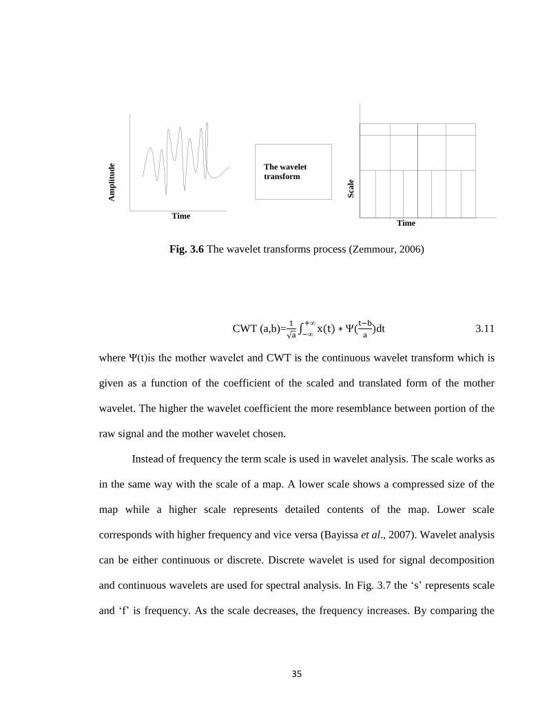
Fig. 3.6 The wavelet transforms process (Zemmour, 2006)

CWT (a,b)=

√ ∫

dt 3.11

where (t)is the mother wavelet and CWT is the continuous wavelet transform which is

given as a function of the coefficient of the scaled and translated form of the mother

wavelet. The higher the wavelet coefficient the more resemblance between portion of the

raw signal and the mother wavelet chosen.

Instead of frequency the term scale is used in wavelet analysis. The scale works as

in the same way with the scale of a map. A lower scale shows a compressed size of the

map while a higher scale represents detailed contents of the map. Lower scale

corresponds with higher frequency and vice versa (Bayissa et al., 2007). Wavelet analysis

can be either continuous or discrete. Discrete wavelet is used for signal decomposition

and continuous wavelets are used for spectral analysis. In Fig. 3.7 the „s‟ represents scale

and „f‟ is frequency. As the scale decreases, the frequency increases. By comparing the

The wavelet

transform

Time

Sca

le

Time

Am

pli

tud

e

36

signals when s=1 and s=0.05 it can be seen that the frequency is highest (f=20) when the

scale is lowest(s=0.05).

Fig. 3.7 Relationship between scale and frequency in wavelet transform

Fig. 3.8 Translation of a mother wavelet along a signal for a s=1(Polikar, 2001)

37

In wavelet analysis translation is moving the mother wavelet across the signal for

each scale that is considered. From Fig.3.8 at a scale of (s=1), the window or the mother

wavelet continuously moves along the time axis. Four different location of the wavelet is

shown when it is at 2sec, 40sec, 90sec, and 140 sec, respectively. The whole signal is

multiplied by each scale at different locations as in Eq. (3.9) of the mother wavelet and a

higher value indicates that the signal contains more of the attributes of the multiplying

wavelet.

Fig. 3.9 Translation of a mother wavelet along a signal for a s=5 (Polikar, 2001)

As illustrated in Fig. 3.9 the scale of the wavelet has increased from s=1 to s=5

(lower frequency mother wavelet) compared to Fig 3.8. The signal is multiplied by this

scale at different positions, and it will pick up the lower frequency components of the raw

signal.

38

The goal in Wavelet transform is to turn the information of a signal into numbers

which are coefficients that can be manipulated, stored, transmitted, analyzed or used to

reconstruct the original signal (Zhu et al., 2007). Wavelet transform is aimed at

converting information contained in a time-series signal in to wavelet coefficients so that

one can detect changes in the analyzed and transformed coefficients which might be

hidden in the raw time series signal. These coefficients can be represented in a graphical

representation called scalogram. A scalogram is time (translation)-scale (frequency)

representation of a transformed signal where a coefficient is computed for each

combination of scale and translation. The color intensity represents the wavelet

coefficients. A bright color corresponds to a higher wavelet coefficient; this in turn

represents a strong correlation between the signal and the wavelet applied (Pokilar,

2001). Therefore a strong correlation or higher wavelet coefficient or brighter color

intensity means that a portion of the signal resembles the wavelet.

3.2.3 Hilbert-Huang Transform(HHT) and Emperical Mode Decompositon(EMD)

3.2.3.1 Hilbert Huang Transfrom(HHT)

HHTtakes a function u(t) as an input and produces a function, H(u)(t), with the

same domain. Hilbert transform has got a wide application for data which are non-

stationary and non-linear (Huang and Attoh-Okine , 2005).

∫

∫

) 3.12

where H(u)(t) is the Hilbert transform of u(t), and u(t) is any real valued function, p.v. is

the principal value of the singular integration.

39

Hilbert transform can also be described by the equation,

z(t)= x(t)+j y(t) = a(t) 3.13

where a(t) is the instantaneous amplitude and is given by

a(t) =√ 3.14

is the phase function and the phase angle from which the instantaneous frequency is

calculated as given by Eq. (3.7) and Eq.(3.8).

=

3.15

f= (1/2 (

) 3.16

One advantage obtained with the representation in Eq. (3.16) is that frequency can

be determined at any given time t, since frequency can be calculated by differentiating

the phase angle with respect to time (Huang and Attoh-Okine, 2005).

The following example illustrates the effect of having a zero mean in the

application of Hilbert transform. All the three functions are the same sinusoidal function

except for mean shifted by 0.5 and 1.5 as shown in Fig.3.10.

Example on Hilbert transform: Consider three signals given by a =sin x +α, for α

= 0, 0.5, 1.5 from which we can have three different sinusoidal signals: sin x, sin x+0.5

and sin x+1.5 (Huang and Attoh-Okine, 2005).

The first step in the extraction of instantaneous frequency is transformation of the

signal by using Hilbert transform to obtain the phase plane diagram inFig.3.11. From the

plane or phase diagram, phase angle is withdrawn as depicted in Fig.3.12 by

differentiating the phase angle with respect to time and instantaneous frequency is

obtained using Eq. (3.16).

40

Fig. 3.10 Time series plots of signals of sin x +α, for α =0, 0.5, 1.5

From the three sinusoidal plots of the three signals with identical shape but

different mean values, it is obtained that the frequency is positive and constant for the

signal (sin x) with zero mean as shown in Fig.3.13. For the (sin x+ 0.5) signal the

frequency is not constant and for the third signal which is (sin x +1.5) the frequency

fluctuates between negative and positive values.

This example shows that the instantaneous frequency gives a meaningful value

when a signal such as a sine function is symmetrical with respect to the zero mean.

Therefore, to obtain Hilbert transform and hence instantaneous frequency, the raw signal

should have a mean value symmetrical with respect to zero. To accomplish this purpose,

a signal should be analyzed using Empirical Mode Decomposition (EMD) prior to

applying the Hilbert Huang transform.

41

Fig. 3.11 Hilbert transform of sin x+ α for α =0, 0.5, 1.5

Fig. 3.12 Phase angle of sin x+ α for α =0, 0.5, 1.5

42

Fig. 3.13 Instantaneous frequency of sin x+ α for α =0, 0.5, 1.5

3.2.3.2 Empirical Mode Decomposition (EMD)

EMD is a fundamental and is a necessary step to reduce any given data in to a

collection of intrinsic mode functions (IMF) to which the Hilbert analysis can be applied

(Huang and Attoh-Okine, 2005). An IMF represents simple oscillatory mode embedded

in the raw data where each IMF deals with only one mode of oscillation with no complex

riding waves present. Since most data does not represent IMF naturally the Hilbert

transform is not capable of producing full description of frequency if the data contains

more than one oscillatory mode at a particular time. Due to this reason, data should be

decomposed in to independent IMF components.

43

Sifting is the process of decomposition of a signal in to its IMF components by

using Empirical Mode Decomposition (EMD). The sifting process can be explained by

the following steps.

Step1. Assume a signal x(t) is given to be sifted by EMD. Find all the upper and

lower peak points of the signal and create upper and lower envelop by

interpolation. The upper envelop can be denoted by emax(t) and the lower

by emin(t) and take the average of the envelopes emax(t) and emin(t) to get

m1Fig. 3.15a.

Step 2. Subtract the envelope mean m1 from the original signal. This is shown on

Fig.3.15b as h1=x(t)-m1.

After this step check if the new data h1 has fulfilled the criteria for IMF or not

and if h1 is not IMF, repeat the steps given by 1 and 2.

The criteria for a sifted signal to be IMF is

i. When number of extrema(maxima+minima) and zero crossings are the same or

differ by one and

ii. Envelopes as defined by all the local maxima and minima are being symmetric

with respect to zero (Huang et el. 2005).

The sifting process should stop when the SD (standard deviation) between two

consecutive sifted signals is smaller than a preset value given by Eq.(3.14).The original

signal(data) to be sifted x(t) can be represented by Eq. (3.15) which illustrates the

decomposition of x(t) in to n-IMF components(Cj) and a residue(rn).

44

Fig. 3.14(a) The cubic spline upper and the lower envelopes and their mean h1

(Huang and Attoh-Okine, 2005)

Fig. 3.14(b)Comparison between data x(t) and h1

(Huang and Attoh-Okine, 2005)

45

Fig. 3.14(c) Repeat the sifting process using h1 as data

(Huang and Attoh-Okine, 2005)

In Eq.(3.14) ( ) represents two consecutive sifted signals.

The residual rn, can be either a constant, monotonic mean trend or a curve having only

one extrema point.

∑( )

3.17

x(t)= ∑ +rn 3.18

IMFs have are always symmetrical with respect to the local mean and have a

unique local frequency different from the rest of the other IMFs. Fig. 3.15 summarizes

the steps to be followed in the EMD sifting process in the form of a flow chart.

46

Fig. 3.15 Flow chart showing the steps in EMD (Zemmour, 2006)

47

3.2.4 Comparison of Fourier, Wavelet, and Hilbert Transform

For the purpose of comparison consider a chirp signal which changes frequency

continuously with time.

Fig. 3.16 Time series plot of a chrip signal

Fig. 3.17 Fourier transform of chrip signal

48

Fig. 3.18 Continuous wavelet transform of the chrip signal

Fig. 3.19 Instantaneous frequency plot of the chrip signal

The Fourier transform of the chrip signal Fig 3.17 shows the high frequency

components with a horizontal line with no information at what time the frequencies

occur. The spectrogram in Fig. 3.19 illustrates graphically that the low frequency

components of the signal occur at an early stage by indicating it with higher scale values.

The scale of bright line goes decreasing through time in the spectrogram implying an

increase in frequency since a decrease in scale represents an increase frequency. Whereas

49

the instantaneous frequency Fig. 3.19 which is the product of Hilbert transform

demonstrates that the frequency increases constantly with time. One advantage of this

representation over the continuous wavelet transform is that, the frequency at the desired

instant of time can be obtained.

Therefore Hilbert transform looks the favorite candidate among the spectral

analysis tools. Table 3.3 revises the advantage and disadvantages of the three frequency

domain approaches.

Table 3.2 Comparison between the different frequency domain analysis methodologies

FOURIER WAVELET HILBERT HUANG

Basis A priori A priori Adaptive

Frequency

Convolution:

global, uncertainty

Convolution:

Regional, uncertainty

Differentiation:

local, certainty

Presentation Energy-frequency Energy-time-frequency Energy-time-frequency

Non linear No No Yes

Non Stationary No Yes Yes

Feature extraction No Discrete: No Continuous: yes Yes

50

CHAPTER IV

IMPLEMENTATION OF PROPOSED METHOLOGIES

4.1 Data Sources for Analysis

In order to validate the proposed methodologies of data analysis tools, simulation

data and data from a functional (working) bridge were applied. This chapter explains the

application of the proposed methodologies, to data sources obtained from two different

sources. Spectral analysis of a benchmark problem simulation data is presented in the

first section followed by statistical analysis and time series modeling for the bridge data.

4.1.1 Data Source from Bridge

For the purpose of time series analysis data was obtained from strain gauge

sensors installed on a bridge found in Texas. Four sensors were mounted on two of the

supporting columns of the bridge since 2001. Apart from deformation measurements,

temperature at each of the sensors was also measured by the strain gauge sensors. The

data obtained contains three years full data from 2002-2004 and partial year data for year

2001 and 2005 measured every hour of a day.

51

Strain gauge

mounted on the column

Fig. 4.1 Supporting column of the bridge

4.1.2 Data Source from Simulation

Data obtained from a 4-storey and 2-bay by 2-bay steel frame scale model

structure as shown in Fig. 4.2 designed by theAmerican Society of Civil

Engineers(ASCE) for the purpose of SHM was gathered to show validity of the spectral

analysis approaches. The structure is located in the earthquake engineering research

laboratory at the University of British Colombia (UBC) (Johnson et al., 2004). In this

52

study to excite the structure the cases considered were electrodynamic shaker,impact

hammer, and ambient excitation.

Fig. 4.2 Picture and 3D model showing the bench mark problem building

(Johnson et al., 2004)

For the electrodynamics shaker excitation, the shaker was placed on top floor the

structure with a capacity of 311 N (Dyke et al. 2003). To capture the response of the

structure accelerometers were placed throughout the structure in the structure‟s weak(y-

direction) and strong (x-direction). Based on the experiments conducted in the earthquake

laboratory, a Matlab algorithm by the name „DATAGEN‟ was developed to simulate the

real conditions of the experiment (Lin et al., 2005).

53

4.2 Frequency Domain Analysis of Simulation Data

The bench mark structure from which simulation data was taken is a 2.5 m by

2.5m floor area and 3.6 m high Fig. 4.2. A bracing system placed along the diagonal was

fixed for each bay and to emulate a real structure a concrete slab was built at each floor

and the removal of these braces is designed to simulate damage to the structure. For the

experiment wind ambient excitation and another two types of forced excitation sources

were introduced (Dyke et al., 2003). Impact hammer test and electrodynamics shaker

were applied for the forced excitation case. A more detailed description of the bench

mark structure problem can be found in (Johnson et al., 2004). One undamaged case and

six damage patterns were the subject of study of this benchmark problem. Matlab code by

the name „DATAGEN‟ is used to run the simulation according to the damage patterns

shown in Table 4.1 and Fig. 4.3.

Table 4.1 Damage patterns and their description considered in the Matlab program

(Johnson et al., 2004)

Damage case Description(method of execution)

Pattern-1 Removing all the braces in the 1st floor

Pattern-2 Removing all the braces in the 1st and 3

rd floor

Pattern-3 Removing one brace in the 1st floor

Pattern-4 Removing one braces from both the 1st and 3

rd floor

Pattern-5

Removing one braces from both the 1st and 3

rd floor

plus one of the beams partially unscrewed from the

column

Pattern-6 Area of one brace in the 1stfloor reduced to 2/3

54

Fig. 4.3 Six damage patterns defined by the Benchmark problem (Johnson et al., 2004)

The six damage patterns used for the simulation are revised in Table 4.1. Fig. 4.4

explains the each damage patterns graphically. Table4.2 summaries four different cases

considered for demonstration of the spectral analysis approaches obtained by applying

the Matlab program (DATAGEN) provided by the study group, (Lam, 2000).

Four different cases were devised to test the validity of the frequency domain

approaches. The first one is data withdrawn from the undamaged state of the structure by

applying the default parameters of the Matlab program. The second case is obtained by

running the simulation for damage pattern-2 which is removing all the braces from the 1st

and 3rd

floor. The third case considered is data from damaged condition but with a less

damage extent (pattern-1) simulated by removing the braces on the 1st floor as shown in

55

Table 4.2 Different damage scenarios considered

Table 4.2. Case-4 is the combination of damaged (pattern-2) and undamaged conditions

of the bench mark structure. There were 4 accelerometer sensors installed on each floor

of the structure (Lam, 2000).

The sampling frequency taken for all the different cases is 1000Hz and the time

span of the simulation is 40 sec. In this study simulation data from the 4th

floor were

considered. The time series plot, the Fourier transform and, 2D&3D wavelet plots are

presented in the following sections.

Case Damage status Damage pattern

1 Undamaged Undamaged(No braces removed)

2 Damaged Removing braces 1st and 3

rd floor

3 Damaged Removing braces from 1st floor

4 Mixed cases Combination of case-1 and case-2

56

Fig. 4.4 Time series plot of the damage scenarios considered (case1-case 4)

57

Fig. 4.5 Fourier transform of the four cases (case1-case 4)

58

Fig. 4.6 Wavelet transform (2D) of the four cases (case1-case 4)

59

Fig. 4.7(a) 3D-wavelet transform for case-1

Fig. 4.7(b) 3D-wavelet transform for case-2

60

Fig. 4.7(c) 3D-wavelet transform for case-3

Fig. 4.7(d) 3D-wavelet transform for case-4

61

4.2.1 Fourier Transform of Simulation Data

From the Fourier transform in Fig. 4.5 each of the different cases seem to have 4-

frequency mode components except for case-4. Table 4.3 shows the magnitudes of the

four frequency modes obtained from each case. From the numbers one can understand or

observe that the frequency obtained from the damaged data sources is less than data

simulated from the undamaged. The amount of reduction varies for the different damage

cases. For example each of the four frequency values for case-2 are less than case-3

implying that data induced from damage scenario case -2 is more severe that of case-3.

Case-4 has more frequency mode components but the dominant values are as shown in

Table 4.3.

Table 4.3 Fourier transform output values for the four damage cases

Case 1 Case 2 Case 3 Case 4

Frequency mode 1 8.565 4.66 5.02 4.64

Frequency mode 2 20.24 11.97 17.18 11.83

Frequency mode 3 30.77 28.93 29.86 31.34

Frequency mode 4 38.32 32.06 38.32 33.26

Fig. 4.8 presents a summary of the frequency comparison of the four damage

scenarios considered for the case study. From the figure it is apparent and imperative to

expect that the frequency extracted from the undamaged case is higher compared with

those from the damaged status. It also shows that the frequency gets even lower and

lower as more severe damage is introduced to the structure.

62

Fig. 4.8 Comparison of frequency from Fourier transform for the four damage cases

4.2.2 Wavelet Analysis of Simulation Data

From the scalogram plots of the four different damage cases shown in Fig. 4.6 and

Fig. 4.7 one can compare and contrast the scale-translation representation both in 2D and

3D. The 2D plot shows only two axes: scale and time. The coefficients for each scale and

combination are represented as color intensity. The 3D plots shown in Fig 4.7(a) - Fig

4.7(d) shows the wavelet transform in scale, time and coefficient axes unlike the 2D plots

where the coefficients are represented in terms of color intensity.

In wavelet analysis a higher scale means lower frequency and vice versa. From

wavelet transform of damage case-2 as shown in Fig.4.7(b) the peaks starting from

around a scale of 81 to higher scale shows that the frequency has decreased and also the

coefficient of lower scale values(higher frequency components)has decreased. While in

63

damage case-4 the scale starts to increase after around 20 sec which indicate that damage

was introduced after 20 sec which is consistent with the simulation data. For the first 20

sec the plots for case-1 and case-4 looks almost the same as in Fig 4.7(a) and Fig 4.7(d).

By computing the coefficients at each scale of the simulation data, we can

compare the plots both in 2D and 3D and observe the changes in the scale which

indirectly represents frequency. One advantage that is gained by using wavelet analysis

for this case study time information is available unlike the Fourier transform. In damage

case 4 which is a combination of undamaged and damaged simulation data, it can be seen

that around the 20 sec, the scale starts to increase indicating a frequency decrement and

hence damage introduction to the structure.

4.2.3 Hilbert-Huang Application to Simulation Data

The four cases introduced in Table 4.2 were also considered to show the validity

of the Hilbert Huang transform. Empirical Mode Decomposition (EMD) is applied to the

different cases prior to Hilbert-transform and instantaneous frequency computation for

each of the four cases. Fig 4.11 shows the Intrinsic Mode functions (IMFs) for case-1.

From the computation of EMD it is found out that the signal from the undamaged

case has 11 IMFs. The Hilbert transform is computed for the first and second IMFs to

obtain the phase diagram. From the phase diagram phase angle is computed. By

differentiating the phase angle we can finally compute the instantaneous frequency which

is the feature extraction or damage indicator which we are looking for. Recall the

relationship between phase diagram, phase angle and instantaneous frequency from

64

Fig. 4.9 IMF components of case-1 after EMD of the acceleration signal

section 3.2.3 of chapter 3.The same procedure is followed for the rest of the damage

cases and the instantaneous frequency is extracted and the final output is as shown in Fig

4.10. The steps followed for the Hilbert transform can be revised in the following steps,

i. Sifting of a signal in to IMFs by using EMD

ii. Hilbert transform and Instantaneous frequency computation for IMFs.

From the instantaneous frequency plots (cases 1-4) from Fig. 4.10 it is difficult to

see the difference in magnitude of frequency plotted for the damaged and undamaged

cases. To be able to decide there is a difference in mean and variance from the cases

considered, a statistical hypothesis test was conducted.

65

(iv) Instantaneous frequency plot for case-1(IMF-1) (b) Instantaneous frequency plot for case-2(IMF-1)

(c)Instantaneous frequency plot for case-3(IMF-1) (d) Instantaneous frequency plot for case-4(IMF-1)

Fig. 4.10 Instantaneous frequency plot for (case-1-case-4) from the 1st IMF of each case

66

Statistical Hypothesis testing

In statistics hypothesis testing is done to draw inferences about a population based

on statistical evidence from a sample. The instantaneous frequency values from the

samples that were taken in the damaged (cases 2, 3, and 4) and undamaged condition

(case-1) from the plots could not tell us if there is shift in mean and variance when

damaged is introduced. Since the data being investigated are generated from two separate

and independent groups (damaged and undamaged), the two tailed T-test for mean

change and variance change was selected for the test.

Hypothesis testing for Mean change in the instantaneous frequency:

Null Hypothesis

H0: mu1-mu2=0 or (mu1=mu2) with unknown variance

No mean change in the instantaneous frequency

Alternate Hypothesis

H1: mu1-mu2 ≠ 0 or(mu1≠mu2)

There is change in the mean of the instantaneous frequency

where mu1 and mu2 represents the mean values from different and independent cases.

From Matlab statistical tool box the function h = ttest2(x, y) was selected to

perform a t-test of the null hypothesis. The t-test assumes that x and y (the cases to be

compared) are independent random samples from normal distributions. The result of the

test is returned in h. h=1 indicates a rejection of the null hypothesis at the 10%

significance level. h = 0 indicates a failure to reject the null hypothesis at the 10%

significance level.

67

Hypothesis testing for variance change in the instantaneous frequency:

Null Hypothesis

H0: s21-s

22 =0 or (s

21= s

22)

No change in the variances of the frequency from two different cases

Alternate Hypothesis

H1: s21-s

22≠0 or (s

21≠ s

22)

There is change in the variances of the instantaneous frequency

where σ2

1and σ2

2 represents the sample variances from two independent set of data

(frequency) to be compared.

From Matlab statistical tool box the function h = vartest2 (x,y) was selected to

performs a t-test of the null hypothesis that the variances from two independent samples

are the same. The result of this test is returned in h. h = 1 signifies a rejection of the null

hypothesis at the 10% significance level where as h = 0 indicates a failure to reject the

null hypothesis at the 10% significance level.

A Matlab algorithm was developed to do the hypothesis testing with a

significance level of (α=0.1) that tests the null hypothesis every 1 sec for the whole time

span of the sample data series which is 40 sec. Note that since the main focus here is to

compare sample frequency changes in(mean and variance) from two different scenarios

one damaged and the other undamaged and as a result, each of the three damaged

conditions (case 2, 3, and 4) will be compared with the undamaged state (case-1).

68

Fig. 4.11 Two sample (case1&case2) Variance test

Fig. 4.12 Two sample (case1&case2) Mean test

Fig. 4.13 Two sample (case1&case3) Variance test

69

Fig. 4.14 Two sample (case1&case3) Mean test

Fig. 4.15 Two sample (case1&case4) Variance test

Fig. 4.16 Two sample (case1&case4) Mean test

70

From the hypothesis test results of change in mean and variance between case1

(undamaged) and the rest of the three cases (damaged), it is found out that the null

hypothesis is rejected successfully as summarized in Table 4.4. The rejection of the null

hypothesis implies that there is a difference in mean and variance from the two cases

under study. For example the 90% rejection rate in variance test (case1 &case2)

illustrates the frequency obtained from the two cases are different which is normal to

expect since one is coming from a damaged and the other form undamaged case.

Table 4.4 Success rate of the mean and variance test in rejecting the null hypothesis

The higher successful rejection rate of case 2 compared with case3 shows that the

proposed methodology is more sensitive and effective in differentiating between two

cases as severe damage is introduced. Moreover it can be observed that the Variance test

which measures the hypothesis, if two different distributions obtained from damaged and

undamaged have the same variance or not, is shown to be more effective in successfully

rejecting compared with the mean test.

Table 4.5 summarizes the output of variance and mean test conducted for other

IMFs. From the table it can be observed that the successful rejection rate both by the

Case1&Case2 Case1&case 3 Case1&case4

Variance test 90% 80% 95%

Mean test 87% 65% 95%

71

mean and variance of the hypothesis testing tends to increase when the comparison of

instantaneous frequency is made for the 2nd

, 3rd and 4th

IMF values.

Table 4.5 Success rate of the mean and variance test in rejecting the null hypothesis from

IMF-1 to IMF-4

Case1 & Case2 Case1 & Case3 Case1 & Case4

Mean test Variance test Mean test Variance test Mean test Variance test

1st IMF 87% 90% 65% 80% 95% 95%

2nd

IMF 85% 92.5% 85% 87.5% 90% 65%

3rd

IMF 95% 95% 92.5% 98.5% 90% 85%

4th

IMF 97.5% 100% 97.5% 92.5% 95% 95%

A new case study (case-5) is created to show the efficiency of the proposed

methodology of combining Hilbert transform and hypothesis testing to detect the

progress from less severe to more severe damage. This case study is a combination of

simulated data which comes from undamaged state, damage pattern-5, damage pattern-2

and damage pattern-1 which is described in Table 4.1. Note that the severity of damage

increases one move from the 1-10 sec interval to the 31-40 sec interval.

Table 4.6 Damage patterns for case-5

Time period(sec) Damage pattern

1-10 Undamaged(No braces removed)

11-20

(pattern-5).Removing one brace from the

1st and 3

rd floor plus one of the beams

partially unscrewed from the column

21-30 (pattern-1).Removing all braces in the 1

st

floor

31-40 (pattern-2).Removing all braces in the 1

st

and 3rd

floor

72

The instantaneous frequency obtained from case-5 is compared with case-1 (obtained

from data from undamaged situation) to observe the change in mean and variance

between the two cases.

The result of the hypothesis test shows the change in the mean from the

comparison of case-5 and case-1 is observable with time. The significance level for the

hypothesis test is taken as (α=0.1). If the p-value of the test is less than 0.1 the null

hypothesis is rejected and this rejection is line is represented by the dotted line as in Fig

.4.17. From Fig.4.17 the majority null hypothesis (60%) is not rejected which shows that

the data from for the first 10 sec is from undamaged since it is compared with case 1. For

the time interval between 11-20 sec there is 80% rejection rate of the null hypothesis

which indicates the mean of frequency has changed as a result of damage introduction.

The 21-30 sec interval indicates a 90% rejection rate as data is coming from a more

severe damage situation. Finally the 100% rejection rate of the null hypothesis indicates

that the mean of the frequency from the cases of damaged and undamaged scenarios for

the interval 31-40 sec are different. It is observed that the level of rejection of the null

hypothesis varies for instantaneous frequencies obtained from different

From the application of Hilbert transform and hypothesis testing to the simulation

data, change in the mean and variance (dispersion) of instantaneous frequency can be

detected in with the inclusion of time information

By observing the mean and variance test plots from two different and independent

instantaneous frequency plots, we can indicate at what time the difference in frequency

occurs. Compared with the Fourier transform and wavelet analysis, the Hilbert transform

together with the statistical hypothesis testing gives more information by quantifying the

73

damage level by indicating the successful rejection rate of the observed change in mean

and variance of the instantaneous frequency.

Fig. 4.17 Two sample mean test (case-1&case-5)

4.3 Statistical Analysis of Bridge Data

In this section measurements from different sensors are investigated using

statistical tools to understand underling trends on the measured strain and temperature.

Besides, the relationship between temperature and strain recordings is examined. The

terminologies clomn-1 and column-2 are used throughout this section to differentiate

between the two columns of the bridge.

To investigate the similarities and differences among the 4-sensors of column-1 a

time series is plotted as shown in (Fig.4.19). From the plot it can be clearly seen that the

74

magnitude of deformation values for the 4-senosr varies with sensor 4 being with the

highest magnitude of deformation followed by sensor-1, sensor-3 and sensor-2

respectively in descending order. The deformation recordings from sensor 4 are

approximately 6 times larger than that of sensor-2.The same kind of deformation

recordings variation is observed for column-2.

Fig. 4.18 Comparison of strain measurement from the 4 sensors of column-1

The correlation matrix given in Table 4.7 shows there is a significant relationship

between the measured strain values of the four sensors. The correlation coefficient shown

in the matrix is a single number which lies between -1 and +1 and it shows how strong

the relationship between two variables is. A correlation coefficient (r) close to +1 shows a

strong relationship between the two variables. Assuming we have two variables X and Y,

the strength of the correlation coefficient r, is as interpreted in Table 4.8. The matrix plot

75

in Fig. 4.19 also proves the fact that the sensor strain recordings are correlated which is

shown in terms of lines. The more the straight the line, the higher the correlation.

Table 4.7 Correlation coefficient among the 4-sensors

Column-1(correlation)

sensor-1 sensor-2 sensor-3 sensor-4

sensor-1 1.00000

sensor-2 0.86184 1.00000

sensor-3 0.90971 0.90205 1.00000

sensor-4 0.99155 0.84125 0.89387 1.00000

Table 4.8 Summary of correlation coefficient values

Correlation

coefficient Interpretation

r = + 1.0 As X goes up, Y always also goes up

r = + 0.5 As X goes up, Y tends to usually also go up

r = 0 No correlation

r = - 0.5 As X goes up, Y tends to usually go down

r = - 1.0 As X goes up, Y always goes down

76

Fig. 4.19 Matrix plot showing the correlation among the 4-sensors

Fig. 4.20 Time series plot for the temperature readings at the 4-sensors from Column-1

77

From the plot of the temperature at each sensor of column-1, there is not only

seasonality but also a very high amount of correlation between the sensor measurements.

Seasonality is the periodic variation of a measured value over time. The temperature

recordings are higher during the summer time and lower in the winter season. The

correlation between the temperature measurements range between coefficient of

correlation (r) value of 0.993 and 0.997.This implies that when the temperature measured

at one sensor decreases (increase) so do the rest of the other sensor measurement values.

Relationship between sensor deformation measurement and temperature:

To study the relationship between temperature and strain readings, one sensor was

selected. In Fig. 4.21, the standardized time series plot of deformation data for three

years (2002-2004) and temperature measurement at the sensor location is illustrated.

From the plot it can be clearly seen that there is seasonality with the temperature

recordings where as for the strain data seasonality is observed after the data is de-trended.

In time series analysis detrending is removing the slowly increasing or decreasing values

or trend from a sequence of measured variables. The correlation coefficient between

temperature and strain, r, is found to be around 0.275 before detrending of the strain data.

After detrending of the sensor data the correlation between temperature and strain is

found to be improved to r = 0.5218.

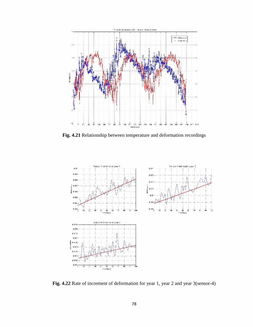
78

Fig. 4.21 Relationship between temperature and deformation recordings

Fig. 4.22 Rate of increment of deformation for year 1, year 2 and year 3(sensor-4)

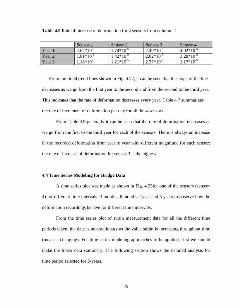
79

Table 4.9 Rate of increase of deformation for 4 sensors from column -1

From the fitted trend lines shown in Fig. 4.22, it can be seen that the slope of the line

decreases as we go from the first year to the second and from the second to the third year.

This indicates that the rate of deformation decreases every year. Table 4.7 summarizes

the rate of increment of deformation per day for all the 4-sensors.

From Table 4.9 generally it can be seen that the rate of deformation decreases as

we go from the first to the third year for each of the sensors. There is always an increase

in the recorded deformation from year to year with different magnitude for each sensor;

the rate of increase of deformation for sensor-3 is the highest.

4.4 Time Series Modeling for Bridge Data

A time series plot was made as shown in Fig. 4.23for one of the sensors (sensor-

4) for different time intervals: 3 months, 6 months, 1year and 3 years to observe how the

deformation recordings behave for different time intervals.

From the time series plot of strain measurement data for all the different time

periods taken, the data is non-stationary as the value strain is increasing throughout time

(mean is changing). For time series modeling approaches to be applied, first we should

make the linear data stationary. The following section shows the detailed analysis for

time period selected for 3-years.

Sensor-1 Sensor-2 Sensor-3 Sensor-4

Year 1 2.62*10-5

1.74*10-5

2.40*10-5

4.02*10-5

Year 2 1.81*10-5

1.42*10-5

2.82*10-5

3.28*10-5

Year 3 1.18*10-5

1.21*10-5

2.37*10-5

1.17*10-5

80

Fig. 4.23 Time series plot for sensor-4 with different time period

The time series analysis contains four main steps which are time series plotting,

model identification, parameter estimation and diagnostic checking.

Step1: Time Series Plotting

From Fig. 4.24 since the data is non-stationary we should be able to find a way to

make it stationary. Power transformations are applied to improve the interpretability of

data or appearance of graphs. A Box- Cox test was employed to identify what kind of

power transformation is appropriate to the data. Based on the test from Fig.4.25 the type

of transformation that we should use is taking the square of the raw time series data. The

95% confidence interval for λ contains a value closer to 2, and this strongly suggests

taking the squared value for the sensor data.

81

Fig. 4.24 Time series plot for sensor-4 (3-years)

Step2: Model Order Selection

Since the data is non-stationary we should take the first differencing as in Fig

4.25.To support the decision for taking the differencing, the augmented Dickey-Fuller

(ADF) test statistic was performed. The null hypothesis test for ADF is that the data to be

tested is non-stationary while the alternate hypothesis being data is stationary. By running

this test for the squared sensor data at a significance level of α=0.1 it is found that the p

value is 0.7905 which fails to reject the null hypothesis. This suggests the hypothesis that

the data stationary holds valid.

82

Fig. 4.25 Box-Cox plot for sensor-4

Assume that x(t) is data for sensor-4 taken for 3 years , from the Box-Cox test we

knew that we have to take the square of the data, and let y(t)=x(t)2. The expression

diff(y(t)) indicates that a differencing is taken for the time series data y(t) and it can be

defined by diff(y(t))= y(t)=y(t)-y(t-1). The plot for the diff(y(t)) is illustrated in Fig. 4.26.

The main task in this step is determining the order of the model by plotting the

partial autocorrelation (PACF) and autocorrelation (ACF).

From Fig.4.27 the ACF plot seems tailing off slowly which makes it uncertain to

determine the order for MA process (q). The PACF plot shows the values seem to cut off

after lag p=2 but there is significant correlations between lags and 10. To determine the

correct order for the model, the extended autocorrelation function (EACF) was performed

to get the values shown on Table 4.10. From the EACF select a triangular region of 0

values (shown in Table 4.10) and start from the top left vertex which gives the least

combination of AR and MA model parameters. From the possible combination of AR and

MA orders, select orders with the least p and q value. From the possible combination the

model orders (p,d,q) , (3,1,2) and (1,1,4) seems a valid model.

83

Fig. 4.26 Time series plot for diff(y(t))

Fig. 4.27 ACF and PACF plot for diff(y(t))

84

Step 3: Parameter Estimation

Once we have identified the model orders the next step is estimation of the

parameters. The R-statistical software output of the two model orders selected, i.e.

c=(3, 1, 2) and c= (1, 1, 4) are as shown in Fig. 4.28.

Table 4.10 Sample extended autocorrelation function (EACF) for diff(y)

AR/MA 0 1 2 3 4 5 6 7 8 9 10 11 12 13

0 X X X X X 0 0 X 0 0 X X 0 0

1 X X X X 0 0 0 X 0 0 0 X X 0

2 X X X X 0 0 0 X 0 0 0 0 0 0

3 X X 0 0 X 0 0 X 0 0 0 0 0 0

4 X X 0 0 X 0 0 X 0 0 0 0 0 0

5 X X X 0 0 0 0 0 0 0 0 0 0 0

6 X X X X 0 X 0 X 0 0 0 0 0 0

7 X X X X X X X X X X X 0 0 0

8 X X X X X X 0 0 X X X 0 0 0

85

(a)c=(3,1,2) (b) c=(1,1,4)

c)c=(2,1,2)

Fig. 4.28 R-output for parameter estimation for model orders c=(3,1,2) c=(1,1,4) and

c=(2,1,2)

Call:

arima(x = y, order = c(3, 1, 2))

Coefficients:

ar1 ar2 ar3 ma1 ma2

1.0031 -0.4295 0.0356 -0.5838 -0.2542

s.e. 0.1368 0.1614 0.0838 0.1342 0.1110

sigma^2 estimated as 1.085e-09:

log likelihood = 9737.98,

aic = -19465.96

Call:

arima(x = y, order = c(1, 1, 4))

Coefficients:

ar1 ma1 ma2 ma3 ma4

0.3151 0.1058-0.3966 -0.3205 -0.1065

s.e.0.0960 0.0960 0.0407 0.0464 0.0517

sigma^2 estimated as 1.089e-09:

log likelihood = 9736.37,

aic = -19462.75

Call:

arima(x = y, order = c(2, 1, 2))

Coefficients:

ar1 ar2 ma1 ma2

0.9485 -0.3636 -0.5309 -0.2969

s.e. 0.0464 0.0445 0.0470 0.0444

sigma^2 estimated as 1.086e-09:

log likelihood = 9737.9,

aic = -19467.81

86

From the order model c=(3,1,2) it can be seen that the coefficient for Ar-3 is not

significant implying there Ar-3 is non-existent in the model and due to this reason, it is

desired to fit a model of order C(2,1,2) whose parameters are estimated in Table 4.28(c).

The coefficients for the order=c(1,1,4) are all significant and finally we need to compare

model c=(2,1,2) and C(1,1,4) by comparing the AIC and log likelihood values. Based on

the AIC and log likelihood values the best model for diff(y) would be ARIMA (2,1, 2).

The model fitted can be written as in Eq.(4.1).

y2

(t)=0.9485y2

(t-1)+ 0.3636y2

(t-2)- 0.5309w2

(t-1)- 0.2969w2

(t-2)+ w(t)4.1

The fitted model ARIMA (2,1,2) is when three years of data is taken. The same

procedure is followed to fit a time series model considering only a one year data and the

model fitted is found to be ARIMA (0,1,2). This shows that the number of data points

taken has a huge effect on the final model selection.

Step 4: Model Diagnostics

This step is used to examine the goodness of fit of the selected model. If the

goodness of fit is poor, it is desired to redo the model fitting part again or time series

model may not be fitted at all. The residual which is the difference between the actual

and predicted model will be diagnosed to indirectly assess the validity of the selected

model. A model selection is deemed good if the model residual properties are close to

white noise.

From Fig. 4.29 the first plot that shows the standardized plot of the residuals

suggest a rectangular scatter around zero with no trend. This suggests that the residuals

are close to a white noise. The second plot indicates the autocorrelation of the residuals.

87

For a pure white noise these residuals should be uncorrelated and normally distributed

with zero means and some variance. Based on the autocorrelation plot of the residuals it

seems that it is uncorrelated which is a good indication that the selected model is

appropriate. The third plot illustrates that the hypothesis test that the residuals are

correlated is not rejected since the p-values are greater than the significance level. The

normality plot Fig. 4.30 also shows that the residuals follow a normal distribution except

for a slight distortion at the end points.

From the time series modeling for the bridge data it is noted that

(i) The model order selection is greatly affected by the number of data points. Two

different types of models were found for the same set of data but different number

of points. Taking 3 year data and 1 year data has resulted in model orders of c=

(2,1,2) and (0,1,2) respectively.

Fig. 4.29 Diagnostic plot for the fitted ARIMA c=(2,1,2) model

88

Fig. 4.30 Normality test for residuals

(ii) Based on the fitted model future recordings from the sensors can be compared

with the coefficients of the ARIMA model. The change in the coefficients of the

model will indicate the deviation from the base line of comparison. By monitoring

this change in coefficients, data can be analyzed if it is from a normal or damaged

state by comparing it from the undamaged state.

89

CHAPTER V

SUMMARY AND CONCLUSION

5.1 Summary of Findings

The proposed research was aimed at damage detection of civil structures bridges

based on response data from sensors. The applied damage detection methodologies were

time series modeling and frequency domain analysis. The validity of the approaches was

shown through application of simulation data designed on a benchmark problem by the

ASCE task group and data from a functional bridge. The case study of simulation data

considered in this research is aimed to show the capability of the proposed approaches to

determine the change in the frequency from different sources of simulated data.

According to the case studies conducted the frequency domain approaches were

shown to be effective on identifying the presence of abnormality (change in frequency)

from data captured from a damaged condition. In the study simulation data generated

from three different damage cases and one normal condition were considered. Simulated

data collected from the undamaged was taken as a baseline of comparison with the other

set of data from a damaged state. According to Huang et el., 2005, when damage is

introduced in to a system the dynamic behavior will change and this can be observed in

90

the modal parameters of the system such as frequency. Therefore, the main target in

transforming the raw acceleration time series data in to Fourier, wavelet and Hilbert

transform is to monitor the change in frequency from the data simulated from normal and

abnormal conditions.

Fourier transform of data from a normal and damaged condition of the civil

structure were compared and it is found out that the frequency obtained from a damaged

case were less in magnitude compared with the normal state. Since Fourier analysis lacks

time information we have no clue as to when the damage started to occur in the structure.

The wavelet analysis deals with the time information which is better than the

Fourier analysis. Damage case-4 defined in Table 4.2 is a combination of undamaged

data for the first 20 sec and damaged for the next 20 sec. The wavelet analysis applied to

this specific case for detecting the damage progress showed in the scalogram

representation that the scales of the transformed signal increases after 20 sec. This shows

that the method is able to capture the change in frequency after damaged is introduced in

the system.

EMD and Hilbert Transform for extraction of the instantaneous frequency

(frequency dependent on time) coupled with hypothesis testing were applied to the

simulation data. For the purpose of demonstration of the effectiveness of this approach

only analysis based on the first IMFs are shown in this study. In general the hypothesis

testing and Hilbert transform, detected the change in frequency of the cases in form of

rejecting and failure to rejecting the change in mean and variance of instantaneous

frequencies. From the two methods of hypothesis testing experimented, the change in

variance of the frequencies is found to be more effective and sensitive to successfully

91

reject the null hypothesis defined as no change in mean and variance of instantaneous

frequency. It is also observed that the Hilbert transform applied is dependent on the IMF

applied to get the instantaneous frequency.

In this research the formal procedures in time series procedures were applied to

data acquired from a functional bridge. It should be noted that the time series model

fitting is dependent on the number of data points taken for the analysis. It is observed that

taking different data sizes for the same sensor data will result in a different model order

selection. Based on fitted ARIMA models future deformation recordings from the sensors

can be forecasted which benefits in determining the extent of deformation and taking

proactive measures.

The statistical analysis has shown that there exists a high correlation between the

measured deformation values and different sensors. It is also shown that temperature and

deformation have a high correlation. Seasonality in the temperature recordings was

observed where as the deformation was observed to increase with time. From the analysis

it is observed that the level of deformation increment is dissimilar for different sensors.

5.2 Future Work

There are several barriers to the widespread use of sensors in bridges. One

significant problem is that there is scarcity of adequate data showing a failed bridge. Due

to this problem data analysis for bridges is limited to laboratory or experimentally

simulated data. The problem with using these kinds of data is that the actual operational

and environmental conditions at which the bridge experiences cannot be simulated well.

One reason to this problem is the capability of finite element simulation software since

92

environmental parameters such as temperature, wind; humidity etc. cannot be easily

incorporated into the model.

Due to this problem more advanced data analysis methodologies such as time

series analysis for non-stationary and non-linear data is the aim of future study. In this

study a series of approaches such as power transformation and differentiation were

applied to make the data stationary. It should be noted also that this process will conceal

the inherent feature of the data which will lead to a different results and conclusion. The

selection of optimal IMF for Hilbert transform and instantaneous frequency extraction is

the subject of future study due to the different outputs obtained by applying selected

IMFs.

93

REFERENCES

Problem Solving with Computers. from

http://www.isr.umd.edu/~austin/ence200.d/software.html

AASHTO. (2007). Bridge Design Specifications. Washington, DC.

Bassiuny, A., Li, X., & Du, R. (2007). Fault diagnosis of stamping process based on

empirical mode decomposition and learning vector quantization. International

Journal of Machine Tools and Manufacture, 47(15), 2298-2306.

Bayissa, W., Haritos, N., & Thelandersson, S. (2008). Vibration-based structural damage

identification using wavelet transform. Mechanical Systems and Signal

Processing, 22(5), 1194-1215.

Box, G. E. P., Jenkins, G. M., and Reinsel, G. C. . (1994). Time Series Analysis,

Forecasting and Control, (3rd ed.). Englewood Clifs, NJ. : Prentice Hall.

Carden, E., & Brownjohn,J. (2007). ARMA modelled time-series classification for

structural health monitoring of civil infrastructure. Mechanical Systems and

Signal Processing, 22, 295-314.

Chen, J., Xu, Y., & Zhang, R. (2004). Modal parameter identification of Tsing Ma

suspension bridge under Typhoon Victor: EMD-HT method. Journal of Wind

Engineering and Industrial Aerodynamics, 92(10), 805-827.

94

Doebling, W., & Farrar,C. . (1997). Using Statistical Analysis to Enhance Modal-Based

Damage Identification, in Structural Damage Assessment Using Advanced Signal

Processing Procedures. Paper presented at the Proceedings of DAMAS „97,

University of Sheffield, UK.

Fugate, M., Sohn, H., & Farrar, C. (2001). Vibration-based damage detection using

statistical process control. Mechanical Systems and Signal Processing, 15(4), 707-

721.

Hou, Z., Noori, M., & Amand, R. (2000). Wavelet-based approach for structural damage

detection. Journal of Engineering Mechanics, 126(7), 677-683.

Huang, N., & Attoh-Okine, N. (2005). The Hilbert-Huang transform in engineering:

CRC Press.

Huang, N., & Shen, S. (2005). Hilbert-Huang transform and its applications: World

Scientific Pub Co Inc.

Johnson, E., Lam,H.,Katafygiotis,L.,& Beck,J. (2004). Phase I IASC-ASCE Structural

Health Monitoring Benchmark Problem Using Simulated Data. Engineering

Mechanics, 130(1), 3–15.

Kullaa, J. (2003). Damage detection of the Z24 bridge using control charts. Mechanical

Systems and Signal Processing, 17(1), 163-170.

Lam, P. (2000). Matlab files for the Benchmark problem. from

http://bc029049.cityu.edu.hk/asce.shm/phase1/asce_linkspage.asp

Li, H., Zhang, Y., & Zheng, H. (2009). Hilbert-Huang transform and marginal spectrum

for detection and diagnosis of localized defects in roller bearings. Journal of

mechanical science and technology, 23(2), 291-301.

95

Li, Z., Chan, T., & Zheng, R. (2003). Statistical analysis of online strain response and its

application in fatigue assessment of a long-span steel bridge. Engineering

structures, 25, 1731-1741.

Li, Z., Wu, B., & Wang, Y. (2009). Statistical analyses on multi-scale features of

monitoring data from health monitoring system in long cable supported bridges.

Procedia Engineering, 1(1), 123-127.

Lin, S., Yang,J.,& Zhou,L. (2005). Damage identification of a benchmark building for

structural health monitoring. Smart Materials and Structures, 12, 162-169.

Mattson, S., & Pandit, S. (2006). Statistical moments of autoregressive model residuals

for damage localisation. Mechanical Systems and Signal Processing, 20(3), 627-

645.

Medda, A., Chicken,E. & DeBrunner,V. (2007). SIGMA-SAMPLING WAVELET

DENOISING FOR STRUCTURAL HEALTH MONITORING. 119-122.

Meo, M., Zumpano, G., Meng, X., Cosser, E., Roberts, G., & Dodson, A. (2006).

Measurements of dynamic properties of a medium span suspension bridge by

using the wavelet transforms. Mechanical Systems and Signal Processing, 20(5),

1112-1133.

National Transportation & Safety& Board. (2007). from

http://www.dot.state.mn.us/i35wbridge/index.html

Oh, C., Sohn, H., & Bae, I. (2009). Statistical novelty detection within the Yeongjong

suspension bridge under environmental and operational variations. Smart

Materials and Structures, 18, 1-9.

96

Omenzetter, O., & Brownjohn J. . (2006). Application of time series analysis for bridge

monitoring. Smart Materials and Structures, 15, 129-138.

Pai, P., Huang, l., Hu, J., & Langewisch, R. (2008). Time-frequency method for nonlinear

system identification and damage detection. Structural Health Monitoring, 7(2),

103-125.

Peng, Z., Tse, P., & Chu, F. (2005). A comparison study of improved Hilbert-Huang

transform and wavelet transform: Application to fault diagnosis for rolling

bearing. Mechanical Systems and Signal Processing, 19(5), 974-988.

Pines, D., & Salvino, L. (2006). Structural health monitoring using empirical mode

decomposition and the Hilbert phase. Journal of sound and vibration, 294(1-2),

97-124.

Polikar,R.(2001).TheWavelet Tutorial. from

http://users.rowan.edu/~polikar/wavelets/wtpart1.html

Report Card for America‟s Infrastructure. (2005). ASCE (American Society of Civil

Engineers), from http://www.asce.org/reportcard/2005/index.cfm.

Report Card for America‟s Infrastructure. (2009 ). ASCE (American Society of Civil

Engineers)from http://www.asce.org/reportcard/2009/

Rohrmann, R., Baessler, M., Said, S., Schmid, W., & Ruecker, W. (1999). Structural

causes of temperature affected modal data of civil structures obtained by long

time monitoring. Paper presented at the Proceedings of the XVII International

Modal Analysis Conference.

97

Shinde, A., & Hou, Z. (2004, June 30-July 2). A wavelet packet based sifting process and

its application for structural health monitoring. Paper presented at the American

Control Conference, Massachusetts.

Shumway, R., & Stoffer, D. (2000). Time series analysis and its applications: Springer

Verlag.

Sohn, H., Allen, D., Worden, K., & Farrar, C. (2005). Structural damage classification

using extreme value statistics. Journal of dynamic systems, measurement, and

control, 127, 125-132.

Sohn, H., Czarnecki, J., & Farrar, C. (2000). Structural health monitoring using statistical

process control. Journal of Structural Engineering, 126(11), 1356-1363.

Sohn, H., & Farrar, C. (2000a). Statistical process control and projection techniques for

damage detection.

Sohn, H., & Farrar, C. (2000b). Statistical Process Control And Projection Techniques

For Structural Health Monitoring.

Sohn, H., Farrar, C., Hunter, N., & Worden, K. (2001). Structural health monitoring

using statistical pattern recognition techniques. Journal of dynamic systems,

measurement, and control, 123, 706-711.

Sohn, H., Farrar,C.,Hemez,F.,Shunk,D.,Stinemates,D.& Nadler,R. (2003). A Review of

Structural Health Monitoring Litreature:1996-200. Los Alamos National

Labratory Report(LA-13976-MS).

Sohn, H., Fugate, M., & Farrar, C. (2000). Continuous structural monitoring using

statistical process control.

98

Staszewski, W., Read, I., & Foote, P. (2000). Damage detection in composite materials

using optical fibers- recent advances in signal processing. Paper presented at the

Proceedings of SPIE.

Taha, M., Noureldin, A., Lucero, J., & Baca, T. (2006). Wavelet transform for structural

health monitoring: a compendium of uses and features. Structural Health

Monitoring, 5(3), 267-289.

Wang, Z., & Ong, K. (2008). Autoregressive coefficients based Hotelling's T2 control

chart for structural health monitoring. Computers & Structures, 86(19-20), 1918-

1935.

Wang, Z., & Ong, K. (2009). Structural damage detection using autoregressive-model-

incorporating multivariate exponentially weighted moving average control chart.

Engineering structures, 31(5), 1265-1275.

Wong, K. (2001). The wind and structural health monitoring system (WASHMS) for

cable-supported bridges in Tsing Ma control area. Paper presented at the

Proceedings of the IFAC Conference on New Technology for Computer Control,

Hong Kong.

Xu, Y., & Chen, J. (2004). Structural damage detection using empirical mode

decomposition: experimental investigation. Journal of Engineering Mechanics,

130, 1279.

Yan, G., Duan, Z., Ou, J., & De Stefano, A. (2010). Structural damage detection using

residual forces based on wavelet transform. Mechanical Systems and Signal

Processing, 24(1), 224-239.

99

Yang, J., Lei, Y., Lin, S., & Huang, N. (2004). Hilbert-Huang based approach for

structural damage detection. Journal of Engineering Mechanics, 130, 85-95.

Zalt, A., Meganathan,V., Yehia,S., Abudayyeh,O., Abdel-Qader,I. (2007). Evaluating

Sensors for Bridge Health Monitoring. Paper presented at the Electro/Information

Technology, 2007 IEEE International Conference.

Zemmour, A. I. (2006). The Hilbert Huang transform for damage detection in plate

structures. University of MarylandCollege Park.

Zhu, B., Leung, A., Wong, C., & Lu, W. (2008). On-line health monitoring and damage

detection of structures based on the wavelet transform. International Journal of

Structural Stability and Dynamics, 8(3), 367-387.

Zuo, D., & Jones, N. P. (2010). Interpretation of field observations of wind- and rain-

wind-induced stay cable vibrations. Journal of Wind Engineering and Industrial

Aerodynamics, 98(2), 73-87.

VITA

Ermias Belay Biru

Candidate for the Degree of

Master of Science

Thesis: STRUCTURAL HEALTH MONITORING FOR BRIDGES USING

ADVANCED DATA ANALYSIS FOR PROCESS NON-LINEARITY AND NON-

STATIONARITY

Major Field: Industrial Engineering and Management

Biographical:

Education:

Completed the requirements for the Master of Science in School of Industrial

Engineering and Management at Oklahoma State University, Stillwater,

Oklahoma in December, 2010.

Completed the requirements for the Bachelor of Science in Industrial

Engineering at Bahir Dar University in July 2004.

Experience:

Worked in the positions of Auto CAD draftsman, Site supervisor and Office

Engineer at Lead COM integrated solutions.(November 2004-November

2008).

Professional Memberships:

Alpha Pi Mu, National Industrial Engineering Honor Society

Member of the Ethiopian Society of Industrial Engineers (ESIE)

ADVISER‟S APPROVAL: Zhenyu (James) Kong

Name: Ermias Belay Biru Date of Degree: December, 2010

Institution: Oklahoma State University Location: Stillwater, Oklahoma

Title of Study: STRUCTURAL HEALTH MONITORING FOR BRIDGES USING

ADVANCED DATA ANALYSIS FOR PROCESS NON-LINEARITY

AND NON- STATIONARITY

Pages in Study: 99 Candidate for the Degree of Master of Science

Major Field: Industrial Engineering and Management

Scope and Method of Study: The proposed research is focused on data analysis using

time series modeling approaches, frequency domain analysis and statistical

hypothesis testing for the purpose of Structural Health Monitoring. In this study a

detailed time series modeling for data obtained from a functional bridge is

investigated. The relationship between measured deformation values from

different sensors installed on a bridge column is studied. The study also showed

the relationship between temperature and deformation measured by sensors

installed on the column of the bridge. Spectral analysis approaches which include

Fourier transform, wavelet analysis and Hilbert transform are applied for a bench

mark problem using simulation data. A statistical hypothesis testing is also

applied in conjunction with the Hilbert transform to differentiate between a

change in mean and variance of instantaneous frequency of the simulated data

which was obtained from normal and damaged conditions of a structure.

Findings and Conclusions: The research showed that the applied time series and spectral

analysis methodologies are effective for SHM application. From the analysis of

bridge sensor data it is shown that the deformation developed in the columns of a

bridge was increasing through time and also there exists a high correlation

between temperature and deformation recorded by the sensors. A case study was

developed to show the effectiveness and validity of the frequency domain

approaches. A change in frequency is observed from the Fourier analysis when

data gathered from a damaged and undamaged state is considered. The wavelet

approach was successful in capturing change of scale (frequency) with time. From

the comparison of the spectral analysis presented the Hilbert transform and

empirical mode decomposition (EMD) were found to be the best approach

compared with Fourier and wavelet analysis since it showed change in frequency

at any instant of time. Coupled with statistical hypothesis testing, the Hilbert

transform detected the change in the mean and variance of instantaneous

frequency through time which signifies the presence of damage.