San Jose State University San Jose State University

SJSU ScholarWorks SJSU ScholarWorks

Master's Projects Master's Theses and Graduate Research

Fall 2012

Structural Entropy and Metamorphic Malware Structural Entropy and Metamorphic Malware

Donabelle Baysa San Jose State University

Follow this and additional works at: https://scholarworks.sjsu.edu/etd_projects

Part of the Computer Sciences Commons

Recommended Citation Recommended Citation Baysa, Donabelle, "Structural Entropy and Metamorphic Malware" (2012). Master's Projects. 283. DOI: https://doi.org/10.31979/etd.6zrt-mb7y https://scholarworks.sjsu.edu/etd_projects/283

This Master's Project is brought to you for free and open access by the Master's Theses and Graduate Research at SJSU ScholarWorks. It has been accepted for inclusion in Master's Projects by an authorized administrator of SJSU ScholarWorks. For more information, please contact scholarworks@sjsu.edu.

Structural Entropy and Metamorphic Malware

A Project

Presented to

The Faculty of the Department of Computer Science

San Jose State University

In Partial Fulfillment

of the Requirements for the Degree

Master of Science

by

Donabelle Baysa

May 2013

c© 2013

Donabelle Baysa

ALL RIGHTS RESERVED

The Designated Project Committee Approves the Project Titled

Structural Entropy and Metamorphic Malware

by

Donabelle Baysa

APPROVED FOR THE DEPARTMENTS OF COMPUTER SCIENCE

SAN JOSE STATE UNIVERSITY

May 2013

Dr. Mark Stamp Department of Computer Science

Dr. Robert Chun Department of Computer Science

Dr. Richard Low Department of Mathematics

ABSTRACT

Structural Entropy and Metamorphic Malware

by Donabelle Baysa

Metamorphic malware is capable of changing its internal structure without al-

tering its functionality. A common signature is nonexistent in highly metamorphic

malware. Consequently, such malware may remain undetected even under emulation

and signature scanning combined.

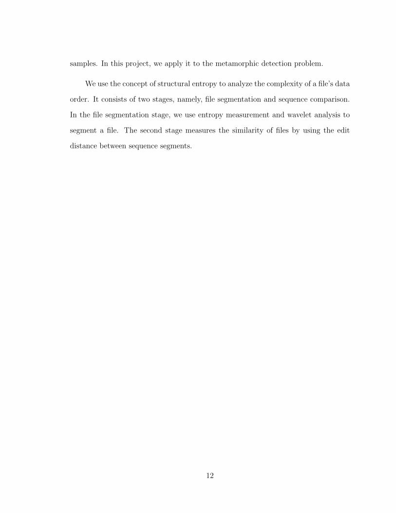
In this project, we use the concept of structural entropy to analyze variations in

the complexity of data within a file. The process consists of two stages, namely, file

segmentation and sequence comparison. In the file segmentation stage, we use entropy

measurements and wavelet analysis to segment a file. The second stage measures the

similarity of files by computing the edit distance between sequence segments. We

apply this technique to the metamorphic detection problem and show that we can

obtain strong results in certain challenging cases.

ACKNOWLEDGMENTS

My sincere appreciation is due to my advisor, Dr. Mark Stamp, for his guidance

and encouragement throughout the project. I consider it an honor to have worked

with a professor who possesses true passion for teaching.

I would like to thank my committee members, Dr. Robert Chun and Dr. Richard

Low, for their contribution in the completion of this project.

I would like to express my earnest love and gratitude to my husband, Mark, for

his unconditional support and understanding through the duration of my studies. A

special recognition goes to my 2-year old daughter, Olivia, who keeps my work-life

balance in-check. Finally, I would like to thank my mom, Cynthia, for her continued

support and praises.

v

TABLE OF CONTENTS

CHAPTER

1 Introduction . . . . . . . . . . . . . . . . . . . . . . . . . . . . . . . . 1

2 Background . . . . . . . . . . . . . . . . . . . . . . . . . . . . . . . . 3

2.1 Malware . . . . . . . . . . . . . . . . . . . . . . . . . . . . . . . . 3

2.1.1 Viruses and worms . . . . . . . . . . . . . . . . . . . . . . 4

2.1.2 Obfuscation techniques . . . . . . . . . . . . . . . . . . . . 4

2.2 File similarity methods . . . . . . . . . . . . . . . . . . . . . . . . 7

2.2.1 HMM-based detection . . . . . . . . . . . . . . . . . . . . 7

2.2.2 Similarity index . . . . . . . . . . . . . . . . . . . . . . . . 9

2.2.3 Opcode graph-based similarity . . . . . . . . . . . . . . . . 10

2.3 Structural entropy . . . . . . . . . . . . . . . . . . . . . . . . . . . 11

3 Design . . . . . . . . . . . . . . . . . . . . . . . . . . . . . . . . . . . 13

3.1 File segmentation . . . . . . . . . . . . . . . . . . . . . . . . . . . 13

3.1.1 Wavelet transform analysis . . . . . . . . . . . . . . . . . . 14

3.1.2 Segmentation using wavelet transform . . . . . . . . . . . . 15

3.2 Sequence comparison . . . . . . . . . . . . . . . . . . . . . . . . . 18

3.2.1 Levenshtein distance . . . . . . . . . . . . . . . . . . . . . 18

3.2.2 Sequence alignment using Levenshtein distance . . . . . . . 19

3.2.3 Similarity calculation . . . . . . . . . . . . . . . . . . . . . 22

4 Experiments . . . . . . . . . . . . . . . . . . . . . . . . . . . . . . . . 24

4.1 Test data . . . . . . . . . . . . . . . . . . . . . . . . . . . . . . . . 25

vi

vii

4.2 Parameters . . . . . . . . . . . . . . . . . . . . . . . . . . . . . . . 26

4.3 Results . . . . . . . . . . . . . . . . . . . . . . . . . . . . . . . . . 27

5 Conclusion and Future Work . . . . . . . . . . . . . . . . . . . . . 36

APPENDIX

A MWOR Results . . . . . . . . . . . . . . . . . . . . . . . . . . . . . 41

B NGVCK Results . . . . . . . . . . . . . . . . . . . . . . . . . . . . . 45

C ROC Curves . . . . . . . . . . . . . . . . . . . . . . . . . . . . . . . . 47

LIST OF TABLES

1 An example of instruction transposition . . . . . . . . . . . . . . . . . 6

2 Edit matrix for strings “eleven” and “elevated” . . . . . . . . . . . . 20

3 Cygwin files from ./cygutils . . . . . . . . . . . . . . . . . . . . . . . 25

4 Linux system files . . . . . . . . . . . . . . . . . . . . . . . . . . . . 26

5 MWOR 0.5 similarity statistics . . . . . . . . . . . . . . . . . . . . . 29

6 MWOR similarity statistics . . . . . . . . . . . . . . . . . . . . . . . 30

7 AUC of NGVCK . . . . . . . . . . . . . . . . . . . . . . . . . . . . . 33

viii

LIST OF FIGURES

1 “Do-nothing” instructions [29] . . . . . . . . . . . . . . . . . . . . . . 7

2 Generic Hidden Markov Model [20] . . . . . . . . . . . . . . . . . . . 8

3 Similarity index [28] . . . . . . . . . . . . . . . . . . . . . . . . . . . 10

4 Transform assembly instructions to weighted directed opcode graph [15] 11

5 Basic executable file format . . . . . . . . . . . . . . . . . . . . . . . 14

6 Wavelet and signal under investigation [1] . . . . . . . . . . . . . . . 15

7 File segmentation process . . . . . . . . . . . . . . . . . . . . . . . . 16

8 Entropy plot of a sample file . . . . . . . . . . . . . . . . . . . . . . . 17

9 Wavelet transform of a sample file . . . . . . . . . . . . . . . . . . . . 17

10 Penalty cost for the entropy difference between two segments . . . . . 21

11 Sequence comparison process . . . . . . . . . . . . . . . . . . . . . . . 23

12 G2 similarity . . . . . . . . . . . . . . . . . . . . . . . . . . . . . . . 28

13 MWOR 0.5 similarity . . . . . . . . . . . . . . . . . . . . . . . . . . . 29

14 NGVCK (4 KB) similarity . . . . . . . . . . . . . . . . . . . . . . . . 31

15 NGVCK (8 KB) similarity . . . . . . . . . . . . . . . . . . . . . . . . 32

16 NGVCK (4 KB and 8 KB) similarity . . . . . . . . . . . . . . . . . . 32

17 NGVCK ROC curves . . . . . . . . . . . . . . . . . . . . . . . . . . . 33

18 AUC for NGVCK with various parameter values . . . . . . . . . . . . 34

19 File processing time . . . . . . . . . . . . . . . . . . . . . . . . . . . . 35

ix

CHAPTER 1

Introduction

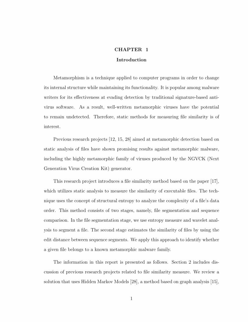
Metamorphism is a technique applied to computer programs in order to change

its internal structure while maintaining its functionality. It is popular among malware

writers for its effectiveness at evading detection by traditional signature-based anti-

virus software. As a result, well-written metamorphic viruses have the potential

to remain undetected. Therefore, static methods for measuring file similarity is of

interest.

Previous research projects [12, 15, 28] aimed at metamorphic detection based on

static analysis of files have shown promising results against metamorphic malware,

including the highly metamorphic family of viruses produced by the NGVCK (Next

Generation Virus Creation Kit) generator.

This research project introduces a file similarity method based on the paper [17],

which utilizes static analysis to measure the similarity of executable files. The tech-

nique uses the concept of structural entropy to analyze the complexity of a file’s data

order. This method consists of two stages, namely, file segmentation and sequence

comparison. In the file segmentation stage, we use entropy measure and wavelet anal-

ysis to segment a file. The second stage estimates the similarity of files by using the

edit distance between sequence segments. We apply this approach to identify whether

a given file belongs to a known metamorphic malware family.

The information in this report is presented as follows. Section 2 includes dis-

cussion of previous research projects related to file similarity measure. We review a

solution that uses Hidden Markov Models [28], a method based on graph analysis [15],

1

and a similarity index [28] technique. We also present background information on mal-

ware and briefly introduce the concept of structural entropy, which is the basis of our

similarity measure. Section 3 describes the design of our method. In Section 4, we

show the results of our solution when applied to the metamorphic malware detection

problem. Finally, in Section 5 we convey our conclusions and propose direction for

future work.

2

CHAPTER 2

Background

Development of methods for estimating file similarity is an important topic in

virus detection. Advanced anti-virus (AV) schemes such as emulation are often em-

ployed in conjunction with static signature-based detection to scan for more sophisti-

cated viruses that employ obfuscation techniques such as encryption, polymorphism,

and metamorphism. However, the overhead (e.g., file storage spaces and resources)

and the complexity of these techniques pose challenges to AV vendors. Additionally,

as we will discuss in Section 2.1.1, metamorphic malware may remain undetected

even under the scrutiny of code emulation and signature-based detection. One solu-

tion to these problems is static analysis of files. It defines file characteristics needed

for comparison without examining its functionality, thereby eliminating the emula-

tion process and in turn, reduces implementation difficulty. Also, it is purely based

on the analysis of different areas of a file which makes it resilient to techniques used

by malware writers to protect their code.

First, we provide background information on malware including the methods it

uses to avoid detection. Then, we review other file similarity measures which were

applied to the metamorphic malware detection problem. Then we briefly discuss the

concept of structural entropy and describe how we apply it to our similarity method.

2.1 Malware

Malware is a computer program designed to cause harm to computer systems.

It interrupts normal computer operation, destroys files by infection or deletion, steals

user information, and damages system resources such as the hard disk [25]. It enters

3

the system without user consent. Malware comes in various forms such as virus,

worm, trojan horse, and other programs created with malicious intent. In this paper,

we only consider viruses and worms.

2.1.1 Viruses and worms

A computer virus is a malware that executes itself by embedding its code to

another executable program. When the infected program executes, it, in turn, infects

other files, corrupting the host system. Thus, viruses are self-replicating programs

that cause destruction within the host machine [19, 25].

In contrast to viruses, worms do not require other executable files to cause intru-

sion. That is, they are standalone alone programs. A worm spreads itself from one

system to another on the network [25]. Worms not only have the ability to damage

its host system but also cause disruption to the computer networks.

Viruses and worms use a number of obfuscation techniques to avoid signature-

based detection. The aim is to make itself look different at each replication, making

it difficult for a scanner to find commonalities between the variants. To achieve

this, malware writers use methods such as encryption, polymorphism, and metamor-

phism [28]. In the next sections, our discussion will focus on viruses. However, these

topics also apply to computer worms.

2.1.2 Obfuscation techniques

Encryption is the simplest form of code obfuscation. The virus body is encrypted

using a key. Given that a different encryption key is used in each generation, the

virus variants will not share a common pattern necessary for signature scanning,

thereby evading detection. The virus also includes a decryptor module which decrypts

4

the virus body at execution. The decryptor is usually a simple, decrypted piece of

code that remain constant across replications [29]. Therefore, the decryptor code is

susceptible to detection.

Polymorphism is a step up to encryption, which possesses vulnerability to detec-

tion. That is, an encrypted virus carries a detectable decryptor code. A polymorphic

virus not only uses encryption to hide its virus body, it also mutates its decryptor

so that each virus variant looks different from one another [11, 29]. Therefore, no

common pattern exists that will allow signature scanners to use for identification.

However, just as malware writers use sophisticated methods to evade detection, AV

software vendors develop other means to defeat them. In conjunction with signature

scanning, AV vendors use code emulation to allow potential viruses to execute in a

protected environment. Once the virus decrypts itself within this virtual environment,

it exposes its virus body, which stays constant, to detection.

Metamorphic virus goes even further and mutates its entire virus body, making

it resistant to emulation. A virus using metamorphism changes its internal structure

in each replication while maintaining its functionality [11, 29]. A highly metamorphic

virus does not necessarily need encryption since each generation will produce a struc-

turally different code and retrieval of a common signature will be highly unlikely [19].

Therefore, encryption adds no benefit to the virus creation. As such, a well developed

metamorphic virus has the potential to remain undetected.

There are a number of techniques to create mutated virus programs. One sim-

ple method is to apply register swapping. In this approach, the code remains un-

changed except for the registers. For example, ADD EDX,0088h can be converted to

ADD EAX,0088h, i.e., the register EDX is swapped for EAX. However, register swapping

can typically be exploited by a wildcard string [12].

5

Another prevalent method used in metamorphism is equivalent instruction sub-

stitution. An instruction or a set of instructions is exchanged for another yielding

the same result. For example, the sequence of instructions PUSH R1; MOV R1,R2 can

be substituted for PUSH R1; PUSH R2; POP R1, which results in the same function-

ality [28].

In some instances, the order of instructions can be rearranged without losing the

functionality if the instructions have no dependency with each other. This technique

is called instruction transposition; it enables viruses avoid signature-based detection

since the order of bytes deviates in each replication [19]. A simple example of this

method is shown in Table 1.

Table 1: An example of instruction transposition

Original Instructions Transposed Instructions1: SUB R1, R2 1: SUB R3, R4

2: SUB R3, R4 2: SUB R1, R2

Subroutine permutation is another technique for manipulating the internal struc-

ture of a virus without changing the functionality. With n subroutines in a virus,

n! variants of the virus can be generated. A virus with 10 subroutines, like the

Win32/Ghost virus, can easily generate 10! or 3, 628, 800 versions of itself [29]. How-

ever, since the subroutines do not change, using this method alone can expose the

virus to detection by searching for common short string patterns [28].

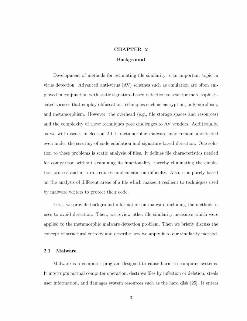
Garbage instruction insertion is an effective metamorphic technique. Garbage

instructions are those that are either executed without impacting the virus behavior,

or skipped all together. The former type of garbage instructions are often referred

as “do-nothing” code, and the latter are “dead-code” instructions. An example of a

6

“do-nothing” code sequence is shown in Figure 1.

Figure 1: “Do-nothing” instructions [29]

2.2 File similarity methods

In this section, we review previous research projects designed for estimating file

similarity between samples from a number of metamorphic family of viruses.

2.2.1 HMM-based detection

A hidden Markov model (HMM) represents a system having a Markov process in

which the states are non-observable [9, 20]. In other words, the process of transitioning

from one state to the next is dependent only on the current state and each state in

the transition sequence is hidden. What is visible, however, is the series of output

observed during the transition process [20, 28]. Figure 2 shows a generic HMM.

Here, the Markov process consists of Xt hidden states which are “driven” by the

state transition probabilities A. Each hidden state uncovers some information, i.e.,

observation Ot, over a probability distribution B. Therefore, given a sufficient sample

of observations, we can produce a model that represent the data sample maximally.

7

Figure 2: Generic Hidden Markov Model [20]

We can then determine if another given set of data is related to the observed data

represented by the model. Generating a system that models a sample data set and

utilizing it to expose data relationships are two of the three fundamental problems

that can be solved using HMMs [20]. We can also discover the unknown states of the

HMM given the model and a set of data. For more details on HMM, refer to [20].

The paper [28] presents a detector based on hidden Markov models (HMM) and

shows superiority over popular commercial virus scanners on a set of test files. The

HMM method effectively detects metamorphic viruses produced by various metamor-

phic generators including NGVCK, which generates highly morped versions of a given

virus. The technique involves training and detection phases. The training phase gen-

erates a hidden Markov model on a given file set of a metamorphic virus family (e.g.,

NGVCK). The model is trained on the assembly opcode sequences of the viruses.

The process starts by disassembling the virus executable files, producing assembly

opcodes, which are then concatenated into a long sequence of opcodes that is used

to build the model. The result is a model that represents the statistical profile of

the virus family. In order to classify a given file as being malicious or benign, the

resulting HMM is used to measure the log likelihood of the virus files in the test set,

which belongs to the same virus family used in the training phase. The expectation is

that the model would give high likelihood scores to these files. The same calculation

8

is performed on another set consisting of normal files and virus files from another

virus family. The goal is to clearly set distinctions between “family viruses”, “non-

family viruses”, and “normal files”. The results show that the HMM method is highly

effective at detecting family viruses, overpowering some commercial virus scanners.

2.2.2 Similarity index

The same paper [28] presents another similarity measure based on similarity

index. Although the technique is simpler, it is equally effective at detecting meta-

morphic viruses. In fact, the experiment resulted in 100% detection rate and 0%

false positive rate. Similar to the HMM approach, this method analyses the opcode

sequences of files. However, here it directly compares the opcode sequences of two

files by matching all three consecutive opcode subsequences from each, in any or-

der. For example, an opcode sequence of [add, sub, mov] from one file matches

the following sequences from another file: [sub, mov, add], [mov, add, sub], and

[sub, add, mov]. The matching subsequences are then plotted and adjusted, based

on a threshold, to cut down random matches. By reducing noise, the graph shows

a more accurate representation of the matching sequences. Figure 3 illustrates this

process. The similarity score is calculated based on the average of real matches. The

file being examined is categorized as “non-family” if it has no similarity to a randomly

chosen virus file from a known virus family. Otherwise, additional comparisons are

required between the chosen virus file and other files from the same virus family to

set a threshold. If the similarity score between the given file and the originally chosen

virus file is above the threshold, the file is deemed a “family” virus.

9

Figure 3: Similarity index [28]

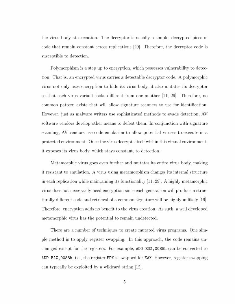
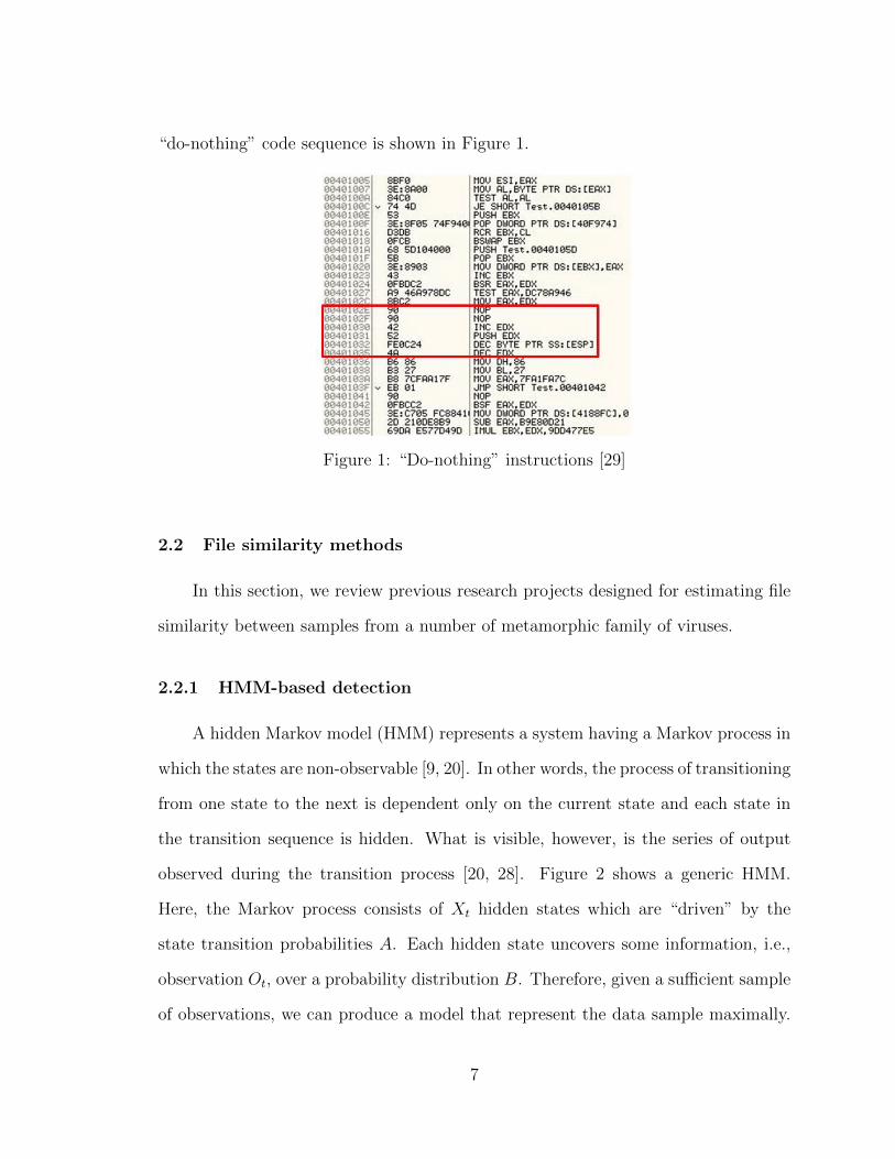
2.2.3 Opcode graph-based similarity

In a more recent work, a technique developed using opcode graph [15] outper-

forms the HMM-based detection under certain scenarios. This method takes an exe-

cutable file, disassembles it, and extracts the opcode sequence. The sequence is then

transformed into a weighted directed graph. The graph is constructed as follows. The

nodes represent all the distinct opcodes. An edge is added from each opcode node

to all of its successor opcode nodes. The probability of the successor opcode node is

assigned as the weight of the corresponding edge. Figure 4 shows an example of a

weighted opcode graph of a sample assembly instructions.

To compare two files, the opcode graph is built for each file. The generated

opcode graphs are compared directly via a scoring function which takes the corre-

sponding edge weights (probabilities of two opcodes or itself occurring in sequence)

from the two opcode diagrams and calculates a similarity score. This process is per-

formed on pairs of virus files from a metamorphic virus family. The expectation is to

get scores with little to no variations from these family viruses. Similarly, the score

10

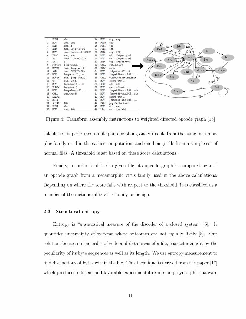
Figure 4: Transform assembly instructions to weighted directed opcode graph [15]

calculation is performed on file pairs involving one virus file from the same metamor-

phic family used in the earlier computation, and one benign file from a sample set of

normal files. A threshold is set based on these score calculations.

Finally, in order to detect a given file, its opcode graph is compared against

an opcode graph from a metamorphic virus family used in the above calculations.

Depending on where the score falls with respect to the threshold, it is classified as a

member of the metamorphic virus family or benign.

2.3 Structural entropy

Entropy is “a statistical measure of the disorder of a closed system” [5]. It

quantifies uncertainty of systems where outcomes are not equally likely [8]. Our

solution focuses on the order of code and data areas of a file, characterizing it by the

peculiarity of its byte sequences as well as its length. We use entropy measurement to

find distinctions of bytes within the file. This technique is derived from the paper [17]

which produced efficient and favorable experimental results on polymorphic malware

11

samples. In this project, we apply it to the metamorphic detection problem.

We use the concept of structural entropy to analyze the complexity of a file’s data

order. It consists of two stages, namely, file segmentation and sequence comparison.

In the file segmentation stage, we use entropy measurement and wavelet analysis to

segment a file. The second stage measures the similarity of files by using the edit

distance between sequence segments.

12

CHAPTER 3

Design

As previously cited, the similarity method we consider here is derived from the

paper [17]. It is based upon static analysis of files using structural entropy to measure

similarity between two files. In contrast to [15, 28], this solution examines executable

files without code disassembly. Instead of analyzing opcode sequences of files, we

scan the binaries directly and observe the distinctions of each byte with respect to

one another for different areas within the files. In other words, we are only interested

in the structure, specifically, entropy and size characteristics of a file.

The proposed solution compares two given files and produces a similarity mea-

sure. It starts by splitting each file into sequence of segments of different entropy

levels using entropy and wavelet analysis, followed by aligning the two sequences

by calculating the edit distance between the sequence segments. The result is the

similarity between the two files, expressed as a percentage.

3.1 File segmentation

The key in properly segmenting a file is to locate the areas where significant

changes occur. In our method, we are looking directly into the sequence of data bytes

within an executable file. The standard structure of an executable includes informa-

tion about its code and data fragments. Figure 5 shows a basic format of a Windows

portable executable file, organized into various sections [7, 13, 14]. The format starts

with structures of different headers followed by the code and data regions. Each of

these file fragments can be characterized by the nature of information it contains. For

instance, the header sections include pointers to other areas within the file, and the

13

Figure 5: Basic executable file format

text and data sections contain the code and initialized data (i.e., initialized global

and static variables), respectively [13, 14, 16]. The method we use here is based

on the notion that variants from the same malware family will share similar code

patterns and data structures in order to preserve its malicious intent. Therefore, we

can examine not only the similarity within the headers, but more importantly, the

distinctive byte sequences within the code and data sections. We can use entropy

and size to represent each of these byte patterns and use them as bases for our file

segmentation process. Consequently, our goal is to find the borders where these areas

occur and use it to segment a file. We achieve this by using wavelet analysis on a file

represented as a series of entropy measure.

3.1.1 Wavelet transform analysis

Wavelet analysis is a process of transforming a signal (i.e., a data set) into a more

revealing and useful form. It uses wavelets, which are wavelike functions, to analyze

the raw data in different locations and for different wavelet scales [1, 21]. Figure 6

illustrates the signal and the analyzing wavelet. The transformation at a given scale

is determined based on the signal approximation and detail at the previous scale.

14

Figure 6: Wavelet and signal under investigation [1]

Scaling the wavelet smooths out the high frequency information present in the original

data. The transformed data is referred as wavelet transform, which represents the

relationship of the data and the analyzing wavelet. Mathematically, it is a convolution

of the signal and the wavelet function for a range of locations and scales [1].

3.1.2 Segmentation using wavelet transform

We use wavelet analysis to trace those areas in the file where significant changes

occur. The process is as follows. First, we apply the sliding window method to

represent the file as a series of entropy measures Y = {yi : i = 1, ..., N}, where N

is the number of windows and yi is the entropy of each window. The entropy is

calculated using Shannon’s formula [3]

yi = −m∑j=1

p(j) log2 p(j), (1)

where p(j) is the frequency of byte j within window i, and m is a number of distinct

bytes in the window. Second, the resulting entropy series Y is fed into wavelet analysis

using discrete wavelet transform

W (a, b) =1

|a|1/2N∑i=1

yiψHAAR

(ti − ba

), (2)

where a is a scaling parameter, b is a shifting parameter of the analyzing wavelet, yi

is the entropy of window i, N is the number of windows in the file, and ψHAAR is the

15

Haar wavelet function, which is defined by

ψHAAR(t) =

1, 0 ≤ t < 1/2,−1, 1/2 ≤ t < 1,0, t < 0, t ≥ 1.

The wavelet transform formula in (2) requires the scaling parameter a to be of

power of 2, i.e., an = 2n where n is the maximum scale index [26]. For example, if

we want to transform the raw data to the maximum scale of 16, equation (2) will be

iterated four times for a = 2, 4, 8, and 16 and for different locations, b, on the data.

The file segments are determined by the wavelet coefficients at the maximum scale,

where boundaries of these segments are defined by the local extrema based on a set

threshold. The file segmentation process is summarized in Figure 7.

Figure 7: File segmentation process

To illustrate our file segmentation method, consider the diagram in Figure 8,

which shows the entropy plot of a 4 KB size sample file. This entropy series is calcu-

lated using a window size and window slide size of 64 bytes and 32 bytes, respectively.

16

Figure 8: Entropy plot of a sample file

Using 32 bytes for the slide size ensures the entropy map size to be of power of 2,

which is 128 in this example. The wavelet transform of this sample file is shown in

Figure 9 with maximum scale of 16, i.e., a4 = 24. On the lower transformation scales,

Figure 9: Wavelet transform of a sample file

17

detail of changes in source data is evident, while insignificant changes are ignored at

the higher scales. Therefore, the segments are determined by the coefficients at scale

index 4. Using a threshold, we can locate the segment borders by finding peaks that

are greater than the threshold in height.

3.2 Sequence comparison

Once each file has been transformed into a sequence of segments, we compare the

two sequences and determine the degree of similarity between them. The comparison

process is as follows. First, we align the two sequences by evaluating the differences of

their respective elements. We achieve this by using an algorithm based on the Leven-

shtein distance. The result is a measure of the difference between two sequences [10].

We then use this result to estimate the similarity between the two files.

In this section, we first provide background information on the Levenshtein dis-

tance. Then we illustrate how it is used in our sequence alignment algorithm. Finally,

we discuss our method for evaluating the similarity measure.

3.2.1 Levenshtein distance

The Levenshtein distance, or edit distance, is a measure of the difference between

two sequences of data [10]. It calculates the distance by tallying the minimum number

of edit operations required to transform the first sequence into the other. The set

of edit operations are substitution, insertion, and deletion. Substitution replaces an

element from the first sequence with an element in the second sequence, insertion

adds a element into the second sequence, and deletion removes an element from the

second sequence [2, 27]. Each required edit operation adds to the overall distance. In

other words, each edit translates into a penalty. Consequently, the more the edits,

18

the higher the difference is between two sequences.

Consider an example of comparing two sequences of characters where each sub-

stitution, insertion or deletion results to a penalty of 1. The number of edit operations

required to transform the string “eleven” to “elevated” is 3,

1. eleven → elevaen, insert ‘a’

2. elevaen → elevaten, insert ‘t’

3. elevaten → elevated, substitute ‘n’ for ‘d’.

Notice that the transformation cannot be completed in fewer than three edits, there-

fore the Levenshtein distance between these two strings is 3.

Equation 3 formulates the general definition of the Levenshtein distance D(i, j)

between sequences x[1 : m] and y[1 : n] where edit penalties are determined by the

cost function δ [2].

D(i, j) =

0 if i = 0 and j = 0D(0, j − 1) + δ(λ, yj) if i = 0 and j > 0D(i− 1, 0) + δ(xi, λ) if i > 0 and j = 0D(i− 1, j − 1) if xi = yj

min

D(i, j − 1) + δ(λ, yj)D(i− 1, j) + δ(xi, λ)D(i− 1, j − 1) + δ(xi, yj)

if xi 6= yj.

(3)

Applying this definition to our previous example with δ = 1 (i.e., penalty is 1) for

each edit operation produces the edit matrix in Table 2. The last matrix element

represent the edit distance, which is 3 in our example.

3.2.2 Sequence alignment using Levenshtein distance

As discussed in the the previous section, the Levenshtein distance adds a penalty

of 1 on each edit operation applied on sequences of characters. In our method, we

19

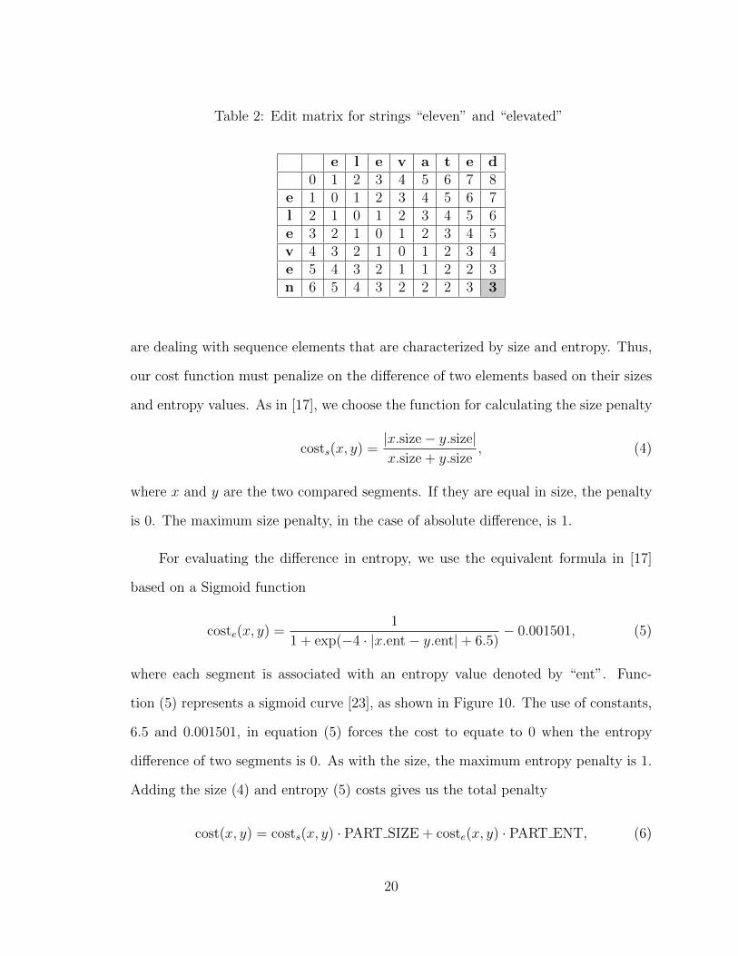
Table 2: Edit matrix for strings “eleven” and “elevated”

e l e v a t e d0 1 2 3 4 5 6 7 8

e 1 0 1 2 3 4 5 6 7l 2 1 0 1 2 3 4 5 6e 3 2 1 0 1 2 3 4 5v 4 3 2 1 0 1 2 3 4e 5 4 3 2 1 1 2 2 3n 6 5 4 3 2 2 2 3 3

are dealing with sequence elements that are characterized by size and entropy. Thus,

our cost function must penalize on the difference of two elements based on their sizes

and entropy values. As in [17], we choose the function for calculating the size penalty

costs(x, y) =|x.size− y.size|x.size + y.size

, (4)

where x and y are the two compared segments. If they are equal in size, the penalty

is 0. The maximum size penalty, in the case of absolute difference, is 1.

For evaluating the difference in entropy, we use the equivalent formula in [17]

based on a Sigmoid function

coste(x, y) =1

1 + exp(−4 · |x.ent− y.ent|+ 6.5)− 0.001501, (5)

where each segment is associated with an entropy value denoted by “ent”. Func-

tion (5) represents a sigmoid curve [23], as shown in Figure 10. The use of constants,

6.5 and 0.001501, in equation (5) forces the cost to equate to 0 when the entropy

difference of two segments is 0. As with the size, the maximum entropy penalty is 1.

Adding the size (4) and entropy (5) costs gives us the total penalty

cost(x, y) = costs(x, y) · PART SIZE + coste(x, y) · PART ENT, (6)

20

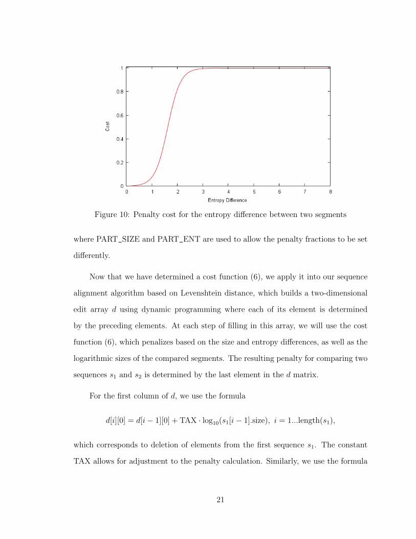
Figure 10: Penalty cost for the entropy difference between two segments

where PART_SIZE and PART_ENT are used to allow the penalty fractions to be set

differently.

Now that we have determined a cost function (6), we apply it into our sequence

alignment algorithm based on Levenshtein distance, which builds a two-dimensional

edit array d using dynamic programming where each of its element is determined

by the preceding elements. At each step of filling in this array, we will use the cost

function (6), which penalizes based on the size and entropy differences, as well as the

logarithmic sizes of the compared segments. The resulting penalty for comparing two

sequences s1 and s2 is determined by the last element in the d matrix.

For the first column of d, we use the formula

d[i][0] = d[i− 1][0] + TAX · log10(s1[i− 1].size), i = 1...length(s1),

which corresponds to deletion of elements from the first sequence s1. The constant

TAX allows for adjustment to the penalty calculation. Similarly, we use the formula

21

for filling in the first row

d[0][j] = d[0][j − 1] + TAX · log10(s2[j − 1].size), j = 1...length(s2),

which denotes insertion of elements from the second sequence s2. The rest of the

elements are set using the formula

d[i+1][j+1] = min

d[i][j] + cost(s1[i], s2[j]) · log10((s1[i].size + s2[j].size)/2)d[i][j + 1] + TAX · log10(s1[i].size)d[i+ 1][j] + TAX · log10(s2[j].size).

(7)

For each remaining item of d, we calculate the three equations in (7) and select the

minimum result. The penalty for substituting an element from s1 to an element in s2

is given by the first equation in (7). In this case, we take into account both the overall

cost (6) and the average size of the two segments. The second equation evaluates the

penalty for a deletion of an element in sequence s1. Lastly, an insertion of an element

into sequence s2 is specified by the third equation. Penalties from both the deletion

and insertion operations are based on the size of the segment.

3.2.3 Similarity calculation

Using the resulting edit distance (i.e., the last element of the edit matrix d) as

described in the previous section, we can then calculate the similarity percentage

between s1 and s2 sequences by the formula

similarity = 100− d[length(s1)][length(s2)]

costmax

× 100, (8)

where costmax is the penalty in the worst case scenario where all elements in s1 are

deleted and all elements in s2 are inserted. In addition, we increase this penalty

based on the edit operation being performed. This maximum penalty is determined

22

as follows

costmax+ =

2 · TAX · (log10(s1[i].size) + log10(s2[j].size)), s1[i] substitute s2[j]TAX · log10(s1[i].size), delete s1[i]TAX · log10(s2[j].size), insert s2[j].

(9)

Calculating costmax is similar to penalty calculations for the first column and first

row of matrix d. The only exception is the doubling of the penalty when the element

from the sequence s1 is substituted for the element in the second sequence s2.

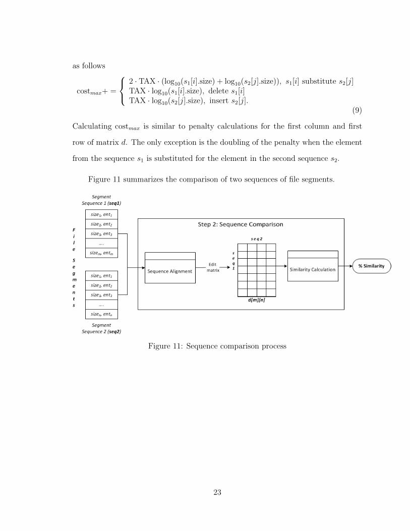
Figure 11 summarizes the comparison of two sequences of file segments.

Figure 11: Sequence comparison process

23

CHAPTER 4

Experiments

We apply our method to the metamorphic virus detection problem using a process

consistent with [15] with a slight alteration. The difference is in the number of

comparisons, i.e., pairing of files. Instead of exclusive pairing [15], we compute the

similarity of each possible pair in the test set. This progression from [15] makes for a

more complete experiment, hence produce a more accurate result.

In order to identify malicious programs, we define a similarity threshold that

separates them from the benign programs. Our goal is to clearly distinguish the

viruses from ordinary files. To set the threshold, we perform the following steps:

1. Determine the similarity range for a metamorphic virus family by calculating

the degree of similarity for all pairs of virus files. For a test set of 50 files, as in

the case of the G2 and NGVCK family of viruses, we will perform(502

)similarity

calculations, which is equivalent to 1,225 comparisons.

2. Determine the similarity range for the metamorphic files used in step 1 versus

a set of benign files by calculating the degree of similarity for all pairs. For

a set of 50 virus files and 16 benign files, this will generate (50 ∗ 16) = 800

comparisons.

3. Set the threshold by analyzing the values around the lower end of the range in

step 1 and higher end of step 2.

If a threshold can be set in step 3, then our method is capable of detecting a virus

from a known metamorphic virus family.

24

4.1 Test data

We use 50 virus files generated by G2 (Second Generation virus generator) and

50 files from the NGVCK virus family [24]. For the comparison set (i.e., benign files),

we use 16 randomly selected Cygwin utilities files [4] shown in Table 3. The Cygwin

files are chosen with the assumption that much of their functionality is comparable

with those of the virus programs without the malicious intent. The Cygwin utilities

files were also used for comparison in [15, 28].

Table 3: Cygwin files from ./cygutils

Cygwin benign file Cygwin benign fileascii.exe msgtool.exebanner.exe putclip.execonv.exe readshortcut.execygdrop.exe realpath.execygstart.exe getclip.exedump.exe semstat.exelpr.exe semtool.exemkshortcut.exe shmtool.exe

We also evaluate our method against metamorphic worms generated by

MWOR [18, 19], which is a generator developed to evade statistical-based detection

such as the HMM-based detector we discussed in Section 2.2.1. One of the metamor-

phic techniques MWOR uses is dead code insertion. The amount of dead-code added

in each replication is determined by the dead-code to worm-code padding ratio. A

padding ratio of 2 means that the dead-code is twice as much as the worm instruc-

tions. Additionally, the instructions used for padding are retrieved from a subset of

the benign files in our test set. Insertion of dead-code allows the worm to assimilate

code patterns present in benign programs. Its intent is to resemble ordinary programs

25

to avoid detection.

In our experiments, we use seven sets of MWOR with increasing padding ratios

of 0.5, 1.0, 1.5, 2.0, 3.0, and 4.0 [24]. With higher padding ratios, the expectation is

a high degree of similarity will result from worm and benign files comparison. Since

the MWOR files [24] were generated on a Linux environment, for comparison, we use

a set of 30 Linux system programs shown in Table 4.

Table 4: Linux system files

Linux benign file Linux benign file/bin/date usr/bin/kill/bin/dmesg usr/bin/killall/bin/grep usr/bin/last/bin/mknod usr/bin/ld/bin/mount usr/bin/namei/bin/rm usr/bin/nm/bin/sleep usr/bin/nm-tool/bin/sync usr/bin/objdump/bin/touch usr/bin/oclock/usr/bin/as usr/bin/readelf/usr/bin/at usr/bin/rpl8/usr/bin/file usr/bin/shuf/usr/bin/funzip usr/bin/size/usr/bin/dig usr/bin/strip/usr/bin/msgcat usr/bin/sum

4.2 Parameters

Recall that our algorithm consists of two stages, namely, file segmentation and

sequence comparison. In the file segmentation phase, we build an entropy map of a

file using sliding window. We set the window size to 64 bytes for the G2 and NVGCK

files, and 256 bytes for the MWOR file sets. The slide size is set to approximately

26

half the window size, making certain that the entropy map is of size power of 2. This

size restriction is due to the segmentation algorithm, which successively splits the

input data in half at each transformation scale [22]. We use lower values for G2 and

NGVCK due to their small file sizes. Higher parameter values generate insufficient

number of segments necessary for sequence comparison.

For computing the total penalty cost in equation (6) in the sequence compari-

son phase, we set the coefficients to 0.4 and 1.6 for PART_ENT and PART_SIZE,

respectively. By using such values, the size difference of the compared segments is

augmented. This increases the influence of the size penalty to the overall cost. The

constant TAX is set to 0.3, meaning the average penalty for a pair of mismatching

segments is 0.3.

4.3 Results

First, we applied our similarity measure to a family of G2 viruses and a set of

Cygwin utility files. We used the process outlined at the start of this chapter. Fig-

ure 12 shows the results, where the red points correspond to the similarity percentages

between virus pairs and the virus-benign pairs are denoted by the green points. You

can see in this diagram that the G2 viruses are almost identical with one another.

The similarity percentages are all above 95%. Since [28] found that the virus vari-

ants generated by G2 have the highest average similarity among other generators,

the result here is as expected. Also, notice the three bands among the virus-benign

pairs. These are formed due to the file size difference between the benign files and

the viruses. The higher the size difference, the lower the similarity is between them.

Evidently, our method is capable of detecting G2 viruses with false positive rate of

0%. We can easily use the lowest similarity score of a pair of viruses for setting the

27

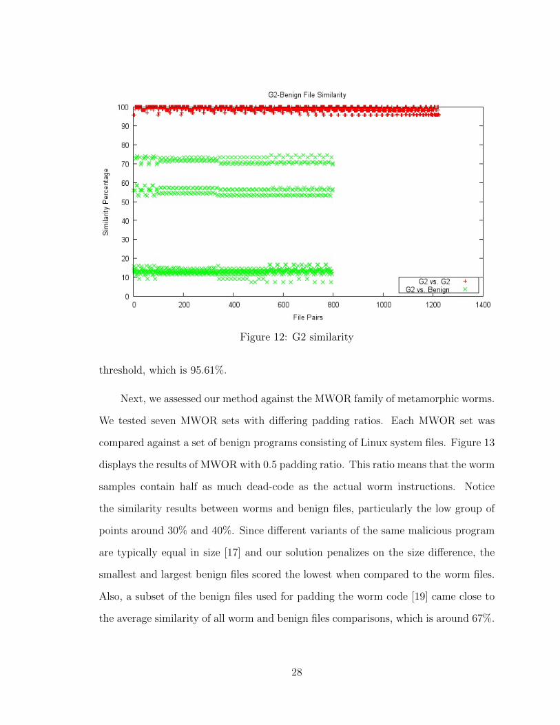
Figure 12: G2 similarity

threshold, which is 95.61%.

Next, we assessed our method against the MWOR family of metamorphic worms.

We tested seven MWOR sets with differing padding ratios. Each MWOR set was

compared against a set of benign programs consisting of Linux system files. Figure 13

displays the results of MWOR with 0.5 padding ratio. This ratio means that the worm

samples contain half as much dead-code as the actual worm instructions. Notice

the similarity results between worms and benign files, particularly the low group of

points around 30% and 40%. Since different variants of the same malicious program

are typically equal in size [17] and our solution penalizes on the size difference, the

smallest and largest benign files scored the lowest when compared to the worm files.

Also, a subset of the benign files used for padding the worm code [19] came close to

the average similarity of all worm and benign files comparisons, which is around 67%.

28

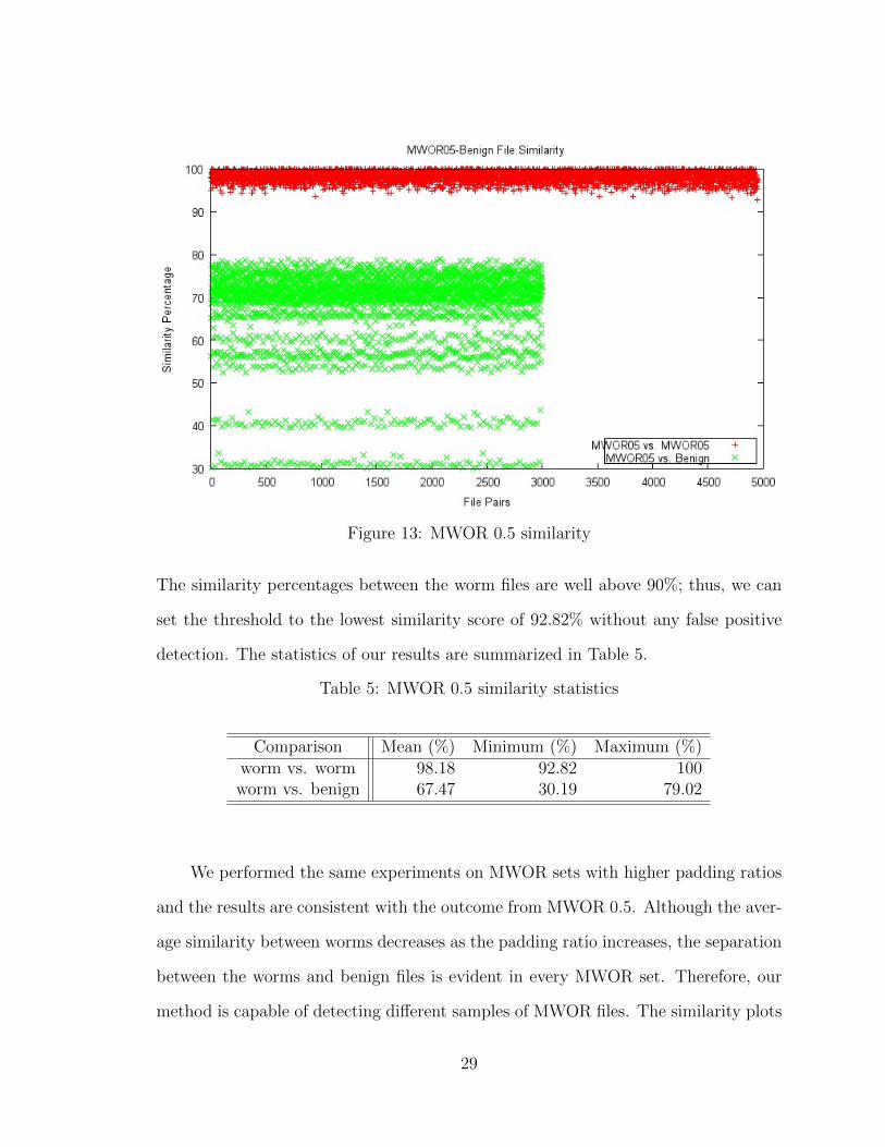
Figure 13: MWOR 0.5 similarity

The similarity percentages between the worm files are well above 90%; thus, we can

set the threshold to the lowest similarity score of 92.82% without any false positive

detection. The statistics of our results are summarized in Table 5.

Table 5: MWOR 0.5 similarity statistics

Comparison Mean (%) Minimum (%) Maximum (%)worm vs. worm 98.18 92.82 100worm vs. benign 67.47 30.19 79.02

We performed the same experiments on MWOR sets with higher padding ratios

and the results are consistent with the outcome from MWOR 0.5. Although the aver-

age similarity between worms decreases as the padding ratio increases, the separation

between the worms and benign files is evident in every MWOR set. Therefore, our

method is capable of detecting different samples of MWOR files. The similarity plots

29

are shown in Appendix A. Table 6 summarizes the similarity statistics of the MWOR

families.

Table 6: MWOR similarity statistics

Family Comparison Mean (%) Minimum (%) Maximum (%)MWOR 1.0 worm vs. worm 97.50 93.14 100.00

worm vs. benign 66.63 30.50 79.61MWOR 1.5 worm vs. worm 97.08 93.20 100.00

worm vs. benign 68.60 24.19 78.61MWOR 2.0 worm vs. worm 96.33 91.96 100.00

worm vs. benign 68.72 26.73 78.49MWOR 2.5 worm vs. worm 95.62 92.23 100.00

worm vs. benign 68.32 24.16 77.87MWOR 3.0 worm vs. worm 95.00 89.30 100.00

worm vs. benign 67.68 26.06 77.87MWOR 4.0 worm vs. worm 93.84 89.96 100.00

worm vs. benign 65.82 27.24 78.64

Lastly, we turn to the NGVCK virus family, which [28] found to be the most

highly metamorphic. Our first observation is that files in this sample differ in size.

This is unlike the G2 and MWOR test data where all the files within each set have

the same size. Out of the 50 NGVCK files in our test set, 34 files are 4 kilobytes

in size, 13 files are 8 kilobytes, and the other three files are 16, 36, and 40 kilobytes

(KB). First, we ran a similarity test between the 34 NGVCK files (4 KB) and a set

of Cygwin files listed in Table 3. The plot is shown in Figure 14. While the average

similarity score of the virus pairs came out high at 90.31%, there are a number of

overlaps among the virus and benign file comparisons. If we take the minimum score

from the virus pair comparisons and set it as the threshold, 1.5% of the virus and

benign pairs score higher than the threshold.

We repeated the same test on the group of 13 NGVCK files having equal size of

30

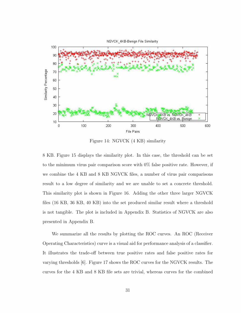
Figure 14: NGVCK (4 KB) similarity

8 KB. Figure 15 displays the similarity plot. In this case, the threshold can be set

to the minimum virus pair comparison score with 0% false positive rate. However, if

we combine the 4 KB and 8 KB NGVCK files, a number of virus pair comparisons

result to a low degree of similarity and we are unable to set a concrete threshold.

This similarity plot is shown in Figure 16. Adding the other three larger NGVCK

files (16 KB, 36 KB, 40 KB) into the set produced similar result where a threshold

is not tangible. The plot is included in Appendix B. Statistics of NGVCK are also

presented in Appendix B.

We summarize all the results by plotting the ROC curves. An ROC (Receiver

Operating Characteristics) curve is a visual aid for performance analysis of a classifier.

It illustrates the trade-off between true positive rates and false positive rates for

varying thresholds [6]. Figure 17 shows the ROC curves for the NGVCK results. The

curves for the 4 KB and 8 KB file sets are trivial, whereas curves for the combined

31

Figure 15: NGVCK (8 KB) similarity

Figure 16: NGVCK (4 KB and 8 KB) similarity

32

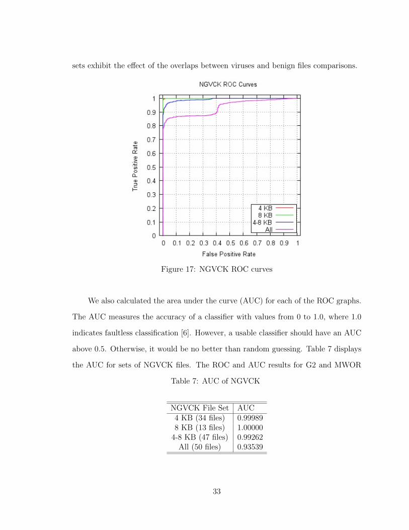
sets exhibit the effect of the overlaps between viruses and benign files comparisons.

Figure 17: NGVCK ROC curves

We also calculated the area under the curve (AUC) for each of the ROC graphs.

The AUC measures the accuracy of a classifier with values from 0 to 1.0, where 1.0

indicates faultless classification [6]. However, a usable classifier should have an AUC

above 0.5. Otherwise, it would be no better than random guessing. Table 7 displays

the AUC for sets of NGVCK files. The ROC and AUC results for G2 and MWOR

Table 7: AUC of NGVCK

NGVCK File Set AUC4 KB (34 files) 0.999898 KB (13 files) 1.00000

4-8 KB (47 files) 0.99262All (50 files) 0.93539

33

are in Appedix C.

Additionally, to analyze the impact of the cost parameters, we calculated the

AUC for different values of PART_ENT and PART_SIZE on the complete NGVCK

file set. For the entropy parameter, we used a range of values from 0 to 1 with

0.05 increments, and values from 0 to 2 with 0.10 increments for the size parame-

ter. Figure 18 shows the results. Notice that for any values of PART_ENT where

PART_SIZE is below 0.80 and for any combination where PART_ENT is below 0.25,

our method’s accuracy is 0.92 at best, which is lower than our experimental result

found in Table 7 for all 50 NGVCK files. This confirms that the parameter values

used in our experiments are adequate.

Figure 18: AUC for NGVCK with various parameter values

Finally, to determine the efficiency of our method, we processed various files with

sizes ranging from 10 KB to 4 MB. For files less than 100 KB in size, the processing

34

time is around 0.02 seconds. A 4 MB file took less than 1 second to complete. The

results are shown in Figure 19. Note that the largest malware file in our experiments

is 68 KB, so each of those samples took no longer than 0.02 seconds to score. These

processes times were measured on a 64-bit Windows 7 machine with Intel Core i5-

2540M processor at 2.60 GHz and 8 GB of memory.

Figure 19: File processing time

35

CHAPTER 5

Conclusion and Future Work

The similarity method presented in this paper is based on static analysis of

files. Development of such measure is vital in classification of highly metamorphic

malware since it uses obfuscation techniques designed to evade signature-based de-

tection. We reviewed other static detection schemes, which analyze opcode sequences

of executable files. In contrast, our solution examines the binary files directly and

evaluates the distinction of bytes within the files. Therefore, our algorithm requires

no code disassembly, reducing computational overhead.

We applied our method to the metamorphic malware detection problem. The ex-

periments show that our proposed solution is capable of identifying malware samples

generated by the G2 and MWOR metamorphic generators at a 100% rate. It appears

that the amount of dead-code applied by the MWOR generator in our test set did not

impact the structural entropy of the worms. However, it is valuable to mention that

the average similarity between MWOR files slowly decreased with increasing padding

ratio. Therefore, given a sufficient amount of dead-code may strengthen its ability

against static detection. Nevertheless, large blocks of instructions that never execute

may appear suspicious to modern anti-virus emulators.

We repeated the same experiment against NGVCK family of viruses. Imme-

diately, we noticed the size differences of the NGVCK files, 34 of which are 4 KB

in size, 13 are 8 KB, and the other three files are 16 KB, 36 KB, and 40 KB. We

grouped these files based on their sizes and ran separate tests. We also ran additional

tests on combined files. Our technique was able to distinguish the viruses from the

36

benign programs with a tolerable 1.5% false match for the 4 KB files. The 8 KB

NGVCK files resulted in 100% detection rate without false positive. In the combined

test, however, a threshold was not viable. Our experiments resulted in a number of

overlaps between viruses and benign files. It appears that NGVCK not only has the

ability to change its structure at certain generations, it also makes some variants look

more like normal programs.

Overall, our results indicate that a similarity measure based on structural entropy

is potentially useful for classifying highly metamorphic malware. At the least, this

creates an additional hurdle that a malware writer must clear to create metamorphic

malware that is undetectable by static means.

For future work, it might be worthwhile to further study the NGVCK samples

and its morphing techniques. Also, it may be worth exploring the cost function used

this research. Balancing the influence of the entropy and size differences between

compared elements might improve the similarity score. Furthermore, consideration

of other algorithms for sequence comparison that employ local alignment may also

improve the results for sequences with diverse lengths, which is the case for the

NGVCK samples. Such alignment methods take into account only similar regions

rather than all elements in the sequences. A well-known method based on local

sequence alignment is the Smith-Waterman algorithm, which compares all possible

sub-sequences and selects the optimal one [30].

37

LIST OF REFERENCES

[1] P. Addison. The Illustrated Wavelet Transform Handbook: Introductory Theoryand Applications in Science, Engineering, Medicine and Finance. Taylor andFrancis Group, 2002.

[2] A. Apostolico and Z. Galil. Pattern Matching Algorithms. Oxford UniversityPress, 1997.

[3] M. Borda. Fundamentals in Information Theory and Coding. Springer, 2011.

[4] Cygwin. Cygwin utility files.http://www.cygwin.com/.

[5] Dictionary, Entropy.http://dictionary.reference.com/browse/entropy.

[6] T. Fawcett. ROC graphs: notes and practical considerations for researchers.Bioinformatics and Computational Biology, George Mason University, 2004.http://binf.gmu.edu/mmasso/ROC101.pdf.

[7] R. Islam, A. W. Naji, A. A. Zaidan, and B. B. Zaidan. New system for securecover file of hidden data in the image page within executable file using statis-tical steganography techniques. International Journal of Computer Science andInformation Security (IJCSIS), Vol. 7, No. 1, pp. 273-279, January 2010.

[8] Karmeshu. Entropy Measures, Maximum Entropy Principle and Emerging Ap-plications. Springer, 2003.

[9] S. Kazi, Hidden markov models for software piracy detection, Master’s report,Department of Computer Science, San Jose State University, 2012.http://scholarworks.sjsu.edu/etd_projects/236/.

[10] Wikipedia. Levenshtein distance, 2012.http://en.wikipedia.org/wiki/Levenshtein_distance.

[11] SearchSecurity. Metamorphic and polymorphic malware, 2010.http://searchsecurity.techtarget.com/definition/

metamorphic-and-polymorphic-malware.

[12] M. Patel, Similarity tests for metamorphic virus detection, Master’s re-port, Department of Computer Science, San Jose State University, 2011.http://scholarworks.sjsu.edu/etd_projects/175/.

38

[13] M. Pietrek. Peering inside the PE: a tour of the Win32 portable executable fileformat. MSDN Magazinehttp://msdn.microsoft.com/en-us/magazine/ms809762.aspx.

[14] S. Robinson. Expert .NET 1.1 Programming. Apress, 2004.

[15] N. Runwal, R. Low, and M. Stamp, Opcode graph similarity and metamorphicdetection. Journal in Computer Virology, Vol. 8, No. 1-2, pp. 37-52, May 2012.

[16] A. Singh. Identifying Malicious Code Through Reverse Engineering. Springer,2009.

[17] I. Sorokin. Comparing files using structural entropy. Journal in Computer Virol-ogy, Vol. 7, No. 4, pp. 259-265, November 2011.

[18] S. M. Sridhara. Metamorphic worm that carries its own morphing engine. Mas-ter’s report, Department of Computer Science, San Jose State University, 2012.http://scholarworks.sjsu.edu/etd_projects/240/.

[19] S. M. Sridhara and M. Stamp. Metamorphic worm that carries its own morphingengine. Journal in Computer Virology, October 2012.

[20] M. Stamp, A revealing introduction to hidden Markov models, 2012,http://cs.sjsu.edu/~stamp/RUA/HMM.pdf.

[21] Z. Struzik and A. Siebes. The haar wavelet transform in the time series similarityparadigm. In Proceedings of the Third European Conference on Principles ofData Mining and Knowledge Discovery (PKDD ’99). Springer-Verlag, London,UK, 12-22.http://dl.acm.org/citation.cfm?id=669368.

[22] P. Van Fleet, The discrete haar wavelet transformation, Joint MathematicalMeetings, Center for Applied Mathematics, University of St. Thomas, 2007,http://cam.mathlab.stthomas.edu/wavelets/pdffiles/

NewOrleans07/HaarTransform.pdf.

[23] G. Verschuuren. Excel 2007 for Scientists and Engineers. Holy Macro! Books,2008.

[24] Department of Computer Science, San Jose State University. Virus files, 2012.http://cs.sjsu.edu/~stamp/viruses/.

[25] Symantec. Viruses, worms, and trojans, 2011.http://service1.symantec.com/support/nav.nsf/docid/1999041209131106.

39

[26] T. Vuorenmaa, The discrete wavelet transform with financial time seriesapplications, Seminar on Learning Systems, University of Helsinki, 2003.http://www.rni.helsinki.fi/teaching/sols/TV_RNI.pdf.

[27] R. A. Wagner and M. J. Fischer. The string-to-string correction problem. Journalof the ACM (JACM), Vol. 21, No. 1, pp. 168-173, January 1974.

[28] W. Wong and M. Stamp, Hunting for metamorphic engines. Journal in ComputerVirology, Vol. 2, No. 3, pp. 211-229, December 2006.

[29] I. You and K. Yim, Malware obfuscation techniques: a brief survey. Broadband,Wireless Computing, Communication and Applications (BWCCA), 2010 Inter-national Conference on, pp. 297-300, November 2010.

[30] M. Zvelebil and J. O. Baum. Understanding Bioinformatics. Garland Science,Taylor & Francis Group, 2008.

40

APPENDIX A

MWOR Results

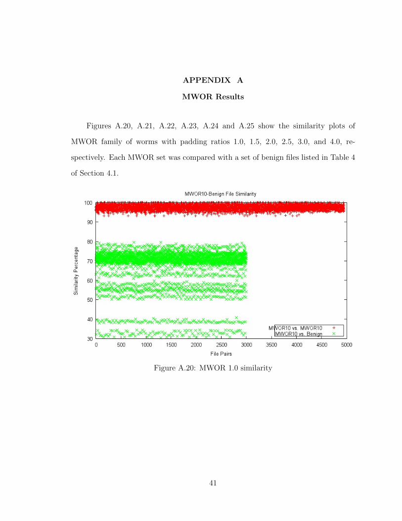
Figures A.20, A.21, A.22, A.23, A.24 and A.25 show the similarity plots of

MWOR family of worms with padding ratios 1.0, 1.5, 2.0, 2.5, 3.0, and 4.0, re-

spectively. Each MWOR set was compared with a set of benign files listed in Table 4

of Section 4.1.

Figure A.20: MWOR 1.0 similarity

41

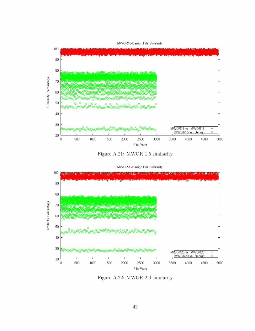
Figure A.21: MWOR 1.5 similarity

Figure A.22: MWOR 2.0 similarity

42

Figure A.23: MWOR 2.5 similarity

Figure A.24: MWOR 3.0 similarity

43

Figure A.25: MWOR 4.0 similarity

44

APPENDIX B

NGVCK Results

Figure B.26 shows the similarity plot for all 50 NGVCK files. The statistics for

the NGVCK sets are in Table B.8.

Figure B.26: NGVCK similarity

45

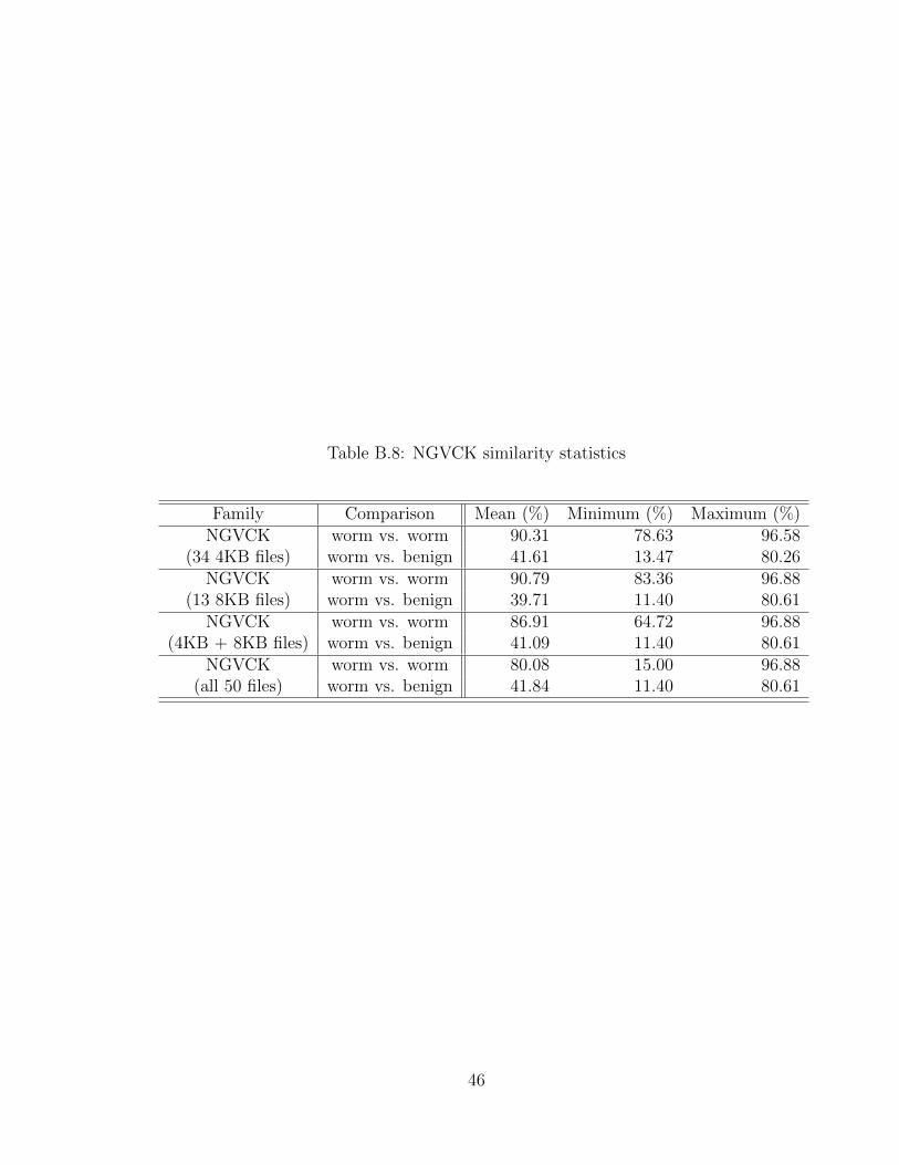
Table B.8: NGVCK similarity statistics

Family Comparison Mean (%) Minimum (%) Maximum (%)NGVCK worm vs. worm 90.31 78.63 96.58

(34 4KB files) worm vs. benign 41.61 13.47 80.26NGVCK worm vs. worm 90.79 83.36 96.88

(13 8KB files) worm vs. benign 39.71 11.40 80.61NGVCK worm vs. worm 86.91 64.72 96.88

(4KB + 8KB files) worm vs. benign 41.09 11.40 80.61NGVCK worm vs. worm 80.08 15.00 96.88

(all 50 files) worm vs. benign 41.84 11.40 80.61

46

APPENDIX C

ROC Curves

Figure C.27 shows the ROC curve for G2 with AUC of 1.0. The results from the

MWOR experiments all produced the same ROC curve, which is shown in Figure C.28

with AUC of 1.0.

Figure C.27: G2 ROC curve

47

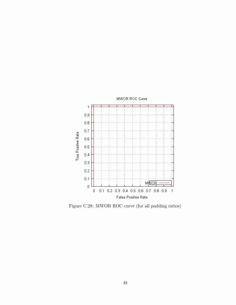
Figure C.28: MWOR ROC curve (for all padding ratios)

48