structural dynamic model updating using eigensensitivity analysis
TRANSCRIPT

IMPERIAL COLLEGE OF SCIENCE, TECHNOLOGY
AND MEDICINE
(University of London)
STRUCTURAL DYNAMIC
MODEL UPDATING
USING
EIGENSENSITIVITY ANALYSIS
bY
Haeil Jung
A thesis submitted to the University of London for the degree of
Doctor of Philosophy.
Department of Mechanical Engineering
Imperial College, London SW7, U.K.
January 1992
_’ , I._., ri .., ~-_- 1

i
ABSTRACT
Despite the highly sophisticated development of finite element methods, a finite element
model for structural dynamic analysis can be inaccurate or even incorrect due to the
difficulties of correct modelling, uncertainties on the finite element input data and
geometrical oversimplification, while the modal data extracted from measurement are
supposed to be correct, even though incomplete. Therefore, model updating schemes are
developed which aim to improve or to correct the initial finite element model using modal
test results.
In this thesis, the advantages and disadvantages (or limitations) of various model
updating methods are discussed. One of the advantages of model updating using
eigensensitivity analysis is that mode expansion is not required. However, this method
requires large computational effort because of the repeated solution of the eigendynamic
problem and repeated calculation of the sensitivity matrix. A sensitivity method is
developed using arbitrarily chosen macro elements in this thesis at the error location stage
in or&r to reduce the computational time and to reduce the number of experimental modes
required By this approach, the model updating problem which is generally under-
determined can be transformed into an over-determined one and the updated analytical
model can be a physically meaningful model.
The assumption that the test results represent the true dynamic behaviour of the structure,
however, may not be correct because of various measurement errors. The errors involved
in modal parameter estimation are investigated and their effects on estimated frequency
response functions(FRFs) and on the modal parameters extracted from the FRFs are also
investigated. The resultant ‘experimental’ modal data which contain possible experiintal
errors are used to update &corresponding analytical model to check the validity of the

ii
updating method developed. Also, the sensitivity of the updating method to noise on the
experimental data is investigated.

. . .111
ACKNOWLEDGMENTS
The author is most grateful to his supervisor, Prof. D.J. Ewins, for his sustained
stimulus and guidance throughout the duration of this research and for his sustained
advice in the preparation of the manuscript.
Many members of the Dynamic Section have helped with practical advice and discussion
of experimental and computing problems. Special thanks are due in this regard to Mr.
D.A. Robb and Dr. M. Imregun. .
For their friendly cooperation and useful discussions throughout the duration of this
work, the author also wishes to express his gratitude to many former and present
colleagues in the Dynamic Section, especially to R. Lin, A. Nobari and Y. Ren.
Finally, the author is indebted to Kia Motors Corporation for providing the financial
support throughout the whole period of this work.
t ,. ,

iV
NOMENCLATURE
As this thesis embraces several different branches of dynamics, there is a certain amount
of overlap between the symbols normally employed in the different branches. Therefore,
most symbols are defined where they occur in the text, and only the most important of
these are listed below.
A
ai
a,Ar
a,bib7
C
Ci
d
IPli
D”le
E
ej
f(t)
f*
f*
cross-sectional area
mass correction coefficient of the irh element
measured acceleration
modal constant of the rth mode
true acceleration
stiffness correction coefficient of the izh element
complex stiffness correction coefficient of the ith element
viscous damping coefficient
damping correction coefficient of the ith element
structural damping
diameter of a push rod (Appendix D)
structural damping matrix of the ith element
updated structural damping matrix
superscript for element matrix
Young’s modulus
sensitivity coefficient
actual force applied to the structure
natural frequency of the first axial mode
analytical natural frequency

V
fb natural frequency of the first bending mode
fm upper limit of measured frequency range
fx experimental natuml frequency
G, (o ) autespectmm of measured acceleration a(t)
G,(U) cross-spectrum between measured force f(t) and measured acceleration a(t)
GAO) autcqectrum of measured force f(t)
H(o) frequency response function
H 1 ,Hz FRF estimates
i imaginary unit (= 47)
I area moment of inertia
n identity matrix
k stiffness
k, axial stiffness of a push rod
kb bending stiffness of a push rod
[Kl stiffness matrix
[I<,1 analytical stiffness matrix
IKali axial stiffness matrix of the irh element
[KbIi bending stiffness matrix of the ith element
[KTi stiffness matrix of the ith element
[Kli stiffness matrix of the ith txncm element
&II updated analytical stiffness matrix
[K*] complex stiffness matrix
[AK] stiffness error matrix
1 number of selected elements
L number of macro elements
length (Appendix B and Appendix D)
m effective mass of that part of the structure to which the accelerometer is mounted
m number of measured modes
ma accelerometermass

vi
n
“i
N
%
“1
ro1
P
(PI
UPI
UP’)
PI
[SOI
[S'l
t
T
U
u(t)
ui(t)
WIvi(t)
M
shaker mass
minimum number of measured modes
mass matrix
analytical mass matrix
mass matrix of the ith element
mass matrix of the ith macro element
updatedanalyticalmassmati
maSSt?IIWIlXUliX
number of measured coordinates
number of elements in the irh macro element
number of DoFs of a analytical model
number of averages
number of modes us& for calculation of eigenvector sensitivity
null matrix
output force from the shaker
correction coefficient vector
difference vector of correction coefficients (whole elements)
difference vector of correction coefficients (selected elements)
balanced sensitivity matrix (whole elements)
unbalanced sensitivity matrix (whole elements)
balanced sensitivity matrix (selected elements)
time
recod length
subscript for updated data
rectangular window
displacements in x direction
left singular vector matrix
displacements in y direction
right sing@ar vector matrix

vii
!!!!a
.
w(t)
waX
X
Y
a(@
Yw(A)
Harming window
window spectrum
horizontalaxis
subscript for experimental data
vertical axis
=Wtance
coherence function
difference vector between experimental and analytical modal parameters
phase angle
mass normalised eigenvector of the rth mode
mass normalised eigenvector of the rth experimental mode
difference between experimental and analytical eigenvectors of the rth mode
mass normal&d mode shape matrix
arbitrary value between zero and the first non-zero eigenvalue
Lagrange multiplier
eigenvalue for the nh
eigenvalue for the rth
mode
mode
difference between experimental and analytical eigenvalues of the rrh mode
eigenvalue matrix
experimental eigenvalue matrix
shape functions
random error of [ ]
singular value of sensitivity matrix
singular value matrix
function to be minim&I
normal&d random error of [ ]
density
modal damping of the rfh mode
measured resonance frequency

s..
VlXl
% maximum frequency
6h2 eigenvalue of the rzh mode
4 true resonance frequency
[o.$J eigenvalueof thetih mode
WI
00
Ret 1
r lHr IT[ I-'
r 1+I I
II II
*
*
A.
,
Operators and Symbols
imaginary part of a complex value
order of a value
real part of a complex value
Hermitian (complex conjugate + transpose) of a complex matrix
transposeofamatrix
inverse of a matrix
Moore-Penrose general&d inverse of a rectangular matrix
modulus
Euclidian norm of a matrix
complex conjugate
cunvolution (Chapter 5)
estimated value
derivative with respect to time
derivative with respect to displacement
Abbreviations
DFl- discrete Fourier transform
DOF degree-of-freedom
Eh4M errormatrixmethod
FE finite element

ix
fast Fourier transform
FRF frequency response function
inverse eigensensitivity method
M A C modalassuxancecriterion
SDOF single degree-of-freedom
SVD singular value decomposition

X
CONTENTS
A B S T R A C T
ACKNOWLEDGMENT
NOMENCLATURE
1.1 Structural Dynamics Analysis
1.2 Analytical Modelling - FE Analysis
1.3 Experimental Modelling - Modal Testing
1.4 Linking FE Analysis and Modal Testing
1.5 Discussion on Related Research
1.6 Preview of the Thesis
CHAPTER 1 INTRODUCTION
CHAPTER 2 MODEL UPDATING METHODS - A REVIEW
2.1
2.2
Introduction
Model Updating Methods
2.2.1 Direct Methods
2.2.1.1 Berman’s Method
2.2.2
2.2.3
2.2.1.2 Eigendynamic Constraint Method
Compatibility between Measured Modes and Analytical Model
Iteration Method - Inverse Eigensensitivity Method (IEM)
Page
i. . .Ill
iv
1
2
3
4
6
7
10
13
14
15
15
16
18
21
23
.._I..‘.,*,.. / .._ ,& .:... ,. -

xi
2.3 Error Location Methods
2.3.1 Error Matrix Method (EMM)
2.3.2 Modifkd EMM
2.3.3 IEM
2.4 Concluding Remarks
CHAPTER 3 MODEL UPDATING USING IEM 44
3.1
3.2
3.3
3.4
3.5
3.6
3.7
Preliminaries
Error Location Procedure
3.2-l Selection of Submatrices
3.2.2 Eigensensitivity
3.2.3 Compatibility between Measured Modes and Analytical Model
3.2.4 Balancing the Sensitivity Matrix
Numerical Examples
3.3.1 Influence of Choice of Macro Elements on Error Location
3.3.2 Balancing Effect
Model Updating Procedure
Application to Bay Structure
Application to the GARTEUR Structure
3.6.1 The GARTEUR Structure
3.6.2 Eigensensitivity
3.6.3 Error Location Procedure
3.6.4 Model Updating Procedure
Concluding Remarks
27
27
29
30
42
45
46
46
47
52
53
57
59
63
66
71
74
74
77
78
79
90
. .

xii
CHAPTER 4 ERROR SENSITIVITY OF THE IEM 91
4.1 Preliminaries 92
4.2 Sensitivity of IEM to Noise on Modal Parameters 93
4.2.1 Error Location Procedure 93
4.2.1.1 Sensitivity to Measurement Noise 93
4.2.1.2 Influence of Choice of Macro Elements on Error Location 95
4.2.2 Updating Procedure 95
4.3 Conclusions
C H A P T E R 5 E R R O R S INVOLVED IN MODAL PARAMETER
5.1 Preliminaries
100
5.2 Modal Testing of SAMM Structures
5.2.1 Description of Test Structures
5 . 2 . 2 M e a s u r e m e n t
5.3 Errors in Modal Parameter Estimation
5.4 Measurement Errors
5.4-l
5.4.2
5.4.3
5.4.4
5.4.5
5.4.6
Nonlinearity of Structure
Nonstationarity of Structure
Mass Loading Effect of Transducers
Errors by Transducer Characteristics
5.4.4.1 Useful Frequency Range
5.4.4.2 Transverse Sensitivity
5.4.4.3 Mounting Effect
Shaker/Structure Interaction
Measurement Noise
102
103
103
104
111
111
111
112
112
113
113
113
114
114
117
L

. . .x111
5.5 Signal Processing Errors
5.5.1
5.5.2
5.5.3
Leakage
Effect of Window Functions
Effect of Averaging
5.5.3.1 FRF Estimates
5.5.3.2 Coherence Function Estimates
5.6 Modal Analysis Errors
5.6-l Circle-Fit Modal Analysis
5.6.2 Line-Fit Modal Analysis
5.7 Numerical Case Studies
5.7.1 Mass Loading Effect
5.7.2 Shaker/Structure Interaction
5.7.3 Random Noise Effect
5.7.4 Averaging Effect
5.7.5 Leakage Error
5.8 Model Updating of Beam Structure
5.9 Conclusions
CHAPTER 6 UPDATING OF DAMPED STRUCTURES 149
6.1
6.2
6.3
6.4
Preliminaries
Complex Eigensensitivity
Application to the Bay Structure
6.3.1 Case 1 - Lightly Damped System
6.3.2 Case 2 - More Heavily Damped System
Conclusions
118
118
120
123
123
124
124
125
127
128
130
131
134
135
137
141
148
150
151
157
158
167
176

x i v
CHAPTER 7 CONCLUSIONS
7.1 General Conclusions
7.2 Contributions of’the Present Research
7.3 Suggestions for Further Work
177
178
183
185
APPENDICES 186
APPENDIX q DERIVATION OF EIGENVALUE AND EIGENVECTOR
DERIVATIVES 187
APPENDIX q ELEMENT AND MACRO MATRICES 190
APPENDIX q THE SINGULAR VALUE DECOMPOSITION 197
APPENDIX q DYNAMIC CHARAClTXISTICS OF PUSH ROD 203
APPENDIX q GENFRF USER’S GUIDE 207
APPENDIX q BENDENTMJXHOD 236
REFERENCES 241

a

01 Introduction 2 cI
CHAPTER 1
INTRODUCTION
/1.1 STRUCTURAL DYNAMICS ANALYSIS
Due to increasing demands for better performance and the use of lighter structures in
modem machinery, vibration engineers must have better testing and analysis tools than in
the past. In the automotive industry, for example, weight reduction of a vehicle has been
pursued for better fuel economy and vehicle speeds have become higher as engine
performance has been improved, both of which result in various vibration and noise
problems at high speed conditions. Yet, at the same time, requirements for reduction of
vibration and noise are also increasing.
To solve vibration and noise problems in a structure, the dynamic behaviour of the
structure needs to be understood and, subsequently, an accurate dynamic model needs to
be developed. Analyses (or predictions) of the dynamic behaviour of the structure with
such a model can reduce development cost and test effort. For example, the natural
frequencies, at which the structure can be excited into resonance motion and may cause
vibration and noise problems, calculated using the model can be used to modify the
structural design in order to reduce vibration and noise by removing the natural
frequencies outside the operating range. There are two ways of achieving a suitable
t.

Cl1 Introduction 3
dynamic model of a structure: by theoretical prediction and by experimental measurement,
respectively.
1.2 ANALYTICAL MODELLING - FE ANALYSIS
If the structure has a simple geometric shape and its physical properties are more or less
uniform throughout, then a partial differential equation of motion of the form known as
the ‘wave equation’ can be used to describe its dynamics. There are well-known solutions
to the wave equation for simple structures such as beams, shafts, shells and plates. For
complicated structures such as a vehicle body, however, these analytical approaches are
often impractical because the approximations required are too restrictive to adequately
describe their dynamics.
The requirement for a more generalised method of modelling the dynamics of large,
complicated structures with nonhomogeneous physical properties has brought about the
development of the finite element (FE) analysis. Due to advances in numerical methods
and the availability of powerful computing facilities, FE analysis has become the most
popular technique in structural dynamic analysis.
The fundamental principle of the FE method is to divide a complicated structure into many
small elements such as plates, beams, shells, etc. The mass and stiffness matrices of an
individual element, which is a simple, homogeneous element, can be obtained easily. The
global mass and stiffness matrices of the structure can be assembled using these element
matrices by considering connectivity and all the boundary conditions. Once the
mathematical model has been built (or the mass and stiffness matrices have been
constructed), the equations of motion can be solved by using various algorithms to obtain
a description of the dynamic behaviour of the structure.

cl1 Introduction 4
An FE model can be used to perform several types of analysis such as response
prediction, structural coupling, stress analysis, life time prediction, structural dynamic
modification, etc. Long before the construction of a real structure, it is possible to
investigate its dynamic behaviour using the FE model so that any deficiencies in the
design can be spotted early in the design stage where changes may cost much less than in
the later stages.
FE models, however, can be inaccurate or even incorrect due to insuffkient or inadequate
modelling detail, geometrical over-simplification and uncertainties on the finite element
input data. A survey which was carried out to assess the reliability of structural dynamic
analysis capabilities [l] showed that numerical predictions (or FE analysis) of structural
dynamic properties are not always as reliable as they are generally believed to be. This
points to a need for vibration tests on the structure in order to confirm the validity of the
FE model before it is used for detailed design analysis.
1.3
APart
EXPERIMENTAL
from the aforementioned
MODELLING - MODAL TESTING
analytical approach to develop a dynamic model for a
mechanical structure, another approach is to establish
structure by performing vibration tests and subsequent
This process is known as ‘Modal Testing’. During the
an experimental model for the
analysis on the measured data.
last two decades or so, modal
testing has developed both in theory and in practice. Many techniques have been
developed in order to extract more reliable modal parameters of structures from the test
data. These techniques have been fruitful due largely to the introduction of the fast
Fourier transform (FFT) algorithm and also to the development in recent years of
powerful multi-channel FFT analysers and to fast data acquisition equipment. The
availability of computer-controlled measurement equipment and special-purpose analysis

jTj Introduction 5
software has reduced the measurement time and human effort, and improved the
reliability and accuracy of measured data and the modal properties extracted from them.
The principle of modal testing is to vibrate a structure with a known excitation so that
natural frequencies, damping and mode shapes can be identified. There are two main
excitation methods. These are referred to as single-point excitation and multi-point
excitation (or normal mode method). The original multi-point excitation, which is the
more traditional of the two and has been used in the aerospace industry to test large
structures, attempts to excite the undamped (or normal) modes of a structure, one at a
time, while the single-point excitation approach excites the structure to vibrate in several
(all) of its modes simultaneously. There are many problems which make the multi-point
excitation method difficult, time consuming and expensive to implement. The single-point
excitation has gained much popularity in recent years because it is faster and easier to
perform and is much cheaper to implement than multi-point excitation and is being used
by many manufacturing industries, including the automotive industry. The single-point
excitation method excites a structure at one coordinate and measures the consequent
responses at all the coordinates of interest. A set of frequency response functions (FRFs)
are obtained by dividing the Fourier transforms of the response signals by the transform
of the input force. Modal parameters can be identified by performing further analysis (or
curve-fitting) on this set of FRFs.
Not only is modal testing necessary to validate an FE model, it can be applied to various
aspects. Modal testing can be used for troubleshooting vibration and noise problems in
existing mechanical structures, which might be caused either by error in the design or
construction of the structure or by wear, failure or malfunction in some of its
components. Modal testing can also be used to construct dynamic models for components
of a structure which are too difficult to model analytically.
.- . .-

01 Introduction 6
1.4 LINKING FE ANALYSIS AND MODAL TESTING
At the design stage, an analytical model - especially an FE model - can be used to predict
the vibration behaviour of a future structure and to modify the design of that structure if
any deficiencies in the design are found before the structure is constructed. At later stage,
when the structure has been constructed, modal testing can be performed to validate the
FE model. Once the model is shown to predict measured behaviour with an acceptable
accuracy, then it can be used for further analysis such as response prediction, structural
coupling, stress analysis, life time prediction, etc.. However, test results are seldom in
perfect agreement with the predictions of the FE model. Therefore the analyst and the
experimentalist are faced with the problem of reconciling two modal databases for the
same structure. Neither of these can be assumed to be perfect, but both have features
which can be combined to give a more accurate description of the dynamics of the
structure.
Because of the different limitations and assumptions implicit in the two approaches, the
FE model and experimental modal model have different characteristics and different
advantages and drawbacks. The FE model generally has a large number of coordinates so
that the vibration characteristics can be described in detail and can cover a comparatively
wide frequency range. However, due to insufficient or incorrect modelling, geometrical
over-simplification and uncertainties on the element properties (especially the properties
of joints which have not been fully explored), the FE model may well be inaccurate or
even incorrect. In contrast, the experimental data or experimentally-derived modal
properties are generally considered to be ‘correct’ or at least close to the true
representation of the structure, because modal testing deals with the actual structure rather
than an idealisation. However, due to the limited number of coordinates and modes which
can be included (because of various restrictions in measurement), the information thus
D

01 Introduction 7
obtained is available primarily as selected modal parameters, rather than the full spatial
properties as provided by the FE model.
The principle of correlating the models derived from these two different approaches is to
make use of the advantages of both and to overcome their disadvantages. Basically, it is
believed that more confidence can be placed in the experimental modal data than in the FE
model. Therefore, model updating schemes have been developed which aim to improve
or to correct the initial FE model using modal test results.
1.5 DISCUSSION OF RELATED RESEARCH
Historically, model updating has been accomplished by a “trial-and-error” approach
which was mainly dependent on the individual’s experience and intuition. With increasing
complexity of the structures involved, model updating by this means becomes more
difficult and systematic approaches are necessary. In recent years, a significant number of
methods for updating an analytical model have been developed which use test data to
identify or to improve an analytical model of a structure. One of the earliest publications is
by Rodden [2] who used test data to identify directly structural influence coefficients.
Berman et. al. [3] introduced a systematic approach in model updating: they improved an
analytical mass matrix by finding the smallest changes which make a set of measured
modes orthogonal and identified an ‘incomplete’ stiffness matrix by summing the
contributions of the measured modes and with the use of the improved mass matrix. The
stiffness matrix, however, does not resemble a true stiffness matrix. Baruch et. al. [4,5]
formulated a procedure using Lagrange multipliers for minimising changes in matrices to
satisfy specific constraints to update an analytical stiffness matrix under the assumption
that the analytical mass matrix is correct. Later, having concluded that the assumption of a
correct mass matrix is questionable, especially for a dynamic model which is often an
approximate reduced version of a much larger model [6], Berman et. al. developed a
L

cl1 Introduction 8
similar method for updating both the analytical mass and stiffness matrices [7] and
applied the method to a practical structure [8]. Variations of these methods have been
developed and investigated by Wei [9] and Caesar [lo]. The aforementioned methods do
not require iteration or eigenanalysis and the updated model possesses the ‘correct’
eigenvalues and eigenvectors. However, the modal parameters of the updated model
outside the frequency range of the experimental data remain questionable and may become
even worse than those of the original analytical model because the updated model does
not seek to preserve the connectivity of the structure [ 11,121. Another problem of those
methods is that mode expansion is essential to overcome the inevitable incompatibility
between the analytical model and the measured modes, and this may be an erroneous
procedure, thus jeopardising model updating. Ibrahim [13] developed a method which
used submatrices of system matrices as variables under the eigendynamic constraint.
Thus, the physical connectivity of the analytical model can be preserved during the
updating procedure. However, the updated model is not unique in the sense that it can be
scaled by an arbitrary factor. Later, To [12] modified Ibrahim’s meth& by using the
mass normalisation properties as another constraint to resolve the problem of uniqueness.
These two methods, however, still require mode expansion to overcome the inevitable
incompatibility between the analytical model and the measured modes.
Apart from these direct updating methods, Collins et. al. [ 141 introduced the concept of
an inverse eigensensitivity method (IEM) in an iterative procedure to update an analytical
model. Their method requires large computational effort because of the need for repeated
solution of the eigendynamic problem and repeated calculation of the sensitivity matrix (or
Jacobian matrix), especially for complicated structures with a large number of degrees of
freedom. Later, Chen et. al. [15] introduced matrix perturbation theory to calculate the
sensitivity matrix and to compute the new eigenvalues and eigenvectors. These iterative
methods do not require mode expansion and the updated model preserves the physical
connectivity. However, they do require large computational effort, and convergence is
not guaranteed if the modelling errors are not small.
c dL .

q1 Introduction 9
In addition to the methods summarised above, another approach to model updating has
been developed under the assumption that the major errors in the analytical model are
often isolated rather than distributed and thus that any attempt to update the whole
analytical model is conceptually insufficient and practically unrealistic. Sidhu et. al. [ 16)
developed the error matrix method (EMM) which aimed to locating major modelling
errors in an analytical model rather than attempting to update the whole analytical model.
Despite some advantages, this method does not succeed in locating mismodelled regions
if the number of measured modes is insufficient. And when modelling errors are not
small, this method cannot be applied because of the assumption that second- and higher-
order terms in an expansion of [K]-l-and [Ml-l can be ignored. An alternative method was
developed by He [17] to locate the modelling errors using a few measured modes
available. Unlike the case of the EMM, there is no assumption that modelling errors are
small, and error location is possible even with a very limited number of measured modes.
Similar efforts for error location are also reported in Ref. [ 181 where the method is called
‘force balance method’. The aforementioned error location methods require complete
measured coordinates, which is not practical, or mode expansion to overcome the
incompatibility between measured modes and analytical model, which, as mentioned
before, may be an erroneous procedure thus jeopardising a successful location of the
errors.
Zhang et. al. [19] employed the IEM to localise dominant error regions in an analytical
model using real eigensolutions and then updated the model by correcting the selected
parameters in an iterative calculation. As mentioned before, the IEM does not require
mode expansion and its computational time will be reduced by locating error regions first
and updating the analytical model using only the elements which are selected in error
location procedure. However, the methods suggested by Zhang have been found to be
unreliable.

01 Introduction 10
1.6 PREVIEW OF THE THESIS
The objectives of this research are to develop a reliable, sensitive and systematic method
for locating modelling errors in an analytical model using modal testing results and to
develop an updating method which can produce an improved analytical model which can
not only provide exact modal parameters measured in test but also predict correctly those
modes outside frequency range of the experimental data and at the same time can reduce
the number of experimental modes required as well as the computational time for
updating.
Various methods to correct an analytical model using modal testing results are reviewed
and their advantages and disadvantages (or limitations) are discussed in Chapter 2. All
direct methods need a mode expansion procedure to overcome the incompatibility in the
dimensions of the measured modes and the analytical model. The IEM, which is one of
iterative methods, has an advantage over direct updating methods in the sense that it does
not require a mode expansion procedure to be applied. However, convergence is not
guaranteed if the modelling errors are not small. The convergence might be improved by
locating error regions first and by correcting only the selected parameters by an iterative
calculation. In Chapter 3, a version of the IEM using arbitrarily chosen macro elements is
proposed at the error location stage in order to reduce the computational time and to
reduce the number of experimental modes required. By this approach, the model updating
problem which is generally underdetermined can be transformed into an over-determined
one. The proposed method is applied to the GARTEUR structure which is used to
represent a practical structure and to constitute a realistic problem in respect of the
incompleteness of both measured modes and coordinates.
Even though many methods have been developed in recent years for updating analytical
models for the dynamic analysis of a structure, and some of them have been proven to be
quite successful, the methods are generally based on the assumption that the test data are

ITI Introduction 11
perfect or noise-free. For any updating method to be useful for application to practical
structures, the sensitivity of the method to noise on the test data needs to be established.
In Chapter 4, typical measurement errors are introduced by contaminating the modal
parameters of the correct or modified structure with random noise of different levels and
the method proposed in Chapter 3 is applied to a bay structure for which “experimental”
data are noisy and incomplete.
The characteristics of real measurement errors might not result in random variations in the
modal parameters. For the updating method to be useful in practical application, various
error sources in testing should be considered in detail and more realistic en-or-s rather than
random noise should be introduced into the “experimental” data. In Chapter 5, various
errors involved in modal parameter estimation are examined, and their effects on
estimated FRFs and on the modal parameters extracted from the FRFs are also
investigated. The resultant “experimental” modal data which contain representative
experimental errors are used to update the corresponding analytical beam model to check
the validity of the IEM.
Measured modal data are often complex because of inherent damping in real structures
which can not be modelled by proportional damping, whereas the modal parameters of
the corresponding analytical model are real. Updating methods developed so far generally
assume that the experimental modal data are real, or postulate that the measured complex
data have successfully been converted to real data. However, the deduced real modes may
be erroneous because the experimentally-identified complex modes are : incomplete and
the deduction itself relies on the analytical model which is erroneous. In Chapter 6, a
modified version of the method suggested in Chapter 3 is developed to locate and to
update damping elements together with mass and stiffness elements in analytical model
using measured complex modal data. The proposed method is applied to the free-free bay
structure which may constitute a realistic problem in respect of the incompleteness of both
measurti modes and coordinates.

01 Introduction 12
Finally, all the new developments in this thesis are reviewed in Chapter 7 together with
suggestions for further research.


q Model Updating Methods - A Review 14
CHAPTER 2
MODEL UPDATING METHODS - A REVIEW
2.1 INTRODUCTION
One of the most important applications of modal testing is the validation of the
mathematical model for the dynamic analysis of a structure - especially a finite element
model - by comparing experimentallydetermined modal parameters with those obtained
from the analytical model. Once the analytical model is shown to predict the measured
behaviour, then it can be used with confidence for further analysis such as response
prediction, structural coupling, stress analysis, life time prediction, etc. However. due to
the difficulties of correct modelling, geometrical oversimplification and uncertainties on
the finite element input data, the analytical model could be inaccurate or even incorrect. In
contrast, modal testing is supposed to be capable of identifyimg the true modal parameters
because it deals with real structures. Therefore, model updating schemes are developed
which aim to improve or to correct the initial finite element model using modal test
results.
Historically, model updating has been accomplished by a “trial-and-error” approach
which was mainly dependent on the individual’s experience and intuition. With increasing

q M&l Updating Methods - A Review 15
complexity of the structures involved, model updating becomes more difficult and
systematic approaches are necessary.
2.2 MODEL UPDATING METHODS
In recent years, a significant number of methods for updating an analytical model have
been developed, and these can be divided into direct methods and iterative methods.
Direct methods usually require low computational effort, but the updated models do not
always constitute physically meaningful models [ 111. They tend to transform the
physically meaningful models into-representative models. On the other hand, Lerative
methods require larger computational effort because of repeated solution of the
eigendynamic problem and the pseudo-inversion of large matrices, though only some of
these will always constitute physically meaningful models if they converge [20].
In the following sxtions, the advantages and disadvantages (or limitations) of various
updating meth& will be xeviewed/summarised.
2.2.1 DIRECT METHODS
Direct updating methods seek to update a given mass matrix MA] and/or stiffness matrix
[KA] using measured eigenvalues [Ax] and eigenvectors [ax] under the equality
constraints such as eigendynamic and orthogonality properties. These methods can
themselves be categorised into two groups by the types of variables to be updated. The
first group is to use individual elements of the system matrices as variables. Another
group uses correction coefficients of element matrices as variables.
i

cl2 Model Updating Methods - A Review 16
2.2.1.1 Berman’s Method
A method for updating an analytical stiffness matrix was developed by Baruch under the
assumption that the analytical mass matrix is correct [S]. Later, Berman et. al. developed
a similar method for updating both the analytical mass and stiffness matrices [8].
Variations of these methods are given in Ref.[ lo]. The basic idea of the direct methods is
to minimise the weighted Euclidian norm between the original incorrect matrices and the
updated ones under the equality constraints.
In Berman’s method [8], an anaIytica.l mass matrix is updated first and then, based on this
updated mass matrix, the analytical stiffness matrix is updated. In his method, the
objective function to be minim&d for updating the mass matrix is
E = II mA]-lR ( [MU] - [MA] ) [MA]-‘n II
under the constraints
FI,l = MJI~ w&IT Frul Pxl = [ II
(2.1)
(2.2)
This minimisation problem can be easily solved using the method of Lagrange
multipliers. Using Lagrange multipliers, a function to be minimised may be written
Y = E + ~ ~ Xij ([~XIT [MUI [~,I - m>i=l j=l
(2.3)
Equation (2.3) is differentiated with respect to each element of l?$] and set to zero. Then
using equation (2.2) to evaluate klj yields the updated mass matrix which minimises E and
satisfies equation (2.2):
mu] = [MA] + [MA] [a,] [ma]-’ ( m - [maI ) [ma]-’ [@JT [ MA] (2.4)
L

q Model Updating Methods - A Review 17
where [ ma1 = [@,lT [ M,J [@,I
Similarly, for updating a stiftkss matrix, the objective function to be minim&d can be
definedas
e = 11 WV]-‘” ( C&l - l&l 1 [ WJI-~ 11
under the constraints
l-&II [@,I = Frul [@,I E ax2 1 9
P,lT r&J1 [@,,I = [ q2 I
l-w = [XulT
(2.5)
(2.6)
Then the updated stiffness matrix becomes:
IKul = [KAI+([AI+[AI~) (2.7)
where [A] = ; [MU][@,]([cPXJTIK,] [@,,I + [ q2 ] ) P,lTWul - WA] [@,I [@xlTIMu]
This method does not require iteration or eigenanalysis and the updated model possesses
the ‘correct’ eigenvectors and eigenvalues. However, the updated mass matrix using
Berman’s method cannot preserve the co~ectivity of the structure as shown in Refs [ 11,
121 because a connectivity constraint is not imposed. The updated stiffness matrix using
the updated mass matrix, which is not correct, also cannot be correct. As a result, the
updated model is not physically meaningful but is a representative model. Thus, the
modal parameters of the updated model outside the range of the experimental data remain
questionable and may become even worse than those of the original model. In general, an
updated model should be able to be used for further analyses. A designer is not only
interested in the correct representation of the dynamic characteristics of a structure but
often he wants to use this model for stress analysis, life time prediction, etc. Another

02 Model Updating Methods - A Review 18
problem of this method is that mode expansion is essential to overcome the inevitable
incompatibility between the analytical model and the measured modes. Various expansion
methods were investigated in Refs [21-231 but, so far, there is no expansion method
which is satisfactory for all cases.
2.2.1.2 Eigendynamic Constraint Method
As mentioned before, the physical connectivity of the analytical models should be
preserved during the updating process, and so the updated model should have the same
connectivity as that of the original model. By using correction coefficients of submatrices
of system matrices as variables instead of individual elements of system matrices, the
connectivity constraint can be easily imposed. Ibrahim [13] developed a method which
used submatrices of a system matrices as variables under the eigendynamic constraint.
However, the updated model is not unique in the sense that it can be scaled by an
arbitrary factor. The eigendynamic constraint method described below is similar to
Ibrahim’s method. However, the problem of uniqueness of the updated model was
resolved by using the mass normalisation properties of measured modes as another
constraint.
The method is formulated based on the eigendynamic equation and the mass
normalisation relationship. For the rth mode
- & [MU1 IQ,),+ [h~l~@x~r= to)~4QTMJl (~A = 1
The updated mass and stiffness matrices can be written as
(2J9
(2.9)

q Model Updating Methods - A Review 19
Flu1 =,$ aj I”lj &] = 2 bj WIjj=l
(2.10)
where 3 a.nd bj are COIT&OII factors to be determined and mlj and [KJj m submatrices
of system matrices such as
1) sub element matrices
2) Cnite element matrices
3) macro element matrices.
Substituting equation (2.10) into (2.8) results in a set of N linear algebraic equations:
[-~&I, MxL .a- -X,,[M]L,($x)r [Kl,(@,), -** [K]~z(@x)rl
(2.119
Similarly, equation (2.9) becomes
1 Combining equation (2.11) and (2.12) yields:

q Model Updating Methods - A Review 20
'0
.
.
.
0
1,
(2.13)
When there are m modes available, we can have m(N+l) linear algebraic equations:
(2.14)
If m(N+l) is greater than number of unknowns, Ll+L2, the problem becomes
overdetermined and the SVD technique can be used to solve for the unknown vector (P)
whose elements are the correction coefficients of system matrices.
This method does not require iteration or eigenanalysis and the updated model preserves
the co~ectivity of the structure. However, like other direct methods, mode expansion is
essential because of the large difference in the dimension between the measured modes
and the analytical model. The number of coordinates measured is usually one or twoI orders of magnitude smaller than that in an analytical model. As can be seen in Refs [21-
23], there is no effective expansion method so far.

q Model Updating Methods - A Review 21
2.2.2 COMPATIBILITY BETWEEN MEASURED MODES AND
ANALYTICAL MODEL
One of the main problems of model updating is that experimental modal parameters are
not directly compatible with those fkom the analytical model because:
1) the number of modes available f&n measurement (m) is usually very limited
(mea) and
2) the number of measured coordinates (n) is less than the number of coordinates
(or the number of degrees of freedom) of the analytical model (n<N).
It is practically impossible to measure all the modes because of the limitation due to the
characteristics of the experimental instruments such as accelerometers, force transducers,
signal analyser, exciter, etc. The second restriction results from the fact that vibration
measurements are too expensive to measure many coordinates and, some coordinates may
be either technically difficult to measure, such as rotations, or physically inaccessible,
such as the coordinates inside the structure.
The first restriction - incompleteness in the number of measured modes - can be resolved
by using the corresponding modes from the analytical model and omitting the unmeasured
modes which are usually the higher modes in practical situations. Therefore, there
remains the problem of the large difference in the number of coordinates between the
analytical model and measured modes. There are two possible solutions to this restriction:
1)
2)
expand the measured modes to include the unmeasured coc~dinates using an
expansion method, or
use corresponding coordinates from the analytical model and omitting the
unmeasured coordinates in model updating.

02 Model Updating Methods - A Review 22
Until recently, model reduction techniques such as that suggested by Guyan [24] or the
dynamic reduction technique [25] have been used to overcome the incompatibility.
However, because the eigenproperties are not exactly preserved in a reduced model and
the co~eztivity of the reduced model does not reflect the physical properties of the
complete analytical model, modelling errors spread into neighbouring regions [21], which
makes model updating very difficult.
The alternative to reducing the analytical model is to expand the measured mode shapes.
If mode expansion can be achieved successfully, the updating result can indicate
mismodelled elements more precisely than the approximate error regions found when
model reduction is used. Various mode expansion methods have been developed, and
comparisons between various expansion methods can be found in Refs.[22, 231. But
until now, no expansion technique can interpolate the unmeasured coordinates
satisfactorily.
The alternative approach to coping with the large difference in the number of coordinates
between the analytical model and the measured modes is to use only the corresponding
coordinates from the analytical model, omitting the unmeasured coordinates in model
updating. As can be found in updating equations (equations (2.4), (2.7), (2.13)), this
approach can not be applied to the direct methods because these methods require
compatibility of all degrees of freedom between analysis and test. One of the most
important advantages of an inverse eigensensitivity method (IEM), which will be
explained later, is that it does not require mode expansion or model reduction because it is
possible to use corresponding coordinates only.

q Model Updating Methods - A Review 23
2.2.3 ITERATION METHOD - INVERSE EIGENSENSITIVITY
METHOD (IEM)
When the measured coordinates are incomplete, measured modes must be expanded for
any direct method to be applied, which may be an erroneous procedure whichjeopardises
updating. The use of mode expansion can be avoided by using an IEM (or similar
method) where only the coordinates which have been measured in the test are used for
Updating.
Collins et. al. [14] first introduced the IEM for model updating. Later, Chen et. al. [15]
modified Collins’ method by proposing a matrix perturbation method to calculate the
sensitivity matrix and to compute the new modal parameters for the parameter estimation
The IEM uses modal parameters of an analytical model as initial values and the parameters
are updated iteratively based on the differences between the analytical and measured
values. Consider mathematically well-behaved functions fc (i=1,2,...,m) of L variables
pj, j=1,2,...,L. If we denote p as the entire vector of values pj, then in the neighbourhood
of po, the functions can be expanded in a Taylor series:
By neglecting terms of order A$ and higher, equation (2.15) can be approximated as:
L afifdP) - fi(PJ = ,: ap. *Pj
J
Inmanixform
(2.16)

02 Model Updating Methods - A Review 24
1 h(P) - fdP,)
.
.
fin(P) - LAP,)
APIAP2
.
.
.
APL
(2.17)
For a structure under study, the parameters p are to be identified and p,, are the
corresponding values used in the initial analysis. If the updated mass and stiffness
matrices are written as in equation (2.10), the number of unknowns becomes Lt+L2.
Functions fc(p) represent the measured modal parameters and fc(p,) are the
corresponding modal parameters obtained from the initial model. Equation (2.17) can beI written as:
*x1(*‘+)I
.
*L:*‘t’),
or
(A) m(n+l)xl = [sJm(n+l)x(LI+I?) (AP)(L,+&)xl
’ Aal ’...
&LlAh
.
.
.bbL2’
(2.18)
(2.19)
The elements of the sensitivity matrix [S] can be expressed as [see Appendix A]
(2.20)
k,, . _. _.._..,. i, .., ,_ _ ..;i ,, __ _

m Model Updating Methods - A Review 25
!y = c c;j(q)ji j - l
(2.2 1)
WjT ag- k*?-Cjj =
i ( X,- 5
(r4 1
- ‘zcol~a~ Ml, (r=j 1
If the number of measurd modes m is greater than (*), equation (2.19) becomes
overdetermined and the unknown vector (Ap} can be calculated by premultiplying
equation (2.19) by [S]+
(API = PI+ (A) (2.22)
wheretis the Moore-Penrose genera&d inverse. The corrections are then added to the
solution vector
IPInew = {yield + (ApI (2.23)
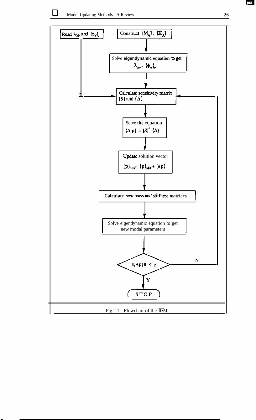
and the process is
formulated based on
be seen in Fig.2.1.
repeated iteratively to convergence because equation (2.18) is
first-order approximation. The flowchart of the whole procedure can
As explained previously, this method does not require mode expansion. In formulating
equation (2.18), it is possible to use corresponding coordinates from the analytical mode
shapes and to omit the unmeasured coordinates. The updated model will be physically
meaningful model if it converges because physical co~ectivity is preserved. However,
this method requires large computational effort because of repeated solution of the
q Model Updating Methods - A Review 26
ia
i
Solve eigendynamic equation to ge-t
A** (+*I, I
Solve the equation
(A PI = [Sl+ IAl
Update solution vector
(PLew= (PI&+ (API
I Calculate new mass and stiffhess matrices I
I Solve eigendynamic equation to getnew modal parameters
I
N
Fig.2.1 Flowchart of the EM
L

q Model Updating Methods - A Review 27
cigendynamic problem and repeated calculation of the sensitivity matrix. Also,
convergence is not guaranteed ifmodelling CrzMs are not small.
2.3 ERROR LOCATION METHODS
In addition to the methods summari sed above, another aspect of model updating is the
location of mismodelled regions before an attempt is made to improve the analytical
model. If this location is successful, then the model can be improved locally and this will
be more efficient. Any attempt to update every element in the analytical model using only
the limited information fi-om the tesi results may not be physically realistic.
2.3.1 ERROR MATRIX METHOD (EMM)
The EMM [16] aims at locating major mode&g errors in an analytical model rather than
attempting to correct the whole analytical model. The difference between correct and an
analytical stiffness matrices is defmed as stiffness error matrix [AKj
WI = [XXI - EK*l (2.24)
If [AK] is second-order in
approximated as equation
expansion of [KJl
the sense of the Euclidean
(2.25) by ignoring second
norm, theerror matrix can
and higher order terms in
- &I-9 PAI (2.25)
be
an
[Kx]-l and [KJ’can in turn be approximated using
analytical modes such that equation (2.25) becomes:
m measured and the corresponding
. ,,.
q Model Updating Methods - A Review 28
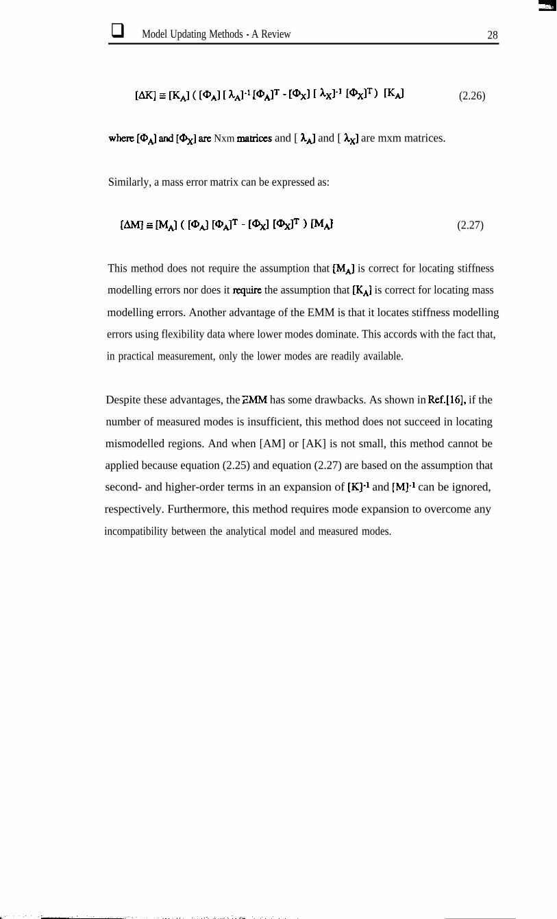
[AK] z [K*] ( [@*I [ q-1 [qJT - P&l 1 kxl-’ mclT) w (2.26)
whex [@,J and [4,J are Nxm matrices and [ X,J and [ Ix] are mxm matrices.
Similarly, a mass error matrix can be expressed as:
[AM-I = lM*l ( PA] [@*IT - [%I PXF ) lxd (2.27)
This method does not require the assumption that [MA] is correct for locating stiffness
modelling errors nor does it squire the assumption that [K,J is correct for locating mass
modelling errors. Another advantage of the EMM is that it locates stiffness modelling
errors using flexibility data where lower modes dominate. This accords with the fact that,
in practical measurement, only the lower modes are readily available.
Despite these advantages, the ZMM has some drawbacks. As shown in Ref.[l6], if the
number of measured modes is insufficient, this method does not succeed in locating
mismodelled regions. And when [AM] or [AK] is not small, this method cannot be
applied because equation (2.25) and equation (2.27) are based on the assumption that
second- and higher-order terms in an expansion of [KJ-1 and [Ml-l can be ignored,
respectively. Furthermore, this method requires mode expansion to overcome any
incompatibility between the analytical model and measured modes.

q Model Updating Methods - A Review 29
23.2 MODIFIED EMM
In consideration of the limited number of measured modes available and inconclusive
error location results, an alternative method [17] was developed to locate the modelling
errors using a few measured modes available. This method uses the product of the error
matrixandalmownmatrix:
(2.28)
Post-multiplying both sides of this equation by [%]T yields:
[ml <[qJ rqgl - VW <r@d r&l r@xn
= IMAI ([@xl Fbd [%IT) - IL1 <[@xl [%JT, (2.29)
Although error matrices cannot be obtained directly from this equation, the mismodelled
regions can be revealed explicitly by estimating the right hand side of the equation which
consists of known information. Similar efforts for error location are also reported in Ref.
[ 181 where the method is called ‘force balance method’.
Unlike the case of the EMM, there is no assumption about [W or [AK] and error location
is possible even with a very limited number of measured modes. However, this method
also requires complete measured coordinates, which is not practical, or mode expansion
to overcome the incompatibility between measured modes and analytical model, which
may be ertoneous procedure thus jeopardising exact locating, as explained before.
‘. il.,‘..,, .j / . ,l_ .: ,. .- -

q Model Updating Methods - A Review 30
2.3.3 IEM
Zhang et. al. [ 191 used the IEM to local& dominant error regions in an analytical model
using real eigensolutions and then updated the model by correcting the selected
parameters by an iterative calculation. To improve the condition of the sensitivity ma&ix
in equation (2.18), the differences in eigenvalues and corresponding rows of the
sensitivity matrix are divided by corresponding eigenvalues. Instead of solving equation
(2.22) iteratively, they suggested two erzw location methods.
A large element of the vector (Ap) represents either a dominant error region or a low
sensitivity of the corresponding element. To distinguish the former from the latter, a
sensitivity coefficient ej is introduced to represent the sensitivity of the jth element:
ej =II(All(A)ll
(2.30)
where (Aj ) = { Sj) Apj , (Sj) = the jrh CO~UIXM of the sensitivity matrix. If both Apj
and ej are large, the corresponding element represents dominant errors, while the
element which has large Apj but small ej is not considered as a mismodelled element.
A second method is to search for the best approximating subspace of a given
dimension 6 which minimises the error
q Model Updating Methods - A Review 31
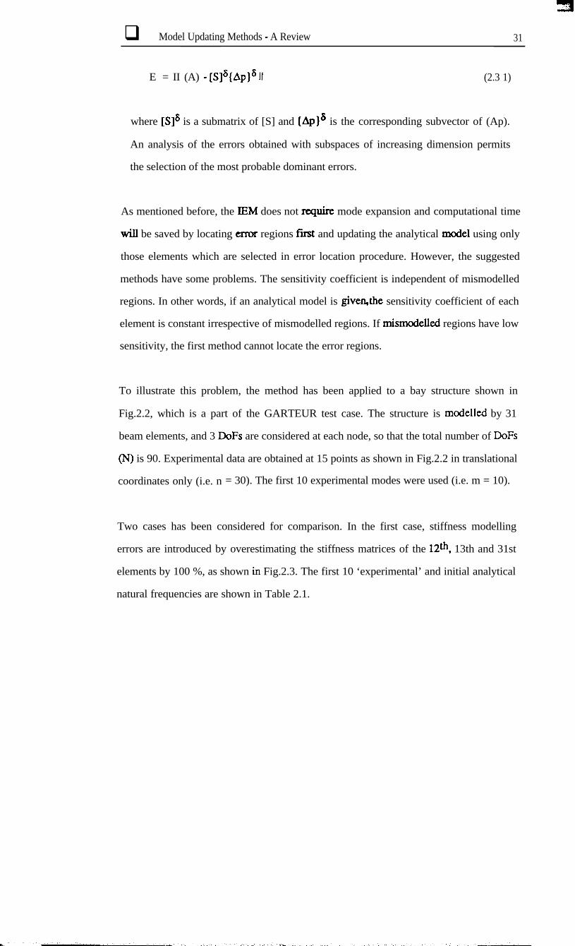
E = II (A) - [S]6(Ap]611 (2.3 1)
where [S]& is a submatrix of [S] and (Ap)” is the corresponding subvector of (Ap).
An analysis of the errors obtained with subspaces of increasing dimension permits
the selection of the most probable dominant errors.
As mentioned before, the IEM does not require mode expansion and computational time
wiIl be saved by locating error regions first and updating the analytical model using only
those elements which are selected in error location procedure. However, the suggested
methods have some problems. The sensitivity coefficient is independent of mismodelled
regions. In other words, if an analytical model is given&e sensitivity coefficient of each
element is constant irrespective of mismodelled regions. If mismcxlelled regions have low
sensitivity, the first method cannot locate the error regions.
To illustrate this problem, the method has been applied to a bay structure shown in
Fig.2.2, which is a part of the GARTEUR test case. The structure is modelled by 31
beam elements, and 3 DoFs are considered at each node, so that the total number of DoFs
(N) is 90. Experimental data are obtained at 15 points as shown in Fig.2.2 in translational
coordinates only (i.e. n = 30). The first 10 experimental modes were used (i.e. m = 10).
Two cases has been considered for comparison. In the first case, stiffness modelling
errors are introduced by overestimating the stiffness matrices of the 12th, 13th and 31st
elements by 100 %, as shown iu Fig.2.3. The first 10 ‘experimental’ and initial analytical
natural frequencies are shown in Table 2.1.

q Model Updating Methods - A Review 32
19 18 17 16 15 14 13
. Measurednodes
0 Unmeasured node:
Fig.2.2 Bay Structure
Table 2.1 Natural Fwencies of ‘Ex_perimentaI’ and Initial Analytical Models (Case u
The sensitivity coefficients and (Ap) are shown in Fig.2.4 and Fig.2.5 with possible
error regions. In this case, mismodelled regions which have relatively high
eigensensitivity could be located with some extra elements.

q Model Updating Methods - A Review 33
t
d (-1 -
d.--.-.-..-...-.--...-....-...-.2 4 6 8 10 12 Id 16 18 20 22 24 26 28 30
. (a)MassErrors
2 4 6 8 lo 12 14 16 18 20 22 24 26 28 30
Elm
(b) StiEness Errors
Fig.2.3 Modelling Errors

q Model Updating Methods - A Review 34
11
0.5
0.0
2
1
0
-1
-2
I2 4 6 610 12 14
r
16 16 20 22
(a) Eigensensitivity of Mass Element
lllllll24 26 26 30
Element
2 4 6 6 10 12 14 16 16 20 22 24 26 26 30
Element
(b) (=cxrection Coefficient
Fig.2.4 Error Location Results (Case 1 ; Mass Elemenmts)

q M&l Updating Methods - A Review 35
h6
1.8 10 14 16 18 20 :22 24 2f 28 30
E l m
(a) Eigensensitivity of Stiffness Elements
2
-2:...-. = -. .' .'.'. - - - ..'.'.'. -r-'2 4 6 8 10 12 14 16 18 20 22 24 26 28 30
Ekmen
Ib) Cofnxtion Coefficient
Fig.2.5 Error Location Results (Case1 ; Stiffness Elements)

q Model Updating Methods _ A Review 36
In the second case, mass and stiffness modelling errors are introduced by overestimating
the mass matrices of the 1 lth and 12th elements by 50 95 and the stiffness matrices of the
25th. 26th and 27th elements by 100 %, as shown in Fig.2.6. The fust 10 ‘experimental’
and initial analytical natural frequencies are shown in Table 2.2.
.mle 2.2 Natural Fregyencies of ‘J?x_~ntal’ and In’tial Analytul Models Case!1 21
i
The sensitivity coefficients and (Ap) are shown in Fig.2.7 and Fig.2.8 with possible
error regions. In this case, error location failed because some mismodelled elements have
relatively low eigensensitivity.
L..

q Model Updating Methods - A Review 37
(a) Mass Emrs
2-
l-
O- I I
-1 -
-2w - - - - - - _ - - - - - - - - - - - - - - ------.__2 4 6 6 10 12 14 16 16 20 22 24 26 26 30
Ekmalt
2
l-
0
-1 -
-2...............................2 4 6 8 10 12 14 16 16 20 22 24 26 28 30
Ekxnalt
(b)Stiffxless Errors
Fig.2.6 Modelling Errors (Case 2)

q Model Updating Methd - A Review 38
1.5 ,
1.0
0.5
0.0/
-2
1
0-y I
I
I
I 1,1,_
I I
4!_I____._________._____.~ I__y____
2 4 6 810 12 14 16 18 20 22 24 26 28 30
Elemmt
2 4 6 8 10 12 14 16 18 20 22 24 26 28 30
Ekmau
(a) Eigensensitivity of Mass Elements
4-
I SelectrdEkmcnts
2-
cb) Correction Coefficient
Fig.2.7 Error Location Results (Case2 ; Mass Elements)

q Model Updating Methods - A-Review 39
ll2 4 6 14 16
II2 4 26 28 30
Elanmt
(a) Eigensensitivity of Stiffness Elements
4
J
2 -
0 p,,,,,111
I
-2- I
0 Selected Elements
-4:. ..‘. nlml=s’* .== *. . . =***‘...=.2 4 6 8 10 12 14 16 18 20 22 24 26 28 3 0
Ekment
(b) Correction Coefficient
Fig.2.8 Error Location Results (Case2 ; Stiffness Elements)
The second method has been applied to the same structure. In both cases error location
failed as shown in Tables 2.3 and 2.4 - in the first case the 13th stiffness element was
not located and in the second case the 27th stiffness element was not located.
i ,, , ,. ,, ,.._ _,, -4% ,_,,. .:...

q Model Updating Methods - A Review 40
sI
1-2-3-4-56
-7
i-
-9
-10
-
L=lEmin
(& actual mismodelled element s; K12, K13, K31)
_‘.

02 Model Updaring Methods - A Review 41
.Table 2.4 Error Locwlts Case 21
s-1-2
2_4
I6
-7
F
9
-10
-
f
Located Elements
K25K25 K26K25 K26 Ml1K25 K26 Ml1 K28K25 K26 Ml1 K28 K9K25 K26 Ml1 K28 K9K30K25 K26 Ml1 K28 K9K30 Ml2K25 K26 Ml1 K28 K9K30 Ml2 K12K25 K26 Ml1 K28 K9K30 Ml2 K12 Ml6K25 K26 Ml1 K28 K9K30 Ml2 K12 Ml6 K31
IADI
0.67 0.69 0.220.63 0.64 0.42 0.190.26 1.05 0.40 0.46 0.180.34 0.94 0.24 0.38 -0.160.180.27 1.02 0.26 0.41 -0.130.38 0.110.30 0.97 0.21 0.39 -0.150.36 0.14 0.110.32 0.95 0.13 0.37 -0.090.35 0.28 -0.08 0.100.30 0.95 0.11 0.38 -0.100.35 0.27 -0.08 0.07 0.10
0.5670.592
0.6270.638
Emin
0.455
0.659
0.638
0.662
0.663
(cJ actual mismodelled elements; Ml 1, M12, K25, K26, K27)

q Model Updating Methods - A Review 42
2.4 CONCLUDING REMARKS
An attempt has been made to review various updating methods which can be divided into
two groups - direct methods and iterative methods. Direct methods are usually very fast
and some methods produce exact modal parameters, but mode expansion is essential
because of the large difference in the dimension between measured modes and the
analytical model. The problem of mode expansion is that this procedure might be
erroneous, thus jeopardising model updating procedure. On the other hand, iteration
methods such as IEM do not require mode expansion procedure and the updated model
can preserve physical co~ectivity and may become physically meaningful model - if it
converges. However, this method requires large computational effort because of repeated
solution of the eigendynamic problem and repeated calculation of the sensitivity matrix.
Also, convergence is not guaranteed if modelling errors are not small.
Any attempt to update every element in the analytical model using only the limited
information from typical test results may not be realistic. If mismodelled regions can be
located in a preliminq step, model updating can be carried out more efficiently and more
successfully. Therefore, error location is a fundamental fmt objective of the updating
process.
Recent developments in the area of error location have been investigated. The EMM can
locate mismodelled regions successfully even with a very limited number of measured
modes if complete coordinates are measured, which is not practical assumption. Again,
for the EMM to be successful, a reliable mode expansion method should be available.
The IEM does not require mode expansion and its computational time will be reduced by
locating error regions fmt and updating the analytical model using only the elements
which are selected in error location procedure. However, the methods suggested by

q Model Updating Methods - A Review 43
Zhang have been found to be unreliable. Themfore, more reliable error location method
should be developed.
? . . _ . , -

L

q Model Updating Using IEM 45
CHAPTER 3
MODEL UPDATING USING IEM
3.1 PRELIMINARIES
In the last Chapter, advantages and disadvantages (or limitations) of various model
updating methods were discussed and it was noted that all direct methods needed mode
expansion - and if this were erroneous, this might jeopardise the model updating
procedure - to overcome the incompatibility in the dimensions of the measured modes (n)
and the analytical model (N).
The IEM, which is one of iterative methods, has an advantage over direct updating
methods in the respect that it does not require a mode expansion procedure. However,
convergence is not guaranteed if modelling errors are not small. The convergence might
be improved by locating error regions fmt and by correcting only the selected parameters
by an iterative calculation. The methods suggested by Zhang [ 191 which are based on the
IEM do not seem to be reliable as shown in the case studies in the previous Chapter.
In this Chapter, a version of the IEM using arbitrarily chosen macro elements, which is
one of the iterative methods, is proposed at the error location stage in order to reduce the
computational time and to reduce the number of experimental modes required. By this

q Model Updating Using lEM 46
approach, the model updating problem which is generally under-determined can be
transformed into an over-determined one.
3.2 ERROR LOCATION PROCEDURE
3.2.1 SELECTION OF SUBMATRICES
The updated mass and stiffness matrices can be expressed as functions of the analytical
ones, in the form:
&I =k ai Wli (3.1)
(3.2)
where L is the number of elements and ai and bi are correction coefficients to be
determined. If there is no error in the ith element, ai and b, should be unity, whereas a; or
bi << 1 (or >> 1) indicates a mismodelled element. [M]i and [KJi are submatrices of
system matrices and can be one of these forms:
1) subelement matrices
2) element matrices used for FE modelling
3) macro element matrices
The success of the lEM depends heavily on the choice of the submatrices [MJ, and [Kli.
If the structure under consideration is a complicated structure - most practical structures
are usually very complicate& , it might have many elements and data from experiment are
usually very limited in the respect of the number of measured modes and the number of
measured coordinates. In such a case, model updating using the lEM with element

q Model Updating Using IEM 47
matrices or subelement matrices requires quite a large computational effort and the result
usually does not converge. The alternative is to use macro elements as submatrices.
The mass matrix of the im macro element Fl]i is formed as a summation of individual
element mass matrices
q
Flli zJz [M"lj (3.3)
where ni is the number of mass elements in the i* macro element and FI”lj is the element
mass matrix of the Jath element. The construction of the macro element is illustrated in
/ Appendix B.
Similarly, for the stiffness matrix
(3.4)
The influence of choice of macro elements on error location will be investigated later in
this Chapter.
3.3.2 EIGENSENSITIVITY
If we denote (p) as the vector of correction coefficients (a, % - at_ b, b, --- bJT, then
in the neighbourhood of (p,) = ( 1 l--l 1 l-1 IT, the rth eigenvalue of the updated
model can be expanded in a Taylor series:
(3.5)

q Model Updating Using EM 48
By neglecting the second- and higher-o&r terms, equation (3.5) can be approximated as:
(3.6)
Similarly, for the r* eigenvector
Inmatrixform
ax., 1I Ad
or
(4) (n+l) x 1 = [V (n+l) x 2L h-d 2L x 1
Aal...(1kAbl
Ai+_
(3.7)
(3.8)
(3.9)
The elements of the sensitivity matrix [S,] can be obtained by taking derivatives of the
following equations
with respect to the correction coeffkients as: [see Appendix A]
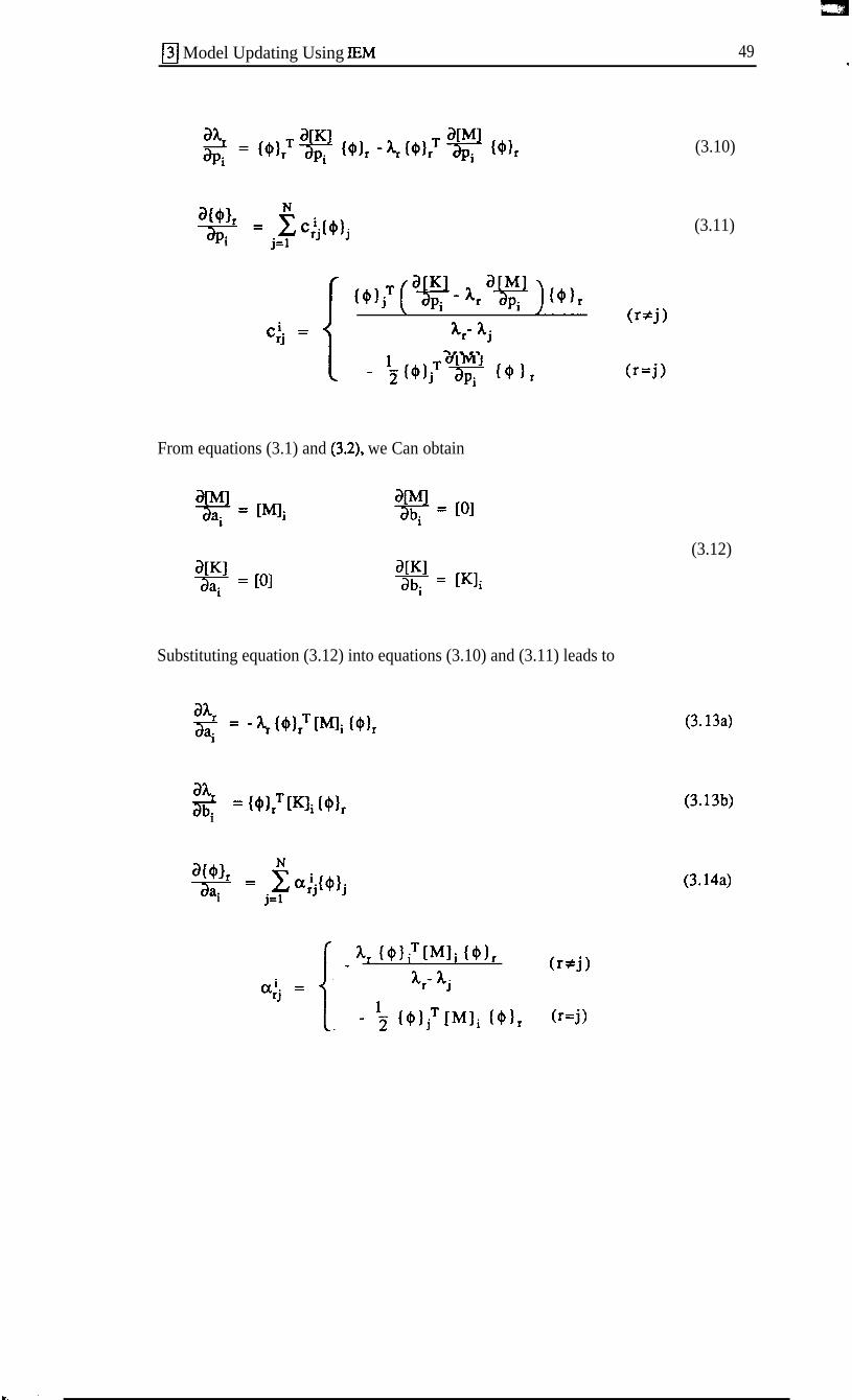
R Model Updating Using IEM 49
!$f$ = i c;j($)ji j=l
{
t4$ya~-~r~g-ycml,ci. =
*JX,- 3Lj
(NJ
aMI- ;NdjTJg- w, (r=j>
From equations (3.1) and (3.2), we Can obtain
arKi- = [O]aaiarK]- = [K]iabi
Substituting equation (3.12) into equations (3.10) and (3.11) leads to
3 = t@),TlKli ($1,i
!* = 5 a;j(+)ji j=l
1.- kr (@IiT [Mli IQ), (r#.i)aij = or- ~j
- f I@)jT [Mli (01, <r=j>
(3.10)
(3.11)
(3.12)
(3. Ida)
(3.13b)
(3.14a)

q Model Updating Using IEM
wo* = ,$ Pjj{@lj
(Q)iT EKli (+I,pi. =
rJ
~~- Xj
0
(r+j)
( r = j )
50
(3.14b)
Equation (3.14) requires N eigenvectors for the calculation of the eigenvector derivatives.
For a large system, only the lowest nl modes (q * N) can be expected to be computed
accurately. In addition, it may take long time to obtain N eigenvectors at each iteration
Lim et. al. [26] proposed a new method which could reduce the number of eigenvectors
I required for the calculation of the eigenvector derivatives. When r << nl, the denominator
of C~j in equation (3.11) can be approximated as:
h, - 5 = 31c- 3cj for j > n1
where XC is a value between 0 and the first non-zero eigenvalue.
(3.15)
where
From the orthogonality conditions
q Model Updating Using IEM 51
we get
Ior
[@I-‘[K - XC M]-1[4’]-T = ( [A] - XC [IJ )-’
Thus,
I [K - 3L, Ml-’ = [@I ( WI - al I-’ PIT
= N (@Ii (@Iicj=l 31j- h,
(3.16)
Substituting equation (3.16) into equation (3.15)
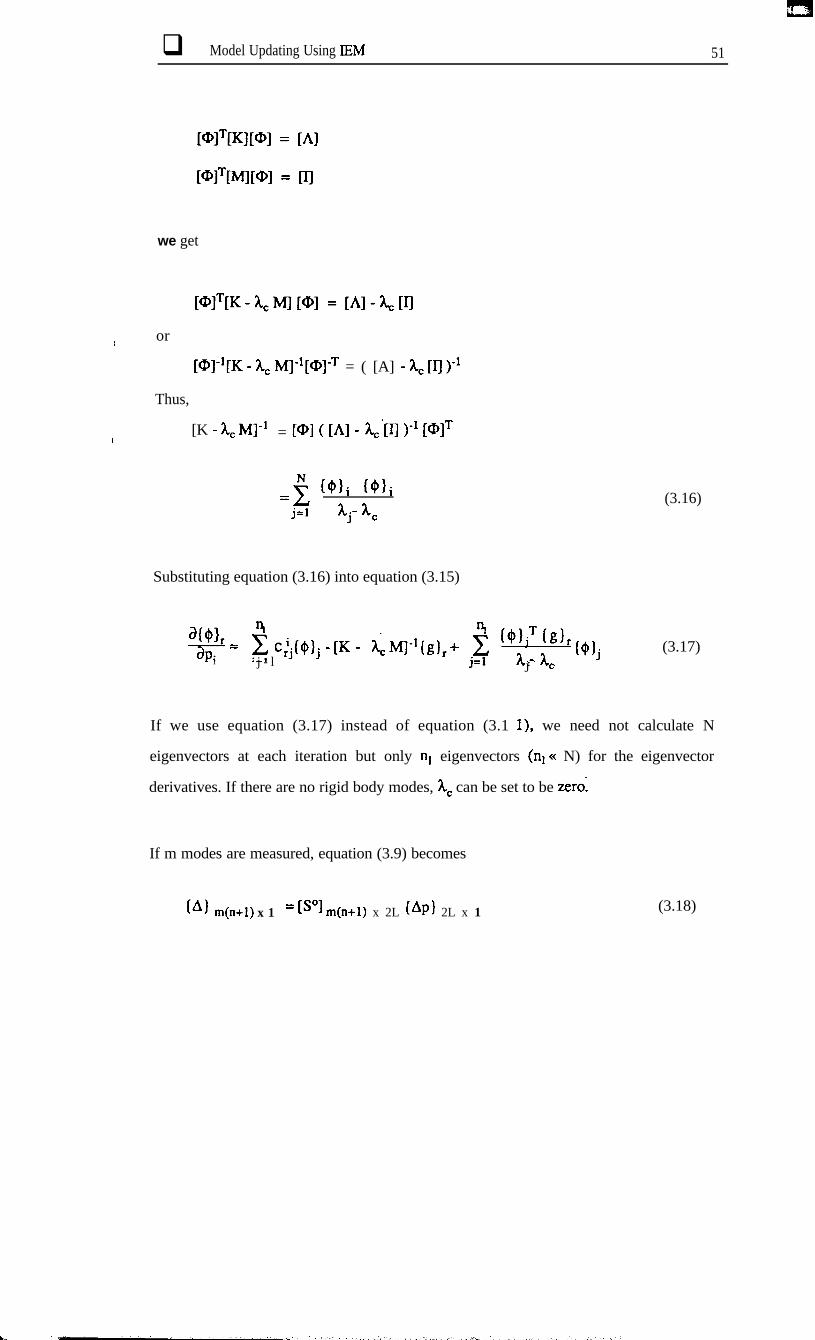
y = 2 c;j(Q)j - [K - c M]-l(g),+ 2 “;T:,)r (t$)j (3.17)i j - l j=l .-
J C
If we use equation (3.17) instead of equation (3.1 l), we need not calculate N
eigenvectors at each iteration but only n1 eigenvectors (n, << N) for the eigenvector
derivatives. If there are no rigid body modes, hC can be set to be zero:
! If m modes are measured, equation (3.9) becomes
(A) m(n+l) x 1 = [sol m(n+l) x 2L IAP1 2L x 1 (3.18)

.
q Model Updating Using lEM 52
3.2.3 COMPATIBILITY BETWEEN MEASURED MODES AND
ANALYTICAL MODEL
As mentioned in Chapter 2, modal parameters obtained from a modal test are generally
not compatible with those from the analytical model because
1) the number of modes available from measurement (m) is usually very limited
(m<cN) and
2) the number of measured coordinates (n) is in general much less than the number of
coordinates (or the number of degrees of freedom) of an analytical model (n&J).
The mismatch in the number of measured modes (m) and analytical modes (N) can easily
be overcome by using corresponding modes from the analytical model and omitting the
unmeasured modes. In the formulation of the lEM, a mode-to-mode matching between
the measured and analytical modes is essential. This matching can be performed by the
use of MAC (Mode Assurance Criterion) [27] which is defined by
(3.19)
It can be seen in the equation that the MAC values vary between zero and unity. If the
experimental and analytical mode shapes used for the MAC are from the same mode, a
value close to unity is expected, whereas if they relate to two different modes, a value
close to zero should be obtained. Given a set of mx experimental modes and a set of rn*
analytical modes, we can calculate the mx x mA MAC matrix, and use it to indicate which
test mode relates to which analytical one. The analytical modes which correspond to the
experimental modes are often not in the same sequence. The MAC matrix can sort out this
reordering. This procedure should be performed at each iteration.
: I,, . -. ̂ I -_* .._,.,l.. __,.‘.... _. , ,_ .:..:_., -.- I

q Model Updating Using IEM 53
The coordinate mismatch can also be overcome by using corresponding coordinates from
the analytical model and omitting the unmeasured coordinates in formulating equation
(3.7).
3.2.4 BALANCING THE SENSITIVITY MATRIX
One problem in equation (3.18) is that the sensitivity matrix may be ill-conditioned
because the magnitudes of the eigenvector derivatives are usually very small compared
with the magnitudes of the eigenvalue derivatives. From equations (3.10) and (3.11)
Therefore,
So, instead of equation (3.18), we can write
(3.20)
(3.21)
(3.22)

q Model Updating Using IEM 54
or
. . . . .
. . . . . .
IA) m(n+l) x 1 = PI m(n+l) x 2L IAP)2L x 1
Aa...
A al..Abl
.
.
4b,
(3.23)
A necessary condition for equation (3.23) to be over-determined is:
m(n+l)>2L or rn>-$I
However, the eigenvector sensitivities are not always linearly independent. In practice,
the number of measured modes should be more than twice of the minimum number in
order to give a high probability of sufficient rank to matrix [S]. Using the SVD technique
[49], the condition of the sensitivity matrix can be checked_ The technique also can be used
to solve (Ap). If [S] is full rank, equation (3.23) can be rewritten as:
{Al m(n+l) x 1 =Wl m(n+l) x m(n+l) [‘I m(n+l) x2L [‘lT2L x 2L IAP 1 2L x 1
(3.24)
where &Jl and [VI are orthonormal matrices and ]Z] is a matrix with elements Oij = CTi
(singular values of [S]) for i = j and Oij = 0 for i + j.

E Model Updating Using IEM 55
Because lu] and [VJ are orthonormal and full rank matrices, the solution of equation
(3.24) can be written as:
WP] = WI [El+ WIT IA] (3.25)
where + is the Moore-Penrose genera&d inverse and [Z]+ consists of the inverse values
of the non-zero Singular values ai.
The corrections are then added to the solution vector
(P] new = (~]cld + (ApI (3.26)
and the process is iterated to convergence because equation (3.25) is not the correct
answer since:
i) equations (3.6) and (3.7) are only fust-order approximations of eigenvalues and
eigenvectors, respectively, and
ii) subdomains do not necessarily auzord exactly with mismodelled regions.
The flowchart of the whole procedure can be seen in Fig.3.1.

q Model Updating Using IEM 56
Solve eigendynamic equalian to getr-- AAI’ W44
1calculate sensitivity matrix
b [S] and (A)
I
Solve the equation
Update solution vector
(PI,,= (P),,td+ bP)
I Calculate new mass and stiffness matrices I
I Solve eigendynamic equation to getnew modal parameters I
N
( S T O P )
Fig.3.1 Flowchart of Error Locating Procedure

q Model Updating Using IEM 57
3.2 NUMERICAL EXAMPLES
The bay structure which had been used in Chapter 2 was used again to check the validity
of the method suggested above. Mass and stiffness modelling errors were introduced by
overestimating the mass matrices of the 25th and 26th elements by SO 96 and the stiffness
matrices of the 12th. 13th and 31st elements by 100 96, as shown in Fig.3.2.
‘Experimental’ data were obtained for 15 points in translational coordinates only and the
first 10 ‘experimental’ modes were used, exactly as for the case studies in Chapter 2. The
first 10 ‘experimental’ and initial analytical models are shown in Table 3.1.
Table 3.1 Natural Frequencies of ‘Exoerimental’ and Initial Analvtical Models

q Model Updating Using IEM 58
2
1
0
-1
-2
2
1
0
-1
-2
2 4 6 6 10 12 14 lt 16 20 22 24 26 28 30
EknwxNumkrs
(a) Mass Errors
2 4 6 8 10 12 14 16 18 20 22 24 26 28 30Element Numbers
(b) Stiffness Errors
Fig.3.2 Modelling Errors
. ..,

q Model Updating Using IEM
3.3.1 INFLUENCE OF CHOICE OF MACRO ELEMENTS
ON ERROR LOCATION
59
In order to investigate the influence of the choice of macro elements on ezTor location, 4
different macro element configurations - Macro 1, Macro 2, Macro 3 and Macro 4
(Fig.3.3) - were used. In each case, no macro element coincided exactly with one of the
error regions.
6(5)
6(3:
Macro3 Macro4
4(5)
e(4)
hIacro2
* Macro Element No.(No.of Elements)
Fig.3.3 Macro Element Models

q Model Updating Using IEM 60
Using Macro 1, it took 4 iterations to converge and 20 elements - 9 mass elements and 11
stiffness elements - were identified as possibly harbouring modelling errors, as shown in
Figs.3.4(a) and 3.5(a). Similar results were obtained using other macro models as shown
in Figs.3.4 and 3.5. In each case, all mismodelled regions could be located in that they
were included in the sites found by the method.
0.5
0.0
-0.5
i
fb......rm..........fi.......I5 10 15 20 25 3 0
Element Numbers
(a) Macro 1
-0.5 ,,,,,,,....,.,.................5 10 15 20 25 30
-0.55 10 15 20 25 30
Element Numbers Element Numbers
(c) Macro 3 (d) Macro 4
0.5
0.0
-0.5
i
frl.....‘.................,..,,
5 10 15 20 25 30
Element Numbers
(b) Macro 2
( * ; Selected Elements )
Fig.3.4 Error Location Results (Mass Elements)

q Model Updating Using IEM 61
-0.5 ml....-...m.......w -0.5 r....m.mp5 10 15 20 25 30 5 10 15 20 25 30
ElanauNumbcrs Elanent Numbers
(a) Macro 1 (b)Macro2
0.5 0.5
. . . .. . . . . . .. . . .
0.0 0.0 --a”’
-0.5 -O.5rr.......~....-..,,,,.*5 10 15 20 25 30 5 10 15 20 25 30
Element Numbers Element Numbers
(c) Macro 3 (d) Macro 4
( * ; Selected Elements )
Fig.35 Error Location Results (Stiffness Elements)
As a second case study, the same errors as the second case in Chapter 2 were used, for
which case the two methods suggested by Zhang had failed to locate the error regions.
Error location was carried out using Macro 1 model. The results are shown in Fig.3.6,
from which it can be seen that the mismodelled elements (Ml 1, Ml 2, K25, K26 and
K27) were all located.

q Model Updating Using IEM 62
1
0
-1
q ; SeIected Elements
2 4 6 8 10 12 14 16 18 20 22 24 26 28 30
Element Nun&
(a) Mass Errors
q ; SelectedElements
2 4 6 8 10 12 14 16 18 20 22 24 26 28 30ElementNumfm
(b) Stiffness Errors
Fig.3.6 Error Location Results (Case 2)
. -.._ .Ibl . ..__I ___-
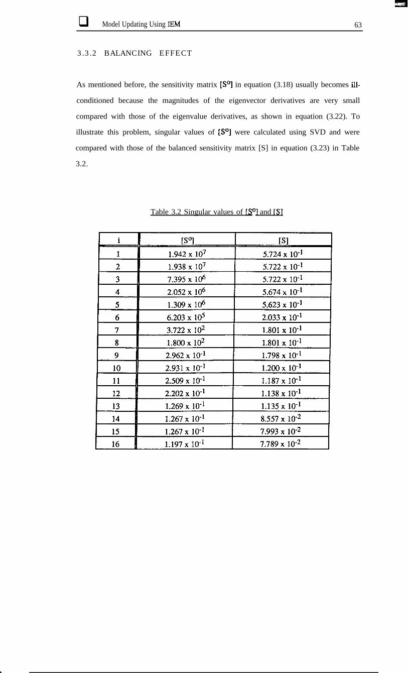
q Model Updating Using IEM 63
3.3.2 BALANCING EFFECT
As mentioned before, the sensitivity matrix [SO] in equation (3.18) usually becomes ill-
conditioned because the magnitudes of the eigenvector derivatives are very small
compared with those of the eigenvalue derivatives, as shown in equation (3.22). To
illustrate this problem, singular values of [SO] were calculated using SVD and were
compared with those of the balanced sensitivity matrix [S] in equation (3.23) in Table
3.2.
Table 3.2 Singular values of rS”J and fS]

q Model Updating Using IEM 64
The condition number - which is defined as the ratio of the largest of the aj’S to the
smallest of Oj’s - of [SO] is 1.63 x 10⁸, which is the indication of an ill-conditioned
matrix, whereas the condition number of [S] is 7.34.
The rank of [SO] can be calculated using SVD. If the rank of a matrix is r, then or+, will
be very small compared with the other singular values bi (i = 1,2;**,r). If we establish a
criterion for the rejection or acceptance of small singular values, we shall have an answer
concerning the value of the rank. This criterion may depend on the accuracy of the
expected results and, in practice, may be difficult to establish. A reasonable solution is to01 02calculate the consecutive ratios of the singular values - , - *.a, then the ratio or- will02 03 or+1
be very high compared with F. Therefore, the first peak or- will indicate the value ofor+1
the rank. The consecutive ratios of the singular values of [SO] are compared with those of
[S] in Fig.3.7. It can be seen from the figure that [SO] is rank deficient (the rank is 6)
whereas [S] is rank full.
Values of Api calculated based on the equation (3.18) are compared with those calculated
based on the equation (3.23) in Table 3.3. It can be seen the former are meaningless
because [SO] is rank deficient.

q Model Updating Using IEM 65
20-
-20. w n . -1. ."V"..'1 2 3 4 5 6 7 8 9 1 0 1 1 1 2 1 3 1 4 1 5
2c
0
-20 i
I
1 2 3 4 5 6 7 8 9 101112131415
(b) PI
I Fig.3.7 Rank of Sensitivity Matrix

q Model Updating Using IEM 66
Table 3.3 Comnarison of Correction Coefficients (1 st Iteration Results)
Mass
3.4 MODEL UPDATING PROCEDURE
After locating regions where modelling errors might exist, the model improved by the
error location procedure is refined by a modeI updating procedure. In the model updating
process, the variables to be updated are not the correction coefficients of the macro
elements but the correction coefficients of the individual elements from which the macro
elements are assembled for the preceding error location procedure. The problem to be
solved here is
@)m(n+l) x 1 = IS’1 m(n+l) x 1 (*P’)f x 1 (3.27)
where I is the number of the selected elements from the error location procedure.
Equation (3.27) is similar to equation (3.23). The differences are that Ap’represents the
correction coefficients of the element matrix which might have modelling errors and [S’]

q Model Updating Using IEM 67
represents the sensitivity matrix of the elements selected in the error location procedure.
Equation (3.27) should be solved iteratively because it is an approximate solution.
The IEM is, in fact, a multi-variable Newton-Raphson method. In Fig.3.8, the model
updating process using IEM is illustrated graphically for the case of one variable. The
slope of the curve L = f(p) at the point A@“,kAi) corresponds to the eigenvalue
sensitivity, and a segment AC corresponds to the solution of the equation (3.9). The
process BD is equivalent to the calculation of the eigenvalue problem w] ($) = kM { $}.
When modelling errors are not small, in which case the higher-order terms in the Taylor
series of eigenvalues and eigenvectors are important, the IEM can give grossly inaccurate,
meaningless corrections as illustrated in Fig.3.9.
AP’< >
>P”(= 1) P’ P
Fig.3.8 Pictorial Expression of the IEM
‘-

q Model Updating Using IEM 68
Fig.3.9 Unfortunate Case where the IEM Diverges
The convergence of the lEM can be improved by the following:
1) new initial guess and/or
2) setting bounds on (Ap’).
The resultant correction coefficients from the error location procedure can be considered
as “improved” new initial guesses and these usually improve the convergence because the
distance between the analytical and experimental models has been reduced by the error
location procedure. This statement is illustrated in Fig.3.10. The second strategy to
improve the convergence of the lEM is illustrated in Fig.3.11.
The flowchart of the whole procedure of the model updating can be seen in Fig.3.12.

q Model Updating Using IEM 69
0 ; Initial vahles
n ; Improved Values
>P
Fig.3.10 Model Updating with Improved Initial Guess
>
PO P
0;OriginalValuem;ModifiedValues
Fig.3.11 Model Updating by Setting Bound on Ap

q Model Updating Using IEM 70
Read the Output of Error hating Procedure .
Solve eigendynamic equation to get
Lb (Q,
Calculate sensitivity matrix(S’l and (A} 4
Solve the equation(43 = P’l+ (4
Update solution vector1 P’)lew= I P&j + b P’:
Calculate new mass andstiffness matrices
Solve eigendynamic equation to getnew modal parameters
N
Fig.3.12 Flowchart of Model Updating Procedure

q Model Updating Using IEM 71
3.5 APPLICATION TO BAY STRUCTURE
Using the error location result from the Macro 1 model of 6 3.3.1, updating has been
carried out. There were 20 elements identified which might contain modelling errors - 9
mass elements and 11 stiffness elements - as shown in Figs.3.4(a) and 3.5(a). The
iteration results are shown in Figs.3.13 and 3.14, from which it can be seen that the final
estimates become very accurate after 5 iterations.
Natural frequencies of the updated model are compared with experimental natural
frequencies together with MAC values in Table 3.4.
Table 3.4 Natural Freuuencies of ‘Exnerimental’ and Undated Models

cl3 Model Updating Using IEM 72
1
0 II I I II
-1 . - * - - - - - - - - = - - - - - ’ - - - - - - ’ ’ - - - - -
2 4 6 6 10 12 14 1 6 16 2 0 2 2 2 4 2 6 2 6 3 0Element Number!
(a) First Iteration
1
1 . . . . . . 1 l . - - ’ ’ ’ . = ’ 1 - - = . ’ ’ ’ ’ ’ ’ - - ’2 4 6 6 1 0 12. 1 4 1 6 1 8 2 0 2 2 2 4 2 6 2 8 3 0
Element Numbers(b) Third Iteration
1
I - - - - - - - -- - - - - - - - - - -2 4 6 8 1 0 1 2 1 4 1 6 1 8 2 0 2 2 2 4 2 6 2 8 3 0
Element Numbers(c) Fifth Iteration
Fig.3.13 Model Updating Results (Mass; Casel)

q Model Updating Using IEM 73
0 . II1
-2!.............................2 4 6 6 10 12 14 16 18 20 22 24 26 28 31
(a) First IterationElement Num
0 .I
a!.............................2 4 6 6 10 12 14 16 18 20 22 24 26 28 3C
(b) Third IterationElement Numl
0
a ! . . . . . . . - . - -2 4 6 8 10 12 14 16 18 20 22 24 26 28 30
(c) Fifth IterationElement Numb
Fig.3.14 Model Updating Results (Stiffness ; Casel)
*.

q Model Updating Using IEM 74
3.6 APPLICATION TO THE GARTEUR STRUCTURE
3.6.1 THE GARTEUR STRUCTURE
To check the validity of the aforementioned method to a practical structure, the method
has been applied to a free-free structure known as the GARTEUR structure (Fig.3.15).
The structure is modelled by 83 beam elements. It has 78 nodes and 3 DoFs are
considered at each node, so that the number of total DoFs of the analytical model is 234.
Each element is constructed by a superposition of an axial bar element and a bending
beam element, and these pairs of elements are considered to be independent of each other.
The element mass and stiffness matrices and necessary data are given in Appendix B.
r 7 8 9 10 11 12 13 14 15 16 17 18 19 20 2122 23 24 25 266
5
4
3
2
1
0 measured nodes0 unmeasured nodes
Fig.3.15 Free-Free GARTEUR Structure
Modelling errors are introduced in exactly the same way as those of GARTEUR 1
exercise - by overestimating the cross-section area of the 12*, 13*, 41st, 42”d, 59th and
60* elements by 100 %, and by underestimating the second moment of area of the 3 lst,
32d, 41s’ and 42d elements by 50 %. The exact modelling errors are shown in Fig.3.16.
h .,.

q Model Updating Using IEM 75
Fig.3.16 (a) Exact Modelling Errors (Axial Elements)

B Model Updating Using IEM 76
Fig.3.16 (b) Exact Modelling Errors (Bending Elements)

m Model Updating Using IBM 77
36 nodes are assumed to be ‘measured in two translational directions (u and v directions)
only as shown in Fig.3.15. The first 5 modes are assumed to be measured, and these and
the corresponding analytical natural frequencies are shown in Table 3.5 together with
their MAC values.
Table 3.5 Natural Freouencies of ‘Exoerimental and initial Analvtical Models
3.6.2 EIGENSENSITIVITY
In this exercise, it is not appropriate to express the updated stiffness matrix in the form of
equation (3.2) and more independent physical design variables need to be considered.
Because the cross-section area and area moment of inertia are considered to be
independent variables, the updated stiffness matrix can be expressed as:
L
IX"1 =,z Cj P&lj + Ik dj IKbIjj=l
where [Kalj is the axial element stiffness matrix which is proportional to the cross-section
area and [Kblj is the bending element stiffness matrix which is proportional to the second
moment of area.
The eigensensitivities can be easily derived as:

q Model Updating Using IEM 78
y = i y;j($)ji j=l
(+I: lIK,li (01,r;lj = Xr- Xj
0
~$pr = g s;j($)ji j=l
6’. =rJ
(wi 1
(r=j>
(wj>
(r=_i>
3.6.3 ERROR LOCATION PROCEDURE
In the error location procedure, 26 macro elements were used as shown in Fig.3.17. No
macro element coincides exactly with the error regions.
1 h(4) 1X3) 14(4) 13(3) 12~4) 1 X3)
* ; Macro Element No.(No. of Elements)
Fig.3.17 Macro Elements of GARTEUR Structure
c

q Model Updating Using lEM 79
The iteration results are shown in Fig.3.18 and Table 3.6. After 7 iterations, the analytical
model converged to the experimental model and it became possible to locate possible error
regions - 10 axial and 8 bending macro elements, or 32 axial and 34 bending elements.
Table 3.6 Natural Freuuencies of ‘Exnerimental’ and Intermediate Amd~tical Models
/ 3.6.4 MODEL UPDATING PROCEDURE
After locating possible error regions, the updating was carried out with the correction
coefficients calculated as initial values. It can be seen in Figs.3.19 and 3.20 that estimates
becomes very accurate after 8 iterations. The natural frequencies of the updated analytical
model are compared with those of the experimental model in Table 3.7 together with
MAC values.
Table 3.7 Natural Frequencies of ‘Fxnerimental’ and Updated Analvtical Models

q Model Updating UsinglEM : 80
Fig.3.18 (a) Error Location Results (Axial Elements ; After 7 Iterations)
‘s.

q Model Updating Using IEM 1 81
-
Fig.3.18 (b) Error Location Results (Bending Elements ; After 7 Iterations)

q Model Updating Using IEM 82
Fig.3.19 (a) Model Updating ResuIts (2nd Iteration ; Axial Elements)

q Model Updating Using IEM 83
Fig.3.19 (b) Model Updating Results (4th Iteration ; Axial Elements)

q Model Updating Using .IEM 84
Fig.3.19 (c) Model Updating Results (6th Iteration ; Axial Elements)
c

q Model Updating Using IEM 85
Fig.3.19 (d) Model Updating Results (8th Iteration ; Axial Elements)
. , .,. .

q Model Updating UsingJEM 86
Fig.320 (a) Model Updating Results (2nd Iteration ; Bending Elements)

q Model Updating Usipg IEM 87
Fig.3.20 (b) Model Updating Results (4th Iteration ; Bending Elements)

q Model Updating Using IEM 88
Fig.3.20 (c) Model Updating Results (6th Iteration ; Bending Elements)

r
q Model Updating Using IEM 89
Fig.3.20 (d) Model Updating Results (8th Iteration ; Bending Elements)

q Model Updating Using IEM 90
3.7 CONCLUDING REMARKS
One of the advantages of model updating using eigensensitivity analysis is that mode
expansion (or reduction) is not required. However, this method requires large
computational effort because of the repeated solution of the eigendynamic problem and
repeated calculation of the sensitivity matrix. In this Chapter, a sensitivity method using
arbitrarily chosen macro elements has been proposed at the error location stage to reduce
the computational time and to reduce the number of experimental modes required for
subsequent updating. By this approach, the model updating problem, which is generally
under-determined, can be transformed into an over-determined one and the updated
analytical model is not influenced by the definition of macro elements.
It has been illustrated that the IEM is a multi-variable Newton-Raphson method and the
convergence of the IEM can be improved by introducing error location procedure and by
setting bounds on { Ap).
The proposed method has been applied to the free-free GARTEUR structure which may
represent a practical structure and constitute a realistic problem in respect of the
incompleteness of both measured modes and coordinates. The updating results are quite
accurate not only in modal parameters but also in correction coefficients of physical
design variables.
The ‘experimental’ data of the case studies in this Chapter are noise-free data. However,
because of various measurement errors, the assumption that the test results represent the
’ true dynamic behaviour of the structure may not be correct - the experimental data can be
affected by several types of measurement error. Thus, the sensitivity of the updating
method itself to noise on the experimental data needs to be investigated.


q Error Sensitivity of the Inverse Eigensensitivity Method 92
1 CHAPTER 4
ERROR SENSITIVITY OF THE INVERSEEIGENSENSITIVITY METHOD
4.1 PRELIMINARIES
One of the most important objectives of modal testing is to validate the analytical model of
a dynamic structure by comparing experimentallydetermined modal parameters - which
are supposed to be correct - with those obtained from an analytical model. However,
because of various measurement errors, the assumption that the test results represent the
true modal parameters may not be correct.
To check the validity of a model updating method by numerical case studies,
measurement errors must be considered. Even though many methods have been
developed in recent years for updating analytical models for the dynamic analysis of a
structure, and some of them have been proven to be quite successful, the methods are
k generally based on the assumption that the test data are perfect or noise-free. For any
updating method to be useful for practical structures, the sensitivity of the method to
noise on the test data needs to be established.
L,

q Ermr Sensitivity of the Inverse Eigensensitivity Method 93
In this Chapter, typical measurement errors will be introduced by contaminating the
modal parameters of the correct or modified structure with random noise of different
noise levels to check the sensitivity of the IEM to noise on the test data.
4.2 SENSITIVITY OF IEM TO NOISE ON MODAL
PARAMETERS
The IEM described in Chapter 3 has been applied to the bay structure which had been
used in Chapter 2 and Chapter 3 to check the error sensitivity of the method. Mass and
stiffness modelling errors were introduced by overestimating the mass matrices of the
‘25th and 26th elements by 50 96 and the stiffness matrices of the 12*, 13th and 31St
elements by 100 % as shown in Fig.3.2. Experimental data were obtained at 15 points in
translational coordinates only and the first 10 “experimental” modes were used, as the
case studies in Chapter 2 and Chapter 3.
4.2.1 ERROR LOCATION PRoCEDURE
4.2.1.1 Sensitivity to Measurement Noise
In order to investigate the sensitivity of the error location procedure to noise on the
experimental data, the simulated experimental modal parameters were contaminated by 4
different random noise levels - NLl (no noise), NL2 (0.2% in eigenvalues and 2% in
tigenvectors), NL3 (0.5% in eigenvalues and 5% in eigenvectors) and NL4 (1% in
eigenvalues and 10% in eigenvectors).
.

q Error Sensitivity of the Inverse Eigensensitivity Method 94
The error location procedure was carried out using the Macro 1 model shown in Fig.3.3,
and the results are shown in Fig.4.1. In each case, all mismodelled regions can be
: located.
0.:
0.0
- 0 . 5
m NLl0 NL2lsB]I N L 3q NL4
2 4 6 6 10 12 14 16 18 20 22 24 26 28 30Ekmat Numbers
(a) Mass Modelling Errors ( * ; Selected enernents)
I NLlCl NL2
NL3fl NL4
-l.... . . . . . . . . . . . . . . . . . . . . . * . . . . .2 4 6 8 10 12 14 16 18 20 22 24 26 28 30
Element Numbers
(b) Stiffness Modelling Errors (*; Selected elements)
Fig.4.1 Error Location Results (Macro Model ; Macrol)
1

m Error Sensitivity of the Inverse Eigensensitivity Method 95
4.2.1.2 Influence of Choice of Macro Elements on Error Location
In order to investigate the influence of choice of macro elements on error location, 4
different macro element configurations - Macro 1, Macro 2, Macro 3 and Macro 4
(Fig.3.3) - were used for error location. In each case, no macro element coincided exactly
with the error regions. NL3 experimental data - 0.5% random noise in eigenvalues and
5% random noise in eigenvectors - were used. The error location results are shown in
Fig.4.2, and again, all mismodekl regions have been located in each case.
4.2.2 UPDATING PROCEDURE
Using the results from the Macro 1 model and the NL3 experimental data - 0.5% random
noise in eigenvalues and 5% random noise in eigenvectors - updating has been carried
out. Natural frequencies of the “experimental” and initial analytical models are shown in
Table 4.1 together with the mode shape correlations indicated by MAC values.
Table 4.1 Natural Freuuencies of “ExDerimental” and Initial Analvtical Models
20 elements were indicated as possibly having modelhng errors - 9 mass elements and 11
stiffness elements - as shown in Fig.4.1. All the eigenvalue sensitivities were used
because eigenvalues can be measured more accurately than eigenvectors. If the number of
measured modes (m) is greater than the number of unknowns (l’), only eigenvalue
L i’

B Error Sensitivity of the Inverse Eigensensitivity Method 96
0 . 5
I
Fi macro 1macro 2
!!!imacro 3macro 4
-0.5 ! . 1 . . . . . . . . . . . . . . . . . . . . . . . . . * . .2 4 6 8 1 0 1 2 1 4 1 6 1 8 2 0 2 2 2 4 2 6 2 8 3 0
Element Numbers
(a) Mass Modelling Errors
1
!macro 1macro 2macro 3
EI macro 4
-1 ! . . . . . . . . . . . . . * . . . . . . r . . . . . . . . .2 4 6 8 1 0 1 2 1 4 1 6 1 8 2 0 2 2 2 4 2 6 2 8 3 0
Element Numbers
(b) Stiffness Modelling Errors
Fig.4.2 Error Location Results (Noise Level; NL3)
b ,”

q Error Sensitivity of the Inverse Eigensensitivity Method 97
sensitivities need to be used for the calculation of the unknowns. If not, the eigenvector
sensitivities should be included in the sensitivity matrix so that the equation (3.27) is
overdetermined The minimum number of eigenvector sensitivity vectors to be used (m’)
can be calculated as
m + n m’> 1’
Thus,
m’ 2 1’ - mn
, In this particular case ( m = 10, n = 30,l’ = 20 ), the minimum number of eigenvector
sensitivity vectors needed is one. Between one and ten eigenvector sensitivity vectors
were used in the case study. When one or two eigenvector sensitivity vectors were used,
the updating results failed to converge. However, the updating results did converge, and
to the correct answers, as the number of eigenvector sensitivity vectors was increased.
The results are shown in Fig.4.3 and Fig.4.4. Natural frequencies of the updated model
using 10 eigenvector sensitivity vectors are given in Table 4.2. It can be seen that
estimation has become quite accurate for this case.
Table 4.2 Natural Freouencies of “Experimental” and &x&ted Analytical Models
k

q Error Sensitivity of the Inverse Eigensensitivity Method 98
.- Element 8---+--- Element 9--+---- Element 10- Element 11
. . . . .-1 . . . . . . . . . . . . . . . . . . . . . . . . . . . . . . .. .. . . Element12
I II -2 I’ I I I I I
2 4 6 8 1 0 1 2
No. of Modes
2I
1Element 25
--+-.-. Element260 ---a-- Element27
- Element28
-’ -2 ! I I I I I
2 4 6 8 1 0 1 2
No. of Modes
Fig.43 Model Updating Results - Mass Elements
(Macro 1, NL3)

q Ermr Sensitivity of the Inverse Eigensensitivity Method 99
2 ,-x..x,,‘..:.. I
“.. . .._xtt’ ::.... ,a. ..
_,, _. . . .._ z... _%.’ v. * \,
1 ‘. . . . . . . .%.I
,- Element 8---+--- Elunent9-#-- Element 10_
. _~r Element 11
-1 . . . . . . . . . %> . . Elanent 12
2 4 6 8 10 12No. of Modes
0
-1
-2 I I I I2 4 6 8 10 1 2
No. of Mocks
Elanent 13..L Element 14--. Elanent 15
Element29--.-+-- Element30---+--- Element 31
-1 - I
2 4 6 8 10 1 2No. of Modes
Fig.4.4 Model Updating Results - Stiffness Elements(Macro 1, NL3)
i- 1 . _i,.,‘.,..,., c ..L__ ..- ~ ,. .-,I

m Error Sensitivity of the Inverse Eigensensitivity Methd 100
4.3 CONCLUSIONS
Model updating using arbitrarily chosen macro elements has been applied to a bay1 structure for which “experimental” data are noisy and incomplete. The error location
procedure has been found to be very insensitive to the “measurement” errors - in the
presence of measurement errors of up to 1 96 in the eigenvalues and 10 % in the
eigenvectors, it succeeds in locating the mismodelled regions. The updating results are
quite accurate in terms of modal parameters and, moreover, in terms of correction factors,
when sufficient eigensensitivity terms are used. In this case study, measurement errors
were introduced by contaminating the modal parameters of the correct or modified
structure with random noise.
However, in practice, the characteristics of the measurement errors might not result in
random variations in the modal parameters. For the updating method to be useful in
practical application, various error sources in testing - such as the mass loading effect of
transducers, shaker/structure interaction, etc. - should be considered and more realistic
errors rather than random noise should be included in the “experimental” data.
.

i
I
t

5q Errors Involved in Modal Parameter Estimation from Test Data 102
CHAPTER 5
ERRORS INVOLVED IN MODAL PARAMETERESTIMATION FROM TEST DATA
5.1 PRELIMINARIES
In Chapter 4, measurement errors were introduced by contaminating the modal
parameters of the correct or modified structure with random noise of different levels to
check the sensitivity of the IEM to noise on the test data. In practice, however, realistic
measurement errors might not be represented by random errors on the modal parameters.
For the updating method to be practical, various error sources in testing should be
considered in detail and more realistic errors should be included in the “experimental”
data. Therefore, the errors involved in modal parameter estimation from the test data will
be discussed in detail, and the resultant “experimental” modal data which contain possible
experimental errors will be used to update the corresponding analytical model to check the
validity of the IEM.

.tl5 Errors Involved in Modal Parameter Estimation from Test Data 103
5.2 MODAL TESTING OF SAMM STRUCTURES
5.2.1 DESCRIPTION OF TEST STRUCTURESf
Vibration measurement was carried out with real structures called SAMM2A and 2B
structures which had been used for the project to assess the State-of-the-Art of Mobility
Measurements (SAh4M) [28] to illustrate some measurement errors. The structures can be
seen in the F&.5.1. Two substructures 2A and 2B could be bolted together at two points
by connecting adapters to form a complete structure 2C.
(a) SAMM2A
(b) SAMh42B
Fig.5.1 Test Structures

0 5 Errors Involved in Modal Parameter Estimation from Test Data 104
5.2.2 MEASUREMENT
In turn, each of the structures was suspended by light elastic bands to approximate a free-t
free condition. The highest rigid-body mode frequency was less than 10 % of that for the
lowest elastic mode of the structures.
The frequency range of interest was 0 - 2.4 kHz, and this range was divided into 3 equal
frequency ranges: 0 -
SAMM2B - which are
0.8 kHz, 0.8 - 1.6 kHz and 1.6 - 2.4 kHz. SAMM2A and
linear and lightly damped structures - were tested using three
different excitation signals: pure random, pseudo-random and impact. When the
excitation to the test structure is random or pseudo-random, it is necessary to use a push
rod to connect the exciter to the test structure. Ideally, the push rod should be infinitely
stiff for transmission of axial force, yet have zero bending stiffness to allow no moment
or lateral force transfer [29]. A practical compromise to this ideal is needed to prevent the
combination of the dynamics of the push rod - exciter system with those of the structure.
Two push rods with different lengths were used to check the validity of the data obtained.
The dimensions, properties and resonant frequencies of push rods can be seen in the
Appendix D.
FRFs obtained using different excitation techniques are presented in Fig.5.2 to Fig.5.7.
As can be seen in the plots, all the techniques gave similar results. Discrepancies between
various excitation techniques are found at the resonance frequencies of the test structures.
These discrepancies clearly indicate the leakage problem associated with light damping.
Because pseudo-random is essentially periodic, it does not suffer from leakage errors. On
’ the other hand, the nonperiodic techniques (pure random and impact) suffer from leakage
or window errors [29]. Another discrepancy - frequency shifts - can be found above 1.4
kHz (SAMM2A) and above 1.1 kHz (SAMM2B). These shifts result from the effects of
the connection of the exciter to the test structure. On the other hand, in the case of impact
testing there is no need for any connection, which means the resonance frequencies from

cl5 Errors Involved in Modal Parameter Estimation from Test Data 105
_r.___17_ ~ - .~. ._. -,- _.-_ _
0.00 F r e q u e n c y H z . 801 .QQ
SAMM2A HI 1
+60.00
- 6 0 . 0 3
0 . 0 0
S9MM2A HI2
I
--7---7----Y
F r e q u e n c y H r . 8 0 1 . 3 0
- 6 0 . 0 0 T - - - - - - - - J
0 . 0 0
SRMM2R H 2 2
F r e q u e n c y H z . 801.03
t
Figs.2 Comparison of FRFs from Different Excitation Techniques
(SAMM2A ; 0 - 800 Hz)

m Errors Involved in Modal Parameter Estimation from Test Data 106
t
+60.00-J I I
II
- 6 0 . 0 0- - - r - - - - - - -
_ - _ . _ -__-, _ _ _ _ _,
6 0 0 . 0 0 Frequent y Hz. 1 6 0 1 . 0 0
SAMM2A H I 1
_-- ~__ -+60.00 1
-60.001 , , ,
8 0 0 . 0 0 F r e q u e n c y H z .
SRMM2R H 1 2
+60.007 -------?1’
-se-OO~--T----i------i
000.00SAMM2A H 2 2
Frequent y Hz. 1601 .00
Fig.5.3 Comparison of FRFs from Different Excitation Techniques
(SAMM2A ; 800 - 1,600 Hz)

m Errors Involved in Modal Parameter Estimation from Test Data 107
1 1
-60.00 j, __‘_____‘__ ___-_j,
1600.00 F r e q u e n c y Hz, 2 4 0 1 . 0 0
SAMM2R Hl I
+60.00r---__-_____
!
1-6O.Q8 a/
+-,.--‘.r___,- .T- __- _.~ ._ -_,--_-(
1 6 0 0 . 0 0 F r e q u e n c y H z . 2401 ,013
SAMki2A H 12
+60.03]- ---.-_-. -_--.
i
w .7^$m-
r(’5x; 0E m:
.j
E?E v-w;1‘,
1
j-60.00_j_.____T _ _,_-_-__,-_-_-:____ 7 __. , , __ _. .-;
1 6 0 0 . 0 0 F r e q u e n c y H z . 2 4 0 1 . 0 0
SRMM2A H 2 2
Fig.5.4 Comparison of FRFs from Different Excitation Techniques
(SAMM2A ; 1,600 - 2,400 Hz)

I-YlErrors Involved in Medal Parameter Estimation From Test Data 108
t
-60.00 I _.__]
0.00 Frequent y Hz. 001.00
SAMM2B Hl 1
-_. - - - - - - - __-___-+60.33
I
- 6 0 . 0 0h
7-------T -I-di
6.00 Frequent y Hz. 80!.@3
S”MM2l3 -‘I2
+60 001 11
:: ‘Zz z\FE? 0.-iTim\” -53: _
i
!
’- 6 0 . 0 0 f__.__, ___I_____r __._ __. ___Ij
0 . 0 0 F r e q u e n cy H z . BBI.00
SflMM2B H 2 2
Fig.5.5 Comparison of FRFs from Different Excitation Techniques
(SAMM2B ; 0 - 800 Hz)
~ -,. , ,-lir, .._ ,_ ;, __,.‘.___ ,., ._ a-‘... ---

05 Errors Involved in Modal Parameter Estimation from Test Data 109
___~____. ___ -~__- -
I
I-60.00 I , l_.__ ..,. - __ _~. -.
-----“~- - -r--- ,--. 4:Frequency Hz. i50l .a0
+60.00---- -------
1 I
-60.0&__. _..I_T-
I_-_7---r-----I
800.00
SRMr-12 i3 3 i 2
F r e q u e n c y H z 1601.00
-60.00Y+_ - ,._. “-l - ---1-___..-,- .._ :... - , ._-- ___I
EOC.CC frequency Hz. !SQ! .02
S~VX2 a 222
Fig.5.6 Comparison of FRFs from Different Excitation Techniques
(SAMM2B ; 800 - 1,600 Hz)

05 Errors Involved in Modal Parameter Estimation from Test Data 110
_~~--.-+60.00
&JL+q
-60. OO~____,__T__-,___-_J
1600.00SAMM2B HI I
Frequency Hr. 2401 .00
+60.00-f--------.------
- - -------------lI
-60.00-jr. ._ _,1 _ :~____. ---,_.._., -. _,_
S3;r-!i,12 B V ! 2
___-_ ---._. .._. ._+66.0C
-60.00 ! , , ,~-----T---i
1600.00 Frequency Hz, 2401.00SAMIl2 B H22
Figs.7 Comparison of FRFs from Different Excitation Techniques
(SAMMZB ; 1,600 - 2,400 Hz)

cl5 l?rt’ors Involved in Modal Parameter Estimation from Test Data 111
impact testing are correct. The gain in quality using an exciter was not considered large
enough to justify the extra effort. In addition, the frequency shifts caused by the
dynamics of an exciter-push rod system were too considerable to be ignored in the
’ frequency range of interest.
5.3 ERRORS IN MODAL PARAMETER ESTIMATION
! The characteristics of the real errors in experimentally-measured modal parameters might
not be random, as supposed for the case in Chapter 4. For the updating method to be
practical, various error sources in testing should be considered and more realistic errors
1 should be included in the “experimental” data used for method validation.
The errors involved in modal parameter estimation can be categorised in three groups -
measurement errors, signal processing errors and analysis errors, all of which will be
discussed in detail in the following sections.
5.4 MEASUREMENT ERRORS
54.1 NONLINEARITY OF STRUCTURE
One of the fundamental assumptions of modal analysis is that the structure is linear. This
means that doubling the magnitude of the excitation force results in a doubling of the
4 response, and that if two or more excitation patterns are applied simultaneously, the
response of the structure is the sum of the individual responses to each of the forces
acting alone. For many important kinds of structure, however, this assumption is not
valid. There are many reasons for the system to be nonlinear:
1) violation of “small displacement” theory;

q Errors Involved in Modal Parameter Estimation from Test Data 112
i
2) rattling of loosely fastened components;
3) nonlinear stiffness; or
4) nonlinear damping
Nonlinearity in the structure may shift energy from one frequency to many new
frequencies thereby resulting in distortions in the measured FRF curves. One way to
reduce the effect of nonlinearity is to randomise these contributions by using random
excitation. Subsequent averaging will reduce these contributions in the same way as!
random noise is reduced.
5.4.2 NONSTATIONARITY OF STRUCTURE
Another fundamental assumption of modal analysis is that the structure’s properties are
stationary. This means that the modal parameters of the structure are constant with time.
Sometimes, the behaviour of a structure may change during the measurement period
because of slipping joints or loosening bolts, etc. This kind of measurement error should
be excluded on the test site by closely-controlled experimental procedure.
5.4.3 MASS LOADING EFFECT OF TRANSDUCERS
When an accelerometer is mounted on a structure, the increase in overall mass combined
with a change in the local stiffness will inevitably alter the dynamic properties of the
structure. The acceleration of the part of the structure near the accelerometer and thet
resonance frequencies of the structure are modified according to the following
relationship [30]:
+at*a
(5.1)

05 Errors Involved in Modal Parameter Estimation from Test Data 113
where h ; rrxxmrd accelerationat; true accelerationf, ; measured resonance frequencyft ; true resonance frequency
m ; effective mass of that part of the sttucture to which the accelerometer ismounted
ma; accelerometer mass
As a general rule, the accelerometer mass should be less than one tenth of the apparent
mass of the modes of the structure. When the added mass is of the same order as the
apparent mass of the modes of the structure, mass cancellation becomes essential.
54.4 ERRORS BY TRANSDUCER CHARACTERISTICS
5.4.4.1 Useful Frequency Range
The upper limit for measurements can be set to 30 % of the accelerometer’s own natural
frequency so that vibration components measured at this limit will be in error by less than
+ 10 % or to 20 % for errors of less than + 5 % if the accelerometer is properly fixed to
the test structure. It should be noted that an accelerometer’s useful frequency range is
significantly higher, i.e. to i or : of its resonance, where 3 dB linearity is acceptable.
5.4.4.2 Transverse Sensitivity
tThe transverse sensitivity of an accelerometer is its sensitivity to accelerations in a plane
perpendicular to the main transducer axis. The transverse resonance frequency is just
outside the upper frequency limit. At frequencies less than 16 % (10 %) of the main axis
resonance frequency, transverse sensitivity can be kept below 10 % (3 %). The

05 Errors Involved in Modal Parameter Estimation from Test Data 114
transverse sensitivity can be reduced by aligning the minimum transverse sensitivity axis
in the direction of maximum transverse acceleration.
5.4.4.3 Mounting Effect
The method of attaching the accelerometer to the measurement point is one of the most
critical factors in obtaining accurate results from measurements. Poor mounting results in
a reduction in the mounted resonance frequency, which can severely limit the useful
frequency range of the accelerometer. There are various methods of attaching the
accelerometer to the test structure - such as stud mounting, cementing stud mounting,/
wax mounting, magnet mounting, etc. The advantages/disadvantages of various methods
can be found in Refs.[29,30].
Local stiffness changes introduced by attaching the accelerometer to the structure should
also be considered when it is attached to a flexible surface [29].
5.4.5 SHAKER/STRUCTURE INTERACTION
When the excitation to the structure is a continuous signal, such as random or sinusoidal,
a shaker must be attached to the structure, usually incorporating a force transducer. So
long as the motion at the driving point of the shaker attachment remains colinear with the
shaker axis, the dynamics of the excitation system can be removed by mass cancellation
t techniques. However, if the motion at the driving point includes rotation or transverse
displacement, the resulting contamination of test data can no longer be removed. The
solution is to attach the shaker to the suucture through a push rod, which should have
high axial stiffness for transmission of axial force but low lateral or bending stiffness to

05 Errors Involved in Modal Parameter Estimation from Test Data 115
allow little moment transfer. Guidance on how to design the push rod can be found in
Refs.[3 1,321.
i Apart from the effect of the push rod, shaker/structure interaction causes ‘notches’ in the
input force spectrum at resonances of the structure [29,33]. Because little force is
required to produce a large response near resonances, a large amount of the force
generated in the shaker is used to excite the armature mass of the shaker. Fig.5.8 shows
shaker/structure model.
-
rRush Rod
X
ms -1
Shaker
Force Transducer
Fig.5.8 Shaker/Structure Interaction

cl5 Errors Involved in Modal Parameter Estimation from Test Data 116
The actual force applied to the structure can be calculated as follows:
p=f+m,Y
Fourier transform of equation (5.2) becomes
P(o) = F(o) + m, H(o) F(o)
Thus
F(U) = Hi(U) P(O)
(5.2)
(5.3)
where H(o) is an inertance and
Hi(U) = 11 + m, H(o)
If P(o) is constant, the power spectra of input force and output response can be
expressed as
GE(O) = I Hi(O) I 2 GPP
Gpp= ( l+msH(o))( l+msH*(o))
Gpp= 1 + ms* [ ( Re(H(o))12 + Um(H(W) I21 + 2 ms RG-W))
(5.4)
GAA(~) ==
1 H(o) 1 2 G&O)
I Hi(W) I 2 I H(U) 12Gpp (5.5)

05 Errors Involved in Modal Parametq Estimation from Test Data 117
5.4.6 MEASUREMENT NOISE
lf measured signals f(t) and a(t) are contaminated by measurement noise, m(t) and n(t)
respectively, as in F&.5.9, the FRF can be expressed as [34]
HI@) = GFA(@ WN
GFF((@ = l+ri
H2W =%A(@
GAF@)= H(o) (1 + rO)
(5.6)
(5.7)
’ GMMwhere r; is the input noise to signal ratio, -G_Ju'
and r, is the output noise to signal
EUiO,
u(t)Wflh(t)
Fig.5.9 Single Input Single Output with Measurement Noise
f
Near resonance, where r, may become negligible, H2(0) reduces bias error, while the
reverse applies near antiresonance.
i. L. L ~. -_-

05 Errors Involved in Modal Parameter Estimation from Test Data 118
The coherence function can be expressed as
7%) = IGFA(& HI(~)z-zGFF(~)GM(~) H2(0) (1 + ri)‘(I + r,) (5.8)
The presence of uncorrelated noise signals will be indicated in the coherence function.
5.5 SIGNAL PROCESSING ERRORS
5.5.1 LEAKAGE
Leakage is a phenomenon which may arise in the frequency domain description of a
signal due to the time limitation of the signal before the DFI (Discrete Fourier Transform)
calculation is performed. The DFT algorithm assumes that the signal to be transformed is
periodic in the time window. If the periodicity assumption is not strictly valid, energy in
one frequency region leaks into adjacent frequency regions causing the peak amplitudes
to drop and the amplitudes in valleys to rise.
The finite Fourier transform of x(t) can be viewed as the transform of an unlimited time
history v(t) multiplied by a rectangular window, u(t), defined by
u(t) = 1 O<t<T
(5.9)
= 0 otherwise
It follows that the Fourier transform of x(t) is the convolution of the Fourier transforms
of u(t) and v(t), namely,

El5 Errors Involved in Modal Parameter Estimation from Test Data 119
+w
X(0) = I U(Q-o) V(Q) dR (5.10)-00
sin(oT/2)I where U(o) = T 0-W I
,-i oT/2
Similarly, the estimated spectrum &j(o) can be calculated by convolution of the window
spectrum W(o) and the true spectrum G(o) [35] :
&N = W(o) * G(o)+w
=I W(n-o) G(Q) dL2
-00
sin(oT/2) 2where W(o) = T { oT/2 1
The shape of the window spectrum is shown in Fig.5.10.
(5.11)
0
-10
-20
30
-40
-50
- - - - - Rectangular- Harming
0 4 6Freq. (x UT)
Fig.5.10 Comparison of Window Spectra

05 Errors Involved in Modal Parameter Estimation from Test Data 120
Leakage error is illustrated in Fig.5.11. Only in the case where the signal is periodic in
the time window (a), is the output spectrum correct. If the periodicity assumption is not
valid (b), the signal to be analysed has some very abrupt transitions at the ends of the
time record, and, as a result, the DFT gives an erroneous result.
Leakage error can be reduced by
1) use of truly periodic excitation;
2) increasing the frequency resolution; or
3) windowing or weighting functions
5.5.2 EFFECT OF WINDOW FUNCTIONS
By introducing a time window that tapers the signal so as to present a more gradual
entrance to and exit from the time history data to be analysed, the leakage problem can be
reduced. Correct use of weighting functions is very important because the amount of
leakage may depend on the type of weighting function used in the analysis. The Hanning
window is normally used for continuous signals produced by random or sinusoidal
excitations, while special force and exponential windows are used for impact tests.
The spectrum of a Hanning window, which is defined by
w ( t ) = ;( l-co+ OltST
(5.12)
= 0
can be expressed as [36],
otherwise

m Errors Involved in Modal Parameter Estimation fi-om Test Data 121
(a) (b)
1
Input Signals ( T, Record Length)
m Recognized Signals
Power Spectra
Fig.5.11 Sample Length and Leakage of Spectrum
. .‘_

05 Errors Involved in Modal Parameter Estimation from Test Data 122
W(o) = [ & +& (&2 + &2{ 14
+T 2x2($_ ($ sin2(oT/a)1(5.13)
It can be seen in Fig.510 and Table 5.3 that the Hanning window gives better results
than the rectangular window when applied to a signal which is not periodic in the time
record.
Table 5.3 Comparison of Window Functions
7
Window 3 dB Bandwidth Highest Sidelobe Sidelobe fall-off rater
Rectangular
Hanning
0.9 A f -13 dI3 20 dB/decade
1.4 Af -32 dB 60 dB/decade 4
The integration of equation (5.11) may readily be carried out numerically using
Simpson’s rule
Tf(x) dx3
= h [ ; ft 4 f2 ++ f3 +$ f4 + **. +$ fN_2 4 fN_1 4 fN ] + O(N- 4,
(5.14)
Therefore, if a Hanning window is used, the estimated spectrum can be calculated by:
&&{4_2~ 3 W25 (Gi+2.5 + (3~2.5) + tW1.5 (G~+I.s + G-1.5) + fW1 (G+l + Gi-1)
+ $Wo.5 (Gi+.o.s + Gi-0.5) + ~WOG~ I (5.15)

m Errors Involved in Modal Parameter Estimation from Test Data 123
where Wi is a value of window spectrum at i Hz
Gi is a value of hue spectrum at fHz
55.3 EFFECT OF AVERAGING
Averaging errors can be divided into two types, bias errors and random errors. Bias1
errors are systematic errors introduced in the measurement or in the analysis, while
random errors are the standard deviations of the estimates which are due to the fact that
averaging is not performed over an infinitely long time.
5.5.3.1 FRF Estimates
When a FRF is estimated using HI(~) or HZ(U), and the signals are random, there is a
random error in both magnitude and phase. The normalised random error for the
magnitude I&o)l and random error fOr the phase angle &CO) are given by 1341
c5( &co)] = sin-l (e[ lA(o)l J}
? where p(o) is coherence and Q is the number of averages.
(5.16)
(5.17)
? . . li ,I . -a. .,.. ,_. / _,,. __._ ..A ‘, .’ -2-e

05 Errors Involved in Modal Parameter Estimation from Test Data 124
5.5.3.2 Coherence Function Estimates
The coherence function is estimated with only a limited accuracy from the auto and cross,
spectra estimates
The normal&d random error is given by [34]
(5.18)
(5.19)
5.6 MODAL ANALYSIS ERRORS
Once FRFs are obtained, modal
various curve-fitting methods.
parameters can be extracted from the FRFs using one of
This phase is often called ‘modal analysis’. Whatever
methods are used, the task is the same: to find the coefficients in a theoretical expression
for the FRF which most closely matches the measured data by using a least-squares
method which can remove random errors in the FRFs.
There are many curve-fitting methods available [29] and they can be categorised into two
groups - global or individual analysis. In global analysis, all the measured FRFs are
analysed at the same time to extract the modal parameters for a given mode or modes. On: the other hand, in individual analysis, one FRF is analysed at a time, therefore, to get
modal parameters, all the FRFs should be analysed one by one.
* ,

05 Errors Involved in Modal Parameter Estimation from Test Data 125
Individual FRFs tend to exhibit slightly different modal parameters (natural frequencies
and modal damping) because of:
1) mass loading effect of transducers;
2) shaker/structure interaction;
3) changes made to the structure during test;
4) nonstationarities of the structure and measurement system;
all of which will vary during the prosecution of the test. One of the main diffkulties in
individual analysis is the creation of a consistent data base from individually analysed
FRFs because of these variation.
5.6.1 CIRCLE-FIT MODAL ANALYSIS
Near the resonance under study, the effect of all the other modes - which may be either
constant or frequency-dependent - can be eliminated using an appropriate technique [29],
thus, the behaviour of the structure can be dominated by a single mode. The Nyquist plot
of FRP data for the mode can be treated as a circle [29].
The estimated FRF using a DFT analyser can be expressed as

m Errors Involved in Modal Parameter Estimation fi-om Test Data 126
00
I IH( IHi(Q)12 Gpp W(Q-6.1) dR
IH(C0r2-fi2+i7jrC0r2
&lHi(Q)12 GPP W(Q-U) dR
-00
(5.20)
w h e r e Hi(Q) = 11 - m, a2 H(R)
(H(o) ; receptance)
If we define
00
Cl = I IH(R IHi( W(Q-CII) dR-00
00
c2 = I Q2 IH( lHi(fi)12 W(!A-61) dR
equation (5.20) becomes
fi2w =or2 -
kr
Cl+ i qr or2
Similarly,
00
I IH(0r2-Q2-i,r61r2
&*IHi(R)12 Gpp W(Q-CII) dR
-00
I IHi(R)12 Gpp W(Q-61) dR-00
(5.21)
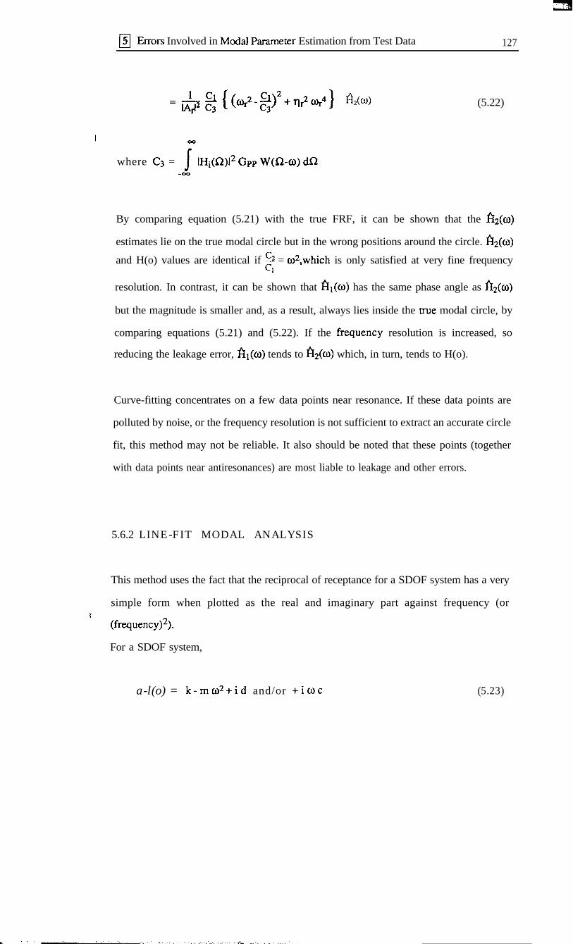
05 Errors Involved in Modal Paramgter Estimation from Test Data 127
(5.22)
where C3 = IHi( Gpp W(Q-a) dR
By comparing equation (5.21) with the true FRF, it can be shown that the &(co)
estimates lie on the true modal circle but in the wrong positions around the circle. &(a)
and H(o) values are identical if 2 = o2,which is only satisfied at very fine frequency
resolution. In contrast, it can be shown that Al(@) has the same phase angle as &(o)
but the magnitude is smaller and, as a result, always lies inside the true modal circle, by
comparing equations (5.21) and (5.22). If the frequency resolution is increased, so
reducing the leakage error, Al(w) tends to AZ(W) which, in turn, tends to H(o).
Curve-fitting concentrates on a few data points near resonance. If these data points are
polluted by noise, or the frequency resolution is not sufficient to extract an accurate circle
fit, this method may not be reliable. It also should be noted that these points (together
with data points near antiresonances) are most liable to leakage and other errors.
5.6.2 LINE-FIT MODAL ANALYSIS
This method uses the fact that the reciprocal of receptance for a SDOF system has a very
simple form when plotted as the real and imaginary part against frequency (or
’ (frequency)2).
For a SDOF system,
a-l(o) = k-m&+id and/or +ioc (5.23)

q5 Errors Involved in Modal Pammeter Estimation from Test Data 128
If Re (a-*(u)) is plotted against 02, then the result is a straight line whose intercept on
the frequency axis gives the resonance frequency and whose slope gives the effective
mass. If Im (a-l(o)) is plotted against o, then the slope of the line indicates the
magnitude of the viscous damping and the intercept on the magnitude axis gives the level
of structural damping. This technique can be extended to MDOF systems by subtracting
the effects of other modes before performing the analysis.
This method is useful for modes with insufficient data for circle-fitting, and is less
sensitive to leakage errors than is circle-fitting because the data used are away from the
immediate resonance region and the leakage error becomes maximum at the region and
decreases very rapidly as the frequency moves away from resonance.
5.7 NUMERICAL CASE STUDIES
To investigate measurement errors - such as the mass loading effects of transducers,
shaker/structure interaction, signal conditioning errors, signal processing errors etc. - on
FRFs, a computer program has been written which can simulate the various measurement
errors described above (Appendix E).
The test structure used in the following examples is a beam shown in Fig.5.12. The
structure was considered to be “excited” at a free end of the beam by a shaker whose
armature mass was 20 g. Periodic random excitation was “applied” throughout these case
j studies except in the case of leakage in which case pure random was also used for
comparison. The response of the structure was “measured” using an accelerometer whose
mass was 20 g. A force transducer of 10 g was assumed to “measure” input force. A
two-channel FFI analyser which has 801 lines of frequency resolution was used to
obtain frequency response functions.The frequency range of interest was 0 - 800 Hz.

151 Errors Involved in Modal Parameter Estimation from Test Data 129
p,= 7800 kg/m3 p2= 1%OOk&m’ p3= 7800 kg/m’
E, = 2.(@xlO”N/m* E$= 205klO”N/m* &= 4.18xlO”N/r11*
Fig.5.12 Beam Structure
Input and output noise was assumed to be white noise. The ratio of the noise spectrum to
the signal spectrum, r, which is defined as
where Gs is a signal spectrum, GN is a noise spectrum and Gs which is defined by
was assumed to be 10m3 for the input(force) signal and lOA for the output(response)
k? signal. The autospectra of input and output signals - noise free - and random noise are
shown in Fig.5.13.

cl5 Errors Involved in Modal Parameter Estimation from Test Data 130
SO.‘
0” 1a.c
i?
P“p -30.8
-79.0
-110.01.
,
I
LE-03
I- I- ------___. -
Fig.5.13 Autospectra of Input and Output Signals & Noise
5.7.1 MASS LOADING EFFECT
To investigate the mass loading effect of an accelerometer, the mass of the accelerometer
was increased from 20 g to 100 g. The natural frequencies of all modes decreased
(Fig.5.14). The natural frequency of the 6th mode decreased most because this mode has
the smallest apparent mass, while that of the 5th mode hardly changed because that mode
has the largest apparent mass.
i. ~ ,, I ._. _.i. ,. . . ,.

05 Errors Involved in Modal Parameter Estimation from Test Data 131
i.
-~ei~=i160. ate. 480. 6-8. 888.
W-RxQu- tnx,
Fig.5 14 Mass Loading Effect
5.7.2 SHAKER/STRUCTURE INTERACTION
From equation (5.4), it can be shown that the force spectrum near a resonance is given by
GFF(~) =GPP
1 + d A?
rl:
if Ar is assumed to be real. The amplitude of the force spectrum at resonance decreases as
the armature mass of the shaker increases - approximately proportional to the inverse
square of m, - as shown in Fig.5.15. The resulting FRFs are compared in Fig.5.16. Theti
only differences are around resonances, where the heavier armature mass makes the
coherence drop.
r .“S -. ._A’ ” _i _-

I
cl5 Errors Involved in Modal Parameter Estimation from Test Data 132
I -50.0 l.J!.-03 ! 168. 1 320. 488. 640.
I rmv- tnr,
Fid .15 Force SDectra
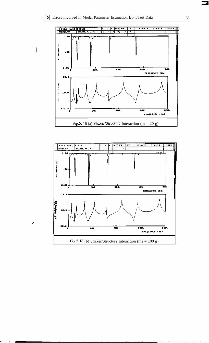
05 Errors Involved in Modal Parameter Estimation from Test Data 133
I-
F?
1.00
.50
0.00
50.0
18.8
-3Q.0a.
Fig-S. 16 (a) ShakedStmcture Interaction (m = 20 g)
Fig.5.16 (b) Shaker/Structure Interaction (ms = 100 g)

m Errors Involved in Modal Parameter Estimation from Test Data 134
i:
j
I.
I
I
5.7.3 RANDOM NOISE EFFECT
Usually, in modal analysis, only those FRF data near resonances are used to extract the
modal parameters. In these regions, HZ(~) reduces bias error from random noise because
r, may become negligible (equation (5.7)).
The output noise spectrum of i, = 10m4 , which may be achieved easily in random
excitation, is shown in Fig-S. 13 together with output signal spectrum. From Fig.5.17, it
can be seen that near resonances, where curve fitting is usually performed, the effects of
measurement random errors can be ignored. For example, near the 5th mode (fr = 309.8
Hz) which has maximum bias error, 304 Hz - 312 Hz, where curve fitting for the mode is
usually performed, the notmalised bias error is less than 4 % (0.06 - 3.2 %).
”12.9
:U
!;:
-46.0
-1tM.O1.
Fig.5.17 (a) Random Noise Effect (r, = 1O4)
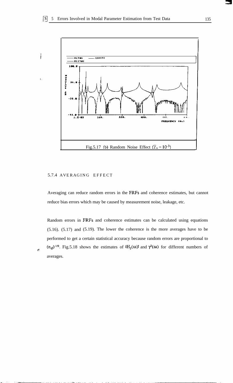
0 5 Errors Involved in Modal Parameter Estimation from Test Data 135
l.L-03 160. sac. 648. a m .
rnmumecv <WI>
Fig.5.17 (b) Random Noise Effect (m = 10e3)
5.7.4 AVERAGING EFFECT
Averaging can reduce random errors in the FRFs and coherence estimates, but cannot
reduce bias errors which may be caused by measurement noise, leakage, etc.
Random errors in FRFs and coherence estimates can be calculated using equations
(5.16). (5.17) and (5.19). The lower the coherence is the more averages have to be
performed to get a certain statistical accuracy because random errors are proportional to
r?(nd)‘tR. Fig.5.18 shows the estimates of IH,(o)l and y*(o) for different numbers of
averages.

05 Errors Involved in Modal Parameter Estimation from Test Data 136
1.&l- -If-
.59 --
\
40. tee. 400. 688. 688.
?lmQua?uY tnr,
Figs. 18 (b) Averaging Effect (nd = 100)

05 Errors Involved in Modal Parameter Estimation from Test Data 137 .;:,
5.7.5 LEAKAGE ERROR
i As discussed in sections 5.5.1 and 55.2, leakage causes deformation of the estimated!., spectra and therefore leads to bias
analysis is too coarse, compared with
errors in FRF estimates. If the resolution in the
the bandwidth of the resonances, the coherence can
iI detect this leakage by giving a value less than one around resonances and antiresonances,
as in Fig.5.19. The coherence therefore gives a warning of potential bias errors in the
FRF estimates. Fig.520 shows the relative error between true and estimated FRFs whichI
is affected by leakage. It can be seen that the most contaminated regions are near
resonances and antiresonances.
-50.8 !O.Q 8Q.Q 168.8 24Q.Q 22Q.Q 4t
~"SmCY <Hz,
Fig.5.19 Leakage Effect
.

05 Errors Involved in Modal Parameier Estimation from Test Data 138
-1RI701 - E R R O R 3-L217&31
I, 4m.ennmJuDux o(.B
Fig.5.20 (a) Relative Error (ERROR3) between True FRF (TR1701) andEstimated FRF (L21701)
-tRl791 - ERROR3
-Liz1781 IJB.B-
s_..--u.o--
Gg.5.20 (b) Relative Error (ERROR3) between True FRF (TR1701) and
Estimated FRF (L21701)

cl5 Errors Involved in Modal Parameter Estimation from Test Data 139
As discussed in section 5.6.1, &(o) is less sensitive to the leakage errors than is A,(O)
because F$(o) lies on the true modal circle (but in the wrong position). However, if the
frequency resolution is insufficient for a mode to encompass some part of the modal
circle, modal parameters extracted by circle-fitting may not reliable, as shown in
Fig.5.21.
O-FIT FOR MOPE 2)uTUIwL URrauMcy <HZ) = 61.4.sx DnNPxrtc ~STIWCTUML~ = -z.wseMOD. COHST. mc (l/RI) = ,658MOD. COUSI. m*sx (0) I -.3..42
Z WIDIUS WRIMIOH = .el
I-
Fig.5.2 1 Leakage Effect on Circle-Fit I
Fig.5.22 shows a Modified Line Fit analysis (or Bendent Method; see Appendin F) on
the 2nd mode. It can be seen that the effect of leakage is dominant only near resonance
and, therefore, has little effect on the extraction of modal parameters.

I
05 Errors Involved in Modal Parameter Estimation from.Test Data 140
L - T I T FOR 9WDI 29wTURaL FRmuMcy tnr> = ‘2.54
r: mwrm ~sTRucTuML) = .37?1K)D. COMST. mc Cl/)(U) = .191
Fig.5.22 (b) Estimated FRF

fl Errors Involved in Modal Parameter Estimation from Test Data 141
5.8 MODEL UPDATING OF BEAM STRUCTURE
The structure which featured in 0 5.7 was also used to check the validity of the IEM on a
!i practical structure which has realistic measurement errors. 20 beam elements were used to
create an analytical model of the structure and 2 DoFs - one translational and one
;, rotational DoFs - were considered at each node. Mass and stiffness modelling errors were
introduced by overestimating the density of the 1st and 2nd elements by 100 %I and the
Young’s Modulus of the 1 lth and 12th elements by 100 8, as shown in Fig.5.12.
A total of 11 points were “measured” in the vertical direction (Fig.5.23) using periodic
random excitation in the frequency range of 0 - 800 Hz with excitation applied at a free
I end of the structure. The ratio of noise to signal spectra was assumed to be 10e3 for force
and lOA for the response. An accelerometer of 20 g was moved from one location to the
next location in order to measure all FRFs. As a result, each measured FRF was expected
to have different mass loading effect.
Excitation
Fig.5.23 Measurement Points

05 Errors Involved in Modal Parameter Estimation from Test Data 142
Fig.5.24 shows one point and several transfer FRFs. In the measurement frequency
/ range, 8 flexible modes are clearly seen.I
I.
1
I
-DBfDlUl -DB178l -DBSSDl__ DBHYUI -D&?3Bl -DBUBl
1.6-03 160. 320. 6M. me.?xmux?tcv o(r>
Fig.5.24 Point FRF and Transfer FRFs
The modal parameters of an individual FRF were extracted by modified Line Fit analysis
using MODENT program [37]. All the identified modal parameters which exhibited
slightly different values (natural frequencies and modal dampings) were then collated to
obtain consistent modal parameters using MODESH [38]. The resultant parameters can be
r. seen in Table 5.4. The first 8 “experimental” and initial analytical natural frequencies are
compared in Table 5.5.
k

q5 Errors Involved in Modal Parameter Estimation from Test Data 143
Table 5.4 Modal Parameters of “ExDerirnental” Data_
Mode Min
1 22.92 62.23 126.34 208.65 308.26 438.17 567.28 749.0
Natural
23.062.8127.1210.2309.8441.2570.6753.4
FreqMean
23.062.6126.8209.7309.2440.2569.3751.7
SD
0.050.170.240.460.580.870.981.24
Min
0.980.540.510.500.500.500.510.50
1.090.600.540.530.530.520.510 . 5 2
Damping (so)
Mean SD
1.02 0.040.57 0.020.53 0.010.52 0.010.52 0.010.51 0.010.51 0.000.51 1 0.01
Table 5.5 Natural Freuuencies of “Experimental” and Initial Analvtical M&els
In the error location procedure, 5 macro elements were used and each macro element had
4 individual elements. The error location results are shown in Fig.5.25 and Table 5.6.
After 4 iterations, it became possible to locate possible error regions - 4 mass elements
and 12 stiffness elements.

cl5 Errors Involved in Modal Parameter Estimation from Test Data 144
H ; Selected Elements
-l!.... . . =. . - - =. . . . . . .2 4 6 8 1 0 12 14
(a) Mass Error
16 18 20Element Numbers
B ; Selected Elements
2 4 6 8 10 12 14 16 18 20Element Numbers
(b) Stiffness Errors
Fig.5.25 Error Location Results

Cl5 Errors Involved in Modal Parameter Estimation from Test Data 145
Table 5.6 Natural Frequencies of “ExtXrimentai” and Intermediate Analvtical Models
After locating possible error regions, the updating was carried out with the correction
coefficients calculated as initial values. It can be seen in Figs 5.26 and 5.27 that the
estimates became quite accurate after 5 iterations. The natural frequencies of the updated
analytical model are compared with the experimental ones in Table 5.7.
Table 5.7 Natural Freuuencies of “Experimental” and Undated Models
1 12 13 14 15 16 17 18
23.0 62.5 126.8 209.7 309.2 440.2 569.3 751.7
22.8 62.3 126.5 209.7 309.1 441.0 570.2 753.7
0.999 1.000 1.000 0.999 1.000 0.999 0.999 0.999 ‘
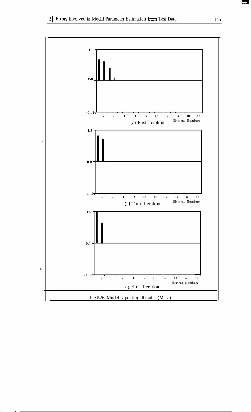
05 kors Involved in Modal Parameter Estimation from Test Data 146
1.5
0.0 I
- 1 . 5 . . . . . . . . . . . . . . . . , , . ,2 4 6 8 10 12 14 16 18 2 0
(a) First Iteration Element Numbers
1.5
0.0
- 1 . 5 . . * . . . - - - - - = . . . . . . . . t2 4 8 I) 10 12 14 16 18 2 0
(b) Third Iteration Element Numbers
1.5
0.0 -
- 1 . 5 . . - - . - - . = - - - - ’ - - - . . .t2 4 6 8 10 12 14 16 18 2 0
Element Numbers(c) Fifth Iteration
Fig.526 Model Updating Results (Mass)
L ,

q Errors Involved in Modal Parameter Estimation from Test Data 147
1.5
-1 .5 . . . . . . . . . . . . . r . . . . . .2 4 6 a 10 12 14
(a) First IterationE;:ment'~um~;
-1 .5 . . . * = . - . . . . . * . . . . . . .2 4. 8 6 10 12 14 16 16 2 0
(b) Third Iteration Element Numbers
1.5
0.0
-1 .5 . . . . . . . . r . . . . . . . . . . . \2 4 6 6 10 12 14 16 16 2 0
(b) Fifth IterationElement Numbers
Fig.5.27 Model Updating Results (Stiffness)
b

m Errors Involved in Modal Parameter Estimation from Test Data 148
5.9 CONCLUSIONS
The characteristics of typical measurement errors might not result in random variations in
i the modal parameters which are eventually derived from the measured data. For model
updating methods to be useful in practical application, various error sources in testing -
such as the mass loading effect of transducers, shaker/structure interaction, etc. - should
be considered and more realistic errors rather than random noise should be included in the
“experimental” data
The errors involved in modal parameter estimation - such as measurement errors, signal
processing errors and errors in modal analysis - have been investigated, and their effects
I on estimated FRFs and on the modal parameters extracted from the FRFs have also been
investigated. A computer program has been written to simulate various measurement and
signal processing errors. The “experimental” FRFs calculated using this program can be
used to test the performance of different modal parameter identification programs and,
thus, of the various applications to which these modal data are put.
The resultant “experimental” modal data which contained representative experimental
errors have been used to update the corresponding analytical beam model to check the
validity of the IEM. The mismodelled regions were located successfully, and the updating
results were found to be quite accurate, not only in modal parameters but also in
correction coefficients or physical design variables.
* 1.


q Updating of Damped structures 150
1 CHAPTER 6
i, UPDATING OF DAMPED STRUCTURES
I 6.1 PRELIMINARIES
In the previous Chapters, location of mismodelled regions in an analytical model and
updating the model were carried out using corresponding experimental modal data which
were all real (i.e. for undamped systems). However, in most cases, experimental modal
data from a real structure are not real but complex, even if the structure is lightly damped.
If a structure is lightly damped, the modal data from measurement are often treated as real
modes, and the method suggested in Chapter 3 can be used to update the corresponding
analytical model. However, some practical structures are more heavily damped and the
measured modal data cannot be regarded as real, whereas the modal data from the
corresponding (undamped) analytical model are real.
There are two possible approaches to resolve this incompatibility. One approach is to
r deduce the undamped modes - real modes - from the measured complex modes
[19,39,40]. Then the method suggested in Chapter 3 can be used to update the analytical
model using the deduced real modes. However, the deduced real modes are often only a
rough approximation because the experimentally identified complex modes are incomplete
and the deduction itself relies on the analytical model which is erroneous.

m Updating of Damped Structures 151
An alternative approach is to use the experimental complex modes directly to update the
analytical model. A method has been developed by He [17] to locate the damping
i. elements in an analytical model using measured complex modes. However, this method
requires a complete set of measured coordinates, which is not practical, or the use of
, mode expansion, which may be an erroneous procedure thus jeopardising exact location,
in order to overcome the incompatibility between the measured modes and the analytical
model. In this Chapter, a complex inverse eigensensitivity method will be introduced to
1 locate and to update the damping elements together with the mass and stiffness elements
which have modelling errors, using measured complex modal parameters.
6.2 COMPLEX EIGENSENSITIVITY
The updated damping matrix can be expressed as equation (6.1) in the same way as the
mass aid stiffness matrices in equation (3.1) and (3.2)
(6.1)
where L is the number of elements, ci are correction coefficients to be determined and ~1;
is a submatrix of the system damping matrix.
The governing equations of motion for a MDOF system with structural damping and no
extemai forcing can be written in matrix form as:r
Ml(i) + [Kl(x) +i PI(x) = (0)
By assuming a solution of the form:
(6.2)
. ,

B Updating of Damped Structures 152
(x) = (x } eip'
i we can obtain a complex eigenpmblem
where (@), is normal&d such that
(6.3)
(6.4)
! The solution of this eigenproblem is in the form of two matrices containing complex
eigenvalues and complex eigenvectors in contrast with the undamped case where
eigenvalues and eigenvectors are all real.
Differentiating equation (6.3) with respect to updating variable pi gives
arD1+ i api - apia[Ml%W - hr-api woW,+Wl +iPl -IqlMl)--gf = (0)
(6.5)
Pm-multiplying equation (6.5) by (Q)T leads to
(6.6)
The eigenvector derivatives can be expressed as linear combinations of all eigenvectors of
the system if the eigenvalues are assumed distinct, because N eigenvectors are linearly
independent and they can be used as a set of bases vectors for spanning N-dimensional
’ space. Thus,

m Updating of Damped Structures 153
?* = i ajj($)ji j-l
(6.7)
!,’ Substituting equation (6.7) into equation (6.5) and pre-multiplying equation (6.5) by
r44:,,
If k#r,
Thus,
ajk =awl aux+ i api - A, api
%- hc
aA C~II be obtained by differentiating equation (6.4) with respect to pi
r Substituting equation (6.7) into equation (6.11) leads to
(6.9)
(6.10)
(6.11)
(6.12)

i
q UpdatingofDampedStructures : 154
From equations (3-l), (3.2) and (6. l), we get
XWx = [Wi
arKi-q- = lOI
a[Ml- = [O]abi
arKIq = rKJi
Pi = m
Substituting equation (6.13) into equation (6.6) leads to
n
and substituting equation (6.13) into equations (6.10) and (6.12) leads to
?p = t ajj($)ji j=l
i-
1, (@IiT [Mli (@I, bWa3 = h,- hj
1- 2 I@ljT [Mli IQ), (r=j)
{$)iT [‘Ii ($1,pj = h,- hj
0
W.0
(r=j)
(6.13)
(6.14a)
(6.14b)
(6.14~)
(6.15a)
(6.15b)

q Updating of Damped structures 155
F = 2 y;j($)ji j=l
y’. =rJ
i I$liTIDli ($1,or- ~j
(r#j >
(6.15~)
(r=j>
If we assume that the element damping matrix has the same distribution as the element
stiffness matrix, i.e.,
, (noting that this assumption is not the same as [D] = a[K], which is “proportional”
damping, since the modal parameters generally remain complex under the assumption
[D]i = a IK]i), then a complex stiffness mtxix [K*] which is defined as:
[x*] E [K]+ip] = i bi [K]; + i i ci [D]ii=l i=l
can be expressed as:
@*] = i (bi + i a Ci) [K]ii=l
= ~ b~[K]ii=l
I’- wherebf=bi+iac.1
Therefore,

q Updating of Damped Structures 156
Substituting equation (6.13) and (6.16) into equation (6.6), (6.10) and (6.12) leads to
y = 2 PjjC+)ji j=l
Icp)iT rq Ml, (r*j 1pi. =rJ h,- 3Lj
0 (r=_i)
The first-order Taylor expansions of the modal parameters can be written as:
or
‘Aat..
A aLAb;
.
.
.!Ab;.
(6.16a)
(6.16b)
(6.17)
(Al m(n+l) x 1 = PI m(n+l) x 2L fAPJ2L x 1
which is very similar to equation (3.23). However, in equation (6.17), {A), [S] and
{Ap) are not real, as in equation (3.23), but complex. The real parts of ai (i = 1,2,..., L)
represent mass correction coefficients and the real parts of by (i = 1,2,..., L) represent

q Updating of Damped Srn~ctures 157
stiffness correction coefficients, while the imaginary parts of bi represent damping
correction coefficients.
The correction coefficients vector (Ap) can be calculated as:
I UP) = ([SIT PI)-' [SIT (A)
then, ( Ap) is added to the solution vector to update the vector
(PI new = {P]cta + (AP]
(6.18)
(6.19)
’ and the process is iterated until convergence is achieved.
6.3 APPLICATION TO THE BAY STRUCTURE
The structure which had been used in previous Chapters (Fig.2.2) was used again to
check the validity of the method proposed above. The structure is modelled by 31 beam
elements, and 3 DoFs are considered at each node, so that the total number of DoFs (N)
is 90. Experimental data were obtained at 15 points as shown in Fig.2.2 in translational
coordinates only (i.e. n = 30). The first 10 experimental modes were used (i.e. m = 10).
Mass and stiffness modelling errors were introduced by overestimating the mass matrices
of the 25th and 26th elements by 50 % and the stiffness matrices of the 12*, 13th and 31st
” elements by 100 %. In addition, the lst and 2”d elements were supposed to have damping
of [Dli = 0.05 [K]; (Case 1; lightly damped case) and of [D]i = 0.3 [K]i (Case 2; more
heavily damped case).

q Updating of Damped Structures 158
6.3.1 CASE 1
iIt should noted that the modal parameters of the ‘analytical’ model (undamped) are real
while those of the ‘experimental’ version are complex because this system is damped.
The modal parameters of the fust 10 ‘experimental and analytical modes are compared in
, . Table 6.1 together with MAC values. For complex modes, MAC can be expressed as:
It should be noted that the MAC values are still real even if mode shapes are complex.
, The eigenvectors of the first two ‘experimental’ and analytical modes are compared in
Tables 6.2 and 6.3.
Table 6.1 Natural Frequencies of ‘Ex_perimental’ and Analvtical Models (Case 1)
Mode Experimental AIMlytiCd MAC
No. Nat. Freqs. Loss Factors Nat. Freqs. Values
1 343.3 0.003 342.3 0.995
2 468.1 0.002 450.6 0.97 1
3 548.2 0.012 528.5 0.948
4 577.7 0.002 557.2 0.966
5 704.4 0.007 683.4 0.960
6 850.9 0.004 833.7 0.98 1
7 917.2 0.003 902.3 0.914
8 928.9 0.000 927.0 0.814
9 1099.4 0.002 1066.6 0.862
10 1205.0 0.006 1165.3 0.927

q Updating of Damped Stmctures 159
Table 6.2 Eigenvectors of ‘Extmirnental’ and Analytical Models (Case 1: Mode 11
Coords Exp.(xlO-‘)
1 0.723(0’)
2 0.260(0’)
7 0.355(0°)
8 0.260(0’)
13 0.134( 175O)
14 O-234(0’)
19 0.578( 180”)
20 0.193(0”)
22 0.733( 180’)
23 0. 176(O”)
28 0.717(180”)
29 D.016(-177°)
37 3.725(- 179’)
38 X243( 180’)
40 1.651(180’)
Anal.(xlO1)
0.748(0’)
0.236(0’)
0. 370(0°)
0.248(0”)
0.134( 180”)
0.233(b”)
0.593( 180”)
0.205(0’)
0.754( 180”)
0.1 92(O”)
0.742( 1 SO”)
0.019( 1.80”)
0.748( 180”)
0.236( 180”)
X585( 180”)
Coords Exp.(xlO-‘)
41 0.253( 180”)
46 0.202( 180”)
47 0.254( 1 SO”)
52 0.3 16(0”)
53 0.231(180°)
58 0.726(0’)
59 0.205( 180’)
67 0.715(0°)
68 0.080(2°)
76 0.406(- 1”)
77 0.1 54(0°)
82 0.159(-179”)
83 0.415(-178’)
88 0.648( 180”)
89 X222( 1 SO”)
Anal.(xlO-1)
0.246( 180”)
0.123(180”)
0.244( 180’)
0.380(0”)
0.220( 180”)
0.754(0”)
0.192(180°)
0.740(0”)
3.072(0’)
X398(0’)
I.121(0°1
>.138(180”)
X420( 180’)
).610(180°)
).188(180”)
. ._ ,. dL ,. :

q updating of Damped Smmwes 160
Table 6.3 Eieenvectors of ‘Exoerimental’ and Analytical Models (Case 1: Mode 2)
Coords. Exp.(xW)I
Anal.(xlO-‘)
2
7
8
13
14
19
20
22
23
28
29
37
38
40
0.058(-176”) 0.008(180”)
0.046( 173’) 0.024( 180’)
0.459( 177O) 0.353( 180”)
0.047( 175’) 0.033( 180”)
0.579( 178’) 0.496( 180”)
0.102(179°) 0.097(180°)
O-342( 179’) 0.354( 180”)
0.188(180”) 0.195(180”)
0.129(-177’) 0.196(180”)
0.238(180’) 0.250( 180’)
0.043(-173’) 0.102(180°)
0.192(-179’) 0.223(180”)
0.034(-7O) 0.008( 18OO)
0.024(- 164”) 0.024( 1 SO”)
0.064(-175”) 0.195(180”)
Coords. Exp.(xlO’)I
Anal.(xlo-1)
41
46
47
52
53
58
59
67
68
76
77
82
83
88
89
0.017(-160’) 0.020(180”)
0.389(- 178”) 0.459( 180’)
0.053(- 175’) 0.060( 180’)
O-476(- 179’) 0.459( 180’)
0.145(-179’) 0.143(180°)
0.269(180”) 0.196(180°)
0.265( 180”) 0.250( 180’)
0.117(-179°) 0.061(180”)
0.207( 179’) 0.172( 180”)
1.289(0’) 1 .220(O” j
0.786(0’) 0.738(0’)
1.410(0°) 1.520(0’)
0.850(0’) 0.926(0’)
0.387(0”) 0.669(0”)
0.206( 1”) 0.399(0”)

q Updating of Damped Structures 161
The Macro 1 model (Fig.3.3) which has 8 macro elements (i.e. L = 8) was used in the
error location procedure. This means that no macro element coincided exactly with any of
the error regions. A necessary condition for the sensitivity [S], which is m(n=l) x 2L, toi be rank full is:
> m(n+l)>2L or rn>-$l
However, the eigenvector sensitivities are not always linearly independent. In practice,
’ the number of measured modes should be more than twice of the minimum number in
order to give a high probability of sufficient rank to matrix [S]. In this case study, 10
modes were used as mentioned above.
The location process took 5 iterations to convergence and 27 elements - 9 mass elements,
11 stiffness elements and 7 damping elements - were identified as possible error regions
as shown in Fig.6.1.
The resultant natural frequencies of the ‘improved’ analytical model are compared with
those of the ‘experimental’ modes in Table 6.4.
Table 6.4 Natural Frequencies of ‘Experimental’ and Intemnediate Models (Case 11

q Updating of Damped Structures 162
I0.5
0.0 ,,,,lll”“‘---‘nrr”‘~n 1111
1 ; Selected Elements
- 0 . 5 *. *. . . *. * *. * *. *.. . . . . . . - *. . . . ..’2 4 6 8 IO 12 14 16 I8 20 22 24 26 28 30
(a) Mass Modelling ErrorsElement Numbers
I
0 11111 I . . . . . . . . .
1; Selected Elements
-I...........*....,..‘.‘.‘.......’2 4 6 8 IO I2 14 16 18 20 22 24 26 28 30
(b) Stiffness Modelling ErrorsElement Numbers
005-
-005.-......,......................~2 4 6 8 lo I2 I4 I6 I8 20 22 24 26 28 30
Element Numbers
(c) Damping Modelling Errors
Fig.6.1 Error Location Results
L

q Updating of Damped Structures 163
Using the error location results, updating was carried out by correcting the selected errors
in the original analytical model. The iteration results of this stage are shown in Figs.6.2,
6.3 and 6.4, from which it can be seen that the final estimates become very accurate after
’ 5 iterations. Natural frequencies of the updated model are compared with ‘experimental’
natural frequencies together with MAC values in Table 6.5.
Table 6.5 Natural Freuuencies of ‘Experimental’ and Uodated Models

q Updating of Damped Structures 163
Using the error location results, updating was carried out by correcting the selected errors
in the original analytical model. The iteration results of this stage are shown in Figs.6.2,
6.3 and 6.4, from which it can be seen that the final estimates become very accurate after
’ 5 iterations. Natural frequencies of the updated model are compared with ‘experimental’
natural frequencies together with MAC values in Table 6.5.
Table 6.5 Natural Freuuencies of ‘Experimental’ and Urxiated Models
. 2..

q Updating of Damped Structures 164
0 II I I II
-l...............................2 4 6 8 10 12 14 16 18 2 0 22 24 26 28 30
(a) Mass Modelling Emrs Element Numbers
2
0 . Ill .I
w
-2.................................2 4 6 8 10 12 14 16 18 20 22 24 26 28 30
(b) Stiffness Mdelling Errors Element Numbers
0.1
-0.1.. * . . . . . -. - -. " - ". -. . . . -. . . ..-2 4 6 8 10 12 14 16 18 2 0 22 24 26 28 30
Element Numbers(c) Damping Modelling Errors
Fig.6.2 Model Updating Results (Case 1; First Iteration)
.’ ,._ ___~

q Updating of Damped Structures 165
l-
-l...............................2 4 6 8 10 12 14 16 18 20 22 24 26 28 30
(a) Mass Modelling Errors Element Numbers
2
0 I
- 2 . . . m..... ..*..... .I............2 4 6 8 10 12 14 16 18 20 22 24 26 28 30
(b) Stiffness Modelling Errors Element Numbers
0.1
0
-0.12 4 6 8 10 12 14 16 18 2 0 22 24 26 28 3 0
Element Numbers(c) Damping Moclelling Errors
Fig.6.3 Model Updating Results (Case 1; ‘IKrd Iteration) I

q Updating of Damped Structures 166
t
0
-l......=. - -. - "' - '. ' - - '1 1 " - '-. '2 4 6 8 10 12 14 16 18 2 0 22 24 26 28 30
(a) Mass Modelling J3rors Ekment Numbers
0
LJ
-2!.. ...~....."...“‘.,."""', 72 4 6 8 10 12 14 16 18 2 0 22 24 26 28 30
(b) Stiffness Modelling Errors Ekment Numbers
.
2 ,
L
2 4 6 8 10 12 14 16 18 2 0 2 2 2 4 2 6 2 8 3 0Element Numbers
(c) Damping Modelling Errors
Fig.6.4 Model Updating Results (Case 1; Fifth Iteration)

q Updating of Damped Structures 167
6.3.2 CASE 2
For the more heavily damped case, the damping properties in the la and 2nd elements
k were increased to 0.3 [K]i. The modal parameters of the first 10 ‘experimental’ and
analytical modes are compared in Table 6.6 together with h4AC values. The eigenvectors
] , of the first two ‘experimental’ and analytical modes are compared in Tables 6.7 and 6.8.
/ Table 6.6 Natural Freuuencies of ‘ExDerirnental’ and Analvtical Models (Case 2)
mde
No.
1
2
3
4
5
6
7
8
9
10
Experimental AIldytiCd MAC
Nat. Freqs. Loss Factors Nat. Freqs. Values
344.3 0.019 342.3c
0.992
469.2 0.013 450.6 0.967
552.1 0.07 1 528.5 0.927
578.5 0.013 557.2 0.960
704.7 0.043 683.4 0.948
852.8 0.024 833.7 0.978
918.7 0.018 902.3 0.885
928.9 0.002 927.0 0.79 1
1100.5 0.010 1066.6 0.854
1206.2 0.038 1165.3 0.890
e.’

q Updating of Damped Structures 168
Table 6.7 Eieenvectors of ‘Exmimental’ and Analvtical Models 0se 2: Mode 1)
Chords.I
Exp.(xlO-‘)I
Anal.(xlO’)
1 0.717(-2”)
2 0.259(2O)
7 0.379( 12’)
8 0.262( 1”)
13 O.l17(153O)
14 0.235( lo)
19 O-574( 178’)
20 0.194(1°)
22 0.735( 180”)
23 0.177(1°)
28 0.719(180°)
29 0.017(-167°)
37 0.727( 180”)
38 0.247(-177’)
40 0.653(-179”)
0.748(0’)
0.236(0”)
0. 370(0°)
0.248(0’)
0.134( 180’)
0.233(0’)
0.593( 180”)
0.205(0’)
0.754( 180’)
0.1 92(O”)
0.742( 180’)
0.019(180°)
0.748( 180”)
0.236( 180”)
0.585( 180’)
Coords Exp.(xlO’)
41
46
47
52
53
58
59
67
68
76
77
82
83
88
89
0.256(- 178’)
0.204(-178’)
0.255(-179”)
0.315(-lo)
0.231(180°)
0.730(0”)
0.203( 177”)
0.71 l$lO)
0.084(8”)
0.399(-4O)
O-153(-2’)
0.166(-172’)
0.452(-173’)
0.652(- 179’)
0.227(- 177’)
Anal.(xlO’)
0.246( 180”)
0.123(180”)
0.244( 180”)
0.380(0”)
0.220( 180’)
0.754(0”)
0.192( 180’)
0.740(0”)
0.072(0”)
0.398(O”j
0.121(0°)
0.138(180”)
0.420( 180”)
0.610(180”)
0.188(180”)
L. ,“.

q Updating of Damped Structures 169
Table 6.8 Ekenvectors of ‘Exuerimental’ and AnahticaI Models K&e 2: Mode 2)1
Coords. Exp.(xlO-‘) Anal.(xlO’) Coords. Exp.(xlO’) Anal.(xlO1)
1 0.064(-162”) O.OOS( 180’) 4 1 0.027(-l 29”) 0.020( 180”)
2 0.035( 140”) 0.024( 1 8 0 ”) 4 6 0.412(-173’) 0.459(180”)
7 0.411(163’) 0.353(180”) 4 7 0.060(-158”) 0.060( 180”)
8 0.041(154°) 0.033(180”) 5 2 0.493(-175’) 0.459( 180”)
13 0.542( 169’) 0.496( 1 SO”) 53 0.149(-175’) 0.143(180”)
14 o.100(171°) 0.097(180”) 5 8 0.270(180”) 0.196(18G”)

q Updating of Damped Structures 170
The same macro model as that of Case 1 was used for error location. It took 6 iterations
to converge and 27 elements - 9 mass elements, 11 stiffness elements and 7 damping
1’ elements - were identified as possible error regions, as shown in Fig.65
The resultant natural frwluencies of the ‘improved’ analytical model are compared with
those of the ‘experimental’ modes in Table 6.9.
Table 6.9 Natural Freuuencies of ‘ExDerimental’ and Intermediate Models (Case 2)
c

q Updating of Damped Structures 171
.I-
2 4 6 8 10 12 14 16 18 20 22 24 26 28 3C
(a) Mass Modelling Errors Element Numbers
I
0
-1
I I I I ID I _ I
l_l1 ; Selected Elements
,2 4 5 8 IO I2 14 15 :o 30 - 22 24 26 28 30
(b) Stiffness Modelling Errors Element Numbers
0
-0.2
j/
Ll1 1 ; Selected Elements
2 4 6 8 IO 12 14 I6 I8 20 22 24 26 28 30Element Numbers
(c) Damping Modelling Errors
Fig.6.5 Error Location Results (Case 2)

q Updating of Damped Structures 172
Using the error location results, updating has been carried out. The iteration results are
shown in Figs.6.6,6.7 and 6.8, fkom which it can be seen that the final estimates become
very accmte after4 iterations.
Natural frequencies of the updated model are compared with ‘experimental’
] frequencies together with MAC values in Table 6.10.
natural
I Table 6.10 Natural Freuuencies of ‘ExDerimental’ and Undated Models (Case 2)
c
*.

q Updating of Damped Structures 173
0 . I . I I
-l!..............................2 4 6 8 1 0 12 14 16 1 8 2 0 2 2 2 4 2 6 2 8 3 0
(a) Mass Moclelling Eh-ors Element Numbers
2
f
0 . I II rn n
-2............................,....,2 4 6 8 10 12 14 16 18 20 22 24 26 28 30
0.5
0.0
-0.5
(b) Stiffness Modelling ErrorsEiement Numbers
I_I.
2 4 6 8 1 0 12 14 16 18 2 0 2 2 2 4 2 6 2 8 3 0Etemeat Numbers
(c) Damping Mdelling Errors
Fk.6.6 Model Umiating Results Case 2: First Iteration)

q Updating of Damped Structures 174
1
1
0
-1 l-+2 4 6 6 10 12 14 16 18 2 0 22 24 26 28 30
(a) Mass Modelling Errors Element Numbers
2
0
-2!.............................. ‘I
2 4 6 8 10 12 14 16 18 20 22 24 26 28 30
(b) Stiffness Mdelling Errors Element Numbers
0.5
0.0 -*
I
-0.5!m......... . . =. .". =. . . . . . *. . . . . ,
2 4 6 8 10 12 14 16 18 20 22 24 26 28 30Element Numbers
(c) Damping Modelling Errors
Fk6.7 Model Udatinrr Results (Case 2: Third Iteration)
I

m updating of Damped Structures 175
-1. * . . . . . . . . . . . . . . . . . . . . . . . . . . . . . .2 4 6 8 10 12 14 16 18 20 22 24 26 28 30
(a) Mass Modelling Emrs Element Numbers
2 ,
0
a ! . . . . . . . . . . . . . . . . . . . . . . . . . . . . . . .2 4 6 8 10 12 14 16 18 20 22 24 26 28 30
(b) Stiffness Modelling ErrorsElement Numbers
V.” I
0.0 -*
L-.-Jx).5......... *. - - ' -. ". *. - =. . . . . . . -
2 4 6 8 10 12 14 16 18 20 22 24 26 28 30Element Numbers
(c) Damping Mdelling Errors
Fig.6.8 Model Updating Results (Case 2; Forth Iteration)
* ‘.d_

q Updating of Damped Structures 176
6.4 CONCLUSIONS
The damping properties of most vibrating structures are not distributed in a similar way to
i’ the mass or stiffness. Rather, damping often results from the joints between various
components of a structure. As a result, measured modal data are often complex, while the
modal parameters of the corresponding analytical model are real.
Updating methods developed so far generally assume that the experimental modal data are
I red, or postulate that the measured complex data have successfully been converted to real
data. However, the deduced real modes may be erroneous because the experimentally-
identified complex modes are incomplete and the deduction itself relies on the analytical
I model which is erroneous.
A method has been developed to locate and to update damping elements together with
mass and stiffness elements in analytical model using measured complex modal data The
proposed method has been applied to the free-free bay structure which may constitute a
realistic problem in respect of the incompleteness of both measured modes and
coordinates. The updating results are quite accurate not only in modal parameters but also
in correction coefficients namely, physical design variables.

3

cl7 Conclusions 178
i CHAPTER 7
CONCLUSIONS
’ 7.1 GENERAL CONCLUSIONS
Due to advances in numerical methods and the availability of powerful computing
facilities, FE modelling has become the most popular technique in structural dynamic
analysis. However, the dynamic responses obtained from FE analysis are seldom in
perfect agreement with modal testing results. Therefore a model updating procedure
should be introduced in order to adjust the analytical model so that the analysis and test
results agree, and so that a valid model is available for design calculations.
It should be noted that modal parameters obtained from a modal test are generally not
fully compatible with those from the analytical model because
1)
7; 2)
3)
the number of modes available from measurement (m) is usually very
limited (m-2 < N),
the number of measured coordinates (n) is in genera-l much less than the
number of coordinates (or the number of degrees of freedom) of an
analytical model (nfl) and
in most cases, experimental modal data from a real structure are not real but

F7l Conclusions 179
complex, even if the structure is lightly damped, while the modal parameters
of the corresponding analytical model are real.
Any incompatibilities between measured modes and the analytical model should be,
resolved before an updating procedure is applied, or alternatively, an updating method
should be used which can handle the incompatibilities.
Various methods have been proposed to improve an analytical model of a mechanical
structure using modal test results. Review and numerical studies have revealed someI inherent problems of those methods. One of the main problems of direct updating
methods, such as function minimisation methods and the error matrix method, is that the
updated model is a numerically-optimised one rather than a physically-meaningful model.
As a result, the modes outside frequency range of the experimental data remain
questionable or may become even worse than those of the original analytical model.
Another problem with these methods is that mode expansion is often required in order to
overcome the inevitable incompatibility between the analytical model and the measured
modes. This might itself be an erroneous procedure, thus jeopardising the subsequent
model updating. On the other hand, iteration methods such as IEM which do not require
such expansion usually do not converge if the modelling errors are not small.
Any attempt to update every element in the analytical model using only the limited
information available from typical test results may not be realistic. If mismodelled regions
can be located in a preliminary step, model updating can be carried out more efficiently
and more successfully. Therefore, error location is a fundamental first objective of the
updating process. Recent developments in the area of error location have beeni‘I; investigated. The EMM can locate mismodelled regions successfully even with a very
limited number of measured modes if complete coordinates are measured, although this is
not a very practical proposition. Again, for the EMM to be successful, a reliable mode
expansion method should be available. The IEM does not require mode expansion and its
computational time will be reduced by locating error regions first and updating the

l-l7 Conclusions 180
analytical model using only the elements which are selected in an error location
procedure. However, the IEM had been found to be unreliable from case studies in
Chapter 2, from which it was concluded that more reliable error location methods needed
1 to be developed.
The objectives of this research were decided based on these findings, and were:
1) to develop a reliable, sensitive and systematic method to locate modelling
errors in an analytica.l model using modal testing results, and
2) to develop an updating method which can produce an improved analytical
model that can not only reproduce the exact modal parameters measured in a
test but also predict correctly those modes outside frequency range of the
experimental data and at the same time can reduce the number of experimental
modes and the computational time for updating.
An inverse eigensensitivity method using arbitrarily-chosen macro elements has been
proposed at the error location stage to reduce the computational time and to reduce the
number of experimental modes required for subsequent updating. By this approach, the
model updating problem, which is generally under-determined, can be transformed into
an over-determined one and an updated analytical model can be found which is not
influenced by the definition of the macro elements. The proposed method has been
applied to the free-free GARTEUR structure which represents a practical structure and
constitutes a realistic problem in respect of the incompleteness of both measured modes
and coordinates. The updating results were quite accurate, not only in modal parameters
but also in correction coefficients for the physical design variables.
The assumption that the test results represent the true dynamic behaviour of a test
structure, however, may not be correct. Experimental data can be affected by several
typejof measurement error in spite of the highly-developed instrumentation and modal
parameter extraction techniques now available. Thus, the sensitivity of the updating

07 Conclusions 181
method itself to noise on the experimental data needs to be investigated. The proposed
method has been applied to a Bay structure for which “experimental” data are noisy and
incomplete. The error location procedure has been found to be very insensitive to the
I “measurement” errors - in the presence of measurement errors of up to 1 % in the
eigenvalues and 10 % in the eigenvectors, it succeeded in locating the correct
mismodelled regions. The updating results were quite accurate in terms of modal
parameters and, moreover, in terms of correction factors, when sufficient eigensensitivity
terms ate used. In this case study, measurement errors were introduced by contaminating
, the modal parameters of the correct or modified structure with random noise.
In practice, the characteristics of measurement errors might not result in random
variations in the modal parameters. For the updating method to be useful in practical
application, various error sources in testing - such as the mass loading effect of
transducers, shaker/structure interaction, etc. - should be considered and more realistic
errors rather than random noise should be included in the “experimental” data. The errors
involved in modal parameter estimation - such as measurement errors, signal processing
errors and errors in modal analysis - have been considered in detail, and their effects on
estimated FRFs and on the modal parameters extracted from the FRFs have also been
investigated. A computer program has been written to simulate various measurement and
signal processing errors. The “experimental” FRFs generated using this program can be
used to test the performance of different modal parameter identification programs and,
thus, of the various applications to which these modal data are put.
The resultant “experimental” modal data which contained representative experimental
7; errors have been used to update the corresponding analytical beam mtiel to check the
validity of the IEM. The mismodelled regions were located successfully, and the updating
results were found to be quite accurate, not only in the modal parameters themselves but
also in correction coefficients for the physical design variables.
: I,._,“,d* ._I.,,.. _...- ..__ , .,_ .:..._.. ,, -._ ._

q7 Conclusions 182
The damping properties of most vibrating structures are not distributed in a similar way to
the mass or stiffness. Rather, damping often results from the joints between various
components of a structure and, as a result, measured modal data often are complex, while
!. the modal parameters of the corresponding analytical model are real. Updating methods
developed so far assume that the experimental modal data are real, or postulate that the
measured complex data have successfully been converted to real data. However, the
deduced real modes may be erroneous because the experimentally identified complex
modes are incompatible and the deduction itself relies on the analytical model which is
1 erroneous.
A method has been developed to locate and to update damping elements together with the
mass and stiffness elements in an analytical model using measured complex modal data.
The proposed method has been applied to the free-free Bay structure, constituting a
realistic problem in respect of the incompleteness of both measured modes and
coordinates. The updating results were quite accurate, not only in modal parameters but
also in correction coefficients namely, physical design variables, which means that this
method can handle all the inherent incompatibilities between measured modes and an the
analytical model.

f-l7 Conclusions 183
7.2 CONTRIBUTIONS OF THE PRESENT RESEARCH
As a final review, the contributions of this research are listed chapter by chapter so that it
! becomes clear which parts of the work constitute new developments to the subject.
,
Chapter 2 - Model Updating Methods - A Review
I l
.
.
review of various updating methods and critical discussion on their advantages and
disadvantages/limitations.
discussion on incompatibility between measured modes and an analytical model
and, on the solutions to their problems
review of various error location methods and critical discussion on their advantages
and disadvantages/limitations, especially on the IEM based on some numerical case
studies
Chapter 3 - Model Updating Using IEM
9 development of a mod&d IEM which can locate modelling errors successfully and
can produce an updated analytical model which preserves physical co~ectivity and
predicts unmeasured modes correctly.
l investigation of the effect of balancing of the sensitivity matrix for error location
procedure using the SVD technique
l._ a detailed explanation of the IEM and suggestions for improving the convergence of
the IEM and graphical explanation of the methods

m Conclusions 184
Chapter 4 - Error Sensitivity of the Inverse Eigensensitivity Method
l investigation of the sensitivity of the method proposed in Chapter 3 to noise on the
1 experimental data based on a bay structure
Chapter 5 - Errors Involved in Modal Parameter Estimation from Test
Data
. investigation of errors involved in modal parameter estimation and their effect on
estimated FRFs and on the modal parameters
l development of a computer program which can be used to simulate various
measurement and signal processing errors
. exploitation of the capability of the IEM in model updating with consideration of the
problems of modal and coordinate incompleteness, and of representative
experimental errors
Chapter 6 - Updating of Damped Structures
. extension of the method proposed in Chapter 3 to damped systems, which means
the proposed method can handle the last (or the most fundamental) incompatibility
between measured modes and the analytical model - real analytical modes and
complex experimental modes.
-.. .

07 Conclusions 185
7.3 SUGGESTIONS FOR FURTHER WORK
The study undertaken in this thesis has revealed that some further investigations and
developments may be necessary or interesting in future work.
In this study, the application is made only to a numerical study and a comparatively
simple structure due to the limited period of time available. Even though updating results
are shown to be quite accurate in the case studies undertaken, the proposed method
should be applied to more complicated structures with more complicated elements such as
shell and/or plate elements which might be more commonly used than beam elements in
FE analysis of mechanical structures, in order to check the wider validity of the method.
In the investigation of the errors involved in modal parameter estimation from test results,
various measurement and signal processing errors and errors in modal analysis have been
included. However, the effect of a push rod (or a stinger), which is essential to connect
an exciter to a test structure when random or sinusoidal excitation is used, on the test
results has not been included The push red effect should be investigated and included in
the computer program for simulating experimental data
The proposed updating method requires mass and stiffness matrices of the each element
of an analytical model of a structure to calculate a sensitivity matrix, and eigenproblem
should be solved in every iteration. For the method to be more practical or more flexible,
interfacing the updating program with existing FE package is necessary.
L’, ,.,._,., :.+.. ..,,.. L. :.. .

i A ,. -. .rL _ . . ,. -_-

Appendix m Derivation of Eigenvalue and Eigenvector Derivatives 187
1. APPENDIX A
DERIVATION OF EIGENVALUE ANDEIGENVECTOR DERIVATIVES
Sensitivity analysis has widely been used in many engineering fields such as system
dynamics modification [41,42] and identification of dynamic systems or model updating
[ 14,19,43-451. In these applications, eigenvector and eigenvalue derivatives with respect
to design parameters are required. Wittrick [46] obtained the first derivatives of
eigenvalues for real symmetric systems, while Fox et. al. [471 extended these results to
include the first derivatives of eigenvectors. The process in this Appendix follows closely
the one given in Ref. [471.
The eigenvalue problem of a mechanical system can be expressed as:
( WI - & WI ) (44, = (0) (A.1)
w,TMl w, = 1 (-4.2)
::
Differentiating (A.l) with respect to an updating variable pr gives

Appendix q Derivation of Eigenvalue and Eigenvector Derivatives 188
Pm-multiplying (A-3) by {o),’ leads to
(A-4)
. Note that the equation (A.4) includes only the eigenvalue and eigenvector under
consideration, therefore a complete solution of eigenproblem is not needed to obtain these
derivatives.
The eigenvector derivatives can be expressed as linear combinations of all eigenvectors of
the system if the eigenvalues are assumed distinct, because N eigenvectors are linearly
independent and they can be used as a set of basis vectors for spanning N-dimensional
space. Thus,
-y = 2 cJj{@)j1 j=l
(A.3
Substituting (AS) into (A.3) and pre-multiplying (A.3) by ($1,’
Thus,
(A.7)

Appendix q Derivation of Eigenvalue and Eigenvector Derivatives 189
2 Ci can be obtained by differentiating (A.2) with respect to pi
Substituting (A-5) into (A.9) leads to
Thus,
(r=j>
(A.8)
(A.9)
(A.lO)
(A.1 1)

Appendix m Element and Macro Matrices 190
I APPENDIX B
ELEMENT AND MACRO-ELEMENT MATRICES
B.l MASS AND STIFFNESS MATRICES OF FE MODEL
Each beam element used in this thesis is the superposition of an axial bar element and a
Bernoulli-Euler beam. The coordinates of the beam element are shown in Fig.B. 1.
::
Fig-B.1 Two-Dimensional Beam Element
_. , ,A* . . . ,I 1 __,.‘.._._ / .,,-._ ._,. ‘__. ‘, -_ .’ _

Appendix q Element and Macro Matrices 191
Axial Motion
The simplest approximation of axial displacement within the element employs the
displacement at the two ends and is given by
U(x,t) = w, (4 u, (0 + v,(x) u,(t)
The shape functions can be derived by considering axial deformation under static loads
which satisfy boundary conditions
ww = u,(t) Ws) = $0)
such as:
v,(x) = 1-t w*(x) = ;
Stiffness coefficients kij and mass coefficients mij are given by [48]
L
kij = I BA\yl,%dx0
03.1)
L
lllij = I PA\y,Vjdx
0
Substituting equation (B.l) into (B.2a) and (B.2b) gives the following stiffness and
mass matrices for a uniform element

Appendix q Element and Macro Matrices 191
Axial Motion
The simplest approximation of axial displacement within the element employs the
displacement at the two ends and is given by
U(x,t) = v,(x) u,(t) + Yqx) u,(t)
The shape functions can be derived by considering axial deformation under static loads
g(AEg) = 0
which satisfy boundary conditions
ww = u,(t) u-w = $0)
such as:
y,(x) = 1-t yf*(x) = ;
Stiffness coefficients kij and mass coefficients mij are given by [48]
L
kij = I EA\yl,$dx0
03.1)
L
Illij = I PA\Y,Vjdx
0
Substituting equation (B.l) into (B.2a) and (B.2b) gives the following stiffness and
mass matrices for a uniform element

Appendix m Element and Macro Matrices 192
(B.W
(B.3b)
Transverse Motion
Let the displacement coordinates for transverse motion be the end displacements and
slopes as
4
V(x,t) = c Vi(‘) vi(t)i=l
The shape functions can be derived by considering the equilibrium equation for a beam
loaded only at its ends
which satisfy boundary conditions
Ws) = v,(t)
WJ) = v,(t). .
such as:
v’K4t) = v,(t)
WJ) = v,(t)

Appendix m Element and Macro Matrices 192
(B.W
(B.3b)
Transverse Motion
Let the displacement coordinates for transverse motion be the end displacements and
slopes as
4
V(x,t) = c Vi(‘) vi(t)i=l
The shape functions can be derived by considering the equilibrium equation for a beam
loaded only at its ends
which satisfy boundary conditions
vat) = v,(t)
WJ) = v,(t)
such as:
v’(O,t) = v,(t)
WJ) = v,(t)

Appendix q Element and Macro Matrices 193
yqx) = 1 - 3 @‘+ 2 @’
v,(x) = x - 2L Q2 + L Q3 (B.4)
w,(x) = 3 @’ - 2 Q3
w,(x) = - L Q2 + L (i)’
Stiffness coefficients kij and mass coefficients mij are @en by 1481
L
kij = I0
EIyQQlx (B.W
(BSb)
Substituting equation (13.4) into (BSa) and (BSb) gives the following stiffness and
mass matrices for a uniform element
[Ka = 5
[ 12 6L
4L2 - 6 L 2L2
-I2 12 -6L 6L
symm. 4L2
- -
[ 156 22L 4L2 156 13L 54 -22L -13L -3L2sYmm. 4L2 1(B.W
(B.6b)
The stiffness and mass matrices of the beam element, which is the superposition of an
axial and a Bernoulli-Euler beam, can be expressed as:

EA EAr 0 0-r
12EI 6EI oFF
0 0
12EI-F
6EIL2
6EI 2EI- -L2 L
0 0
12EIL3
6EI- -L2
4EI--IT
Appendix @ Element and Macro Matrices 194
140 0 0 70 0 0156 22L 0 54 - 13L 14L2 0 13L -3L2
140 0 0
156 - 22L
4L2 1
B.2 CONSTRUCTION OF MACRO ELEMENTS
The mass (or stiffness) matrix of the ith macro element is formed by a summation of
individual mass (or stiffness) matrices
[Ml, = Ji [M"lj
n,IKli =g K"lj
_- The construction of the macro element matrices will be illustrated by using a simple
structure. If there are three individual elements in the ith macro element and each node
has 2 DoFs. as shown in Fig.B.2, then the mass matrix of the ith macro element, which
is a summation of the three element mass matrices

Appendix @ Element and Macro Matrices 195
_ p-4, lm12 ,m13 PI4
9% IF?2 I%3 1%
111131 P32 P33 1%
’ lm41 lm42 Im43 lm44
3 4 5 6‘m2 11 2m12 2m13 2m14
2%1 2 % 2%3 2%
2m31 Zm32 2m33 2m34
- 2m41 2m42 Zm43 2m44
5 6 I 8‘m3 11 912 3m13 3m14
P-t21 3 % 3-3 3%
3m41 3m42 3m43 3m44
I11
can be constructed as:
Frli =
1 2
Pll Pl2
P22
3 4 5 6 7 8
F13 PI4 0 0 0 0
lm23 1m24 0 0 0 0
lm33+Zml 1 1 m34+2m12 2m13 2m14 0 0
1m‘l4+2m22 2%3 2% 0 0
2m33+3ml 1 2m34+3m12 3m13 3m14
s y m m . Zm44+3q2 3 % 3 %
3m33 3%4

Appendix @ Element and Macro Matrices 196
ii? (1) fh (2) fk (3) fk
I 1 I 1
Fig.B.2 The ith Macro Element and its Coordinates
B.3 NUMERICAL DATA OF BAY AND GARTEUR STRUCTURES
Elements II Horizontal Vertical Diagonal5 3
L - m7 - m5 am7
A 4.00 x 10” m2 1 6.00 x 10m3 m2 1 3.00 x 10e3 m2II
I E i 7 50 x lO*O Pa.
I I 7.56 x 10m2 m4
I P 2.80 x 10³ kg/m3
L

Appendix q Singular Value Decomposition 197
APPENDIX C
THE SINGULAR VALUE DECOMPOSITION
The purpose of this appendix is not to present a detailed explanationof the SVD with a full
and rigourous mathematical description, but to give a simple introduction with a view to
its applications to the determination of the rank of a matrix and to the solution of a set of
overdetermined linear systems of equations.
C.l SINGULAR VALUE DECOMPOSITION (SVD)
The SVD is based on the following theorem of linear algebra, whose proof [Ref.491 is
beyond our scope:
Any MxN real matrix [A] whose number of rows M is greater than or equal to its
number of columns N, can be written as the product of an MxM orthonormal matrix
[VI, an MxN [C] with positive or zero elements, and the transpose of an NxN
orthonormal matrix [VI. i.e.,
(C.1)
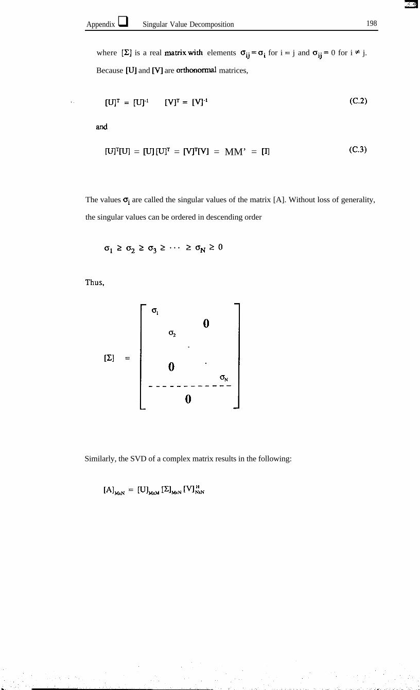
Appendix q Singular Value Decomposition 198
where [Z] is a real IX&X with elements Oij = bi for i = j and Oij = 0 for i # j.
Because yul and M are orbnormal matrices,
f . IU]= = m-1 [VI= = [vp
and
Wl=Wl = WlWl= = M=M = MM’ = El
(C.2)
(C-3)
The values ai are called the singular values of the matrix [A]. Without loss of generality,
the singular values can be ordered in descending order
Thus,
Similarly, the SVD of a complex matrix results in the following:

Appendix m Singular Value Decomposition 199
where [V],H, is the complex conjugate transpose of [VI and W] and [VI are unitary
matrices, i.e.,
MHM = MMH = l-4
and
pU]H = WI-1 MH = M-1
The singular values are the non-negative square roots of the eigenvalues of the matrix
INTEAl, if [Al is real, and of [AIHIA], if [A] is complex. Because [AITIA] is symmetric
and [AIHIA] is Hermitian, the eigenvalues are always real and non-negative [49] and,
therefore, singular values are always real and non-negative.
For simplicity, [A] will be assumed to be real from now on. Usually, the SVD
computation is performed in two stages: first, a reduction of [A] to a tridiagonal form
using the Householder transformation [49] and second, a reduction of the superdiagonal
elements to a negligible size, using the QR algorithm [49], resulting in a diagonal foxm.
h ,.. , _ _. ‘,i. ‘_ , L ,.

Appendix q Singular Value &composition 200
C.2 RANK OF A MATRIX
In some applications it is necessary to determine the rank of a matrix, particularly to
determine if the matrix is of less than full rank. The rank of [A] is the largest number of
columns (or rows) of [A] which constitute a linearly independent set. An MxN matrix
with IvPN is said to be of full rank if its rank equals N, but rank-deficient if its rank is
less than N.
To calculate the rank of a matrix, an algorithm such as Gaussian elimination may be
applied and the rank decided from the final reduced form. In practice, the situation is not
so simple. In the first place, the elements of a matrix are seldom given exactly and, even
if the original matrix is rank-deficient, it is unlikely that its approximation will also be.
Thus, instead of asking if the given matrix is rank-deficient, we must ask if it is nearly
rank-deficient. In the second place, the transformations of, say, Gaussian elimination
may take a matrix which is very nearly deficient in rank and turn it into one which is
clearly of full rank. Finally, it is not always easy to recognise when even a triangular
matrix, which is the end product of Gaussian elimination, is nearly deficient in rank.
The relationship between the SVD and the rank of a matrix is that the value of the rank is
equal to the number of non-zero singular values. The advantage of using the SVD to
calculate the rank is that if r rows of an NxN matrix are not totally linearly dependent, we
shall obtain a small value for ~~_r+~, instead of zero, and we have only to compare this
small value with other singular values. If we establish a criterion for the rejection and
acceptance of small singular values, we shall have ananswer concerning thevalue of the
rank. This criterion may depend on the accuracy of the expected results and, in practice,
may be difficult to establish. A reasonable solution is to calculate the consecutive ratios of
ON-1the singular values, :, O<, , . . -.ON
Representing the ratios graphically, the first peak
will indicate the value of the rank. For instance, if the rank of a matrix is r, then or,, will

Appendix q Singular Value Decomposition 201
be very small and the ratio 2 will be very high compared with %, which indicates theI
rank of the matrix.
C.3 THE LEAST-SQUARES PROBLEM
Very often, we have to solve least-squares problems. These happen when we have an
, over-specified set of equations with relation to the unknowns, i.e., we have more
information than we need to solve the problem. Once it has been established that a
coefficient matrix [A] is of full rank, the least-squares solution t0.a.n overdetermined set
of linear equations
can be obtained from
(x] = [Al;xM @I
where M > N, and [A&& is the Moore-Penrose genera&d inverse, ([A]‘[A])-‘[A]‘.
The generalised inverse [A]‘can easily be computed efficiently by using the SVD. From
equation (C.l), we obtain
[Al;, = [VI Gx, PI 1;=M WI ,‘,,
Substituting equation (C.3) into equation (C.4) leads to
[Al’ = WI El’ WIT
(C.4)

Appendix q Singular Value Decomposition 202
where [Cl’ is given by
I-1
01
[Cl’ =
Each element of [Zj’ can be easily calculated as
N6 = c ‘iklik
k=l
where vik and ujk are the corresponding elements of Iv] and [VJ.

Appendix m Dynamic Characteristics of Push Rod 203
APPENDIX D
DYNAMIC CHARACTERISTICS OF PUSH ROD
When modal testing is performed using a continuous excitation signal, such as random or
sinusoidal, it is necessary to use an exciter connected via a push rod which should have
high axial stiffness for transmission of axial force but low lateral or bending stiffness to
allow little moment transfer. In order for the push rod not to contaminate test results, the
natural frequencies of the push rod should lie well outside the test frequency range.
Dimensions and material properties of push rods which were used for the experiment in
Chapter 5 are shown in Table D.l.
Table D. 1 Dimensions and Material Pronerties of Push rods
t I I I 1 1
Long push rodShort push rod
d1.5 mm1.5 mm
L67.0 mm13.0 mm
E P2.07 ~10” N/m* 7850 kg/ma2.07 x1Otr N/m2 7850 kg/n+
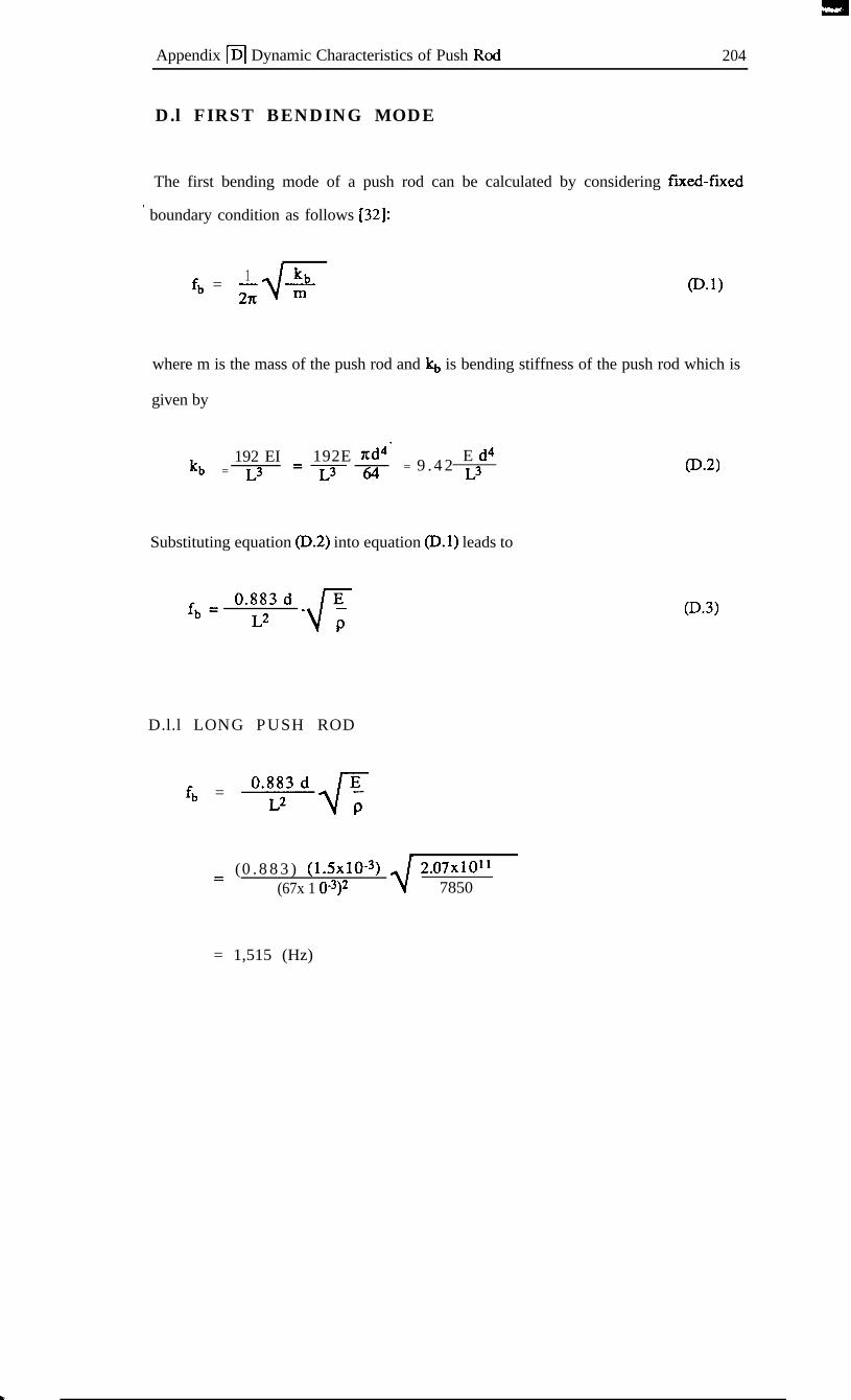
Appendix IDI Dynamic Characteristics of Push Red 204
D.l FIRST BENDING MODE
The first bending mode of a push rod can be calculated by considering fixed-futed
’ boundary condition as follows [32]:
fb = 1-II
kb2K m
@.l)
where m is the mass of the push rod and kb is bending stiffness of the push rod which is
given by
192 EIkb = ~3
192E xd4‘ E d4=y3- (jLj = 9.42 L3
Substituting equation (D-2) into equation (D.1) leads to
D.l.l LONG PUSH ROD
fb =
= (0.883) (1.5~10-~) 2.07~10”(67x 1 O-3)2 7850
= 1,515 (Hz)
@.a
P-3)

Appendix q Dynamic Characteristics of Push Rod 205
D.1.2 SHORT PUSH ROD
fb = (0.883) (1.5~10-~)(13x10-3)2
= 40,244 (Hz)
/ D.2 AXIAL MODE
In this case, the push rod assembly acts as a spring loaded by the mass of an exciter
armature. Thus,
@.49
where rq,, is the mass of the exciter mature and k, is the axial stiffness of the push rod
which is given by
D.2.2 LONG PUSH ROD
k, =(x/4) (1.5x1O-3)2(2.O7xlO11)
(67~10-~)
= 5.460 x 10⁶ (N/m)
05)
c

Appendix q Dynamic Characteristics of Push Rod 206
f, = $ 5.460 x 1060.02
= 2,630 (Hz)
D.2.2 SHORT PUSH ROD
k, = (X/4) (1.~x10-3)2(2.07X10’1)
(13x10-3)
= 2.815x lo7 (N/m)
2.815~10~0.02
= 5,917 (Hz)

Appendix m GENFRF User’s Guide 207
APPENDIX E
GENFRF USER’S GUIDE
E.l OVERVIEW
GENFRF is a FORTRAN program designed to run on an IBM PC-AT or PS2.
generate frequency response functions (FRFs) which have various measurement
such as:
1) mass loading effects of force transducer and accelerometer,
2) error by shaker/structure interaction;
3) input and output random noise;
4) signal processing error (leakage)
A flowchart of the program is given in Fig.E.l.
It can
errors
Generated FRFs can be directly used as input files of MODENT [37] for modal
analysis.

Appendix kl GENFRF User’s Guide
4ssemble to make global mass and stiffness matrices Eigenvdue solutionCALL,ELMKFl&GLOBAL
[AlA WA
and frequency range from data iYeIt
Introduce mismodelled regionsCALLdExMK
N
Read excitation point and response pointshm data file
It
I
Mass loading effect of force trasnsducerCALLMIDADF I
Mass loading effect of accelerometerCALLMILXDA A3
Fig.E. 1 (a) Flowchart of FRF Generation Program

Appendix q GENFRF User’s Guide 209
Shaker/structure interactionCALLFRFCAL&INTA~
Calculate noise-free FRFs
CALLFRFCAL
Store output in* TR****.FFW
Calculate auto ancj cross spectra of signals and noise autospectraand add noises to signals
Choose window functionCALLdWlNDOW
Calculate FRF & coherence
Calculate random errors of FRF & coherence
Store output inDB****.FRF
Move to next point
Fig.E. 1 (b) Flowchart of FRF Generation Program

Appendix q GENFRF User’s Guide 210
1QRead response point and excitation points
fi-omdatafile
I Mass loading effect of accelerometerCAILMLOADA I
t1 Hammer/strucm interaction
Calculate auto and cross spectra of signals and noise autospectraand add noises to signals
I
t
Calculate FRF & coherence
I Calculate random errors of FRF & coherent e(
Move to next point
Fig.E. 1 (c) Flowchart of FRF Generation Program
c

Appendix q GENFRF User’s Guide 211
E.2 INPUT FILE
To run the program, an input file GENFRF.DAT is necessary. Its format is @en in
Table E. 1.
Table E. 1 Format of GENFRF.DAT
RecordV a r i a b l e Name
3 IFTYPE INT
FRF Type (1 =Receptance, 2=Mobility, 3=Inertance)
5 AMS, FTMS, EXMS REAL
Masses of accelerometer, force transducer, mature (kg)
7 GMM, GNN, NAV REAL,REAL,I.NT
Input noise level, Output noise level, No of average
9 FST, FED REAL
S&g freq (Hz), Ending freq (Hz)
11 ICOH INT
0 = No coherence data, 1 = Coherence data available
13 IEX INT
15
17
19
Global excitation coordinate number
IRS1,1RS2....IRS,,
n Global response coordinate numbers
TITLE
First two characters of output file names
HEAD
Title for FRFs
INT
CHAR*2
CHAR*80
L.,. . :

Appendix @ GENFRF User’s Guide 212
1) Other records are only used for descriptions of following variables.
2) All data to be read in FORTRAN77 free format using the appropriate variable type
except TITLE (Record 17).
E.3 RUNNING GENFRF
1) When you see C:>, change to subdirectory WAG\ by typing
CD NAG
2) Run GENFRF by typing
GENFRF
3) After several messages, you will be asked:
IS SHAKER USED? ( YES = 0 , NO = 1 )
Type 0 for shaker excitation (Hammer excitation is not available, if type 1, the
program will be terminated.)
4) After a while, the computer will give a message
** CALCULATING FREQUENCY RESPONSE FUNCTIONS **
followed by calculated FRF file names.
E.4 GENFRF OUTPUT FILES
The output files of GENFRF are as follows:
1) Exact modal data ANAL.DAT
2) n (no of measurement coordinates) error-free FRF data files (TRNlN2.FRF) and
n noisy FRF data files (DBNlN2.FRF) where
N 1; Response coordinate (2 digit)
N2; Excitation coordinate (2 digit)

Appendix m GENFRF User’s Guide 213
Data format of these files is given in Appendix C of MODENT Reference Marx.&
3) Combined Response Data file (BEAMSRD). This data file contains the names of
individual FRF files to be analysed globally. Data format is given in Appendix C of
MODENT Reference Manual.
ES MODIFYING PROGRAM
GENFRF program uses one of NAG routines, F02AEF, for eigenvalue solution which
is stored in subdirectory NAG. If you want to modify the program
1) Change to subdirectory WAGj and modify GENFRF.FOR.
2) After editing, type
FL /AH /Opx /FPc genfrf . for /link wlms3+wlms4+wlms5+wlms6+wlms7
for compiling and linking because NAG routines were compiled with the options.
3) Type
GENFRF
to run the modified program.

Appendix q GENFRF User’s Guide 214
E.6 COMPUTER PROGRAM
c*******************************************************************c
c*******************************************************************c
c***** *****c
c***** PROGRAM FOR SIMULATING EXPERIMENTAL DATA *****cc***** *****cC****************************************************~**************CC***********************************************~*******************C
PROGRAM SIMULATIONc*******************************************************************cc***** *****cc***** FREE-FREE BEAM STRUCTURE *****cc***** *****cc*******************************************************************c
PARAMETER(NEL=20,N=42,M=l O,NFP=40 1 ,NF2=801)c*******************************************************************c
C***** VARIABLES *****c
C***** N ; NO-OF DOF OF SYSTEM *****c
C***** M ; NO.OF MEASURED MODES *****c
C***** NFP ; NO.OF FREQUENCY POINTS *****c
c***** NF2 ; @m-1)*2+1 *****c
c********************************************************************c
DOUBLE PRECISION EVAL,EVEC,DUMM,DUMK,DL,EDIMENSION DEM(4,4),DEK(4,4)DIMENSION DL(N),E(N)DIMENSION DUMM(N,N),DUMK(N,N)DIMENSION FREQ( lO),COH(NFP)DIMENSION GFF(NF2),GXX(NF2)CHARACTER TITLE*2,FLNM*lO,EX*2,RSP*2CHAIbJCIER HEAD*80COMPLEX CFRF,GXF(NF2)COMMON /CB l/FMF(N,N),FKF(N,N)COMMON /CB2/DMM(N,N)COMMON /CB3/DM(N,N),DK(N,N)COMMON /CB4/EVAL(N),EVEC(N,N)COMMON /CBS/CFRF(NF2),FSM(NF2)
C

Appendix @ GENFRF User’s Guide 215
C**** ASSEMBLE GLOBAL MASS AND STIFFNESS MATRICESc
C
20C
30c
-(*,*IWRlTE(*,*)‘** ASSEMBLING MASS AND STIFFNESS MATRICES **’
mlTlx*,*)
DO 20 I=l,NDO 20 J=l,NDM(I,J)=O.DK(I,J)=O.CONTINUE
DO30K= 1;NELCALL ELMKFl (DEM,DEK,K)DO 30 I=l,NDO 30 J=l,NDK(I,J)=DK(I,J)+FKF(I,J)DM(I,J)=DM(I,J)+FMF(I,J)CONTINUE
C**** CALCULATE ANALYTICAL NATURAL FREQUENCIES &C**** MODE SHAPESC
DO 40 I=l,NDO 40 J=l,NDUMM(I,J)=DM(T,J)DUMK(I,J)=DK(I,J)
40 mNTINuEC
IFAIL=OC
CALL FO2AEF@UMK,N,DUMM,N,N,EVAL,EVEC,N,DL,E,IFAIL)CC?*** INTRODUCE MISMODELLED REGIONSC
CALLEXMKCC**** READ INPUT FILE (FRF+ IS INERTAWE)

Appendix q GENFRF User’s Guide 216
C
C
C
C
C
C
C
IC
C
OPEN(9,FILE=‘LEAK2.DAT,STATUS=‘OLD’)
I=w9,*)-(9**)RE%D(S,*) IFTYPER=w9,*)READ(9,*) AM$FrM$EXMSI=w9,*)READ(9,*) GMM,GNN,NAV=(9,*)READ(9,*) FST,FEDI=w9,*)READ(9,*) ICOHI=w9,*>I=w9,*> IEXI=w9**>READ(9,*) IRS=AD(9,*)READ(9,9950) TITLEI=w9,*)READ(9,9960) HEADCLOSE(g)
IF(IEX.LT. 10) THEN
wFuTE(Ex,9cm) IEX
ELSE
wRITE(Ex,9 loo) IEX
ENDIF
FR=(FED-FST)/(NFP-1)
C**** CALCULATE EXACI. NATURAL FREQUENCIES & MODE SHAPESC

Appendix q GENFRF User’s Guide 1 217
DO 70 I=l,NDO 70 J=l,NDUMM(I,J)=DM(I,J)DUMK(I,J)=DK(I,J)
7 0 C O N T I N U EC
IFAIL=C
CALL Fo2AEF@UMK,NPUMM~~~V~,EVEC,NPL,E,IFAIL)CC**** MASS LOADING E%ECIS OF FORCE TRANSDUCERC
CALLMLOADF(IEX,FI’MS)C
/ CC**** OPEN COMBINED RESPONSE DATA FILEC
C
C
C
C
C
C
1 cCC
C
IDuM=o
mIJw*,*)WRI’TE(*,*) ‘*** CALC’ULATING FRF ***’
mm(*,*)
IF(IRS.LT. 10) THEN
WRITE(RSP,9000) IRS
ELSE
WRITE(RSP,9 100) IRS
ENTXF
MASS LOADING EFFECTS OF ACCELEROMETER
CALLMLOA.DA(IRS~S)
C**** CALCULATE NATURAL FREQUENCIES & MODE SHAPES

Appendix q GENFRF User’s Guide 218
CDO 110 I=l,NDO 110 J=l,N
DUMW.&J)=DMW&J)DUMK(I,J)=DK(I,J)
110 CONTINUEC
IFAIL=C
CALL Fo2An;@U~NPUMM~~~V~,E~C~PL,E~~)CC**** SHAKER/STRUCIURE INTERACYIONC
CALL FRFCAL(FST,FED,IEX,IEX)C
CALLINTACT(EXMS)CC DEFINE EXCITATION NODE(lEN) AND DIRECl-ION(lED)C
IEN=lIED=
CC CALCULATE RESPONSE NODE(IRN) AND DIRECTION(IRD)C
IRN=5IRD=2
CC**** CALCULATE NOISE-FREE FRF H(IRS,IEX)C
CALL FRFCAL(FST,FED,IEX,IRS)C
FLNM=‘TR’//RSP//EX/l.FRFC
OPEN (UNIT=lO,FILE=FLNM,STATUS=‘UNKNOWN’)C
wRtTE(10,9960) HEADWRITE(lO,*) IFIYPEWRITE( 10,94OO) NFP,FST,FR
-_

Appendix q GENFRF User’s Guide 219
wRITE( lo,*) ‘0’WRITE( lo,*) IEN,IED,IRN,IRD,IDUMwRITE(lo,*) ’ 00000
wRlTE( lo,*) IEX,IRSwRITE( 10,950O) pRF(I*2- l),I=l &FP)
CFIN=FST
CDO 111 J=l,(NFP+9)/10Do 112 I=l,lOFREQ(I)=FIN+(I-l)*FR
112 CONTINUEWRITE(10,9700) (FREQ(I),I=l,lO)FIN=FREQ( 1 O)+FR
1 1 1 mNTINUECC**** CALCULATE AU-IO AND CROSS SPECI’RACC CALCULATE NOISE-FREE AUTO AND CROSS SPECTRAC
GPP=l.OC
Do 125 I=l,NF2GFF(I)=FSM(I)*GPPGXX(I)=(REAL(CFRF(I))**2+AIMAG(CFRF(I))**2)*GFF(I)GXF(I)=GXX(I)/CFRF(I)
125 CONTINUECC ADD NOISE To SPECTRAC
Do 130 I=l,NF2GFF(I)=GFF(I)+GMMGXX(I)=GXX(I)ffiNN
1 3 0 CmmNuECC**** LEAKAGE EFFECTC
Do 140 I=l,NF2

Appendix m GENFRF User’s Guide 220
140c
C
150C
160C
CI
170C
C
CFRF(I)=CMPLX(GFF(I),O.)CONTINUE
CALLLEAK(CFRFJ;R)
Do 150 I=l,NFPGFF(I*2-l)=REAL(CFRF(I*2-1))CONTINUE
DO 160 I=l,NF2CFRF(I)=CMPLX(GXX(I),O.)CONTINUE
CALL LEAK(CFRF,FR)
DO 170 I=l,NFPGXX(I*2- l)=REAL(CFRF(I*2-1))CONTINUE
CALL LEAK(GXF,FR)
C**** CALCULATE FREQENCY RESPONSE FUNCTION H2C
DO 180 I=l,NFPCFRF(I*2-l)=GXX(I*2-l)/GXF(I*2-1)
180 CONTINUECC**** CALCULATE COHERENCE FUNCI’IONC
DO 190 I=l,NFPCOH(I)=CABS(GXF(I*2-1))**2/(GFF(I*2-1)*GXX(I*2-1))IF(COH(I).GT. 1 .O) COH(I)=l .O
I 190 CONTINuECC**** CALCULATE RANDOM ERROR OF H2C
DO 200 I=l,NFPERH=SQRT(( l.-COH(I))/(COH(I)*2. *NAV))

Appendix q GENFRF User’s Guide 221
IR1=987*I*IRN+lIR2=789*I*IRN+lRAND1=2.0*(RAN3(IRl)-0.5)RAND2=2.0*(RAN3(IR2)-0.5)REH =( 1 .otERH*RAN-D l)*REAL(CFRF(I*2- 1))AIMH=( l.O+ERH*RAND2)*AIMAG(CFRF(I*2- 1))CFRF(I*2- l)=CyPLx@EH&MH)
2 0 0 CONTINUECc**** CALCULATE RANDOM ERROR OF COHERENCEC
C
210C
C
220C
C
C
C
IF(NAV.EQ. 1) THEN
Do 210 I=l,NFPCOH(I)=l.OCmTINUE
ELSE
Do 220 I=l,NFPERG=(SQRT(2.)*(1.-COH(I)))/ISQRT(COH(I)*NAV)IRR=897*I*IRN+lRAND3=2.0*(RAN3(IRR)-0.5)CoH(I)=( 1 .O+ERG*RAND3)*COH(I)CoNTINUE
ENDIF
FLNM=TITLE//RSP//EX/r.FRF
OPEN (UNIT=lO,FILE=FLNM,STATUS=‘UNKNOWN’)
WRITE( 10,996O) HEADWRITE(lO,*) IFIYPEWRITE( 10,940O) NFP,FST,FRWRITE(lO,*) ICOHWRITE( lo,*) IEN,IED,IRN,IRD,IDUMWRITE(lo,*) ’ 00000
t. .,x I.

Appendix q GENFRF User’s Guide 222
C
C
310
300C
C
91009200930094009500960097009800
99509960C
C
WRITE( lo,*) IEX,IRSWRxTE( 10,950O) (CFRF(I*2- l),I=l ,NFP)WRITE( 10,960O) (COH(I),I=l ,NFP)
FIN=FST
DO 300 J=l,(NFP+9)/10DO 310 I=l,lOFREQ(I)=FIN+(I- l)*FRCONTINUEWRlTE(10,9700) (FREQo~=l,lO)FIN=FREQ( 1 O)+FRCONTINuE
CLOSE( 10)
FORMAT( lHO,I 1)FORMAT(l2)FORMAT(2X,I3,Fl5.2)FORMAT(F7.1,7X,2G 10.3)FORMAT(7X,I5,2F10.3)FORMAT(8E10.3)FORMAT(lX,lOF7.3)FORMAT(lX,lOF7.1)FORMAT(2E15.7)FORMAT( 1015)FORMAT( lX,A2)FORMAT(A70)
STOP

Appendix @ GENFRF User’s Guide 223
c*************************************************~~****************c
c***** *****c
c***** SUBROUTINES *****cc***** *****cc*******************************************************************c
Cc*******************************************************************cc***** SUBROUTINE EXMK *****cc*******************************************************************c
SUBROUTINE EXMKPARAMETER(N=42)DIMENSION DEM(4,4),DEK(4,4)COMMON /CB l/FMF(N,N),FKF(N,N)COMMON /CB3/DM(N,N),DK(N,N)
CC**** MASS MODIFICATIONSC
CALL ELMKFl@EM,DEK,l)C
DO 10 I=l,NDO 10 J=l,NDM(I,J)=DM(I,J)+l .O*FMF(I,J)
10 CONTINUEC
CALL ELMKFl(DEM,DEK,2)C
DO 20 I=l,NDO 20 J=l,NDM(I,J)=DM(I,J)+l .O*FMF(I,J)
20 CONTINuECC**** STIFFNESS MODIFICATIONSC
CALLELMKFl@EM,DEK,ll)C
DO 110 I=l,NDO 110 J=l,N
C DMK(I,J)=DK(I,J)+l .O*FKF(I,J)

Appendix q GENFRF Useis Guide 224
110C
C
C
120C
C
4 C
DK(I,J)=DK(I,J)+l .O*FKF(IJ)
CONTINUE
CALLELMKFl@EM,DEK,12)
DO 120 I=l,NDO 120 J=l,NDMK(I,J)=DMK(I,J)+l .O*FKF(I,J)DK(I,J)=DK(I,J)+l .O*FKF(I,J)
CONTINUE
RETURN
c**********************************************************~********c
c***** SUBROUTINE INTACI’ *****c
C***************************************************~****************C
SUBROUTINE INTACI’(EXMS)PARAMETER(NF2=801)COMPLEXCFRFCOMMON /CBXFRF(NF2),FSM(NF2)
CC**** SHAKER/STRUCI’URE INTERACl-IONCC FORCE SPECTRUM MODIFICATION FACI-ORC
C Gff(I)*pp(I)/((l+EXMS*H(I))*(l+EXMS*H*(I)))C
DO 10 I=l,NF2HMS=REAL(CFRF(I))**2+AIMAG(CFRF(I))**2FSM(I)=l./(l.+EXMS**2*HMS+2.*EXMS*REALQRF(I)))
10 mNTINuEC
RETURN
CC

Appendix q GENFRF User’s Guide 225
c********************************************************#**********cc***** SUBROUTINE MLOADF *****cC****************************************~***************************C
SUBROUTINE MLxIADF(TRS,A.MS)PARfamzR(N42)
COMMON /CB3/DM(N,N)PK(N,N)CC**** MASS LOADING EFFEClT OF FORCE TRANSDUCERC
DM(IRS,lRS) = DM(IRS,IRS)+AMS
CRETURN
CI c*******************************************************************c
c***** SUBROUTlNE WADA *****c
c*******************************************************************c
SUBROUTINE MLOADA(IRS,AMS)PARAMETER(N42)COMMON /CB2/DMM(N,N)COMMON /CB3/DM(N,N),DK(-N,N)DO 10 I=l,NDO 10 J=l,NDMM(I,J)=DM(I,J)
1 0 C O N T I N U ECC**** MASS LOADING EFFE(JTS OF ACCELEROMETERC
DMM(IRS,IRS) = DM(IRS ,IRS)+AMS
CRETURN
C
*. ,

Appendix q GENFRF User’s Guide 226
c****************************************************************~**c
c***** SUBROUTINE FRFCAL *****cC*********************************************~*********************C
SUBROUTINE FRFCAL(-FST,FED,IEX,IRS)PARAMETER(N=42,NF2=801)DOUBLE PRECISION EVAL,EVECCOMPLExCFRFpNTCoMMON/CIWEVALoWEC(N,N)COMMON /CBS/CFRF(NF2),FSM(NF2)
CC**** FRF(INERTANCE) CALCULATIONC
FRSL=(FED-FST)/(NF2- 1)C
DO 10 IFQ=l,NF2FREQ=FST+(IFQ- l)*FRSLSOMGA=(2.*3.1415927*FREQ)**2CFRF(IFQ)=(O.,O.)
CDO 20 IMD=l,N
CC DEFINE LOSS FAtXORS (DAMPING IS PROPORTIONAL)C
ETA=lOO.JEVAL@MD)+O.O05C
DRE=SOMGA-EVAL(IMD)DIM=EI’A*EVAL(IMD)DNT=CMPLX@RE,DIM)CFRF(IFQ)-XFRF(IFQ)+EVEC(IRS,IMD)*EVEC(IEX,IMD)*SOMGA/DNT
C20 CONTINUEC10 CONTINUEC
IF(CABS(CFRF( l)).EQ.O.) THENC
RECl= (2.*REAL(CFRF(2))- REAL(CFRF(3))) *REAL(CFRF(2))AICl=(2.*AIMAG(CFRF(2))-AIMAG(CFRF(3)))*AIMAG(CFRF(2))

Appendix q GENFRF User’s Guide 227
CFRF(l)=cMPLx(REcl~Icl)C
ENDIFC
RETURN
Cc*******************************************************************c
C**** FUNCTION RAN3 ****cc*******************************************************************c
FUNCI’ION RAN3(IDUM)IMPLICIT REAL*4(M)PARAMETER (MBIG=WKWO.,MSEED=1618033.,MZ=O.,FAC=2.5E-7)DIMENSION MA(55)
CDATA IFF/o/
CIF(IDUM.LT.O.OR.IFF.EQ.0) THEN
CIFF= 1MJ=MSEED-IABS(IDUM)MJ=MOD(MJ,MBIG)MA(55)=MJMK=l
CDO 11 1=1,54II=MOD(21*1,55)MA@)=MKMK=MJ-MKIF(MK.LT.MZ) MK=MK+MBIGMJ=MA@I)
11 CONTINUE! C
DO 13 K=1,4DO 12 1=1,55MA(I)=MA(I)-MA( l+MOD(I+30,55))IF(MA(I).LT.MZ)MA(I)=MAO+MBIG
12 CcmTrNUE
L ,._, ., , _, , .- ir, . ,_, . _., .,. .: ”

Appendix q GENFRF User’s Guide 228
1 3 C O N T I N U EC
INExT=INExTP=3 1IDUM=l
CENDIF
CrNExT=INJzT+lIF(INEXT.EQ.56) IN-EXT=lmJExTP=INExTP+lIF(INEXTP.EQ.56) JNEXTP=lMJ=MA(INExT)-MA(INEm-P)IF(MJ.LT.MZ) MJ=MJ+MEHGMA(INExT)=MJ .
RAN3=MJ*FACC
RETURN
CCc*******************************************************************cc***** SUBROUTTNE.EMASS *****cc*********************************************************************c
SUJ3ROUTINE EMASS@EM,ICLASS)DIMENSION DEM(4.4)
CDENS=7800.
CIF(ICIASS .EQ. 1) THENEIiO.075AREA=S.OE-4GOT010
CELSEIF(ICLASS .EQ. 2) THENEL=SQRT( 1.93)/6.AREA=l.2SE-4
GOT0 10

Appendix q GENFRF User’s Guide 229
CELSEIF(ICLASS .EQ. 3) THENELF0.175AREA=lSE-4GOT010
CENDIF
C1 0 CONTINUEC
FAC=DENS*AREW*W420.CC**** UPPER TRIANGULAR ELEMENTS OF ELEMENT MASS MATRIXC
DEM(l,l)=156.DEM( 1,2)=22.*ELDEM( 1,3)=54.DEM(1,4)=-13.*ELDEM(2,2)=4.*EL**2DEM(2,3)=13.*ELDEM(2,4)=-3.*EL**2DEM(3,3)=156.DEM(3,4)=-22.*ELDEM(4,4)=4.*EL**2
CDO 15 1=1,4DO 15 J=I,4DEM(I,J)=FAC*DEM(I,J)
15 CONTINUECc**** mom MASS MAW **************c
CDO 20 1=2,4DO 20 J=l,I-1DEM(I,J)=DEM(J,I)
20 CONTINUEC
RETURN
.

Appendix m GENFRF User’s Guide 230
c***** SUBROUTINE ESTIFF *****cc*******************************************************************c
C
I
C
i/
C
C
C
10C
C
SUBROUTINE ESTIFF@EK,ICLASS)DIMENSION DEK(4,4)E=209.E9
lF(ICLASS EQ. 1) THENEL=O.O75AMkOA1667E-8GOT0 10
ELSEIF(ICLASS .EQ. 2) THENEL=SQRT( 1.93)/6.AMI=l.O417E-11GOT010
ELSEIF(ICLASS .EQ. 3) THENEL=O. 175AMI=1.25E-11GOT010
ENDIF
CONTINUE
FAC2=E*AMI/EL**3
c**** SJp-FNFSS mm ********c
CD&(l,l)=FAC2*12.DEK( 1,2)=FAC2*6.*ELDEK( 1,3)=-DEK( 1,l)DEK( 1,4)=DEK( 1,2)DEK(2,2)=FAC2*4.*EL**2DEK(2,3)=-DEK( 1,2)

Appendix q GENFRF User’s Guide 230
Cc*************************************************~******************~c***** SUBROUTINE ESTIFF *****ec*******************************************************************~
C
C
C
C
C10C
C
SUBROUTINE ESTIFF@EK,ICLASS)DIMENSION DEK(4,4)E=209.E9
lF(ICLASS .EQ. 1) THENEL=O.075AMI=O.41667E-8GOT010
ELSEIF(ICLASS .EQ. 2) THENEL=SQRT( 1.93)/6.AMI=l.O417E-11GOT010
ELSEIF(ICLASS .EQ. 3) THENEM.175AM_I=1.25E-11GOT010
ENDIF
CONTINUE
FAC2=E*AMI/EL**3
c**** smss mm ********c
CDEK(l,l)=FAC2*12.DEK( 1,2)=FAC2*6.*ELDEK( 1,3)=-DEK( 1,l)DEK( 1,4)=DEK( 1,2)DEK(2,2)=FAC2*4.*EL**2DEK(2,3)=-DEK( 1,2)

Appendix q GENFRF User’s Guide 231
DEK(2,4)=DEK(2,2)/2.DEK(3,3)=DEK( 1 ,l)DEK(3,4)=DEK(2,3)DEK(4,4)=DEK(2,2)
c
DO 20 1=2,4DO 20 J=l,I-1DEK(I,J)=DEK(J,I)
20 CONTINUERETURN
Cc*******************************************************************cc***** SUBROUTINE ELMKFl *****cr***************************************************~***************CL
C
10C
C
C
C
C
C
SUBROUTINE ELMKFl@EM,DEK,K)PARAME’IER(N=42)DIMENSION DEM(4,4),DEK(4,4)COMMON /CB l/FMF(N,N),FKF(N,N)
DO 10 I=l,NDO 10 J=l,NFMF(I,J)=O.FKF(I,J)=O.CONTINUE
IF(K.GE.l .AND. K.LE.21) THEN
CALLEMASS(DEM,l)CALL ESTIFF(DEK, 1)
ELSE
WRIT&*,*) ‘*** ASSEMBLING ERROR !! ***’STOP
ENDlF
_.’ ..,I .._. _I ..‘F-r .._ ,,.. _. < ,... I. . . ~
.-

Appendix m GENFRF User’s Guide 232
C
20C
C
C
C
C
IF(K.GE.1 .AND. K.LE.21) THEN
DO 20 1=1,4DO 20 J=1,4
FMF((K-1)*2+1&1)*2+J)=DEM(I,J)FKF((K- 1)*2+I,(K- 1)*2+J-)=DEK(I,J)
cxmTmuE
ELSE
WRITE(*,*) ‘*** ASSEMBLING ERROR !! ***’
STOP
c*******************************************************************c
c***** SUBROUTINE GLOBAL *****c
r*******************************************************************cL
SUBROUTINE GLOBAL(NI,NJ,DEM,DEK)PARAMETER(N=42)DIMENSION DEM(4,4),DEK(4,4)COMMON /CB l/FMF(N,N),FKF(N,N)
C
20
3010CC
DO 10 I=12DO20 J=1,2FMF((NI- 1)*2+I,(NI- 1)*2+J)=DEM(I,J)FKF((NI-1)*2+I,(NI-1)*2+J)=DEK(I,J)CONTINUEDO 30 J=3,4FMF((NI-1)*2+I,(NJ_2)*2+J)=DEM(I,J)FIF((NI-1)*2+I,(NJ_2)*2+J)=DEK(I,J)CONTINUECcwTINUE
L

Appendix q GENFRF User’s Guide 233
DO 40 1=3,4DO 50 J=1,2FMF((NJ-2)*2+I,(NI-1)*2+J)=DEM(I,J)FKF((NJ-2)*2+I,(NI-1)*2+J)=DEK(I,J)
50 CONTINUEDO 60 J=3,4FMF((NJ-2)*2+I,(NJ_2)*2+J)=DEM(I,J)FKF((NJ-2)*2+I,(NJ_2)*2+J)=DEK(I,J)
%O CONTINUE40 CONlTNm.C
RETURN
CC******************************************************~************Cc***** SUBROUTINE LEAK *****c
C*********************************************~*********************C
C
C
C
C
C
1234
C
C
SUBROUTINE LEAK(GXYfl)PARAMETER(NF2=801)COMPLEX GXY(NF2),GD(NF2)
Do 10 I=l,NF2,2
IF(I.LE.5 .OR. I.GE.NFZ5) THEN
GD(I)=GXY(I)*3./FR
ELSE
GD(I)=2.*GHAN(FR,2S*FR)*(GXY(I_S)+GXY(I+S))+2.*GHAN(FR,l.5*FR)*(GXY(I-3)+GXY(I+3))+GHAN(FR,FR)*(GXY&2)ffiXY(I+2))+2.*GHAN(FR,O.5*FR)*(GXY(I-l)+GXY(I+l))+GHAN(FR,O.)*GXY(I)
ENDIF
GD(I)=GD(I)*FW3.

CC*****************************************~~************************C
c***** FUNClJON GHAN *****cr*******************************************~*******************~****CL
C
C
C
C
C
C
FUNCTION GHAN(FR,FX)
IF(FX.EQ.0) T H E N .
GHAN=2./(3.*FR)
ELSEIF(FX.EQ.FR) THEN
GHAN=1./(6.*FR)
ELSE
CST=FR/3.1415927**2T1=2./(3.*FX**2)T2=1./6.*(1./(FX+FR)**2+1./(F=W**2)T3=1./(FR**2-FX**2)X=(3.1415927*FX)/FRGHAN=CST*(Tl+T2+T3)*SIN(X)**2
C
C
C
ENDIF
RETURN
Appendix q GENFRF Usefs Guide 234
1 0 C O N T I N U EC
Do 20 I=l,NF2GXW)=GW)
2 0 cmam-uEC
RETURN
*

Appendix q GENFRF User’s Guide 235
E.7 DATA FILE
FREE-FREE BEAM DATA (PROP. STRUCIVRAL DAMPING)FRF TYPE (INERTANCE=3)3
MASSES (ACCELEROMETER, FORCE TRANSDUCER & SHAKER)0.02 0.01 0.02
NOISE SPECTRA LEVELS (INPUT & OUTPUT) AND NO. OF AVERAGEl.OE-2 l.OE-3 100
STARTING FREQ. AND END FREQ.0. 800.
COHERENCE FLAG1
EXCITATION COORDINATE
RESPONSE COORDINATES1 5 9 13 17 21 25 29
4133 37

Appendix m Bendent Method 236
APPENDIX F
BENDENT METHOD
Even though the Inverse method for SDOF identification of a FRF has some advantages
over the Circle-fit method as discussed in Chapter 5, the Inverse method. has some
drawbacks such that:
1) it is difficult to apply the Line-fit method to complex modes, and
2) the extraction of the residual effects of other modes is a pre-requsite for an accurate
analysis.
A new SDOF method, which is a modified version of the Inverse Method , has been
developed by Dobson [51]. This method retains many of the advantages of the Inverse
method and can calculate modal parameters of complex modes.
The receptance FRF near resonance can be express as
a(o) = Arco,* - co* + i qr Or*
+ Rr (Fl)
where A, and R, are complex. The effect of Rr can be eliminated by taking the difference
between two measured FRF data.
; .- , ~. -.^ , .-“G ._‘i_, _.. j _ ..,, .: ,.

Appendix q Bendent Method 237
I&t02-R2
a’(@ = a(o) - a(Q) and A(o) -a’(W
where R is a reference frequency. Then,
A(m) = (or2 - 612+ i lJr Or’) (CO,‘- f2’ + i Tjr 0,‘)A,
= Re (A) + Im (A)
(F2)
(F3)
where Re (A) = mR 61? + cR and Im (A) = mI 02 + CI
and mR=- a, (CO,’ - Q2) - br (rlr 6%‘)
I Ar 1’
np =b, (61, - n2) - a, (qr 6%‘)
I Ar 1’
A, = a,+ib,
The slopes of the real and imaginary components of A are linear functions of R2 such
that:
mR = n&‘+dR and
where the slopes and intercepts are:
nR =a,
I A, I2
dR = -aror‘- brqr or2I A, I2
nI = - brI A, I2
(F4)
Wa)
t-b)
WC)

Appendix m Bendent Method 238
dI = - a,rjr or2 + b,mr2I A, I2
This set of equations can be used to extract the modal properties. From equations @a)
and (F5c)
b,=-2%
where p = 2
From equations (F5b) and (F5d)
d1where q = -dR
From equations (F5a) and (F5b)
(-J&2 = - dR
nR(l-Pqr)and
a, = 0r2(Ptlrv1)dR(l+P2)
therefore b, can be calculated from equation (F6).
For real modes (b, = 0), p = nI = 0, therefore,
- dR(42 = -"R
033
039
0-3

Appendix q Bendent Method 239
The analysis is in two parts.
1) For the selected FRF data range one point is selected as the reference point R. All
possible values of A(o) are calculated using the reminder of the selected data. The best
straight line is then calculated for each of the real and imaginary parts of equation (F3)
to determine the values of mR and rq for that value of R. The process is repeated using
each of the data points in turn as a reference point, and a series of lots made, showing
the values for Re (A) and Im (A) against ~2.
2) The slopes of the best fit straight lines for each in part 1 are plotted against the
reference frequency R. The resulting two plots may either be analysed using a straight
line fit over the whole range or over the selected range.


References 241
REFERENCES
1. Ewins, D.J. and Imregun, M.
“State-of-the-Art Assessment of Structural Dynamic Response Analysis Methods
(DYNAS)“,
Shock and Vibration Bulletin, Vol. 56, Part 1, August 1986.
2 . Rodden, W.P.
“A Method for Deriving Jnfluence Coefficients from Ground Vibration Test”,
AIAA Journal, Vol. 5, No. 5, 1967, pp. 991-1000.
3. Berman, A. and Flannelly, W.G.
“Theory of Incomplete Models of Dynamic Structures”,
AIAA Journal, Vol. 9, No. 8, 1971, pp. 1481-1487.
4 . Baruch, M. and Bar-Itzhack, I.Y.
“Optimal Weighted Orthogonahzation of Measured Modes”,
AIAA Journal, Vol. 16, No. 4, 1978, pp. 346-351.
5. Baruch, M.
“Optimization Procedure to Correct Stiffness and Flexibility Ma&es Using
Vibration Data”,
AIAA Journal, Vol. 16, No. 11, 1978, pp. 1208-1210.
;. ,., ,i ., _., ‘ _ ._~_ .; ,, ~~_

References
6 . Berman, A.
“Comment on Optimal Weighted Orthogonalization of Measured Modes”,
AIAA Journal, Vol. 17, No. 8, 1979, pp. 927-928.
7 .
8 .
9 .
10.
11.
12.
Berman, A.
“Mass Matrix Correction Using an Incomplete Set of Measured Modes”,
AIAA Journal, Vol. 17, No. 10, 1979, pp. 1147-1148.
Berman, A. and Nagy, E.J.
“Impro&nent of a Large Analytical Model Using Test Data”,
AIAA Journal, Vol. 21, No. 8, 1983, pp. 1168-1173.
Wei, F.S.
“Stiffness Matrix Conztion from Incomplete Test Data”,
AIAA Journal, Vo1.18, No. 10, 1980, pp. 1274-1275.
Caesar, B.
“Update and Identification of Dynamic Xathematical Models”,
Proc. IMAC 4, 1986, pp. 394-401.
Lin, R.M. and Jung, H.
“Possibilities and Limitations of Analytical Model Improvement ---- A Review
Based on the GARTEUR Exercise”,
Internal Report No.90001, Dynamics Section, Imperial College, Feb. 1990.
To, W.M.
242
“Sensitivity Analysis of Mechanical Structures Using Experimental Data”,
Ph.D. Thesis, Dept. of Mech. Eng., Imperial College, 1990.
L ., .-

References 243
13. Ibrahim, S.R., Stravinidis, C., Fisette, E. and Brunner; 0.
“A Direct Two Response Response Approach for Updating Analytical Dynamic
Models of Structums with Emphasis on Uniqueness”,
Proc. IMAC 7.1989, pp. 340-346.
14. Collins, J. D., Hart, G. C., Hasselman, T. K. and Kennedy, B.
“Statistical Identification of Structure”,
AIAA Journal, Vol. 12, No. 2, 1974, pp. 185-190.
‘15 . Chen, J.C. and Garba, J.A.
“Analytical Model Improvement Using Modal Test Results”,
AIAA Journal, Vol. 18, No. 6, 1980, pp. 684-690.
16. Sidhu, J. and Ewins, D.J.
“Con-elation of Finite Element and Modal Test Studies of a Practical Structure”,
Proc. IMAC 2, 1984, pp. 756-762.
17.
18.
19 .
He, J.
“Identification of Structural Dynamics Characteristics”,
Ph.D. Thesis, Dept. of Mech. Eng., Imperial College, 1987.
Fisette, E., Stravinidis, C., and Ibrahim, S.R.
“Error Location and Updating of Analytical Dynamic Models Using a Force Balance
Method”,
Proc. IMAC 6, 1988, 1063-1070.
Zhang, Q., Lallement, G., Fillod, R., and Piranda, J.
“A Complete Procedure for the Adjustment of a Mathematical Model from the
Identified Complex Modes”,
Proc. IMAC $1987, pp. 1183-l 190.

References 244
20. Caesar, B.
‘Updating System Matrices Using Modal Test Data”,
Proc. IMAC $1987, pp. 453-459.
21. Lin, R.M.
22. Lieven, N.A?J. and Ewins, D. J.
“Expansion of Modal Data for Correlation”,
Proc. IMAC 8,1990, pp. 605609.
23. Gysin, H.
“Comparison of Expansion Methods for FE Modeling Error Localization”,
Proc. IMAC 8, 1990, pp. 195-204.
24. Guyan, R. J.
“Reduction of Stiffness and Mass Matrices”,
AIAA Journal, Vol. 3, No. 2, 1965, p. 380.
25. Urgueira, A. P. V.
“Couple Structure Analysis Using Incomplete Modes”,
Internal Report No.88012, Dynamics Section, Imperial College, 1988.
26. Lim, K.B., Junkins, J.L. and Wang, B.P.
“Re-examination of Eigenvector Derivatives”,
J. Guidance, Vol. 10, No. 6, 1987, pp. 581-587.
27. Allemang, R.J. and Brown, D.L.
‘A Correlation Coefficient for Modal Vector Analysis”,
Proc. IMAC 1. 1982. DD. 1 lo-1 16.
“Identification of the Dynamic Chamcuzistics of Nonlinear Structures”,
Ph.D. Thesis, Dept. of Mech. Eng., Imperial College, 1991.
c . ,#.

References 245
2 8 . Ewins, D.J. and Griffin, J.
“A State-of-the-Art Assessment of Mobility Measurement Techniques -
Results for the Mid-Range Structures (30 - 3,000 Hz)“,
Journal of Sound & Vibration, Vol. 78, Part 2’1981.
2 9 . Ewins, D.J.
“Modal Testing : Theory and Practice,,,
Research Studies Press, London, 1984.
3 0 . Broth, J.T.
‘Mechanical Vibration and Shock Measurements”, 2nd ed.,
Brtiel & Kjar, 1984.
3 1 . Mitchell, L.D. and Elliot, K.B.
“A Method for Designing Stingers for Use in Mobility Testing”,
Proc. JMAC 2, 1984, pp. 872-876.
32 .
3 3 .
3 4 .
3 5 .
Hieber, G.M.
“Non-Toxic Stingers”,
Proc. IMAC 6, 1988, pp. 1371-
Rao, D.K.
“Blectrodynamic Interaction Between Resonating Structure and an Exciter”,
Proc. IMAC 5, 1987, pp. 1142-l 150.
Bendat, J.S. and Piersol, A.G.
“Bngineering Applications of Correlation and Spectral Analysis”,
John Wiley & Sons, New York, 1980.
Newland, D.E.
“An Introduction to Random Vibrations and Spectral Analysis”, 2nd ed.,
Longman, New York, 1984.

References
36. Cawley, P.
“The Reduction of Bias Error in Transfer Function Estimates Using FFT-Based
AWilyzerS”,
Journal of Vib., Acoust., Stress and Relib. in Design, Vol. 106, 1984, pp. 29-35.
37. Imregun, M.
“MODENT Reference Manual : Vex&n 3.0”,
Modal Testing Unit, Imperial College, 1990.
‘38. Imregun, M.
“MODESH Reference Manual : Version 3.0”,
Modal Testing Unit, Imperial College, 1990.
39. ibrahim, S.R.
“Computation of Normal Modes from Identified Complex Modes”,
AIAA Journal, Vol. 21, No. 3, 1983, pp. 446-451.
40. Zhang, Q., Lallement, G.
“New Method of Determining the Eigensolutions of the Associated Conservative
Structure for the Identified Eigensolutions”,
Proc. IMAC 3, 1985, pp. 322-328.
41. Chou, Y.-F. and Chen, J.-S.
“Structural Dynamics Modification via Sensitivity Analysis”,
Proc. IMAC 3,1985, pp. 483-489.
42. Zhang, Q., Wang, W., Allemang, R. J. and Brown, D. L.
“Prediction of Mass Modification for Desired Natural Frequencies”,
F’roc. IMAC 6, 1988, pp. 1026-1032.
246

References 247
4 3 .
4 4 .
4 5 .
Jonas, S. and Pierce, G.A.
“An Efficient Technique for Optimal Design Changes to FEM of Structural Dynamic
Systems”,
Proc. IMAC 9, 1991, pp. 320-327.
Eckert, L. and Caesar, B.
“Model Updating under Incomplete and Noisy Modal Test Data”,
Proc. IMAC 9, 1991, pp. 563-571.
Piranda, J., Lallement, G. and Cogan, S.
“Pammetric Correction of Finite Element Models by Minimization of an Output
Residual ; Improvement of the Sensitivity Method”,
Proc. IMAC 9, 1991, pp. 363-368.
46. Wittrick, W. H.
4 7 .
48.
19.
“Rates of Change of Eigenvalues With Reference to Buckling and Vibration
Problems”,
Journal of the Royal Aeronautical Society, Vol. 66, No. 621, Sept. 1962,
pp. 590-59 1.
Fox, R. L. and Kapmr, M. P.
“Rates of Change of Eigenvalues and Eigenvectors”,
AIAA Journal, Vol. 6, No. 12, Dec. 1968, pp. 2426-2429.
Craig Jr., R. R.
“Structural Dynamics - An Introduction to Computer Methods”,
John Wiley & Sons, New York, 198 1.
Stewart, G.W.
“Introduction to Matrix Computations”,
Academic Press, Orlando, 1973.

References 248
50.
51.
Meirovitch, L.
“Computational Methods in Structural Dynamics”
Sijthoff & Noordhoff International Publishers, Alphen aan den Rijn,
The Netherlands, 1980.
Dobson, B. J.
“A Straight-Line Technique for Extracting Modal Properties from Fkquency
Response Data”
Mechanical Systems and Signal Processing, Vol. 1, No. 1,1987.
c