STRUCTURAL CHANGE, INTERSECTORAL LINKAGES AND HOLLOWING-OUT IN THE TAIWANESE ECONOMY, 1976 - 1994

Guy R. West and Richard P.C. Brown School of Economics

The University of Queensland Brisbane, 4072

Australia

February 2003

Corresponding author: Associate Professor Richard P.C. Brown

School of Economics The University of Queensland

Brisbane Qld 4072 Australia

r.brown@economics.uq.edu.au Tel: +61-7-3365 6716 Fax: +61-7-3365 7299

STRUCTURAL CHANGE, INTERSECTORAL LINKAGES AND HOLLOWING-

OUT IN THE TAIWANESE ECONOMY, 1976 - 1994

Abstract

This paper analyses structural change in the Taiwanese economy over the period

1976-1994 using a series of input-output tables. Unlike other studies of structural

change this analysis investigates the evolving internal complexity of intersectoral

interdependencies using Key Sector Analysis which gauges the strength of

forward and backward linkages, and the recently developed method of Minimal

Flow Analysis which gauges the degree of connectivity of the system. This

analysis indicates that there has been a “hollowing-out” of the Taiwanese

economy as the density of intersectoral linkages has declined since the early

1980s, similar to what has been observed of the US and Japanese economies at a

much later stage of their development.

Key Words: Taiwan, structural change, input-output analysis, Key Sector Analysis, Minimal

Flow Analysis, hollowing-out

JEL Classification: O10; O14.

1

1. INTRODUCTION

It has long been recognised by economists that the process of economic development requires

significant structural change. The study of economic structure can take many paths. At a

superficial level, we can observe how key macroeconomic indicators change over time. But there

is more to the study of structural change than observing changes in macroeconomic indicators,

although these do provide a background within which more complex processes of internal

evolutionary economic interdependence reside. Over time we would expect economic growth

and development to coincide with increasing internal complexity and perhaps durability. To

observe this, we need to delve into the internal organisation of the economy.

Taiwan, one of the East Asian miracle economies (World Bank [44]), developed rapidly from an

agrarian society at the time of its takeover in 1949 by the Chinese Nationalists, into a modern

industrial economy, with the 1960s generally considered the period of ‘take off’. The Taiwanese

government has provided much in the way of readily accessible and reliable statistical data

concerning its process of economic development which also renders its development experience

more amenable to rigorous analysis and hypothesis testing.

The most common approach to analysing structural change revolves around the concept of

connectedness, which is a measure of how the economy ‘churns’, and the mechanisms involved

in this process. Studies of connectedness invariably involve the use of interindustry models. The

need to understand intersectoral linkages has been recognised in the context of the literature on

structural change associated primarily with the work of Chenery and others [12; 36; 37].

A special case of an interindustry model is the input-output (IO) model, which documents the

production and disposal of the goods and services in an economic system for a particular period

(usually one year). It provides a very detailed picture of the structure of the economy and a basis

for the analysis of the intersectoral relationships.1 The input-output model can be viewed as an

equilibrium construct at a point of time, and the study of structural change involves identifying

how this equilibrium shifts over time. Traditional input-output analysis is often used to analyse

1 See, for example, Miller and Blair [27] for a comprehensive discussion on input-output models.

2

structural change among economies at different stages of development. Attention has been given

primarily to the analysis of changes in the structure of (domestic) demand, final and

intermediate, and of international trade, which together determine changes in the overall

structure of production. The use of an input-output framework moves economists away from a

cursory examination of broad macroeconomic aggregates, and on to a detailed analysis

accounting for the inter-connectedness of an economy’s many different sectors. Also the

framework ensures that the economist accounts for the technology of production, and not simply

for demand factors.

Despite the regular construction and publication of IO tables for Taiwan by the Directorate

General of Budget, Accounting and Statistics (DGBAS), relatively little has been published on

the analysis of structural change using IO analysis. Notable exceptions are Liang and Liang

[25]; Wang [40;41]; and, Wang, Sun and Chou [39]. discussed in the following section.2 In this

paper we consider a longer time period, and, rather than focusing on the decomposition of

structural change, this paper focuses on the degree of “interconnectedness” between sectors of

the economy over time. Recent discussion on the evolution Taiwan’s economy has drawn

attention to what has been termed a “hollowing-out effect” associated with the relocation of

Taiwanese firms in mainland China other South-East Asian economies (Amsden and Chu [3];

Lin [26]). In this paper we attempt to address this aspect of Taiwan’s structural change; that is, to

gauge the extent of changes in internal, intersectoral complexity and inter-connectedness. This

requires more complex analyses of intersectoral interdependencies than that offered by

traditional IO analysis.

This paper uses a series of input-output tables to study the structural and intersectoral changes

which have occurred in the Taiwanese economy over the period 1976 to 1994. The input-output

tables were constructed by the Directorate General of Budget, Accounting and Statistics

(DGBAS) and refer to the years 1976, 1981, 1986, 1989, 1991 and 1994. Each table contains 39

sectors as given in Table 1. In some applications, the tables are aggregated to 8 sectors.

However, unlike other studies that rely exclusively on traditional input-output analysis, this

study also employs Minimal Flow Analysis (MFA) which is essentially an extended version of

qualitatitive input-output analysis (QIOA) developed by Schnabl [32] to analyse changes in

intersectoral complexity.

2 Wang [40] also cites an unpublished Master’s thesis (in Chinese) by Chen [9] who uses IO tables for Taiwan over the period 1971-1989 to decompose sectoral output growth attributable to changes in demand and changes in input-output coefficients.

3

Table 1. Industry 39 Sector Classification, Taiwan

Number

Name 1 Agricultural products and livestock 2 Forestry 3 Fisheries 4 Minerals 5 Processed food 6 Beverages 7 Tobacco 8 Textile mill products 9 Wearing apparel and accessories

10 Wood, bamboo and wooden products 11 Paper, paper products, printing and publishing 12 Chemical materials 13 Man-made fibres 14 Plastics 15 Plastic products 16 Miscellaneous chemical products 17 Petroleum products 18 Non-metallic mineral products 19 Steel and iron 20 Miscellaneous metals 21 Metallic products 22 Machinery 23 Household electrical appliances 24 Electronic products 25 Electrical machinery and apparatus 26 Transport equipment 27 Miscellaneous products 28 Construction 29 Electricity 30 Gas and water 31 Transport, storage and communication 32 Wholesale, retail and foreign trade 33 Finance and insurance services 34 Real estate services 35 Eating, drinking and hotel services 36 Business services 37 Public administrative services 38 Education and medical services 39 Other services

4

Using Key Sector Analysis and MFA we show that the Taiwanese economy reached a peak in

terms of intersectoral complexity in 1981 before going into decline through a hollowing-out

process. This may be a direct consequence of the shifts in sectoral emphasis, as service industries

require less physical inputs, but could also reflect the movement of Taiwanese capital offshore,

to mainland China and other low wage economies in the region.

The paper is structured as follows. The following section provides an overview of how

conventional input-output analysis is used to examine structural change and evolving inter-

industry linkages, with particular reference to Taiwan over the period 1976 to 1994. This

provides a backdrop to a more detailed analysis of changes in intersectoral interrelationships and

interdependencies using techniques derived from linkage analysis , Key Sector Analysis and

Minimal Flow Analysis. The final section then attempts to draw together all this information into

a succinct picture of the evolutionary and structural changes which have occurred in the

Taiwanese economy over the 19-year period.

2. GROWTH AND STRUCTURAL CHANGE OF THE TAIWANESE ECONOMY,

1976 TO 1994

2.1 Sectoral changes

Over the period 1976 to 1994, Taiwan, like the other East Asian ‘Miracle Economies’,

experienced rapid economic growth. Since the publication of the World Bank’s East Asian

Miracle [44] much of the literature on Taiwan’s economic growth has focussed on estimating the

relative contributions of factor inputs and technological change to total output growth using

growth accounting methods [Young, 45; Chow and Lin, 14; Robertson, 30], and on identifying

the possible lessons from Taiwan’s experiences for other countries. (See for example, Thorbecke

and Wan, [38]; Chow [15].)

In common with what has been observed in developing countries around the world, there has

been a progressive and gradual shift away from Primary activities towards Manufacturing and

Services up to the mid-1980's. Since 1986, there has also been a pronounced shift away from

Manufacturing to Services. This is demonstrated in Figure 1, which shows that Agriculture

output declined from 11.4% of GDP in 1976 to 3.5% in 1994. Manufacturing increased its share

of GDP from 36.8% in 1976 to 39.2% in 1986 before declining to 27.4% in 1994. Services, on

5

0

10

20

30

40

50

Perc

ent

1976 1981 1986 1989 1991 1994

Agriculture

Minerals

Manufacturing

Construction

Utilities

Transport

Trade

Services

Figure 1. Sectoral Shares of GDP, Taiwan

6

-8

-6

-4

-2

0

2

4

6

Perc

ent

1 2 3 4 5 6 7 8 9 10 11 12 13 14 15 16 17 18 19 20 21 22 23 24 25 26 27 28 29 30 31 32 33 34 35 36 37 38 39Sector

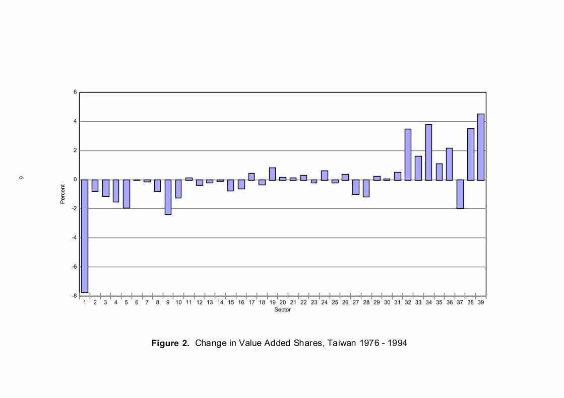
Figure 2. Change in Value Added Shares, Taiwan 1976 - 1994

7

-80

-60

-40

-20

0

20

40 M

anuf

actu

ring

0

50

100

150

200

250

300

Serv

ices

Agric Minerals Mfg Const Utilities Transport Trade Services All Ind

Manufacturing Services

Figure 3. Percentage Change in Consumption of Manufactures and Services per unit Output,Taiwan 1976 -1994

8

the other hand, consistently increased its share of GDP from 27.0% in 1976 to 41.3% in 1994.

Minerals, Construction, Utilities, Transport and Trade retained relatively constant shares of

GDP over the period.

The shift from primary to tertiary activities can also be clearly seen in Figure 2, which shows the

change in value added shares by sector over the period 1976 to 1994. All primary activities

decline in share with Agricultural products and livestock experiencing the largest decline from

10.5 to 2.8 percent. Conversely, all service sectors except Public administrative services increase

their shares. In aggregate terms, primary activities decreased their value added share by 2.7%,

manufacturing fell by 0.3%, and services increased their share by 2.1%.

Figure 3 shows the percentage change in the consumption of services and manufactures per unit

of output for a group of more highly aggregated sectors. In all cases, consumption of services has

increased, and except for Minerals, Manufacturing and Construction, consumption of

manufactures has decreased. Over all industries, the consumption of services increased by 94.5%

and the consumption of manufactures decreased by 11.4% over the sample period.

The Taiwanese experience is mirrored in studies of international comparative analysis using

input-output tables from countries at all levels of development which have demonstrated that

over the course of the transition from low- to high-income there is a strong shift in value-added

from primary production to manufacturing and nontradables, and, at high income levels the share

of manufacturing declines and of services increases (Syrquin and Chenery [37]). This finding is

consistent with the earlier work of Clark [16] and Fisher [21] predicting the emergence of the

“service economy” and the "de-industrialisation" of highly developed countries, which they

attributed to the relatively higher income elasticities of demand for services. This became known

as the Clark-Fisher hypothesis. Despite later studies questioning Clark and Fisher’s demand-side

explanation, Clark and Fisher were at least correct in highlighting that structural change in the

economic system accompanies the process of economic development.

2.2 Interindustry linkages

Surprisingly, much less attention has been given to the analysis of the evolution of interindustry

linkages over the transition, even though it was more than 40 years ago that Chenery and

Watanabe [13] demonstrated the use of IO analysis in identifying and comparing patterns of

interdependence among sectors. It was found then that during the process of development, the

9

total use of intermediate inputs relative to gross output increases and its composition shifts as the

importance of primary products declines and of heavy industrial products and nontradables,

particularly services, increases. What is important to note here is that these changes in the

structure of production were found to be attributable not so much to changes in the composition

of final output, as predicted by the Clark-Fisher hypothesis, but rather to increases in the density

of the input-output matrices as the economy evolves from relatively simple handicrafts

production to a more complex, factory-based system with a higher degree of fabrication.

Deutsch and Syrquin [18], in an analysis of structural change inspired by Chenery and Watanabe

[13], studied the relationship between economic development and structural change for 30

countries, of which Taiwan was one, over the period 1950–75, making use of IO tables, each of

which, for the purpose of comparison, was condensed to 10 sectors. As expected, it was

discovered that economic development is associated with an increasing share of intermediate

goods in total output.3 Korea and Taiwan, as countries which experienced rapid industrialisation,

were notable for the large increase in demand for intermediates that they experienced. The

analytical tools relied upon by Deutsch and Syrquin [18, p. 448] were measures of sectoral

linkages, especially the forward linkage index, which is the ratio of intermediate to total demand.

It has been shown that the internal connectedness or complexity of the economic structure,

measured in terms of the strength of intermediate linkages, increased systematically in Taiwan

during the initial phases of its development. Its input-output coefficients increased faster in

manufacturing than elsewhere, and, by the mid-1970s, Taiwan had attained the same overall

level of industrial interdependence as Japan (Albala-Bertrand [2]). Similarly, Brown and Hooper

[7] have shown that over the period 1976 to 1991, Taiwan’s dependency of tradable goods

sectors on non-tradables increased significantly, again suggesting a more complex or

‘roundabout’ production structure as the economy developed.

2.3 Sources of structural change

Other studies indicate that changes in Taiwan’s economic structure are attributable more to

changes in the pattern of final demand than to changes in interindustry linkages. Wang, Sun and

Chou [39] decomposed structural change into its sources, which are final demand, export

expansion, import substitution and technological change. Using Taiwan’s IO tables for 1979 and

3 This reaffirmed an earlier finding to the same effect by Chenery [10; 11].

10

1984 they found the relative contributions to structural change were: 47.84 percent for demand;

38.04 percent for exports; 2.11 percent for import substitution; and, 5.21 percent for

technological change (Wang, Sun & Chou [39, p.393–94]). The residual was composed of cross-

terms of the sources of structural change. These findings suggest that most of the change in the

structure of the Taiwanese economy is attributable to changes in final demand rather than inter-

industry relationships.

Wang [40;41] also applied a multiplicative decomposition method within an IO framework.

Structural change was identified using the rowscaler method pioneered by Carter [8] and

Feldman & Palmer [20] in their analyses of structural change in the United States. The main

purpose of this method is to estimate the extent to which changes in the composition of output

can be attributed to changes in IO coefficients (rowscalar) versus final demand (columnscalar).4

Applying this method to Taiwan over the period using IO tables comprising 29 sectors for the

years 1966, 1976, 1981, 1986, and 1991, Wang discovered large changes in intermediate

transaction and final demand coefficients for the miscellaneous services sector, and significant

changes in other sectors notable for producing intermediate requirements viz., electronics,

transport equipment and machinery. This is to be expected of a developing economy becoming

more interconnected.

2.4 Hollowing-out

However, it is noteworthy that the shifts in Taiwan’s economic structure have also been

accompanied by increased outsourcing of inputs, as shown in Figure 4. There have been massive

increases in import levels per unit output for Textile mill products (4597.3%), Miscellaneous

chemical products (3624.3%), Tobacco (1476.6%), Wearing apparel and accessories (559.6%)

and Household electrical appliances (372.9%). Over all industries, the average increase in

imports per unit output was 12.3% between 1976 and 1991.

It is also significant that from the mid-1980’s Taiwanese capital began relocating offshore,

associated with a sizeable appreciation of the currency (NT$) and rising real wages (Li and Hu

[24]). This relocation process became of concern to policy makers who saw it as a source of

4 For an application of a similar, biproportional method to China using IO tables for 1987 and 1995, see

Andreosso-O’Callaghan and Yue [4].

11

-80

-60

-40

-20

0

20

40 M

anuf

actu

ring

0

50

100

150

200

250

300

Serv

ices

Agric Minerals Mfg Const Utilities Transport Trade Services All Ind

Manufacturing Services

Figure 3. Percentage Change in Consumption of Manufactures and Services per unit Output,Taiwan 1976 -1994

12

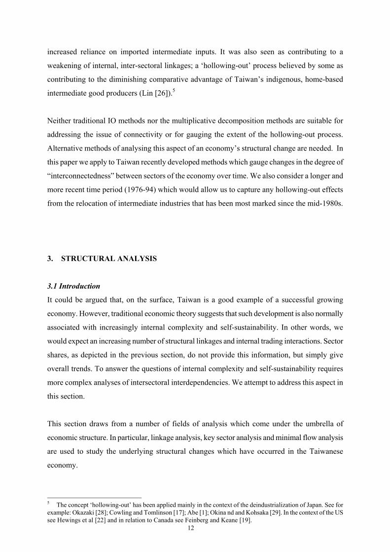
increased reliance on imported intermediate inputs. It was also seen as contributing to a

weakening of internal, inter-sectoral linkages; a ‘hollowing-out’ process believed by some as

contributing to the diminishing comparative advantage of Taiwan’s indigenous, home-based

intermediate good producers (Lin [26]).5

Neither traditional IO methods nor the multiplicative decomposition methods are suitable for

addressing the issue of connectivity or for gauging the extent of the hollowing-out process.

Alternative methods of analysing this aspect of an economy’s structural change are needed. In

this paper we apply to Taiwan recently developed methods which gauge changes in the degree of

“interconnectedness” between sectors of the economy over time. We also consider a longer and

more recent time period (1976-94) which would allow us to capture any hollowing-out effects

from the relocation of intermediate industries that has been most marked since the mid-1980s.

3. STRUCTURAL ANALYSIS

3.1 Introduction

It could be argued that, on the surface, Taiwan is a good example of a successful growing

economy. However, traditional economic theory suggests that such development is also normally

associated with increasingly internal complexity and self-sustainability. In other words, we

would expect an increasing number of structural linkages and internal trading interactions. Sector

shares, as depicted in the previous section, do not provide this information, but simply give

overall trends. To answer the questions of internal complexity and self-sustainability requires

more complex analyses of intersectoral interdependencies. We attempt to address this aspect in

this section.

This section draws from a number of fields of analysis which come under the umbrella of

economic structure. In particular, linkage analysis, key sector analysis and minimal flow analysis

are used to study the underlying structural changes which have occurred in the Taiwanese

economy.

5 The concept ‘hollowing-out’ has been applied mainly in the context of the deindustrialization of Japan. See for example: Okazaki [28]; Cowling and Tomlinson [17]; Abe [1]; Okina nd and Kohsaka [29]. In the context of the US see Hewings et al [22] and in relation to Canada see Feinberg and Keane [19].

13

3.2 Linkage Analysis

The concept of key sectors is generally regarded as initially being conceived with the work of

Rasmussen [31] and Hirschman [23]. West [42] develops a technique for determining the effects

of coefficient changes on the multiplier values which is demonstrated on an 11-sector table for

South Australia. More recently, Sonis, Hewings and Guo [35] provide a theoretical framework

for key sector analysis based on a minimum information approach which is then applied to

Chinese IO tables for 1987 and 1990. Central to the concept of key sectors is the notion of

backward and forward linkages. The aim of linkage analysis is to measure the potential stimulus

to other activities from investment in any sector, and to identify those sectors which create an

above average stimulus to the rest of the economy.

3.2.1 Background linkages

The numerator in the backward linkage index for sector j ( L j ) is essentially an output multiplier

and denotes the average stimulus imparted to other sectors by a unit's worth of demand for sector

j's output. In order to make comparisons between sectors, a normalisation procedure is carried

out by dividing by the average stimulus to the whole economy when all sectors' final demands

are increased by unity. If 1 > L j , investment in sector j yields above average multiplier effects,

while if 1 < L j , investment in sector j produces below average multiplier effects.

These linkages can be disaggregated across the n input sectoral components which provides

information on the distributional effects of the initial investment stimulus across the n sectors in

the economy. A useful dichotomy of disaggregated linkage effects is the self and non-self

contributions. In the former, changes in output can be traced to intrasectoral changes within the

industry itself, while in the latter the changes impact on other sectors.

Selecting sectors with a high index on its own is insufficient for policy and planning purposes,

since only one or two sectors may stand to gain from the stimulus. Ideally, we require any

stimulus to sector j to spread as widely as possible throughout the economy. A measure of this

backward spread is the coefficient of variation. Normalising gives the backward spread index

(V j ). A low V j means that investment in sector j would stimulate a large number of other

sectors, while a high V j indicates the stimulus would only have localised effects. A key

backward sector is defined as one which has both a high backward linkage index and a low

spread index.

14

3.2.2 Forward linkages

Backward linkages only provide part of the story. Backward linkages provide information on the

effects of investment in a given industry on upstream activities in a demand driven sense, i.e.

through increased demands for other sector inputs. But what about downstream activities? The

increased output in sector j may alleviate bottlenecks to supply to other industries which can in

turn increase production, or alternatively all the increased output may be exported. To measure

the effect of investment in sector j on these downstream activities, forward linkages and spread

effects can be calculated.

The basic idea of forward linkages is to trace the output increases which occur or might occur in

using industries when there is a change in the sector supplying inputs, in contrast to backward

linkages which trace the output increases which occur in supplying industries when there is a

change in the sector using its products as inputs. The forward linkage index is calculated from

the supply-side model in an analogous manner to the backward linkage index.

The forward linkages are now defined in terms of input multipliers, which measure the effect on

total output of all sectors associated with a unit change in the primary inputs of sector i. For

example, we may want to decide where to place an additional investment in primary factors

(labour or capital) so that it would be most beneficial to the total economy, in terms of potential

for supporting expanded output.

3.2.3 Backward and forward linkages for Taiwan

The backward and forward linkages for Taiwan are given in Tables 2 and 3, and in Figures 5 and

6 for a more aggregated set of sectors.

From Figure 5, it can be seen that only three sectors can be classified as having above average

(i.e. above 1) backward linkages over the full sample period: Construction, Manufacturing and

Utilities. Utilities has the highest ranking of all sectors in terms of backward linkages in 1976 but

quickly drops to third place by 1986. Construction attains first place in 1981 and retains that

position for the remainder of the sample period. Manufacturing keeps a consistent second

ranking for the whole sample period. It is also of interest to note that Agriculture’s backward

linkage index gradually increases over the period, becoming greater than one in 1989. Minerals

has the lowest backward index over the whole period. Figure 6 shows that the sectors with above

15

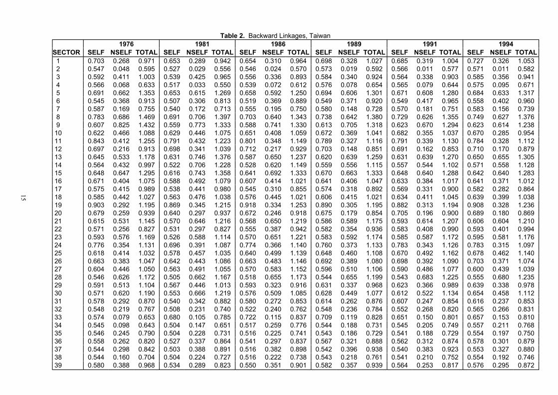
Table 2. Backward Linkages, Taiwan 1976 1981 1986 1989 1991 1994

SECTOR SELF NSELF TOTAL SELF NSELF TOTAL SELF NSELF TOTAL SELF NSELF TOTAL SELF NSELF TOTAL SELF NSELF TOTAL 1 0.703 0.268 0.971 0.653 0.289 0.942 0.654 0.310 0.964 0.698 0.328 1.027 0.685 0.319 1.004 0.727 0.326 1.053 2 0.547 0.048 0.595 0.527 0.029 0.556 0.546 0.024 0.570 0.573 0.019 0.592 0.566 0.011 0.577 0.571 0.011 0.582 3 0.592 0.411 1.003 0.539 0.425 0.965 0.556 0.336 0.893 0.584 0.340 0.924 0.564 0.338 0.903 0.585 0.356 0.941 4 0.566 0.068 0.633 0.517 0.033 0.550 0.539 0.072 0.612 0.576 0.078 0.654 0.565 0.079 0.644 0.575 0.095 0.671 5 0.691 0.662 1.353 0.653 0.615 1.269 0.658 0.592 1.250 0.694 0.606 1.301 0.671 0.608 1.280 0.684 0.633 1.317 6 0.545 0.368 0.913 0.507 0.306 0.813 0.519 0.369 0.889 0.549 0.371 0.920 0.549 0.417 0.965 0.558 0.402 0.960 7 0.587 0.169 0.755 0.540 0.172 0.713 0.555 0.195 0.750 0.580 0.148 0.728 0.570 0.181 0.751 0.583 0.156 0.739 8 0.783 0.686 1.469 0.691 0.706 1.397 0.703 0.640 1.343 0.738 0.642 1.380 0.729 0.626 1.355 0.749 0.627 1.376 9 0.607 0.825 1.432 0.559 0.773 1.333 0.588 0.741 1.330 0.613 0.705 1.318 0.623 0.670 1.294 0.623 0.614 1.238 10 0.622 0.466 1.088 0.629 0.446 1.075 0.651 0.408 1.059 0.672 0.369 1.041 0.682 0.355 1.037 0.670 0.285 0.954 11 0.843 0.412 1.255 0.791 0.432 1.223 0.801 0.348 1.149 0.789 0.327 1.116 0.791 0.339 1.130 0.784 0.328 1.112 12 0.697 0.216 0.913 0.698 0.341 1.039 0.712 0.217 0.929 0.703 0.148 0.851 0.691 0.162 0.853 0.710 0.170 0.879 13 0.645 0.533 1.178 0.631 0.746 1.376 0.587 0.650 1.237 0.620 0.639 1.259 0.631 0.639 1.270 0.650 0.655 1.305 14 0.564 0.432 0.997 0.522 0.706 1.228 0.528 0.620 1.149 0.559 0.556 1.115 0.557 0.544 1.102 0.571 0.558 1.128 15 0.648 0.647 1.295 0.616 0.743 1.358 0.641 0.692 1.333 0.670 0.663 1.333 0.648 0.640 1.288 0.642 0.640 1.283 16 0.671 0.404 1.075 0.588 0.492 1.079 0.607 0.414 1.021 0.641 0.406 1.047 0.633 0.384 1.017 0.641 0.371 1.012 17 0.575 0.415 0.989 0.538 0.441 0.980 0.545 0.310 0.855 0.574 0.318 0.892 0.569 0.331 0.900 0.582 0.282 0.864 18 0.585 0.442 1.027 0.563 0.476 1.038 0.576 0.445 1.021 0.606 0.415 1.021 0.634 0.411 1.045 0.639 0.399 1.038 19 0.903 0.292 1.195 0.869 0.345 1.215 0.918 0.334 1.253 0.890 0.305 1.195 0.882 0.313 1.194 0.908 0.328 1.236 20 0.679 0.259 0.939 0.640 0.297 0.937 0.672 0.246 0.918 0.675 0.179 0.854 0.705 0.196 0.900 0.689 0.180 0.869 21 0.615 0.531 1.145 0.570 0.646 1.216 0.568 0.650 1.219 0.586 0.589 1.175 0.593 0.614 1.207 0.606 0.604 1.210 22 0.571 0.256 0.827 0.531 0.297 0.827 0.555 0.387 0.942 0.582 0.354 0.936 0.583 0.408 0.990 0.593 0.401 0.994 23 0.593 0.576 1.169 0.526 0.588 1.114 0.570 0.651 1.221 0.583 0.592 1.174 0.585 0.587 1.172 0.595 0.581 1.176 24 0.776 0.354 1.131 0.696 0.391 1.087 0.774 0.366 1.140 0.760 0.373 1.133 0.783 0.343 1.126 0.783 0.315 1.097 25 0.618 0.414 1.032 0.578 0.457 1.035 0.640 0.499 1.139 0.648 0.460 1.108 0.670 0.492 1.162 0.678 0.462 1.140 26 0.663 0.383 1.047 0.642 0.443 1.086 0.663 0.483 1.146 0.692 0.389 1.080 0.698 0.392 1.090 0.703 0.371 1.074 27 0.604 0.446 1.050 0.563 0.491 1.055 0.570 0.583 1.152 0.596 0.510 1.106 0.590 0.486 1.077 0.600 0.439 1.039 28 0.546 0.626 1.172 0.505 0.662 1.167 0.518 0.655 1.173 0.544 0.655 1.199 0.543 0.683 1.225 0.555 0.680 1.235 29 0.591 0.513 1.104 0.567 0.446 1.013 0.593 0.323 0.916 0.631 0.337 0.968 0.623 0.366 0.989 0.639 0.338 0.978 30 0.571 0.620 1.190 0.553 0.666 1.219 0.576 0.509 1.085 0.628 0.449 1.077 0.612 0.522 1.134 0.654 0.458 1.112 31 0.578 0.292 0.870 0.540 0.342 0.882 0.580 0.272 0.853 0.614 0.262 0.876 0.607 0.247 0.854 0.616 0.237 0.853 32 0.548 0.219 0.767 0.508 0.231 0.740 0.522 0.240 0.762 0.548 0.236 0.784 0.552 0.268 0.820 0.565 0.266 0.831 33 0.574 0.079 0.653 0.680 0.105 0.785 0.722 0.115 0.837 0.709 0.119 0.828 0.651 0.150 0.801 0.657 0.153 0.810 34 0.545 0.098 0.643 0.504 0.147 0.651 0.517 0.259 0.776 0.544 0.188 0.731 0.545 0.205 0.749 0.557 0.211 0.768 35 0.546 0.245 0.790 0.504 0.228 0.731 0.516 0.225 0.741 0.543 0.186 0.729 0.541 0.188 0.729 0.554 0.197 0.750 36 0.558 0.262 0.820 0.527 0.337 0.864 0.541 0.297 0.837 0.567 0.321 0.888 0.562 0.312 0.874 0.578 0.301 0.879 37 0.544 0.298 0.842 0.503 0.388 0.891 0.516 0.382 0.898 0.542 0.396 0.938 0.540 0.383 0.923 0.553 0.327 0.880 38 0.544 0.160 0.704 0.504 0.224 0.727 0.516 0.222 0.738 0.543 0.218 0.761 0.541 0.210 0.752 0.554 0.192 0.746 39 0.580 0.388 0.968 0.534 0.289 0.823 0.550 0.351 0.901 0.582 0.357 0.939 0.564 0.253 0.817 0.576 0.295 0.872

16

Table 3. Forward Linkages, Taiwan 1976 1981 1986 1989 1991 1994

SECTOR SELF NSELF TOTAL SELF NSELF TOTAL SELF NSELF TOTAL SELF NSELF TOTAL SELF NSELF TOTAL SELF NSELF TOTAL 1 0.659 0.588 1.247 0.647 0.551 1.198 0.615 0.551 1.167 0.650 0.526 1.176 0.643 0.480 1.123 0.683 0.475 1.158 2 0.513 0.791 1.304 0.521 0.869 1.390 0.514 0.865 1.378 0.534 0.861 1.394 0.531 0.856 1.386 0.536 0.868 1.404 3 0.555 0.127 0.682 0.534 0.169 0.703 0.523 0.222 0.746 0.544 0.177 0.721 0.529 0.132 0.661 0.550 0.118 0.668 4 0.530 1.171 1.701 0.512 1.310 1.822 0.507 1.340 1.847 0.536 1.301 1.837 0.530 1.308 1.839 0.541 1.260 1.800 5 0.647 0.163 0.810 0.647 0.192 0.839 0.619 0.186 0.805 0.647 0.198 0.845 0.630 0.157 0.786 0.643 0.149 0.792 6 0.511 0.020 0.531 0.502 0.014 0.516 0.488 0.021 0.510 0.512 0.020 0.531 0.515 0.007 0.522 0.525 0.008 0.532 7 0.550 0.005 0.555 0.535 0.003 0.537 0.521 0.005 0.526 0.540 0.003 0.543 0.534 0.001 0.536 0.548 0.001 0.549 8 0.734 0.370 1.104 0.684 0.398 1.082 0.661 0.412 1.073 0.687 0.361 1.048 0.683 0.287 0.970 0.704 0.228 0.932 9 0.569 0.092 0.661 0.554 0.076 0.629 0.553 0.083 0.636 0.570 0.088 0.659 0.584 0.088 0.673 0.586 0.101 0.687 10 0.583 0.228 0.811 0.623 0.230 0.853 0.612 0.198 0.809 0.626 0.255 0.880 0.640 0.292 0.932 0.629 0.361 0.991 11 0.790 0.607 1.397 0.782 0.675 1.458 0.753 0.656 1.410 0.735 0.671 1.406 0.742 0.669 1.411 0.737 0.683 1.420 12 0.653 1.135 1.788 0.691 1.179 1.870 0.669 1.138 1.807 0.654 1.164 1.818 0.648 1.111 1.759 0.667 1.040 1.707 13 0.605 0.765 1.369 0.624 0.718 1.342 0.552 0.765 1.317 0.577 0.756 1.333 0.592 0.647 1.239 0.611 0.580 1.190 14 0.529 0.774 1.303 0.517 0.859 1.376 0.497 0.832 1.329 0.520 0.790 1.311 0.523 0.763 1.286 0.536 0.705 1.242 15 0.608 0.235 0.843 0.609 0.249 0.858 0.603 0.255 0.858 0.624 0.310 0.934 0.608 0.323 0.931 0.604 0.378 0.981 16 0.629 0.591 1.220 0.582 0.553 1.135 0.571 0.596 1.167 0.597 0.588 1.184 0.594 0.589 1.183 0.603 0.556 1.159 17 0.539 0.793 1.332 0.533 0.889 1.422 0.513 0.955 1.468 0.534 0.917 1.452 0.533 0.911 1.444 0.547 0.840 1.387 18 0.549 0.536 1.085 0.557 0.491 1.047 0.542 0.502 1.044 0.565 0.511 1.075 0.595 0.539 1.134 0.600 0.575 1.175 19 0.847 0.704 1.551 0.861 0.682 1.542 0.863 0.705 1.569 0.829 0.676 1.504 0.827 0.671 1.498 0.854 0.668 1.522 20 0.637 0.906 1.542 0.633 0.868 1.501 0.632 0.824 1.455 0.628 0.786 1.415 0.661 0.776 1.437 0.648 0.752 1.400 21 0.576 0.521 1.097 0.564 0.432 0.996 0.534 0.368 0.902 0.545 0.363 0.909 0.556 0.396 0.953 0.569 0.371 0.941 22 0.535 0.170 0.705 0.525 0.167 0.692 0.522 0.231 0.753 0.542 0.165 0.707 0.546 0.157 0.703 0.557 0.149 0.707 23 0.556 0.073 0.629 0.520 0.076 0.596 0.536 0.090 0.626 0.542 0.064 0.607 0.548 0.068 0.616 0.559 0.077 0.636 24 0.728 0.033 0.761 0.689 0.041 0.730 0.728 0.057 0.785 0.708 0.056 0.763 0.735 0.058 0.793 0.736 0.055 0.790 25 0.579 0.431 1.009 0.572 0.367 0.939 0.602 0.403 1.005 0.603 0.339 0.942 0.629 0.379 1.008 0.638 0.367 1.005 26 0.622 0.131 0.752 0.636 0.064 0.700 0.624 0.108 0.732 0.644 0.091 0.734 0.655 0.088 0.743 0.660 0.086 0.747 27 0.566 0.101 0.667 0.558 0.080 0.638 0.536 0.087 0.623 0.555 0.099 0.654 0.554 0.110 0.663 0.564 0.129 0.693 28 0.511 0.048 0.559 0.500 0.058 0.557 0.487 0.120 0.607 0.507 0.087 0.594 0.509 0.111 0.620 0.522 0.107 0.629 29 0.554 0.937 1.491 0.561 0.896 1.457 0.557 0.859 1.416 0.587 0.846 1.434 0.584 0.846 1.430 0.601 0.793 1.394 30 0.535 0.266 0.801 0.548 0.250 0.798 0.542 0.305 0.846 0.585 0.356 0.941 0.574 0.400 0.974 0.615 0.380 0.995 31 0.541 0.358 0.899 0.535 0.350 0.884 0.546 0.362 0.908 0.572 0.386 0.958 0.569 0.332 0.901 0.579 0.327 0.906 32 0.513 0.290 0.803 0.503 0.285 0.789 0.491 0.337 0.828 0.510 0.297 0.808 0.518 0.343 0.861 0.531 0.325 0.856 33 0.538 0.606 1.144 0.673 0.768 1.441 0.679 0.794 1.472 0.660 0.544 1.204 0.610 0.687 1.298 0.617 0.678 1.296 34 0.511 0.117 0.628 0.499 0.047 0.546 0.486 0.086 0.572 0.506 0.085 0.592 0.511 0.179 0.690 0.524 0.165 0.688 35 0.511 0.328 0.839 0.498 0.171 0.670 0.485 0.175 0.661 0.505 0.160 0.666 0.507 0.137 0.644 0.520 0.136 0.656 36 0.523 0.665 1.188 0.522 0.772 1.294 0.508 0.761 1.270 0.528 0.766 1.294 0.527 0.749 1.275 0.543 0.779 1.323 37 0.510 0.000 0.510 0.498 0.000 0.498 0.485 0.000 0.485 0.505 0.000 0.505 0.507 0.000 0.507 0.519 0.000 0.519 38 0.510 0.046 0.556 0.499 0.045 0.544 0.485 0.052 0.538 0.506 0.056 0.562 0.508 0.048 0.556 0.521 0.049 0.570 39 0.544 0.582 1.125 0.529 0.582 1.111 0.517 0.534 1.051 0.542 0.517 1.060 0.529 0.487 1.017 0.542 0.413 0.955

17

0.6

0.7

0.8

0.9

1

1.1

1.2

1.3

1.4

1976 1981 1986 1989 1991 1994

Agric

Minerals

Mfg

Const

Utilities

Transport

Trade

Services

Figure 5. Total Backward Linkages, Taiwan 1976 - 1994

18

0.4

0.6

0.8

1

1.2

1.4

1.6

1976 1981 1986 1989 1991 1994

Agric

Minerals

Mfg

Const

Utilities

Transport

Trade

Services

Figure 6. Total Forward Linkages, Taiwan 1976 - 1994

19

average forward linkages are Minerals, Utilities and Agriculture.

Study of Table 2 shows that the self-component of the backward linkage in virtually all cases

(the notable exception is Construction) is greater than the non-self component. This indicates

that a stimulus to the industry impacts more on intrasectoral firms within that industry than firms

outside that industry, indicating a high degree of integration within industry structures. This is

also true, but to a less obvious extent, for the forward linkages shown in Table 3. Further analysis

of these tables indicates that the proportion of self-component within each sector does not change

much over time, so that the degree of integration appears relatively constant.

3.3 Key Sector Analysis

Backward and forward linkages are central to the concept of key sectors. A key sector is defined

as one which exhibits both high backward and forward linkage indexes and low backward and

forward spread indexes (West [42]).

If we collect the backward linkage indexes at time t in the n-element row vector Lt , and the

forward linkage indexes in the n-element column vector Ltr , then we can define the Linkage

Product Matrix as L L = M tttr . The elements of M are uniquely associated with each

combination of backward and forward linkage indices; large elements will be associated with

large backward and forward linkages, and small elements will be associated with small backward

and forward linkages. In graph theoretic terms, the matrix depicts an economic landscape of

linkages which will highlight the strengths and weaknesses of the economic interactions between

sectors.

3.3.1 Spread indices and the Key Sector Matrix

To completely identify the key sectors, we also need to take into account the spread indices.

Noting that the mean of the spread indices is unity, an adjusted set of indices symmetric to the

original set about unity can be constructed by V - i 2 = U tt ′ and V - i 2 = U ttrr , where V t is the

n-element row vector of backward spread indices, V tr the n-element column vector of forward

spread indices, and i denotes an n-element column vector of ones. Unlike V j and V ir which

ideally should by small, we want U j and U ir to be large to maximise the spread effects of a

stimulus to sector j. The companion matrix to M, termed the Spread Product Matrix, is now

20

defined as U U = S tttr , from which a Key Sector Matrix can be constructed as S M = K ttt •

where • denotes an element by element product.

The key sector matrix provides a unique insight into the underlying structural core and highlights

the key interactions in terms of their contribution to the direct and indirect flow-ons to the rest of

the economy. Large elements reflect strong interconnections and indicate sectoral links which

form a fundamental bonded core of the economy.

The K matrix exhibits some interesting properties and can be analysed and depicted in a number

of ways. For example, all the rows are proportional to each other and similarly for the columns.

The matrix can therefore be rank-sorted by both rows and columns to provide a hierarchial

picture of key sectors. In this paper, a simpler approach is taken. For the six time periods under

consideration, the K matrix is depicted as a contour map which provides a clear visual

representation of the similarities and differences in the linkage structure of the Taiwanese

economy over the twenty-year time span. These are given in Figure 7.

In each of the maps, darker shading represents stronger linkages. Intersectoral links are defined

by the intersection of grid lines with the columns representing backward linkages and the rows

forward linkages. Thus, in 1976, for example, Wearing apparel and accessories (sector 9) has

the strongest backward linkages in terms of direct and indirect inputs, and Chemical materials

(sector 12) has the strongest forward linkages in terms of other industry uses. Plastic products

(sector 15) ranks as the second most significant sector in terms of backward linkages in 1976.

From a comparison of the landscape maps in Figure 7 over time, it can be seen that density

reaches a peak in 1981 and thereafter there is a noticeable decline. While Minerals (sector 4) and

Chemical materials (sector 12) retain a significant key sector status in terms of forward linkages,

and Wearing apparel and accessories (sector 9) and Plastic products (sector 15) retain

significant backward linkage status over the period 1976 to 1994, their status had noticeably

diminished by 1994. The landscape maps appear to be becoming less dense over time, implying a

decrease in the level and complexity of the internal structure.

This trend is verified by the finding that the largest key sector index has progressively fallen over

the period from 4.189 in 1976 to 3.924 in 1994.

21

1 2 3 4 5 6 7 8 9 10 11 12 13 14 15 16 17 18 19 20 21 22 23 24 25 26 27 28 29 30 31 32 33 34 35 36 37 38 39

Backward Linkages

1976

1986

Figure 7a. Key Sector Maps, Taiwan

123456789101112131415161719192021222324252627282930313233343536373839

1981

22

1 2 3 4 5 6 7 8 9 10 11 12 13 14 15 16 17 18 19 20 21 22 23 24 25 26 27 28 29 30 31 32 33 34 35 36 37 38 39

Backward Linkages

1989

1994

Figure 7b. Key Sector Maps, Taiwan

123456789101112131415161719192021222324252627282930313233343536373839

1991

23

3.3.2 Intermediate requirements and hollowing-out

Further evidence to support the observation of diminishing internal complexity in the Taiwanese

economy can be seen in Figure 8 which shows total direct and direct plus indirect requirements

coefficients. After the growth spurt from 1976 to 1981, the total intermediate requirements,

which measures the volume of intersectoral flows, dips back to the 1976 levels in 1989 before

recovering slightly in 1991 and falling again in 1994. Moreover, the direct and indirect

requirements are falling faster than the direct requirements (average growth rates of -0.52 per

cent for direct requirements compared to -1.62 per cent for direct and indirect requirements over

the period 1976 to 1994), which indicates a definite thinning of the indirect intersectoral core

which is a leading indicator of the internal complexity of the economy.

Table 4 gives the sectoral percentage changes in direct and indirect requirements over the sample

period. Only 16 of the 39 sectors experienced positive growth in direct inputs and in all these

cases the indirect inputs grow at a slower rate than direct inputs. In other words, the backward

linkages in these sectors have not kept pace with direct purchases. The most noticeable of these

sectors were Finance and insurance services (sector 33) and Real estate services (sector 34)

where direct inputs increased by approximately 119 per cent and indirect inputs increases by

only 9 per cent. The remaining 23 sectors experienced a decline in intermediate input shares

which indicates either greater outsourcing of inputs and/or disproportionate increasing returns to

labour and capital, and/or increasing agglomeration of intra-industry firms within sectors. The

former is supported by the shift from primary and secondary activities to service industries as

shown from Figures 1 to 3. The latter argument is supported by close examination of Table 2

which shows that in only 16 sectors the non-self backward linkage component outgrew the self

component over the period 1976 to 1994, and in 13 cases, the growth in self component was

positive while the growth in non-self component was negative. Over all industries, direct

requirements fell by an average of 0.5 per cent while indirect requirements fell by 2.0 per cent

over the period 1976 to 1994. A similar story can be told with respect to the intermediate

demands.

This apparent decline in density in a developing economy is not a unique observation. A similar

phenomenon has been observed for the Japanese economy, a procedure referred to as a

"hollowing out" effect (Okazaki [28] ; Abe [1]; Okina and Kohsaka [29]). The process can be

likened to scooping out the inside of a large fruit; the size of the fruit remained the same or

24

17

17.5

18

18.5

19

19.5 D

irect

70

71

72

73

74

75

76

77

78

Dire

ct &

Indi

rect

1976 1981 1986 1989 1991 1994

Direct Direct & Indirect

Figure 8. Total Intermediate Requirements

25

slowly increases but its density decreases, an analogy to the loss of flows between sectors within

the intermediary part of the economy. Hewings et al. [22] observed a similar trend in the

Chicago economy and West [43] in the Queensland economy.

3.4 Measuring connectivity

3.4.1 Qualitative I-O analysis

Another variation of graph theoretic applications to analysing the economic structure of an

economy can be derived from qualitative input-output analysis (QIOA) (Bon [6]). This procedure

converts the input-output matrix into a Boolean matrix to facilitate and enable some

generalisations to be made about the degree of connectivity of the system. While quantitative

input-output analysis is concerned with value information, QIOA emphasises the

interdependencies within the economy. Like a road map, it highlights the main features of

interest but treats as background those characteristics not crucial to the purpose at hand. Through

simplification, less is held in view so that more can be understood of what is retained.

The basic concept of classical QIOA consists of the correspondence mapping of the entries of the

input-output table T into a qualitative binary adjacency matrix W according to an arbitrarily

predefined filter rate:

m , 1, =j i, filter < t if 0filter t if 1

= wij

ijij K∀

≥

After the binarisation step, several graph-theoretical methods can be applied to the adjacency

matrix which trace the connections contained therein. To obtain the complete structure, both

direct and indirect linkages are taken into account. As shown by Busacker and Saaty [5] the

indirect links can be traced to the kth step by applying the equation Wk = W Wk-1, where the

power sequence of the Wk shows how many paths of length k exist between the sectors. For

example, the ilth entry in W2 contains a 1 if and only if both the elements wij and wjl are 1 thus

reflecting a 2-step connection between sectors i and l via sector j. Additionally a so-called

dependency matrix D can be derived by Boolean summation (i.e. 1 + 1 = (#)1) of the matrices

Wk. Thus an entry dij = 1 shows that there exists a linked flow from sector i to j no matter how

many steps are taken which makes D a 'qualitative' inverse of the original table.

26

Table 4. Percentage Change in Intermediate Requirements and Demands, Taiwan 1976 - 1994 Sector Intermediate Requirements Intermediate Demands

Direct Indirect Total Direct Indirect Total 1 19.6 3.1 6.6 -10.5 -8.1 -8.9 2 -20.2 -2.9 -3.8 -2.2 9.8 5.7 3 -9.4 -7.3 -7.8 -11.0 -2.5 -3.9 4 35.8 1.3 4.2 7.0 2.6 3.8 5 -8.3 -2.3 -4.2 0.5 -5.2 -4.1 6 15.7 0.5 3.5 -8.6 -1.6 -1.7 7 -13.8 -1.8 -3.8 -30.7 -0.7 -2.8 8 -10.6 -6.9 -7.9 -27.7 -12.4 -17.2 9 -15.2 -14.9 -15.0 13.5 0.1 2.0 10 -32.3 -4.6 -13.7 40.2 12.8 19.9 11 -13.7 -12.5 -12.8 -3.3 1.0 -0.3 12 -10.9 -3.4 -5.2 -2.4 -7.8 -6.3 13 11.5 8.0 9.1 -13.8 -15.0 -14.7 14 31.4 4.2 11.4 -19.8 0.8 -6.5 15 -1.1 -3.2 -2.6 30.0 9.0 14.3 16 -9.6 -6.6 -7.4 1.8 -10.3 -6.8 17 -34.8 -2.3 -14.1 1.3 2.6 2.2 18 -2.7 0.3 -0.6 6.2 6.3 6.3 19 6.7 0.0 1.8 -1.0 -4.9 -3.7 20 -14.5 -7.1 -8.9 -6.0 -13.1 -10.9 21 10.3 1.6 3.9 -19.5 -14.3 -15.9 22 53.9 10.5 18.2 0.6 -2.0 -1.6 23 -1.8 -0.7 -1.0 -4.6 -0.1 -0.7 24 -4.0 -4.7 -4.5 4.2 1.2 1.9 25 20.3 4.9 8.7 -6.6 -0.3 -2.3 26 0.3 1.1 0.9 -2.6 -2.6 -2.6 27 -1.6 -3.0 -2.7 -3.4 3.0 2.0 28 7.0 2.4 3.7 115.1 3.5 10.3 29 -16.0 -11.6 -12.9 -7.6 -8.6 -8.3 30 -7.6 -8.3 -8.1 56.3 12.6 21.8 31 -2.9 -3.8 -3.6 -5.1 0.3 -1.1 32 26.0 2.4 6.6 17.2 1.3 4.6 33 119.9 9.3 21.9 14.5 9.7 11.2 34 118.8 9.0 17.5 40.1 3.7 7.6 35 -14.9 -5.0 -6.6 -58.0 -12.8 -23.3 36 23.7 1.4 5.4 10.8 8.4 9.2 37 8.9 1.2 2.8 0.0 0.0 0.0 38 28.4 0.8 4.2 2.1 0.5 0.6 39 -17.0 -9.7 -11.4 -27.1 -12.7 -16.7

All Industries -0.5 -2.0 -1.6 -2.0 -1.8 -1.9

27

The connectivity matrix H is obtained from the dependency matrix as hij = dij + dji. The

connectivity matrix qualifies the connections into a 3-level hierarchical structure, where

0 if sector i and j are isolated ijh 1 if a unidirectional link from sector i to j exists 2 if a bi-directional link between sector i and j exists

This is an efficient standard graph-theoretical procedure which labels each sector with respect to

its place within the total structural plot and degree of interconnectivity with other sectors.

3.4.2 Minimal Flow Analysis

While the binarisation of the table enhances the visualisation of the structure, it suffers from

some obvious limitations, namely the loss of important quantitative information, and hence has

been subject to criticism. An extended version of QIOA, termed Minimal Flow Analysis (MFA),

derived by Schnabl [32], attempts to overcome some of these limitations and is used here to give

an alternative perspective to the structural characteristics and changes which have occurred in the

Taiwanese economy.

Minimal Flow Analysis differs from QIOA in that the (minimal) filter rate is applied to each

production stage or expenditure round from the initial to the last relevant downstream stage. By

applying the usual power series expansion to the input-output flow matrix [27, p.22], a series of

quantitative direct and indirect flow tables To, T1, T2, T3, ... are mapped into corresponding

binary adjacency matrices Wo, W1, W2, W3,... This results in each individual Wk being different

from all others, as opposed to Wk = W in traditional QIOA. These adjacency matrices provide the

basis for structural development corresponding to conventional QIOA (Schnable and Holub

[33]). The power sequence necessary for the dependency matrix D is now calculated according to

the equation Wk = Wk Wk-1.6

The calculation of the H matrix implies a certain given minimum filter value. Which filter value

is the most appropriate remains to be defined. There is, however, another advantage of the MFA

in comparison to conventional QIOA which helps in determining the optimal filter value. With

MFA, a scanning process can be employed whereby a number of filter values are tried, ranging

6 The condition of symmetry of Wk with respect to multiplication from left or right in conventional QIOA is no longer valid. In MFA, left-side multiplication is necessary for input-oriented analysis as given above.

28

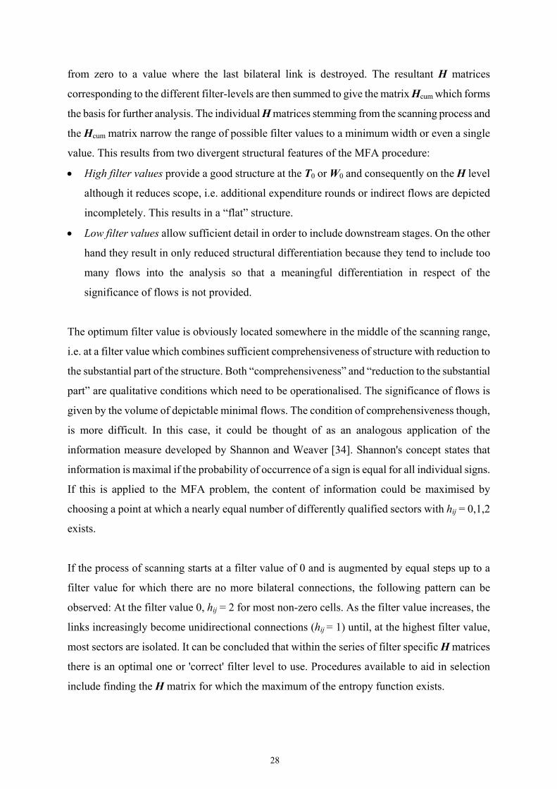
from zero to a value where the last bilateral link is destroyed. The resultant H matrices

corresponding to the different filter-levels are then summed to give the matrix Hcum which forms

the basis for further analysis. The individual H matrices stemming from the scanning process and

the Hcum matrix narrow the range of possible filter values to a minimum width or even a single

value. This results from two divergent structural features of the MFA procedure:

• High filter values provide a good structure at the T0 or W0 and consequently on the H level

although it reduces scope, i.e. additional expenditure rounds or indirect flows are depicted

incompletely. This results in a “flat” structure.

• Low filter values allow sufficient detail in order to include downstream stages. On the other

hand they result in only reduced structural differentiation because they tend to include too

many flows into the analysis so that a meaningful differentiation in respect of the

significance of flows is not provided.

The optimum filter value is obviously located somewhere in the middle of the scanning range,

i.e. at a filter value which combines sufficient comprehensiveness of structure with reduction to

the substantial part of the structure. Both “comprehensiveness” and “reduction to the substantial

part” are qualitative conditions which need to be operationalised. The significance of flows is

given by the volume of depictable minimal flows. The condition of comprehensiveness though,

is more difficult. In this case, it could be thought of as an analogous application of the

information measure developed by Shannon and Weaver [34]. Shannon's concept states that

information is maximal if the probability of occurrence of a sign is equal for all individual signs.

If this is applied to the MFA problem, the content of information could be maximised by

choosing a point at which a nearly equal number of differently qualified sectors with hij = 0,1,2

exists.

If the process of scanning starts at a filter value of 0 and is augmented by equal steps up to a

filter value for which there are no more bilateral connections, the following pattern can be

observed: At the filter value 0, hij = 2 for most non-zero cells. As the filter value increases, the

links increasingly become unidirectional connections (hij = 1) until, at the highest filter value,

most sectors are isolated. It can be concluded that within the series of filter specific H matrices

there is an optimal one or 'correct' filter level to use. Procedures available to aid in selection

include finding the H matrix for which the maximum of the entropy function exists.

29

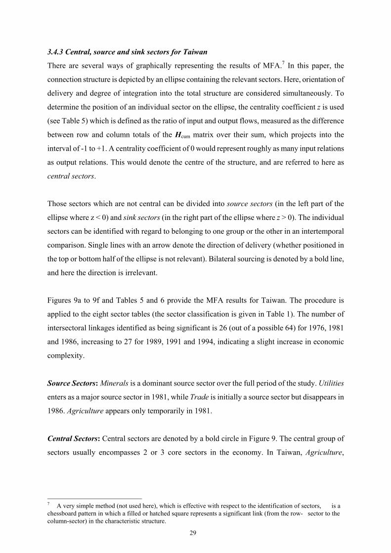
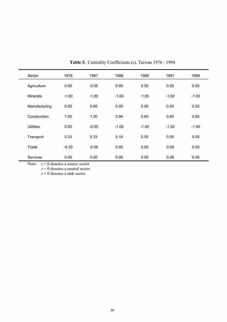
3.4.3 Central, source and sink sectors for Taiwan

There are several ways of graphically representing the results of MFA.7 In this paper, the

connection structure is depicted by an ellipse containing the relevant sectors. Here, orientation of

delivery and degree of integration into the total structure are considered simultaneously. To

determine the position of an individual sector on the ellipse, the centrality coefficient z is used

(see Table 5) which is defined as the ratio of input and output flows, measured as the difference

between row and column totals of the Hcum matrix over their sum, which projects into the

interval of -1 to +1. A centrality coefficient of 0 would represent roughly as many input relations

as output relations. This would denote the centre of the structure, and are referred to here as

central sectors.

Those sectors which are not central can be divided into source sectors (in the left part of the

ellipse where z < 0) and sink sectors (in the right part of the ellipse where z > 0). The individual

sectors can be identified with regard to belonging to one group or the other in an intertemporal

comparison. Single lines with an arrow denote the direction of delivery (whether positioned in

the top or bottom half of the ellipse is not relevant). Bilateral sourcing is denoted by a bold line,

and here the direction is irrelevant.

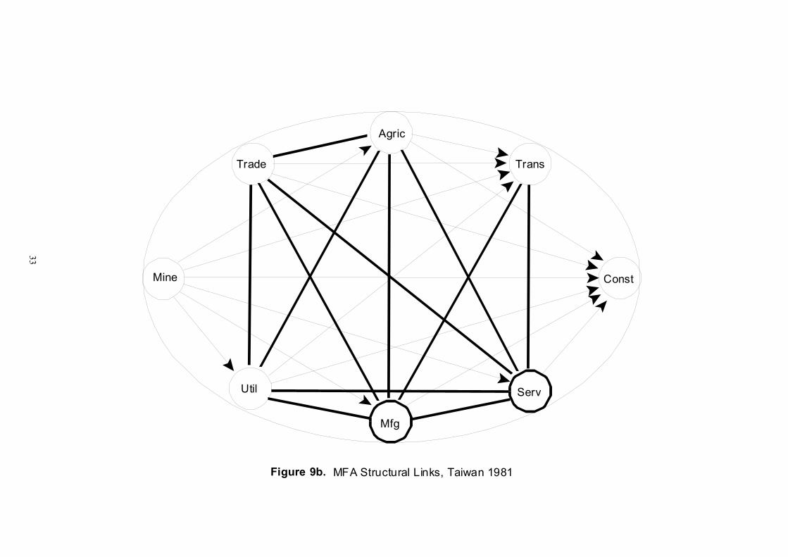
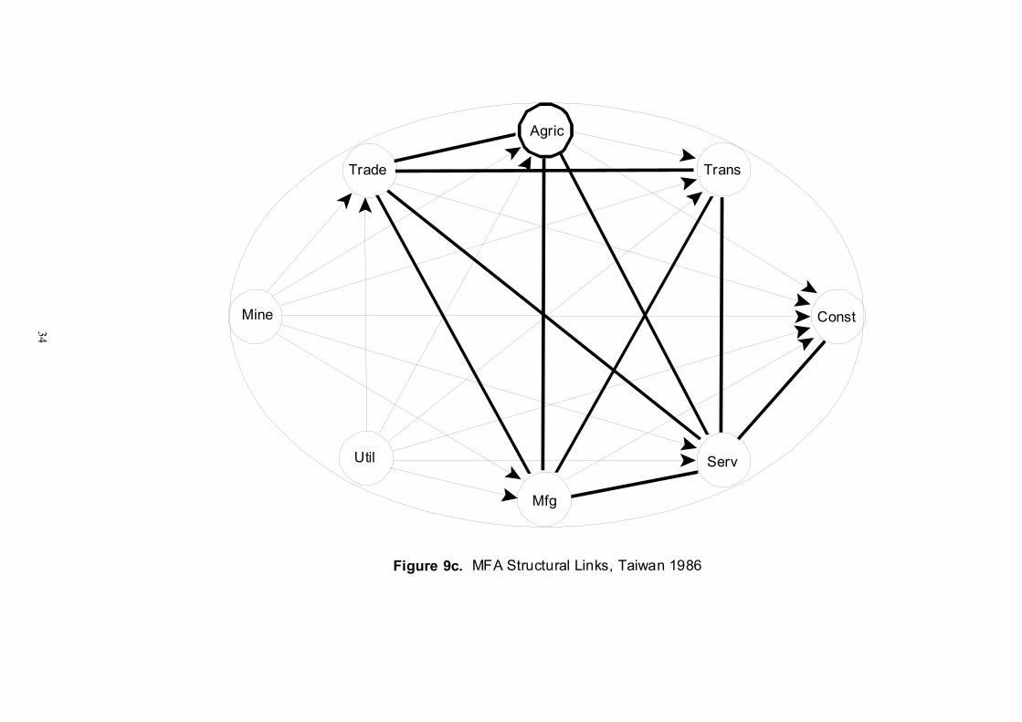
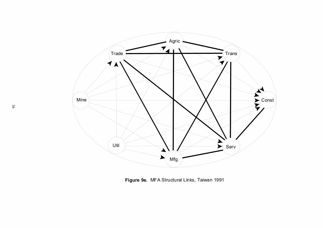
Figures 9a to 9f and Tables 5 and 6 provide the MFA results for Taiwan. The procedure is

applied to the eight sector tables (the sector classification is given in Table 1). The number of

intersectoral linkages identified as being significant is 26 (out of a possible 64) for 1976, 1981

and 1986, increasing to 27 for 1989, 1991 and 1994, indicating a slight increase in economic

complexity.

Source Sectors: Minerals is a dominant source sector over the full period of the study. Utilities

enters as a major source sector in 1981, while Trade is initially a source sector but disappears in

1986. Agriculture appears only temporarily in 1981.

Central Sectors: Central sectors are denoted by a bold circle in Figure 9. The central group of

sectors usually encompasses 2 or 3 core sectors in the economy. In Taiwan, Agriculture,

7 A very simple method (not used here), which is effective with respect to the identification of sectors, is a chessboard pattern in which a filled or hatched square represents a significant link (from the row- sector to the column-sector) in the characteristic structure.

30

Table 5. Centrality Coefficients (z), Taiwan 1976 - 1994 Sector

1976

1981

1986

1989

1991

1994

Agriculture

0.00

-0.05

0.00

0.05

0.05

0.05

Minerals

-1.00

-1.00

-1.00

-1.00

-1.00

-1.00

Manufacturing

0.00

0.00

0.05

0.05

0.05

0.05

Construction

1.00

1.00

0.56

0.60

0.60

0.60

Utilities

0.00

-0.05

-1.00

-1.00

-1.00

-1.00

Transport

0.33

0.33

0.18

0.05

0.05

0.05

Trade

-0.33

-0.05

0.05

0.05

0.05

0.05

Services

0.00

0.00

0.08

0.08

0.08

0.08

Note: z < 0 denotes a source sector z = 0 denotes a neutral sector z > 0 denotes a sink sector

31

Table 6. Synoptic Table of Sectoral Changes, Taiwan 1976 - 1994

Year

Source Sectors

Central Sectors

Sink Sectors

Number Unidirectional

Number Bilateral

1976

Minerals Trade

Agriculture Manufacturing Utilities Services

Construction Transport

16

10

1981

Agriculture Minerals Utilities Trade

Manufacturing Services

Construction Transport

14

12

1986

Minerals Utilities

Agriculture

Manufacturing Construction Transport Trade Services

16

10

1989

Minerals Utilities

Agriculture Manufacturing Construction Transport Trade Services

16

11

1991

Minerals Utilities

Agriculture Manufacturing Construction Transport Trade Services

16

11

1994

Minerals Utilities

Agriculture Manufacturing Construction Transport Trade Services

16

11

32

Mine

Trade

Agric

Trans

Const

Serv

Mfg

Util

Figure 9a. MFA Structural Links, Taiwan 1976

33

Mine

Trade

Agric

Trans

Const

Serv

Mfg

Util

Figure 9b. MFA Structural Links, Taiwan 1981

34

Mine

Trade

Agric

Trans

Const

Serv

Mfg

Util

Figure 9c. MFA Structural Links, Taiwan 1986

35

Mine

Trade

Agric

Trans

Const

Serv

Mfg

Util

Figure 9d. MFA Structural Links, Taiwan 1989

36

Mine

Trade

Agric

Trans

Const

Serv

Mfg

Util

Figure 9e. MFA Structural Links, Taiwan 1991

37 Mine

Trade

Agric

Trans

Const

Serv

Mfg

Util

Figure 9f. MFA Structural Links, Taiwan 1994

38

Manufacturing, Utilities and Services are initially classified as central sectors in 1976, but

Agriculture and Utilities drop out by 1981. By 1989 there are no central sectors left.

Sink Sectors: Initially, in 1976 and 1981, only Construction and Transport were identified

as sink sectors. Since then, there has been a progressive shift of all sectors except Minerals

and Utilities into the sink category. This again reinforces the notion of a weakening of the

intersectoral core, with no central sectors of substance to act as intermediaries and a

predominance of flows from Minerals and Utilities to the other sectors. Whilst there are

bilateral trade links with Trade, Agriculture, Manufacturing, Transport and Services, the

flows are predominately out rather than in.

3.4.4 Bilateral links between sectors

Bilateral links denote connections where sector i is both a source and sink sector for goods

and services to/from sector j to the extent that both deliveries are above the MFA-filter

level. This is due to the fact that both input coefficients aij and aji are considered high

compared to other sectoral links. As a consequence we could view both sectors i and j as a

growth dipol, since if one sector enhances its production (for whatever reason) this will

stimulate the other sector which in turn will result in higher demand for products from the

first sector. Thus sectors i and j form a growth core of the economy which in principle can

even be linked to a (bilateral) chain, star or triangle.

In Taiwan, bilateral connections initially revolve around the Agriculture-Utilities-

Manufacturing-Services group of sectors with Trade and Transport linked to a lesser

degree. Over time, Trade and Transport become more important as they occupy a central

position between the source and sink sectors. Utilities, on the other hand, loses its status as

an intermediary and becomes a pure source sector by 1986.

The MFA clearly shows that Taiwan has experienced structural shifts over the sample

period. For example, we can clearly see how Transport and Trade have emerged as

significant nodes and how Utilities has diminished in standing from being a part of 4

growth diapoles to a simple source sector. This would seem to indicate a gradual and

progressive shift towards a developed market economy, where economic coordination

occurs, to an increasing extent, through market intermediation. This also coincides with a

39

slowing-down of Taiwan’s economic growth, associated with a rapid appreciation of the

currency, rising real wages and declining exports (Wang [40]). Since the mid-1980s there

has been a rapid decline in the more labour-intensive industries as Taiwanese capital started

to move offshore, to mainland China and other South-East Asian economies with lower

labour costs (Amsden and Chu, [3]; Lin [26]).

4. SUMMARY AND CONCLUSION

The analysis confirms that there has been a shift in economic structure of the Taiwanese

economy. Firstly, there has been a pronounced shift in emphasis from primary activities to

secondary and tertiary activities. This has resulted in a more dichotomous structure

emerging in the sense that sectors can be identified as belonging predominately to either a

source or sink category. For example, Minerals has dominant forward linkages (i.e. is a

source sector), as demonstrated by all three techniques used in this paper (linkage, key

sector and minimal flow analyses), whereas Construction is similarly shown to have

dominant backward linkages (i.e. is a sink sector). Even the demand for manufactures has

decreased, shifting Manufacturing out of the central category into the sink category. This

has been associated with an increase in import reliance.

Secondly, it can be clearly seen from both the key sector analysis and minimal flow

analysis that the Taiwan economy reached a peak in terms of intersectoral complexity in

1981 before going into decline. This may be a direct consequence of the shifts in sectoral

emphasis noted above, as service industries require less physical inputs. This phenomenon

is not unique and may be associated with the movement of more labour intensive,

intermediate industries to low-wage countries, especially China, as part of the globalization

process. As trade barriers fall and ‘microeconomic’ reform policies bite, there is increased

specialisation and both vertical and horizontal integration of industry structures.

Government agencies no longer feel the need to support inefficient industries, with

consequent shifts in economic structure towards perceived industries with comparative

advantage and increased import reliance for other commodities.

40

REFERENCES

1. K. Abe. Japanese Direct Investment in the USA: Direct Investment, Hollowing-Out

and Deindustrialization. In Economic, industrial and managerial coordination

between Japan and the USA, pp. 27-59. St. Martin’s Press, New York; Macmillan

Press, London (1992).

2. J.M. Albala-Bertrand. Industrial Interdependence Change in Chile: 1960-90 a

comparison with Taiwan and South Korea. International Review of Applied

Economics. 13, 161-191 (1999).

3. A. Amsden and W-W. Chu. Upscaling: Recasting Old Theories to Suit Late

Industrializers. In Taiwan in the Global Economy (Edited by P.C.Y. Chow), pp. 23-

38. Praeger Publishers, USA (2002).

4. B. Andreosso-O’Callaghan and G. Yue. An Analysis of Structural Change in China

Using Biproportional Methods. Economic Systems Research. 12, 99-110 (2000).

5. R.G. Busacker and Th.L. Saaty. Endliche Graphen und Netzwerke. Oldenbourg,

München: Wien (1968).

6. R. Bon. Qualitative Input-Output Analysis. In Frontiers of Input-Output Analysis

(Edited by R.E. Miller, K.R. Polenske and A.Z. Rose), pp. 222-231 Oxford

University Press, Oxford (1989).

7. R.P.C. Brown and K. Hooper. Migration and the Nontradables Sectors: Evidence

From Taiwan. Paper presented at Taipei International Conference on Labour Market

Transformation and Labour Migration in East Asia, 21-23 June 1999, Institute of

Economics, Academia Sinica, Taipei (1999).

8. A.P. Carter. Changes in Input-Output Structure since 1972. Data Resources

Interindustry Review. 1, 11-17 (1980).

9. T.S. Chen. A Study on the structural changes in Taiwan’s industries: a rowscaler

method. Master’s Thesis, National Chung Cheng University (unpublished, in

Chinese).

10. H. Chenery. Patterns of Industrial Growth. American Economic Review. 50, 624–54

(1960).

11. H. Chenery. The Use of Interindustry Analysis in Development Programming. In

Structural Interdependence and Economic Development (Edited by T. Barna),

Macmillan, London (1961).

41

12. H.B. Chenery and M. Syrquin. Patterns of Development, 1950-1970. Oxford

University Press, London: (1975).

13. H.B. Chenery and T. Watanabe. International Comparisons of the Structure of

Production. Econometrica. 26, 487-521 (1958).

14. G. Chow and A-I. Lin. Accounting for Economic Growth in Taiwan and Mainland

China: A Comparative Analysis. Journal of Comparative Economics. 30, 507-530

(2002).

15. P.C.Y Chow. From Dependency to Interdependency: Taiwan’s Development Path

toward a Newly Industrialized Country. In Taiwan in the Global Economy (Edited by

P.C.Y. Chow), pp. 241-278. Praeger Publishers, USA (2002).

16. C. Clark. The Conditions of Economic Progress. Macmillan, London: (1940).

17. K. Cowling and P.R. Tomlinson. The Japanese Crisis-A Case of Strategic Failure?

Economic Journal. 110, 358-381 (2000).

18. J. Deutsch and M Syrquin. Economic Development and the Structure of Production.

Economic Systems Research. 1, 447–464 (1989).

19. S.E. Feinberg and M.P. Keane. U.S.-Canada Trade Liberalization and MNC

Production Location. Review of Economics and Statistics. 83, 118-132 (2001).

20. S.J. Feldman and K. Palmer. Structural Change in the United States: Changing Input-

Output Coefficients. Business Economics. 20, 38–54 (1985).

21. A.G.B. Fisher. Production, Primary, Secondary and Tertiary. Economic Record. 15,

24-38 (1939).

22. G.J.D. Hewings, M. Sonis, J. Guo, P.R. Israilevich and G.R. Schindler. The

Hollowing-Out Process in the Chicago Economy, 1975-2010. Regional Economics

Applications Laboratory Discussion Paper 96-T-1, University of Illinois (1996).

23. A.O. Hirschmann. The Strategy of Economic Development. Yale University Press,

New Haven (1958).

24. Y. Li and J-L. Hu. Technical Efficiency and Location Choice of Small and Medium-

Sized Enterprises. Small Business Economics. 19, 1-12 (2002).

25. K-S. Liang and C-I.H. Liang. Exports and Employment in Taiwan. In Institutes of

Economics, Academia Sinica, Conference on Population and Economic Development

in Taiwan, pp. 192-246. Taipei (1976).

26. S.A.Y. Lin. Roles of Foreign Direct Investments in Taiwan’s Economic Growth. In

Taiwan in the Global Economy (Edited by P.C.Y. Chow), pp. 79-94. Praeger

42

Publishers, USA (2002).

27. R.E. Miller and P.D. Blair. Input-Output Analysis: Foundations and Extensions.

Prentice Hall, Englewood Cliffs (1985).

28. Okazaki the 'Hollowing Out' Phenomenon in Economic Development. Paper

presented to the Pacific Regional Science Conference, Singapore (1989).

29. Y. Okina and A. Kohsaka. Japanese Corporations and Industrial Upgrading: Beyond

Industrial Hollowing-Out. Japan Research Quarterly. 5, 45-91 (1996).

30. P.E. Robertson. Why the Tigers Roared: Capital Accumulation and the East Asian

Miracle. Pacific Economic Review. 7, 259-274 (2002).

31. P. Rasmussen. Studies in Intersectoral Relations. North-Holland, Amsterdam (1957).

32. H. Schnabl. The Evolution of Production Structures - Analysed by a Multi Layer

Procedure. Economic Systems Research. 6, 51-68 (1994).

33. H. Schnabl and H.W. Holub. Qualitative und Quantitative Aspekte der Input-Output

Analyse. Zeitschrift für die gesamte Staatswissenschaft. 135, 657-678 (1979).

34. C.E. Shannon and W. Weaver. The Mathematical Theory of Communication.

University of Illinois Press, Urbana (1949).

35. M. Sonis, G.J.D. Hewings and J. Guo. A New Image of Classical Key Sector

Analysis: Minimum Information Decomposition of the Leontief Inverse. Economic

Systems Research. 12, 401-423 (2000).

36. M. Syrquin. Patterns of Structural Change. In Handbook of Development Economics,

Volume I (Edited by H.B. Cherney and T.N. Srinivasan), Elsevier Science

Publishers, Amsterdam (1988).

37. M. Syrquin and H.B. Chenery. Patterns of Development 1950 to 1983. The World

Bank, Washington (1986).

38. E. Thorbecke and H. Wan. Taiwan’s Development Experience: Lessons on Roles of

Government and Market. Kluwer Academic Publishers, USA (1999).

39. C. Wang, J. Sun, and T. Chou. Sources of Economic Growth and Structural Change:

A Revised Approach. Journal of Development Economics. 38, 383–401 (1992).

40. E.C. Wang. A Multiplicative Decomposition Method to Identify the Sectoral

Changes in Various Developmental Stages: Taiwan, 1966-91. Economic Systems

Research. 8, 0953-5314 (1996).

41. E.C. Wang. Structural Change and Industrial Policy in Taiwan, 1966–91: An

Extended Input–Output Analysis. Asian Economic Journal. 11, 187-206 (1997).

43

42. G. West. Sensitivity and Key Sector Analysis in Input-Output Models. Australian

Economic Papers. 21, 365-378 (1982).

43. G. West. Structural Change in the Queensland Economy: An Interindustry Analysis.

Economic Analysis and Policy, 0, 27-51 (1999).

44. World Bank. The East Asian Miracle: Economic Growth and Public Policy. Oxford

University Press, New York (1993).

45. A. Young. Lessons from the East Asian NICs: A Contrarian View. European

Economic Review. 38, 964-973 (1994).