structural behavior of concrete shear keys in the nanchang ... · structural behavior of concrete...

Structural Behavior of Concrete Shear Keys in the

Nanchang Red Valley Immersed Tunnel

Thomas Mertens

Supervisors: Prof. Luc Taerwe, Prof. Yong Yuan

Master's dissertation submitted in order to obtain the academic degree of

Master of Science in Civil Engineering

Department of Structural Engineering

Chair: Prof. dr. ir. Luc Taerwe

Faculty of Engineering and Architecture

Academic year 2015-2016

2

Preface

This master's dissertation is the result of research performed at Tongji University in Shanghai,

P.R. China, and Ghent University, Belgium. The thesis document is for the largest part written at the

Geotechnical Department of Tongji University in Shanghai and on the construction site of the Red

Valley immersed tunnel in Nanchang. The subject of this dissertation fits in the context of ongoing

research at Tongji University about the structural behavior of the Jianxi Nanchang Red Valley

immersed tunnel.

I would like to thank Professor Yong Yuan and Professor Luc Taerwe for their support and

cooperation, both in China and in Belgium. My gratitude goes to Professor Haitao Yu for the

guidance and discussions in Shanghai. Also I would like to praise my colleagues and friends, Jian Hui

Luo and Yikang Cheng for a pleasant time together at the Tongji University Geotechnical

Department.

Finally, sincere gratitude goes to my parents and my girlfriend for their support and encouragement

during my complete study at Ghent University.

The financial support of the Chinese Government Ministry of Education in the form of a CSC-

scholarship is gratefully acknowledged.

The author gives permission to make this master dissertation available for consultation and to copy

parts of this master dissertation for personal use. In the case of any other use, the copyright terms

have to be respected, in particular with regard to the obligation to state expressly the source when

quoting results from this master dissertation.

June 2016

3

Abstract

The immersed tunnel technique is a common technique for crossing rivers, lakes and sea in the

People's Republic of China. Although historically most immersed tunnel construction occurred in

the Netherlands, the United States and Japan, the construction of immersed tunnels in China has

increased rapidly in the last decades. Currently the People's republic of China has no National

Standard design code for immersed tunnels and their design is often accompanied by numerical

studies and physical tests.

The focus of this dissertation is the behavior of the concrete shear keys of a physical scale model of

the Nanchang Red valley immersed tunnel under static loads. The Nanchang Red valley immersed

tunnel is under construction during the period in which this dissertation is written (2015-2016).

Because concrete shear keys are loaded most heavily when the immersed tunnel is loaded in the

lateral direction, the loading case that is of prior interest is lateral loading of the tunnel elements in

combination with the axial load of the tunnel elements that is inherent to immersed tunnels due to

their construction process.

The structural behavior of the joint of a scale model of the Nanchang Red Valley immersed tunnel is

assessed. Tests are conducted through numerical analysis, and can later be compared with results

from physical scale model testing. For both the numerical model and the physical test, a

geometrical scale of 1:5 is used relative to the real tunnel prototype. The overall dimensions of the

cross-section of both the numerical model and the physical scale model are 6 m × 1,66 m.

The numerical analysis is performed by using the finite element (FE) software package Abaqus. The

FE model is composed of the ends of 2 adjacent tunnel elements, and their mutual joint. Its purpose

is to predict the structural behavior of the joint under lateral loading that will occur in the physical

scale model test. The results of the numerical analysis can be useful in the design of the physical

scale model experiment. After the physical scale model tests, the numerical results can be verified

and numerical parameters can be calibrated further, so that numerical modeling of future

immersed tunnel projects can be performed more reliably.

4

Table of Contents

Preface...................................................................................................................................................... .. 2

Abstract..... .............................................................................................................................................. 3

Table of Contents ..................................................................................................................................... 4

List of Figures ........................................................................................................................................... 7

List of Tables .......................................................................................................................................... 10

List of Symbols ....................................................................................................................................... 12

I Introduction ......................................................................................................................... 14

1 Problem definition ................................................................................................................................. 14

2 Main research question ......................................................................................................................... 14

3 Sub-questions ........................................................................................................................................ 15

4 Objective ................................................................................................................................................ 15

5 Structure of the report .......................................................................................................................... 15

II Immersed tunneling .............................................................................................................. 16

1 Abstract ................................................................................................................................................. 16

2 Definition ............................................................................................................................................... 16

3 Comparison to other tunnel types ........................................................................................................ 17

4 Construction method ............................................................................................................................ 18

4.1 Overview of the construction process................................................................................................... 18

4.2 Immersed joints ..................................................................................................................................... 21

4.2.1 Structural configuration ...................................................................................................................... 21

4.2.2 Elements for watertightness ............................................................................................................... 23

4.2.3 Shear keys............................................................................................................................................ 26

III Design starting points ........................................................................................................... 28

1 Nanchang Red Valley tunnel.................................................................................................................. 28

2 Immersed joint shear key configuration ............................................................................................... 29

2.1 Tunnel geometry ................................................................................................................................... 29

2.1.1 Cross section ....................................................................................................................................... 29

2.1.2 Shear keys............................................................................................................................................ 30

2.1.3 Gina gasket and omega seal ................................................................................................................ 30

2.1.4 Length profile ...................................................................................................................................... 31

2.2 Axial load ............................................................................................................................................... 32

5

IV Numerical modeling of the Red Valley tunnel ........................................................................ 33

1 The Abaqus software package ............................................................................................................... 33

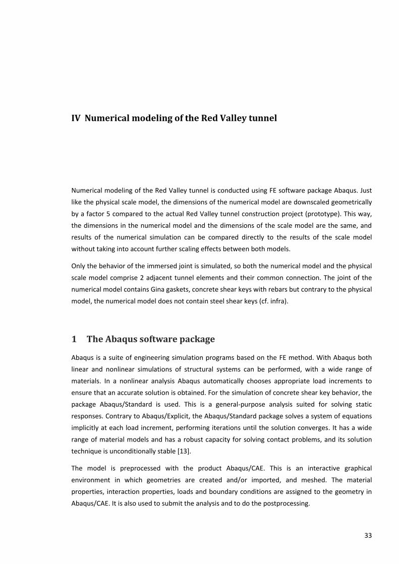
2 Model design ......................................................................................................................................... 34

2.1 Dimensional similitude .......................................................................................................................... 34

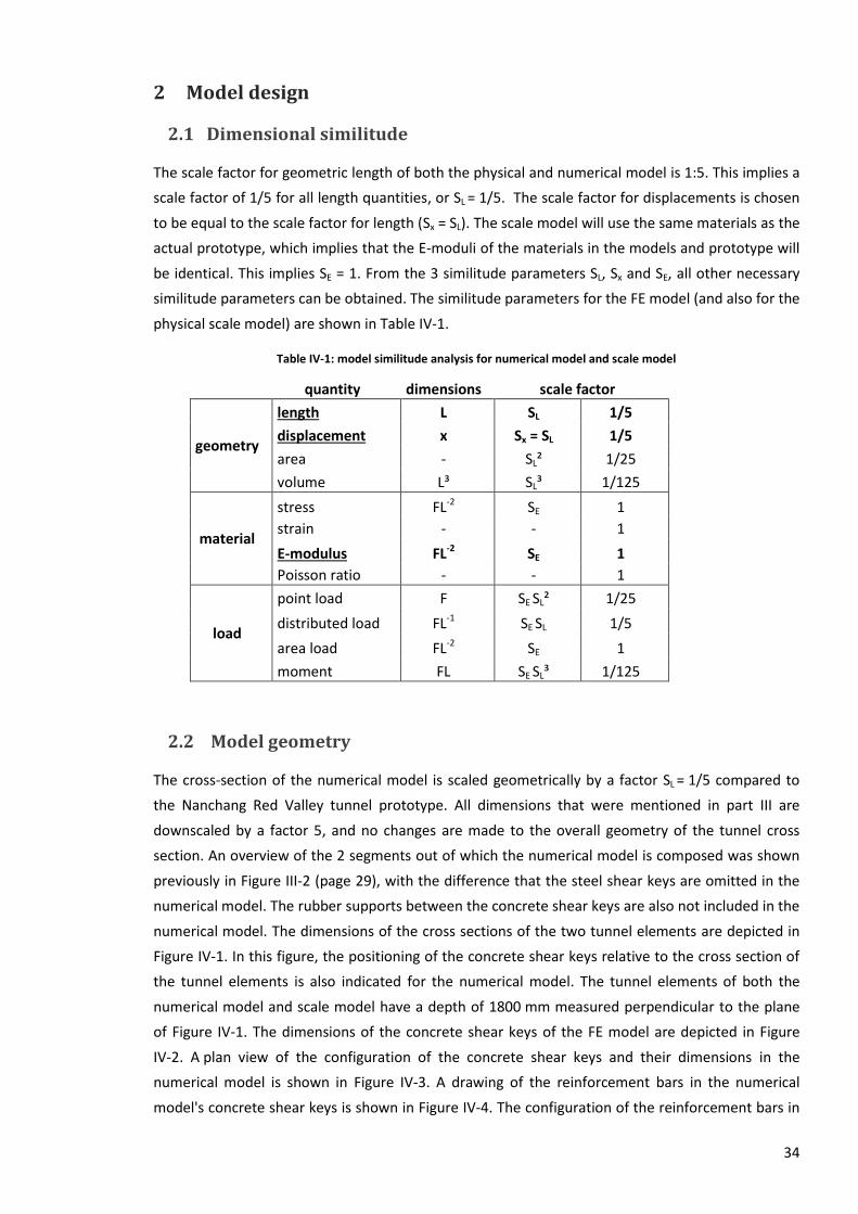
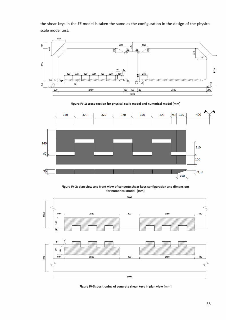
2.2 Model geometry .................................................................................................................................... 34

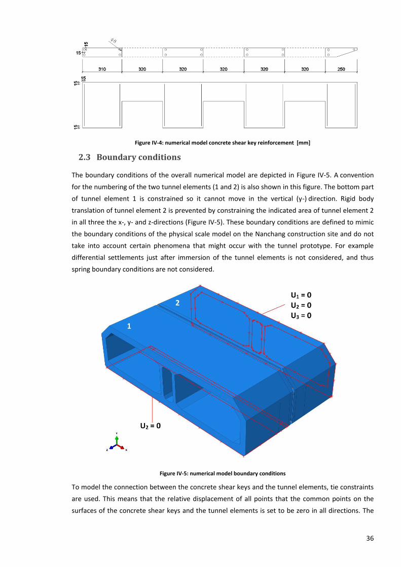
2.3 Boundary conditions .............................................................................................................................. 36

2.4 Loads ...................................................................................................................................................... 37

2.4.1 Considered loading case ...................................................................................................................... 37

2.4.2 Axial load on tunnel face .................................................................................................................... 38

2.4.3 Lateral loads on tunnel side ................................................................................................................ 38

3 Materials and interaction behavior ....................................................................................................... 39

3.1 Plain concrete material model .............................................................................................................. 39

3.1.1 Uniaxial loading ................................................................................................................................... 40

3.1.2 Multiaxial conditions ........................................................................................................................... 44

3.1.3 Yield condition ..................................................................................................................................... 45

3.1.4 Flow rule .............................................................................................................................................. 46

3.1.5 Viscoplastic regularization ................................................................................................................... 47

3.1.6 Summary ............................................................................................................................................. 48

3.2 Concrete shear key teeth interaction behavior .................................................................................... 48

3.3 Steel reinforcement ............................................................................................................................... 49

3.3.1 Steel material ...................................................................................................................................... 49

3.3.2 Defining reinforcement bars in Abaqus .............................................................................................. 49

3.4 Rubber material model .......................................................................................................................... 50

3.5 Rubber-concrete interaction behavior .................................................................................................. 51

4 Numerical test results............................................................................................................................ 51

4.1 Preliminary calculations ........................................................................................................................ 51

4.2 Load increments .................................................................................................................................... 51

4.3 Ultimate lateral load .............................................................................................................................. 53

4.4 Concrete shear key damage .................................................................................................................. 54

6

4.4.1 Occurrence of cracks in concrete shear keys ...................................................................................... 55

4.4.2 Joint stiffness degradation .................................................................................................................. 58

4.4.3 Crack directions ................................................................................................................................... 60

4.4.4 Summary ............................................................................................................................................. 60

4.5 Load distribution ................................................................................................................................... 63

4.5.1 Influence of steel shear keys ............................................................................................................... 63

4.5.2 Concrete shear keys reaction forces ................................................................................................... 64

4.5.3 Load distribution between Gina gasket and concrete shear keys ...................................................... 71

4.5.4 Relation between load distribution and concrete shear key damage ................................................ 72

4.5.5 Load distribution between the concrete shear key teeth ................................................................... 72

4.5.6 Load distribution between the concrete shear keys ........................................................................... 75

4.5.7 Consequences for physical scale model pressure gauges ................................................................... 78

4.5.8 Discussion of FE model load distribution ............................................................................................ 81

4.5.9 Proposal of simplified model for damage assessment ....................................................................... 83

4.5.10 Summary ............................................................................................................................................. 86

V Conclusions .......................................................................................................................... 88

VI References............................................................................................................................ 90

VII Addenda ............................................................................................................................... 92

7

List of Figures

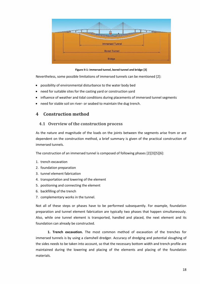
Figure II-1: immersed tunnel, bored tunnel and bridge [3]................................................................... 18

Figure II-2: casting basin in Nanchang, China ........................................................................................ 19

Figure II-3: production steps in casting basin of Nanchang project (November 2015) ......................... 20

Figure II-4: transportation of tunnel elements with survey towers using catamarans [3] ................... 20

Figure II-5: positioning adjacent elements and dewatering voids between bulkheads [5] .................. 21

Figure II-6: backfill material is laced besides and over the tunnel [3] .................................................. 21

Figure II-7: details and cross-section of the immersion joint of HZMB Tunnel [7] ............................... 22

Figure II-8: Structure of immersion joint with shear keys, Mexico [mm] [8] ....................................... 23

Figure II-9: Structure of immersion joint with shear keys, Japan [9] .................................................... 23

Figure II-10: different kind of waterstop gaskets [11] .......................................................................... 24

Figure II-11: components of immersion joint [2] .................................................................................. 24

Figure II-12: Mounting system for Gina seal in Nanchang project ........................................................ 25

Figure II-13: example of an expansion joint between 2 segments [mm] [10] ...................................... 25

Figure II-14: Rubber waterstops used to ensure watertightness between two casts in the Nanchang

project ................................................................................................................................................... 26

Figure II-15: provisions to attach vertical shear keys in Nanchang project .......................................... 27

Figure II-16: concrete shear key connection rebars in the Nanchang Red Valley immersed joint (side

view) [mm]............................................................................................................................................. 27

Figure III-1: overview of the Nanchang construction site ..................................................................... 28

Figure III-2: schematic overview of locations of shear keys on tunnel element ................................... 29

Figure III-3: cross-section of the Red Valley Tunnel [mm] .................................................................... 30

Figure III-4: plan view of concrete shear keys configuration and dimensions [mm] ........................... 30

Figure III-5: Gina gasket, omega seal (l) and Gina gasket dimensions (r) [mm] ................................... 31

Figure III-6: configuration of Gina seal on face of tunnel element [mm] ............................................. 31

Figure III-7: length profile of Red Valley tunnel [m] .............................................................................. 31

Figure IV-1: cross-section for physical scale model and numerical model [mm] .................................. 35

Figure IV-2: plan view and front view of concrete shear keys configuration and dimensions for

numerical model [mm] ......................................................................................................................... 35

8

Figure IV-3: positioning of concrete shear keys in plan view [mm] ...................................................... 35

Figure IV-4: numerical model concrete shear key reinforcement [mm] .............................................. 36

Figure IV-5: numerical model boundary conditions .............................................................................. 36

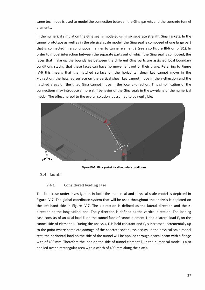
Figure IV-6: Gina gasket local boundary conditions .............................................................................. 37

Figure IV-7: axial and lateral loading case on the tunnel model and global coordinate system........... 38

Figure IV-8: concrete behavior in uniaxial tension [14] ........................................................................ 41

Figure IV-9: concrete behavior in uniaxial compression [14] ................................................................ 41

Figure IV-10: uniaxial strains in function of inelastic stresses ......................................................... 42

Figure IV-11: damage parameters as functions of the cracking strain and inelastic strain in numerical

model ..................................................................................................................................................... 44

Figure IV-12: Contact pressure-clearance relationship for “hard” contact [20] ................................... 48

Figure IV-13: linear penalty method [21] .............................................................................................. 48

Figure IV-14: steel plastic behavior definition in numerical model....................................................... 49

Figure IV-15: axial loads in numerical model......................................................................................... 52

Figure IV-16: lateral load in numerical model ....................................................................................... 53

Figure IV-17: tunnel element 1 concrete shear keys load-displacement curve .................................... 53

Figure IV-18: concrete shear key indication convention ....................................................................... 55

Figure IV-19: maximal principal plastic strain [-] at Fs = 79 kN .............................................................. 56

Figure IV-20: tensile equivalent plastic strain [-] at Fs = 79 kN ...................................................... 56

Figure IV-21: damage parameter dt [-] at Fs = 79 kN ............................................................................. 57

Figure IV-22: concrete tensile damage parameter [-] at lateral loads of 100 kN, 122 kN and 146 kN . 58

Figure IV-23: concrete tensile damage parameter [-] at Fs = 250 kN .................................................... 59

Figure IV-24: absolute displacement in lateral (x-)direction [mm] at Fs = 300 kN [mm]....................... 59

Figure IV-25: maximum Mises stress of rebars in all concrete shear key teeth .................................... 60

Figure IV-26: direction and magnitude of maximum principal strain [-] at Fs = 79 kN .......................... 61

Figure IV-27: direction and magnitude of maximum principal strain [-] ............................................... 62

Figure IV-28: load transfer members in immersed joint ....................................................................... 64

Figure IV-29: absolute displacement in y-direction [mm] of tunnel element 1 (a) and element 2 (b) . 64

Figure IV-30: contact pressures on side of concrete shear keys [N/mm²] ............................................ 65

9

Figure IV-31: rubber supports in physical scale model ......................................................................... 65

Figure IV-32: numerical result of contact pressure on shear key 1.2 .................................................... 67

Figure IV-33: reaction forces on teeth of concrete shear key 1 (Fs = 100 kN) ....................................... 68

Figure IV-34: reaction forces on teeth of concrete shear key 2 (Fs = 100 kN) ....................................... 69

Figure IV-35: tunnel elements absolute displacement in z-direction [mm] under lateral load of

100 kN .................................................................................................................................................... 70

Figure IV-36: angular rotation [rad] of tunnel element 1 relative to tunnel element 2 ....................... 70

Figure IV-37: fraction of lateral load taken up by Gina gaskets ............................................................ 71

Figure IV-38: fraction of Fs taken up by concrete shear key parts for varying Fs .................................. 73

Figure IV-39: tooth of shear key 2 linear regression ............................................................................. 74

Figure IV-40: tooth of shear key 1 linear regression ............................................................................. 75

Figure IV-41: fraction of Fs taken up by concrete shear keys and Gina for varying Fs ........................... 76

Figure IV-42: fraction of Fs taken up by concrete shear keys and Gina for varying Fs, linear fit ........... 77

Figure IV-43: regression model for shear key 1 and shear key 2 .......................................................... 78

Figure IV-44: theoretical triangular load distribution on shear key 2 ................................................... 79

Figure IV-45: simplified numerical model ............................................................................................. 84

Figure IV-46: simplified of lateral loading on concrete shear key teeth (proposal) .............................. 84

Figure IV-47: concrete tensile damage parameter dt [-] at varying lateral loads, simplified numerical

model ..................................................................................................................................................... 86

Figure VII-1: dimensionless material constants for concrete tensile constitutive relation [18] ........... 94

Figure VII-2: uniaxial stress-strain relation of C40 concrete under tension .......................................... 95

10

List of Tables

Table IV-1: model similitude analysis for numerical model and scale model ....................................... 34

Table IV-2: plain concrete material parameters .................................................................................... 39

Table IV-3: steel reinforcement material parameters ........................................................................... 39

Table IV-4: inelastic stresses as functions of the cracking strain and inelastic strain in numerical

model ..................................................................................................................................................... 42

Table IV-5: damage parameters as tabular functions of the cracking strain and inelastic strain in

numerical model .................................................................................................................................... 44

Table IV-6: Numerical model concrete plastic-damage parameters ..................................................... 48

Table IV-7: inelastic strain in function of stress beyond elastic region ................................................. 49

Table IV-8: numerical model rubber material parameters ................................................................... 50

Table IV-9: area of tunnel face and tunnel side of numerical model .................................................... 51

Table IV-10: loading cases ..................................................................................................................... 52

Table IV-11: estimated location, load and direction of crack initiation of concrete shear keys ........... 61

Table IV-12: reaction forces on concrete shear keys and Gina under lateral load of 100 kN ............... 69

Table IV-13: fraction of Fs taken up by concrete shear keys and Gina for varying Fs ............................ 72

Table IV-14: linear regression analysis on shear key teeth reaction forces .......................................... 73

Table IV-15: linear regression analysis on shear key reaction forces .................................................... 76

Table IV-16: calculated average contact pressures on concrete shear key teeth [N/mm²] .................. 79

Table IV-17: estimated maximum contact pressures on concrete shear key teeth based on FE results

[N/mm²] ................................................................................................................................................. 80

Table IV-18 location, load and direction of crack initiation of concrete shear keys (alternative

method) ................................................................................................................................................. 85

Table VII-1: uniaxial elastic strains in function of inelastic stresses ...................................................... 96

Table VII-2: reaction forces on concrete shear keys and Gina under lateral load of 10 kN ................ 101

Table VII-3: reaction forces on concrete shear keys and Gina under lateral load of 58 kN ................ 101

Table VII-4: reaction forces on concrete shear keys and Gina under lateral load of 100 kN .............. 101




11



Table VII-10: reaction forces on concrete shear keys and Gina under lateral load of 280 kN ............ 103

12

List of Symbols

Latin symbols

A area

C10 first empirical shear constant in Mooney-Rivlin model

C01 second empirical shear constant in Mooney-Rivlin model

d scalar degradation variable

D undamaged elasticity matrix

D1 compressibility constant in Mooney-Rivlin model

E modulus of elasticity

F load

F() yield function

f strength

G flow potential

Hr material hardness

I1 first invariant of Green

I2 second invariant of Green

K stiffness

p contact pressure

effective hydrostatic pressure

Mises equivalent effective stress

r principal stress weight factor

R² coefficient of determination

S scale factor

deviatory part of effective stress tensor

t time

W strain energy potential

x horizontal, lateral direction

y vertical direction

y fraction of lateral load

z horizontal, axial direction

Greek symbols

α significance level

α angular rotation

α concrete dimensionless material constant (1)

β concrete yield condition parameter

γ concrete dimensionless material constant (2)

ε strain

ϵ element of a (numerical) set

ϵ flow rule eccentricity

η dimensionless stress of concrete

μ viscosity parameter

μ coefficient of friction

τ shear stress

σ normal stress

φ bar diameter

ψ flow rule dilatation angle

13

ξ dimensionless strain of concrete

Subscripts

c compression

E stiffness

f axial (load, on tunnel face)

in initial

l lateral (stiffness)

L length

s lateral (load, on tunnel side)

t tension

u ultimate value

v viscous

x displacement

y yield

0 initial

Superscripts el elastic pl plastic

Abbreviations, acronyms and units

CI confidence interval

cm centimeter

FE finite element

HWL high water level

HPC high performance concrete

HZMB Hong Kong-Zhuhai-Macao bridge tunnel

kN kilonewton

LWL low water level

m meter

max maximum

min minimum

mm millimeter

N Newton

MPa megapascal

rad radians

sec seconds

14

I Introduction

1 Problem definition

The immersed tunneling technique is a common technique for crossing rivers, lakes and sea in the

People's Republic of China. Currently the People's republic of China has no National Standard design

code for immersed tunnels and their design is often accompanied by numerical studies and physical

tests. An immersed tunnels is composed of prefabricated elements that are placed in trenches that

have been dredged in river or sea bottoms, and that are afterwards interconnected. The joints that

connect the adjacent tunnel elements are considered to be the weakest elements in the whole

tunnel.

To assess the behavior of the joint of the Nanchang Red Valley immersed tunnel, a physical scale

model with a geometric scale of 1:5 will be built on the Red Valley tunnel construction site and will

be loaded laterally until failure. Two quasi-static loading cases will be considered: combined axial

and vertical loading, and combined axial and lateral loading. This dissertation focuses on the latter

loading case.

Prior to testing of the physical scale model, its behavior is difficult to predict. Nevertheless decisions

have to be made concerning the design of the scale model and the test setup. Prior to the test, the

ultimate load of the physical scale model is unknown, so that it is not known which loading

configuration is best suited for the scale model test. Also, the location and specifications of the

strain gauges and pressure sensors depend on the damage phenomena that are expected to occur

during the physical scale model test as well as the pressures that will occur locally.

A numerical (FE) model is used to predict the behavior of the 1:5 physical scale model. The following

research questions are formulated.

2 Main research question

What is the structural behavior of the concrete shear keys in a 1:5 physical scale model of the

Nanchang Red Valley tunnel under static lateral loading?

15

3 Sub-questions

1. How can the materials and the structural configuration of the joint of an immersed tunnel be

modeled using FE software?

2. How can we predict the ultimate lateral load that can be applied to the 1:5 physical scale model

of the Red Valley immersed tunnel using FE simulation;

3. How can the damage phenomena that will occur in the concrete shear keys in the 1:5 physical

scale model of the Red Valley immersed tunnel be predicted;

4. How can the distribution of the externally applied lateral loads over the structural elements in

the immersed joints be assessed?

4 Objective

The objective of this dissertation is to construct a numerical model with which the structural

behavior that will occur in an physical scale model of the Nanchang Red Valley immersed tunnel can

be predicted. The aim of the numerical modeling is to provide useful information for the set-up of

the physical scale model and to predict certain aspects of the response of the scale model. In a later

stage the results from the physical model can provide useful feedback to further enhance initial

numerical models, so that future numerical analyses of immersed tunnel joints can be performed

more accurately.

5 Structure of the report

Part I of the report contains general information on this master's dissertation. Part II of this report is

an introduction on immersed tunneling, their construction technique and on immersed joints. In

part III the Nanchang Red Valley project is introduced. The design of this project is the starting point

for the numerical and physical simulations. Part IV explains the design of the numerical model, and

contains the results from the numerical tests. Part V contains final conclusions.

16

II Immersed tunneling

1 Abstract

An immersed tunnels is composed of prefabricated elements. The elements are placed in trenches

that have been dredged in river or sea bottoms, and are afterwards interconnected. The joints that

connect the adjacent tunnel elements are considered to be the weakest elements in the whole

tunnel. Whereas steel immersed tunnels have a structural system that is composed of stiffened

structural steel plates working compositely with interior concrete, concrete tunnels have passively

reinforced and/or pre-stressed concrete as the main structural material [1][2].

In the following paragraphs, an overview of selected literature concerning immersed tunneling is

provided. As there is not many literature available on the structural behavior of the joints, the focus

is primarily on the tunnel structure and on the construction method of immersed tunnels.

2 Definition

An immersed tunnel is a passageway below water level, that consists of one or more prefabricated

elements that are floated to the site, installed one by one, and interconnected under water. An

immersed tunnel is generally installed in a trench that has been dredged previously at the bottom

of a river, lake or sea, and connects terminal structures that are located on land.

The space between the trench bottom and the soffit of the tunnel can be a gravel or a sand bed.

After placement of the elements, the tunnel trench is backfilled and the completed tunnel is usually

covered with a protective layer of stone/rock over the roof [1][3].

Two main types of immersed tunnels exist, namely steel and concrete immersed tunnels. The

structural system of steel tunnels is made of stiffened structural steel plates, working compositely

with interior concrete. Concrete tunnels on the other hand, have pre-stressed and/or passively

reinforced concrete as the main structural material [1][2].

17

3 Comparison to other tunnel types

Currently, 3 types of tunnels exist, namely cut-and-cover tunnels, subsurface excavation tunnels

and immersed tunnels. The possibility of a fourth type of tunnel, i.e. floating tunnel, is being

examined but has currently not been built for human transportation [4].

Cut-and-cover tunnels, also called surface tunnels or open excavation tunnels, are built by

excavating a trench and constructing the tunnel structure or placing the prefabricated elements in

the trench. After the completion of the underground structure, the trench is backfilled with soil.

Cut-and-cover tunnels are shallow tunnels, typically less than 30 meters below ground level [2].

Subsurface excavation tunneling comprises two different tunneling techniques: mechanical

tunneling and conventional tunneling. In mechanical tunneling, the excavation is done by using full-

face tunnel boring machines (TBMs). Conventional tunneling uses small drill holes in which

explosives are placed, together with mechanical excavators (but not full-face TBM's) [2].

Contrary to cut-and cover tunnels, an immersed tunnel only functions to cross rivers, lakes and sea.

Unlike subsurface excavation tunnels, they rest on the river- or seabed. The immersed tunnel's

prefabricated elements are placed in trenches that have been dredged at the river or sea bottom,

and that are interconnected after placement. The joints that connect the adjacent tunnel elements

are considered to be the weakest elements in the whole tunnel [1].

Compared to cut-and-cover tunnels and subsurface excavation tunnels, immersed tunnels have

some specific advantages [2][3]:

possibility of non-circular cross-section and versatility of cross-section geometry

tunnel construction is possible with ground conditions that are not feasible for subsurface

excavation, such as soft alluvial deposits in for example river estuaries.

prefabricated construction in dry docks under normal working conditions promotes construction

quality

placement of tunnel elements on the bed of the waterway yields more shallow construction, and

thus shorter tunnel approaches (Figure II-1)

construction, placement and further detailing of different parts of the tunnel can happen

simultaneously

fewer in-situ joints.

These advantages can make immersed tunnel more viable for river or sea passages than other

tunneling methods concerning total project cost, operational aspects and technical feasibility.

18

Figure II-1: immersed tunnel, bored tunnel and bridge [3]

Nevertheless, some possible limitations of immersed tunnels can be mentioned [2]:

possibility of environmental disturbance to the water body bed

need for suitable sites for the casting yard or construction yard

influence of weather and tidal conditions during placements of immersed tunnel segments

need for stable soil on river- or seabed to maintain the dug trench.

4 Construction method

4.1 Overview of the construction process

As the nature and magnitude of the loads on the joints between the segments arise from or are

dependent on the construction method, a brief summary is given of the practical construction of

immersed tunnels.

The construction of an immersed tunnel is composed of following phases [2][3][5][6]:

1. trench excavation

2. foundation preparation

3. tunnel element fabrication

4. transportation and lowering of the element

5. positioning and connecting the element

6. backfilling of the trench

7. complementary works in the tunnel.

Not all of these steps or phases have to be performed subsequently. For example, foundation

preparation and tunnel element fabrication are typically two phases that happen simultaneously.

Also, while one tunnel element is transported, handled and placed, the next element and its

foundation can already be constructed.

1. Trench excavation. The most common method of excavation of the trenches for

immersed tunnels is by using a clamshell dredger. Accuracy of dredging and potential sloughing of

the sides needs to be taken into account, so that the necessary bottom width and trench profile are

maintained during the lowering and placing of the elements and placing of the foundation

materials.

19

The purpose of the excavation is to make space for the prefabricated tunnel body, the sand or

gravel foundation under the body and the protective backfill at the sides and the top of the tunnel.

2. Foundation preparation. Foundation treatment methods depend on local geologic

conditions. Pile foundations are used when differential settlements are feared due to varying

stiffness of the subsoil along the tunnel length, due to vibrations of the tunnel or due to serious

sediment inclusion in areas with extreme soft subsoil.

An alternative to constructing a pile foundation is to use sand jetting. In this technique, the tunnel

elements are placed directly on the sea- or riverbed and sand is dispersed horizontally in clearance

areas between the tunnel elements and the subsoil through openings in the bottom slab.

A third alternative is the construction of a gravel bed prior to placement of the element, with or

without the use of special grout. This third technique gives a higher foundation stiffness than the

sand jetting technique, but requires more accuracy during the construction of the foundation layer.

The usage of sand as foundation material is not advised in areas with seismic activities, as the

loading capacity of the foundation may be diminished due to liquefaction of the sand.

3. Tunnel element fabrication. Tunnel elements are fabricated off-site, usually in dry docks

or in specially constructed casting basins. Tunnel elements are normally between 80 m and 150 m

long, and can consist of several interconnected segments. The length of segments usually varies

between 15 and 25 m. Prior to transportation, the ends of each element are closed by bulkheads to

make the element watertight. The bulkheads are set back a nominal distance from the end of the

element, resulting in a small space at the ends of the adjoining sections that is filled with water

when elements are interconnected. This space requires dewatering after the connection with the

previously installed element is made.

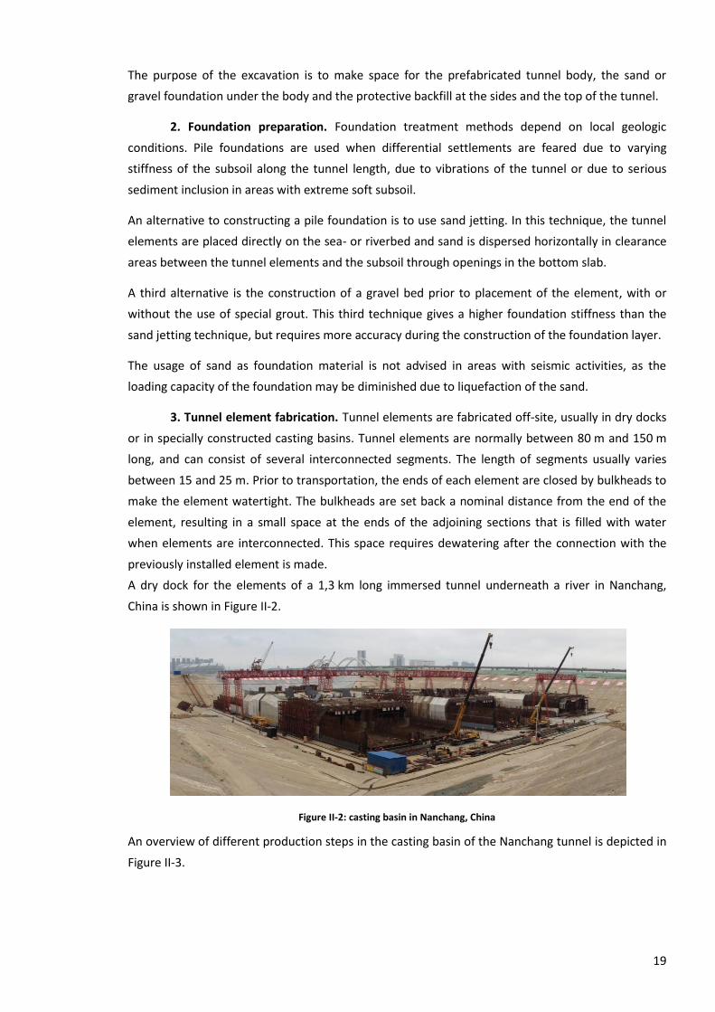
A dry dock for the elements of a 1,3 km long immersed tunnel underneath a river in Nanchang,

China is shown in Figure II-2.

Figure II-2: casting basin in Nanchang, China

An overview of different production steps in the casting basin of the Nanchang tunnel is depicted in

Figure II-3.

20

Figure II-3: production steps in casting basin of Nanchang project (November 2015)

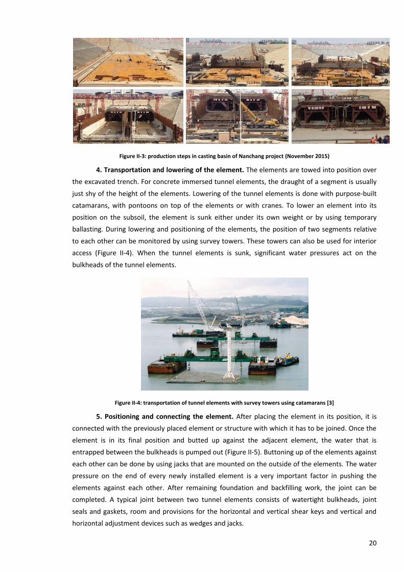
4. Transportation and lowering of the element. The elements are towed into position over

the excavated trench. For concrete immersed tunnel elements, the draught of a segment is usually

just shy of the height of the elements. Lowering of the tunnel elements is done with purpose-built

catamarans, with pontoons on top of the elements or with cranes. To lower an element into its

position on the subsoil, the element is sunk either under its own weight or by using temporary

ballasting. During lowering and positioning of the elements, the position of two segments relative

to each other can be monitored by using survey towers. These towers can also be used for interior

access (Figure II-4). When the tunnel elements is sunk, significant water pressures act on the

bulkheads of the tunnel elements.

Figure II-4: transportation of tunnel elements with survey towers using catamarans [3]

5. Positioning and connecting the element. After placing the element in its position, it is

connected with the previously placed element or structure with which it has to be joined. Once the

element is in its final position and butted up against the adjacent element, the water that is

entrapped between the bulkheads is pumped out (Figure II-5). Buttoning up of the elements against

each other can be done by using jacks that are mounted on the outside of the elements. The water

pressure on the end of every newly installed element is a very important factor in pushing the

elements against each other. After remaining foundation and backfilling work, the joint can be

completed. A typical joint between two tunnel elements consists of watertight bulkheads, joint

seals and gaskets, room and provisions for the horizontal and vertical shear keys and vertical and

horizontal adjustment devices such as wedges and jacks.

21

Figure II-5: positioning adjacent elements and dewatering voids between bulkheads [5]

6. Backfilling the trench. A locking fill (sand or coarser material) is placed in the trench to

about half the height of the elements to ensure their position after connection. Ordinary backfill is

also placed to fill the trench, to a depth of about 1,5 m to maximum 2 m above the tube. This

ordinary backfill is typically material that was excavated from the trench. The ballast on top of the

tunnel functions as a protection of the structure and also prevents uplift.

Figure II-6: backfill material is laced besides and over the tunnel [3]

7. Complementary works in the tunnel. As soon as the tunnel elements have been brought

to rest on the permanent foundation and after the ballast has been applied to prevent uplift, the

complementary works inside the tunnel can be performed. They include casting of ballast concrete

and removal of water in the tunnel, installation of remaining seals and joints and construction of

the remaining joint structure. The installation of shear keys in the element joints is done in this

phase of the tunnel construction.

4.2 Immersed joints

An immersed joint consists of structural mechanisms to transfer loads across the joint, and

elements to ensure watertightness of the joint.

4.2.1 Structural configuration

The transfer of non-axial loads over the segment joint is ensured by horizontal and vertical shear

keys (either in concrete or in steel). Longitudinal compression forces are transferred through infill

concrete between the adjacent elements and through the Gina gasket. In case they occur, extension

forces in the longitudinal direction of the tunnel can be transferred with passive or pre-stressed

cables.

To clarify the structural configuration of immersion joints, some practical examples from existing

projects are mentioned.

22

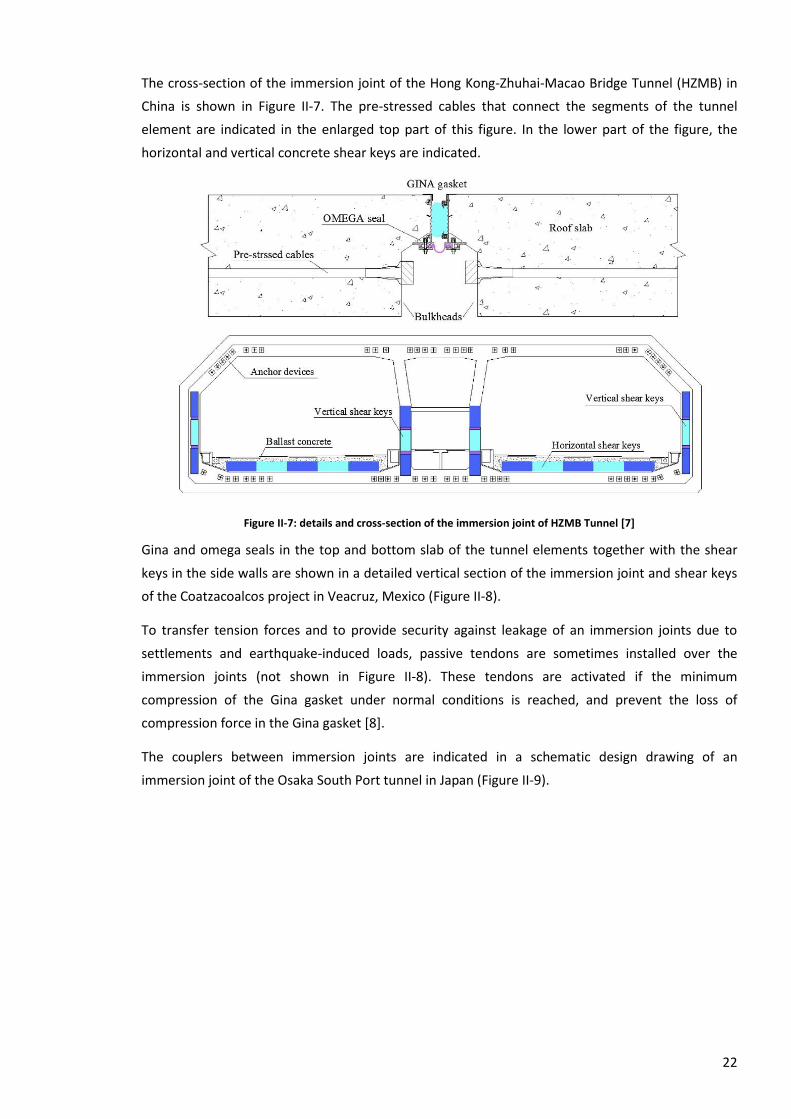
The cross-section of the immersion joint of the Hong Kong-Zhuhai-Macao Bridge Tunnel (HZMB) in

China is shown in Figure II-7. The pre-stressed cables that connect the segments of the tunnel

element are indicated in the enlarged top part of this figure. In the lower part of the figure, the

horizontal and vertical concrete shear keys are indicated.

Figure II-7: details and cross-section of the immersion joint of HZMB Tunnel [7]

Gina and omega seals in the top and bottom slab of the tunnel elements together with the shear

keys in the side walls are shown in a detailed vertical section of the immersion joint and shear keys

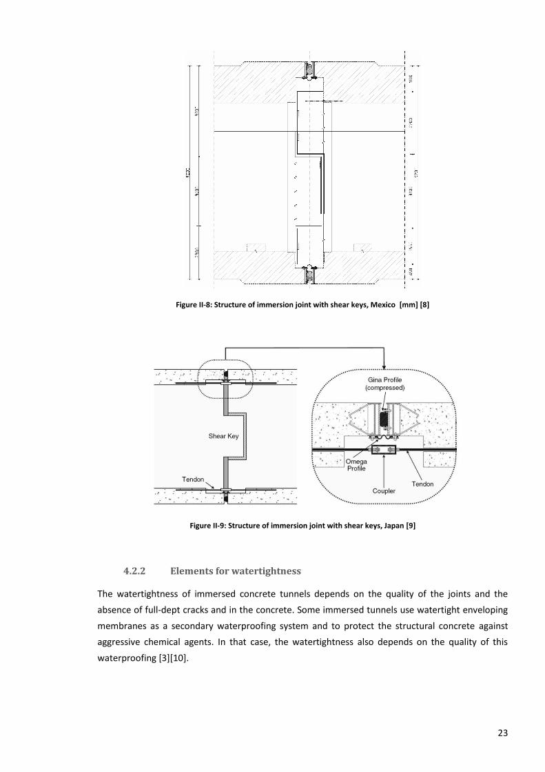
of the Coatzacoalcos project in Veacruz, Mexico (Figure II-8).

To transfer tension forces and to provide security against leakage of an immersion joints due to

settlements and earthquake-induced loads, passive tendons are sometimes installed over the

immersion joints (not shown in Figure II-8). These tendons are activated if the minimum

compression of the Gina gasket under normal conditions is reached, and prevent the loss of

compression force in the Gina gasket [8].

The couplers between immersion joints are indicated in a schematic design drawing of an

immersion joint of the Osaka South Port tunnel in Japan (Figure II-9).

23

Figure II-8: Structure of immersion joint with shear keys, Mexico [mm] [8]

Figure II-9: Structure of immersion joint with shear keys, Japan [9]

4.2.2 Elements for watertightness

The watertightness of immersed concrete tunnels depends on the quality of the joints and the

absence of full-dept cracks and in the concrete. Some immersed tunnels use watertight enveloping

membranes as a secondary waterproofing system and to protect the structural concrete against

aggressive chemical agents. In that case, the watertightness also depends on the quality of this

waterproofing [3][10].

24

To ensure this watertightness of joints, water seals and gaskets are installed in the immersed joints.

All joints between the tunnel elements are to be tightly closed. The use of rubber seals makes it

possible to maintain some degree of flexibility of the immersed joints.

Waterstop gaskets are installed prior to floating of the tunnel elements and they provide an initial

seal upon connection of the elements after sinking. For this primary watertight sealing, different

types are used worldwide. In the 1960's, the Gina sealing was invented in the Netherlands [11].

Different types of gaskets are shown in Figure II-10. In this figure, (a) and (c) are Gina gaskets, which

are common in Western Europe and in China.

Figure II-10: different kind of waterstop gaskets [11]

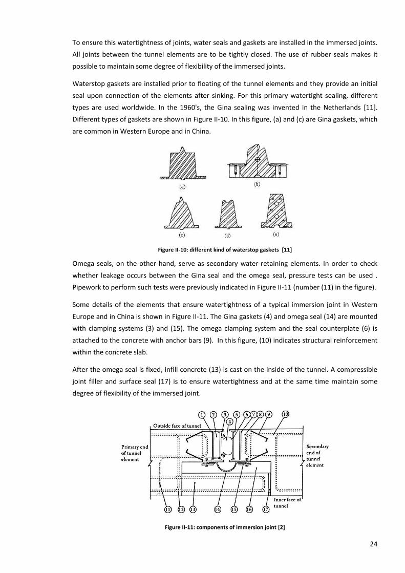
Omega seals, on the other hand, serve as secondary water-retaining elements. In order to check

whether leakage occurs between the Gina seal and the omega seal, pressure tests can be used .

Pipework to perform such tests were previously indicated in Figure II-11 (number (11) in the figure).

Some details of the elements that ensure watertightness of a typical immersion joint in Western

Europe and in China is shown in Figure II-11. The Gina gaskets (4) and omega seal (14) are mounted

with clamping systems (3) and (15). The omega clamping system and the seal counterplate (6) is

attached to the concrete with anchor bars (9). In this figure, (10) indicates structural reinforcement

within the concrete slab.

After the omega seal is fixed, infill concrete (13) is cast on the inside of the tunnel. A compressible

joint filler and surface seal (17) is to ensure watertightness and at the same time maintain some

degree of flexibility of the immersed joint.

Figure II-11: components of immersion joint [2]

25

Part of the clamping system for the Gina gaskets on an element under construction of the Nanchang

project is indicated with arrows in Figure II-12.

Figure II-12: Mounting system for Gina seal in Nanchang project

In order to avoid full-depth cracks in the structural concrete (due to, for example, shrinkage), the

tunnel elements can be composed of different segments, that are interconnected with expansion

joints. The length of each segment depends on the practical length of a single concrete pour and of

the risk for shrinkage cracks, and is typically in the range of 20 m. The vertical joint between two

segments is provided with a cast-in flexible waterstop (Figure II-13). In this way, the tunnel element

can be subjected to flexural deformations without developing longitudinal tensile strain at the

location of the expansion joints, which may cause cracking of the concrete. Longitudinal pre-

stressing is also sometimes applied to avoid uncontrollable full-depth cracks. Crack inducers at the

location of the segment joints can force tensile cracks to occur at the location of segment joints. For

the Coatzacoalcos project, an injection hole at the location of the segment joints allow for the

repair of such cracks [7][8][10].

Figure II-13: example of an expansion joint between 2 segments [mm] [10]

An example of rubber waterstops that ensure watertightness between two different casts in the

Nanchang project is shown in the middle of Figure II-14.

26

Figure II-14: Rubber waterstops used to ensure watertightness between two casts in the Nanchang project

4.2.3 Shear keys

Shear keys of immersed tunnel have a dual purpose: to avoid discontinuous displacements over the

immersed joints in longitudinal and vertical direction, and to transfer shear forces between the

tunnel elements. Since neither the water seals, nor longitudinal tendons over immersion joints are

suited to take up shear, the transfer of shear forces is the primary function of the shear keys.

The structural configuration of the immersion joint of the HZMB Tunnel in China and a

representation of the shear keys in the walls of the Coatzacoalcos project in Veacruz, Mexico were

shown in Figure II-7 and Figure II-8.

The vertical shear keys transfer shear forces between adjacent joint under longitudinal bending,

and the horizontal concrete reinforced shear keys in the ballasted concrete bear horizontal forces,

such as seismic shear forces. The pre-stressed cables will work in for example during seismic events

and keep the displacements of segmental joints within their waterproofing limits. Shear key forces

can also be expected as a result of foundation stiffness variations, sedimentation loads on the

tunnel or gravel bed surface intolerances [7][12].

During transportation and positioning of elements, segments are held together by using

longitudinal tendons in order to maintain the integrity of the tunnel element. The tendons can be

either passive or pre-stressed. If the tendons are pre-stressed, the differential displacements at the

immersion joints can be expected to be lower than in the case where the tendons are passive. The

latter case requires more heavy shear keys [8].

The dimensions of the shear keys are an important design issue for the overall tunnel structure,

because they can be governing for the wall thickness and the overall structural dimensions of the

tunnel [12].

For the Nanchang project, provisions to attach the vertical steel shear keys prior to sinking are

shown in Figure II-15.

27

Figure II-15: provisions to attach vertical shear keys in Nanchang project

The horizontal concrete shear keys are only installed after sinking and connecting of the elements.

Again for the Nanchang project, a schematic view of the vertical steel rebars with which the

concrete shear keys are connected to the ends of the tunnel elements is shown in Figure II-16.

Figure II-16: concrete shear key connection rebars in the Nanchang Red Valley immersed joint (side view) [mm]

28

III Design starting points

In this chapter the design starting points for the physical scale model and so also for the FE model

are elaborated.

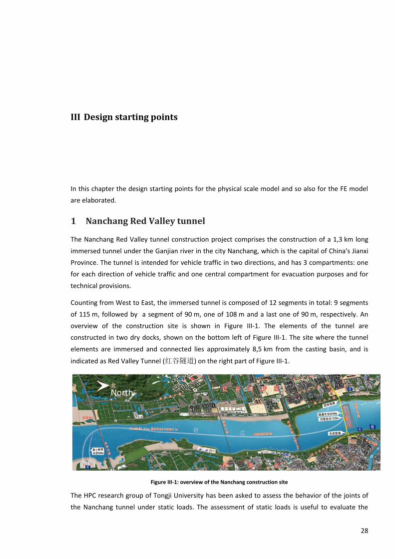
1 Nanchang Red Valley tunnel

The Nanchang Red Valley tunnel construction project comprises the construction of a 1,3 km long

immersed tunnel under the Ganjian river in the city Nanchang, which is the capital of China's Jianxi

Province. The tunnel is intended for vehicle traffic in two directions, and has 3 compartments: one

for each direction of vehicle traffic and one central compartment for evacuation purposes and for

technical provisions.

Counting from West to East, the immersed tunnel is composed of 12 segments in total: 9 segments

of 115 m, followed by a segment of 90 m, one of 108 m and a last one of 90 m, respectively. An

overview of the construction site is shown in Figure III-1. The elements of the tunnel are

constructed in two dry docks, shown on the bottom left of Figure III-1. The site where the tunnel

elements are immersed and connected lies approximately 8,5 km from the casting basin, and is

indicated as Red Valley Tunnel (红谷隧道) on the right part of Figure III-1.

Figure III-1: overview of the Nanchang construction site

The HPC research group of Tongji University has been asked to assess the behavior of the joints of

the Nanchang tunnel under static loads. The assessment of static loads is useful to evaluate the

29

structural behavior of the immersed joint, for example to find the internal force distribution of

loads over the internal load-carrying parts of the immersed joint. Also, during seismic analyses

seismic loads are commonly translated in to static loads. A first step in the assessment of the

Nanchang tunnel segments under seismic loading thus can thus be to investigate the behavior of

the segments under static loading.

In order to assess the behavior of the Nanchang Red Valley immersed tunnel under static loads, two

modeling techniques are used: performing numerical analyses on a geometrically scaled Abaqus FE

software model and by performing a 1:5 physical scale model test at the Nanchang construction

site. The aim of the numerical model is to predict the behavior of the physical scale model.

2 Immersed joint shear key configuration

Both the physical scale model and the numerical model of the Nanchang Red Valley immersed

tunnel are based on the final design plans for the actual construction project of the tunnel

prototype. Some parts of the design of the actual construction project on which both models are

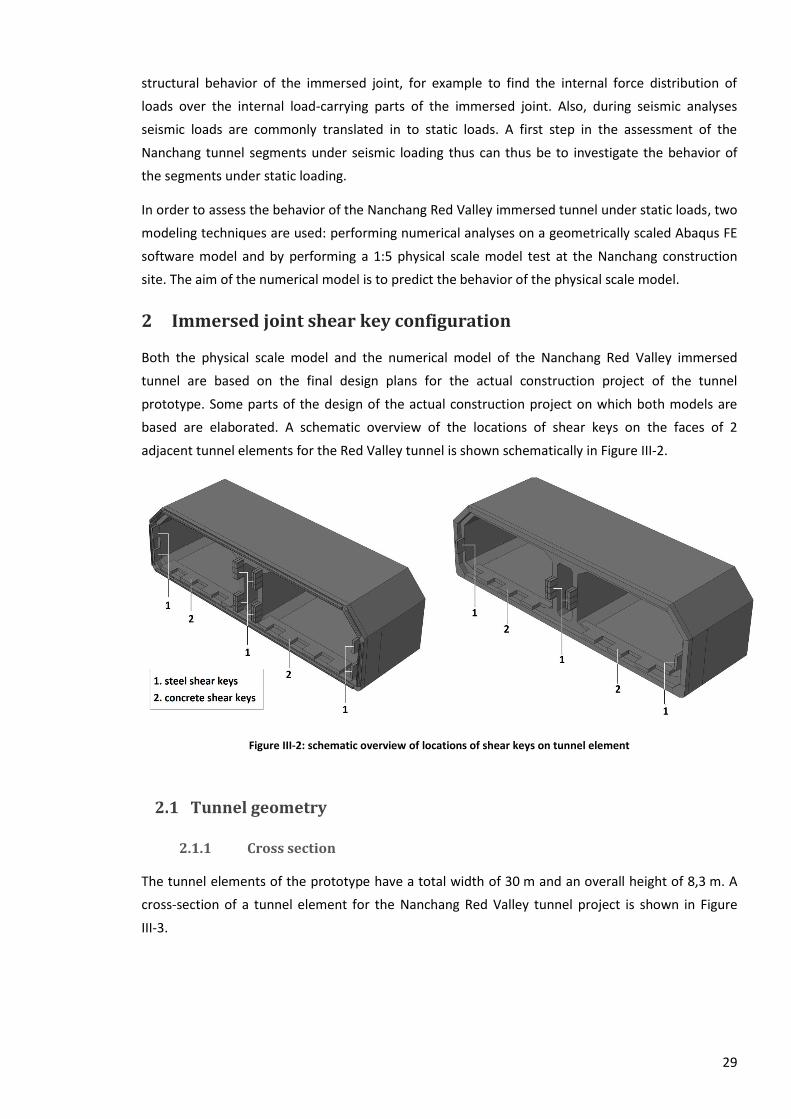
based are elaborated. A schematic overview of the locations of shear keys on the faces of 2

adjacent tunnel elements for the Red Valley tunnel is shown schematically in Figure III-2.

Figure III-2: schematic overview of locations of shear keys on tunnel element

2.1 Tunnel geometry

2.1.1 Cross section

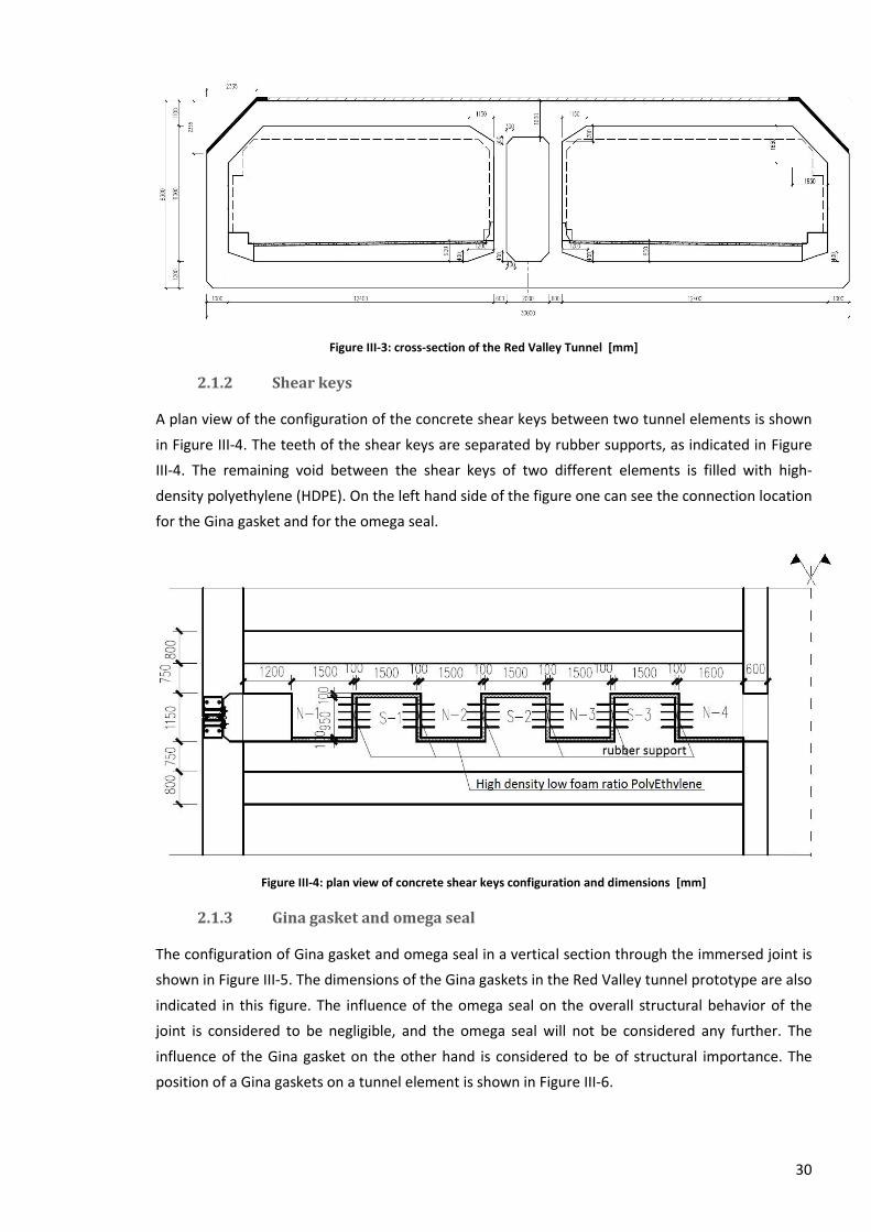
The tunnel elements of the prototype have a total width of 30 m and an overall height of 8,3 m. A

cross-section of a tunnel element for the Nanchang Red Valley tunnel project is shown in Figure

III-3.

30

Figure III-3: cross-section of the Red Valley Tunnel [mm]

2.1.2 Shear keys

A plan view of the configuration of the concrete shear keys between two tunnel elements is shown

in Figure III-4. The teeth of the shear keys are separated by rubber supports, as indicated in Figure

III-4. The remaining void between the shear keys of two different elements is filled with high-

density polyethylene (HDPE). On the left hand side of the figure one can see the connection location

for the Gina gasket and for the omega seal.

Figure III-4: plan view of concrete shear keys configuration and dimensions [mm]

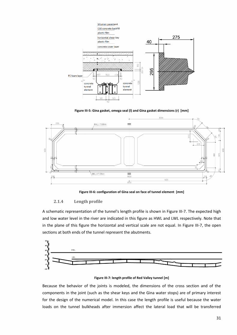
2.1.3 Gina gasket and omega seal

The configuration of Gina gasket and omega seal in a vertical section through the immersed joint is

shown in Figure III-5. The dimensions of the Gina gaskets in the Red Valley tunnel prototype are also

indicated in this figure. The influence of the omega seal on the overall structural behavior of the

joint is considered to be negligible, and the omega seal will not be considered any further. The

influence of the Gina gasket on the other hand is considered to be of structural importance. The

position of a Gina gaskets on a tunnel element is shown in Figure III-6.

31

Figure III-5: Gina gasket, omega seal (l) and Gina gasket dimensions (r) [mm]

Figure III-6: configuration of Gina seal on face of tunnel element [mm]

2.1.4 Length profile

A schematic representation of the tunnel's length profile is shown in Figure III-7. The expected high

and low water level in the river are indicated in this figure as HWL and LWL respectively. Note that

in the plane of this figure the horizontal and vertical scale are not equal. In Figure III-7, the open

sections at both ends of the tunnel represent the abutments.

Figure III-7: length profile of Red Valley tunnel [m]

Because the behavior of the joints is modeled, the dimensions of the cross section and of the

components in the joint (such as the shear keys and the Gina water stops) are of primary interest

for the design of the numerical model. In this case the length profile is useful because the water

loads on the tunnel bulkheads after immersion affect the lateral load that will be transferred

32

though the immersed joint. An assessment of these loads for the tunnel prototype has been made

in the design stage of the tunnel prototype, and is discussed below.

2.2 Axial load

Under the influence of lateral loads on the side of a tunnel element, the concrete shear keys will be

loaded most heavily when the axial load on the tunnel face is minimal. When this is the case, the

forces that the Gina gaskets exert on the opposite tunnel element is also minimal. According to

Coulomb's friction law, this reduces the friction between the Gina gasket and the tunnel face. This

has as a result that more load is taken up by the concrete shear keys. One of the loads that is of

importance to model the behavior of the concrete shear keys is thus the minimal vertical load on

the bulkheads.

A preliminary assessment of the total axial water load on the bulkheads of the Red Valley tunnel

just after sinking was made by the Dutch firm Trelleborg. Their results are attached in Addendum I.

These results, that are based on historic data of water heights in the Ganjian river, show that the

lowest load that is to be expected on a bulkhead just after sinking is 8779 kN. This value will be

used to determine the loads that are used in the numerical and physical modeling.

33

IV Numerical modeling of the Red Valley tunnel

Numerical modeling of the Red Valley tunnel is conducted using FE software package Abaqus. Just

like the physical scale model, the dimensions of the numerical model are downscaled geometrically

by a factor 5 compared to the actual Red Valley tunnel construction project (prototype). This way,

the dimensions in the numerical model and the dimensions of the scale model are the same, and

results of the numerical simulation can be compared directly to the results of the scale model

without taking into account further scaling effects between both models.

Only the behavior of the immersed joint is simulated, so both the numerical model and the physical

scale model comprise 2 adjacent tunnel elements and their common connection. The joint of the

numerical model contains Gina gaskets, concrete shear keys with rebars but contrary to the physical

model, the numerical model does not contain steel shear keys (cf. infra).

1 The Abaqus software package

Abaqus is a suite of engineering simulation programs based on the FE method. With Abaqus both

linear and nonlinear simulations of structural systems can be performed, with a wide range of

materials. In a nonlinear analysis Abaqus automatically chooses appropriate load increments to

ensure that an accurate solution is obtained. For the simulation of concrete shear key behavior, the

package Abaqus/Standard is used. This is a general-purpose analysis suited for solving static

responses. Contrary to Abaqus/Explicit, the Abaqus/Standard package solves a system of equations

implicitly at each load increment, performing iterations until the solution converges. It has a wide

range of material models and has a robust capacity for solving contact problems, and its solution

technique is unconditionally stable [13].

The model is preprocessed with the product Abaqus/CAE. This is an interactive graphical

environment in which geometries are created and/or imported, and meshed. The material

properties, interaction properties, loads and boundary conditions are assigned to the geometry in

Abaqus/CAE. It is also used to submit the analysis and to do the postprocessing.

34

2 Model design

2.1 Dimensional similitude

The scale factor for geometric length of both the physical and numerical model is 1:5. This implies a

scale factor of 1/5 for all length quantities, or SL = 1/5. The scale factor for displacements is chosen

to be equal to the scale factor for length (Sx = SL). The scale model will use the same materials as the

actual prototype, which implies that the E-moduli of the materials in the models and prototype will

be identical. This implies SE = 1. From the 3 similitude parameters SL, Sx and SE, all other necessary

similitude parameters can be obtained. The similitude parameters for the FE model (and also for the

physical scale model) are shown in Table IV-1.

Table IV-1: model similitude analysis for numerical model and scale model

quantity dimensions scale factor

geometry

length L SL 1/5

displacement x Sx = SL 1/5

area - SL² 1/25

volume L³ SL³ 1/125

material

stress FL-2 SE 1

strain - - 1

E-modulus FL-2 SE 1

Poisson ratio - - 1

load

point load F SE SL² 1/25

distributed load FL-1 SE SL 1/5

area load FL-2 SE 1

moment FL SE SL³ 1/125

2.2 Model geometry

The cross-section of the numerical model is scaled geometrically by a factor SL = 1/5 compared to

the Nanchang Red Valley tunnel prototype. All dimensions that were mentioned in part III are

downscaled by a factor 5, and no changes are made to the overall geometry of the tunnel cross

section. An overview of the 2 segments out of which the numerical model is composed was shown

previously in Figure III-2 (page 29), with the difference that the steel shear keys are omitted in the

numerical model. The rubber supports between the concrete shear keys are also not included in the

numerical model. The dimensions of the cross sections of the two tunnel elements are depicted in

Figure IV-1. In this figure, the positioning of the concrete shear keys relative to the cross section of

the tunnel elements is also indicated for the numerical model. The tunnel elements of both the

numerical model and scale model have a depth of 1800 mm measured perpendicular to the plane

of Figure IV-1. The dimensions of the concrete shear keys of the FE model are depicted in Figure

IV-2. A plan view of the configuration of the concrete shear keys and their dimensions in the

numerical model is shown in Figure IV-3. A drawing of the reinforcement bars in the numerical

model's concrete shear keys is shown in Figure IV-4. The configuration of the reinforcement bars in

35

the shear keys in the FE model is taken the same as the configuration in the design of the physical

scale model test.

Figure IV-1: cross-section for physical scale model and numerical model [mm]

Figure IV-2: plan view and front view of concrete shear keys configuration and dimensions for numerical model [mm]

Figure IV-3: positioning of concrete shear keys in plan view [mm]

36

Figure IV-4: numerical model concrete shear key reinforcement [mm]

2.3 Boundary conditions

The boundary conditions of the overall numerical model are depicted in Figure IV-5. A convention

for the numbering of the two tunnel elements (1 and 2) is also shown in this figure. The bottom part

of tunnel element 1 is constrained so it cannot move in the vertical (y-) direction. Rigid body

translation of tunnel element 2 is prevented by constraining the indicated area of tunnel element 2

in all three the x-, y- and z-directions (Figure IV-5). These boundary conditions are defined to mimic

the boundary conditions of the physical scale model on the Nanchang construction site and do not

take into account certain phenomena that might occur with the tunnel prototype. For example

differential settlements just after immersion of the tunnel elements is not considered, and thus

spring boundary conditions are not considered.

Figure IV-5: numerical model boundary conditions

To model the connection between the concrete shear keys and the tunnel elements, tie constraints

are used. This means that the relative displacement of all points that the common points on the

surfaces of the concrete shear keys and the tunnel elements is set to be zero in all directions. The

37

same technique is used to model the connection between the Gina gaskets and the concrete tunnel

elements.

In the numerical simulation the Gina seal is modeled using six separate straight Gina gaskets. In the

tunnel prototype as well as in the physical scale model, the Gina seal is composed of one large part

that is connected in a continuous manner to tunnel element 2 (see also Figure III-6 on p. 31). In

order to model interaction between the separate parts out of which the Gina seal is composed, the

faces that make up the boundaries between the different Gina parts are assigned local boundary

conditions stating that these faces can have no movement out of their plane. Referring to Figure

IV-6 this means that the hatched surface on the horizontal shear key cannot move in the

x-direction, the hatched surface on the vertical shear key cannot move in the y-direction and the

hatched areas on the tilted Gina cannot move in the local z'-direction. This simplification of the

connections may introduce a more stiff behavior of the Gina seals in the x-y-plane of the numerical

model. The effect hereof to the overall solution is assumed to be negligible.

Figure IV-6: Gina gasket local boundary conditions

2.4 Loads

2.4.1 Considered loading case

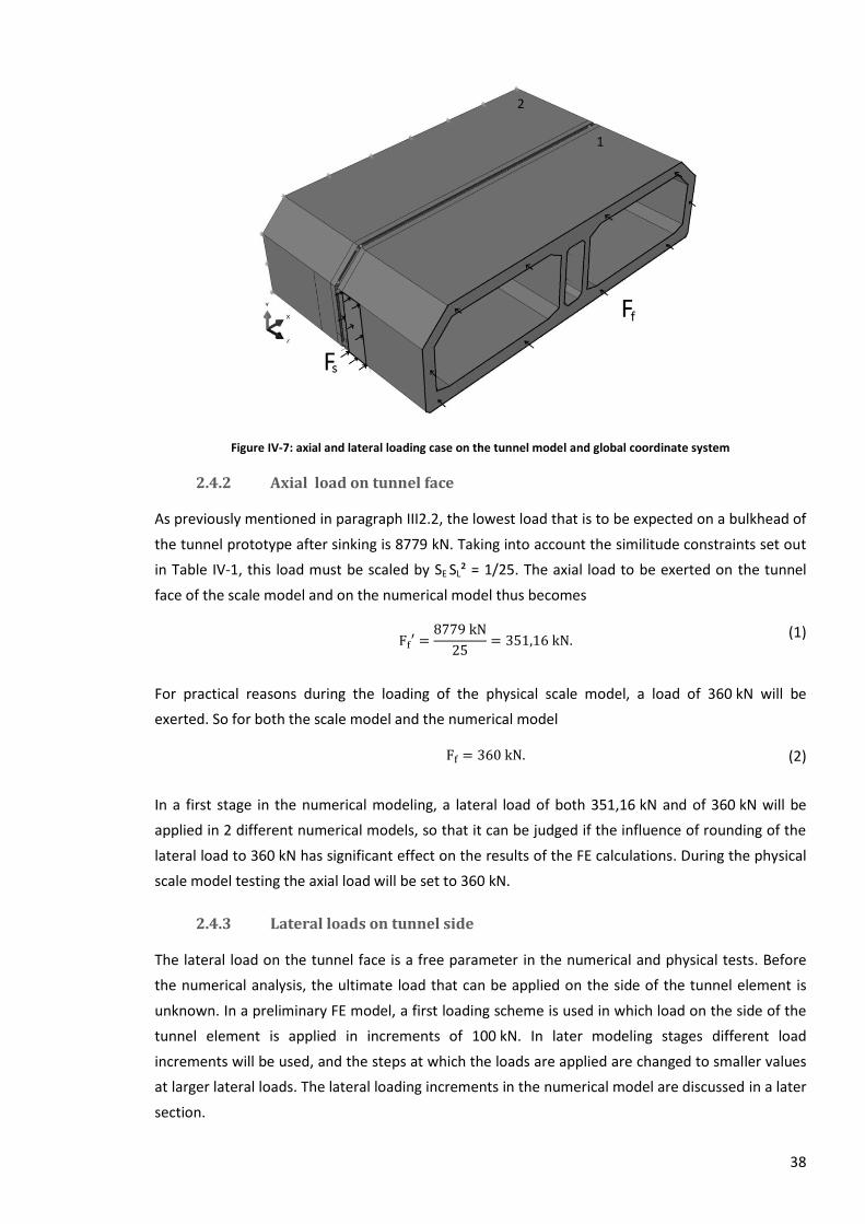
The load case under investigation in both the numerical and physical scale model is depicted in

Figure IV-7. The global coordinate system that will be used throughout the analysis is depicted on

the left hand side in Figure IV-7. The x-direction is defined as the lateral direction and the z-

direction as the longitudinal one. The y-direction is defined as the vertical direction. The loading

case consists of an axial load Ff on the tunnel face of tunnel element 1 and a lateral load Fs on the

tunnel side of element 1. During the analysis, Ff is held constant and Fs is increased incrementally up

to the point where complete damage of the concrete shear keys occurs. In the physical scale model

test, the horizontal load on the side of the tunnel will be applied through a steal beam with a flange

with of 400 mm. Therefore the load on the side of tunnel element Fs in the numerical model is also

applied over a rectangular area with a width of 400 mm along the z-axis.

38

Figure IV-7: axial and lateral loading case on the tunnel model and global coordinate system

2.4.2 Axial load on tunnel face

As previously mentioned in paragraph III2.2, the lowest load that is to be expected on a bulkhead of

the tunnel prototype after sinking is 8779 kN. Taking into account the similitude constraints set out

in Table IV-1, this load must be scaled by SE SL² = 1/25. The axial load to be exerted on the tunnel

face of the scale model and on the numerical model thus becomes

(1)

For practical reasons during the loading of the physical scale model, a load of 360 kN will be

exerted. So for both the scale model and the numerical model

(2)

In a first stage in the numerical modeling, a lateral load of both 351,16 kN and of 360 kN will be

applied in 2 different numerical models, so that it can be judged if the influence of rounding of the

lateral load to 360 kN has significant effect on the results of the FE calculations. During the physical

scale model testing the axial load will be set to 360 kN.

2.4.3 Lateral loads on tunnel side

The lateral load on the tunnel face is a free parameter in the numerical and physical tests. Before

the numerical analysis, the ultimate load that can be applied on the side of the tunnel element is

unknown. In a preliminary FE model, a first loading scheme is used in which load on the side of the

tunnel element is applied in increments of 100 kN. In later modeling stages different load

increments will be used, and the steps at which the loads are applied are changed to smaller values

at larger lateral loads. The lateral loading increments in the numerical model are discussed in a later

section.

39

3 Materials and interaction behavior

To ease the construction process of the scale model on the construction site, the concrete and steel

types used in the physical scale model will be the same as concrete and steel types used in the

construction of the actual Red Valley tunnel construction.

The concrete type for both the tunnel elements and the concrete shear keys used in the physical

scale model is C40. The properties of this material are shown in Table IV-2. The concrete in the

FE model is modeled using these parameters. Other concrete parameters are explained in

paragraph IV3.1.

The steel type used for the rebars in the concrete shear keys is Q345. The elastic parameters that

are used for the steel rebars in the numerical model are shown in Table IV-3.

The description of the rubber material is discussed further on in paragraph IV3.4.

Table IV-2: plain concrete material parameters

concrete type C40 mass density 2,40E-06 [kg/mm³]

Young's modulus 32500 [N/mm²]

Poisson ratio 0,2 [-]

Table IV-3: steel reinforcement material parameters

steel type Q345 mass density 7,84E-06 [kg/mm³]

Young's modulus 203000 [N/mm²]

Poisson ratio 0,3 [-]

For all materials in the FE model C3D8R elements are used, except for the steel rebars, who are

composed of beam elements. The C3D8R element in Abaqus is an 8-node linear brick element with

reduced integration, and is used with hourglass control to avoid zero-energy modes. For the steel

rebars the T3D2 element type is used. These are linear 3D-truss elements with nodes at each end of

each reinforcement bar.

3.1 Plain concrete material model

There are three material models that are commonly used to simulate the behavior of plain and

reinforced concrete in Abaqus: the concrete cracking model, the concrete smeared cracking model

and the concrete damaged plasticity model [13]. For the numerical model of the Nanchang Red

Valley tunnel, a concrete damaged plasticity model is used. This model is chosen because, unlike the

concrete smeared cracking model, it can be used without having to assume monotonic straining of

the concrete element under examination. Furthermore the concrete damaged plasticity model

allows for nonlinear behavior both in tension and in compression. Contrary to the cracking model

for concrete, it takes into account both tensile cracking and compressive failure.

The concrete damaged plasticity model assumes low confining pressures, which is assumed to be

the case in the loading scheme of the Red Valley model tests. In order to explain certain parameters

40

that occur in the material model, a brief overview of the governing constitutive relations is

provided, based entirely on the plastic damage model for concrete by Lubliner (1988) and by Lee

and Fenves (1998) [14][15][16][17]. The uniaxial loading case is formulated first, and is then

extended to the multiaxial case. In the preprocessing stage of the numerical model, the uniaxial

case is most important because the damaged plasticity model in Abaqus requires uniaxial

parameters as input. Abaqus automatically converts these parameters to the multiaxial case, that is

also explained briefly.

3.1.1 Uniaxial loading

The concrete damaged plasticity model assumes a decomposition of the strain into an elastic part

and a plastic part :

(3)

The assumed behavior of concrete in uniaxial tension and compression is shown in Figure IV-8 and

Figure IV-9. The material behavior is such that for both the compression and the tension case, the

initial elastic stiffness E0 is reduced when the softening branch is reached. This reduction of the

initial stiffness is proportional to the damage that occurs in the concrete material and is reflected

into the constitutive relations by the damage parameters dt and dc, where subscripts t and c denote

tension and compression, respectively. Both damage parameters are scalar degradation variables

that range from 0 to 1, where the value 0 denotes no damage and the value 1 denotes fully

damaged material.

For the uniaxial case,

and

are the equivalent plastic strains in tension and compression, and

characterize the damaged state of the material. and

are defined as the cracking strain in

tension and the inelastic (crushing) strain in compression, respectively.

The stress-strain relations under uniaxial tension and compression loading are (Figure IV-8 and

Figure IV-9):

(4)

(5)

The yield condition in the multiaxial case will in a later paragraph be defined in terms of effective

uniaxial stresses, which are defined as

(6)

(7)

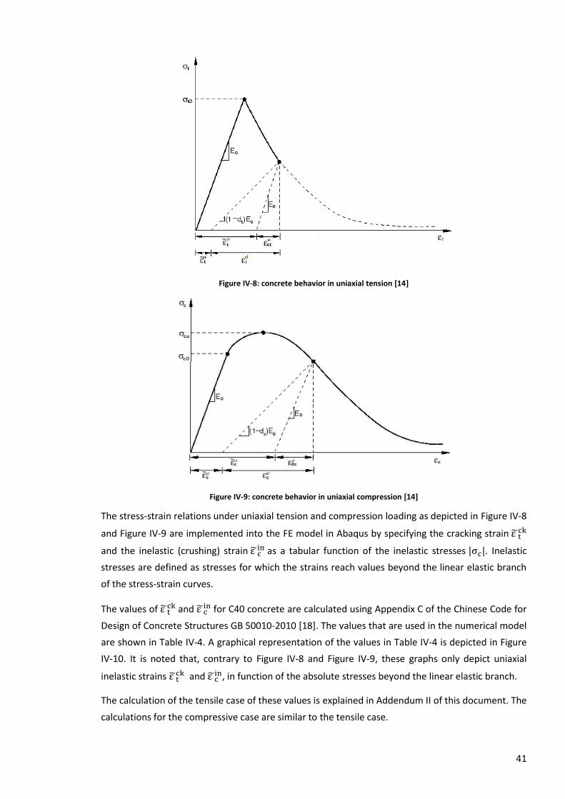
41

Figure IV-8: concrete behavior in uniaxial tension [14]

Figure IV-9: concrete behavior in uniaxial compression [14]

The stress-strain relations under uniaxial tension and compression loading as depicted in Figure IV-8

and Figure IV-9 are implemented into the FE model in Abaqus by specifying the cracking strain

and the inelastic (crushing) strain as a tabular function of the inelastic stresses . Inelastic

stresses are defined as stresses for which the strains reach values beyond the linear elastic branch

of the stress-strain curves.

The values of and

for C40 concrete are calculated using Appendix C of the Chinese Code for

Design of Concrete Structures GB 50010-2010 [18]. The values that are used in the numerical model

are shown in Table IV-4. A graphical representation of the values in Table IV-4 is depicted in Figure

IV-10. It is noted that, contrary to Figure IV-8 and Figure IV-9, these graphs only depict uniaxial

inelastic strains and

, in function of the absolute stresses beyond the linear elastic branch.

The calculation of the tensile case of these values is explained in Addendum II of this document. The

calculations for the compressive case are similar to the tensile case.

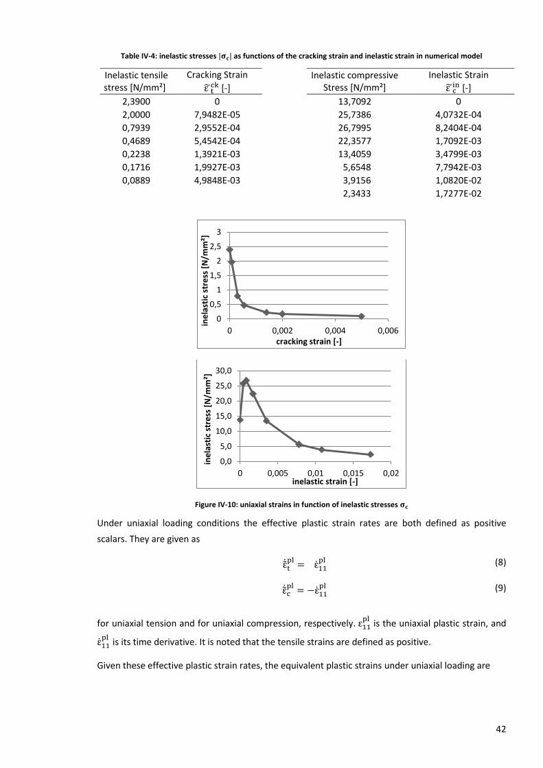
42

Table IV-4: inelastic stresses as functions of the cracking strain and inelastic strain in numerical model

Inelastic tensile stress [N/mm²]

Cracking Strain

[-]

Inelastic compressive Stress [N/mm²]

Inelastic Strain

[-]

2,3900 0

13,7092 0

2,0000 7,9482E-05

25,7386 4,0732E-04

0,7939 2,9552E-04

26,7995 8,2404E-04

0,4689 5,4542E-04

22,3577 1,7092E-03

0,2238 1,3921E-03

13,4059 3,4799E-03

0,1716 1,9927E-03

5,6548 7,7942E-03

0,0889 4,9848E-03

3,9156 1,0820E-02

2,3433 1,7277E-02

Figure IV-10: uniaxial strains in function of inelastic stresses

Under uniaxial loading conditions the effective plastic strain rates are both defined as positive

scalars. They are given as

(8)

(9)

for uniaxial tension and for uniaxial compression, respectively.

is the uniaxial plastic strain, and

is its time derivative. It is noted that the tensile strains are defined as positive.

Given these effective plastic strain rates, the equivalent plastic strains under uniaxial loading are

0

0,5

1

1,5

2

2,5

3

0 0,002 0,004 0,006

ine

last

ic s

tre

ss [

N/m

m²]

cracking strain [-]

0,0

5,0

10,0

15,0

20,0

25,0

30,0

0 0,005 0,01 0,015 0,02

ine

last

ic s

tre

ss [

N/m

m²]

inelastic strain [-]

43

(10)

(11)

where the integration is carried out over the time step over which the numerical calculation is

performed. For the analysis at hand, typical time steps are between 10-4 sec and 0,25 sec.

Equations (8)-(11) define the equivalent plastic strains under uniaxial loading conditions. As shown

in Figure IV-8 and Figure IV-9, the degradation of the elastic stiffness is characterized by the two

uniaxial damage variables and , who are assumed to be mutually independent. These damage

variables are assumed to be a direct function of the equivalent plastic strains:

(12)

(13)

For the practical implementation of the concrete damaged plasticity model in Abaqus, the damage

variables and are defined directly as tabular functions of the cracking strain and inelastic

crushing strain and

. The tabular functions that are implemented in the numerical model are

mentioned in Table IV-5. These values are for concrete C40 and were calculated on the basis of

Appendix C of the Chinese code for design of concrete structures GB 50010-2010 [18] (see also

Addendum II). The numerical values in Table IV-5 are depicted graphically in Figure IV-11.

Because the constitutive relations for tensile behavior are based on damage parameters in function

of the equivalent plastic strain, Abaqus has to convert the cracking strain values to equivalent

plastic strains. Based on Figure IV-8, the relation between the cracking strain values and the

plastic strain values

is

(14)

Similarly for the compressive case the relation between the inelastic strain values and the

inelastic (crushing) strain is

(15)

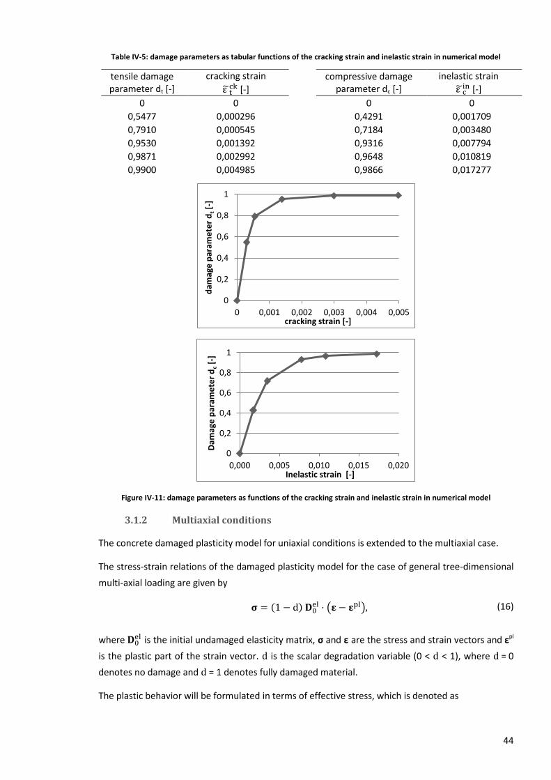
44

Table IV-5: damage parameters as tabular functions of the cracking strain and inelastic strain in numerical model

tensile damage parameter dt [-]

cracking strain

[-]

compressive damage parameter dc [-]

inelastic strain

[-]

0 0

0 0

0,5477 0,000296

0,4291 0,001709

0,7910 0,000545

0,7184 0,003480

0,9530 0,001392

0,9316 0,007794

0,9871 0,002992

0,9648 0,010819

0,9900 0,004985

0,9866 0,017277

Figure IV-11: damage parameters as functions of the cracking strain and inelastic strain in numerical model

3.1.2 Multiaxial conditions

The concrete damaged plasticity model for uniaxial conditions is extended to the multiaxial case.

The stress-strain relations of the damaged plasticity model for the case of general tree-dimensional

multi-axial loading are given by

(16)

where is the initial undamaged elasticity matrix, σ and ε are the stress and strain vectors and εpl

is the plastic part of the strain vector. d is the scalar degradation variable (0 < d < 1), where d = 0

denotes no damage and d = 1 denotes fully damaged material.

The plastic behavior will be formulated in terms of effective stress, which is denoted as

0

0,2

0,4

0,6

0,8

1

0 0,001 0,002 0,003 0,004 0,005

dam

age

par

ame

ter

dt [

-]

cracking strain [-]

0

0,2

0,4

0,6

0,8

1

0,000 0,005 0,010 0,015 0,020

Dam

age

par

ame

ter

dc

[-]

Inelastic strain [-]

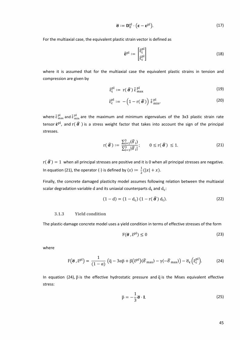
45

(17)

For the multiaxial case, the equivalent plastic strain vector is defined as

(18)

where it is assumed that for the multiaxial case the equivalent plastic strains in tension and

compression are given by

(19)

(20)

where

and

are the maximum and minimum eigenvalues of the 3x3 plastic strain rate

tensor , and is a stress weight factor that takes into account the sign of the principal

stresses.

(21)

when all principal stresses are positive and it is 0 when all principal stresses are negative.

In equation (21), the operator is defined by

.

Finally, the concrete damaged plasticity model assumes following relation between the multiaxial

scalar degradation variable d and its uniaxial counterparts and :

(22)

3.1.3 Yield condition

The plastic-damage concrete model uses a yield condition in terms of effective stresses of the form

(23)

where

(24)

In equation (24), is the effective hydrostatic pressure and is the Mises equivalent effective

stress:

(25)

46

(26)

where

is the deviatory part of the effective stress tensor . is the maximum eigenvalue of . The

function is given by

in which the effective tensile and compressive stresses and

are defined by

equations (6) and (7).

The coefficient α is a dimensionless material constant, and is determined by the initial equibiaxial

compressive yield stress and the initial uniaxial compressive yield stress , as

(27)

The ratio

is an important parameter in the concrete damaged plasticity model in Abaqus.

Typical experimental values of the ratio

range from 1,10 to 1,16 [13][15]. In the numerical

model of the Nanchang Red valley tunnel, a value

= 1,16 is used. This value is based on

investigations by Liu, Xu and Chen [16].

The dimensionless material constant is expressed in the material model in terms of a parameter

:

(28)

where it is reasonable to assume that is constant. A typical value for plain concrete is =

[13][15][16].

3.1.4 Flow rule

The flow rule in the plastic-damage concrete model is

(29)

where the flow potential is expressed as

(30)

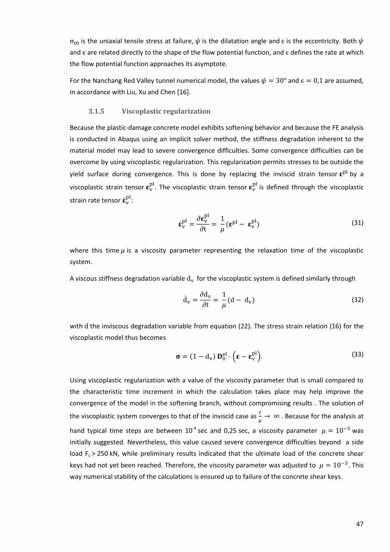
47

is the uniaxial tensile stress at failure, is the dilatation angle and is the eccentricity. Both

and are related directly to the shape of the flow potential function, and defines the rate at which

the flow potential function approaches its asymptote.

For the Nanchang Red Valley tunnel numerical model, the values and are assumed,

in accordance with Liu, Xu and Chen [16].

3.1.5 Viscoplastic regularization

Because the plastic-damage concrete model exhibits softening behavior and because the FE analysis

is conducted in Abaqus using an implicit solver method, the stiffness degradation inherent to the

material model may lead to severe convergence difficulties. Some convergence difficulties can be

overcome by using viscoplastic regularization. This regularization permits stresses to be outside the

yield surface during convergence. This is done by replacing the inviscid strain tensor by a

viscoplastic strain tensor

. The viscoplastic strain tensor

is defined through the viscoplastic

strain rate tensor

:

(31)

where this time is a viscosity parameter representing the relaxation time of the viscoplastic

system.

A viscous stiffness degradation variable for the viscoplastic system is defined similarly through

(32)

with the inviscous degradation variable from equation (22). The stress strain relation (16) for the

viscoplastic model thus becomes

(33)

Using viscoplastic regularization with a value of the viscosity parameter that is small compared to

the characteristic time increment in which the calculation takes place may help improve the

convergence of the model in the softening branch, without compromising results . The solution of

the viscoplastic system converges to that of the inviscid case as

. Because for the analysis at

hand typical time steps are between 10-4 sec and 0,25 sec, a viscosity parameter was

initially suggested. Nevertheless, this value caused severe convergence difficulties beyond a side

load Fs > 250 kN, while preliminary results indicated that the ultimate load of the concrete shear

keys had not yet been reached. Therefore, the viscosity parameter was adjusted to . This

way numerical stability of the calculations is ensured up to failure of the concrete shear keys.

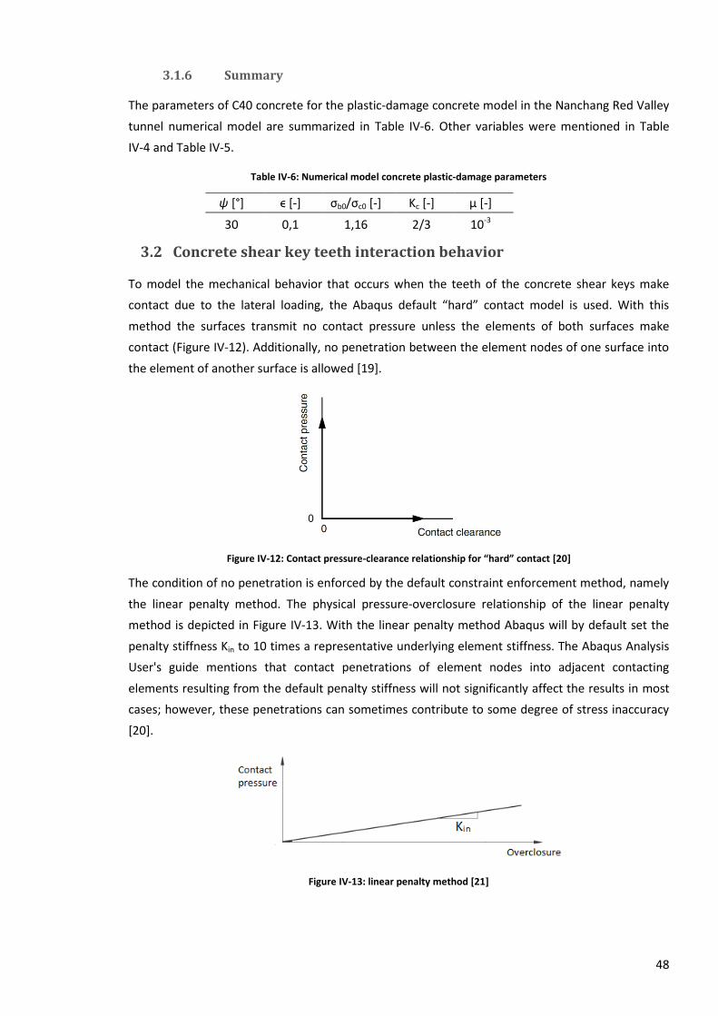
48

3.1.6 Summary

The parameters of C40 concrete for the plastic-damage concrete model in the Nanchang Red Valley

tunnel numerical model are summarized in Table IV-6. Other variables were mentioned in Table

IV-4 and Table IV-5.

Table IV-6: Numerical model concrete plastic-damage parameters

ψ [°] ϵ [-] σb0/σc0 [-] Kc [-] μ [-]

30 0,1 1,16 2/3 10-3

3.2 Concrete shear key teeth interaction behavior

To model the mechanical behavior that occurs when the teeth of the concrete shear keys make

contact due to the lateral loading, the Abaqus default “hard” contact model is used. With this

method the surfaces transmit no contact pressure unless the elements of both surfaces make

contact (Figure IV-12). Additionally, no penetration between the element nodes of one surface into

the element of another surface is allowed [19].

Figure IV-12: Contact pressure-clearance relationship for “hard” contact [20]

The condition of no penetration is enforced by the default constraint enforcement method, namely

the linear penalty method. The physical pressure-overclosure relationship of the linear penalty

method is depicted in Figure IV-13. With the linear penalty method Abaqus will by default set the

penalty stiffness Kin to 10 times a representative underlying element stiffness. The Abaqus Analysis

User's guide mentions that contact penetrations of element nodes into adjacent contacting

elements resulting from the default penalty stiffness will not significantly affect the results in most

cases; however, these penetrations can sometimes contribute to some degree of stress inaccuracy

[20].

Figure IV-13: linear penalty method [21]

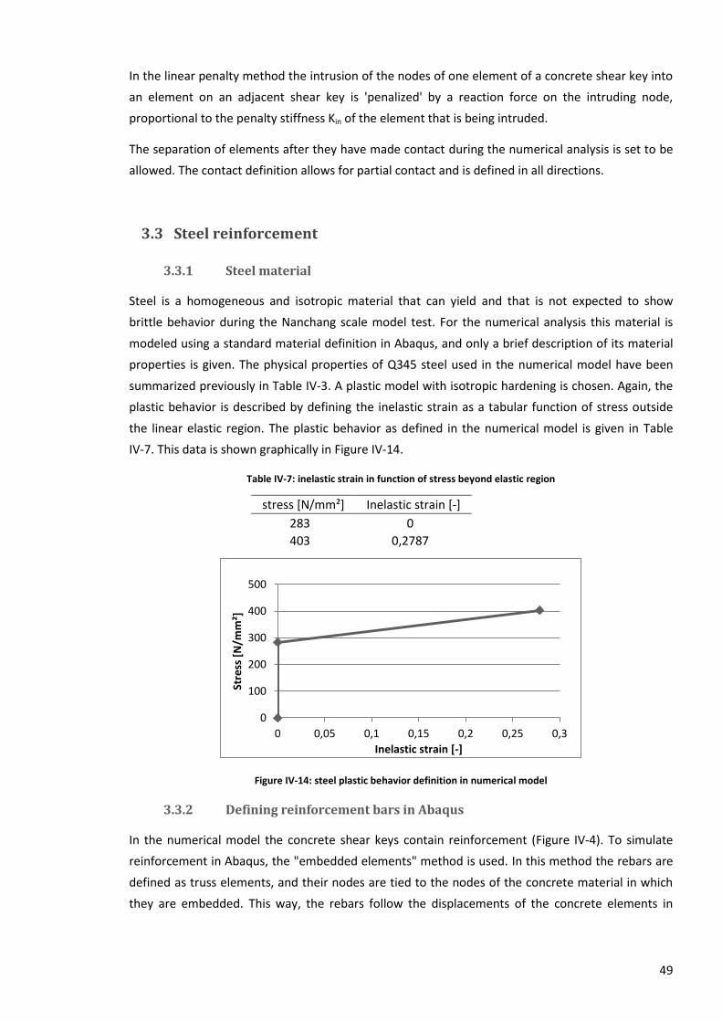
49

In the linear penalty method the intrusion of the nodes of one element of a concrete shear key into

an element on an adjacent shear key is 'penalized' by a reaction force on the intruding node,

proportional to the penalty stiffness Kin of the element that is being intruded.

The separation of elements after they have made contact during the numerical analysis is set to be

allowed. The contact definition allows for partial contact and is defined in all directions.

3.3 Steel reinforcement

3.3.1 Steel material

Steel is a homogeneous and isotropic material that can yield and that is not expected to show

brittle behavior during the Nanchang scale model test. For the numerical analysis this material is

modeled using a standard material definition in Abaqus, and only a brief description of its material

properties is given. The physical properties of Q345 steel used in the numerical model have been

summarized previously in Table IV-3. A plastic model with isotropic hardening is chosen. Again, the

plastic behavior is described by defining the inelastic strain as a tabular function of stress outside

the linear elastic region. The plastic behavior as defined in the numerical model is given in Table

IV-7. This data is shown graphically in Figure IV-14.

Table IV-7: inelastic strain in function of stress beyond elastic region

stress [N/mm²] Inelastic strain [-]

283 0

403 0,2787

Figure IV-14: steel plastic behavior definition in numerical model

3.3.2 Defining reinforcement bars in Abaqus

In the numerical model the concrete shear keys contain reinforcement (Figure IV-4). To simulate

reinforcement in Abaqus, the "embedded elements" method is used. In this method the rebars are

defined as truss elements, and their nodes are tied to the nodes of the concrete material in which

they are embedded. This way, the rebars follow the displacements of the concrete elements in

0

100

200

300

400

500

0 0,05 0,1 0,15 0,2 0,25 0,3

Stre

ss [

N/m

m²]

Inelastic strain [-]

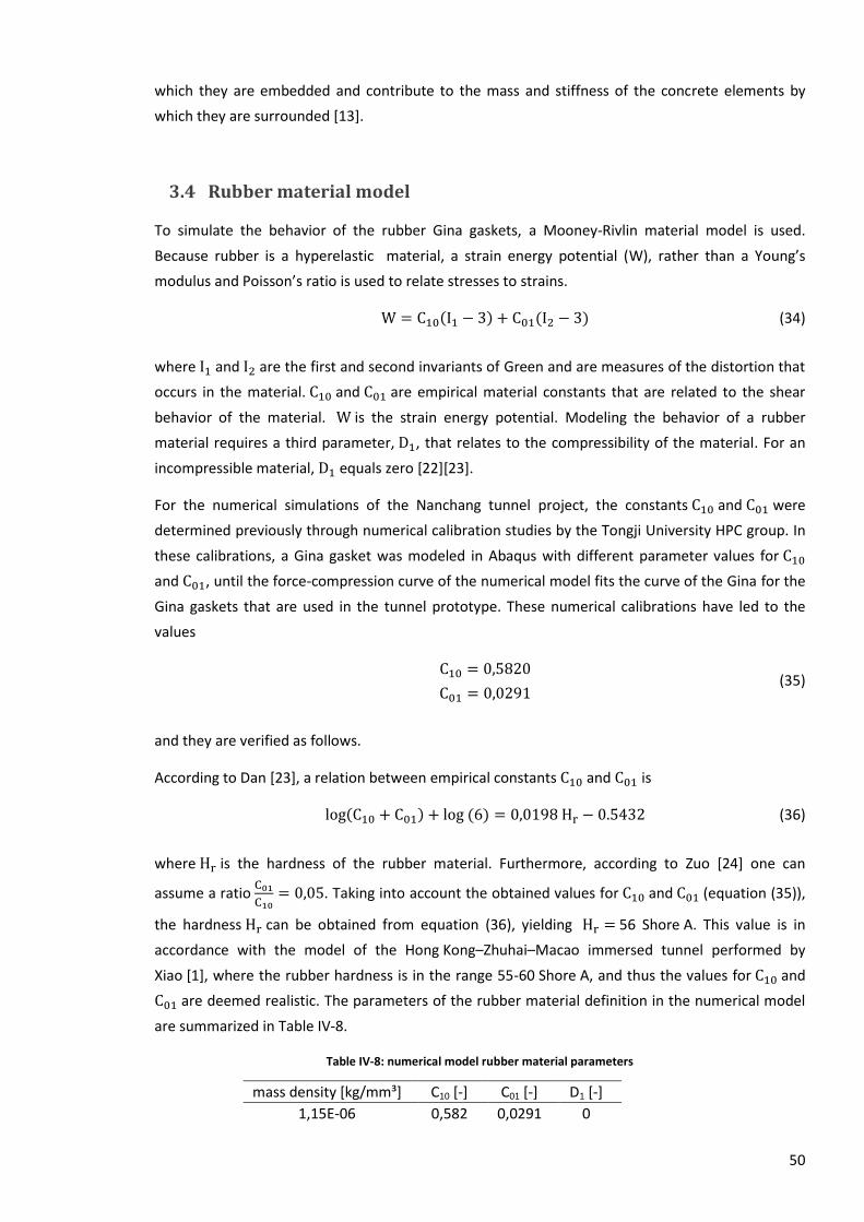
50

which they are embedded and contribute to the mass and stiffness of the concrete elements by

which they are surrounded [13].

3.4 Rubber material model

To simulate the behavior of the rubber Gina gaskets, a Mooney-Rivlin material model is used.

Because rubber is a hyperelastic material, a strain energy potential (W), rather than a Young’s

modulus and Poisson’s ratio is used to relate stresses to strains.

(34)

where and are the first and second invariants of Green and are measures of the distortion that

occurs in the material. and are empirical material constants that are related to the shear

behavior of the material. is the strain energy potential. Modeling the behavior of a rubber

material requires a third parameter, , that relates to the compressibility of the material. For an

incompressible material, equals zero [22][23].

For the numerical simulations of the Nanchang tunnel project, the constants and were

determined previously through numerical calibration studies by the Tongji University HPC group. In

these calibrations, a Gina gasket was modeled in Abaqus with different parameter values for

and , until the force-compression curve of the numerical model fits the curve of the Gina for the

Gina gaskets that are used in the tunnel prototype. These numerical calibrations have led to the

values

(35)

and they are verified as follows.

According to Dan [23], a relation between empirical constants and is

(36)

where is the hardness of the rubber material. Furthermore, according to Zuo [24] one can

assume a ratio

. Taking into account the obtained values for and (equation (35)),

the hardness can be obtained from equation (36), yielding 56 Shore A. This value is in

accordance with the model of the Hong Kong–Zhuhai–Macao immersed tunnel performed by

Xiao [1], where the rubber hardness is in the range 55-60 Shore A, and thus the values for and

are deemed realistic. The parameters of the rubber material definition in the numerical model

are summarized in Table IV-8.

Table IV-8: numerical model rubber material parameters

mass density [kg/mm³] C10 [-] C01 [-] D1 [-]

1,15E-06 0,582 0,0291 0

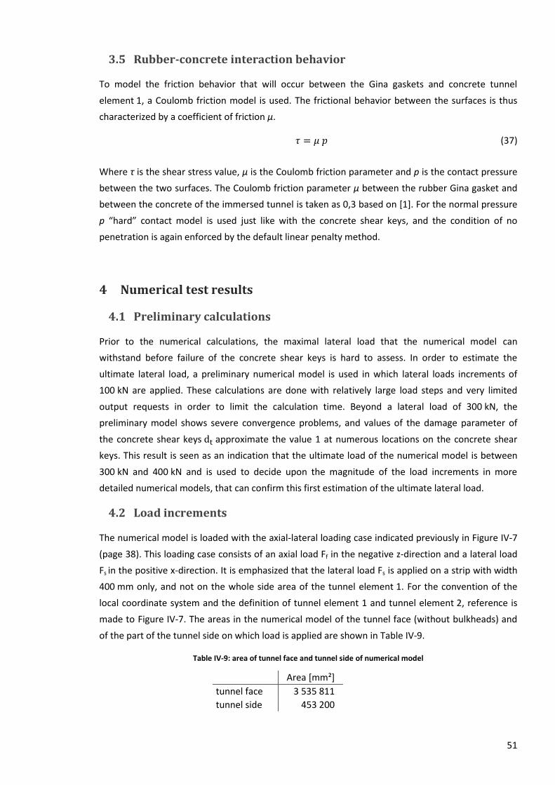
51

3.5 Rubber-concrete interaction behavior

To model the friction behavior that will occur between the Gina gaskets and concrete tunnel

element 1, a Coulomb friction model is used. The frictional behavior between the surfaces is thus

characterized by a coefficient of friction μ.

(37)

Where τ is the shear stress value, μ is the Coulomb friction parameter and p is the contact pressure

between the two surfaces. The Coulomb friction parameter μ between the rubber Gina gasket and

between the concrete of the immersed tunnel is taken as 0,3 based on [1]. For the normal pressure

p “hard” contact model is used just like with the concrete shear keys, and the condition of no

penetration is again enforced by the default linear penalty method.

4 Numerical test results

4.1 Preliminary calculations

Prior to the numerical calculations, the maximal lateral load that the numerical model can

withstand before failure of the concrete shear keys is hard to assess. In order to estimate the

ultimate lateral load, a preliminary numerical model is used in which lateral loads increments of

100 kN are applied. These calculations are done with relatively large load steps and very limited

output requests in order to limit the calculation time. Beyond a lateral load of 300 kN, the

preliminary model shows severe convergence problems, and values of the damage parameter of

the concrete shear keys approximate the value 1 at numerous locations on the concrete shear

keys. This result is seen as an indication that the ultimate load of the numerical model is between

300 kN and 400 kN and is used to decide upon the magnitude of the load increments in more

detailed numerical models, that can confirm this first estimation of the ultimate lateral load.

4.2 Load increments

The numerical model is loaded with the axial-lateral loading case indicated previously in Figure IV-7

(page 38). This loading case consists of an axial load Ff in the negative z-direction and a lateral load

Fs in the positive x-direction. It is emphasized that the lateral load Fs is applied on a strip with width

400 mm only, and not on the whole side area of the tunnel element 1. For the convention of the

local coordinate system and the definition of tunnel element 1 and tunnel element 2, reference is

made to Figure IV-7. The areas in the numerical model of the tunnel face (without bulkheads) and

of the part of the tunnel side on which load is applied are shown in Table IV-9.

Table IV-9: area of tunnel face and tunnel side of numerical model

Area [mm²]

tunnel face 3 535 811

tunnel side 453 200

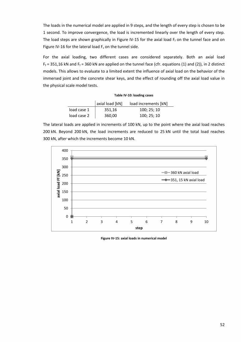
52

The loads in the numerical model are applied in 9 steps, and the length of every step is chosen to be

1 second. To improve convergence, the load is incremented linearly over the length of every step.

The load steps are shown graphically in Figure IV-15 for the axial load Ff on the tunnel face and on

Figure IV-16 for the lateral load Fs on the tunnel side.

For the axial loading, two different cases are considered separately. Both an axial load

Ff = 351,16 kN and Ff = 360 kN are applied on the tunnel face (cfr. equations (1) and (2)), in 2 distinct

models. This allows to evaluate to a limited extent the influence of axial load on the behavior of the

immersed joint and the concrete shear keys, and the effect of rounding off the axial load value in

the physical scale model tests.

Table IV-10: loading cases

axial load [kN] load increments [kN]

load case 1 351,16 100; 25; 10

load case 2 360,00 100; 25; 10

The lateral loads are applied in increments of 100 kN, up to the point where the axial load reaches

200 kN. Beyond 200 kN, the load increments are reduced to 25 kN until the total load reaches

300 kN, after which the increments become 10 kN.

Figure IV-15: axial loads in numerical model

0

50

100

150

200

250

300

350

400

1 2 3 4 5 6 7 8 9 10

axia

l lo

ad F

f [k

N]

step

360 kN axial load

351, 15 kN axial load

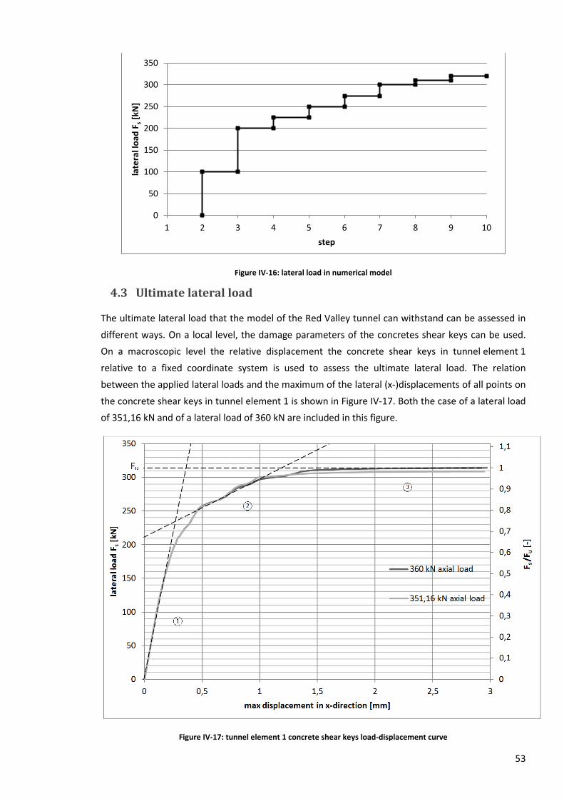
53

Figure IV-16: lateral load in numerical model

4.3 Ultimate lateral load

The ultimate lateral load that the model of the Red Valley tunnel can withstand can be assessed in

different ways. On a local level, the damage parameters of the concretes shear keys can be used.

On a macroscopic level the relative displacement the concrete shear keys in tunnel element 1

relative to a fixed coordinate system is used to assess the ultimate lateral load. The relation

between the applied lateral loads and the maximum of the lateral (x-)displacements of all points on

the concrete shear keys in tunnel element 1 is shown in Figure IV-17. Both the case of a lateral load

of 351,16 kN and of a lateral load of 360 kN are included in this figure.

Figure IV-17: tunnel element 1 concrete shear keys load-displacement curve

0

50

100

150

200

250

300

350

1 2 3 4 5 6 7 8 9 10

late

ral l

oad

Fs

[kN

]

step

54

For both values of the axial load, the load-displacement curves are identical up to a lateral load of

250 kN, and a clear linear elastic behavior is present at a lateral load up to about 200 kN (region ○1

in Figure IV-17), after which the stiffness degrades significantly. For the 360 kN axial loading case,

the displacement is 0,105 mm at lateral load of 100 kN, from which the initial lateral stiffness of the

joint can be obtained as

(38)

At a lateral load of 210 kN, a first relatively sudden loss of lateral stiffness seems to occur. A second

and more sudden increase in lateral displacement occurs just after the lateral load of 250 kN. At this

stage the initial lateral stiffness has degraded significantly (region ○2 ). Between the application of

the lateral loads of 250 kN and 300 kN, the stiffness has degraded to approximately

(39)

These results show that the stiffness of the joint is reduced by 92,5% when the lateral load reaches

two thirds of the ultimate value at failure Fu.

Beyond a lateral load of 300 kN (region ○3 ), the maxima of the displacements of all points on the

shear keys in tunnel element 1 becomes very large compared to the applied lateral load increments.

At a lateral load of 314 kN the load-displacement relation becomes asymptotical, indicating

complete loss of stiffness ( = 0 kN/mm) and thus failure of the concrete shear keys. Under an

axial load of 360 kN, the ultimate lateral load that can be applied to the model, resulting in

complete damage of the concrete shear keys is thus estimated to be

(40)

The influence of the two slightly different axial loads is only significant to a limited extent in regions

○2 and ○3 of the load-displacement curve. Sudden decrease of stiffness is inherent to damage

behavior of brittle materials, which clearly occurs in region ○2 of the load-displacement curve. In

that part the load-displacement curves of load case 1 and load case 2 are no longer identical, as the

sudden decrease in stiffness occurs at different lateral loads. This indicates that the axial

compression load does have an influence on the load-displacement behavior of the immersed joint.

The fact that the ultimate load for loading case 2 is larger than for loading case 1 is explained by the

fact that under larger compression loads, the Gina gaskets take up additional loads through friction

between concrete element 1 and the Gina gaskets according to Coulomb's friction law.

4.4 Concrete shear key damage

The results of the numerical model are used to predict the damage behavior of the concrete shear

keys. Damage is defined as a change in material properties that adversely affects the performance

(in this case the stiffness) of the material, and in this case cracking is considered to be a

manifestation of damage. According to Lubliner [15], cracking initiates at a point where the maximal

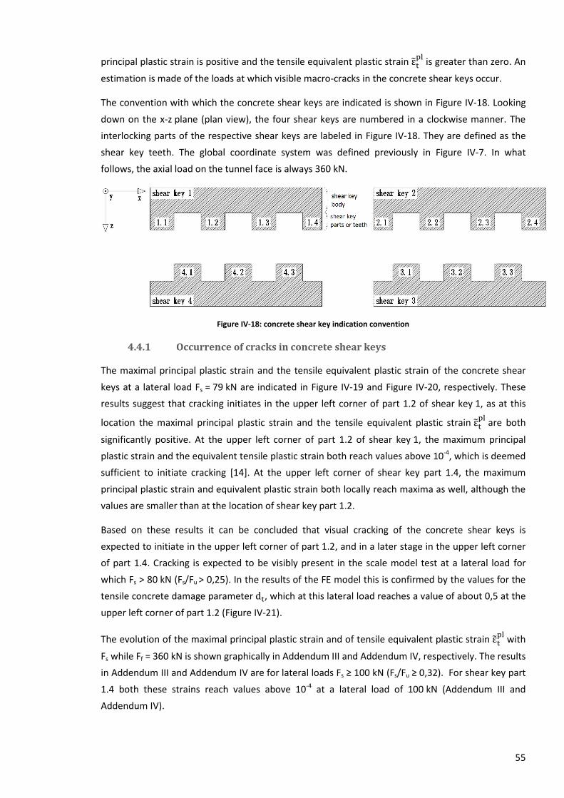
55

principal plastic strain is positive and the tensile equivalent plastic strain

is greater than zero. An

estimation is made of the loads at which visible macro-cracks in the concrete shear keys occur.

The convention with which the concrete shear keys are indicated is shown in Figure IV-18. Looking

down on the x-z plane (plan view), the four shear keys are numbered in a clockwise manner. The

interlocking parts of the respective shear keys are labeled in Figure IV-18. They are defined as the

shear key teeth. The global coordinate system was defined previously in Figure IV-7. In what

follows, the axial load on the tunnel face is always 360 kN.

Figure IV-18: concrete shear key indication convention

4.4.1 Occurrence of cracks in concrete shear keys

The maximal principal plastic strain and the tensile equivalent plastic strain of the concrete shear

keys at a lateral load Fs = 79 kN are indicated in Figure IV-19 and Figure IV-20, respectively. These

results suggest that cracking initiates in the upper left corner of part 1.2 of shear key 1, as at this

location the maximal principal plastic strain and the tensile equivalent plastic strain

are both

significantly positive. At the upper left corner of part 1.2 of shear key 1, the maximum principal

plastic strain and the equivalent tensile plastic strain both reach values above 10-4, which is deemed

sufficient to initiate cracking [14]. At the upper left corner of shear key part 1.4, the maximum

principal plastic strain and equivalent plastic strain both locally reach maxima as well, although the

values are smaller than at the location of shear key part 1.2.

Based on these results it can be concluded that visual cracking of the concrete shear keys is

expected to initiate in the upper left corner of part 1.2, and in a later stage in the upper left corner

of part 1.4. Cracking is expected to be visibly present in the scale model test at a lateral load for

which Fs > 80 kN (Fs/Fu > 0,25). In the results of the FE model this is confirmed by the values for the

tensile concrete damage parameter , which at this lateral load reaches a value of about 0,5 at the

upper left corner of part 1.2 (Figure IV-21).

The evolution of the maximal principal plastic strain and of tensile equivalent plastic strain

with

Fs while Ff = 360 kN is shown graphically in Addendum III and Addendum IV, respectively. The results

in Addendum III and Addendum IV are for lateral loads Fs ≥ 100 kN (Fs/Fu ≥ 0,32). For shear key part

1.4 both these strains reach values above 10-4 at a lateral load of 100 kN (Addendum III and

Addendum IV).

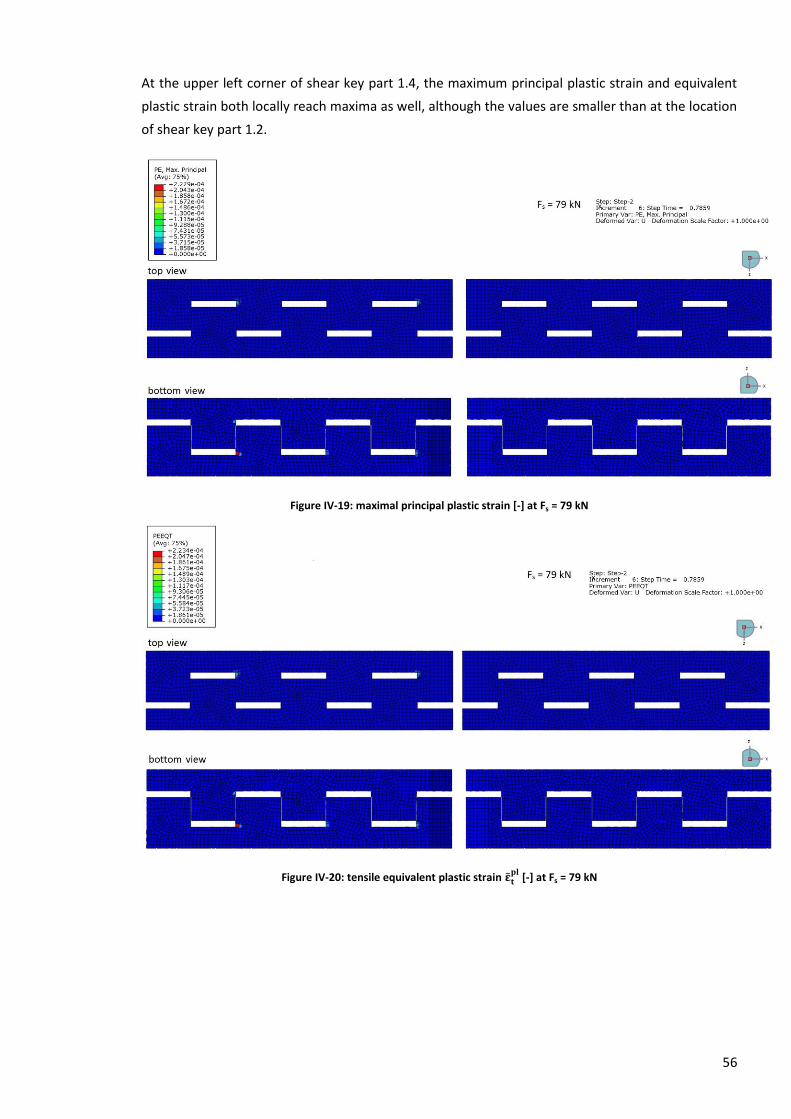
56

At the upper left corner of shear key part 1.4, the maximum principal plastic strain and equivalent

plastic strain both locally reach maxima as well, although the values are smaller than at the location

of shear key part 1.2.

Figure IV-19: maximal principal plastic strain [-] at Fs = 79 kN

Figure IV-20: tensile equivalent plastic strain

[-] at Fs = 79 kN

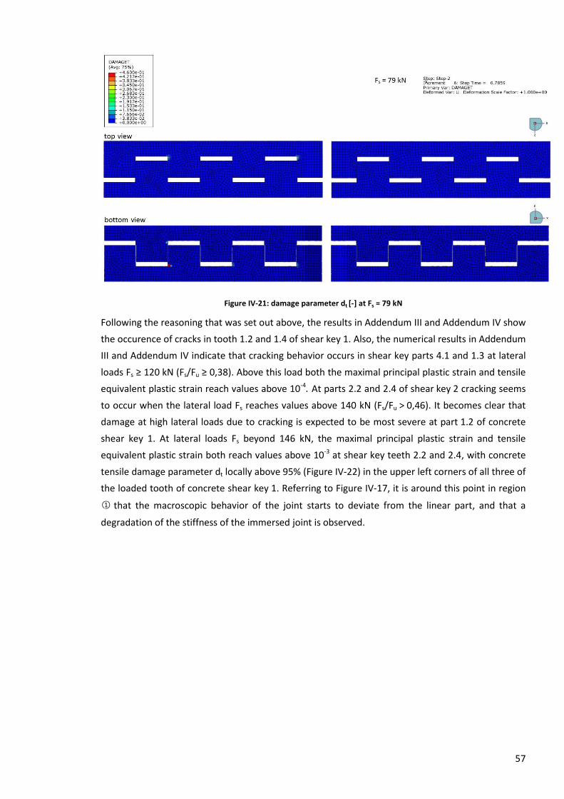
57

Figure IV-21: damage parameter dt [-] at Fs = 79 kN

Following the reasoning that was set out above, the results in Addendum III and Addendum IV show

the occurence of cracks in tooth 1.2 and 1.4 of shear key 1. Also, the numerical results in Addendum

III and Addendum IV indicate that cracking behavior occurs in shear key parts 4.1 and 1.3 at lateral

loads Fs ≥ 120 kN (Fs/Fu ≥ 0,38). Above this load both the maximal principal plastic strain and tensile

equivalent plastic strain reach values above 10-4. At parts 2.2 and 2.4 of shear key 2 cracking seems

to occur when the lateral load Fs reaches values above 140 kN (Fs/Fu > 0,46). It becomes clear that

damage at high lateral loads due to cracking is expected to be most severe at part 1.2 of concrete

shear key 1. At lateral loads Fs beyond 146 kN, the maximal principal plastic strain and tensile

equivalent plastic strain both reach values above 10-3 at shear key teeth 2.2 and 2.4, with concrete

tensile damage parameter dt locally above 95% (Figure IV-22) in the upper left corners of all three of

the loaded tooth of concrete shear key 1. Referring to Figure IV-17, it is around this point in region

○1 that the macroscopic behavior of the joint starts to deviate from the linear part, and that a

degradation of the stiffness of the immersed joint is observed.

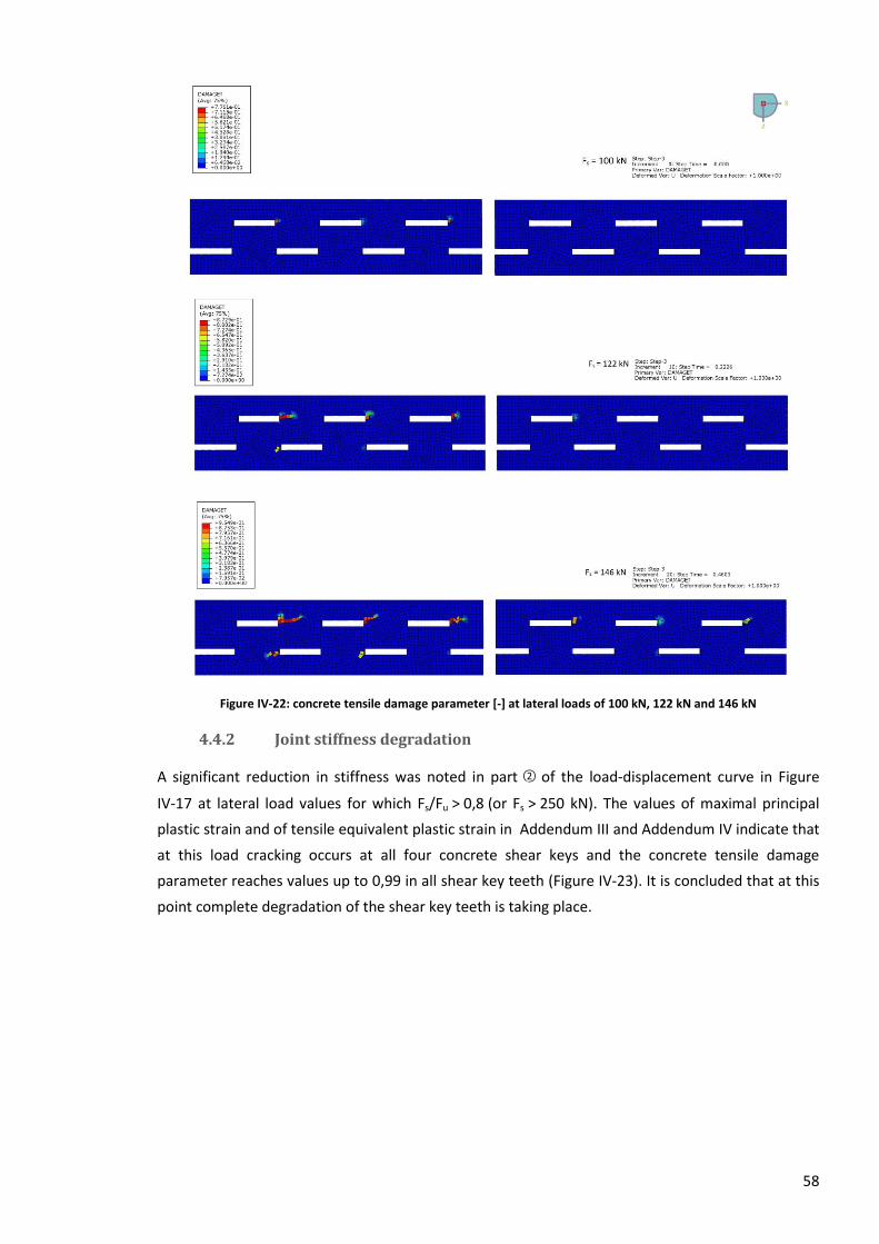
58

Figure IV-22: concrete tensile damage parameter [-] at lateral loads of 100 kN, 122 kN and 146 kN

4.4.2 Joint stiffness degradation

A significant reduction in stiffness was noted in part ○2 of the load-displacement curve in Figure

IV-17 at lateral load values for which Fs/Fu > 0,8 (or Fs > 250 kN). The values of maximal principal

plastic strain and of tensile equivalent plastic strain in Addendum III and Addendum IV indicate that

at this load cracking occurs at all four concrete shear keys and the concrete tensile damage

parameter reaches values up to 0,99 in all shear key teeth (Figure IV-23). It is concluded that at this

point complete degradation of the shear key teeth is taking place.

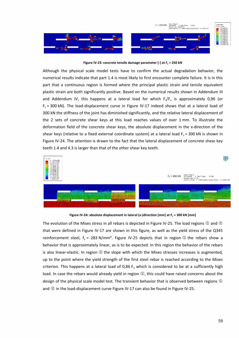
59

Figure IV-23: concrete tensile damage parameter [-] at Fs = 250 kN

Although the physical scale model tests have to confirm the actual degradation behavior, the

numerical results indicate that part 1.4 is most likely to first encounter complete failure. It is in this

part that a continuous region is formed where the principal plastic strain and tensile equivalent

plastic strain are both significantly positive. Based on the numerical results shown in Addendum III

and Addendum IV, this happens at a lateral load for which Fs/Fu is approximately 0,96 (or

Fs = 300 kN). The load-displacement curve in Figure IV-17 indeed shows that at a lateral load of

300 kN the stiffness of the joint has diminished significantly, and the relative lateral displacement of

the 2 sets of concrete shear keys at this load reaches values of over 1 mm. To illustrate the

deformation field of the concrete shear keys, the absolute displacement in the x-direction of the

shear keys (relative to a fixed external coordinate system) at a lateral load Fs = 300 kN is shown in

Figure IV-24. The attention is drawn to the fact that the lateral displacement of concrete shear key

teeth 1.4 and 4.3 is larger than that of the other shear key teeth.

Figure IV-24: absolute displacement in lateral (x-)direction [mm] at Fs = 300 kN [mm]

The evolution of the Mises stress in all rebars is depicted in Figure IV-25. The load regions ○1 and ○2

that were defined in Figure IV-17 are shown in this figure, as well as the yield stress of the Q345

reinforcement steel, fy = 283 N/mm². Figure IV-25 depicts that in region ○1 the rebars show a

behavior that is approximately linear, as is to be expected. In this region the behavior of the rebars

is also linear-elastic. In region ○2 the slope with which the Mises stresses increases is augmented,

up to the point where the yield strength of the first steel rebar is reached according to the Mises

criterion. This happens at a lateral load of 0,86 Fu which is considered to be at a sufficiently high

load. In case the rebars would already yield in region ○1 , this could have raised concerns about the

design of the physical scale model test. The transient behavior that is observed between regions ○1

and ○2 in the load-displacement curve Figure IV-17 can also be found in Figure IV-25.

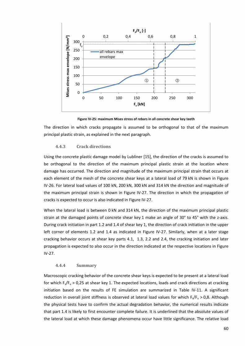
60

Figure IV-25: maximum Mises stress of rebars in all concrete shear key teeth

The direction in which cracks propagate is assumed to be orthogonal to that of the maximum

principal plastic strain, as explained in the next paragraph.

4.4.3 Crack directions

Using the concrete plastic damage model by Lubliner [15], the direction of the cracks is assumed to

be orthogonal to the direction of the maximum principal plastic strain at the location where

damage has occurred. The direction and magnitude of the maximum principal strain that occurs at

each element of the mesh of the concrete shear keys at a lateral load of 79 kN is shown in Figure

IV-26. For lateral load values of 100 kN, 200 kN, 300 kN and 314 kN the direction and magnitude of

the maximum principal strain is shown in Figure IV-27. The direction in which the propagation of

cracks is expected to occur is also indicated in Figure IV-27.

When the lateral load is between 0 kN and 314 kN, the direction of the maximum principal plastic

strain at the damaged points of concrete shear key 1 make an angle of 30° to 45° with the z-axis.

During crack initiation in part 1.2 and 1.4 of shear key 1, the direction of crack initiation in the upper

left corner of elements 1.2 and 1.4 as indicated in Figure IV-27. Similarly, when at a later stage

cracking behavior occurs at shear key parts 4.1, 1.3, 2.2 and 2.4, the cracking initiation and later

propagation is expected to also occur in the direction indicated at the respective locations in Figure

IV-27.

4.4.4 Summary

Macroscopic cracking behavior of the concrete shear keys is expected to be present at a lateral load

for which Fs/Fu > 0,25 at shear key 1. The expected locations, loads and crack directions at cracking

initiation based on the results of FE simulation are summarized in Table IV-11. A significant

reduction in overall joint stiffness is observed at lateral load values for which Fs/Fu > 0,8. Although

the physical tests have to confirm the actual degradation behavior, the numerical results indicate

that part 1.4 is likely to first encounter complete failure. It is underlined that the absolute values of

the lateral load at which these damage phenomena occur have little significance. The relative load

0 0,2 0,4 0,6 0,8 1

0

50

100

150

200

250

300

0 50 100 150 200 250 300

Fs/Fu [-]

Mis

es

stre

ss m

ax e

nve

lop

e [

N/m

m²]

Fs [kN]

all rebars max envelope

fy

○1 ○2

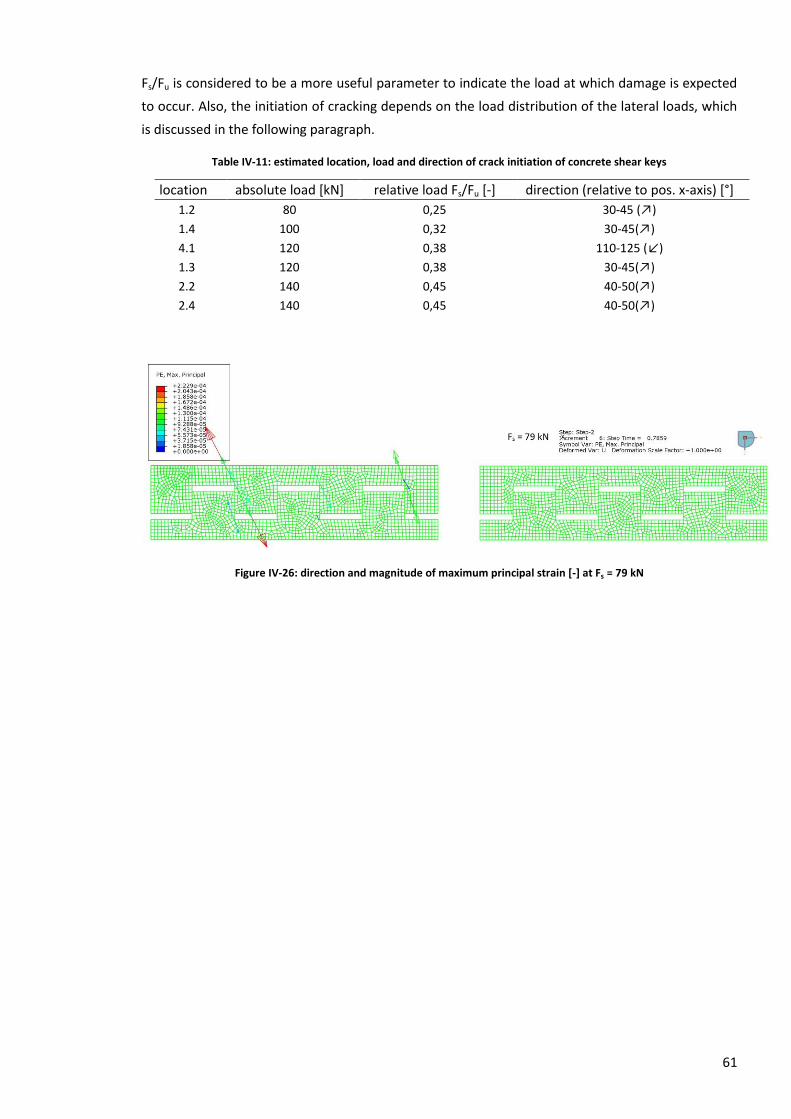
61

Fs/Fu is considered to be a more useful parameter to indicate the load at which damage is expected

to occur. Also, the initiation of cracking depends on the load distribution of the lateral loads, which

is discussed in the following paragraph.

Table IV-11: estimated location, load and direction of crack initiation of concrete shear keys

location absolute load [kN] relative load Fs/Fu [-] direction (relative to pos. x-axis) [°]

1.2 80 0,25 30-45 (↗)

1.4 100 0,32 30-45(↗)

4.1 120 0,38 110-125 (↙)

1.3 120 0,38 30-45(↗)

2.2 140 0,45 40-50(↗)

2.4 140 0,45 40-50(↗)

Figure IV-26: direction and magnitude of maximum principal strain [-] at Fs = 79 kN

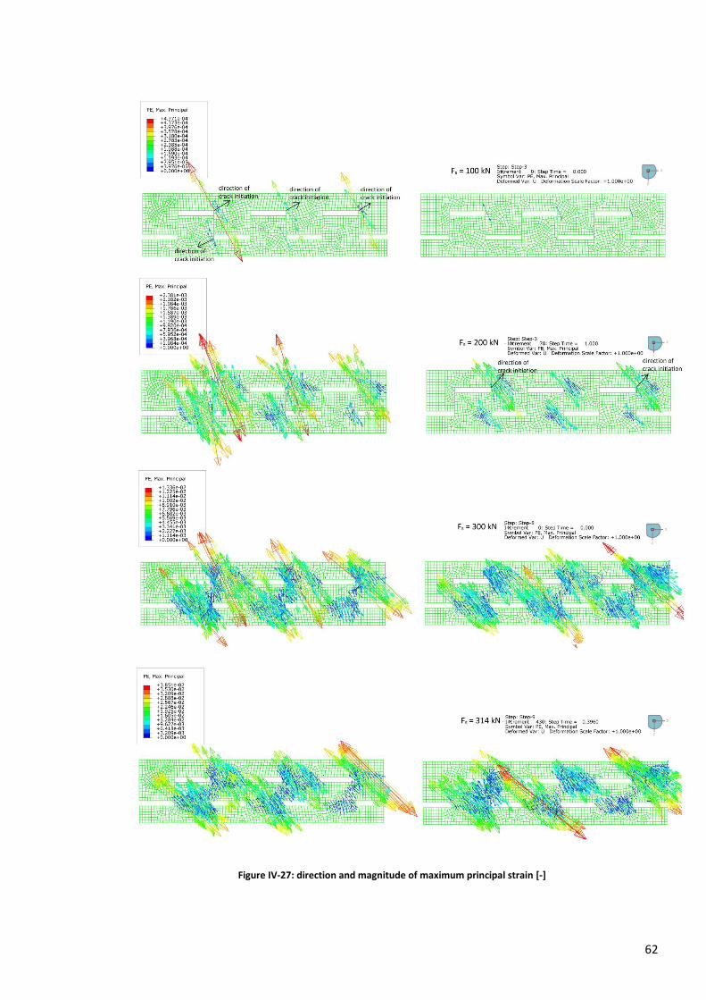
62

Figure IV-27: direction and magnitude of maximum principal strain [-]

63

4.5 Load distribution

In the analysis of the structural behavior of the concrete shear keys, one of the issues of interest is

the way the applied external forces are distributed as internal forces in the joint of the immersed

tunnel. In both the physical and the numerical model of the Nanchang Red Valley tunnel, the

applied lateral forces are expected to be carried primarily by the concrete shear keys, and to a less

extent by the Gina gasket and by the steel shear keys. In the following paragraphs, the load

distribution in the immersed joint is assessed.

4.5.1 Influence of steel shear keys

The structural members in the immersed joint that can transfer loads between the two tunnel

elements are hatched in Figure IV-28. They include the concrete shear keys, the steel shear keys and

the Gina gaskets. It was mentioned previously that the influence of the vertical steel shear keys on

the stress distribution under lateral loads in the immersed joint is assumed to be negligible, and the

steel shear keys are even omitted from the numerical calculations completely. In the physical scale

model of the Nanchang Red Valley Tunnel, however, the steel shear keys are present. To assess

whether the omission of the steel shear keys in the numerical model can be justified, the vertical

displacement of the two tunnel elements relative to each other is discussed.

As long as the relative vertical displacement (i.e. the displacement in the y-direction) of the 2 tunnel

elements in the numerical model without steel shear keys at the location of the omitted steel shear

keys is small enough, the omission of the steel shear keys can be justified. In the case of small

vertical displacements, the steel shear keys only just make contact and do not transfer any forces,

because there is no friction between the outer steel plates. Also, because the vertical shear keys do

not exert reaction forces on one another they cannot deform, and interlocking of deformed parts of

the steel shear keys cannot contribute to the transfer of lateral forces between the two tunnel

elements. This explains why the relative vertical displacement of the two tunnel elements in the

numerical model without concrete shear keys is used to assess whether the omission of the steel

shear keys in the numerical model is justified.

The results of the numerical model indicate that the displacements in the vertical (y-)direction of

the model without steel shear key are at a maximum when the lateral load is at its maximum of

314 kN. The absolute displacements of tunnel elements 1 and 2 at this lateral load are shown in

Figure IV-29. These displacements are measured relative to a fixed coordinate system outside the

tunnel. The results depicted in this figure indicate that the relative displacement of the two tunnel

elements is smaller than 0,06 mm at all the locations where steel shear keys are attached to the

concrete elements. The numerical results also show that the rotation around the x-axis of the

tunnel elements is negligably small. This indicates that the steel shear keys will only just make

contact and thus will not contribute to the overall load transfer that occurs in the joints.

It can be argued that the forces transferred between the steel shear keys in the numerical model do

have significance in the sense that they represent a force transfer that is the result of the

deformation of the concrete elements and of the other structural elements under the applied

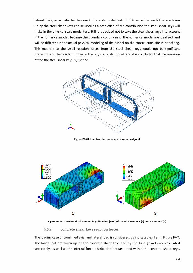
64

lateral loads, as will also be the case in the scale model tests. In this sense the loads that are taken

up by the steel shear keys can be used as a prediction of the contribution the steel shear keys will

make in the physical scale model test. Still it is decided not to take the steel shear keys into account

in the numerical model, because the boundary conditions of the numerical model are idealized, and

will be different in the actual physical modeling of the tunnel on the construction site in Nanchang.

This means that the small reaction forces from the steel shear keys would not be significant

predictions of the reaction forces in the physical scale model, and it is concluded that the omission

of the the steel shear keys is justified.

Figure IV-28: load transfer members in immersed joint

Figure IV-29: absolute displacement in y-direction [mm] of tunnel element 1 (a) and element 2 (b)

4.5.2 Concrete shear keys reaction forces

The loading case of combined axial and lateral load is considered, as indicated earlier in Figure IV-7.

The loads that are taken up by the concrete shear keys and by the Gina gaskets are calculated

separately, as well as the internal force distribution between and within the concrete shear keys.

65

The effect of the steel shear keys is neglected as explained in the above paragraph. The lateral loads

are expected to be taken up primarily by the concrete shear keys and to less extent by the Gina

gaskets. The results from the FE analysis will confirm this assumption.

When lateral load is applied on the side of tunnel element 1 (Figure IV-7), the vertical faces on the

side of the teeth of the concrete shear keys make contact, and contact pressures perpendicular to

these vertical faces occur. This results in a force transfer through the joint of the immersed tunnel.

Figure IV-30 shows contact pressures on the side of concrete shear keys 1 and 2. For all four the

concrete shear keys, the numerical results show a variation of the pressure over the contact area.

This variation is not considered to correspond to the real pressure variation that will occur in the

physical scale model test. In the physical scale model test, the teeth of the concrete shear keys are

separated by rubber supports (Figure IV-31). These rubber supports, that are not present in the

numerical model, will distribute the load that is transferred between the teeth, so that the exact

distribution of the contact stresses in the numerical model will not correspond to the distribution in

the physical scale model test.

Figure IV-30: contact pressures on side of concrete shear keys [N/mm²]

Figure IV-31: rubber supports in physical scale model

In Figure IV-18 the convention with which the concrete shear key parts are numbered was shown.

This figure is shown again below.

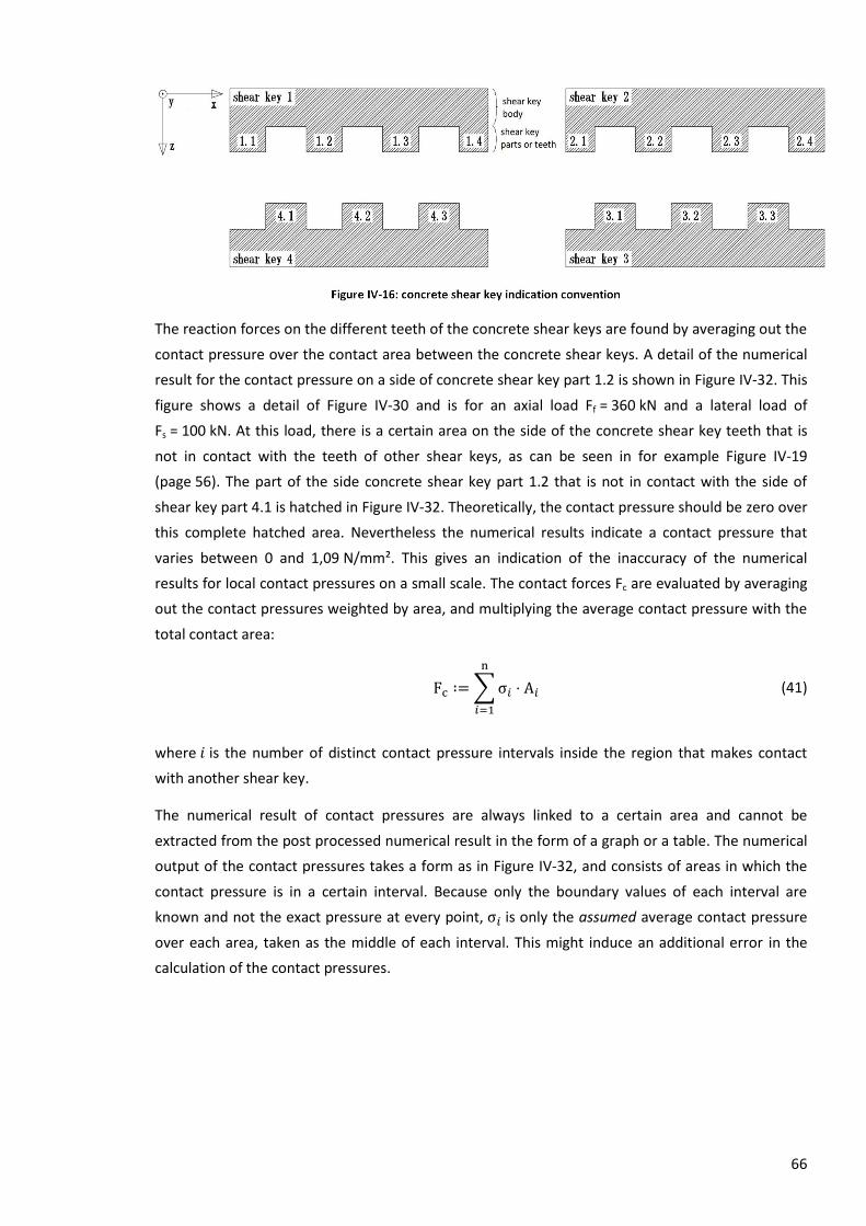
66

The reaction forces on the different teeth of the concrete shear keys are found by averaging out the

contact pressure over the contact area between the concrete shear keys. A detail of the numerical

result for the contact pressure on a side of concrete shear key part 1.2 is shown in Figure IV-32. This

figure shows a detail of Figure IV-30 and is for an axial load Ff = 360 kN and a lateral load of

Fs = 100 kN. At this load, there is a certain area on the side of the concrete shear key teeth that is

not in contact with the teeth of other shear keys, as can be seen in for example Figure IV-19

(page 56). The part of the side concrete shear key part 1.2 that is not in contact with the side of

shear key part 4.1 is hatched in Figure IV-32. Theoretically, the contact pressure should be zero over

this complete hatched area. Nevertheless the numerical results indicate a contact pressure that

varies between 0 and 1,09 N/mm². This gives an indication of the inaccuracy of the numerical

results for local contact pressures on a small scale. The contact forces Fc are evaluated by averaging

out the contact pressures weighted by area, and multiplying the average contact pressure with the

total contact area:

(41)

where is the number of distinct contact pressure intervals inside the region that makes contact

with another shear key.

The numerical result of contact pressures are always linked to a certain area and cannot be

extracted from the post processed numerical result in the form of a graph or a table. The numerical

output of the contact pressures takes a form as in Figure IV-32, and consists of areas in which the

contact pressure is in a certain interval. Because only the boundary values of each interval are

known and not the exact pressure at every point, is only the assumed average contact pressure

over each area, taken as the middle of each interval. This might induce an additional error in the

calculation of the contact pressures.

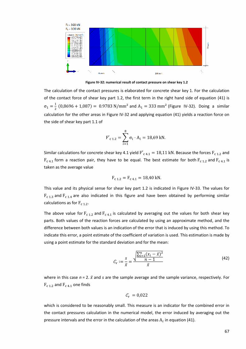
67

Figure IV-32: numerical result of contact pressure on shear key 1.2

The calculation of the contact pressures is elaborated for concrete shear key 1. For the calculation

of the contact force of shear key part 1.2, the first term in the right hand side of equation (41) is

and (Figure IV-32). Doing a similar

calculation for the other areas in Figure IV-32 and applying equation (41) yields a reaction force on

the side of shear key part 1.1 of

Similar calculations for concrete shear key 4.1 yield . Because the forces and

form a reaction pair, they have to be equal. The best estimate for both and is

taken as the average value

.

This value and its physical sense for shear key part 1.2 is indicated in Figure IV-33. The values for

and are also indicated in this figure and have been obtained by performing similar

calculations as for .

The above value for and is calculated by averaging out the values for both shear key

parts. Both values of the reaction forces are calculated by using an approximate method, and the

difference between both values is an indication of the error that is induced by using this method. To

indicate this error, a point estimate of the coefficient of variation is used. This estimation is made by

using a point estimate for the standard deviation and for the mean:

(42)

where in this case n = 2. and s are the sample average and the sample variance, respectively. For

and one finds

which is considered to be reasonably small. This measure is an indicator for the combined error in

the contact pressures calculation in the numerical model, the error induced by averaging out the

pressure intervals and the error in the calculation of the areas in equation (41).

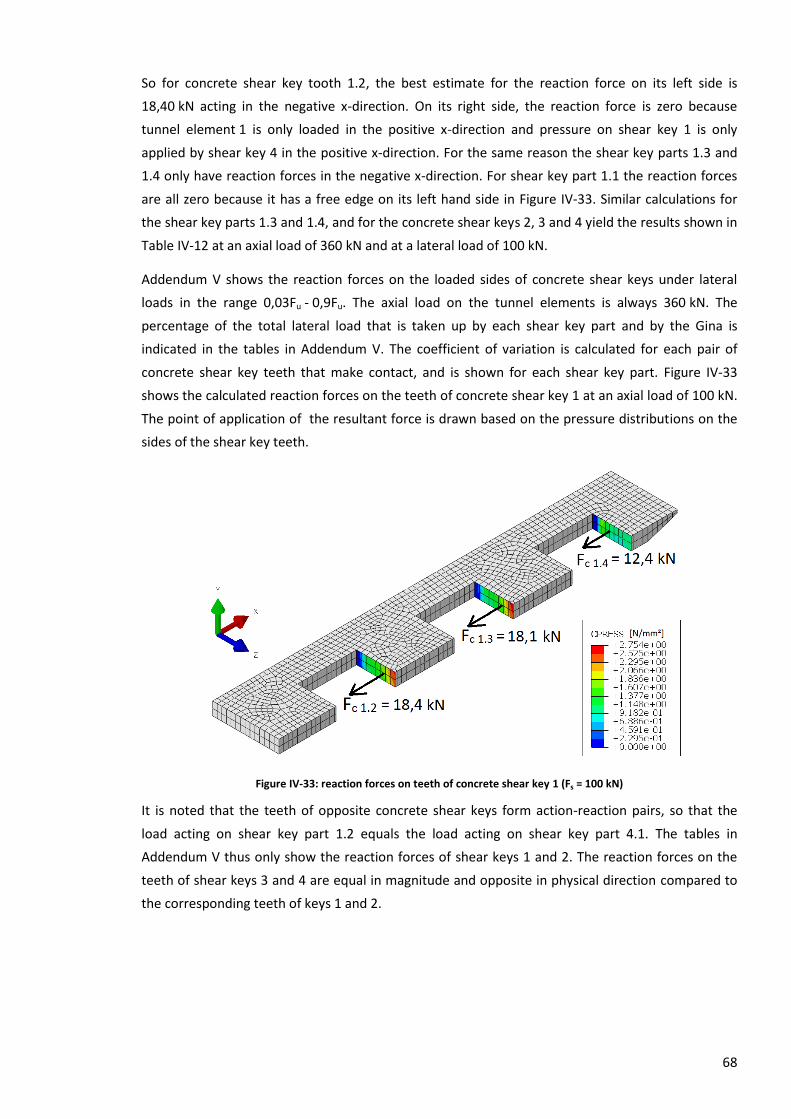
68

So for concrete shear key tooth 1.2, the best estimate for the reaction force on its left side is

18,40 kN acting in the negative x-direction. On its right side, the reaction force is zero because

tunnel element 1 is only loaded in the positive x-direction and pressure on shear key 1 is only

applied by shear key 4 in the positive x-direction. For the same reason the shear key parts 1.3 and

1.4 only have reaction forces in the negative x-direction. For shear key part 1.1 the reaction forces

are all zero because it has a free edge on its left hand side in Figure IV-33. Similar calculations for

the shear key parts 1.3 and 1.4, and for the concrete shear keys 2, 3 and 4 yield the results shown in

Table IV-12 at an axial load of 360 kN and at a lateral load of 100 kN.

Addendum V shows the reaction forces on the loaded sides of concrete shear keys under lateral

loads in the range 0,03Fu - 0,9Fu. The axial load on the tunnel elements is always 360 kN. The

percentage of the total lateral load that is taken up by each shear key part and by the Gina is

indicated in the tables in Addendum V. The coefficient of variation is calculated for each pair of

concrete shear key teeth that make contact, and is shown for each shear key part. Figure IV-33

shows the calculated reaction forces on the teeth of concrete shear key 1 at an axial load of 100 kN.

The point of application of the resultant force is drawn based on the pressure distributions on the

sides of the shear key teeth.

Figure IV-33: reaction forces on teeth of concrete shear key 1 (Fs = 100 kN)

It is noted that the teeth of opposite concrete shear keys form action-reaction pairs, so that the

load acting on shear key part 1.2 equals the load acting on shear key part 4.1. The tables in

Addendum V thus only show the reaction forces of shear keys 1 and 2. The reaction forces on the

teeth of shear keys 3 and 4 are equal in magnitude and opposite in physical direction compared to

the corresponding teeth of keys 1 and 2.

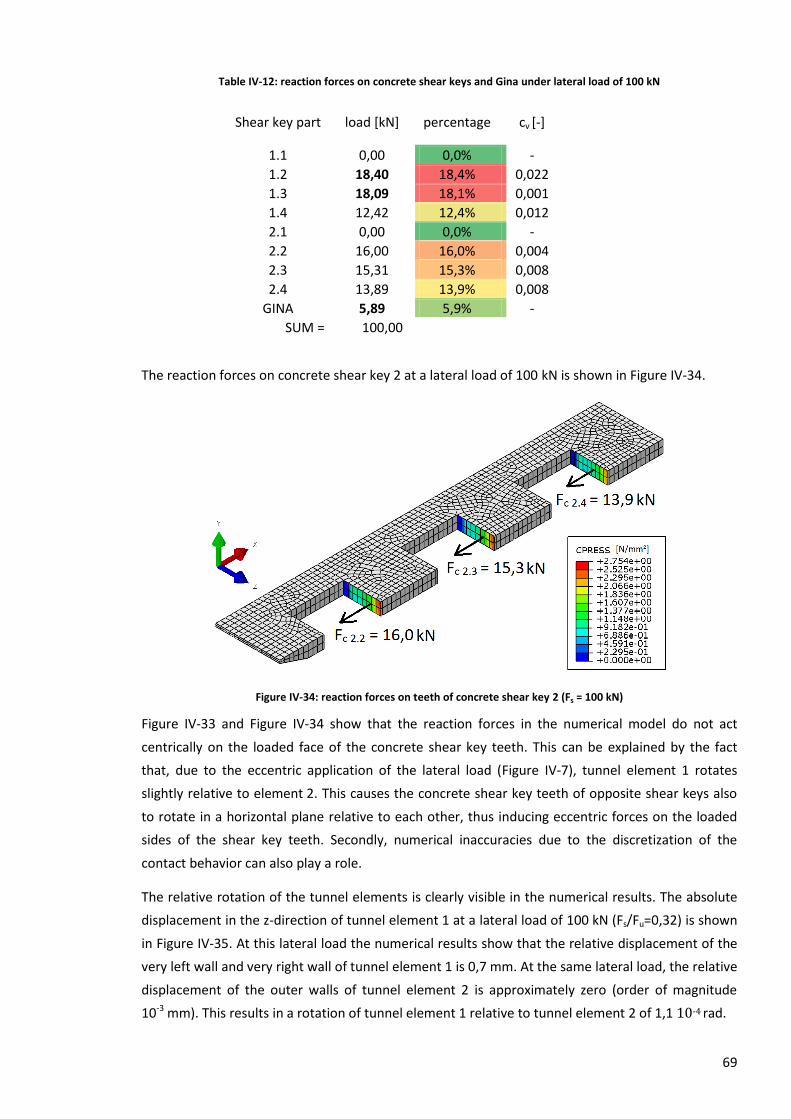
69

Table IV-12: reaction forces on concrete shear keys and Gina under lateral load of 100 kN

Shear key part load [kN] percentage cv [-]

1.1 0,00 0,0% -

1.2 18,40 18,4% 0,022

1.3 18,09 18,1% 0,001

1.4 12,42 12,4% 0,012

2.1 0,00 0,0% -

2.2 16,00 16,0% 0,004

2.3 15,31 15,3% 0,008

2.4 13,89 13,9% 0,008

GINA 5,89 5,9% -

SUM = 100,00

The reaction forces on concrete shear key 2 at a lateral load of 100 kN is shown in Figure IV-34.

Figure IV-34: reaction forces on teeth of concrete shear key 2 (Fs = 100 kN)

Figure IV-33 and Figure IV-34 show that the reaction forces in the numerical model do not act

centrically on the loaded face of the concrete shear key teeth. This can be explained by the fact

that, due to the eccentric application of the lateral load (Figure IV-7), tunnel element 1 rotates

slightly relative to element 2. This causes the concrete shear key teeth of opposite shear keys also

to rotate in a horizontal plane relative to each other, thus inducing eccentric forces on the loaded

sides of the shear key teeth. Secondly, numerical inaccuracies due to the discretization of the

contact behavior can also play a role.

The relative rotation of the tunnel elements is clearly visible in the numerical results. The absolute

displacement in the z-direction of tunnel element 1 at a lateral load of 100 kN (Fs/Fu=0,32) is shown

in Figure IV-35. At this lateral load the numerical results show that the relative displacement of the

very left wall and very right wall of tunnel element 1 is 0,7 mm. At the same lateral load, the relative

displacement of the outer walls of tunnel element 2 is approximately zero (order of magnitude

10-3 mm). This results in a rotation of tunnel element 1 relative to tunnel element 2 of 1,1 10-4 rad.

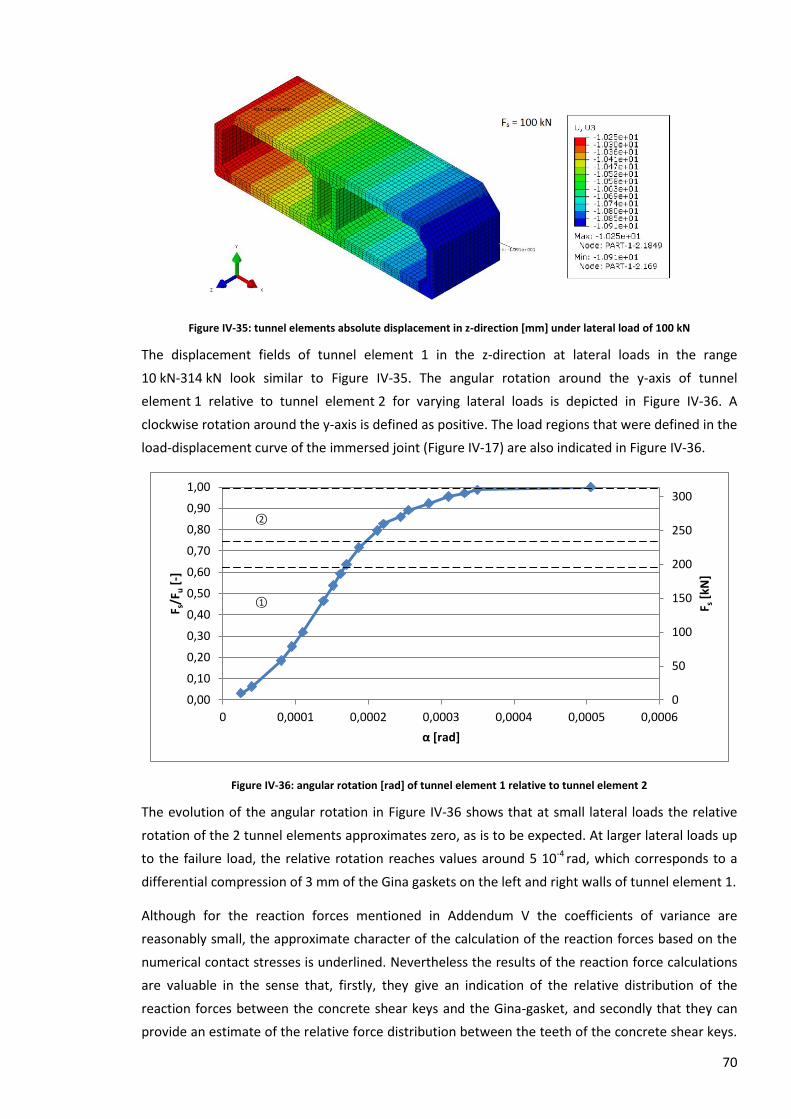
70

Figure IV-35: tunnel elements absolute displacement in z-direction [mm] under lateral load of 100 kN

The displacement fields of tunnel element 1 in the z-direction at lateral loads in the range

10 kN-314 kN look similar to Figure IV-35. The angular rotation around the y-axis of tunnel

element 1 relative to tunnel element 2 for varying lateral loads is depicted in Figure IV-36. A

clockwise rotation around the y-axis is defined as positive. The load regions that were defined in the

load-displacement curve of the immersed joint (Figure IV-17) are also indicated in Figure IV-36.

Figure IV-36: angular rotation [rad] of tunnel element 1 relative to tunnel element 2

The evolution of the angular rotation in Figure IV-36 shows that at small lateral loads the relative

rotation of the 2 tunnel elements approximates zero, as is to be expected. At larger lateral loads up

to the failure load, the relative rotation reaches values around 5 10-4 rad, which corresponds to a

differential compression of 3 mm of the Gina gaskets on the left and right walls of tunnel element 1.

Although for the reaction forces mentioned in Addendum V the coefficients of variance are

reasonably small, the approximate character of the calculation of the reaction forces based on the

numerical contact stresses is underlined. Nevertheless the results of the reaction force calculations

are valuable in the sense that, firstly, they give an indication of the relative distribution of the

reaction forces between the concrete shear keys and the Gina-gasket, and secondly that they can

provide an estimate of the relative force distribution between the teeth of the concrete shear keys.

0

50

100

150

200

250

300

0,00

0,10

0,20

0,30

0,40

0,50

0,60

0,70

0,80

0,90

1,00

0 0,0001 0,0002 0,0003 0,0004 0,0005 0,0006 F s

[kN

]

F s/F

u [

-]

α [rad]

○1

○2

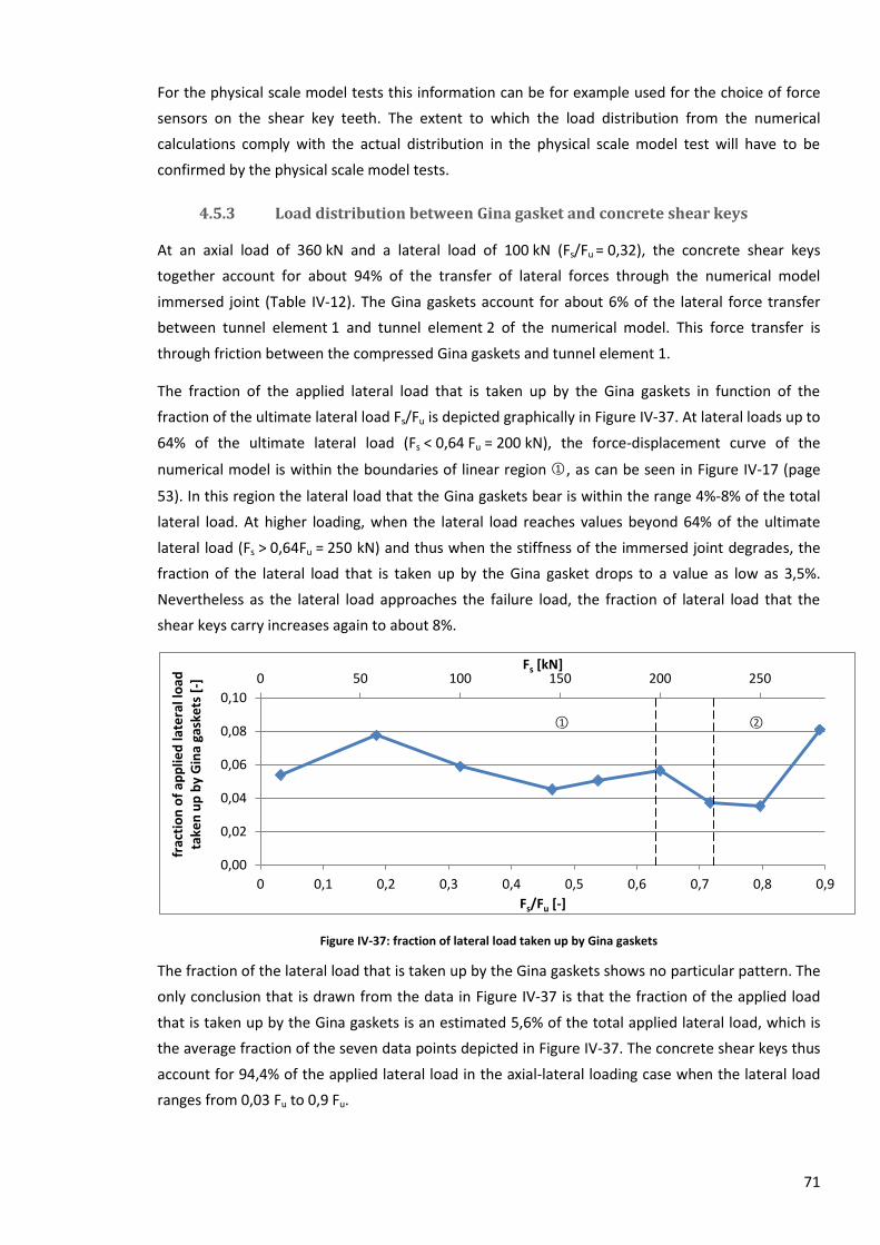
71

For the physical scale model tests this information can be for example used for the choice of force

sensors on the shear key teeth. The extent to which the load distribution from the numerical

calculations comply with the actual distribution in the physical scale model test will have to be

confirmed by the physical scale model tests.

4.5.3 Load distribution between Gina gasket and concrete shear keys

At an axial load of 360 kN and a lateral load of 100 kN (Fs/Fu = 0,32), the concrete shear keys

together account for about 94% of the transfer of lateral forces through the numerical model

immersed joint (Table IV-12). The Gina gaskets account for about 6% of the lateral force transfer

between tunnel element 1 and tunnel element 2 of the numerical model. This force transfer is

through friction between the compressed Gina gaskets and tunnel element 1.

The fraction of the applied lateral load that is taken up by the Gina gaskets in function of the

fraction of the ultimate lateral load Fs/Fu is depicted graphically in Figure IV-37. At lateral loads up to

64% of the ultimate lateral load (Fs < 0,64 Fu = 200 kN), the force-displacement curve of the

numerical model is within the boundaries of linear region ○1 , as can be seen in Figure IV-17 (page

53). In this region the lateral load that the Gina gaskets bear is within the range 4%-8% of the total

lateral load. At higher loading, when the lateral load reaches values beyond 64% of the ultimate

lateral load (Fs > 0,64Fu = 250 kN) and thus when the stiffness of the immersed joint degrades, the

fraction of the lateral load that is taken up by the Gina gasket drops to a value as low as 3,5%.

Nevertheless as the lateral load approaches the failure load, the fraction of lateral load that the

shear keys carry increases again to about 8%.

Figure IV-37: fraction of lateral load taken up by Gina gaskets

The fraction of the lateral load that is taken up by the Gina gaskets shows no particular pattern. The

only conclusion that is drawn from the data in Figure IV-37 is that the fraction of the applied load

that is taken up by the Gina gaskets is an estimated 5,6% of the total applied lateral load, which is

the average fraction of the seven data points depicted in Figure IV-37. The concrete shear keys thus

account for 94,4% of the applied lateral load in the axial-lateral loading case when the lateral load

ranges from 0,03 Fu to 0,9 Fu.

0 50 100 150 200 250

0,00

0,02

0,04

0,06

0,08

0,10

0 0,1 0,2 0,3 0,4 0,5 0,6 0,7 0,8 0,9

Fs [kN]

frac

tio

n o

f ap

plie

d la

tera

l lo

ad

take

n u

p b

y G

ina

gask

ets

[-]

Fs/Fu [-]

○1

○2

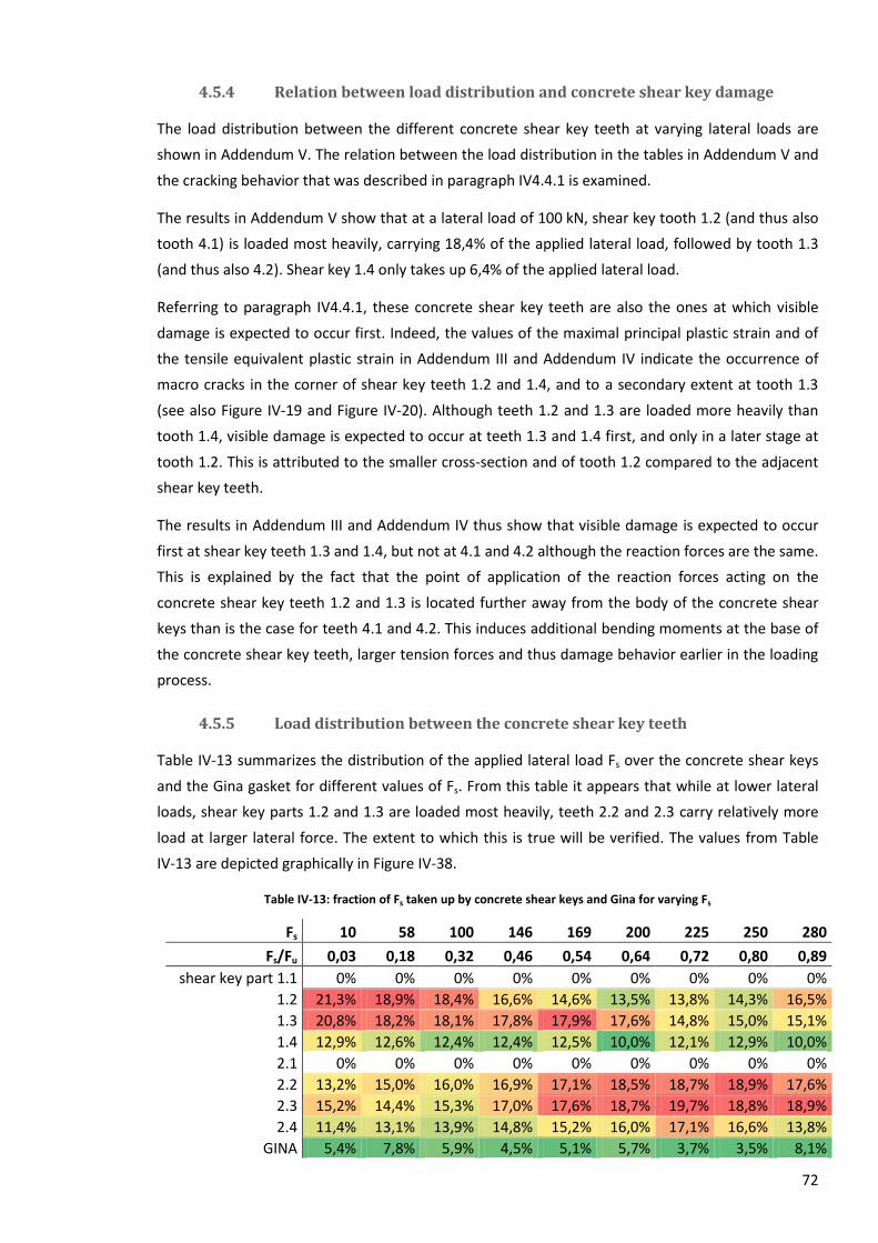
72

4.5.4 Relation between load distribution and concrete shear key damage

The load distribution between the different concrete shear key teeth at varying lateral loads are

shown in Addendum V. The relation between the load distribution in the tables in Addendum V and

the cracking behavior that was described in paragraph IV4.4.1 is examined.

The results in Addendum V show that at a lateral load of 100 kN, shear key tooth 1.2 (and thus also

tooth 4.1) is loaded most heavily, carrying 18,4% of the applied lateral load, followed by tooth 1.3

(and thus also 4.2). Shear key 1.4 only takes up 6,4% of the applied lateral load.

Referring to paragraph IV4.4.1, these concrete shear key teeth are also the ones at which visible

damage is expected to occur first. Indeed, the values of the maximal principal plastic strain and of

the tensile equivalent plastic strain in Addendum III and Addendum IV indicate the occurrence of

macro cracks in the corner of shear key teeth 1.2 and 1.4, and to a secondary extent at tooth 1.3

(see also Figure IV-19 and Figure IV-20). Although teeth 1.2 and 1.3 are loaded more heavily than

tooth 1.4, visible damage is expected to occur at teeth 1.3 and 1.4 first, and only in a later stage at

tooth 1.2. This is attributed to the smaller cross-section and of tooth 1.2 compared to the adjacent

shear key teeth.

The results in Addendum III and Addendum IV thus show that visible damage is expected to occur

first at shear key teeth 1.3 and 1.4, but not at 4.1 and 4.2 although the reaction forces are the same.

This is explained by the fact that the point of application of the reaction forces acting on the

concrete shear key teeth 1.2 and 1.3 is located further away from the body of the concrete shear

keys than is the case for teeth 4.1 and 4.2. This induces additional bending moments at the base of

the concrete shear key teeth, larger tension forces and thus damage behavior earlier in the loading

process.

4.5.5 Load distribution between the concrete shear key teeth

Table IV-13 summarizes the distribution of the applied lateral load Fs over the concrete shear keys

and the Gina gasket for different values of Fs. From this table it appears that while at lower lateral

loads, shear key parts 1.2 and 1.3 are loaded most heavily, teeth 2.2 and 2.3 carry relatively more

load at larger lateral force. The extent to which this is true will be verified. The values from Table

IV-13 are depicted graphically in Figure IV-38.

Table IV-13: fraction of Fs taken up by concrete shear keys and Gina for varying Fs

Fs 10 58 100 146 169 200 225 250 280

Fs/Fu 0,03 0,18 0,32 0,46 0,54 0,64 0,72 0,80 0,89

shear key part 1.1 0% 0% 0% 0% 0% 0% 0% 0% 0%

1.2 21,3% 18,9% 18,4% 16,6% 14,6% 13,5% 13,8% 14,3% 16,5%

1.3 20,8% 18,2% 18,1% 17,8% 17,9% 17,6% 14,8% 15,0% 15,1%

1.4 12,9% 12,6% 12,4% 12,4% 12,5% 10,0% 12,1% 12,9% 10,0%

2.1 0% 0% 0% 0% 0% 0% 0% 0% 0%

2.2 13,2% 15,0% 16,0% 16,9% 17,1% 18,5% 18,7% 18,9% 17,6%

2.3 15,2% 14,4% 15,3% 17,0% 17,6% 18,7% 19,7% 18,8% 18,9%

2.4 11,4% 13,1% 13,9% 14,8% 15,2% 16,0% 17,1% 16,6% 13,8%

GINA 5,4% 7,8% 5,9% 4,5% 5,1% 5,7% 3,7% 3,5% 8,1%

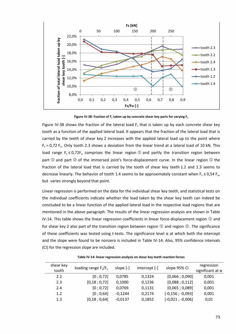
73

Figure IV-38: fraction of Fs taken up by concrete shear key parts for varying Fs

Figure IV-38 shows the fraction of the lateral load Fs that is taken up by each concrete shear key

tooth as a function of the applied lateral load. It appears that the fraction of the lateral load that is

carried by the teeth of shear key 2 increases with the applied lateral load up to the point where

Fs = 0,72 Fu. Only tooth 2.3 shows a deviation from the linear trend at a lateral load of 10 kN. This

load range Fs ≤ 0,72Fu comprises the linear region ○1 and partly the transition region between

part ○1 and part ○2 of the immersed joint's force-displacement curve. In the linear region ○1 the

fraction of the lateral load that is carried by the tooth of shear key teeth 1.2 and 1.3 seems to

decrease linearly. The behavior of tooth 1.4 seems to be approximately constant when Fs ≤ 0,54 Fu,

but varies strongly beyond that point.

Linear regression is performed on the data for the individual shear key teeth, and statistical tests on

the individual coefficients indicate whether the load taken by the shear key teeth can indeed be

concluded to be a linear function of the applied lateral load in the respective load regions that are

mentioned in the above paragraph. The results of the linear regression analysis are shown in Table

IV-14. This table shows the linear regression coefficients in linear force-displacement region ○1 and

for shear key 2 also part of the transition region between region ○1 and region ○2 . The significance

of these coefficients was tested using t-tests. The significance level α at which both the intercept

and the slope were found to be nonzero is included in Table IV-14. Also, 95% confidence intervals

(CI) for the regression slope are included.

Table IV-14: linear regression analysis on shear key teeth reaction forces

shear key tooth

loading range Fs/Fu slope [-] intercept [-] slope 95% CI regression

significant at α

2.2 [0 ; 0,72] 0,0785 0,1324 [0,066 ; 0,090] 0,001

2.3 [0,18 ; 0,72] 0,1000 0,1236 [0,088 ; 0,112] 0,001

2.4 [0 ; 0,72] 0,0769 0,1131 [0,065 ; 0,089] 0,001

1.2 [0 ; 0,64] -0,1244 0,2174 [-0,156 ; -0,093] 0,001

1.3 [0,18 ; 0,64] -0,0137 0,1852 [-0,021 ; -0,006] 0,01

0 50 100 150 200 250

8,0%

10,0%

12,0%

14,0%

16,0%

18,0%

20,0%

22,0%

0,0 0,1 0,2 0,3 0,4 0,5 0,6 0,7 0,8 0,9

Fs [kN]

frac

tio

n o

f to

tal l

ate

ral l

oad

tak

en

up

by

she

ar k

ey

too

th [

-]

Fs/Fu [-]

tooth 2.3

tooth 2.2

tooth 2.4

tooth 1.3

tooth 1.2

tooth 1.4

○1 ○2

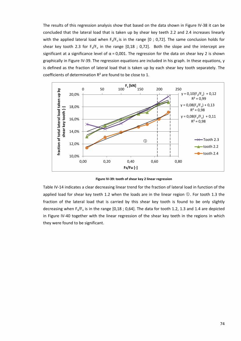
74

The results of this regression analysis show that based on the data shown in Figure IV-38 it can be

concluded that the lateral load that is taken up by shear key teeth 2.2 and 2.4 increases linearly

with the applied lateral load when Fs/Fu is in the range [0 ; 0,72]. The same conclusion holds for

shear key tooth 2.3 for Fs/Fu in the range [0,18 ; 0,72]. Both the slope and the intercept are

significant at a significance level of α = 0,001. The regression for the data on shear key 2 is shown

graphically in Figure IV-39. The regression equations are included in his graph. In these equations, y

is defined as the fraction of lateral load that is taken up by each shear key tooth separately. The

coefficients of determination R² are found to be close to 1.

Figure IV-39: tooth of shear key 2 linear regression

Table IV-14 indicates a clear decreasing linear trend for the fraction of lateral load in function of the

applied load for shear key teeth 1.2 when the loads are in the linear region ○1 . For tooth 1.3 the

fraction of the lateral load that is carried by this shear key tooth is found to be only slightly

decreasing when Fs/Fu is in the range [0,18 ; 0,64]. The data for tooth 1.2, 1.3 and 1.4 are depicted

in Figure IV-40 together with the linear regression of the shear key teeth in the regions in which

they were found to be significant.

y = 0,10(Fs/Fu) + 0,12 R² = 0,99

y = 0,08(Fs/Fu) + 0,13 R² = 0,98

y = 0,08(Fs/Fu) + 0,11 R² = 0,98

0 50 100 150 200 250

10,0%

12,0%

14,0%

16,0%

18,0%

20,0%

0,00 0,20 0,40 0,60 0,80

Fs [kN]

frac

tio

n o

f to

tal l

ate

ral l

oad

tak

en

up

by

she

ar k

ey

too

th [

-]

Fs/Fu [-]

Tooth 2.3

tooth 2.2

tooth 2.4

○1

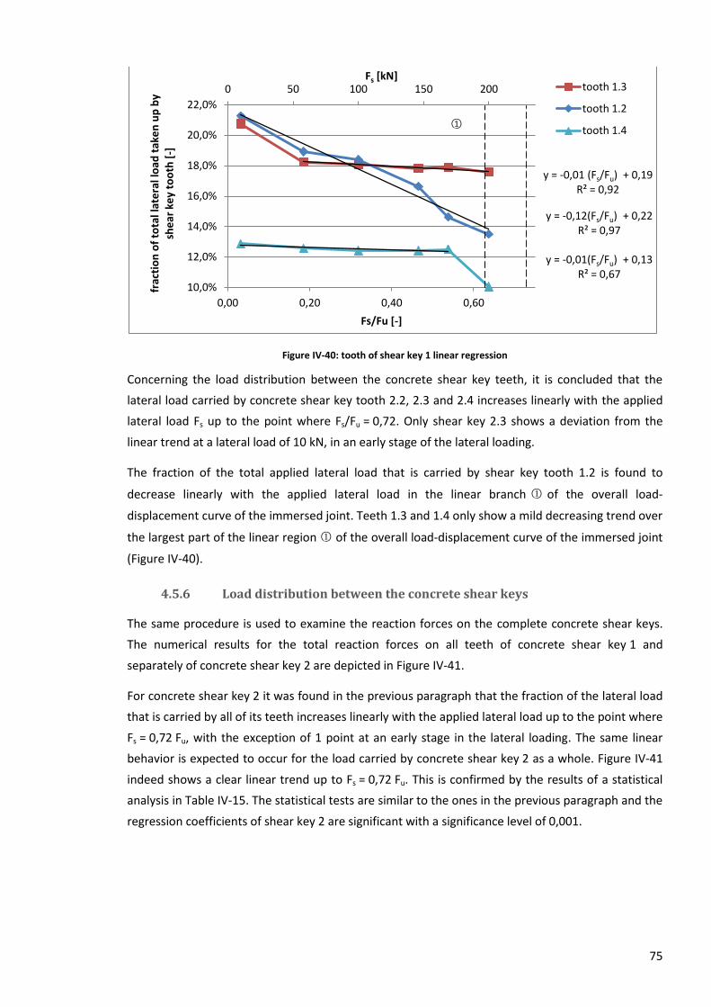
75

Figure IV-40: tooth of shear key 1 linear regression

Concerning the load distribution between the concrete shear key teeth, it is concluded that the

lateral load carried by concrete shear key tooth 2.2, 2.3 and 2.4 increases linearly with the applied

lateral load Fs up to the point where Fs/Fu = 0,72. Only shear key 2.3 shows a deviation from the

linear trend at a lateral load of 10 kN, in an early stage of the lateral loading.

The fraction of the total applied lateral load that is carried by shear key tooth 1.2 is found to

decrease linearly with the applied lateral load in the linear branch ○1 of the overall load-

displacement curve of the immersed joint. Teeth 1.3 and 1.4 only show a mild decreasing trend over

the largest part of the linear region ○1 of the overall load-displacement curve of the immersed joint

(Figure IV-40).

4.5.6 Load distribution between the concrete shear keys

The same procedure is used to examine the reaction forces on the complete concrete shear keys.

The numerical results for the total reaction forces on all teeth of concrete shear key 1 and

separately of concrete shear key 2 are depicted in Figure IV-41.

For concrete shear key 2 it was found in the previous paragraph that the fraction of the lateral load

that is carried by all of its teeth increases linearly with the applied lateral load up to the point where

Fs = 0,72 Fu, with the exception of 1 point at an early stage in the lateral loading. The same linear

behavior is expected to occur for the load carried by concrete shear key 2 as a whole. Figure IV-41

indeed shows a clear linear trend up to Fs = 0,72 Fu. This is confirmed by the results of a statistical

analysis in Table IV-15. The statistical tests are similar to the ones in the previous paragraph and the

regression coefficients of shear key 2 are significant with a significance level of 0,001.

y = -0,01 (Fs/Fu) + 0,19 R² = 0,92

y = -0,12(Fs/Fu) + 0,22 R² = 0,97

y = -0,01(Fs/Fu) + 0,13 R² = 0,67

0 50 100 150 200

10,0%

12,0%

14,0%

16,0%

18,0%

20,0%

22,0%

0,00 0,20 0,40 0,60

Fs [kN]

frac

tio

n o

f to

tal l

ate

ral l

oad

tak

en

up

by

she

ar k

ey

too

th [

-]

Fs/Fu [-]

tooth 1.3

tooth 1.2

tooth 1.4 ○1

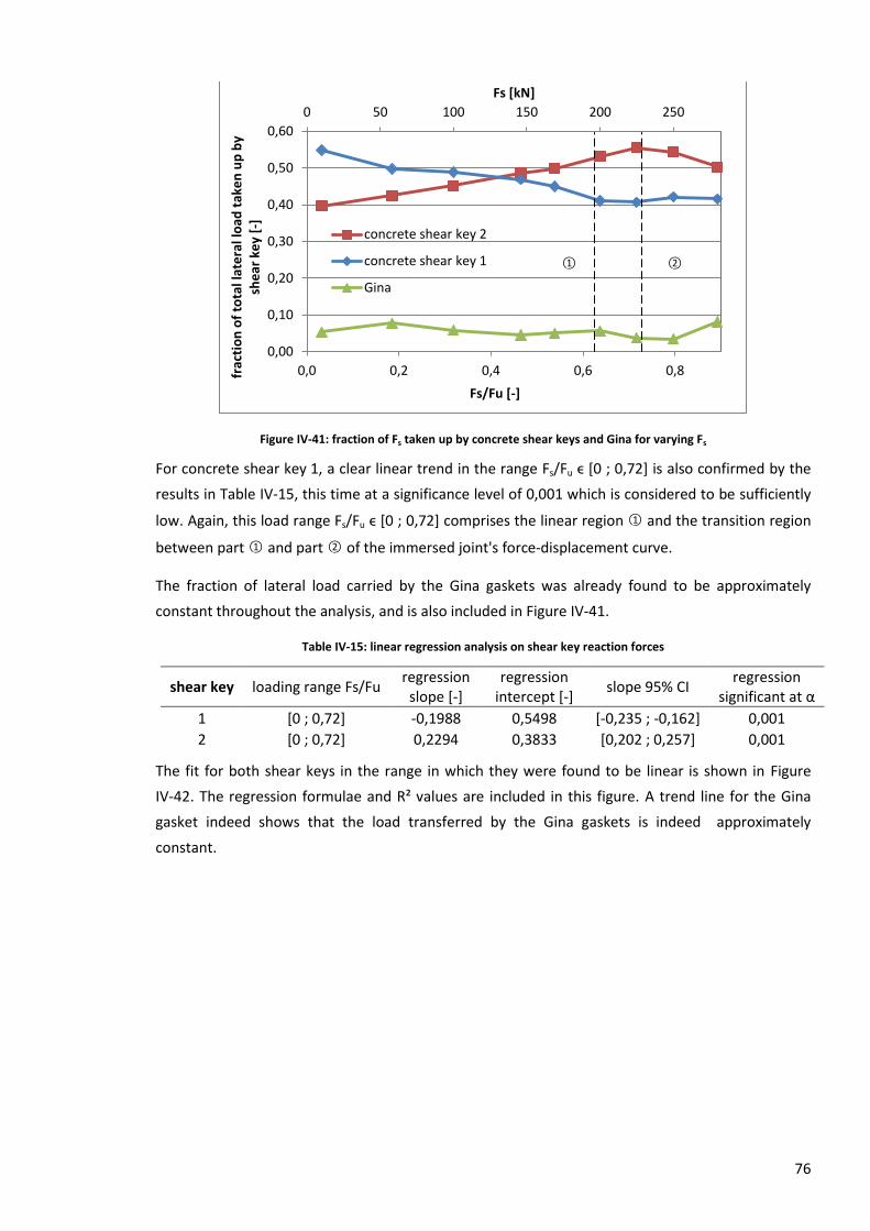
76

Figure IV-41: fraction of Fs taken up by concrete shear keys and Gina for varying Fs

For concrete shear key 1, a clear linear trend in the range Fs/Fu ϵ [0 ; 0,72] is also confirmed by the

results in Table IV-15, this time at a significance level of 0,001 which is considered to be sufficiently

low. Again, this load range Fs/Fu ϵ [0 ; 0,72] comprises the linear region ○1 and the transition region

between part ○1 and part ○2 of the immersed joint's force-displacement curve.

The fraction of lateral load carried by the Gina gaskets was already found to be approximately

constant throughout the analysis, and is also included in Figure IV-41.

Table IV-15: linear regression analysis on shear key reaction forces

shear key loading range Fs/Fu regression

slope [-] regression

intercept [-] slope 95% CI

regression significant at α

1 [0 ; 0,72] -0,1988 0,5498 [-0,235 ; -0,162] 0,001

2 [0 ; 0,72] 0,2294 0,3833 [0,202 ; 0,257] 0,001

The fit for both shear keys in the range in which they were found to be linear is shown in Figure

IV-42. The regression formulae and R² values are included in this figure. A trend line for the Gina

gasket indeed shows that the load transferred by the Gina gaskets is indeed approximately

constant.

0 50 100 150 200 250

0,00

0,10

0,20

0,30

0,40

0,50

0,60

0,0 0,2 0,4 0,6 0,8

Fs [kN]

frac

tio

n o

f to

tal l

ate

ral l

oad

tak

en

up

by

she

ar k

ey

[-]

Fs/Fu [-]

concrete shear key 2


Gina

○1 ○2

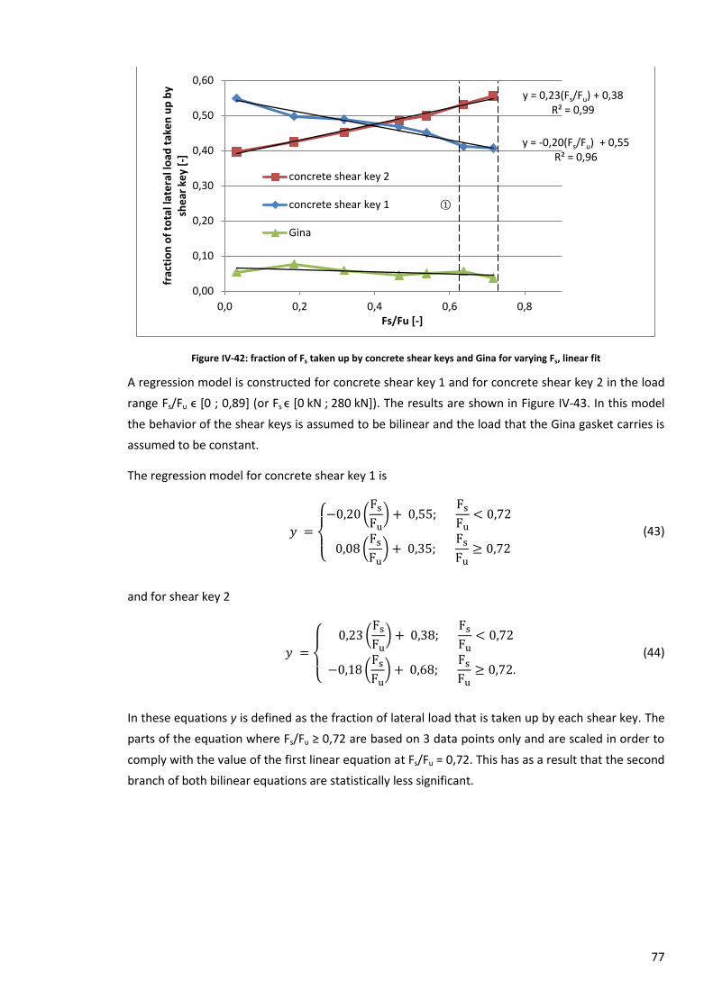
77

Figure IV-42: fraction of Fs taken up by concrete shear keys and Gina for varying Fs, linear fit

A regression model is constructed for concrete shear key 1 and for concrete shear key 2 in the load

range Fs/Fu ϵ [0 ; 0,89] (or Fs ϵ [0 kN ; 280 kN]). The results are shown in Figure IV-43. In this model

the behavior of the shear keys is assumed to be bilinear and the load that the Gina gasket carries is

assumed to be constant.

The regression model for concrete shear key 1 is

(43)

and for shear key 2

(44)

In these equations y is defined as the fraction of lateral load that is taken up by each shear key. The

parts of the equation where Fs/Fu ≥ 0,72 are based on 3 data points only and are scaled in order to

comply with the value of the first linear equation at Fs/Fu = 0,72. This has as a result that the second

branch of both bilinear equations are statistically less significant.

y = 0,23(Fs/Fu) + 0,38 R² = 0,99

y = -0,20(Fs/Fu) + 0,55 R² = 0,96

0,00

0,10

0,20

0,30

0,40

0,50

0,60

0,0 0,2 0,4 0,6 0,8

frac

tio

n o

f to

tal l

ate

ral l

oad

tak

en

up

by

she

ar k

ey

[-]

Fs/Fu [-]



Gina

○1

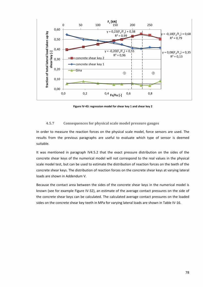
78

Figure IV-43: regression model for shear key 1 and shear key 2

4.5.7 Consequences for physical scale model pressure gauges

In order to measure the reaction forces on the physical scale model, force sensors are used. The

results from the previous paragraphs are useful to evaluate which type of sensor is deemed

suitable.

It was mentioned in paragraph IV4.5.2 that the exact pressure distribution on the sides of the

concrete shear keys of the numerical model will not correspond to the real values in the physical

scale model test, but can be used to estimate the distribution of reaction forces on the teeth of the

concrete shear keys. The distribution of reaction forces on the concrete shear keys at varying lateral

loads are shown in Addendum V.

Because the contact area between the sides of the concrete shear keys in the numerical model is

known (see for example Figure IV-32), an estimate of the average contact pressures on the side of

the concrete shear keys can be calculated. The calculated average contact pressures on the loaded

sides on the concrete shear key teeth in MPa for varying lateral loads are shown in Table IV-16.

y = 0,23(Fs/Fu) + 0,38 R² = 0,99

y = -0,20(Fs/Fu) + 0,55 R² = 0,96

y = -0,18(Fs/Fu) + 0,68 R² = 0,79

y = 0,08(Fs/Fu) + 0,35 R² = 0,13

0 50 100 150 200 250

0,00

0,10

0,20

0,30

0,40

0,50

0,60

0,0 0,2 0,4 0,6 0,8

Fs [kN]

frac

tio

n o

f to

tal l

ate

ral l

oad

tak

en

up

by

she

ar k

ey

[-]

Fs/Fu [-]



Gina ○1 ○2

79

Table IV-16: calculated average contact pressures on concrete shear key teeth [N/mm²]

Fs [kN]: 100 146 169 200 225 250 280

shear key part 1.1 0 0 0 0 0 0 0

1.2 1,60 2,11 2,15 2,35 2,70 3,10 4,01

1.3 1,57 2,26 2,63 3,06 2,90 3,26 3,68

1.4 1,08 1,58 1,84 1,75 2,36 2,80 2,43

2.1 0 0 0 0 0 0 0

2.2 1,39 2,14 2,52 3,22 3,67 4,12 4,28

2.3 1,33 2,16 2,59 3,25 3,85 4,09 4,60

2.4 1,21 1,87 2,23 2,79 3,35 3,60 3,37

The force sensors will be placed between the concrete shear keys and the rubber supports (Figure

IV-31), and thus have to be sufficiently thin. Additionally the sensors have to be able to measure the

loads accurately at all loading stages.

As Figure IV-33 and Figure IV-34 show, the contact pressures are not uniform over the side area of

the concrete shear keys. This means that the average values in Table IV-16 are not conservative

enough to make a decision on which force sensors can be used. Instead of a uniform distribution, a

triangular stress distribution over the contact area between the concrete shear keys is assumed. A

theoretical triangular stress distribution on the teeth of concrete shear key 2 is shown in Figure

IV-44. This stress distribution is in accordance with the numerical results for the contact stresses for

shear key 2, shown in Figure IV-34. Nevertheless it is underlined that the triangular load distribution

is an extreme situation that is used to estimate the maximum pressure that could occur locally.

Figure IV-44: theoretical triangular load distribution on shear key 2

The use of a triangular distribution is justified by the fact that at the contact surface between two

concrete shear key teeth, the contact pressure can become zero, but cannot become negative (no

tension forces can be transmitted). Although the exact pressure distribution that will occur in the

physical scale model test is unknown, assuming zero pressure at one point on each contact surface

is assumed to be a fairly conservative approach. This corresponds to the point where the concrete

shear key teeth just start to detach at one point. The numerical results also indicate that the contact

area between the concrete shear key teeth does not diminish during the loading steps, so that

besides the variation of stresses, a reduction in contact area is not taken into account in the

estimation of the maximum contact stress.

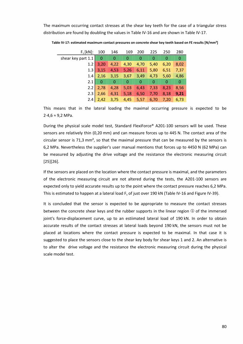
80

The maximum occurring contact stresses at the shear key teeth for the case of a triangular stress

distribution are found by doubling the values in Table IV-16 and are shown in Table IV-17.

Table IV-17: estimated maximum contact pressures on concrete shear key teeth based on FE results [N/mm²]

Fs [kN]: 100 146 169 200 225 250 280

shear key part 1.1 0 0 0 0 0 0 0

1.2 3,20 4,22 4,30 4,70 5,40 6,20 8,02

1.3 3,15 4,53 5,26 6,11 5,80 6,51 7,37

1.4 2,16 3,15 3,67 3,49 4,73 5,60 4,86

2.1 0 0 0 0 0 0 0

2.2 2,78 4,28 5,03 6,43 7,33 8,23 8,56

2.3 2,66 4,31 5,18 6,50 7,70 8,18 9,21

2.4 2,42 3,75 4,45 5,57 6,70 7,20 6,73

This means that in the lateral loading the maximal occurring pressure is expected to be

2 4,6 ≈ 9,2 MPa.

During the physical scale model test, Standard FlexiForce® A201-100 sensors will be used. These

sensors are relatively thin (0,20 mm) and can measure forces up to 445 N. The contact area of the

circular sensor is 71,3 mm², so that the maximal pressure that can be measured by the sensors is

6,2 MPa. Nevertheless the supplier's user manual mentions that forces up to 4450 N (62 MPa) can

be measured by adjusting the drive voltage and the resistance the electronic measuring circuit

[25][26].

If the sensors are placed on the location where the contact pressure is maximal, and the parameters

of the electronic measuring circuit are not altered during the tests, the A201-100 sensors are

expected only to yield accurate results up to the point where the contact pressure reaches 6,2 MPa.

This is estimated to happen at a lateral load Fs of just over 190 kN (Table IV-16 and Figure IV-39).

It is concluded that the sensor is expected to be appropriate to measure the contact stresses

between the concrete shear keys and the rubber supports in the linear region ○1 of the immersed

joint's force-displacement curve, up to an estiimated lateral load of 190 kN. In order to obtain

accurate results of the contact stresses at lateral loads beyond 190 kN, the sensors must not be

placed at locations where the contact pressure is expected to be maximal. In that case it is

suggested to place the sensors close to the shear key body for shear keys 1 and 2. An alternative is

to alter the drive voltage and the resistance the electronic measuring circuit during the physical

scale model test.

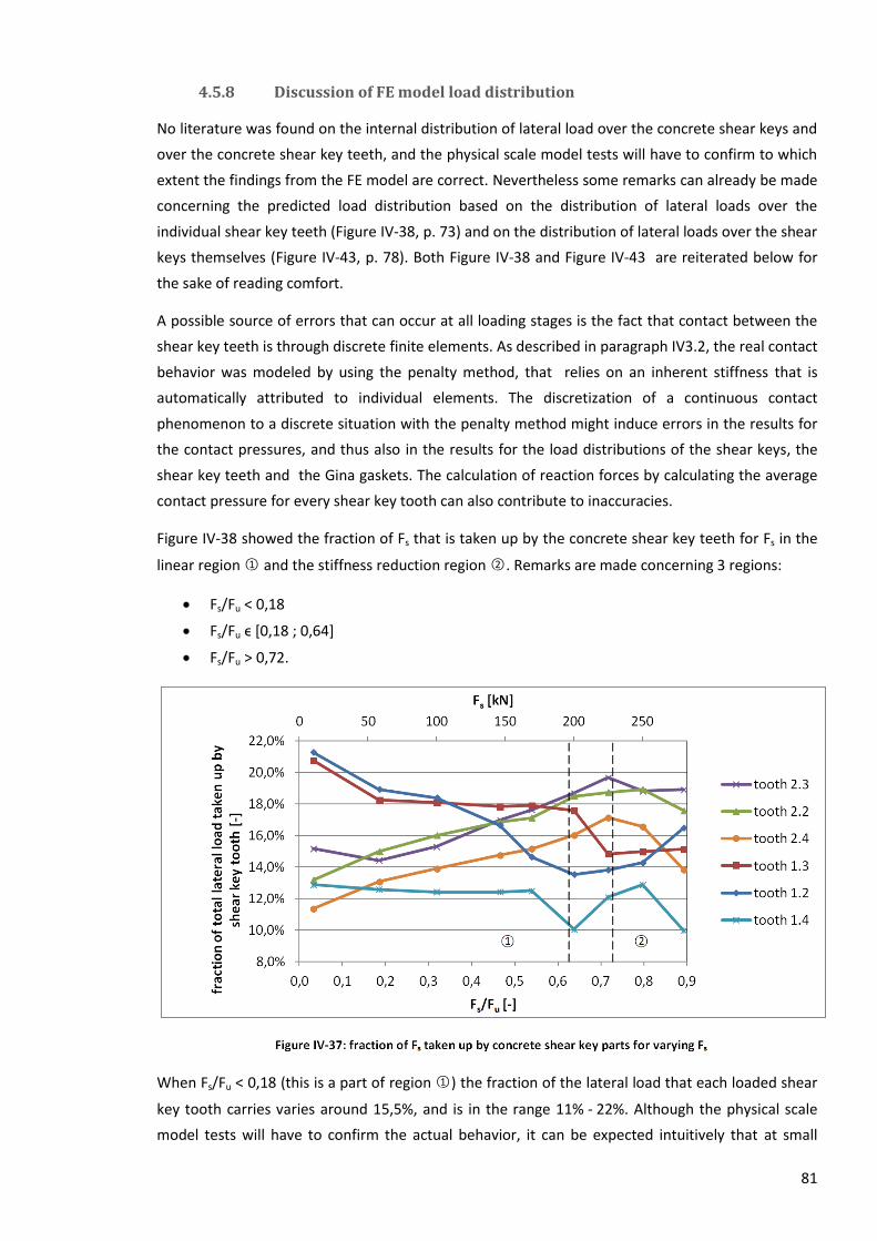
81

4.5.8 Discussion of FE model load distribution

No literature was found on the internal distribution of lateral load over the concrete shear keys and

over the concrete shear key teeth, and the physical scale model tests will have to confirm to which

extent the findings from the FE model are correct. Nevertheless some remarks can already be made

concerning the predicted load distribution based on the distribution of lateral loads over the

individual shear key teeth (Figure IV-38, p. 73) and on the distribution of lateral loads over the shear

keys themselves (Figure IV-43, p. 78). Both Figure IV-38 and Figure IV-43 are reiterated below for

the sake of reading comfort.

A possible source of errors that can occur at all loading stages is the fact that contact between the

shear key teeth is through discrete finite elements. As described in paragraph IV3.2, the real contact

behavior was modeled by using the penalty method, that relies on an inherent stiffness that is

automatically attributed to individual elements. The discretization of a continuous contact

phenomenon to a discrete situation with the penalty method might induce errors in the results for

the contact pressures, and thus also in the results for the load distributions of the shear keys, the

shear key teeth and the Gina gaskets. The calculation of reaction forces by calculating the average

contact pressure for every shear key tooth can also contribute to inaccuracies.

Figure IV-38 showed the fraction of Fs that is taken up by the concrete shear key teeth for Fs in the

linear region ○1 and the stiffness reduction region ○2 . Remarks are made concerning 3 regions:

Fs/Fu < 0,18

Fs/Fu ϵ [0,18 ; 0,64]

Fs/Fu > 0,72.

When Fs/Fu < 0,18 (this is a part of region ○1 ) the fraction of the lateral load that each loaded shear

key tooth carries varies around 15,5%, and is in the range 11% - 22%. Although the physical scale

model tests will have to confirm the actual behavior, it can be expected intuitively that at small

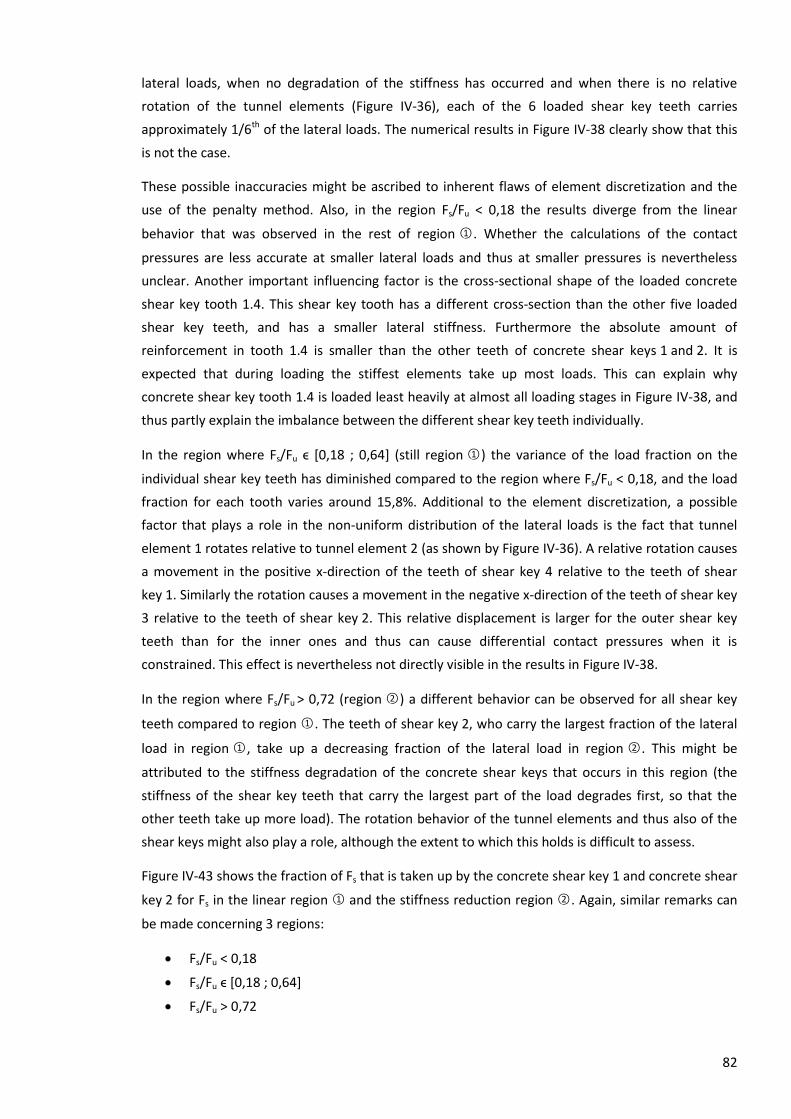
82

lateral loads, when no degradation of the stiffness has occurred and when there is no relative

rotation of the tunnel elements (Figure IV-36), each of the 6 loaded shear key teeth carries

approximately 1/6th of the lateral loads. The numerical results in Figure IV-38 clearly show that this

is not the case.

These possible inaccuracies might be ascribed to inherent flaws of element discretization and the

use of the penalty method. Also, in the region Fs/Fu < 0,18 the results diverge from the linear

behavior that was observed in the rest of region ○1 . Whether the calculations of the contact

pressures are less accurate at smaller lateral loads and thus at smaller pressures is nevertheless

unclear. Another important influencing factor is the cross-sectional shape of the loaded concrete

shear key tooth 1.4. This shear key tooth has a different cross-section than the other five loaded

shear key teeth, and has a smaller lateral stiffness. Furthermore the absolute amount of

reinforcement in tooth 1.4 is smaller than the other teeth of concrete shear keys 1 and 2. It is

expected that during loading the stiffest elements take up most loads. This can explain why

concrete shear key tooth 1.4 is loaded least heavily at almost all loading stages in Figure IV-38, and

thus partly explain the imbalance between the different shear key teeth individually.

In the region where Fs/Fu ϵ [0,18 ; 0,64] (still region ○1 ) the variance of the load fraction on the

individual shear key teeth has diminished compared to the region where Fs/Fu < 0,18, and the load

fraction for each tooth varies around 15,8%. Additional to the element discretization, a possible

factor that plays a role in the non-uniform distribution of the lateral loads is the fact that tunnel

element 1 rotates relative to tunnel element 2 (as shown by Figure IV-36). A relative rotation causes

a movement in the positive x-direction of the teeth of shear key 4 relative to the teeth of shear

key 1. Similarly the rotation causes a movement in the negative x-direction of the teeth of shear key

3 relative to the teeth of shear key 2. This relative displacement is larger for the outer shear key

teeth than for the inner ones and thus can cause differential contact pressures when it is

constrained. This effect is nevertheless not directly visible in the results in Figure IV-38.

In the region where Fs/Fu > 0,72 (region ○2 ) a different behavior can be observed for all shear key

teeth compared to region ○1 . The teeth of shear key 2, who carry the largest fraction of the lateral

load in region ○1 , take up a decreasing fraction of the lateral load in region ○2 . This might be

attributed to the stiffness degradation of the concrete shear keys that occurs in this region (the

stiffness of the shear key teeth that carry the largest part of the load degrades first, so that the

other teeth take up more load). The rotation behavior of the tunnel elements and thus also of the

shear keys might also play a role, although the extent to which this holds is difficult to assess.

Figure IV-43 shows the fraction of Fs that is taken up by the concrete shear key 1 and concrete shear

key 2 for Fs in the linear region ○1 and the stiffness reduction region ○2 . Again, similar remarks can

be made concerning 3 regions:

Fs/Fu < 0,18

Fs/Fu ϵ [0,18 ; 0,64]

Fs/Fu > 0,72

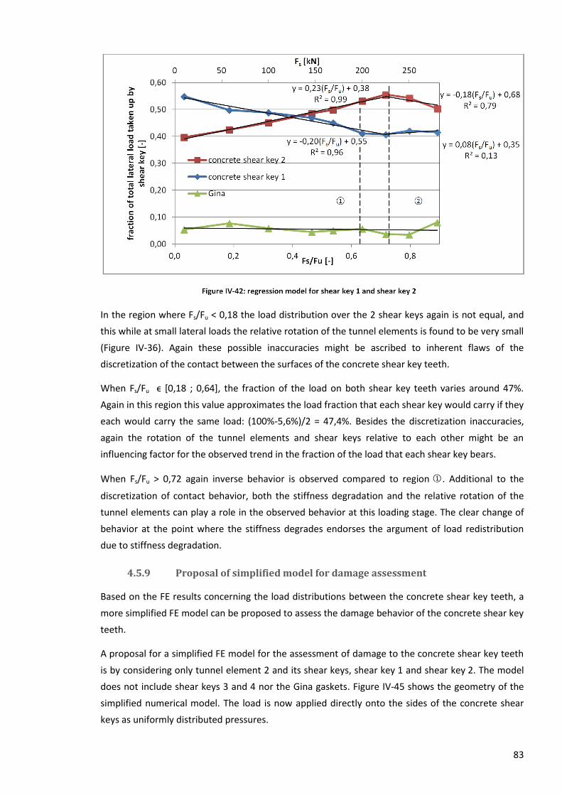
83

In the region where Fs/Fu < 0,18 the load distribution over the 2 shear keys again is not equal, and

this while at small lateral loads the relative rotation of the tunnel elements is found to be very small

(Figure IV-36). Again these possible inaccuracies might be ascribed to inherent flaws of the

discretization of the contact between the surfaces of the concrete shear key teeth.

When Fs/Fu ϵ [0,18 ; 0,64], the fraction of the load on both shear key teeth varies around 47%.

Again in this region this value approximates the load fraction that each shear key would carry if they

each would carry the same load: (100%-5,6%)/2 = 47,4%. Besides the discretization inaccuracies,

again the rotation of the tunnel elements and shear keys relative to each other might be an

influencing factor for the observed trend in the fraction of the load that each shear key bears.

When Fs/Fu > 0,72 again inverse behavior is observed compared to region ○1 . Additional to the

discretization of contact behavior, both the stiffness degradation and the relative rotation of the

tunnel elements can play a role in the observed behavior at this loading stage. The clear change of

behavior at the point where the stiffness degrades endorses the argument of load redistribution

due to stiffness degradation.

4.5.9 Proposal of simplified model for damage assessment

Based on the FE results concerning the load distributions between the concrete shear key teeth, a

more simplified FE model can be proposed to assess the damage behavior of the concrete shear key

teeth.

A proposal for a simplified FE model for the assessment of damage to the concrete shear key teeth

is by considering only tunnel element 2 and its shear keys, shear key 1 and shear key 2. The model

does not include shear keys 3 and 4 nor the Gina gaskets. Figure IV-45 shows the geometry of the

simplified numerical model. The load is now applied directly onto the sides of the concrete shear

keys as uniformly distributed pressures.

84

Figure IV-45: simplified numerical model

The Gina gaskets were found earlier to carry an estimated 5,6% of the total lateral load. Figure IV-37

indeed shows that in this load range(Fs/Fu in the range 0,20 to 0,5) the load fraction of the Gina is

approximately equal to this value.

Based on the results for the loads on the individual shear key teeth in Figure IV-38, a possible

loading scheme for the fraction of the lateral load that is applied on each shear key tooth is

depicted in Figure IV-46. This load distribution is expected to yield most conform results for the

damage behavior of the shear key teeth in the load range were 0,20 < Fs/Fu < 0,50 because in this

loading range they correspond best to the values from Figure IV-38. In the Figure IV-46 the fractions

for all the shear key teeth together add up to 94,4%.

Figure IV-46: simplified of lateral loading on concrete shear key teeth (proposal)

The equivalent absolute load and the equivalent relative load at which the alternative FE model

shows that cracking initiates is summarized in Table IV-18. The same criteria for cracking initiation

4%

6%

8%

10%

12%

14%

16%

18%

20%

22%

0,00 0,20 0,40 0,60

frac

tio

n o

f to

tal l

ate

ral l

oad

tak

en

u

p b

y sh

ear

ke

y to

oth

[-]

Fs/Fu [kN]

tooth 1.2 & 1.3

other teeth

tooth 1.4

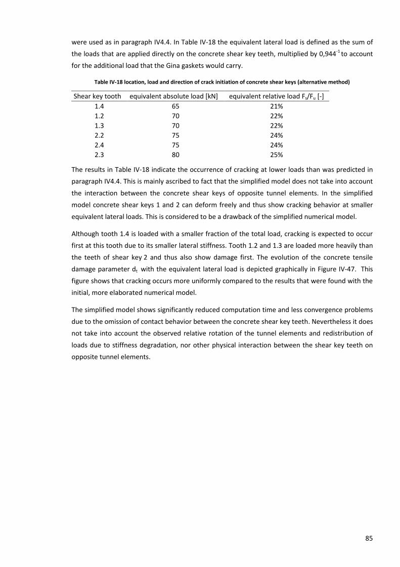
85

were used as in paragraph IV4.4. In Table IV-18 the equivalent lateral load is defined as the sum of

the loads that are applied directly on the concrete shear key teeth, multiplied by 0,944-1 to account

for the additional load that the Gina gaskets would carry.

Table IV-18 location, load and direction of crack initiation of concrete shear keys (alternative method)

Shear key tooth equivalent absolute load [kN] equivalent relative load Fs/Fu [-]

1.4 65 21%

1.2 70 22%

1.3 70 22%

2.2 75 24%

2.4 75 24%

2.3 80 25%

The results in Table IV-18 indicate the occurrence of cracking at lower loads than was predicted in

paragraph IV4.4. This is mainly ascribed to fact that the simplified model does not take into account

the interaction between the concrete shear keys of opposite tunnel elements. In the simplified

model concrete shear keys 1 and 2 can deform freely and thus show cracking behavior at smaller

equivalent lateral loads. This is considered to be a drawback of the simplified numerical model.

Although tooth 1.4 is loaded with a smaller fraction of the total load, cracking is expected to occur

first at this tooth due to its smaller lateral stiffness. Tooth 1.2 and 1.3 are loaded more heavily than

the teeth of shear key 2 and thus also show damage first. The evolution of the concrete tensile

damage parameter dt with the equivalent lateral load is depicted graphically in Figure IV-47. This

figure shows that cracking occurs more uniformly compared to the results that were found with the

initial, more elaborated numerical model.

The simplified model shows significantly reduced computation time and less convergence problems

due to the omission of contact behavior between the concrete shear key teeth. Nevertheless it does

not take into account the observed relative rotation of the tunnel elements and redistribution of

loads due to stiffness degradation, nor other physical interaction between the shear key teeth on

opposite tunnel elements.

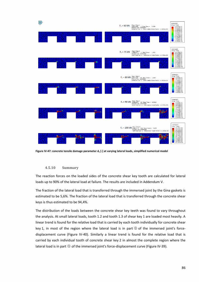
86

Figure IV-47: concrete tensile damage parameter dt [-] at varying lateral loads, simplified numerical model

4.5.10 Summary

The reaction forces on the loaded sides of the concrete shear key tooth are calculated for lateral

loads up to 90% of the lateral load at failure. The results are included in Addendum V.

The fraction of the lateral load that is transferred through the immersed joint by the Gina gaskets is

estimated to be 5,6%. The fraction of the lateral load that is transferred through the concrete shear

keys is thus estimated to be 94,4%.

The distribution of the loads between the concrete shear key teeth was found to vary throughout

the analysis. At small lateral loads, tooth 1.2 and tooth 1.3 of shear key 1 are loaded most heavily. A

linear trend is found for the relative load that is carried by each tooth individually for concrete shear

key 1, in most of the region where the lateral load is in part ○1 of the immersed joint's force-

displacement curve (Figure IV-40). Similarly a linear trend is found for the relative load that is

carried by each individual tooth of concrete shear key 2 in almost the complete region where the

lateral load is in part ○1 of the immersed joint's force-displacement curve (Figure IV-39).

87

For the concrete shear keys as entities, it is found that while at smaller lateral loads reaction forces

are largest at concrete shear key 1, the relative amount of load that concrete shear key 1 carries

decreases linearly with the applied lateral load when it is in the linear region ○1 and when it is in the

transition zone between regions ○1 and ○2 of the load-displacement curve. In region ○2 on the

other hand, the relative amount of load that concrete shear key 1 carries is concluded to increase

linearly with the applied lateral load. For concrete shear key 2 it is found that the opposite holds: a

linear increase up to the point where the lateral load reaches region ○2 of the load-displacement

curve, and a linear decrease beyond this point (Figure IV-43). Bilinear regression equations were

constructed for both shear keys (equations (43) and (44)). Remarks were made concerning the

outcome of the numerical results, especially at small lateral loads, and the physical scale model

tests can be used to verify to which extent the findings from the FE model are correct. Based on the

results for the internal load distribution in the immersed joint, a reduced but strongly simplified FE

model of the immersed joint was proposed with which the damage behavior of the immersed joint

can be assessed to a limited extent.

88

V Conclusions

The main objective of this dissertation was to predict the structural behavior of the concrete shear

keys that will occur in a 1:5 physical scale model of the Nanchang Red Valley immersed tunnel,

using a FE model of an immersed joint.

Several material models for the different constituents of the immersed joint were investigated and

the used material models were elaborated. For plain concrete, the damaged plasticity model

according to Lubliner [15] and Lee [17] was used. Steel reinforcement was defined in the FE model

by using the embedded regions method, for which the steel material behavior was assumed plastic

with isotropic hardening. For the rubber of the Gina gaskets, a Mooney-Rivlin material model was

used. For the modeling of concrete, viscoplastic regularization was necessary to overcome

convergence problems when the stiffness of the concrete has degraded significantly.

Dimensional similitude between the FE model and the tunnel prototype was obtained by using the

scaling parameters Sx= SL=1/5 and SE=1. The reinforcement ratio of the FE model was nevertheless

lowered compared to the tunnel prototype to comply with the design of the physical scale model

test. The (scaled) axial load acting on the FE model's immersed joint was also altered to comply with

the design of the physical scale model test.

The degradation of the stiffness of the immersed joint was investigated. Linear force-displacement

behavior, incremental stiffness degradation and complete loss of stiffness occurred in 3 distinct

regions in the load-displacement curve of the immersed joint.

Cracking behavior was assessed using the damaged plasticity model for concrete. Visible cracking of

the concrete shear keys is expected to occur in the physical scale model at a lateral load of above

25% of the ultimate lateral load. The damage that occurred in the FE model was noticed to be in

accordance with the degradation of the joint stiffness.

The reaction forces on the loaded side of the concrete shear key teeth were calculated for lateral

loads up to 90% of the lateral load at failure. The distribution of the applied lateral load between

the Gina gaskets and the concrete shear keys was studied. The fraction of the applied lateral load

89

that is transferred through the immersed joint by the Gina gaskets was concluded to be 5,6% on

average, with limited fluctuations.

Concerning the fraction of the applied lateral load that is taken up by concrete shear keys 1 and 2,

bilinear models were proposed for both concrete shear keys. On the level of individual shear key

teeth it was found that at lower lateral loads shear key teeth 1.2 and 1.3 are loaded most heavily,

and that this shifts to shear key teeth 2.2 and 2.3 at larger lateral loading. The relation between the

applied lateral load and the fraction of load that is taken up by individual shear key teeth showed to

be linear over large but distinct ranges of the applied lateral load. The load distribution between

and within the concrete shear keys showed to be in accordance with the FE model's damage

behavior and the stiffness degradation of the immersed joint. The load distribution that was

obtained from the numerical model was used to make preliminary predictions for the load sensors

for the physical scale model test on the construction site in Nanchang. Some important remarks

were made concerning the accuracy of the outcome of the numerical results, especially at small

lateral loads. Based on the results for the internal load distribution in the immersed joint, a reduced

but strongly simplified FE model of the immersed joint was proposed with which the damage

behavior of the immersed joint can be assessed to a limited extent.

Some recommendations can be made concerning the calibration of future FE models

Modification of the mesh of the concrete shear keys could further enhance the numerical

results

Contact methods other than the penalty method can be investigated to simulate contact

behavior between the concrete shear keys

Adding the rubber supports between shear key teeth to the model could better represent

the real contact conditions

Modifications to the viscoplastic regularization parameter μ can have an effect on the

accuracy of the FE results

The uniaxial damage parameters dt and dc for concrete can be calculated using different

methods, and can be calibrated further with results from physical tests.

90

VI References

[1] XIAO W., YU, H., YUAN, Y., TAERWE, L., RUI, C. , “Compression-bending behavior of a scaled

immersion joint”, August 2014

[2] BAI Y., "Underground Engineering", September 2015, course syllabus, Tongji University , pp.

114-175

[3] ITA Working Group 11 for Immersed and Floating Tunnels, "An Owner's Guide to Immersed

Tunnels", October 2011, ITA Report nr. 007

[4] INGERSLEV C., "Immersed and floating tunnels", July 2010

[5] PARWANI K., "Quantifying the impact of loads on connections between segments of an

immersed tunnel", August 2014, master's dissertation, Delft University of Technology,

The Netherlands

[6] RASMUSSEN, N., "Concrete immersed tunnels - forty years of experience", 1997

[7] HU Z., "Challenges and strategies involved in designing and constructing a 6-km immersed

tunnel: A case study of the Hong Kong-Zhuhai-Macao Bridge, 2014

[8] BARTEN P., "Design of the Coatzacoalcos immersed tunnel", April 2009

[9] Anastaspoulos, I., GEROLYMOS, N. DROSOS, V. et.al., "Behaviour of deep immersed tunnels

under combined normal fault rupture deformation and and subsequent seismic

shaking", 2007

[10] SAVEUR J., GRANTZ, W.C., "Structural design of immersed tunnels", 1997

[11] SHUIYU L., "The construction technology development of immersed tunnel", 2013

[12] KASPER T., LENTZ, A., YDING, S. et.al., "Probabilistic differential settlement design for direct

foundations of the HZM Link immersed tunnel

[13] Dassault Systèmes, " Getting Started with Abaqus: Interactive Edition", 2012, pp. 1.1-1.2,

2.48-2.49

[14] Dassault Systèmes, "Abaqus Analysis User's Guide §23.6.3: Concrete damaged plasticity",

2013 [http://dsk.ippt.pan.pl/docs/abaqus/v6.13/books/usb/default.htm]

[15] Lubliner J., Oliver J., Oller S, Oñate E., " A plastic-damage model for concrete", 1988

[16] Liu W., Xu M., Chen Z, "Parameters calibration and verification of concrete damage

plasticity model of Abaqus" (in Chinese), 2014

[17] Lee J., Fenves L., "Plastic-damage model for cyclic loading of concrete structures, 1998

[18] Ministry of Construction of the People's Republic of China, "Code for design of concrete

structures GB 50010-2010" (in Chinese), 2011

[19] Dassault Systèmes, "Abaqus Analysis User's Guide §37.1.1: Mechanical contact properties",

2013

[20] Dassault Systèmes, " Getting Started with Abaqus: Interactive Edition", 2012, p. 12-4

[21] Dassault Systèmes, "Abaqus Analysis User's Guide §38.1.2: Contact constraint enforcement

methods in Abaqus/Standard ", 2013

[22] Dassault Systèmes, " Getting Started with Abaqus: Interactive Edition", 2012, pp. 10.50-

10.53

[23] Dan S., "Mechanical Properties of Flexible Joint of Reinforced Concrete Immersed Tube

Tunnel" (Master's dissertation, 2014, pp. 39-40

91

[24] ZUO, L. and XIAO, F., "Method for Determining the Material Coefficients for the Rubber

Mooney-Rivlin model" (in Chinese), p. 40

[25] Tekscan, Inc., " FlexiForce® Sensors User Manual ", 2008

[ https://www.tekscan.com/sites/default/files/FLX-FlexiForce-Sensors-Manual.pdf]

[26] Tekscan, Inc., " FlexiForce® Standard Model A201", 2015

[https://www.tekscan.com/sites/default/files/resources/FLX-A201-A.pdf]

92

VII Addenda

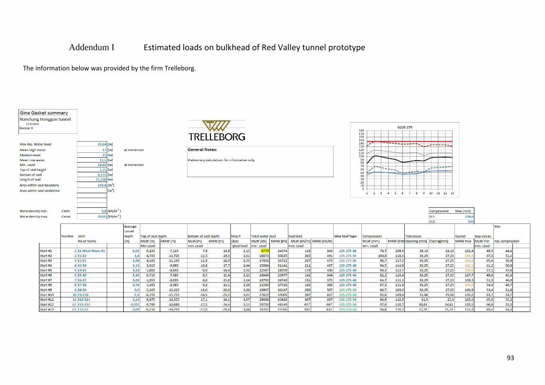
93

Addendum I Estimated loads on bulkhead of Red Valley tunnel prototype

The information below was provided by the firm Trelleborg.

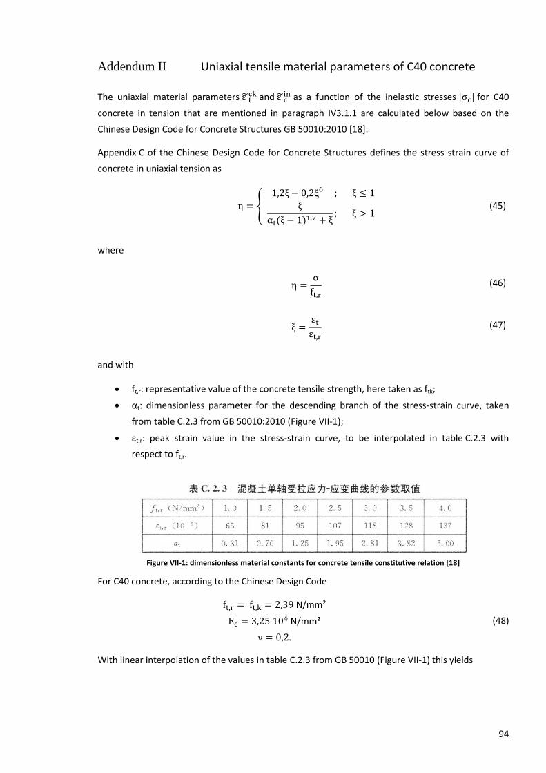
94

Addendum II Uniaxial tensile material parameters of C40 concrete

The uniaxial material parameters and

as a function of the inelastic stresses for C40

concrete in tension that are mentioned in paragraph IV3.1.1 are calculated below based on the

Chinese Design Code for Concrete Structures GB 50010:2010 [18].

Appendix C of the Chinese Design Code for Concrete Structures defines the stress strain curve of

concrete in uniaxial tension as

(45)

where

(46)

(47)

and with

ft,r: representative value of the concrete tensile strength, here taken as ftk;

αt: dimensionless parameter for the descending branch of the stress-strain curve, taken

from table C.2.3 from GB 50010:2010 (Figure VII-1);

εt,r: peak strain value in the stress-strain curve, to be interpolated in table C.2.3 with

respect to ft,r.

Figure VII-1: dimensionless material constants for concrete tensile constitutive relation [18]

For C40 concrete, according to the Chinese Design Code

N/mm²

N/mm²

(48)

With linear interpolation of the values in table C.2.3 from GB 50010 (Figure VII-1) this yields

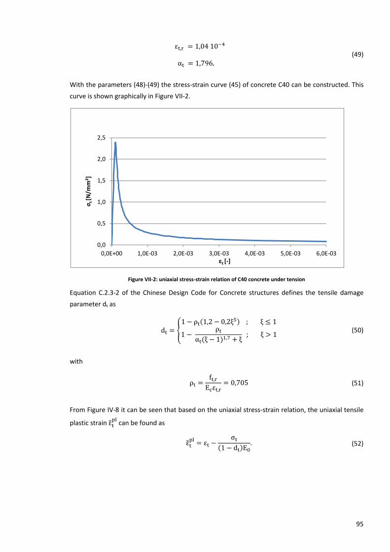
95

(49)

With the parameters (48)-(49) the stress-strain curve (45) of concrete C40 can be constructed. This

curve is shown graphically in Figure VII-2.

Figure VII-2: uniaxial stress-strain relation of C40 concrete under tension

Equation C.2.3-2 of the Chinese Design Code for Concrete structures defines the tensile damage

parameter dt as

(50)

with

(51)

From Figure IV-8 it can be seen that based on the uniaxial stress-strain relation, the uniaxial tensile

plastic strain

can be found as

(52)

0,0

0,5

1,0

1,5

2,0

2,5

0,0E+00 1,0E-03 2,0E-03 3,0E-03 4,0E-03 5,0E-03 6,0E-03

σt [N

/mm

²]

εt [-]

96

Once

is known through equation (52), the cracking strain can be found by using equation

(14) from paragraph IV3.1.1:

(14)

or, alternatively by reasoning on the stress-strain relation in Figure IV-8:

(53)

By using the stresses and strains from the constitutive relation (45) together with equation (50)-(53)

the tensile stress in the inelastic region in function of the cracking strain is found. The inelastic

tensile stress σt and the cracking strain in function of a number of tensile strain values is

mentioned in Table VII-1. These are the values that are mentioned in Table IV-4 in paragraph

IV3.1.1.

Table VII-1: uniaxial elastic strains in function of inelastic stresses

εt [-] σt [N/m²] [-]

1,04E-04 2,39 0

3,20E-04 0,79 2,96E-04

5,60E-04 0,47 5,46E-04

1,40E-03 0,22 1,39E-03

2,00E-03 0,17 1,99E-03

5,00E-03 0,09 5,00E-03

97

Addendum III Evolution of maximal principal plastic strain in concrete

shear keys numerical model at Ff = 360 kN

99

Addendum IV Evolution of tensile equivalent plastic strain

in

concrete shear keys numerical model at Ff = 360 kN

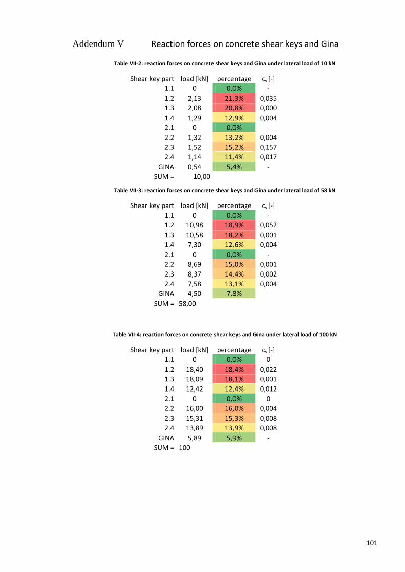
101

Addendum V Reaction forces on concrete shear keys and Gina

Table VII-2: reaction forces on concrete shear keys and Gina under lateral load of 10 kN


1.1 0 0,0% -

1.2 2,13 21,3% 0,035

1.3 2,08 20,8% 0,000

1.4 1,29 12,9% 0,004

2.1 0 0,0% -

2.2 1,32 13,2% 0,004

2.3 1,52 15,2% 0,157

2.4 1,14 11,4% 0,017

GINA 0,54 5,4% -

SUM = 10,00



1.1 0 0,0% -

1.2 10,98 18,9% 0,052

1.3 10,58 18,2% 0,001

1.4 7,30 12,6% 0,004

2.1 0 0,0% -

2.2 8,69 15,0% 0,001

2.3 8,37 14,4% 0,002

2.4 7,58 13,1% 0,004

GINA 4,50 7,8% -

SUM = 58,00



1.1 0 0,0% 0

1.2 18,40 18,4% 0,022

1.3 18,09 18,1% 0,001

1.4 12,42 12,4% 0,012

2.1 0 0,0% 0

2.2 16,00 16,0% 0,004

2.3 15,31 15,3% 0,008

2.4 13,89 13,9% 0,008

GINA 5,89 5,9% -

SUM = 100

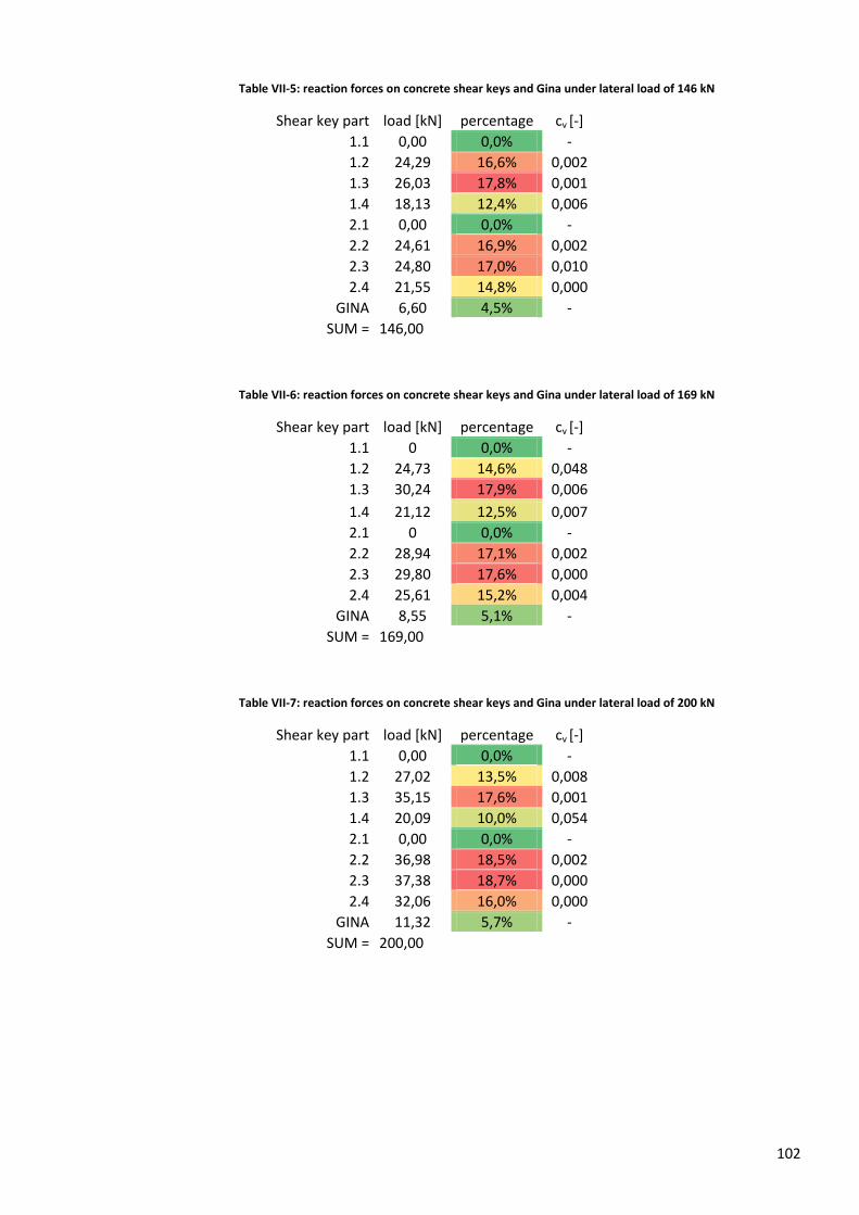
102



1.1 0,00 0,0% -

1.2 24,29 16,6% 0,002

1.3 26,03 17,8% 0,001

1.4 18,13 12,4% 0,006

2.1 0,00 0,0% -

2.2 24,61 16,9% 0,002

2.3 24,80 17,0% 0,010

2.4 21,55 14,8% 0,000

GINA 6,60 4,5% -

SUM = 146,00



1.1 0 0,0% -

1.2 24,73 14,6% 0,048

1.3 30,24 17,9% 0,006

1.4 21,12 12,5% 0,007

2.1 0 0,0% -

2.2 28,94 17,1% 0,002

2.3 29,80 17,6% 0,000

2.4 25,61 15,2% 0,004

GINA 8,55 5,1% -

SUM = 169,00



1.1 0,00 0,0% -

1.2 27,02 13,5% 0,008

1.3 35,15 17,6% 0,001

1.4 20,09 10,0% 0,054

2.1 0,00 0,0% -

2.2 36,98 18,5% 0,002

2.3 37,38 18,7% 0,000

2.4 32,06 16,0% 0,000

GINA 11,32 5,7% -

SUM = 200,00

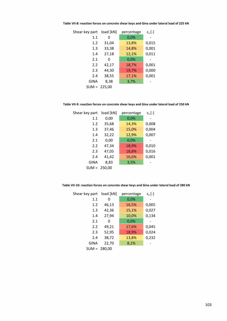
103



1.1 0 0,0% -

1.2 31,04 13,8% 0,015

1.3 33,38 14,8% 0,001

1.4 27,18 12,1% 0,011

2.1 0 0,0% -

2.2 42,17 18,7% 0,001

2.3 44,30 19,7% 0,000

2.4 38,55 17,1% 0,001

GINA 8,38 3,7% -

SUM = 225,00



1.1 0,00 0,0% -

1.2 35,68 14,3% 0,008

1.3 37,46 15,0% 0,004

1.4 32,22 12,9% 0,007

2.1 0,00 0,0% -

2.2 47,34 18,9% 0,010

2.3 47,05 18,8% 0,016

2.4 41,42 16,6% 0,001

GINA 8,83 3,5% -

SUM = 250,00



1.1 0 0,0% -

1.2 46,13 16,5% 0,005

1.3 42,36 15,1% 0,027

1.4 27,94 10,0% 0,134

2.1 0 0,0% -

2.2 49,21 17,6% 0,045

2.3 52,95 18,9% 0,024

2.4 38,72 13,8% 0,232

GINA 22,70 8,1% -

SUM = 280,00

structural behavior of concrete shear keys in the nanchang ... · structural behavior of concrete...

Documents