Final Report for Technical Assistance for an Ecological Evaluation of the Southwest Florida Feasibility Study

STRESSOR RESPONSE MODEL FOR Vallisneria americana

By Frank J. Mazzotti, Leonard G. Pearlstine, Robert H. Chamberlain, Melody J. Hunt, Tomma Barnes, Kevin Chartier, Alicia M. Weinstein, and Donald DeAngelis

Joint Ecosystem Modeling Laboratory

Technical Report Series

ii

FINAL REPORT

for

Technical Assistance for an Ecological Evaluation of the

Southwest Florida Feasibility Study

STRESSOR RESPONSE MODELS FOR Vallisneria americana

Prepared By: Frank J. Mazzotti1, Leonard G. Pearlstine1, Robert H. Chamberlain 2, Melody J. Hunt2, Tomma Barnes3,

Kevin Chartier1, and Donald DeAngelis4

1University of Florida Ft. Lauderdale Research and Education Center

3205 College Ave Davie, FL 33314 (954) 577-6304

2South Florida Water Management District

3301 Gun Club Road West Palm Beach, FL 33406

3Post, Buckley, Schuh and Jernigan

3501 North Causeway Blvd., Suite 725 Metairie, LA 70001

(504) 862-1481

4United States Geological Survey University of Miami, Dept. of Biology

1301 Memorial Dr. RM 215 Coral Gables, FL 33146

Prepared For: South Florida Water Management District

Fort Myers Service Center 2301 McGregor Blvd. Fort Myers, FL 33901

United States Geological Survey

1301 Memorial Dr. RM 215 Coral Gables, FL 33146

(305) 284-3974

November 2006

iii

University of Florida

This report should be cited as:

Mazzotti, F.J., Pearlstine, L.G., Chamberlain, R.H., Hunt, M.J., Barnes, T., and Chartier, K., and DeAngelis, D. 2006, Stressor response models for Vallisneria Americana.. JEM Technical Report 2006-06. Final report to the South Florida Water Management District and the U.S..Geological Survey. University of Florida, Florida Lauderdale Research and Education Center, Fort Lauderdale, Florida, 12 pages.

Any use of trade, firm, or product names is for descriptive purposes only and does not imply endorsement by the University of Florida.

Although this report is in the public domain, permission must be secured from the individual copyright owners to reproduce any copyrighted material contained within this report.

Contents Introduction ..................................................................................................................................... 1

Southwest Florida Feasibility Study ............................................................................................ 1 C43 West Reservoir ..................................................................................................................... 1

Forcasting Models ........................................................................................................................... 1 Habitat Suitability Indices............................................................................................................ 2

Ecology of Vallisneria americana ................................................................................................. 2 HSI for Vallisneria americana ..................................................................................................... 10

HSI Formula............................................................................................................................... 10 HSI Curves and Application ...................................................................................................... 10

References Cited............................................................................................................................ 16

Figures Figure 1. Caloosahatchee Estuary sampling area ......................................................................... 3 Figure 2. Field survey results of shoot counts vs. salinity ............................................................ 4 Figure 3. Tape grass in upper Caloosahatchee Estuary ................................................................ 4 Figure 4. Laboratory experimental results of growth rate vs. salinity .......................................... 5 Figure 5. Field survey results of shoot counts vs. inflow from S-79.......................................... ..6 Figure 6. HSI value for Vallisneria americana in response to salinity ...................................... 11 Figure 7. HSI value for Vallisneria americana response to average daily bottom light in

low salinity range .................................................................................................. 12 Figure 8. HSI value for Vallisneria americana response to average daily bottom light in

high salinity range ................................................................................................. 12 Figure 9. Equation to determine ADBL...................................................................................... 13 Figure 10. Average monthly incident PAR .................................................................................. 13 Figure 11. HSI relationship between average daily flow and K value ......................................... 14 Figure 12. HSI value for Vallisneria americana in response to temperature…………………... 15 Figure 13. Daily average temperature from historical records .…………………..……………. 15

Tables Table 1. Summary of freshwater inflow and water quality requirements for Vallisneria

americana in the Caloosahatchee estuary ..................................................................... 8 Table 2. Changes to HSI model's spatial boundaries and post processing routines ………..... 8

iv

STRESSOR RESPONSE MODEL FOR Vallisneria americana

By Frank J. Mazzotti, Leonard G. Pearlstine, Robert H. Chamberlain, Melody J. Hunt, Tomma Barnes, Kevin Chartier, and Donald DeAngelis

Introduction A key component in adaptive management of Comprehensive Everglades Restoration Plan

(CERP) projects is evaluating alternative management plans. Regional hydrological and ecological models will be applied to evaluate restoration alternatives and the results will be applied to modify management actions.

Southwest Florida Feasibility Study

The Southwest Florida Feasibility Study (SWFFS) is a component of the Comprehensive Everglades Restoration Plan (CERP). The SWFFS is an independent but integrated implementation plan for CERP projects and was initiated in recognition that there were additional water resource issues (needs, problems, and opportunities) within Southwest Florida not being addressed directly by CERP. The SWFFS identifies, evaluates, and compares alternatives that address those additional water resource issues in Southwest Florida. An adaptive assessment strategy is being developed that will create a system-wide monitoring program to measure and interpret ecosystem responses. The SWFFS provides an essential framework to address the health and sustainability of aquatic systems. This includes a focus on water quantity and quality, flood protection, and ecological integrity.

C43 West Reservoir The purpose of the C43 Basin Storage Reservoir project is to improve the timing, quantity,

and quality of freshwater flows to the Caloosahatchee River estuary. The project’s initial phase includes an above-ground reservoir with a total water storage capacity of approximately 170,000 acre-feet and will be located in the C-43 Basin in Lee County. The initial design of the reservoir assumed 8094 hectares (20,000 acres) with water levels fluctuating up to 2.4 meters (8 feet) above grade. The final size, depth and configuration of this facility will be determined through more detailed planning and design.

Forecasting Models Forecasting models bring together research and monitoring to ecosystems of Southwest

Florida and place them into an adaptive management framework for the evaluation of alternative plans. There are two principle ways to structure adaptive management: (1) passive by which policy decisions are made based on a forecasting model and the model is revised as monitoring data

1

become available, and (2) active by which management activities are implemented through statistically valid experimental design to better understand how and why natural systems respond to management (Wilhere 2002).

In an integrated approach that includes both passive and active-adaptive management, a forecasting model simulates system response and is validated by monitoring programs to measure actual system response. Monitoring can then provide information for passive-adaptive management for recalibration of the forecasting model. Directed research, driven by model uncertainties, is an active-adaptive management strategy for learning and the reduction of uncertainties in the model.

The forecasting models for the C-43 West Reservoir Project and the Southwest Florida Feasibility Study consist of a set of stressor response (habitat suitability) models for individual species. These stressor response models have been developed principally with literature, expert knowledge, and currently available field data.

Habitat Suitability Indices Habitat Suitability Index (HSI) models were developed with each stressor variable

portrayed spatially and temporally across systems of the study area at scales appropriate to the organism or community being portrayed. The HSI models have been incorporated into a GIS to portray responses spatially and temporally to facilitate policy decisions. That is, the model describes a response surface of habitat suitability values that vary spatially according to stressor levels throughout the estuary and temporally according to temporal patterns in stressor variables. Much of the temporal variation is a result of temporal cycling of important stressor inputs, such as water temperature and salinity. Temporal change for other important variables may not be cyclical, such as rising sea level and increasing land use and fresh water demands in the region. Areas predicted to be suitable and those predicted to be less suitable or disturbed should be targeted for additional sampling as part of the model validation and adaptive management process.

Species selected for modeling (focal species) are ecologically, recreationally or economically important and have a well-established linkage to stressors of management interest. They may also make good focal species because they engage the public in caring about the outcome of restoration projects. The habitat suitability models (HSI) models were developed by choosing specific life stages of each species with the most limited, restricted, or tightest range of suitable conditions, to capture the highest sensitivities of the organisms to the environmental changes associated with the planned restoration activities. Values used in the models are listed in Table 1.

The models calculate habitat suitability monthly as the weighted geometric mean of the environmental variables identified as important for each model. Because the geometric mean is derived from the product of the variables rather than the sum (as in the arithmetic mean) and has the appropriate property that if any of the individual variables are unsuitable for species success (i.e., the value of the variable is zero) then the entire index goes to zero.

Ecology of Vallisneria americana One of the factors contributing to high productivity in estuaries has been the historic abundance of submerged aquatic vegetation (SAV). SAV also provide food for waterfowl and are critical habitat for shellfish and finfish. In addition, submerged plants affect nutrient cycling, sediment stability, and water clarity (Batiuk et al. 1992). Because SAV beds provide habitat for

2

benthic and pelagic organisms, many of their water chemistry requirements overlap, including preferred salinity and temperature ranges. However, SAV also serve well as indicators of water clarity and nutrient levels. Habitat requirements developed for fish and birds do not normally incorporate these conditions. In addition, “many of the restoration goals for fish and birds involve changes in both environmental quality and management of human harvesting activities” (Dennison et al. 1993). In contrast, SAV goals can more directly be linked to environmental and water quality, thus providing for more direct establishment of targets and protection goals in areas of the estuary where SAV are located (Batiuk et al. 1992, Dennison et al. 1993, Doering et al. 2002).

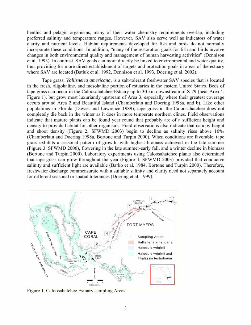
Tape grass, Vallisneria americana, is a salt-tolerant freshwater SAV species that is located in the fresh, oligohaline, and mesohaline portion of estuaries in the eastern United States. Beds of tape grass can occur in the Caloosahatchee Estuary up to 30 km downstream of S-79 (near Area 4: Figure 1), but grow most luxuriantly upstream of Area 3, especially where their greatest coverage occurs around Area 2 and Beautiful Island (Chamberlain and Doering 1998a, and b). Like other populations in Florida (Dawes and Lawrence 1989), tape grass in the Caloosahatchee does not completely die back in the winter as it does in more temperate northern clines. Field observations indicate that mature plants can be found year round that probably are of a sufficient height and density to provide habitat for other organisms. Field observations also indicate that canopy height and shoot density (Figure 2; SFWMD 2003) begin to decline as salinity rises above 10‰ (Chamberlain and Doering 1998a, Bortone and Turpin 2000). When conditions are favorable, tape grass exhibits a seasonal pattern of growth, with highest biomass achieved in the late summer (Figure 3, SFWMD 2006), flowering in the late summer-early fall, and a winter decline in biomass (Bortone and Turpin 2000). Laboratory experiments using Caloosahatchee plants also determined that tape grass can grow throughout the year (Figure 4; SFWMD 2003) provided that conducive salinity and sufficient light are available (Barko et al. 1984, Bortone and Turpin 2000). Therefore, freshwater discharge commensurate with a suitable salinity and clarity need not separately account for different seasonal or spatial tolerances (Doering et al. 1999).

Figure 1. Caloosahatchee Estuary sampling Areas

S-79

CAL

OO

SAH

ATC

HEE

RIVER

BAYSAN CARLOS

CORALCAPE

FORT MYERS

BAYESTERO

SHELLPOINT

BEAUTIFULISLAND

SANIBEL

ORANGE RIVER

5

6

4

7

3

2

Sampling Areas

1

42 6Kilom eters

0

Thalassia testud inumHalodule wrightii and

Vallisneria am ericanaHalodule wrightii

3

Vallisneria and Salinity

Salinity (o/oo)

0

200

400

600

800

1000

1200

1400

Figure 2. Field survey results of shoot counts vs. salinity (SFWMD 2003).

Vallisneria at Sites 1 & 2 Jan. 1998 - Mar. 2006

Date1/1/98 1/1/99 1/1/00 1/1/01 1/1/02 1/1/03 1/1/04 1/1/05 1/1/06

Salin

ity p

pt

0

4

8

12

16

20

24

28

Shoo

ts/m

2

0

200

400

600

800

1000

1200

Salinity (30-day moving average at

the Ft. Myers surface sensor).

------- Salinity (upper target limit).Station 1Station 2

WY2006

Figure 3. Tape grass (Vallisneria americana) shoot density in the upper Caloosahatchee Estuary (Sites 1 and 2 in Area 2, Figure 1). Recent data are from stations monitored by the Sanibel-Captiva Conservation Foundation and Mote Marine Laboratory (SFWMD 2006).

0 5 10 15 20 25 30

Sho

ots

m-2

Vallisneria and Salinity

Salinity (o/oo)

0

200

400

600

800

1000

1200

1400S

hoot

s m

-2

0 5 10 15 20 25 30

4

Vallisneria Blades

SalinitFigure 4. Laboratory experimental results of growth rate vs. salinity (SFWMD 2003).

General non-quantitative observations of tape grass during 1956-1989 found that relative abundance greatly varied annually throughout its range (Chamberlain et al. 1995) and indicated that healthy plants during the winter dry season lead to good coverage, taller plants, and reproduction during the peak summer growing months. Quantitative sampling since 1998 confirms this observation (Bortone and Turpin 2000).

In the upper estuary, temporal and spatial fluctuation in salinity and other important water quality parameters are largely driven by freshwater discharge at S-79. During periods of high discharge, usually during the summer wet season, the system turns fresh. During periods of low discharge during the winter and spring, salt water intrudes up the estuary.

Literature information, field studies, and laboratory investigations of tape grass salinity tolerance (SFWMD 2003) was used to establish hydrologic targets for developing the Minimum Flow and Level Rule (as per Florida Administrative Code, Section 40E-8.021(24)). After analysis of historical salinity records from the estuary along with an initial salinity model, a flow of 300 cfs from S-79 (Figure 5) was identified as the average minimum flow needed (SFWMD 2003) to support tape grass growth in the critical region of the estuary where it has historically been most abundant (Figure 1; Area 2). This designated flow volume, along with about 200 cfs input from the tidal tributaries and ground water, should maintain salinity at < 10‰ under average conditions and support tape grass growth. The MFL rule includes two salinity criteria measured near the Ft. Myers Yacht Basin (near Area 3, Figure 1). An MFL exceedence occurs if: (1) the 30-day moving average salinity rises above 10‰; or (2) a single daily average salinity rises above 20‰. The first criterion recognizes that tape grass in the critical region (Figure 1: Area 2) grows well at salinity below 10‰. The second accounts for the effect of exposure to high salinity for short time periods. Upon additional consideration and analysis (Chamberlain 2005, Chamberlain and Doering 2004), a

y Treatment0 5 10 15 20 25 30 35Ex

pone

ntia

l Gro

wth

r (d

-1)

-0.30-0.25-0.20-0.15-0.10-0.050.000.050.10

1/5/19985/20/20013/1/19967/11/1996

Vallisneria Blades

Salinit

Exp

onen

tial G

row

th r

(d-1

)

-0.30-0.25-0.20-0.15-0.10-0.050.000.050.10

y Treatment

1/5/19985/20/20013/1/19967/11/1996

0 5 10 15 20 25 30 35

5

minimum flow of 450 cfs is now promoted to better insure tape grass protection during very dry conditions when the tidal tributary flow contribution is diminished well below the required 200 cfs.

Vallisneria Shoots

30-Day Average Discharge at S-79 (CFS)

0 2000 4000 6000 8000 10000

Sho

ots

/ m2

0

200

400

600

800

1000

1200

1400

300 CFS

Figure 5. Field survey results of shoot counts vs. inflow from S-79 (Doering et al. 2002, SFWMD 2003).

Although viable rosettes (short immature plants) are almost always present, total denuding of the bottom and loss of all plants can occur. This situation became evident after the year 2000 drought (Figure 3). Plants did not return in appreciable numbers after 2 years, thus confirming significant harm to this portion of the estuary as defined by the MFL Rule (SFWMD 2003).

Doering et al. (1999) reported decreasing growth of tape grass as salinity increased (Figure 3) whereby positive growth became zero when salinity exceeded 10‰. Doering et al. (1999) also found that tape grass survived at 15‰ for over 40 days under ample light conditions and mortality was observed at 18‰, with a few viable plants persisting after 70 days (Doering et al., 2001). Analysis of long-term records reveals saltwater intrusion into the upper estuary that results in salinity of >10‰ may last for over 100 days, but almost always is less than 70 days. Median durations are 5-12 days. Therefore, approximately 50% of the intrusion events that occur may last long enough to impact tape grass growth. Peak salinities during these intrusion average 13-14‰, which is near the tape grass limit for growth, but approximately 25% of the peak salinities are >18‰, which can severely reduced coverage and bed morphometrics (Kraemer et al. 1999, Doering et al. 2001). During a field experiment in the Caloosahatchee Estuary, Kraemer et al (1999) found that exposure to salinities approaching 18‰ for longer than 2 weeks - 1 month resulted in tape grass mortality from which plants did not recover. Based on the results of studies and information

6

discussed above, the HSI curve in Figure 6 was formulated for a model described in Hunt and Doering (2005).

Both long term and short term exposures (if repeated) during the late winter may result in tape grass not fulfilling its growth potential needed to provide habitat during the spring and summer season. In addition, other growth parameters, such as water clarity and temperature can also influence contiguous plant coverage and recovery after population declines. Therefore, rules were developed (Table 2) for applying to the HSI model, in order to insure previous conditions are considered when determining the new HSI value each month.

Research to date indicates that the flow distributions specified by Chamberlain and Doering (2004) should promote good water quality (Doering and Chamberlain 1998, Chamberlain et al. 2003) in the ranges suggested by Dennison et al. (1993). The numeric tape grass model developed by Hunt and Doering (2005) uses salinity, light attenuation, and temperature as independent variables to predict tape grass density. The model confirms that light is an important variable for tape grass growth in the Caloosahatchee. Even though high flows are not a concern for tape grass regarding salinity, they are associated with reduced plant density (Figure 5). Water clarity decreases during increased flows due to suspended solids, color and in some cases increased incident of algal blooms. These factors may contribute to a decrease in tape grass growth, recovery, distribution along the estuary, and the depth it can survive.

Batiuk et al. (1992) and Dennison et al. (1993) reviewed water quality requirements for SAV that are found in estuaries and suggested guideline values for water clarity, suspended solids, nutrients, and chlorophyll-a for tape grass (Table 1). In the field transplant studies by Kraemer et al. (1999), salinity tolerances appeared lower than in laboratory experiments, and it was suggested that other factors, particularly light co-varying with salinity can influence the distributional limits. Further evidence of the importance of light in this ecosystem was reported by Bortone and Turpin (2000). In a field study, they found V. americana biomass to be significantly associated with six factors: location, temperature, depth, secchi depth, TSS and color – making four of the six factors associated with light conditions. Additional laboratory mesocosm experiments were conducted to quantify the effects of light stress at different salinities (Hunt et al, 2003; 2004). Photosynthesis/ Irradiance (P/I) curves were developed and showed that light utilization varies with salinity. Based on this work by Hunt et al. (2003; 2004), two HSI curves were developed for different ranges of salinity. Figure 7 and 8 depict the index values for tape grass response to average daily bottom light (ADBL) when salinity is < 9.5‰ and >9.5‰, respectively. Figure 9 provides the formula for calculating ADBL, which requires knowing (1) incident light in the PAR (Photosynthetic Active Radiation) spectral range; (2) water column light attenuation (K); and (3) depth. Average monthly incident PAR for the Caloosahatchee is depicted in Figure 10 and was calculated from a daily average PAR dataset, recorded by a continuous sensor during 1998-2004, located in the nearby Estero Bay Watershed. Light attenuation was calculated based on freshwater inflow from S-79 (resulting regression line-Figure 11). This relationship was determined from analysis that predicted secchi disk readings (dependent variable) from the 30-day average S-79 flow volume (cfs). Average daily flow is recorded by the USGS since structure 1965 and the secchi disk data to support the regression analysis came from field measurements collected intermittently since 1986. Light attenuation (K) is calculated form the predicted secchi value by the formula, -1.65/secchi (Batiuk et al. 1992). Depth was determined from bathymetry surveys of the Caloosahatchee Estuary and the resulting information supplied in a GIS data file that matched the grid cell points of the model.

7

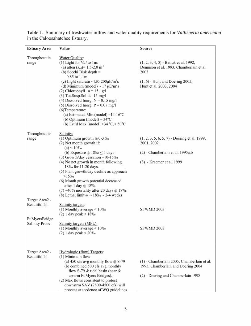
Table 1. Summary of freshwater inflow and water quality requirements for Vallisneria americana in the Caloosahatchee Estuary. Estuary Area Value Source Throughout its range

Water Quality: (1) Light for Val to 1m: (a) atten (Kd)= 1.5-2.0 m-1 (b) Secchi Disk depth = 0.85 to 1.1m (c) Light saturatn ~150-200μE/m2s (d) Minimum (model) ~ 17 μE/m2s (2) Chlorophyll –a = 15 µg/l (3) Tot.Susp.Solids=15 mg/l (4) Dissolved Inorg. N = 0.15 mg/l (5) Dissolved Inorg. P = 0.07 mg/l (6)Temperature: (a) Estimated Min.(model) ~14-16oC (b) Optimum (model) ~ 34oC (b) Est’d Max.(model) >34 oC,< 50oC

(1, 2, 3, 4, 5) - Batiuk et al. 1992, Dennison et al. 1993, Chamberlain et al. 2003 (1, 6) - Hunt and Doering 2005, Hunt et al. 2003, 2004

Throughout its range Target Area2 - Beautiful Isl. Ft.MyersBridge Salinity Probe

Salinity: (1) Optimum growth @ 0-3 ‰ (2) Net month growth if: (a) < 10‰ (b) Exposure @ 18‰ < 5 days (3) Growth/day cessation ~10-15‰ (4) No net growth in month following 18‰ for 11-20 days. (5) Plant growth/day decline as approach >15‰ (6) Month growth potential decreased after 1 day @ 18‰ (7) ~40% mortality after 20 days @ 18‰ (8) Lethal limit @ ~ 18‰ ~ 2-4 weeks Salinity targets: (1) Monthly average < 10‰ (2) 1 day peak < 18‰ Salinity targets (MFL): (1) Monthly average < 10‰ (2) 1 day peak < 20‰

(1, 2, 3, 5, 6, 5, 7) - Doering et al. 1999, 2001, 2002 (2) - Chamberlain et al. 1995a,b (8) - Kraemer et al. 1999 SFWMD 2003 SFWMD 2003

Target Area2 - Beautiful Isl.

Hydrologic (flow) Targets: (1) Minimum flow (a) 450 cfs avg monthly flow @ S-79 (b) combined 500 cfs avg monthly flow S-79 & tidal basin (near & upstrm Ft.Myers Bridges). (2) Max flows consistent to protect downstrm SAV (2800-4500 cfs) will prevent exceedence of WQ guidelines.

(1) - Chamberlain 2005, Chamberlain et al. 1995, Chamberlain and Doering 2004 (2) - Doering and Chamberlain 1998

8

(3) Defined preferred flow distribution (EST05) that maximizes flows (75%) in 450-800 cfs range will maximize WQ for growth

(3) – Chamberlain et al. 2003

Target Area2 - Beautiful Isl.

Target Plant Morphometricts (June-Sept growing season): (1) Minimum 20% of average potential shoot density (~200-300 shoots/m2 of potential > 1,000 shts/m2). (2) Minimum avg. blade length 15cm (3) Most years > 500-600 shts/m2 (4) Most years-plant reproduction (sexual) (5) Run tape grass model to evaluate/select preferred flows

(1, 2) Chamberlain 2005, Chamberlain et al. 2003 (3) - SFWMD 2006 (4) - Doering et al. 1999, 2002 (5) - Hunt et al. 2003, 2004, 2005

Temperature is an additional factor that may influence tape grass growth. In general,

temperature changes primarily influence growth of SAV over predictable seasonal cycles. In northern environments there is a distinct seasonal growth pattern involving the production of vegetative tubers and winter dormancy period during the cold winter months. Different temperature growth ranges have been reported for V. americana in populations growing in different climates and under different environmental conditions. Titus and Adams (1979) report a temperature optimum for V. americana obtained from University Bay, Madison, WI. of 32.6oC. In the Detroit River, V. americana grew at water temperatures ranging from 19 to 31.5 oC (Hunt 1963). Barko et al. (1982, 1984) reported growth of commercially obtained juvenile plants was severely restricted below 20oC.

Consistent with the southern ecotype of V. americana reported by Smart and Dorman (1993), no over-wintering buds or tubers have been reported in the Caloosahatchee Estuary. The acute limits or effects of the colder winter water temperatures on the growth and survival in Florida is not known. Water temperatures in the upper Caloosahatchee Estuary over the period 1998-2005 have varied between 14oC in the winter to 34oC in the summer. Inter-annual variation in seasonal high and low water temperatures are also apparent over this time period. Lower water temperature during some years may adversely impact tape grass. High freshwater inflow that increases water color may result in dark water that absorbs solar energy and raises water temperature near tape grass tolerance limits. Given the span in water temperatures in the Caloosahatchee Estuary, ranging from potentially above optimal conditions to below tolerance levels in any given year and the importance of over-wintering survival, water temperature may be an important variable that influences V. americana survival

A habitat suitability temperature curve (Figure 12) was developed for tape grass in the Caloosahatchee based on an equation of O'Neill et al. (1972). Input values for the lower lethal, optimum, and upper lethal limits came from general literature values (not specific to Florida) and calibrated based on a growth model described by Hunt and Doering (2005). Non-linear regression was employed to predict daily average temperature in the Caloosahatchee Estuary using historical data collected by continuous sensors since 1992 (Figure 13). Note, that as a daily average data set predicted from historical records, it does not reflect the high or low conditions that might be expected in any given year.

9

HSI for Vallisneria americana

HSI Formula Calculated monthly: HSI = (Previousw * Salinityw * Light Availability * Temperaturew) Previous "Previous" variable included because current month’s HSI score should depend on the how well the grass was doing last month (previous score). Previous = previous_month_HSI score + 0.05 (not to exceed 1.0), in order to allow for

growth from month to month if other conditions are suitable.

Table 2. Changes to HSI model’s spatial boundaries (A) and post-processing routines (B and C) for adjusting the final HSI ecological model scores to better reflect long-term impacts of severe reduction in Vallisneria americana density due to low HSI scores of environmental variables (salinity, light and temperature in above model formula).

Routine Model output criteria Model score adjustment A. Establish a lower depth threshold of 5 ft Model areas > 5 feet are not scored B. If HSI score < 0.2 for one month, Than HSI remains <0.2 for remainder of the season C. If HSI score < 0.1 for one month, Than HSI = 0 for 12 subsequent months Adjustments were agreed to by ecological benefits sub-team (6/14/06)

HSI Curves and Application (for determining input values to HSI model formula) Salinity

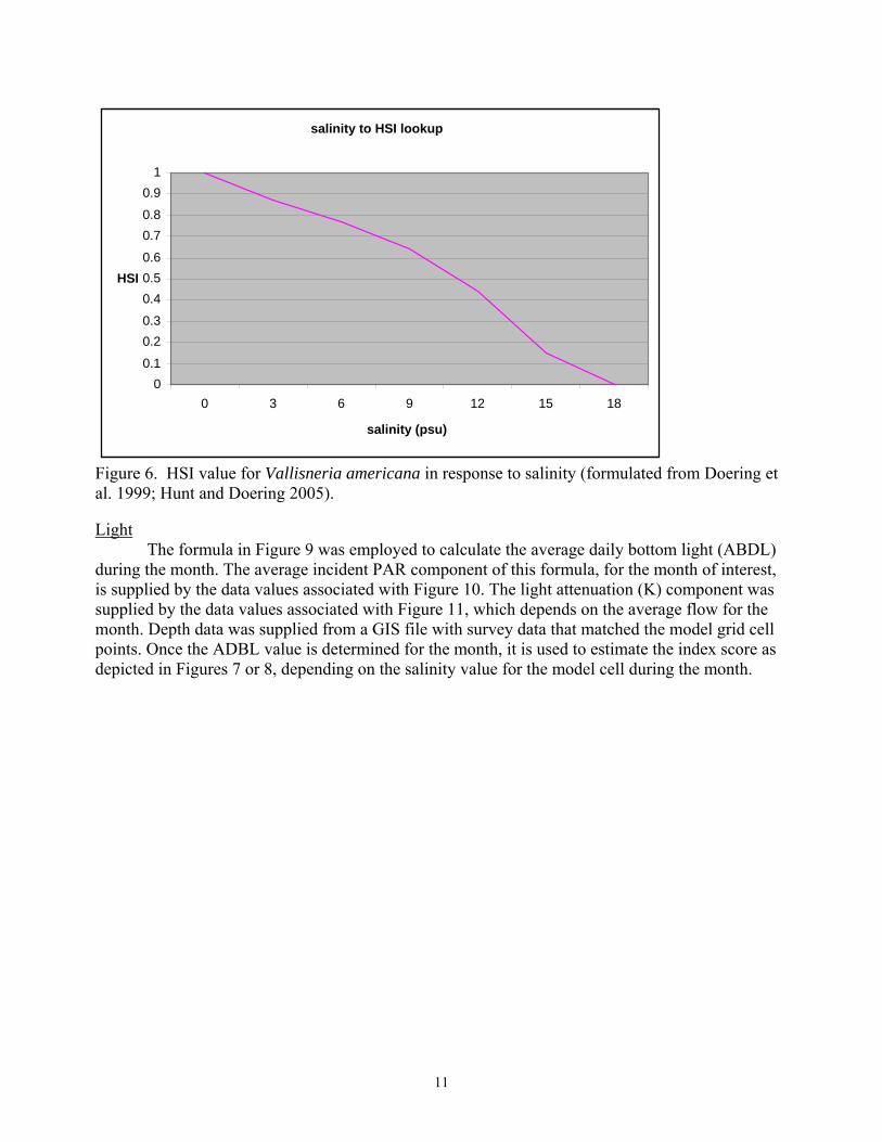
The freshwater inflow associated with base conditions and management alternatives serve as input for the hydrodynamic model (CH3D with regression routine) that estimates salinity concentration at key locations in the estuary. An immolator program used the salinity output to further estimate salinity at the remaining model grid cells. This salinity was compared to the curve in Figure 6 to determine the HSI score for that grid cell and input to the model formula.

10

salinity to HSI lookup

0 0.1 0.2 0.3 0.4 0.5 0.6 0.7 0.8 0.9

1

0 3 6 9 12 15 18

salinity (psu)

HSI

Figure 6. HSI value for Vallisneria americana in response to salinity (formulated from Doering et al. 1999; Hunt and Doering 2005).

Light

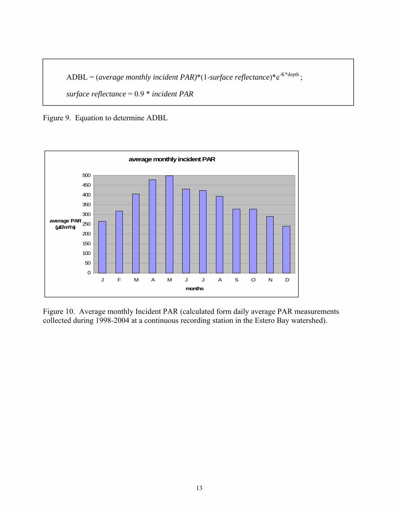
The formula in Figure 9 was employed to calculate the average daily bottom light (ABDL) during the month. The average incident PAR component of this formula, for the month of interest, is supplied by the data values associated with Figure 10. The light attenuation (K) component was supplied by the data values associated with Figure 11, which depends on the average flow for the month. Depth data was supplied from a GIS file with survey data that matched the model grid cell points. Once the ADBL value is determined for the month, it is used to estimate the index score as depicted in Figures 7 or 8, depending on the salinity value for the model cell during the month.

11

Figure 7. HSI value for Vallisneria response to average daily bottom light in low salinity range (<9.5psu) conditions (Hunt et al. 2004 and 2003; Hunt and Doering, 2005).

ADBL to HSI lookup, low salinity (<9.5psu)

0

0.1

0.2

0.3

0.4

0.5

0.6

0.7

0.8

0.9

1

17 40 90 136 192 387 average ADBL (µE/m²/s)

HSI

ADBL to HSI lookup, high salinity (>=9.5psu)

0

0.1

0.2

0.3

0.4

0.5

0.6

0.7

0.8

0.9

1

17 49 97 170 300

average ADBL (µE/m²/s)

HSI

Figure 8. HSI value for Vallisneria response to average daily bottom light in low salinity range (>9.5psu) conditions (Hunt et al. 2004 and 2003; Hunt and Doering, 2005).

12

ADBL = (average monthly incident PAR)*(1-surface reflectance)*e-K*depth ;

surface reflectance = 0.9 * incident PAR Figure 9. Equation to determine ADBL

average monthly incident PAR

0

50

100

150

200

250

300

350

400

450

500

J F M A M J J A S O N D

months

average PAR (µE/m²/s)

Figure 10. Average monthly Incident PAR (calculated form daily average PAR measurements collected during 1998-2004 at a continuous recording station in the Estero Bay watershed).

13

flow to K lookup, Vallisneria

8

7

6

5

4K

3

2

1

0 00 15100 15900 700 0 2300 3100 3900 4700 55000 80

Figure 11. HSI relationship between average daily flow and light attenuation (K values).

Temperature

Daily average temperature was estimated from continuous in-water recorders that have been measuring near surface temperature since 1992. Depending on the HSI model requirements, these daily values (Figure 13) can be averaged over the time period of interest (e.g., monthly average). The resulting temperature is then used to determine the index value in Figure 12 for input to the HSI model formula.

150 630071007900870095001030011100119001270013500143

average daily flow (cubic feet per minute)

14

Temperature to HSI lookup

1 0.9 0.8 0.7 0.6

Figure 12. HSI value for Vallisneria in response to temperature (O'Neill et al., 1972, Hunt and Doering 2005).

Predicted Daily Temperature

Day of Year0 30 60 90 120 150 180 210 240 270 300 330 360

Tem

pera

ture

(o C)

1617181920212223242526272829303132

Day of Year vs Predicted Shallow Temp @ S-79 Day of Year vs Predicted Shallow Temp @ Br-31 Day of Year vs Predicted Shallow Temp @ FtM Day of Year vs Predicted Shallow Temp @ Shell Pt. and Sanibel Causeway

Figure 13. Daily average temperature estimated from historical records in the Caloosahatchee.

0 0.1 0.2 0.3 0.4 0.5

48 50

temperature (ºC)

HSI

14 16 18 20 22 24 26 28 30 32 34 36 38 40 42 44 46

15

References Cited Chamberlain, R.H. 2005. C-43 Basin Storage Reservoir Project - Caloosahatchee Estuary Hydrologic Evaluation Performance Measures. C-43 BSR Study Team Adopted Draft, June 28, 2005. Chamberlain, R. H. and P.H. Doering. 1998a. Freshwater inflow to the Caloosahatchee Estuary and the resource-based method for evaluation, p. 81-90. In S.F. Treat (ed.), Proceedings of the 1997 Charlotte Harbor Public Conference and Technical Symposium. South Florida Water Management District and Charlotte Harbor National Estuary Program, Technical Report No. 98-02. Washington, D.C. Chamberlain, R. H. and P.H. Doering. 1998b. Preliminary estimate of optimum freshwater inflow to the Caloosahatchee Estuary: A resource-based approach, p. 121-130. In S.F. Treat (ed.), Proceedings of the 1997 Charlotte Harbor Public Conference and Technical Symposium. South Florida Water Management District and Charlotte Harbor National Estuary Program, Technical Report No. 98-02. Washington, D.C. Chamberlain, R. H. and P.H. Doering. 2004. Recommended Flow Distribution (the Caloosahatchee Estuary and the C-43 basin Storage Reservoir Project). Technical Memorandum, South Florida Water Management District. Chamberlain, R.H., P.H. Doering, and K.M. Haunert. 2003. Preliminary assessment of water quality and material loading in the Caloosahatchee Estuary, FL. Poster Presentation, 17th Biennial Conference of the Estuarine Research Federation. Chamberlain, R.H., D.E. Haunert, P.H. Doering, K.M. Haunert, and J.M. Otero. 1995. Preliminary estimate of optimum freshwater inflow to the Caloosahatchee Estuary, Florida. Technical report, South Florida Water Management District, West Palm Beach, Florida Barko, J. W., D. G. Hardin and M. S. Matthews. 1982. Growth and morphology of submerged freshwater macrophytes in relation to light and temperature. Canadian J. Bot. 60:877-887 Barko, J. W., D. G. Hardin, and M. S. Matthews. 1984. Interactive Influences of Light and Temperature on the Growth and Morphology of Submerged Freshwater Macrophytes. Technical Report A-84-3, U. S. Army Corps of Engineers, Waterways Experimental Station, Vicksburg, Miss. 24 pp. Batiuk, R.A., R.J. Orth, K.A. Moore, W.C. Dennison, J.C. Stevenson, L.W. Staver, V. Carter, N.B. Rybicki, R.E. Hickman, S. Kollar, S. Bieber, and P. Heasly 1992. Chesapeake Bay submerged aquatic vegetation habitat requirements and restoration targets: A technical synthesis. Chesapeake Bay Program CBP/TRS 83/92 186 pp. Bortone, S.A., and R.K. Turpin. 2000. Tape grass life history metrics associated with environmental variables in a controlled estuary. In: Bortone, S.A. (ed.), Seagrasses: Monitoring, Ecology, Physiology, and Management. CRC Press, Boca Raton, Florida, pp. 65-79.

16

Dawes, C. J. and J. M. Lawrence. 1989. Allocation of energy resources in the freshwater angiosperms Vallisneria americana Michx. and Potomogeton pectinatus L. in Florida. Florida Scientist. Volume 52: pp 59 - 63. Dennison, W.C., R.J. Orth, K.A. Moore, J.C. Stevenson, V. Carter, S. Kollar, P. W. Bergstrom and R.A. Batiuk. 1993. Assessing water quality with submersed aquatic vegetation. Bioscience 43(2):86-94. Doering, P.H. and R.H. Chamberlain 1998. Water quality in the Caloosahatchee Estuary, San Carlos Bay and Pine Island Sound. Proceedings of the Charlotte Harbor Public Conference and Technical Symposium; 1997 March 15-16; Punta Gorda, FL. Pp 229-240. Charlotte Harbor National Estuary Program Technical Report No. 98-02. 274 p. Doering, P. H., R. H. Chamberlain, K. M. Donohue, and A. D. Steinman. 1999. Effect of salinity on the growth of Vallisneria americana Michx. from the Caloosahatchee Estuary, Florida. Florida Scientist. Vol. 62, No.2. pp. 89-105 Doering, P. H., R. H. Chamberlain, and D.E. Haunert. 2002. Using submerged aquatic vegetation to establish minimum and maximum freshwater inflows to the Caloosahatchee Estuary, Florida. Estuaries 25 (1343-1354). Doering, P. H., R. H. Chamberlain, and J. M. McMunigal. 2001. Effects of simulated saltwater intrusions on the growth and survival of wild celery, Vallisneria americana, from the Caloosahatchee Estuary (South Florida). Estuaries. Vol. 24. No. 6A, pp. 894-903. Hunt, G. S. 1963. Wild Celery in the lower Detroit River. Ecology 44:360-370 Hunt, M.J. 2003. An Ecological Model to Predict V. americana Densities in the Upper Caloosahatchee Estuary. In Proceedings of Greater Everglades Restoration Science Conference, Palm Harbor, FL. April 13-18. Hunt, M.J. and P.H. Doering. 2005. Significance of Considering Multiple Environmental Variables When Using Habitat as an Indicator of Estuarine Condition. In Bortone, S. A. (ed.), Estuarine Indicators, CRC Press, Boca Raton, Fl, pp.221-227. Hunt, M.J., P.H. Doering, R.H. Chamberlain, and K.M. Haunert. 2003. Light and Salinity Stress for SAV Determined by Modeling and Experimental Work in the Oligohaline Zone of an Estuary. In Proceedings of Estuarine Research Federation, Seattle, WA. September Hunt, M.J., P.H. Doering, R.H. Chamberlain, and K.M. Haunert. 2004. Grass Bed Growth and Estuarine Condition: Is size a Factor worth Considering? In Conference Proceedings of the Southeastern Estuarine research Society, Harbor Branch Oceanographic Institution, Fort Pierce, FL. April 15-17. Kraemer, G. P., R. H. Chamberlain, P. H. Doering, A. D. Steinman, and M. D. Hanisak. 1999. Physiological responses of transplants of the freshwater angiosperm Vallisneria americana along a

17

salinity gradient in the Caloosahatchee Estuary (Southwestern Florida). Estuaries. Vol. 22, No. 1 pp. 138-148. O'Neill, R.V., R. A. Goldstein, H. H. Shugart, and J.B. Manki. 1972. Terrestrial Ecosystem Energy Model. U.S. IBP Eastern Deciduous Forest Biome Memo Report 72-19 Oak Ridge National Laboratory, Oak Ridge, TN Smart, R. M., and J. D. Dorman. 1993. Latitudinal differences in the growth strategy of a submerged aquatic plant: ecotype differences in Vallisneria americana? Bull.Ecol. Soc. Am. 74 (Suppl.):439 South Florida Water Management District. 2003. Technical Documentation to Support Development of Minimum Flows and Levels for the Caloosahatchee River and Estuary, Status Update Report. May 2003. South Florida Water Management District. 2006. South Florida Environmental Report (Draft). Chapter 12 - Caloosahatchee River, Estuary, and Southern Charlotte Harbor. Titus, J. E. and M. S. Adams. 1979. Coexistence and the comparative light relations of the submerged macrophytes Myriophylulum spicatum L. and Vallisneria americana Michx. Oecologia. 40:273-286 Wilhere, G.F. 2002. Adaptive management in habitat conservation plans. Conserv. Biol. 16(1): 20-

29.

18

19