stress and seismic anisotropy near salt bodies – numerical...

EAGE 69th Conference & Exhibition — London, UK, 11 - 14 June 2007

C016Stress and Seismic Anisotropy Near Salt Bodies –Numerical Modeling and Observation from Wide-Azimuth Marine DataR. Bachrach* (WesternGeco), M. Sengupta (WesternGeco) & A. Salama(WesternGeco)

SUMMARYWide-azimuth marine data enable us to observe and analyze the azimuthal response of marine sediments.Modeling the stress near salt bodies using realistic salt geometry and a finite-element solver, we show thatthe presence of salt bodies cause changes in the orientation of the stress in the sediment near the salt. Thus,horizontal stresses magnitude and direction may vary near salt bodies. We use third-order elasticity (TOE)theory to quantify the expected stress induced changes in elastic stiffness and seismic velocity. We showthat if we assume orthorhombic media, we can expect changes in azimuthal velocity as the maximum andminimum horizontal stresses are different. The magnitude of the stress changes depends on the TOEcoefficients. Using published values from the Gulf of Mexico shales, we can expect the azimuthalanisotropy to be anywhere between 20m/s to more than 300m/s. We show that azimuthal analysis of wide-azimuth seismic data can be used to derive the direction of maximum and minimum stresses. Theseresults show that, in principal, wide-azimuth marine seismic data analysis can provide useful informationwith respect to the state of stress and potential drilling hazards in the formation near the salt.


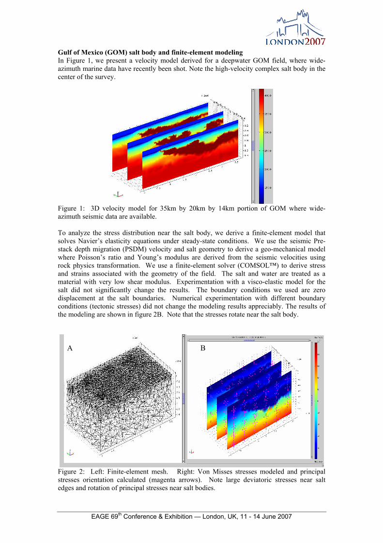
Gulf of Mexico (GOM) salt body and finite-element modeling In Figure 1, we present a velocity model derived for a deepwater GOM field, where wide-azimuth marine data have recently been shot. Note the high-velocity complex salt body in the center of the survey.

Figure 1: 3D velocity model for 35km by 20km by 14km portion of GOM where wide-azimuth seismic data are available. To analyze the stress distribution near the salt body, we derive a finite-element model that solves Navier’s elasticity equations under steady-state conditions. We use the seismic Pre-stack depth migration (PSDM) velocity and salt geometry to derive a geo-mechanical model where Poisson’s ratio and Young’s modulus are derived from the seismic velocities using rock physics transformation. We use a finite-element solver (COMSOL™) to derive stress and strains associated with the geometry of the field. The salt and water are treated as a material with very low shear modulus. Experimentation with a visco-elastic model for the salt did not significantly change the results. The boundary conditions we used are zero displacement at the salt boundaries. Numerical experimentation with different boundary conditions (tectonic stresses) did not change the modeling results appreciably. The results of the modeling are shown in figure 2B. Note that the stresses rotate near the salt body.

Figure 2: Left: Finite-element mesh. Right: Von Misses stresses modeled and principal stresses orientation calculated (magenta arrows). Note large deviatoric stresses near salt edges and rotation of principal stresses near salt bodies.

A B


Mapping stress to seismic anisotropy using TOE As seen in Figure 2b, the presence of the salt body generates large deviatoric stresses. Model results can be used to estimate the anisotropic material properties associated with the modeled stresses and strains. We use third-order elasticity (TOE) theory (Prioul et al., 2004) to derive the elastic anisotropic tensor using the background velocity model and the modeled strains. The relation between the background elastic stiffness 0

ijc is given in equation (1).

)(

)(),(

)(),(

)(),(

)(),(

22331551114404444

11331552214404455112215533144

06666

33221121112301323113311211123

01313

11221123312301212112211233111

01133

33111122211101122332211211111

01111

εεε

εεεεεε

εεεεεε

εεεεεε

εεεεεε

+++≅

+++≅+++≅

+++≅+++≅

+++≅+++≅

+++≅+++≅

cccc

cccccccc

cccccccc

cccccccc

cccccccc

(1)

We consider that the background elastic stiffness is considered to be isotropic and is related to the bulk and shear modulus (Mavko et al., 1998). To explore the range of anisotropy estimates we use TOE parameters from samples E1b and B1b listed in Prioul and Lebratt (2004) as GOM representative parameters. These values represent large and small stress sensitivity shale parameters. In Figure 3A we present the difference between the fast and slow velocity associated with TOE coefficients of high stress sensitivity (E1b). in the sub-volume we calculate velocity difference up to 300m/s. When we use low stress sensitivity TOE parameters (Figure 3B) we get anisotropy up to 25m/s difference between fast and slow velocity. Observation of seismic anisotropy in marine sediments In Figure 4, we present time gathers from three directions shot at azimuths 30, 90, and 330 degrees with respect to north. All gathers have been migrated with the isotropic velocity field using Kirchoff PSDM. The data have been mapped into time and we have picked five horizons along the different azimuths. Figure 4B shows 5 horizons picked on time sections (after NMO correction with a background velocity). We observe some anisotropy associated with different moveouts at different azimuths (Note that the flat events do not overlap in Figure 4B). In Figure 4C we plot all azimuth sorted by offsets. We can clearly observe the sinusoidal pattern small at near offsets and larger at far offsets. This behavior is consistent with elliptical velocity distribution as expected in the case of orthorhombic media. Note that all horizons are picked above the salt layer. We calculate the seismic anisotropy associated with the observed difference as follows: Using NMO equation we define the residual moveout for a given azimuth with respect to the velocity as 0

2220 /)( ττ −+=∆ rmsNMO VxT where 0τ is the zero offset twt and x is the offset.

Therefore, measuring residual travel time difference as a function of offset iNMOT )(∆δ for each azimuth can be related to the change in RMS velocity for the ith azimuth with respect to the reference velocity rmsV and can be calculating using the chain rule as:

( ) irms

rmsiNMO

iNMO VVxVxV

VTT δτδδ 3

221

2220 /)(

−+=

∂∆∂

=∆ (2)

where the difference between reference RMS velocity and the azimuthal velocity is rmsirmsi VVV _−=δ . Here we neglect differential NMO stretch. Given the 3 azimuths per horizons we can derive three velocities associated with the three azimuths. We now search for an elliptical velocity dependency that can be characterized using the relation


))(2cos(~_ irmsi azBAV −+ φ (Craft et al., 1996). We solve for BA, and φ using a non-linear minimization technique. The angle of orientation associated with the horizons is plotted in figure 5 together with the angle associated with the principal horizontal stresses. The RMS velocity anisotropy associated with the data is up to 30m/s in the rms data for horizon #4. This is consistent with TOE values higher slightly than sample B1b but lower that sample E1b.

Figure 3: Predicted difference between the fast and slow velocities predicted from TOE theory and finite-element modeling using salt geometry derived from the seismic image. A. Difference in 3D subset of 12km by 8km by 7km from the large 3D volume using TOE parameters E1b and predicting up to 300m/s difference in fast and slow velocities. B. Difference between fast and slow velocity using TOE parameters B1b predicting difference of only up to 25m/s between fast and slow velocity. Summary and conclusions In this paper, we show how stress distribution near salt bodies can cause large deviatoric stresses. The stresses modeled in this study are due to body loads only, and represent the different material properties and buoyancy effects associated with large salt bodies in the GOM. If we use TOE theory to model the sediment response to the stresses we show that we can expect velocity anisotropy. For the typical GOM parameters we used, we get ~ 300 m/s difference in interval velocity in the sedimentary layer above the salt. Time domain analysis of the wide-azimuth seismic response and angular traveltime analysis showed similar results. We note that we made many assumptions regarding the model and data analysis in this study; however, even in this example, we got reasonable results. This implies that using wide-azimuth seismic data provides information about the stress magnitude and directions.

Vpx- Vpy A B Vpx- Vpy


Figure 4: A. Three azimuths associated with the wide-azimuth marine survey. B. Five horizons picked on a migrated CIP time gather for three azimuths. Each azimuth is color-coded. Note that deeper horizons have more anisotropy. C. Horizons 3 and 4 show sinusoidal behavior consistent with elliptical velocity distribution.

Figure 5. A. Observed elliptical anisotropy in two of the picked Horizons. References Craft, K. L., Mallick, S., Meister, L. J., and Van Dok, R. [1997] Azimuthal anisotropy analysis from P-wave seismic traveltime data. 67th Meeting, Society of Exploration Geophysicists, Expanded Abstract, 1214-1217. Mavko, G., Dvorkin, J., and Mukerji, T. [1998] The rock physics handbook. Cambridge University Press. Prioul, R., and Lebrat, T. [2004] Calibration of velocity-stress relationships under hydrostatic stress for their use under non-hydrostatic stress conditions. 74th Meeting, Society of Exploration Geophysicists, Expanded Abstract, 1698-1701.

A B

-- 30 deg -- 90 deg -- 330 deg

. 30 deg

. 90 deg

. 330 deg

C

stress and seismic anisotropy near salt bodies – numerical...

Documents