streich, s. (2007). music complexity. a multi-faceted description of audio content. universitat...
TRANSCRIPT

7/29/2019 Streich, S. (2007). Music Complexity. a Multi-faceted Description of Audio Content. Universitat Pompeu Fabra.
http://slidepdf.com/reader/full/streich-s-2007-music-complexity-a-multi-faceted-description-of-audio 1/124
MUSIC COMPLEXITY: A MULTI-FACETED DESCRIPTION OF AUDIO CONTENT
A DISSERTATION SUBMITTED TO THE DEPARTMENT OF TECHNOLOGY OF THE
UNIVERSITAT POMPEU FABRA FOR THE PROGRAM IN COMPUTER SCIENCE AND DIGITAL
COMMUNICATION IN PARTIAL FULFILMENT OF THE REQUIREMENTS FOR THE DEGREE OF
–
DOCTOR PER LA UNIVERSITAT POMPEU FABRA
Sebastian Streich
2006

7/29/2019 Streich, S. (2007). Music Complexity. a Multi-faceted Description of Audio Content. Universitat Pompeu Fabra.
http://slidepdf.com/reader/full/streich-s-2007-music-complexity-a-multi-faceted-description-of-audio 2/124
Dipòsit legal: B.8926-2008
ISBN: 978-84-691-1752-1

7/29/2019 Streich, S. (2007). Music Complexity. a Multi-faceted Description of Audio Content. Universitat Pompeu Fabra.
http://slidepdf.com/reader/full/streich-s-2007-music-complexity-a-multi-faceted-description-of-audio 3/124
© Copyright by Sebastian Streich 2006
All Rights Reserved
ii

7/29/2019 Streich, S. (2007). Music Complexity. a Multi-faceted Description of Audio Content. Universitat Pompeu Fabra.
http://slidepdf.com/reader/full/streich-s-2007-music-complexity-a-multi-faceted-description-of-audio 4/124
DOCTORAL DISSERTATION DIRECTION
Dr. Xavier Serra
Department of Technology
Universitat Pompeu Fabra, Barcelona
This research was performed at the Music Technology Group of the Universitat Pompeu Fabra in Barcelona,
Spain. Primary support was provided by the EU projects FP6-507142 SIMAC http://www.semanticaudio.org.
iii

7/29/2019 Streich, S. (2007). Music Complexity. a Multi-faceted Description of Audio Content. Universitat Pompeu Fabra.
http://slidepdf.com/reader/full/streich-s-2007-music-complexity-a-multi-faceted-description-of-audio 5/124
iv

7/29/2019 Streich, S. (2007). Music Complexity. a Multi-faceted Description of Audio Content. Universitat Pompeu Fabra.
http://slidepdf.com/reader/full/streich-s-2007-music-complexity-a-multi-faceted-description-of-audio 6/124
Abstract
The complexity of music is one of the less intensively researched areas in music information retrieval so far.
Although very interesting findings have been reported over the years, there is a lack of a unified approach to
the matter. Relevant publications mostly concentrate on single aspects only and are scattered across differentdisciplines. Especially an automated estimation based on the audio material itself has hardly been addressed
in the past. However, it is not only an interesting and challenging topic, it also allows for very practical
applications.
The motivation for the presented research lies in the enhancement of human interaction with digital music
collections. As we will discuss, there is a variety of tasks to be considered, such as collection visualization,
play-list generation, or the automatic recommendation of music. While this thesis doesn’t deal with any
of these problems in deep detail it aims to provide a useful contribution to their solution in form of a set
of music complexity descriptors. The relevance of music complexity in this context will be emphasized by
an extensive review of studies and scientific publications from related disciplines, like music psychology,
musicology, information theory, or music information retrieval.
This thesis proposes a set of algorithms that can be used to compute estimates of music complexity
facets from musical audio signals. They focus on aspects of acoustics, rhythm, timbre, and tonality. Music
complexity is thereby considered on the coarse level of common agreement among human listeners. The
target is to obtain complexity judgements through automatic computation that resemble a naıve listener’s
point of view. Expert knowledge of specialists in particular musical domains is therefore out of the scope
of the proposed algorithms. While it is not claimed that this set of algorithms is complete or final, we will
see a selection of evaluations that gives evidence to the usefulness and relevance of the proposed methods
of computation. We will finally also take a look at possible future extensions and continuations for further
improvement, like the consideration of complexity on the level of musical structure.
v

7/29/2019 Streich, S. (2007). Music Complexity. a Multi-faceted Description of Audio Content. Universitat Pompeu Fabra.
http://slidepdf.com/reader/full/streich-s-2007-music-complexity-a-multi-faceted-description-of-audio 7/124
vi
7/29/2019 Streich, S. (2007). Music Complexity. a Multi-faceted Description of Audio Content. Universitat Pompeu Fabra.
http://slidepdf.com/reader/full/streich-s-2007-music-complexity-a-multi-faceted-description-of-audio 8/124
Acknowledgments
During my work on this thesis I learned many things and that is not only in the professional, but also in the
personal sense. During my stay at the Music Technology Group I had the luck to experience a unique climate
of encouragement, support, and open communication that was essential for being able to proceed so fast andsmoothly with my research activities. It goes without saying that such a climate doesn’t come by itself, but
is due to every individual’s effort to create and maintain this fruitful environment. I therefore want to express
my gratitude to the whole MTG as the great team it has been for me during my time in Barcelona.
In particular and at the first place I would like to thank Dr. Xavier Serra, my supervisor, for giving me
the opportunity to work on this very interesting topic as a member of the MTG. Also, and specially, I want to
thank Perfecto Herrera for providing countless suggestions and constant support for my work in this research
project. Without him I certainly would not be at this point now.
Further thanks go to my colleagues from Office 316, Bee Suan Ong, Emilia Gomez, and Enric Guaus
for many fruitful discussions and important feedback. I also want to thank all the other people – directly or
indirectly – involved in the success of the SIMAC research project for their appreciated cooperation.This research was funded by a scholarship from Universitat Pompeu Fabra and by the EU-FP6-IST-
507142 project SIMAC. I am thankful for this support, which was a crucial economic basis for my research.
On the personal side I also want to thank my wife and my family, who provided me with the support,
encouragement, and sometimes also with the necessary distraction that helped me to keep going.
Finally, a special thank you note has to be included for my “sister in law” for helping out with the printing
and everything else. I owe you a coffee. ;-)
Hamamatsu, Japan Sebastian Streich
November 16, 2006
vii

7/29/2019 Streich, S. (2007). Music Complexity. a Multi-faceted Description of Audio Content. Universitat Pompeu Fabra.
http://slidepdf.com/reader/full/streich-s-2007-music-complexity-a-multi-faceted-description-of-audio 9/124
viii

7/29/2019 Streich, S. (2007). Music Complexity. a Multi-faceted Description of Audio Content. Universitat Pompeu Fabra.
http://slidepdf.com/reader/full/streich-s-2007-music-complexity-a-multi-faceted-description-of-audio 10/124
List of Figures
1.1 Illustration of three different views on digital music. . . . . . . . . . . . . . . . . . . . . . . 3
1.2 Screenshot from a music browser interface displaying part of a song collection organized by
danceability and dynamic complexity. . . . . . . . . . . . . . . . . . . . . . . . . . . . . . 5
1.3 The Wundt curve for the relation between music complexity and preference. . . . . . . . . . 9
2.1 Complete order, chaos, and complete disorder [from Edmonds (1995)]. . . . . . . . . . . . . 15
2.2 Possible inclusions [from Edmonds (1995)]. . . . . . . . . . . . . . . . . . . . . . . . . . . 16
2.3 Example for model selection with Minimum Description Length [from Grunwald (2005)]. . 23
3.1 Illustration of the Implication-Realization Process [from Schellenberg et al. (2002)]. . . . . . 30
3.2 Tree obtained with algorithmic clustering of 12 piano pieces [from Cilibrasi et al. (2004)]. . 36
3.3 Plots from Voss and Clarke (1975). Left: log10(loudness fluctuation) against log10(f ) for a)
Scott Joplin piano rags, b) Classical radio station, c) Rock station, d) News and talk station;
Right: log10(pitch fluctuation) against log10(f ) for a) Classical radio station, b) Jazz and
Blues station, c) Rock station, d) News and talk station. . . . . . . . . . . . . . . . . . . . . 41
3.4 Average DFA exponent α for different music genres [from Jennings et al. (2004)] . . . . . . 43
4.1 Instantaneous loudness as in eq. 4.3 (dots), global loudness as in eq. 4.4 (grey solid line), and
average distance margin as in eq. 4.5 (dashed lines) for four example tracks. . . . . . . . . . 49
4.2 Frequency weighting curves for the outer ear. . . . . . . . . . . . . . . . . . . . . . . . . . 51
4.3 Instantaneous total loudness values (eq. 4.17) on logarithmic scale for the same four tracks
shown in figure 4.1. . . . . . . . . . . . . . . . . . . . . . . . . . . . . . . . . . . . . . . . 54
4.4 Snapshots of energy distributions on 180°horizontal plane for two example tracks (track1=
modern electronic music, track2= historic jazz recording). . . . . . . . . . . . . . . . . . . 57
4.5 Schema for timbre complexity estimation with unsupervised HMM training . . . . . . . . . 60
4.6 Timbre symbol sequences for excerpts of a) Baroque cembalo music, b) a modern Musical
song with orchestra. . . . . . . . . . . . . . . . . . . . . . . . . . . . . . . . . . . . . . . . 63
4.7 Block diagram of timbral complexity computation based on spectral envelope matching. . . 65
ix
7/29/2019 Streich, S. (2007). Music Complexity. a Multi-faceted Description of Audio Content. Universitat Pompeu Fabra.
http://slidepdf.com/reader/full/streich-s-2007-music-complexity-a-multi-faceted-description-of-audio 11/124
4.8 Band loudness similarities (eq. 4.28) for three music excerpts: a) bagpipe ensemble, b) clas-
sical symphony, c) rap (the thick line at the bottom marks the sections that are identified as
voice content and therefore left out in the complexity computation). The timbral complexity
is calculated as the percentage of frames where the similarity is equal to zero. . . . . . . . . 66
4.9 Distance measures for tonal complexity computation: a) inverted correlation D[i]1 , b) city
block distance D[i]2 , c) linear combination, d) corresponding HPCP data (before moving av-
erage). . . . . . . . . . . . . . . . . . . . . . . . . . . . . . . . . . . . . . . . . . . . . . 70
4.10 Excerpts from the time series s(n) for three example pieces from different musical genres. . 72
4.11 Double logarithmic plots of mean residual over time scales. . . . . . . . . . . . . . . . . . . 73
4.12 DFA exponent functions for the three example tracks from figure 4.10. . . . . . . . . . . . . 74
5.1 Screenshot from the second part of the websurvey. . . . . . . . . . . . . . . . . . . . . . . . 80
5.2 Average percentage of correct predictions with subject models for the binary complexity (top)
and liking ratings (bottom) according to different demographic groups. . . . . . . . . . . . . 86
5.3 Top-eight labels with the highest number of assigned artists. . . . . . . . . . . . . . . . . . 88
5.4 α-levels for 60 techno (o) and 60 film score tracks (x), unordered. . . . . . . . . . . . . . . 89
5.5 Distributions on deciles for the twelve labels with most significant deviation from equal dis-
tribution (solid horizontal lines). . . . . . . . . . . . . . . . . . . . . . . . . . . . . . . . . 90
x

7/29/2019 Streich, S. (2007). Music Complexity. a Multi-faceted Description of Audio Content. Universitat Pompeu Fabra.
http://slidepdf.com/reader/full/streich-s-2007-music-complexity-a-multi-faceted-description-of-audio 12/124
List of Tables
2.1 Approximate number of page hits found by the Google search engine for different search
phrases. . . . . . . . . . . . . . . . . . . . . . . . . . . . . . . . . . . . . . . . . . . . . . 14
3.1 Features used by Scheirer et al. (2000) in their experiment. . . . . . . . . . . . . . . . . . . 39
5.1 Statistics about the subjects who answered the web survey. . . . . . . . . . . . . . . . . . . 82
5.2 Pearson correlation for the complexity descriptors with averaged ratings of complexity and
liking (significance at p < 0.01 is indicated by italics). . . . . . . . . . . . . . . . . . . . . 84
5.3 The ten most significantly deviating labels in each direction. . . . . . . . . . . . . . . . . . 89
5.4 Confusion matrix of three class machine learning experiment. . . . . . . . . . . . . . . . . 92
5.5 Feature combinations used in the trackball experiments. . . . . . . . . . . . . . . . . . . . . 93
5.6 Mean, standard deviation, and significance margin for the search time in seconds of each
setup [Andric et al. (2006)]. . . . . . . . . . . . . . . . . . . . . . . . . . . . . . . . . . . . 94
xi

7/29/2019 Streich, S. (2007). Music Complexity. a Multi-faceted Description of Audio Content. Universitat Pompeu Fabra.
http://slidepdf.com/reader/full/streich-s-2007-music-complexity-a-multi-faceted-description-of-audio 13/124
xii

7/29/2019 Streich, S. (2007). Music Complexity. a Multi-faceted Description of Audio Content. Universitat Pompeu Fabra.
http://slidepdf.com/reader/full/streich-s-2007-music-complexity-a-multi-faceted-description-of-audio 14/124
Contents
Abstract v
Acknowledgments vii
1 Introduction 1
1.1 Research Context and Motivation . . . . . . . . . . . . . . . . . . . . . . . . . . . . . . . . 1
1.1.1 Music Tracks as Data Files . . . . . . . . . . . . . . . . . . . . . . . . . . . . . . . 1
1.1.2 Problems with Digital Collections . . . . . . . . . . . . . . . . . . . . . . . . . . . 2
1.1.3 Semantic Descriptors as a Perspective . . . . . . . . . . . . . . . . . . . . . . . . . 4
1.2 Thesis Goals . . . . . . . . . . . . . . . . . . . . . . . . . . . . . . . . . . . . . . . . . . . 6
1.3 Applicability of Music Complexity . . . . . . . . . . . . . . . . . . . . . . . . . . . . . . . 8
1.3.1 Enhanced Visualization and Browsing . . . . . . . . . . . . . . . . . . . . . . . . . 9
1.3.2 Playlist Generation . . . . . . . . . . . . . . . . . . . . . . . . . . . . . . . . . . . 10
1.3.3 Song Retrieval . . . . . . . . . . . . . . . . . . . . . . . . . . . . . . . . . . . . . 11
1.4 Thesis Outline . . . . . . . . . . . . . . . . . . . . . . . . . . . . . . . . . . . . . . . . . . 11
2 The Meaning of Complexity 13
2.1 The Informal View . . . . . . . . . . . . . . . . . . . . . . . . . . . . . . . . . . . . . . . 13
2.1.1 Difficult Description and Felt Rules . . . . . . . . . . . . . . . . . . . . . . . . . . 13
2.1.2 Subjectivity . . . . . . . . . . . . . . . . . . . . . . . . . . . . . . . . . . . . . . . 16
2.1.3 Trendy Buzzword? . . . . . . . . . . . . . . . . . . . . . . . . . . . . . . . . . . . 18
2.2 The Formal View . . . . . . . . . . . . . . . . . . . . . . . . . . . . . . . . . . . . . . . . 19
2.2.1 Information and Entropy . . . . . . . . . . . . . . . . . . . . . . . . . . . . . . . . 20
2.2.2 Kolmogorov Complexity . . . . . . . . . . . . . . . . . . . . . . . . . . . . . . . . 21
2.2.3 Stochastic Complexity . . . . . . . . . . . . . . . . . . . . . . . . . . . . . . . . . 22
2.3 Implications for our goals . . . . . . . . . . . . . . . . . . . . . . . . . . . . . . . . . . . . 23
3 Former Work on the Complexity of Music 25
3.1 The Preferred Level of Complexity . . . . . . . . . . . . . . . . . . . . . . . . . . . . . . . 25
xiii

7/29/2019 Streich, S. (2007). Music Complexity. a Multi-faceted Description of Audio Content. Universitat Pompeu Fabra.
http://slidepdf.com/reader/full/streich-s-2007-music-complexity-a-multi-faceted-description-of-audio 15/124
3.1.1 Complexity and Aesthetics . . . . . . . . . . . . . . . . . . . . . . . . . . . . . . . 25
3.1.2 Psychological Experiments . . . . . . . . . . . . . . . . . . . . . . . . . . . . . . . 26
3.1.3 Musicological Studies . . . . . . . . . . . . . . . . . . . . . . . . . . . . . . . . . 28
3.1.4 Conclusion . . . . . . . . . . . . . . . . . . . . . . . . . . . . . . . . . . . . . . . 29
3.2 Computing Complexity on Symbolic Representations . . . . . . . . . . . . . . . . . . . . . 29
3.2.1 Models for Melodic Complexity . . . . . . . . . . . . . . . . . . . . . . . . . . . . 29
3.2.2 Models for Rhythmic Complexity . . . . . . . . . . . . . . . . . . . . . . . . . . . 32
3.2.3 Models for Harmonic Complexity . . . . . . . . . . . . . . . . . . . . . . . . . . . 33
3.2.4 Pressing’s Music Complexity . . . . . . . . . . . . . . . . . . . . . . . . . . . . . 34
3.2.5 Algorithmic Clustering . . . . . . . . . . . . . . . . . . . . . . . . . . . . . . . . . 35
3.2.6 Conclusion . . . . . . . . . . . . . . . . . . . . . . . . . . . . . . . . . . . . . . . 37
3.3 Computing Complexity on Audio Signals . . . . . . . . . . . . . . . . . . . . . . . . . . . 373.3.1 Complexity of Short Musical Excerpts . . . . . . . . . . . . . . . . . . . . . . . . . 38
3.3.2 Power Laws . . . . . . . . . . . . . . . . . . . . . . . . . . . . . . . . . . . . . . . 39
3.3.3 Detrended Fluctuation Analysis . . . . . . . . . . . . . . . . . . . . . . . . . . . . 42
3.3.4 Conclusion . . . . . . . . . . . . . . . . . . . . . . . . . . . . . . . . . . . . . . . 43
4 Complexity Facets and their Implementation 45
4.1 Working on Facets . . . . . . . . . . . . . . . . . . . . . . . . . . . . . . . . . . . . . . . 45
4.2 Acoustic Complexities . . . . . . . . . . . . . . . . . . . . . . . . . . . . . . . . . . . . . 46
4.2.1 Implementation of the Dynamic Component . . . . . . . . . . . . . . . . . . . . . . 47
4.2.2 Implementation of the Spatial Component . . . . . . . . . . . . . . . . . . . . . . . 53
4.3 Timbral Complexity . . . . . . . . . . . . . . . . . . . . . . . . . . . . . . . . . . . . . . . 58
4.3.1 Implementations of Timbre Complexity . . . . . . . . . . . . . . . . . . . . . . . . 58
4.4 Tonal Complexity . . . . . . . . . . . . . . . . . . . . . . . . . . . . . . . . . . . . . . . . 67
4.4.1 Implementations of Tonal Complexity . . . . . . . . . . . . . . . . . . . . . . . . . 67
4.5 Rhythmic Complexity . . . . . . . . . . . . . . . . . . . . . . . . . . . . . . . . . . . . . . 71
4.5.1 Implementation of Danceability . . . . . . . . . . . . . . . . . . . . . . . . . . . . 71
5 Evaluation 77
5.1 Methods of Evaluation . . . . . . . . . . . . . . . . . . . . . . . . . . . . . . . . . . . . . 77
5.2 Evaluation with Human Ratings . . . . . . . . . . . . . . . . . . . . . . . . . . . . . . . . 79
5.2.1 Survey Design, Material, and Subjects . . . . . . . . . . . . . . . . . . . . . . . . . 79
5.2.2 The Obtained Data . . . . . . . . . . . . . . . . . . . . . . . . . . . . . . . . . . . 82
5.2.3 Results of the Analysis . . . . . . . . . . . . . . . . . . . . . . . . . . . . . . . . . 83
5.3 Evaluation with Existing Labels . . . . . . . . . . . . . . . . . . . . . . . . . . . . . . . . 87
5.3.1 The Dataset . . . . . . . . . . . . . . . . . . . . . . . . . . . . . . . . . . . . . . . 87
5.3.2 Results . . . . . . . . . . . . . . . . . . . . . . . . . . . . . . . . . . . . . . . . . 87
xiv

7/29/2019 Streich, S. (2007). Music Complexity. a Multi-faceted Description of Audio Content. Universitat Pompeu Fabra.
http://slidepdf.com/reader/full/streich-s-2007-music-complexity-a-multi-faceted-description-of-audio 16/124
5.3.3 Concluding Remarks . . . . . . . . . . . . . . . . . . . . . . . . . . . . . . . . . . 92
5.4 Evaluation through Simulated Searching . . . . . . . . . . . . . . . . . . . . . . . . . . . . 92
5.4.1 Experimental Setup . . . . . . . . . . . . . . . . . . . . . . . . . . . . . . . . . . . 92
5.4.2 Results . . . . . . . . . . . . . . . . . . . . . . . . . . . . . . . . . . . . . . . . . 93
5.5 Conclusion . . . . . . . . . . . . . . . . . . . . . . . . . . . . . . . . . . . . . . . . . . . 94
6 Conclusions and Future Work 95
6.1 Summary of the Achievements . . . . . . . . . . . . . . . . . . . . . . . . . . . . . . . . . 96
6.2 Open issues . . . . . . . . . . . . . . . . . . . . . . . . . . . . . . . . . . . . . . . . . . . 97
6.2.1 Structural Complexity . . . . . . . . . . . . . . . . . . . . . . . . . . . . . . . . . 97
6.2.2 Other Facets to be considered . . . . . . . . . . . . . . . . . . . . . . . . . . . . . 97
6.2.3 Application-oriented Evaluation . . . . . . . . . . . . . . . . . . . . . . . . . . . . 98
6.3 Music Complexity in the Future of Music Content Processing . . . . . . . . . . . . . . . . . 98
Bibliography 99
xv

7/29/2019 Streich, S. (2007). Music Complexity. a Multi-faceted Description of Audio Content. Universitat Pompeu Fabra.
http://slidepdf.com/reader/full/streich-s-2007-music-complexity-a-multi-faceted-description-of-audio 17/124
xvi

7/29/2019 Streich, S. (2007). Music Complexity. a Multi-faceted Description of Audio Content. Universitat Pompeu Fabra.
http://slidepdf.com/reader/full/streich-s-2007-music-complexity-a-multi-faceted-description-of-audio 18/124
Chapter 1
Introduction
1.1 Research Context and Motivation
Music, in the western cultural world at least, is present in everybody’s life. It can be found not only at its
“traditional” places like opera houses or discotheques, but appears in kitchens and nurseries, in cars and
airports, bars and restaurants, parks and sport centers and in many other places. With the increased mobility
of music reproduction devices nowadays everybody can bring his own personal music along and listen to it
almost anywhere. But this enhanced availability of music also means that concentrated and active listening
has become rare. Often music serves as a background while the listener is doing something else, it is used
as an acoustical “gap filler”, or as an emotional trigger [see North and Hargreaves (1997c)]. New ways of
dissemination for music have been arising and never before it has been as easy as today to get access to such
a huge amount of music (more than a million titles are available from a single music portal) without even
having to get up from one’s chair. Yet, it is not always easy to find what one is looking for.
1.1.1 Music Tracks as Data Files
With a broader public becoming aware of efficient audio coding techniques during the last decade, the amount
of music being stored and collected in digital formats increased rapidly. While in former times a music
collection consisted of a conglomeration of physical media in form of vinyl discs, analogue or digital tapes,
and later also compact discs, a new kind of collections emerged due to the new formats. No longer is the
music in these collections attached to a physical medium, but exists merely as a string of bits that can, very
easily and without degradation in quality, be moved and copied from any digital storing device to any other
one. This property, apart from being very convenient, again reinforced the rapid spread of the new formats,
by making it as easy as never before to share and exchange music with virtually anybody on the planet (or at
least with the roughly 16% of our world’s population who have access to the interne t1).
1according to http://www.internetworldstats.com/stats.htm
1

7/29/2019 Streich, S. (2007). Music Complexity. a Multi-faceted Description of Audio Content. Universitat Pompeu Fabra.
http://slidepdf.com/reader/full/streich-s-2007-music-complexity-a-multi-faceted-description-of-audio 19/124
2 CHAPTER 1. INTRODUCTION
Nowadays, the music industry managed to hinder the wild exchange of music by filing lawsuits against
operators and private users of such content exchange networks. But digital music collections already exist in
large numbers and the concept of storing music tracks as digital files with all its advantages is an established
fact for many music consumers. Lately, legal options to buy digital music online and receive it by file transfer
over the World Wide Web are arising, often combined with some sort of digital rights management that is
supposed to prevent consumers from “shamelessly” copying and sharing their new acquisitions. Last but not
least, alternative models of copyrighting and licensing musical content are emerging (e. g. creative commons2)
and contribute a small but growing part to the music that can be found and obtained from the internet. David
Kusek and Gerd Leonhard, two music futurists, even coin the term of “music as water” [ Kusek and Leonhard
(2005)] in order to describe the change of attitude towards music, music consumption, and music ownership
that is in the process of establishing itself:
“Imagine a world where music flows all around us, like water, or like electricity, and where
access to music becomes a kind of ‘utility’. Not for free, per se, but certainly for what feels like
free.”
While this situation still remains only an imagination nowadays, there are already plenty of examples
of developing communities of people who share their own digital creations on a very large scale (although
many of those creations might be in fact remixes of others’ material and thus again problematic in terms of
traditional copyright laws). Two outstanding examples here are Flickr3 for digital photos and images, and
YouTube4 for digital video clips each with millions of users. An example from the music domain is the
Freesound project 5 where audio samples of all types of sounds are shared for the use in new digital creations.
1.1.2 Problems with Digital Collections
Despite the many advantages that came with this “digital revolution” we can observe some negative effects,
too. The flexibility that music tracks, in form of individual files, provide goes along with a demand for
a proper storage organization and labelling or tagging. While in a physical collection an item might be
declared lost when it cannot be found, in a large virtual collection this can be said already when there are no
means to search for it. This is especially true for shared and foreign collections like commercial online music
shops and community portals. Even if tags are made available by the provider they cannot be guaranteed to
be complete and consistent.
The freedom to create personalized play lists and to listen to music tracks independently from concepts
like albums or compilations requires on the other hand a good knowledge of the collection at hand in order
to arrive at satisfying results. Navigation and utilization become difficult and limited, when typing errors in
2http://creativecommons.org/ 3http://www.flickr.com4http://www.youtube.com5http://freesound.iua.upf.edu/

7/29/2019 Streich, S. (2007). Music Complexity. a Multi-faceted Description of Audio Content. Universitat Pompeu Fabra.
http://slidepdf.com/reader/full/streich-s-2007-music-complexity-a-multi-faceted-description-of-audio 20/124
1.1. RESEARCH CONTEXT AND MOTIVATION 3
Figure 1.1: Illustration of three different views on digital music.
filenames, an insufficient taxonomy for file organization, and inconsistency in the manually assigned labels
occur in such a collection.
Figure 1.1 shows three simplified views on a digital music collection that illustrate the situation. In
the center we have the traditional interface perspective, where each track is identified by a name that was
assigned to it and is placed somewhere inside a folder tree, where folders might be arranged according
to albums, artists, genres, or any other concept of organization. On the left we have a view of a human
user interacting with the collection. For him the items are associated with semantic connotations. A song
in the collection has a recognizable musical theme, belongs to a certain style, evokes a particular mood,
features certain instruments, etc. However, if he did not put all this information into the system by choosing
a sophisticated folder structure or by excessive manual tagging, these connotations are simply not available
for his interaction. Finally, on the right side we see how different the perspective of the machine is. For the
computer the file names are only pointers to strings of binary symbols on a storage medium. The type of
“connotations” we find here are only of the technical type including things like the bit rate, the file size, or the
sampling frequency. Another aspect of bit strings representing music is their volatility and reproducibility.
With the move of a finger they can be erased and they are gone without leaving any trace. Or they can be
replicated with very little effort basically infinite times at no cost other than the disk space to store them.
Especially the latter has an impact on the value that is assigned to such an item. According to the theory of
supply and demand a commodity with finite demand but infinite supply has a price of zero (of course thiscannot be applied directly to music). As an illustration: If I go into a record shop to buy an album and the
salesman gives me two copies for the price of one, I will consider this a true benefit, because I can give one
copy to a friend or resell it. If I buy the same album from an online shop and they offer me to download it
twice by paying only once, I would just find it silly. This gives a good hint for understanding why people are
so “generous” to offer their complete collection of music files for anybody to download without any charge.
And it also helps understanding why people do not feel shy to download or copy music from others without
7/29/2019 Streich, S. (2007). Music Complexity. a Multi-faceted Description of Audio Content. Universitat Pompeu Fabra.
http://slidepdf.com/reader/full/streich-s-2007-music-complexity-a-multi-faceted-description-of-audio 21/124
4 CHAPTER 1. INTRODUCTION
paying and without feeling they do something unjust. Especially in the times of free peer-to-peer music
sharing networks this configuration boosted the dissemination and the enforcement of digital music formats,
which are a matter of fact nowadays. On the other hand, this excess of digital tracks may have decreased the
appreciation for the individual item. So some private collections have been extended for the sake of collecting
rather than because of a particular interest in the material.
Summarizing we can say that today probably many hard disks exist which contain a large collection of
digital music, but the owner is ignorant about the full potential of it. Even if he or she is not, it means a lot of
effort to fully exploit it and rather sooner than later the currently available tools reach their limits. With the
new way of music dissemination through online portals like for example iTunes6 or Y!music7 the problem
of searching, browsing, and navigating a (unfamiliar) music collection is brought to an even larger scale and
begs for new solutions.
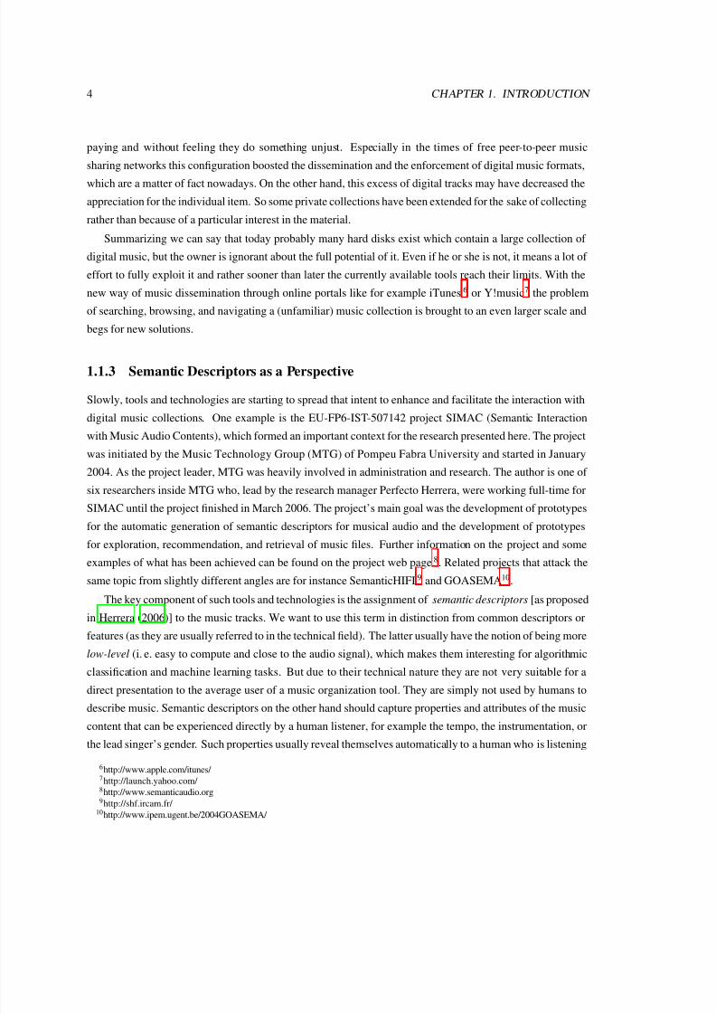
1.1.3 Semantic Descriptors as a Perspective
Slowly, tools and technologies are starting to spread that intent to enhance and facilitate the interaction with
digital music collections. One example is the EU-FP6-IST-507142 project SIMAC (Semantic Interaction
with Music Audio Contents), which formed an important context for the research presented here. The project
was initiated by the Music Technology Group (MTG) of Pompeu Fabra University and started in January
2004. As the project leader, MTG was heavily involved in administration and research. The author is one of
six researchers inside MTG who, lead by the research manager Perfecto Herrera, were working full-time for
SIMAC until the project finished in March 2006. The project’s main goal was the development of prototypes
for the automatic generation of semantic descriptors for musical audio and the development of prototypes
for exploration, recommendation, and retrieval of music files. Further information on the project and some
examples of what has been achieved can be found on the project web page 8. Related projects that attack the
same topic from slightly different angles are for instance SemanticHIFI9 and GOASEMA10.
The key component of such tools and technologies is the assignment of semantic descriptors [as proposed
in Herrera (2006)] to the music tracks. We want to use this term in distinction from common descriptors or
features (as they are usually referred to in the technical field). The latter usually have the notion of being more
low-level (i. e. easy to compute and close to the audio signal), which makes them interesting for algorithmic
classification and machine learning tasks. But due to their technical nature they are not very suitable for a
direct presentation to the average user of a music organization tool. They are simply not used by humans to
describe music. Semantic descriptors on the other hand should capture properties and attributes of the musiccontent that can be experienced directly by a human listener, for example the tempo, the instrumentation, or
the lead singer’s gender. Such properties usually reveal themselves automatically to a human who is listening
6http://www.apple.com/itunes/ 7http://launch.yahoo.com/ 8http://www.semanticaudio.org9http://shf.ircam.fr/
10http://www.ipem.ugent.be/2004GOASEMA/

7/29/2019 Streich, S. (2007). Music Complexity. a Multi-faceted Description of Audio Content. Universitat Pompeu Fabra.
http://slidepdf.com/reader/full/streich-s-2007-music-complexity-a-multi-faceted-description-of-audio 22/124
1.1. RESEARCH CONTEXT AND MOTIVATION 5
Figure 1.2: Screenshot from a music browser interface displaying part of a song collection organized by
danceability and dynamic complexity.
to a music track and hence are potentially very relevant information when selecting and organizing music in
a collection. Therefore a link between the pure digital audio data and the semantic concepts describing the
content offers much more natural ways of searching in music collections than it is currently possible. Instead
of being limited to titles, artists, and genres as the means of a query even very subtle or abstract aspects of
music could be used provided the semantic descriptors are assigned to the tracks. A common way to put it
is by saying that with these descriptors we try to close the semantic gap [see e. g. Celma (2006)]. Some of
the semantic connotations of the left side from figure 1.1 become available for interacting with the collection.
Apart from the enhanced querying, there are also other possibilities arising. Browsing through a collection,
be it one’s own or a foreign one, where different musical aspects are visualized (see figure 1.2) is not only
amusing, but it may also lead to a better understanding of the music. Similarities between different styles
or artists can be discovered, the evolution of a band along time can be tracked, extreme examples can be
identified. This playful and educational side effect could then again lead to a more attentive way of music
listening, increasing pleasure and appreciation.
But the availability of such descriptors does not only bring additional opportunities for humans interacting
with music. Organized in a machine readable way, this meta-data forms an access point for information
processing devices to the properties of music which are relevant for a human listener. Basically, this allows
computers to mimic a human’s music perception behavior and establishes a direct connection between the

7/29/2019 Streich, S. (2007). Music Complexity. a Multi-faceted Description of Audio Content. Universitat Pompeu Fabra.
http://slidepdf.com/reader/full/streich-s-2007-music-complexity-a-multi-faceted-description-of-audio 23/124
6 CHAPTER 1. INTRODUCTION
left and the right of figure 1.1. Instead of the human browsing the collection, the computer could do this
automatically and identify for example clusters of similar tracks. Thus, the computer is enabled to generate
play lists according to given criteria or to recommend to the user similar tracks to a selected example track.
So we see that providing machine readable semantic descriptors for the tracks in a collection opens the
door for a large variety of interesting methods of sorting, searching, filtering, clustering, classifying, and
visualizing. But how can we arrive there? Different ways exist to assign semantic descriptors to music. It
is possible (although expensive) to have a group of music professionals annotate them. Some web-based
music recommendation services follow this strategy (e. g. Pandora11). This first option is of course usually
not feasible in the case of private collections. Still, the meta-data - once annotated - could be stored in a public
database and would then be associated through a fingerprinting service with the files in a private collection.
To some extent the descriptors can also be assigned by a whole community of listeners by majority vote or
by using collaborative filtering techniques. This second option involves quite some coordinative efforts and
furthermore causes a delay until reliable data for a new track becomes available. Really new material will
come without tags and will take its time until it has been discovered and labelled by a sufficient number of
people. The third, most practical and versatile option however is the automatic computation of descriptors
based on the audio file itself. This way, an objective, consistent, inexpensive, and detailed annotation can be
accomplished. The research presented here is about this third option of descriptor extraction.
1.2 Thesis Goals
This thesis proposes to consider a specific type of semantic descriptors in the context of music information
retrieval applications. We want to coin the term music complexity descriptors for them. It is a truism that
music can only be experienced as a temporal process. Therefore, when providing a description of music it is
necessary to capture aspects of its temporal evolution and organization in addition to global descriptors, that
only consider simple statistics like the maximum, mean or variance of instantaneous properties of an entire
music track.
The algorithms proposed in this thesis focus on the automated computation of music complexity as it is
perceived12 by human listeners. We regard the complexity of music as a high-level, intuitive attribute, which
can be experienced directly or indirectly by the active listener, so it could be estimated by empirical methods.
In particular we define the complexity as that property of a musical unit that determines how much effort the
listener has to put into following and understanding it (see chapter 2 for a more detailed discussion of the
term complexity).
The proposed algorithms are intended to provide a compact description of music as a temporal process.
The intended use should be seen in facilitating user interaction with music databases including collection
visualization, browsing, searching, and automatic recommendation. Since music has different and partly
11http://www.pandora.com12Throughout this document we will use the term “perception” although “cognition” might be considered more appropriate at some
places. However, we want to omit this distinction here and consecutively use “perceptual” as the contrasting term to “technical”.
7/29/2019 Streich, S. (2007). Music Complexity. a Multi-faceted Description of Audio Content. Universitat Pompeu Fabra.
http://slidepdf.com/reader/full/streich-s-2007-music-complexity-a-multi-faceted-description-of-audio 24/124
1.2. THESIS GOALS 7
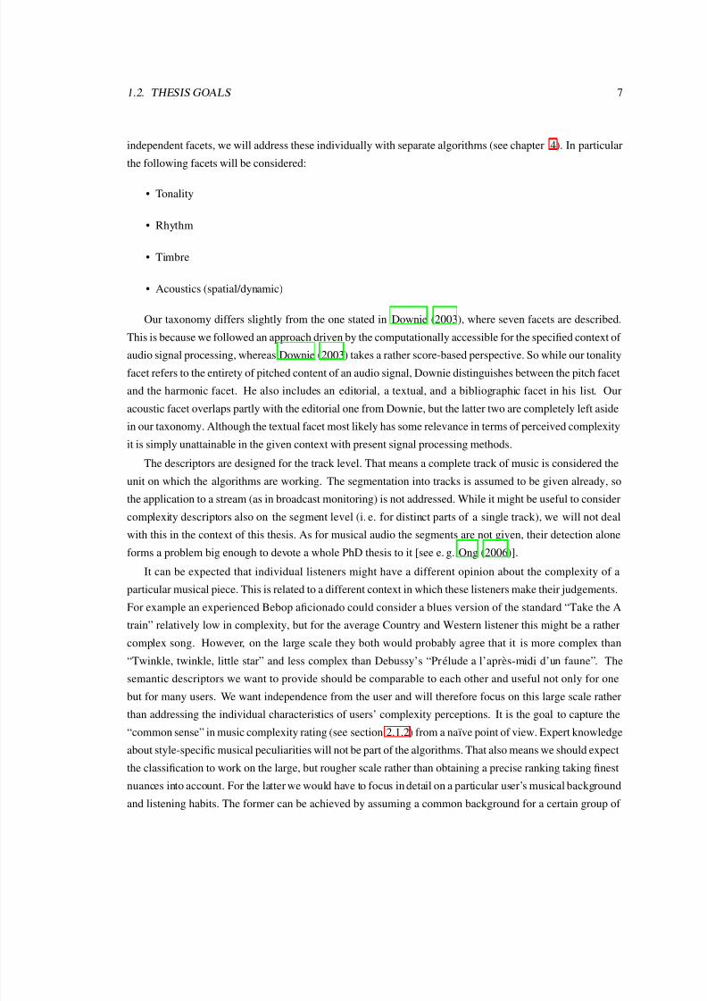
independent facets, we will address these individually with separate algorithms (see chapter 4). In particular
the following facets will be considered:
• Tonality
• Rhythm
• Timbre
• Acoustics (spatial/dynamic)
Our taxonomy differs slightly from the one stated in Downie (2003), where seven facets are described.
This is because we followed an approach driven by the computationally accessible for the specified context of
audio signal processing, whereas Downie (2003) takes a rather score-based perspective. So while our tonality
facet refers to the entirety of pitched content of an audio signal, Downie distinguishes between the pitch facet
and the harmonic facet. He also includes an editorial, a textual, and a bibliographic facet in his list. Our
acoustic facet overlaps partly with the editorial one from Downie, but the latter two are completely left aside
in our taxonomy. Although the textual facet most likely has some relevance in terms of perceived complexity
it is simply unattainable in the given context with present signal processing methods.
The descriptors are designed for the track level. That means a complete track of music is considered the
unit on which the algorithms are working. The segmentation into tracks is assumed to be given already, so
the application to a stream (as in broadcast monitoring) is not addressed. While it might be useful to consider
complexity descriptors also on the segment level (i. e. for distinct parts of a single track), we will not deal
with this in the context of this thesis. As for musical audio the segments are not given, their detection alone
forms a problem big enough to devote a whole PhD thesis to it [see e. g. Ong (2006)].
It can be expected that individual listeners might have a different opinion about the complexity of a
particular musical piece. This is related to a different context in which these listeners make their judgements.
For example an experienced Bebop aficionado could consider a blues version of the standard “Take the A
train” relatively low in complexity, but for the average Country and Western listener this might be a rather
complex song. However, on the large scale they both would probably agree that it is more complex than
“Twinkle, twinkle, little star” and less complex than Debussy’s “Prelude a l’apres-midi d’un faune”. The
semantic descriptors we want to provide should be comparable to each other and useful not only for one
but for many users. We want independence from the user and will therefore focus on this large scale ratherthan addressing the individual characteristics of users’ complexity perceptions. It is the goal to capture the
“common sense” in music complexity rating (see section 2.1.2) from a naıve point of view. Expert knowledge
about style-specific musical peculiarities will not be part of the algorithms. That also means we should expect
the classification to work on the large, but rougher scale rather than obtaining a precise ranking taking finest
nuances into account. For the latter we would have to focus in detail on a particular user’s musical background
and listening habits. The former can be achieved by assuming a common background for a certain group of

7/29/2019 Streich, S. (2007). Music Complexity. a Multi-faceted Description of Audio Content. Universitat Pompeu Fabra.
http://slidepdf.com/reader/full/streich-s-2007-music-complexity-a-multi-faceted-description-of-audio 25/124
8 CHAPTER 1. INTRODUCTION
users and then restricting the validity of the provided models only to this group. We chose the group of non-
expert music listeners with western cultural background as the intended users of the developed descriptors,
since it forms a large fraction of the users dealing with the above mentioned music databases.
Finally it has to be said that the proposed algorithms only form a starting point to enter the domain of
music complexity related descriptors. Already the list of facets that were tackled during the research reported
here cannot be called complete. For example the complexity of the lyrics is a certainly relevant descriptor
that has not been addressed at all, since the focus was on algorithms that operate exclusively on the audio
data. Other examples would be the musical structure and the melody. We will talk about possibilities for
future research in section 6.2 of chapter 6.
1.3 Applicability of Music Complexity
We already talked about the motivations for this research in the previous sections. After the goals are now
specified we have to further establish the connection to the previously mentioned tasks in music information
retrieval applications. The obvious question is: Why should musical complexity descriptors in particular be
interesting when dealing with a digital music collection?
The answer has two parts. First, it is not too far fetched that certain facets of complexity might be directly
relevant for the listener. For example if I am interested in finding danceable music for a party, the rhythmic
complexity already provides a useful parameter for my search. Or if I am looking for “easy listening” music,
I might restrict my search to tracks at the lower end of the complexity scale on one or more dimensions.
For the second part of the answer we have to go back to the year 1971 where we find a publication by
Berlyne (1971). In this publication he states that an individual’s preference for a certain piece of music isrelated to the amount of activity it produces in the listener’s brain, to which he refers as the arousal potential.
According to this theory, which is backed up by a large variety of experimental studies, there is an optimal
arousal potential that causes the maximum liking, while a too low as well as a too high arousal potential result
in a decrease of liking. He illustrates this behaviour by an inverted U-shaped curve (see figure 1.3) which
was originally introduced in the 19th century already by Wundt (1874) to display the interrelation between
pleasure and stimulus intensity.
Berlyne identifies three different categories of variables affecting arousal [see Berlyne (1971) for de-
tails]. As the most significant he regards the collative variables, containing among others complexity, nov-
elty/familiarity, and surprise effect of the stimulus. Since we are intending to model exactly these aspects of
music with our descriptor, it is supposed to be very well suited for reflecting the potential liking of a certainpiece of music. We will return to this topic and review several related experiments in section 3.1.
This said we can now flesh out the motivations for the use of semantic descriptors given in section 1.1.3.
When a user is interacting with a music database or a music collection three major tasks can be identified:
1. Providing an appropriate interface for navigation and exploration.
2. The generation of a program (playlist) based on the user’s input.

7/29/2019 Streich, S. (2007). Music Complexity. a Multi-faceted Description of Audio Content. Universitat Pompeu Fabra.
http://slidepdf.com/reader/full/streich-s-2007-music-complexity-a-multi-faceted-description-of-audio 26/124
1.3. APPLICABILITY OF MUSIC COMPLEXITY 9
3. The retrieval of songs that match the user’s desires.
We can identify applications of complexity descriptors in all three tasks, which is discussed in the three
following sections.
Figure 1.3: The Wundt curve for the relation between music complexity and preference.
1.3.1 Enhanced Visualization and Browsing
For smooth navigation and exploration of databases a well-designed visualization of the contents is a crucial
condition. This is a very difficult task when it comes to large amounts of complex data like music tracks. One
example for such visualization is the Islands of Music application, developed by Pampalk (2001). This ap-
plication uses the metaphor of islands and sea to display the similarity of songs in a collection. Similar songs
are grouped together and represented by an island, while dissimilar ones are separated from them through
“the sea”. The application uses features that are motivated from psychoacoustic insights, and processes them
through a self-organizing map (SOM). In order to compute similarity between songs the sequence of instan-
taneous descriptor values extracted from each song has to be shrunken down to one number. Pampalk does
this by taking the median. He reports satisfying results, but at the same time states that the median is not a
good representation for songs with changing properties (e. g. bimodal feature distributions).
Here, the complexity descriptors have a clear advantage, because by default they consist only of onenumber which represents the whole track and thus do not need to be further reduced by basic statistical
measures, like the mean or the median. Obviously, complexity represents a self-contained concept and is
not intended to from an alternative to the use of such measures. As pointed out in the beginning of this
section, the different complexity descriptors reflect specific characteristics of the music that are potentially of
direct relevance for the listener. The descriptors are therefore very well suited to facilitate the visualization
of musical properties the user might want to explore. It is straightforward to plot the whole collection in a

7/29/2019 Streich, S. (2007). Music Complexity. a Multi-faceted Description of Audio Content. Universitat Pompeu Fabra.
http://slidepdf.com/reader/full/streich-s-2007-music-complexity-a-multi-faceted-description-of-audio 27/124
10 CHAPTER 1. INTRODUCTION
plane showing for example rhythmic complexity versus loudness complexity without the need for specifying
a similarity metric (see also figure 1.2 on page 5).
Another aspect is the possibility of a more “musicological” way of interaction with a music collection.
By providing the link between the actual audio and the musical content description a user might increase
his knowledge about the music in his own or a different collection. Common properties of music from
different artists or different genres might be discovered. The changes in musical characteristics over time
for a particular band can be made visible. Also here the complexity descriptors form an interesting addition,
which opens new opportunities that are still to be explored.
1.3.2 Playlist Generation
A playlist is a list of titles to be played like a musical program. A user interacting with a database might
ask for the automated generation of such a list. As Pachet et al. (2000) point out the creation of such a list
has to be taken seriously, since “[t]he craft of music programming is precisely to build coherent sequences,
rather than just select individual titles”. A first step towards coherence is to set certain criteria the songs have
to fulfill in order to be grouped into one playlist. The user could be asked to provide a seed song for the
playlist and the computer would try to find tracks from the database which have similar descriptor values.
Pachet et al. (2000) go further and look at an even more advanced way of playlist generation capturing the
two contradictory aspects of repetition and surprise. Listeners have a desire for both, as they state, since
constant repetition of already known songs will cause boredom, but permanent surprise by unknown songs
will probably cause stress. In their experiments Pachet et al. (2000) use a hand edited database containing,
among others, attributes like type of melody or music setup. We can see a correspondence here to tonal and
timbral complexity, that encourages the utilization of complexity descriptors for playlist generation.
An alternative way of playlist generation, which gives more control to the user, is that of using user
specified high-level concepts as for example party-music or music for workout . Inside the SIMAC project
methods were explored to arrive at such a functionality. A playlist could then be easily compiled by selecting
tracks with the according label. The bottleneck here is the labelling of the tracks, which might be a lot of work
in a big collection. Since the labels are personalized and may only have validity for the user who inventedthem, there is no way to obtain them from a centralized meta-data service. Instead the user can try to train
the system to automatically classify his tracks and to assign the personalized labels [e. g. citePlugIn]. For
this process semantic descriptors are needed that help in distinguishing whether a track should be assigned a
certain label or not. It depends of course very much on the nature of the label to identify descriptors that are
significant for this distinction. In any case, the complexity descriptors certainly have a potential to be useful
here, as can be seen from the examples at the beginning of this section.
7/29/2019 Streich, S. (2007). Music Complexity. a Multi-faceted Description of Audio Content. Universitat Pompeu Fabra.
http://slidepdf.com/reader/full/streich-s-2007-music-complexity-a-multi-faceted-description-of-audio 28/124
1.4. THESIS OUTLINE 11
1.3.3 Song Retrieval
For song retrieval there are different possibilities in a music database. The most obvious one is the directspecification of parameters by the user. Since the complexity descriptors consist of only one value per track,
they can be used very easily in queries. The user can specify constraints only for those facets he is interested
in and narrow down the set of results. This way it is very straightforward to find music that, for example,
does not change much in loudness level over time, or contains sophisticated chord patterns.
A second way of querying is the so called query-by-example approach. The user presents one or several
songs to the database and wants to find similar ones. So, as explained for the visualization using similarity
measures, here the complexity descriptors can easily be integrated into the computation again. The weighting
and/or the tolerance for the different descriptors could be specified by the user directly, extracted from the
provided example, or taken from a pre-computed user profile. Such a user profile would be established by
monitoring the user’s listening habits (i. e. songs he/she has in his/her collection; songs he/she listens to veryfrequently, etc.) as in the recommender application developed in the SIMAC project [see Celma et al. (2005)].
Finally, we can think of a music recommender that does not even need an example song. If the user’s
common listening behaviour is known it should be possible to establish a “complexity profile”. This can be
understood for example as a histogram for the complexity values where either the number of tracks or the
listening frequency is monitored. From such a histogram it should be possible to identify the user’s optimal
complexity level in Berlyne’s sense (see figure 1.3 on page 9). Tracks matching this level could then be
selected as recommendations for the user imitating the recommendations of friends with a similar musical
taste. It should be stated that complexity is of course not the only criteria that should be used here, but
according to Berlyne and others plays an important role for potential preference. Some experiments on this
relationship are reviewed in section 3.1 of chapter 3.
1.4 Thesis Outline
The rest of the thesis is structured as follows. In chapter 2 we will examine the term complexity, since it plays
a central role for this research. We will look at the ways that it is used in different contexts and conclude
with the implications on our goals. The following chapter 3 reviews a variety of scientific examples where
concepts of complexity have been applied to music – explicitly or implicitly. This chapter has the character
of an extended state of the art review, since we will not only focus on algorithmic approaches to measure
complexity, but we will also consider contributions from the fields of musicology, music perception and
cognition. In chapter 4 we will then report in detail the contributions made during this thesis work in terms of
concrete algorithms. The mode of operation and the implementation of each developed algorithm is explained
extensively. The chapter is structured according to the different facets of complexity that were considered in
this work. With chapter 5 we address the evaluation of what has been achieved. After a discussion of the
methodologies that were selected, we will describe in detail the experiments that have been carried out and
what the results revealed. In the final chapter 6 we will summarize the conclusions of this work and point to
directions where future work might be useful.

7/29/2019 Streich, S. (2007). Music Complexity. a Multi-faceted Description of Audio Content. Universitat Pompeu Fabra.
http://slidepdf.com/reader/full/streich-s-2007-music-complexity-a-multi-faceted-description-of-audio 29/124
12 CHAPTER 1. INTRODUCTION

7/29/2019 Streich, S. (2007). Music Complexity. a Multi-faceted Description of Audio Content. Universitat Pompeu Fabra.
http://slidepdf.com/reader/full/streich-s-2007-music-complexity-a-multi-faceted-description-of-audio 30/124
Chapter 2
The Meaning of Complexity
After we have clarified what our goals are and in which context we are operating, we will now examine in
more detail the chosen means to reach these goals. In this chapter we will shed some light on the different
notions of complexity and what complexity can actually tell us. It has to be a non-exhaustive compilation,
but a variety of aspects will receive attention. We will distinguish between two different perspectives, which
we will refer to as the informal view and the formal view. The former is interesting for us, because it covers
also the everyday, non-scientific understanding of complexity and thus relates directly to practical relevance.
The latter is interesting, because it is computationally easier to access and allows for fairly straight-forward
implementations. In both cases we might visit some areas that are not specially concerned with music usually.
There in particular we will have to consider the portability of the ideas to the domain of music and to the focus
of the research presented here. In section 2.3 at the end of the chapter we will summarize the implications for
our goals.
2.1 The Informal View
Without doubt, the term complexity is understood differently in different contexts and lacks a clear and unified
definition. As we will see in the following, it might be considered an autological term, since in a way it can
be applied to itself: the term complexity is complex.
2.1.1 Difficult Description and Felt Rules
John Casti points out in Casti (1992), that complexity is commonly used as a rather informal concept “for
something that is counterintuitive, unpredictable, or just plain hard to pin down”. In everyday language, he
says, the adjective complex is used very much like a label that characterizes a feeling or impression we have
about something, be it a piece of music, a bus route map, or calculating the taxes. We speak of complex
tasks, complex structures, and complex systems. In table 2.1 we can see that this adjective also appears
13

7/29/2019 Streich, S. (2007). Music Complexity. a Multi-faceted Description of Audio Content. Universitat Pompeu Fabra.
http://slidepdf.com/reader/full/streich-s-2007-music-complexity-a-multi-faceted-description-of-audio 31/124
14 CHAPTER 2. THE MEANING OF COMPLEXITY
search term “complex music” “complex song” “complex sound” “complex rhythm”
number of hits 150,000 62,500 143,000 44,000
Table 2.1: Approximate number of page hits found by the Google search engine for different search phrases.
quite frequently in the context of music. The lexical database WordNet1 names simplicity as the antonym of
complexity and so does Wikipedia2. By looking further into the semantic relations we can identify another
quality. WordNet gives the following definitions for the adjective complex:
• complicated in structure
• consisting of interconnected parts
In the list of similar words we find adjectives like convoluted , compound , intricate, or composite. So addi-
tionally to the notion of difficulty in description and anticipation, that Casti emphasized on, there seems to
be an important aspect in the plurality of elements that are involved and in the way they interfere. The more
elements and the more interaction among them, the more complex the result can be. Another way to put it
would be that something complex is more than simply the sum of its parts. This seems to be true for (most)
music in general. For example a bunch of instrumentalists playing at the same time at the same place doesn’t
automatically result in music. Even though each individual might play something musically meaningful the
whole only amounts to music if they interact and play together. If the freedom of each individual is limited by
the actions of the others, within these limits something more or less complex can be formed by the ensemble.
In contrast, when everything is possible and what one player does is not affecting the others at all, the result
is not complex, but simply the sum of several individualistic tone generators.
It is interesting to note that the colloquial use of the term complexity is indeed much more related to
a feeling than to hard rationality. We could say that something is considered complex, not only if we have
difficulties describing it, but even if we don’t really understand it. However, this is only the case as long as we
still have the impression or the feeling that there is something to understand. Opposed to this, if we don’t see
any possible sense in something and we have the feeling that it is completely random, we would not attribute
it as complex. So complexity resides “on the edge of chaos”3 – between the two trivialities of complete order
and total randomness. This idea is nicely illustrated by a comparison of the three diagrams in figure 2.1
taken from Edmonds (1995). The checkerboard pattern on the left corresponds to complete order, regularity,
and predictability. We only needed to be shown a small part of it and we could easily guess how the rest of
the picture looks like. The pattern is extremely simple – the opposite of complex. In contrast, the pattern
on the right is not regular at all. White and black dots appear to be distributed randomly. No matter how
we look, there seems to be no rule or underlying structure. If in fact there was a sophisticated determinism
governing the distribution, it would be clearly beyond our capacities to recognize it. Therefore, it would be
neglected in favor of the assumption that there is only noise and thus nothing we could understand. Were we
1http://wordnet.princeton.edu2http://en.wikipedia.org/wiki/Complexity3supposedly this phrase has been coined by Norman Packard in 1988

7/29/2019 Streich, S. (2007). Music Complexity. a Multi-faceted Description of Audio Content. Universitat Pompeu Fabra.
http://slidepdf.com/reader/full/streich-s-2007-music-complexity-a-multi-faceted-description-of-audio 32/124
2.1. THE INFORMAL VIEW 15
Figure 2.1: Complete order, chaos, and complete disorder [from Edmonds (1995)].
shown a modified version of the diagram where for example some fraction of the pixels, randomly chosen,
are inverted, probably we would be unable to even notice the difference. As a result, this diagram would also
be attributed as being not complex. The center one on the other hand gives a very different impression. It
contains some lines or curves and we can identify shapes or objects distributed irregularly inside the square.
If we would see only half of the image we would not be able to predict the other half, yet the arrangement
seems to follow some complicated rules that are not apparent to us. On a very abstract level, the diagram
seems to “make more sense” than the other two, despite we have no idea what exactly are the underlying rules
or what it is supposed to tell us. We will have to consider this point again in the second part of this chapter,
when we will talk about the mathematical, formal measures of complexity.
As an exercise we can try to find an equivalent of figure 2.1 for the case of a music listening experience.
For example, the repeating sequence of a musical scale being played up and down at a fixed tempo with a
stable and basic rhythm pattern could be considered a possible representation of the left diagram. Very fast
we would be able to pick up the rules for generating this “music” and identify it as extremely predictable,
simple and trivial. The other extreme, the right diagram, could be replaced by the output of a machine that
produces note durations and pitches at random. We might take a bit longer to come to a judgement when
confronted with this type of “music”, but finally we would draw the conclusion that we are unable to identify
any rule in the sequence of notes. We would attribute the music as random and therefore also as not complex.
It is interesting to think of an alternative here. We could choose music that is in fact not random at all, but
possesses a complicated system of underlying rules that are far too difficult to be recognized by the listener.
A possible candidate for this could be the compositions of Milton Babbitt (1916– ), which are composed
according to very strict and precise regulations. Yet, as Dmitri Tymoczko (2000) puts it:
“Following the relationships in a Babbitt composition might be compared to attempting to count
the cards in three simultaneous games of bridge, all played in less than thirty seconds. Babbitt’s
music is poetry written in a language that no human can understand. It is invisible architecture.
The relationships are out there, in the objective world, but we cannot apprehend them.”

7/29/2019 Streich, S. (2007). Music Complexity. a Multi-faceted Description of Audio Content. Universitat Pompeu Fabra.
http://slidepdf.com/reader/full/streich-s-2007-music-complexity-a-multi-faceted-description-of-audio 33/124
16 CHAPTER 2. THE MEANING OF COMPLEXITY
Figure 2.2: Possible inclusions [from Edmonds (1995)].
This looks like a contradiction. Shouldn’t we attribute a very high complexity to a composition with such
a degree of organization? Probably, but we will only do so, if we can decode or at least sense it in some
way. We will address this point in some more detail in section 2.1.2. There are a lot of possibilities of
musical examples corresponding to the diagram in the middle, if we look for something that would be judged
spontaneously as relatively more complex than the two extreme cases. Basically any “interesting” musical
composition could fit here as long as we can recognize some musical rules for example of tonality and rhythm
being fulfilled up to a certain degree. While we will be able to anticipate forthcoming events in the music
there are still enough open options for uncertainties. Our predictions will not reach 100% of accuracy as in
the case of the repeated scales.
2.1.2 Subjectivity
We saw that complexity is something we attribute to objects, processes, or systems which have certain char-
acteristics. But does this mean complexity can really be regarded as a property of a particular object, process,
or system in isolation? With the example of Babbitt’s compositions we already saw that this is problematic.
Were we naıvely exposed to his music our judgement would most likely be that it is just a random concate-
nation of notes and therefore not complex at all. The informed listener on the other hand might acknowledge
the high complexity of the composition despite not being able to capture much of it just by listening. So, who
is right?
We can use a second version of figure 2.1 to have another illustration of this problem. In figure 2.2 we
can see possible inclusions of the three diagrams from left to right. With the knowledge, that the rightmostdiagram includes the middle one with further material around it, we would now tend to select it as the most
complex of the three instead of considering it being of lower complexity than the middle one.
It emerges that we have to consider more than just the object itself to make a statement about complexity.
It is the object in the view of the observer given a certain context that appears complex or not. To cite Casti
(1992) again: “So just like truth, beauty, good, and evil, complexity resides as much in the eye of the beholder
as it does in the structure and behavior of a system itself.” If we committed completely to this point of view

7/29/2019 Streich, S. (2007). Music Complexity. a Multi-faceted Description of Audio Content. Universitat Pompeu Fabra.
http://slidepdf.com/reader/full/streich-s-2007-music-complexity-a-multi-faceted-description-of-audio 34/124
2.1. THE INFORMAL VIEW 17
there would be no sense in trying to develop algorithms that compute estimates of music complexity based
only on the audio signal. If half of the complexity resides in the observer or listener in our case, then we
should not expect a great relevance of these computed numbers. We should not forget however, that we are
focusing on music listening experiences while Casti talks about the complexity of systems in a very general
sense. If we consider the spontaneous impressions of non-expert listeners confronted with a music track, we
can expect a significantly lower influence of the individual than for the cases Casti is including. We can see
this by the example he uses to illustrate the relativity of complexity:
“Suppose our system N is a stone on the street. To most of us, this is a pretty simple, almost
primitive kind of system. And the reason why we see it as a simple system is that we are capable
of interacting with the stone in a very circumscribed number of ways. We can break it, throw it,
kick it – and that’s about it. [...] But if we were geologists, then the number of different kinds of
interactions available to us would greatly increase. In that case, we could perform various sortsof chemical analyses on the stone, use carbon-dating techniques on it, x-ray it, and so on. So for
the geologist our stone becomes a much more complex object as a result of these additional –
and inequivalent – modes of interaction.”
To stay in the picture, for this research it is exactly our intention to develop algorithms that reflect the judge-
ments of “most of us” rather than those of certain specialists. The “geologist” is explicitly out of scope,
because his point of view requires a considerable background knowledge and expertise, while we are putting
our attention on the obvious, intuitive, and commonly used.
There is another way to look at this problem. Bruce Edmonds (1995) gives us the following, elegant
definition: Complexity is “[t]hat property of a language expression which makes it difficult to formulate its
overall behaviour, even when given almost complete information about its atomic components and their inter-
relations.” This is a very general statement leaving (purposely) a lot of room for interpretation depending on
the given context where it is to be applied. Although it is not explicit in the statement, Edmonds considers
a subjective element of complexity, because what “makes it difficult” and what is considered the “overall
behavior” can vary with the context and the observer. Despite its generality it is a bit of a stretch to fit this
definition to the problem we are interested in. The atomic components of music in this sense could be the
individual notes and sounds, which in their arrangement in time would form the language expression. The
information about these atomic components and their inter-relations would then consist of two parts: first, the
rules and experiences of what we know is common in a musical arrangement, and second, the actual music
itself presenting us precise atomic components at precise moments in a temporal sequence. The critical pointis now what we want to consider the “overall behavior”. There are of course many options, from very reduced
ones like identifying the genre, to very detailed ones like giving a complete transcription of the musical score.
From these two examples we can see again that one piece can be at the same time very complex and very
simple, depending on the context we choose. Also the characteristics of the observer have an influence.
Whether he knows the corresponding genre very well or usually listens to a totally different type of music for
example would certainly influence the difficulty. But these types of tasks are not what we are interested in.
7/29/2019 Streich, S. (2007). Music Complexity. a Multi-faceted Description of Audio Content. Universitat Pompeu Fabra.
http://slidepdf.com/reader/full/streich-s-2007-music-complexity-a-multi-faceted-description-of-audio 35/124
18 CHAPTER 2. THE MEANING OF COMPLEXITY
The notion of complexity we want to consider is on a somewhat lower level, where an explicit formulation
of the overall behavior is not so natural. We are concerned with the difficulty in following the music in the
sense of keeping up and guessing the continuation opposed to struggling and being baffled while listening
to it. While personal preferences and experience will also have an influence here, we think that the effect is
rather small compared to the one of general gestalt laws and what we want to call a “musical common sense”.
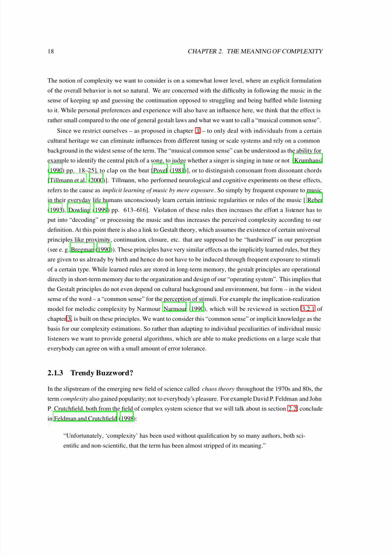
Since we restrict ourselves – as proposed in chapter 1 – to only deal with individuals from a certain
cultural heritage we can eliminate influences from different tuning or scale systems and rely on a common
background in the widest sense of the term. The “musical common sense” can be understood as the ability for
example to identify the central pitch of a song, to judge whether a singer is singing in tune or not [Krumhansl
(1990) pp. 18–25], to clap on the beat [Povel (1981)], or to distinguish consonant from dissonant chords
[Tillmann et al. (2000)]. Tillmann, who performed neurological and cognitive experiments on these effects,
refers to the cause as implicit learning of music by mere exposure. So simply by frequent exposure to music
in their everyday life humans unconsciously learn certain intrinsic regularities or rules of the music [Reber
(1993), Dowling (1999) pp. 613–616]. Violation of these rules then increases the effort a listener has to
put into “decoding” or processing the music and thus increases the perceived complexity according to our
definition. At this point there is also a link to Gestalt theory, which assumes the existence of certain universal
principles like proximity, continuation, closure, etc. that are supposed to be “hardwired” in our perception
(see e. g. Bregman (1990)). These principles have very similar effects as the implicitly learned rules, but they
are given to us already by birth and hence do not have to be induced through frequent exposure to stimuli
of a certain type. While learned rules are stored in long-term memory, the gestalt principles are operational
directly in short-term memory due to the organization and design of our “operating system”. This implies that
the Gestalt principles do not even depend on cultural background and environment, but form – in the widestsense of the word – a “common sense” for the perception of stimuli. For example the implication-realization
model for melodic complexity by Narmour Narmour (1990), which will be reviewed in section 3.2.1 of
chapter 3, is built on these principles. We want to consider this “common sense” or implicit knowledge as the
basis for our complexity estimations. So rather than adapting to individual peculiarities of individual music
listeners we want to provide general algorithms, which are able to make predictions on a large scale that
everybody can agree on with a small amount of error tolerance.
2.1.3 Trendy Buzzword?
In the slipstream of the emerging new field of science called chaos theory throughout the 1970s and 80s, the
term complexity also gained popularity; not to everybody’s pleasure. For example David P. Feldman and John
P. Crutchfield, both from the field of complex system science that we will talk about in section 2.2, conclude
in Feldman and Crutchfield (1998):
“Unfortunately, ‘complexity’ has been used without qualification by so many authors, both sci-
entific and non-scientific, that the term has been almost stripped of its meaning.”
7/29/2019 Streich, S. (2007). Music Complexity. a Multi-faceted Description of Audio Content. Universitat Pompeu Fabra.
http://slidepdf.com/reader/full/streich-s-2007-music-complexity-a-multi-faceted-description-of-audio 36/124
2.2. THE FORMAL VIEW 19
Looking at the 386 entries for publications on complexity measures from so different fields as Psy-
cholinguistics, Urban Geography, and Mathematical Economics in an on-line database from the year 1997
[Edmonds (1997)] gives us an idea of what Feldman and Crutchfield are talking about. But what exactly
makes the term so attractive? Is it just its modern and scientific sound, is it simply a “trendy buzzword”?
Again, we can find some insight by looking at the writings of Edmonds (1995):
“The label ‘complexity’ often performs much the same role as that of the name of a desirable
residential area in Estate Agent’s advertisements. It is applied to many items beyond the original
area but which are still somewhere in the vicinity.”
So, according to Edmonds there seems to be indeed some buzzword characteristic about the term “com-
plexity”. He gives a few examples of what falls into this “vicinity”:
Size is an indication of the general difficulty in dealing with the system/object and therefore rather the po-tential of it being complex.
Ignorance can be caused by high complexity, but it is not equivalent to it.
Minimum description size is related with the amount of information (see 2.2); while the absence thereof
will coincide with the absence of complexity the inverse is not necessarily true, since the component
of interrelation increases complexity but might reduce the amount of information.
Variety again is necessary for complexity to emerge, but by itself not sufficient for it.
Order and disorder are also closely related with complexity, but Edmonds argues that they need a language
of representation in order to become tractable (see the explanations for figures 2.1 and 2.2).
Complexity is so suitable as a grouping term, because it has no well established and widely accepted
definition and it is strongly associated with several related concepts. But as we saw it cannot simply be
reduced to any of them and it is necessary to treat it as a separate, self-contained idea. It is however only an
advantage for our purposes, if the term can be used with academic precision and at the same time is roughly
understandable by outsiders or laymen without lengthly explanations.
2.2 The Formal View
In certain fields of science complexity plays a special role and makes a formal expression necessary. Forour needs it is sufficient to provide a verbal definition of what we want to consider as our target and then
start from there to develop and explore different algorithmic approaches. While an all-round mathematical
formula for complexity is not our ultimate goal, it is still interesting to look at the different definitions in
order to learn about ways how complexity can be approached computationally and what problems occur. The
list of reviewed measures is far from completeness and merely serves illustrative purposes by providing a few
selected, popular examples.

7/29/2019 Streich, S. (2007). Music Complexity. a Multi-faceted Description of Audio Content. Universitat Pompeu Fabra.
http://slidepdf.com/reader/full/streich-s-2007-music-complexity-a-multi-faceted-description-of-audio 37/124
20 CHAPTER 2. THE MEANING OF COMPLEXITY
2.2.1 Information and Entropy
In the view of information theory a sequence of data is a message that can be transmitted from a source
through a channel to a receiver. The message contains information, a quantifiable property, which is measured
in bits. In fact, what needs to be transmitted really is only this information, and one can “repackaged” it more
tightly in a smaller message if possible to save bandwidth or storage space. If we consider a source that is
always sending messages of the same type, then we can calculate the average amount of information that this
source emits with every symbol. This concept is called the source entropy. It was introduced by Shannon
(1948) and is probably the most “traditional” measure from the field of information theory that can be related
with complexity. Intuitively we would attribute a lower complexity to a source that sends less information
per symbol, high entropy values would be associated with higher complexity, since the information rate is
higher. But what entropy measures is the randomness of the output from an information source, which is not
exactly the same as complexity (as we discussed already in the preceding sections). The average amount of
information for each symbol si emitted by a source can be calculated with the following formula:
H 0 = −N i=1
p(si) · log2 p(si), (2.1)
where N is the number of distinct symbols and p(si) is the probability that symbol si is emitted. Equation 2.1
assumes a memoryless source, like the flipping of a coin or the rolling of a dice, where the preceding symbol
in the sequence has no influence at all on the symbols to follow. This assumption is not justified in many
practical applications. For structured data as texts for example, the probability of a symbol depends strongly
on its predecessors. In information theory the terms Markovian source and Markov chain are used in these
cases. Equation 2.1 can be adapted for a Markov chain by taking the corresponding conditional probabilities
into account. If only the direct predecessor is relevant (as in a first order Markov chain), the equation takes
the following form:
H 1 = −N
i=1
p(si)N
j=1
p(sj |si) · log2 p(sj |si), (2.2)
where p(sj |si) denotes the conditional probability of symbol sj appearing after symbol si in the sequence.
H 0 is the upper bound for H 1 and any higher order entropy of a given source, since the structural regu-
larities captured by the conditional probabilities can only decrease randomness. One problem is therefore
to determine the proper order that should be used with a given sequence. Another problem, when consid-
ering musical audio signals is that they do not come readily as sequences of discrete symbols and the true
probability distributions are not known.
7/29/2019 Streich, S. (2007). Music Complexity. a Multi-faceted Description of Audio Content. Universitat Pompeu Fabra.
http://slidepdf.com/reader/full/streich-s-2007-music-complexity-a-multi-faceted-description-of-audio 38/124
2.2. THE FORMAL VIEW 21
2.2.2 Kolmogorov Complexity
The most widespread and most referenced definition of complexity in the information theory field originatesfrom the theory of algorithmic information. Referring to one of the main scientists behind it this defini-
tion is usually called Kolmogorov complexity [see Gammerman and Vovk (1999) for a short introduction].
In contrast to entropy it doesn’t address the average information transmitted by a source, but the absolute
information content of an object (a data string s). This quantity specifies the amount of data that needs to be
transmitted in the absence of any other a priori knowledge. It is defined as the length of the shortest program
p (in bits), that can generate the sequence s. Formally we can write:
K (s) = min(| p| : T ( p) = s), (2.3)
where T ( p) refers to the output of a universal Turing machine executing p. Thanks to its general natureKolmogorov complexity has been applied also in the digital audio domain (see Scheirer (2001)) as a way to
prove mathematically the advantages of structured audio in generalized audio coding.
The striking quality of both concepts is the objectivity of the measures. Kolmogorov complexity and
Shannon entropy both exist as exclusive properties of the object (data sequence or source) and are completely
independent from an observer. But when considering musical audio signals we face problems. First as
mentioned already, the entropy measure needs a finite set of discrete symbols being emitted from the source,
but this is not what we have. The audio signal would need to be converted somehow into symbols like
the letters in a written text, which is not very straightforward. Despite that music can be generated with a
keyboard it is usually much more than the output of a “typewriter” 4.
Secondly, both measures are rather technical focusing on an efficient encoding, while we are interested
in the reception by humans. A practical example illustrating this difference very well is given in Standish
(2001). He points out that a random sequence of numbers will always yield a maximum complexity although
it does not contain any meaningful information for a human. Comparing a random string of characters with
the manuscript of a theater play, the random sequence would yield the higher Kolmogorov complexity value,
because there is no program to generate the sequence shorter than the sequence itself. However, for a human
the order would be exactly reversed, because the random string is perceived as meaningless noise, while the
theater play is recognized as a sophisticated, multi-layered setting (at least if it is a good one). The apparent
objectivity of the measure makes it meaningless when context has to be considered as it is the case for the
goals of this research.
Standish suggests the use of equivalence classes to overcome this. An equivalence class for him is the
set of all mutations of a sequence that are equivalent in a given context. So for example different random
sequences could hardly be distinguished by a human observer and would therefore form a large equivalence
class. On the other hand, for a written text carrying a meaning, only relatively few mutations exist that would
be judged as equivalent. This judgement depends not only on the data itself but also the context in which
4This can be experienced easily by comparing a monophonic mobile phone ringing tone with a live performance of the same piece.

7/29/2019 Streich, S. (2007). Music Complexity. a Multi-faceted Description of Audio Content. Universitat Pompeu Fabra.
http://slidepdf.com/reader/full/streich-s-2007-music-complexity-a-multi-faceted-description-of-audio 39/124
22 CHAPTER 2. THE MEANING OF COMPLEXITY
it is observed. If the equivalence classes are considered in the complexity computation, we arrive at more
meaningful results from a human’s point of view. But still we do not have a practical solution. The decision
of what is equivalent and what is not does not seem to be very straightforward, especially when it comes to
music. Furthermore there is no closed mathematical solution for computing the Kolmogorov complexity and
it remains a rather theoretical measure.
Another extension of the idea behind Kolmogorov complexity is the so called logical depth proposed
by Bennett (1985). In short the idea behind this is to consider the number of computational operations that
are required to generate the sequence x with the minimal program as a measure of complexity. This is an
elegant way to deal with the problem of randomness, because for an incompressible random string the shortest
program will simply store the entire sequence and just do print(x). This means for the logical depth:
L(x) ≈ |x|. If the sequence is highly redundant and consists of periodic repetitions, the minimal program
will cycle over printing the same data for each period, which again leads to L(x) ≈ |x|. When there exists a
non-trivial minimal program that can generate a sequence it will involve more advanced computations than
simply reading each value from a list. So the number of operations will be bigger and L(x) > |x|. However,
the problem remains that there is no closed mathematical solution for finding the minimal program, which
makes the logical depth again useful in theory only.
2.2.3 Stochastic Complexity
There is an important difference between the information theoretic measures that we just reviewed and the
method we will discuss here. The former ones are concerned with an exact reproduction of the data sequence.
When we look at the minimal program as a type of model for the system that generated the data, this is an
extreme case of over-fitting5. If we consider the data as a series of measurements or observations that contains
some noise, then these methods pay way too much attention to details that are practically irrelevant. Instead
we should relax the degree of exactness and allow a certain tolerance due to noise, that can be described
easily in a statistical sense [Shalizi (2006)].
The most well-known method following this line of argumentation is the one proposed by Rissanen
[Rissanen (1978) and Rissanen (1989)] which uses the Minimum Description Length principle and the asso-
ciated stochastic complexity. The basic idea behind this is that there has to be a trade-off between the accuracy
of a model and how well it generalizes. The accuracy can always be increased by choosing a more complex
model. On the other hand, if we choose a simpler and therefore more general model, we will have to consider
a greater amount of noise to describe the data D. Figure 2.3 illustrates these effects. On the left a very simple
model (straight line) is chosen, which provides a poor fit to the data (dots). The noise component would be
very big in this case. In the center the model is very complex (high order polynomial function), while it fits
this data very well it probably not work very well on a different data sample from the same source/system.
On the right side we can see a compromise, the model fits reasonably well, but it is significantly simpler than
the one from the center and thus more general. So we have to consider two components when describing the
5Of course Information Theory is not concerned with any type of generalization.

7/29/2019 Streich, S. (2007). Music Complexity. a Multi-faceted Description of Audio Content. Universitat Pompeu Fabra.
http://slidepdf.com/reader/full/streich-s-2007-music-complexity-a-multi-faceted-description-of-audio 40/124
2.3. IMPLICATIONS FOR OUR GOALS 23
Figure 2.3: Example for model selection with Minimum Description Length [from Grunwald (2005)].
data with our model. L(M ) is the amount of bits needed to describe the model M , where a more complex
model will need more bits. L(D|M ) is the amount of bits we need to describe the “noisy” part of the data
when applying the model M . Since we don’t want to transmit this description it is enough for us to get an
estimate of the number of bits instead of defining the explicit encoding. The stochastic complexity of the data
is then defined as the minimum of L(M ) + L(D|M ) for all models under consideration.
Despite this approach has proven to be very useful for model selection, Shalizi (2006) points to several
shortcomings when we are interested in a measure of complexity. First, the outcome depends a lot on the
way we choose to encode the models. It is up to us to decide which types of models we want to have “under
consideration” and according to which method we encode them. Secondly, the “noisy” term L(D|M ) not
only reflects the true noise in the data, but also the imperfection of the chosen model. As Shalizi puts it, “it
reflects our ineptness as modelers, rather than any characteristic of the process.” Thirdly, one can question thephysical significance of the stochastic complexity, since in the system there is no need for a representation
of its organization. This is only necessary for us who have to choose from different models and to fix the
parameters.
2.3 Implications for our goals
So what are the implications of all the above for the goals we identified in section 1.2? By looking at
the different general complexity measures that exist, it emerges that these will not take us far, if our main
concern is a semantic description of music audio. Although it is always elegant to have a neat and general
mathematical formalism behind, it is not necessary in order to arrive at practically useful results. On the other
hand this doesn’t mean that it makes no sense to include ideas and principles from these measures into our
algorithms. We will review approaches in the following chapter that achieve interesting results by doing so.
But the point is, that we do not want to impose a general, theoretical model of complexity as a starting point
that is then simply applied to the complexity facets at hand.
While we are interested in developing algorithms that are capable of making meaningful predictions of

7/29/2019 Streich, S. (2007). Music Complexity. a Multi-faceted Description of Audio Content. Universitat Pompeu Fabra.
http://slidepdf.com/reader/full/streich-s-2007-music-complexity-a-multi-faceted-description-of-audio 41/124
24 CHAPTER 2. THE MEANING OF COMPLEXITY
human judgements it is not our concern to accurately model the underlying cognitive processes. It certainly
is helpful to include known principles of human perception and cognition in our implementations, but it is
not our ultimate goal to learn about these principles from our algorithms. If there is a simple implementation
that does the job roughly as well as a sophisticated one which is closer to the actual processing taking place
in our brains, then we would prefer the simple one for reasons of practicality.
So what we want to do is in fact a hybrid approach. We will look on one hand at the mechanisms at work in
the music “processing” behavior of humans as they are known and on the other hand at feasible computational
methods. The proposed algorithms are meant to provide a connection between the two. Additionally, we will
use the observations we made in section 2.1 to guide us in the algorithm development when the understanding
of the cognitive process is not advanced enough.

7/29/2019 Streich, S. (2007). Music Complexity. a Multi-faceted Description of Audio Content. Universitat Pompeu Fabra.
http://slidepdf.com/reader/full/streich-s-2007-music-complexity-a-multi-faceted-description-of-audio 42/124
Chapter 3
Former Work on the Complexity of
Music
After the subject of our research has been explained and specified, and the intended applications have been
described, we will now have a closer look at the work that has already been done in this area. We will first
review several experimental findings in the context of Berlyne’s theory of arousal potential [Berlyne (1960)
and Berlyne (1971)]. Then we will address different approaches on modelling and computing complexity
facets of music that have been published by other researchers. We will focus here mainly on the methods
that analyze music in terms of complexity, neglecting those utilizing complexity for automatic generation or
composition [for some examples see Dobrian (1993), Hodgson (2006), or Goertzel (1997)], as they are not inthe focus of our thesis.
3.1 The Preferred Level of Complexity
We pointed out in section 1.3 that according to Berlyne’s theory of arousal potential [Berlyne (1971)] the
level of perceived complexity of a piece of music can be associated with the preference for it. Our research is
not intending to provide evidence for the validity of this theory. Exploiting the psychological aspects between
perceived complexity and preference is not our main concern. However, this aspect plays an important role
in the motivation for our research. Hence, we want to give some room here to report about material that has
been published on the matter.
3.1.1 Complexity and Aesthetics
Berlyne himself conducted several studies during the 1960s and 1970s [ Berlyne (1960), Berlyne (1971), and
Berlyne (1974)] on the connection between arousal potential and hedonic value (liking) of artistic stimuli.
He has considered not only auditory, but also visual and combined stimuli in his experiments. He has found
25

7/29/2019 Streich, S. (2007). Music Complexity. a Multi-faceted Description of Audio Content. Universitat Pompeu Fabra.
http://slidepdf.com/reader/full/streich-s-2007-music-complexity-a-multi-faceted-description-of-audio 43/124
26 CHAPTER 3. FORMER WORK ON THE COMPLEXITY OF MUSIC
strong evidence for the existence of the inverted-U relationship as depicted in figure 1.3 on page 9 which led
to his theory of arousal potential. As mentioned above he identified different types of variables to contribute
to arousal potential [Berlyne (1960) pp. 170–179]:
• Intensive Variables (e. g. pitch, color, energy)
• Affective Variables (e. g. anxiety, pain, gratification)
• Collative Variables (e. g. novelty, surprisingness, complexity)
Berlyne considered the collative variables the most important ones of the three types. His understanding of
complexity is very closely linked to information theory and the formal measures presented in section 2.2.1.
In Berlyne (1971) on page 149 he says:
“A pattern is considered more complex, the larger the number of independently selected elements
it contains. In two patterns that consist of the same number of elements, that one will be less
complex that has a greater degree of similarity among its elements or, more generally, a greater
degree of redundancy of interdependence.”
Later, from his extensive review of experiments he draws the more general conclusion that “[. . . ] with sound
sequences as with visual patterns, subjective complexity reflects information content.” [ib. p. 202].
For art, Berlyne resumes, one has to distinguish between two groups of qualities, one around the terms
beauty and pleasingness and a distinct one linked with the term interestingness. As he shows by reporting
the results of numerous studies [ib. pp. 198–213] the latter usually increases with increasing complexity
while the former tends to be higher for stimuli with relatively low complexity. This coincidence of beauty
and simplicity is also put forward by Schmidhuber (1997). He even proposes a new art form called “Low-
Complexity Art” joining the formal measures of Kolmogorov Complexity and minimum description length
with the process of artistic production. He suggests that what can be described very efficiently in terms of
an internal representation by the observer, will also be considered beautiful. He gives the example of human
faces, where an average, prototypical, symmetrical face is considered more beautiful than an “irregular” one,
that would need more effort in the internal modelling process. Both, Schmidhuber and Berlyne, recognize
however, that the most beautiful and pleasing is not necessarily the preferred choice, because it might be rather
uninteresting. So an optimal choice would be at the same time beautiful and interesting and thus somewhere
between total order and randomness. Following Berlyne’s theory, if we take again the three diagrams of
figure 2.1 from page 2.1 we could expect people to prefer the middle one. If we presented the three diagrams
individually to subjects and allowed them to switch freely forward and backward, we should observe that
they spend more time looking at the middle one than at the other two.
3.1.2 Psychological Experiments
With respect to music complexity in particular, Heyduk (1975) reports about an experiment with four custom-
built piano compositions of different complexity levels. Complexity was varied in two facets: chord structure

7/29/2019 Streich, S. (2007). Music Complexity. a Multi-faceted Description of Audio Content. Universitat Pompeu Fabra.
http://slidepdf.com/reader/full/streich-s-2007-music-complexity-a-multi-faceted-description-of-audio 44/124
3.1. THE PREFERRED LEVEL OF COMPLEXITY 27
and syncopation. He found strong evidence for Berlyne’s theory by analyzing the ratings for preference
and complexity given by a group of 120 subjects. While Berlyne used the term arousal potential for the
combination of different factors determining preference, Heyduk follows the terminology of Walker (1973)
and talks about psychological complexity. It is important to note the distinction to a pure stimulus complexity
here. The latter would be fixed and objective, very much like the Kolmogorov complexity mentioned in
section 2.2.2. The psychological complexity includes the latter, but is also determined by attributes like
novelty, uncertainty and arousal properties. It doesn’t exist without specifying a specific observer. It therefore
is a subjective property, which only becomes manifest in the encounter of an individual with the stimulus.
Steck and Machotka (1975) conducted an experiment using random sequences of sinusoidal tones as
stimuli. All tones were equally loud and had equal duration within one “composition” of approximately 10s
length. 16 different levels of complexity were constructed by varying the tone duration (and thus the tone
rate) from 2s down to 60ms. The analysis of preference ratings from 60 subjects revealed a clear inverted-Urelationship on the objective complexity levels. However, when presenting only subsets of the test samples
which were taken from adjacent complexity levels, again an inverted-U relationship was found within each
subset. Even more interesting is their observation that the relative position of maximal preference inside each
subset was fixed. That means the preferred level of complexity was not absolute, but relative for the presented
stimuli.
North and Hargreaves point to two potential problems with respect to Berlyne’s theory: the influence of
the listener’s mood and intention when selecting music, and the dependence on the appropriateness of the
music for the listening situation [North and Hargreaves (1997a)]. It seems obvious that the same listener will
prefer different types of music whether he is driving a car, relaxing on the sofa, or dancing in the club. So
when they asked subjects to rate the preference for the music in a cafeteria, they indeed found an inverted-U
shaped relation between complexity and preference. However, the effects were mediated by musical style.
Organ music of the same complexity level as New Age music was liked less in this listening situation. In
another study North and Hargreaves (1997b) show that preference and pleasantness of music have to be dis-
tinguished. Preference and arousal potential were again found to relate through the inverted-U curve in this
study. But North and Hargreaves argue that a subject with an antipathy against brass music for instance will
not be pleased by this music, whether it matches the optimal complexity level or not. In this sense, optimal
complexity only provides the potential for a maximum of pleasure a subject might experience, but does not
determine it completely. Conversely, a subject might find pleasure in listening to music that does not pos-
sess the optimal level of complexity. However, pleasure would reach a maximum when the right level of
complexity and a general liking coincide in a piece of music.
A quite recent study by Orr and Ohlsson (2005) addressed the dependency of musical expertise on pref-
erence. They used natural stimuli, bluegrass and jazz solos, at different complexity levels, which were pur-
posely performed and recorded for their experiments. Four different groups of subjects were asked to rate
perceived complexity and liking for the stimuli. One group consisted of subjects with no musical training, a
second one was composed of subjects with moderate training in music, the third and fourth group consisted
7/29/2019 Streich, S. (2007). Music Complexity. a Multi-faceted Description of Audio Content. Universitat Pompeu Fabra.
http://slidepdf.com/reader/full/streich-s-2007-music-complexity-a-multi-faceted-description-of-audio 45/124
28 CHAPTER 3. FORMER WORK ON THE COMPLEXITY OF MUSIC
of professional jazz and bluegrass musicians. The results reported by Orr and Ohlsson indicate two things.
First, it seems that the significance of complexity for preference decreases with increasing musical expertise,
unless complexity itself is learned as an aesthetic criterion. This can be seen from the fact that for the group of
professional jazz musicians an inverted-U relationship could not be identified. For the professional bluegrass
musicians the inverted-U relationship only appeared for their ratings of bluegrass music. The authors interpret
this effect insofar as complexity might represent an explicit aesthetic criterion in bluegrass music, which has
been learned by the professionals. The group of untrained subjects was the one where the inverted-U became
apparent the most for either musical style. The moderately trained group revealed this effect only in case of
the bluegrass samples. So secondly, the importance of optimal complexity seems also to depend on the music
style. We have reviewed so far only psychological studies using selected stimuli where the complexity was
purposely varied in a controlled test environment. It is also interesting to consider studies that were conceived
the other way around, that means observing preference indicators of real music and then relating these with
complexity estimations.
3.1.3 Musicological Studies
Eerola and North (2000) report about their analysis of 128 Beatles songs, all written by and for the Beatles
in the years between 1962 and 1970. From MIDI-transcriptions of the songs they extracted the melodies and
analyzed the melodic complexity with their expectancy-based model (see section 3.2.1). A highly significant
increasing trend was found for melodic complexity over the time period. Secondly, the authors compared the
complexity values with indicators of commercial success of the songs and albums. The chart position and the
time in the charts were both negatively correlated with melodic complexity. So the higher the complexity,
the less popular were the songs. Although this is a sign of relevance between complexity and popularity, the
authors point out that other factors of social, cultural, or commercial kind certainly have an influence as well.
Since they were not considered in the study, care has to be taken in drawing conclusions. A shortcoming of
this study is also that it was not checked whether the increase in complexity was a general trend during that
time period or whether this was only observed in the music of the Beatles. However, they make reference to
Simonton (1994), who also found a clear connection between melodic complexity and popularity. His results
stem from an extensive study of 15,618 melodic themes of classical music.
A study by Parry (2004) comes to similar conclusions. He analyzed the melodic and rhythmic complexity
of 10 songs that were listed in the Billboard Modern Rock Top 40 within the period from January to June
of 1996. The complexity was estimated using MIDI transcriptions of the songs and is based on a very basicself-similarity measure. As indicators for the chart performance the number of weeks in the charts, average
weekly change in rank, peak ranking, and debut ranking were considered. Parry found the number of weeks
in the charts being positively correlated with both, rhythmic and melodic complexity. The former was also
positively correlated with the peak ranking. For the average change in rank a negative correlation was found
with melodic complexity, indicating that higher melodic complexity inhibited rapid changes. The debut
ranking revealed no statistically significant correlation with the two complexity measures.

7/29/2019 Streich, S. (2007). Music Complexity. a Multi-faceted Description of Audio Content. Universitat Pompeu Fabra.
http://slidepdf.com/reader/full/streich-s-2007-music-complexity-a-multi-faceted-description-of-audio 46/124
3.2. COMPUTING COMPLEXITY ON SYMBOLIC REPRESENTATIONS 29
3.1.4 Conclusion
As a conclusion we can say that a certain relationship between preference and complexity of music cannot bedenied. Based on the rather scarce evidence the correlation, however, seems to be not as simple as it appears
in Berlyne’s theory. Other factors, as mentioned, also show effects and might under certain circumstances
completely overrule the influence of complexity on preference. It should therefore not be expected to have
found the holy grail of music recommendation with the usage of complexity descriptors. On the other hand,
the reported findings clearly prove the relevance of complexity in music listening, especially for non-expert
listeners, which are the target audience we are considering. Providing complexity descriptors for music there-
fore should be able to enhance human interaction with music collections, which is the goal of the research
presented here.
3.2 Computing Complexity on Symbolic Representations
There exists a substantial amount of publications on facets of music complexity based on the analysis of
score-like representations. Mostly, the focus lies on high-art music in the western cultural tradition. While
we include this type of music as well into our pool of musical material, it rather forms a niche in the context of
popular music that we want to process with our methods. Furthermore we have to distinguish between the ap-
proaches that make use of expert knowledge of a theoretical nature and those that rely only on subconscious,
cognitive effects in the listener. In David Temperley’s terminology the former belong to the suggestive type of
musicology, while the latter – which are more interesting for us – belong to the descriptive type [Temperley
(2001b)]. For each presented approach we will also discuss to which degree it might be applied to our
problem, which deals with music in the form of audio signals.
3.2.1 Models for Melodic Complexity
Already back in 1990 Eugene Narmour proposed a model for the complexity of melodies that clearly falls
into the descriptive category. This Implication-Realization model, as he calls it, is extensively described
in Narmour (1990). The model hierarchically builds up larger structures from smaller elements and thus
possesses different levels. The predictions are most clearly specified on the lowest level, which is the tone-
to-tone level. Any melodic interval that is perceived as being “open” (incomplete sounding) is said to create
an implication on the listener’s side. That means it raises certain expectations in the listener about how the
sequence is supposed to continue. Factors that contribute to closure (i. e. the opposite of openness) at the
single-interval (tone-to-tone) level are [Schellenberg et al. (2002)]:
• a longer duration of the second tone than the first one (e. g. eighth note followed by quarter note)
• a higher stability of the second tone in the established musical key (e.g. ti followed by do)
• a stronger metrical emphasis of the second tone (e. g. at the first beat of a measure).

7/29/2019 Streich, S. (2007). Music Complexity. a Multi-faceted Description of Audio Content. Universitat Pompeu Fabra.
http://slidepdf.com/reader/full/streich-s-2007-music-complexity-a-multi-faceted-description-of-audio 47/124
30 CHAPTER 3. FORMER WORK ON THE COMPLEXITY OF MUSIC
Figure 3.1: Illustration of the Implication-Realization Process [from Schellenberg et al. (2002)].
According to these criteria a melodic sequence can be segmented and we can observe to which degree
the implications evoked by the “open” intervals are realized. For example a relatively small interval (that is
perceived as being “open”) would make the listener expect a continuation by another small interval in the
same direction. A large interval would raise the expectation for a small interval in the opposite direction.
Frequent realization of these expectations reveals a low level of complexity; frequent surprises reveal a high
level of complexity, because the structure of the melody is harder to encode.
Figure 3.1 illustrates exemplary the implications for the tone-to-tone level. The first interval implies a
second one to follow, while the relative thickness of the arrows indicates that different continuations can be
implied with different strength.
It has to be pointed out that the development of this model was guided by gestalt principles only, implying
validity completely independent from the listener’s cultural or musical background. Narmour himself states
about the principles that they are “innate, hardwired, bottom-up, brute, automatic, subconscious, panstylistic,
and resistant to learning” [as cited by Schellenberg et al. (2002)].
The IR-model inspired many experiments. It was reduced by Schellenberg to its basic principles. In
experiments with human listeners Schellenberg used artificial stimuli and original folksong melodies. By
comparing the explanatory power of his simplified model with Narmour’s original he proved experimentally
that both versions give similar results [Schellenberg (1996)].
7/29/2019 Streich, S. (2007). Music Complexity. a Multi-faceted Description of Audio Content. Universitat Pompeu Fabra.
http://slidepdf.com/reader/full/streich-s-2007-music-complexity-a-multi-faceted-description-of-audio 48/124
3.2. COMPUTING COMPLEXITY ON SYMBOLIC REPRESENTATIONS 31
In section 3.1.3 we mentioned already a model for melodic complexity by Eerola and North. In Eerola and North
(2000) they point out that the traditional information theorist view of complexity does “not address the role of
the listener’s perceptual system in organising the structural characteristics of music”. Therefore they propose
their expectancy-based model (EBM) to estimate complexity. It is also inspired by Narmour’s ideas, but they
include some additional features derived from a symbolic representation of the music. In their evaluation
they found that tonality (modified by metrical position and tone duration), the intervallic principles registral
direction and intervallic difference, and the rhythmic principles syncopation and rhythmic variability showed
significant capability in predicting listeners’ complexity judgements. Comparing the prediction accuracy of
this model with an information-theoretic and a transition probability model [Simonton (1984)], they found it
to be the best one.
Eerola et al. (2002) conducted experiments showing, how the accuracy of the model can be further im-
proved by taking a larger melodic context into account. Since the focus of the original model is limited totwo notes at a time only, it neglects the impact of the longer-term melodic evolution (e. g. repetition of mo-
tives) on the listeners’ predictions of continuation. However, their modifications were aiming more towards
a real-time modelling of listeners’ continuation predictions than towards a more accurate estimation of the
overall complexity.
In sum we can say that there is a selection of computable models available, that have shown reasonably
good performance in approximating human impressions of melodic complexity. However, there is one obsta-
cle that makes it difficult to apply these methods to the problem we are tackling: All the presented models
are working on a symbolic representation of the melody. This is disadvantageous for us in two ways. First,
simply for pragmatical reasons, because digital music files do not have this symbolic description attached
to them. Although there is a lot of active research going on aiming at the complete transcription of musical
audio [e. g. Klapuri (2004) or Bello (2003)] or precisely at the extraction and transcription of the melodic
voice [e. g. Dressler (2005)], the results are still far from being useable. The best algorithm for melodic
pitch tracking in polyphonic signals in the 2004 ISMIR contest achieved only an average accuracy of 75%
[Gomez et al. (2005)]. This figure does not even include note segmentation. The task is so difficult, because
it involves several steps which each by itself tend to introduce errors to the computational result. Out of the
polyphonic signal the fundamental frequencies of the sounding notes need to be detected, while the number
of sounding notes is not known. For each note the onset and offset has to be identified, which might be
obscured by unstable fundamental frequencies and non-tonal elements in the music. Finally from all detected
sounding notes the ones that form the melody have to be selected, while the criteria for this selection are not atall clear. Just a few wrong notes in the extracted melody, however, would completely mislead the complexity
estimation with the presented models making the application useless. Secondly, it must be asked, whether
the perception of melodic complexity should be considered independently from the accompaniment. While
the reported methods only deal with isolated, monophonic melodies, we are interested in describing complete
musical arrangements. It could be the case that the findings on human complexity perception regarding the
former are not directly applicable to the latter.

7/29/2019 Streich, S. (2007). Music Complexity. a Multi-faceted Description of Audio Content. Universitat Pompeu Fabra.
http://slidepdf.com/reader/full/streich-s-2007-music-complexity-a-multi-faceted-description-of-audio 49/124
32 CHAPTER 3. FORMER WORK ON THE COMPLEXITY OF MUSIC
3.2.2 Models for Rhythmic Complexity
In Shmulevich and Povel (2000) the PS-measure for rhythmic complexity was introduced. The authors state,with reference to Essens (1995), that a listener tries to establish an internal clock, when hearing rhythmic
music. According to this clock the listener then segments the rhythm pattern and tries to code the segments.
So a rhythmic pattern will appear complex, when either the induction of the internal clock is weak or ab-
sent, or when the coding of the segments is difficult. The algorithm therefore combines the two aspects for
complexity estimation.
The clock induction strength is a weighted combination of the number of clock ticks that coincide with
silence and with unaccented events. This shows already, that a rather high abstraction level is assumed here,
since the clock grid is assumed to be known and the musical events have to be classified into accented,
non-accented, and silent ones.
The coding complexity is estimated by assigning different weights to four different types of segments
that can appear when splitting up the sequence of events according to the clock grid. The segment types are
empty segments, equally subdivided segments, unequally subdivided segments, and segments beginning with
silence. An additional weight exists that is added, when two consecutive segments differ from each other.
The coding complexity is then simply the sum of all the weights for the whole sequence.
Shmulevich and Povel (2000) tested their method on a set of 35 rhythm patterns for which they obtained
human complexity judgments in a listening test. For comparison they also used the T-measure proposed by
Tanguiane (1993) and a pure information theoretic measure [Lempel and Ziv (1976)]. The former counts the
number of distinct “root patterns” in a sequence that would be needed for its generation, where elaborations
of these root patterns do not add complexity. The latter is based on the number of distinct substrings that
are found as the sequence evolves. The results showed that the PS-Measure gave clearly the best approx-
imations of the human ratings with an overall correlation coefficient r = 0.75 for the 35 tested patterns.
Shmulevich and Povel (2000) attribute this to the fact that their measure incorporates perceptual information
and is based on an empirically tested model.
It must be noted that the clock induction strength and the coding complexity when computed this way
tend to give higher complexity ratings to longer segments, because there is no normalization. This might be
appropriate when isolated rhythm patterns are evaluated, since a longer pattern is supposed to have a higher
complexity potential than a short one. However, for complete music tracks some adaptation would be in
need. It would be necessary to identify recurring rhythmic patterns throughout the piece and to segment
it accordingly. The measure could then be computed on each pattern and the overall complexity could be
approximated by combining the individual results in some intelligent way. This combination is not so straight
forward however. Might we consider that the perceived complexity decreases if listeners are exposed to one
single pattern over and over again? And vice versa, is the result perceived as being more complex if we have
a sequence of many different patterns that by themselves are not extremely complex?
But these problems are not the most immediate ones we encounter when we consider to apply the PS-
measure in our context. Although rhythm pattern extraction from musical audio might seem an easier task

7/29/2019 Streich, S. (2007). Music Complexity. a Multi-faceted Description of Audio Content. Universitat Pompeu Fabra.
http://slidepdf.com/reader/full/streich-s-2007-music-complexity-a-multi-faceted-description-of-audio 50/124
3.2. COMPUTING COMPLEXITY ON SYMBOLIC REPRESENTATIONS 33
to solve compared with melody extraction, to date universal methods providing sufficient precision are still
lacking [a recent review can be found in Gouyon and Dixon (2005)]. The problem is again that errors can be
introduced at several different steps. Starting from the audio signal the onset times of rhythmic events have
to be identified, which will result in several false detections and missed onsets. Based on the inter-onset-
intervals or additional features the beat has to be tracked [referred to as “the clock” by Shmulevich and Povel
(2000)], which is not necessarily stable throughout the entire piece. The PS-measure is an essentially “binary”
measure. A rhythmic event either is accented or not, it either coincides with a clock tick or not. While this
comes rather naturally with symbolic data, for real-world signals we need to apply thresholds and quantization
in order to make such decisions, and the outcome of the entire process depends strongly on the specification
of these thresholds. In summary, the application of the PS-measure in the context of real-world, polyphonic
audio appears to be not viable at present and was therefore left aside in this research work.
3.2.3 Models for Harmonic Complexity
The theory of harmony in music has a very long tradition already. Still, in contrast to melodic complexity,
no dominant and well-studied models for harmonic complexity could be identified by the author. Research
has been done on the expectations evoked in listeners by harmonic progressions especially on the field of
classical music [Schmuckler (1989)]. It turned out, that listeners usually predict a chord that results from
a transition considered as common in the given musical context. Yet, to our knowledge no tests have been
carried out that correlated the perceived harmonic complexity with the fulfilment or disappointment of these
expectations.
A step into this direction is done by Lerdahl (2001), who develops a hierarchical model for the perception
of tonal tension and chord distances in experienced listeners. Building up on the older “Generative Theory of
Tonal Music” [Lerdahl and Jackendoff (1983)] and integrating newer ideas [like Lerdahl (1996)], the model
relies on a rule-based grammar which we will not discuss in detail here. For a given sequence of chords it is
then possible to compute for example the overall distance that is “travelled”, which again can be related with
the complexity of the chord sequence.
A further extension of this idea can be found in Temperley (2001a). He supposes that the scores computed
with his preference rule system could reveal an estimate for the tension in music ( Temperley (2001a) section
11.5, pp. 307–317). The mapping of achieved scores would go from incomprehensible (breaking all rules)
over tense to calm, and finally to boring (all rules obeyed). Although he does not use the term complexity,
this basically reflects what we are looking for. He names four different aspects of this harmonic complexity:
1. The rate at which harmonies change.
2. The amount of harmonic changes on weak beats.
3. The amount of dissonant (ornamental) notes.
4. The distance of consecutive harmonies in a music theoretical sense.

7/29/2019 Streich, S. (2007). Music Complexity. a Multi-faceted Description of Audio Content. Universitat Pompeu Fabra.
http://slidepdf.com/reader/full/streich-s-2007-music-complexity-a-multi-faceted-description-of-audio 51/124
34 CHAPTER 3. FORMER WORK ON THE COMPLEXITY OF MUSIC
Especially the fourth point has to be addressed carefully when extending the scope from classical music
to the different types of modern popular music. Temperley himself considers this tension estimation to be
consistent only for particular styles (see Temperley (2001a) figure 11.11 p. 314). As we already discussed for
the model for melodic complexity (section 3.2.1) we again face the problem that an accurate chord transcrip-
tion is not easy to obtain from the audio signal. In the case of Temperley’s approach we face the additional
difficulty, that not only the pitches have to be transcribed, but also the rhythmic grid needs to be established
in order to distinguish between chord changes on strong and weak beats.
A different approach in the domain of harmonic analysis is taken by Pachet (1999), who proposes the
application of what he refers to as rewriting rules. He addresses the effect of harmonic surprise in Jazz music.
His argument is that the “rich algebraic structure underlying Jazz chord sequences” has to be considered when
talking about expectation and surprise. The idea is that a sequence of chords can be rewritten by applying a
limited set of rules to replace a particular chord in the sequence by one or more alternative ones.
His model is therefore based on two ingredients, a set of typical patterns, which he relates to the charac-
teristics of the musical style, and a set of rewriting rules, according to which a given chord sequence can be
transformed. The basic idea is that even a chord sequence that has never been heard before might not be so
surprising to a listener who is familiar with these two sets that are sufficient to generate it.
Instead of manually creating the two sets, Pachet applies machine learning techniques in order to obtain
them. He uses a string compression algorithm [Ziv and Lempel (1978)] in order to extract the typical pat-
terns. To find the rewriting rules he then uses a table method and utilizes the likelihood of occurrence of a
hypothesized rule as a basis for finding the best set of rewriting rules.
Although he is not directly aiming at a complexity estimation, the idea is not too far from our needs. A
highly predictable (little surprising) chord sequence could be identified with a low harmonic complexity andvice versa. However, Pachet focusses only on a very restricted variety of music, the Jazz genre, which is not
what we want. Also, he considers only a special type of expert listener, who is trained or accustomed to this
musical style. In addition, we have of course again the problem to obtain an accurate chord transcription from
the audio material before we can start to use Pachet’s ideas.
3.2.4 Pressing’s Music Complexity
Pressing (1998) gives a very short outline of three different types of complexity, which he names hierarchical,
adaptive, and generative or information-based complexity. Referring to music the first is focussing on the
structure of a composition. Pressing mentions Johann Sebastian Bach’s Kunst der Fuge as an example wherethe composer exploits hierarchical complexity. “[N]otes function as elements of linear processes operating
at different time scales, and are at the same time compatible with a vertically-oriented chordal progression
process.” He emphasizes that hierarchical complexity plays an important role in music composition, because
it allows a multiplicity of references increasing the potential for repeated listening and providing access at
different levels of sophistication. The second type of complexity refers to the temporal changes in a musical
work, including aspects like the adaption to unpredictable conditions, or the anticipation of changes in the

7/29/2019 Streich, S. (2007). Music Complexity. a Multi-faceted Description of Audio Content. Universitat Pompeu Fabra.
http://slidepdf.com/reader/full/streich-s-2007-music-complexity-a-multi-faceted-description-of-audio 52/124
3.2. COMPUTING COMPLEXITY ON SYMBOLIC REPRESENTATIONS 35
music itself or in the environment. Here, Pressing mentions improvisatory performance as an example. He
does not provide any details about how these two types of complexity could be addressed formally or even
computationally in practise.
The third type, the information-based complexity, is elaborated in some more detail by Pressing. It is
inspired by Kolmogorov complexity, but focuses more on the production of music through a human than on
the generation of a data string through a computer program. Pressing acknowledges that a pure information
theoretic measure falls short in measuring music complexity, because it will always rate random sequences
as the most complex ones, which does not go along with human perception. He argues that humans process
complexity by developing routines and heuristics that try to overcome the limitations of memory and atten-
tion. His approach to complexity is based on the concept that these routines have different difficulty levels,
because some are easier to learn than others. So conversely, the complexity of a stimulus is determined by
the difficulty assigned to the routines and heuristics that are needed to produce it.
He demonstrates his concept by estimating the complexity of six very short rhythmical patterns. This
is achieved by simply applying a processing cost function (cognitive cost) to the symbolic level attribute
syncopation on quarter-note and eight-note level. His approach shows some similarity with the coding com-
plexity used in the PS-measure for rhythmic complexity (section 3.2.2). Again, the sequence of events is
broken down into segments (this time according to two different grids) and a cost is assigned to each segment
depending on the type of syncopation that can be found.
This approach is very interesting, because it seems a convincing combination of information theoretic
principles and cognitive effects. However, it is purely theoretical and was not evaluated in any experiment
with humans, although Pressing states that a similar strategy is implemented in the notation software Tran-
scribe in order to achieve a cognitively optimal musical notation [Pressing and Lawrence (1993)]. Also thereis a crucial point in the identification of the routines and heuristics needed to generate the stimulus, as well
as in the assessment of cognitive costs to them. In the case of a complex musical audio signal this is a very
hard task to solve.
3.2.5 Algorithmic Clustering
While not a genuine measure of complexity, the algorithmic clustering of music proposed by Cilibrasi et al.
(2004) is still worth mentioning at this point, because it shows a practical application of information theoretic
principles applied to music. Cilibrasi et al. make use of the notion of compressibility that is linked with Kol-
mogorov complexity. They developed the normalized information distance as a universal similarity metric,
which they apply to symbolic representations of music in order to identify clusters of similar tracks in small
collections1.
In addition to the Kolmogorov complexity K (x) of a sequence x, they introduce the conditional com-
plexity K (x|y), which reflects the amount of information that is needed to reconstruct x if the sequence y is
1They report their method does not work as well for larger sets of musical pieces as it does for small ones [Cilibrasi et al. (2004)].

7/29/2019 Streich, S. (2007). Music Complexity. a Multi-faceted Description of Audio Content. Universitat Pompeu Fabra.
http://slidepdf.com/reader/full/streich-s-2007-music-complexity-a-multi-faceted-description-of-audio 53/124
36 CHAPTER 3. FORMER WORK ON THE COMPLEXITY OF MUSIC
Figure 3.2: Tree obtained with algorithmic clustering of 12 piano pieces [from Cilibrasi et al. (2004)].
given. The normalized information distance between x and y is then defined as:
d(x, y) =max(K (x|y), K (y|x))
max(K (x), K (y))(3.1)
This distance measure captures the number of bits of information that is not shared between the two se-
quences in relation to the maximum number of bits that could be shared [ Cilibrasi et al. (2004)]. Since the
Kolmogorov complexity is uncomputable in practice, it can only be approximated. Cilibrasi et al. (2004) use
standard file compression tools for this purpose. After the distances between all pairs of music files are com-
puted, Cilibrasi et al. (2004) use a tree-based clustering, called the quartet method , in order to identify groups
of similar songs. Although they claim this method to be a universal and feature-free similarity assessment,
they do need to represent the music as a discreet sequence of symbols in order to be able to compute the
distances. For this reason they use only the note on and note off information extracted from MIDI files in
their experiments. Timbre, tempo, and loudness information therefore have no effect on the distance compu-tation. Figure 3.2 shows the resulting tree obtained with the algorithmic clustering method for 12 classical
piano pieces from 3 different composers (2 fugues and 2 preludes from Bach, 4 Preludes by Chopin, and
the 4 movements from Suite Bergamasque composed by Debussy). Bearing in mind that there is no musical
knowledge or heuristics explicitly entered in the system at any point, the results are astonishing. Indeed the
method manages to separate the three composers quite well and it even groups the two fugues separately from
the two preludes inside the Bach cluster. Only Chopin’s prelude no. 15 is placed at a strange point in the
7/29/2019 Streich, S. (2007). Music Complexity. a Multi-faceted Description of Audio Content. Universitat Pompeu Fabra.
http://slidepdf.com/reader/full/streich-s-2007-music-complexity-a-multi-faceted-description-of-audio 54/124
3.3. COMPUTING COMPLEXITY ON AUDIO SIGNALS 37
graph. As Cilibrasi et al. (2004) state this must not necessarily be due to a flaw in their method, but in the
sense of data mining could be based in some objective properties of this particular composition, since as they
say “no. 15 is perceived as by far the most eccentric among the 24 Preludes of Chopin’s opus 28.”
3.2.6 Conclusion
We reviewed several different approaches to model human perceptions of music complexity. While some
originate from a rather theoretic nature and have not been evaluated in practice, for some others experimental
verifications exist. As the models address only isolated facets of music complexity (like the melodic or the
rhythmic one), these experiments also only involved reduced stimuli, as for example isolated melodies or
rhythm patterns. Leaving the problems of unavailable symbolic abstraction apart, this raises the question,
whether the models can accurately be applied to real world music signals which are normally a mixture of
all these individual components. We can also observe that complexity facets addressing the acoustic and
timbrical qualities of musical audio material are naturally not covered with these methods, since they lack a
clear symbolic representation.
In the constructive sense, we can learn from these findings, that to a significant degree, the impression
of human listeners with respect to certain complexity facets is consistent and accessible through the music
material itself (opposed to e. g. cultural or social connotations). That means an algorithmic prediction of
music complexity is possible, at least in principle. From section 3.2.5 we also have some evidence that com-
plexity related concepts applied to music can capture aspects of relevance for human listeners in the context
of music collection organization or music similarity computation. In terms of implementation however, we
will need to find alternatives to the described models, since the state of the art in music transcription does
not allow their direct application on the material we intend to use. It seems more promising for now to avoid
sophisticated extraction processes and to concentrate instead on more accessible, less abstract levels in order
to assess complexity characteristics.
3.3 Computing Complexity on Audio Signals
The literature on musical audio analysis has been growing rapidly during recent years and research on this
field is still very active [see e. g. Smiraglia (2006)]. However, music complexity received only little atten-
tion on this side. As Pohle et al. (2005) showed, it does not work so easily to predict human complexity
judgements by using standard features from the music information retrieval domain. In their comparativestudy of different feature sets in combination with machine learning techniques, they found no configuration
that managed to reach significantly beyond the baseline level in predicting human complexity judgements
in the three categories low, medium, and high. This is a clear indication that music complexity needs to be
addressed directly, if a useful content description is supposed to be achieved. We will review in this section
a few other approaches that have been taken in the past to assess more or less direct the music complexity in
audio signals.
7/29/2019 Streich, S. (2007). Music Complexity. a Multi-faceted Description of Audio Content. Universitat Pompeu Fabra.
http://slidepdf.com/reader/full/streich-s-2007-music-complexity-a-multi-faceted-description-of-audio 55/124
38 CHAPTER 3. FORMER WORK ON THE COMPLEXITY OF MUSIC
3.3.1 Complexity of Short Musical Excerpts
Scheirer et al. (2000) directly utilize the statistical properties of psychoacoustic features of short musicalexcerpts to model perceived complexity. The excerpts they used in their experiment were of only 5 s length,
in order to keep the computation time for the feature set in reasonable limits and to simulate a “scanning-the-
radio-dial” behavior. This also means that the more abstract levels, like melodic complexity or even structural
complexity, are not accessible. Consequentially, Scheirer et al. consider a joint complexity of the excerpts
and do not address individual facets.
They used a selection of 75 music tracks from different musical styles. From each track they extracted
two non-overlapping excerpts for the experiment. All excerpts were rated in a listening test by a total of 30
subjects according to their complexity perception. Afterwards, Scheirer et al. performed different statistical
analyses on the human ratings and the computed features with very interesting results.
They found that overall subjects agreed on the judgment of complexity, although there was a lot of vari-
ability in the ratings. Since every track was presented with two different excerpts, Scheirer et al. also com-
pared the correlation between these two ratings for each subject. With r2040 = 0.34, p < 0.001 they found a
strong correlation, which was even higher, when the averaged ratings of all users where used for each excerpt
(r150 = 0.502, p < 0.001).
Scheirer et al. then used multiple-regression on 16 computed psychoacoustic features (see table 3.1)
to predict the mean complexity ratings for each stimulus. The computation of these features is extensively
described in Scheirer (2000) (chapters 4-6). The prediction capabilities of the model were strongly significant,
more than 28% of the variance was explained by the features (R = 0.536, p < 0.001). When using a stepwise
regression procedure entering one feature after the other, a model with only five features already explained
almost 20% of the variance in the ratings. These five features are in order of predictive power:
1. coherence of spectral assignment to auditory streams2
2. variance of number of auditory streams
3. loudness of the loudest moment
4. most-likely tempo
5. variance of time between beats
If we look at this list with the idea of different complexity facets in mind, features one and two can beassigned to timbral complexity, feature three to acoustic complexity, and features four and five to rhythmic
complexity. Tonality related features are missing, which is no big surprise, because they are not very promi-
nent in the list (in table 3.1 only 2 and 7 are related to pitch) and the excerpts are probably too short to allow
the listeners a proper assessment of the melodic and harmonic formation.
2This feature reflects the degree to which neighboring spectral bands are assigned to the same auditory stream. Its value is rather
high for noisy scenes and rather low for ones with a simple harmonic structure [see Scheirer (2000) for details].
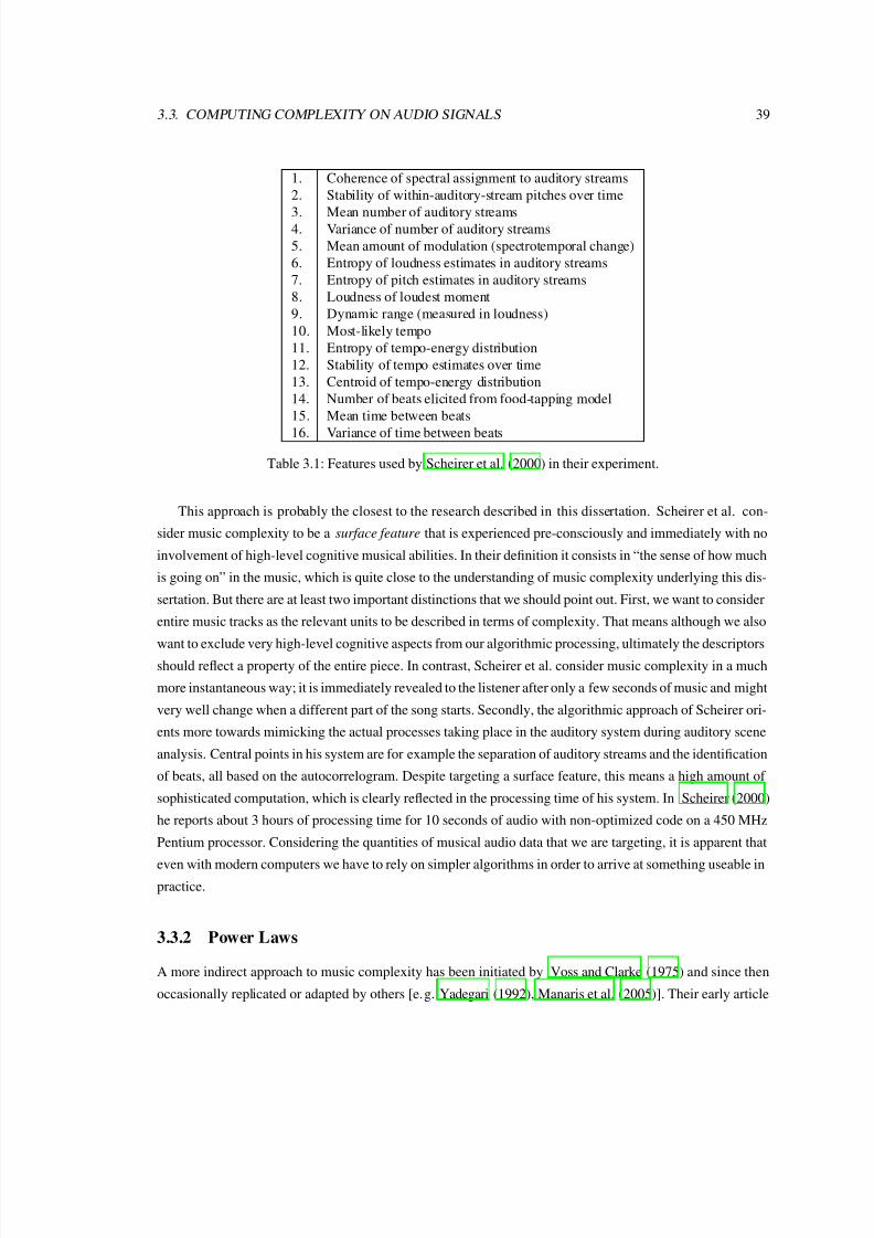
7/29/2019 Streich, S. (2007). Music Complexity. a Multi-faceted Description of Audio Content. Universitat Pompeu Fabra.
http://slidepdf.com/reader/full/streich-s-2007-music-complexity-a-multi-faceted-description-of-audio 56/124
3.3. COMPUTING COMPLEXITY ON AUDIO SIGNALS 39
1. Coherence of spectral assignment to auditory streams
2. Stability of within-auditory-stream pitches over time
3. Mean number of auditory streams4. Variance of number of auditory streams
5. Mean amount of modulation (spectrotemporal change)
6. Entropy of loudness estimates in auditory streams
7. Entropy of pitch estimates in auditory streams
8. Loudness of loudest moment
9. Dynamic range (measured in loudness)
10. Most-likely tempo
11. Entropy of tempo-energy distribution
12. Stability of tempo estimates over time
13. Centroid of tempo-energy distribution
14. Number of beats elicited from food-tapping model
15. Mean time between beats
16. Variance of time between beats
Table 3.1: Features used by Scheirer et al. (2000) in their experiment.
This approach is probably the closest to the research described in this dissertation. Scheirer et al. con-
sider music complexity to be a surface feature that is experienced pre-consciously and immediately with no
involvement of high-level cognitive musical abilities. In their definition it consists in “the sense of how much
is going on” in the music, which is quite close to the understanding of music complexity underlying this dis-
sertation. But there are at least two important distinctions that we should point out. First, we want to consider
entire music tracks as the relevant units to be described in terms of complexity. That means although we also
want to exclude very high-level cognitive aspects from our algorithmic processing, ultimately the descriptorsshould reflect a property of the entire piece. In contrast, Scheirer et al. consider music complexity in a much
more instantaneous way; it is immediately revealed to the listener after only a few seconds of music and might
very well change when a different part of the song starts. Secondly, the algorithmic approach of Scheirer ori-
ents more towards mimicking the actual processes taking place in the auditory system during auditory scene
analysis. Central points in his system are for example the separation of auditory streams and the identification
of beats, all based on the autocorrelogram. Despite targeting a surface feature, this means a high amount of
sophisticated computation, which is clearly reflected in the processing time of his system. In Scheirer (2000)
he reports about 3 hours of processing time for 10 seconds of audio with non-optimized code on a 450 MHz
Pentium processor. Considering the quantities of musical audio data that we are targeting, it is apparent that
even with modern computers we have to rely on simpler algorithms in order to arrive at something useable inpractice.
3.3.2 Power Laws
A more indirect approach to music complexity has been initiated by Voss and Clarke (1975) and since then
occasionally replicated or adapted by others [e.g. Yadegari (1992), Manaris et al. (2005)]. Their early article
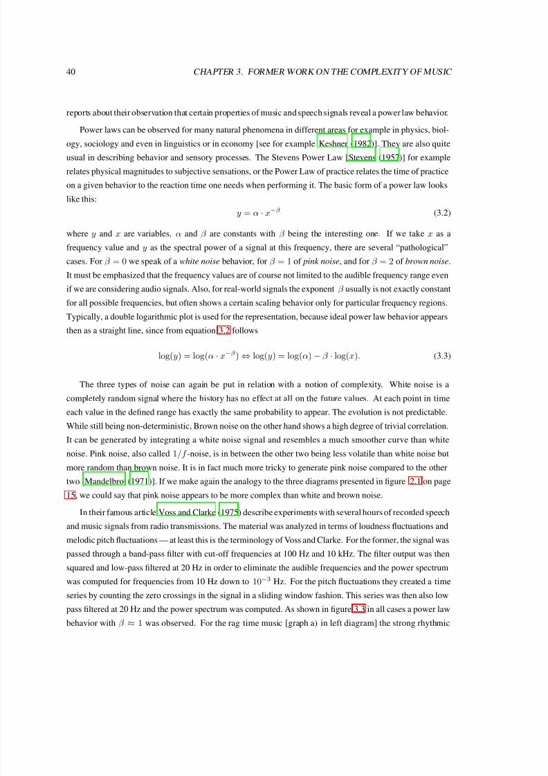
7/29/2019 Streich, S. (2007). Music Complexity. a Multi-faceted Description of Audio Content. Universitat Pompeu Fabra.
http://slidepdf.com/reader/full/streich-s-2007-music-complexity-a-multi-faceted-description-of-audio 57/124
40 CHAPTER 3. FORMER WORK ON THE COMPLEXITY OF MUSIC
reports about their observation that certain properties of music and speech signals reveal a power law behavior.
Power laws can be observed for many natural phenomena in different areas for example in physics, biol-
ogy, sociology and even in linguistics or in economy [see for example Keshner (1982)]. They are also quite
usual in describing behavior and sensory processes. The Stevens Power Law [Stevens (1957)] for example
relates physical magnitudes to subjective sensations, or the Power Law of practice relates the time of practice
on a given behavior to the reaction time one needs when performing it. The basic form of a power law looks
like this:
y = α · x−β (3.2)
where y and x are variables, α and β are constants with β being the interesting one. If we take x as a
frequency value and y as the spectral power of a signal at this frequency, there are several “pathological”
cases. For β = 0 we speak of a white noise behavior, for β = 1 of pink noise, and for β = 2 of brown noise.
It must be emphasized that the frequency values are of course not limited to the audible frequency range even
if we are considering audio signals. Also, for real-world signals the exponent β usually is not exactly constant
for all possible frequencies, but often shows a certain scaling behavior only for particular frequency regions.
Typically, a double logarithmic plot is used for the representation, because ideal power law behavior appears
then as a straight line, since from equation 3.2 follows
log(y) = log(α · x−β) ⇔ log(y) = log(α) − β · log(x). (3.3)
The three types of noise can again be put in relation with a notion of complexity. White noise is a
completely random signal where the history has no effect at all on the future values. At each point in time
each value in the defined range has exactly the same probability to appear. The evolution is not predictable.
While still being non-deterministic, Brown noise on the other hand shows a high degree of trivial correlation.
It can be generated by integrating a white noise signal and resembles a much smoother curve than white
noise. Pink noise, also called 1/f -noise, is in between the other two being less volatile than white noise but
more random than brown noise. It is in fact much more tricky to generate pink noise compared to the other
two [Mandelbrot (1971)]. If we make again the analogy to the three diagrams presented in figure 2.1 on page
15, we could say that pink noise appears to be more complex than white and brown noise.
In their famous article Voss and Clarke (1975) describe experiments with several hours of recorded speech
and music signals from radio transmissions. The material was analyzed in terms of loudness fluctuations and
melodic pitch fluctuations — at least this is the terminology of Voss and Clarke. For the former, the signal waspassed through a band-pass filter with cut-off frequencies at 100 Hz and 10 kHz. The filter output was then
squared and low-pass filtered at 20 Hz in order to eliminate the audible frequencies and the power spectrum
was computed for frequencies from 10 Hz down to 10−3 Hz. For the pitch fluctuations they created a time
series by counting the zero crossings in the signal in a sliding window fashion. This series was then also low
pass filtered at 20 Hz and the power spectrum was computed. As shown in figure 3.3 in all cases a power law
behavior with β ≈ 1 was observed. For the rag time music [graph a) in left diagram] the strong rhythmic

7/29/2019 Streich, S. (2007). Music Complexity. a Multi-faceted Description of Audio Content. Universitat Pompeu Fabra.
http://slidepdf.com/reader/full/streich-s-2007-music-complexity-a-multi-faceted-description-of-audio 58/124
3.3. COMPUTING COMPLEXITY ON AUDIO SIGNALS 41
Figure 3.3: Plots from Voss and Clarke (1975). Left: log10(loudness fluctuation) against log10(f ) for
a) Scott Joplin piano rags, b) Classical radio station, c) Rock station, d) News and talk station; Right:
log10(pitch fluctuation) against log10(f ) for a) Classical radio station, b) Jazz and Blues station, c) Rock
station, d) News and talk station.
organization is reflected in the deviations from the linear trend in the range of 1–10 Hz.
In another article Voss and Clarke (1978) report about a second experiment that builds up on their former
findings. They generated stochastic compositions where the note durations and the pitches were controlled by
independent white, pink, or brown noise generators3. Voss and Clarke played these musical pieces to several
hundred people including professional musicians and composers as well as musical laymen. To their ownsurprise the listeners very clearly preferred the music with 1/f and found it to be the most interesting among
the different versions. In the words of Voss and Clarke (1978):
The music obtained by this method was judged by most listeners to be much more pleasing than
that obtained using either a white noise source (which produced music that was “too random”) or
a 1/f 2 noise source (which produced music that was “too correlated”). Indeed the sophistication
of this “1/f music” (which was “just right”) extends far beyond what one might expect from
such a simple algorithm, suggesting that a “1/f noise” (perhaps that in nerve membranes?) may
have an essential role in the creative process.
Several other researchers conducted similar experiments as Voss and Clarke following their publication.Especially an other form of this 1/f behavior has been exploited, known as Zipf’s law [Zipf (1949)]. It is a
distribution law where the variable y of equation 3.2 corresponds to the frequency of occurrence of an event
and x corresponds to the position of the event in an ordered list for example according to size or –again– -
frequency of occurrence. The exponent β should be close to 1 in the ideal case. In Manaris et al. (2005) for
3The output of the noise generators was quantized and scaled in order to trigger the selection from limited sets of note durations and
pitches.

7/29/2019 Streich, S. (2007). Music Complexity. a Multi-faceted Description of Audio Content. Universitat Pompeu Fabra.
http://slidepdf.com/reader/full/streich-s-2007-music-complexity-a-multi-faceted-description-of-audio 59/124
42 CHAPTER 3. FORMER WORK ON THE COMPLEXITY OF MUSIC
example this idea has been applied to music (in the symbolic domain) by establishing a set of metrics that
examine the degree to which Zipf’s law is followed. As Manaris et al. report, they can be used successfully
in order to perform artist classification and to predict human pleasantness judgments.
While all these findings are very interesting and certainly have relevance for music information retrieval
applications, the connection to music complexity is a rather abstract one. Although the complexity assignment
we did for the three noise types is somehow reasonable and is frequently found in the literature, it remains a
rather analytical one and a relationship to properties of human perception is not obvious.
3.3.3 Detrended Fluctuation Analysis
Recently, Jennings et al. (2004) published an article on musical genre classification based on a feature that has
not been used before in the music information retrieval domain. What makes this article stand out especially
is the fact that the authors used exclusively this one feature only instead of combinations with more common
ones. They refer to it as the “Detrended Variance Fluctuation Exponent”, since it originates from a technique
called “Detrended Fluctuation Analysis” (DFA). The technique was introduced by Peng et al. (1994) and
is intended for the analysis of chaotic time series. It was first applied by Peng in a biomedical context on
nucleotide and heartbeat rate time series. Other applications include financial time series [as reported in
Ausloos (2000)]. The method is related to the power law analysis we just discussed in section 3.3.2 in the
sense that it can also reveal correlation properties of white, pink, or brown noise in a time series. It has the
special quality that it works well for non-stationary data.
The method intends to identify the scaling behaviour of a time series. This is best explained by consid-
ering an unbounded time series (i. e. with no upper limit for its values). If we plot a portion of such a series
over the time axis, we will need a certain range r1 of values on the y-axis in order to visualize all the elements
falling into the temporal segment τ 1. Imagine now that we are zooming in on the plot. This zoom can be
expressed as a factor on each axis, for example we can say that the new portion has 0.5 times the length of
the previous one, such that τ 2 = τ 1/2. In this case we can expect that the range of values on the y-axis has
changed as well, from r1 to r2. By taking the quotientlog(r1/r2)log(τ 1/τ 2)
we obtain a scaling exponent α. This expo-
nent can be calculated for different time scales (i. e. for different values of τ 1 and τ 2). If we systematically
increase or decrease the time scales and for each step calculate the scaling exponent, we obtain a function
α(τ ). From this function we can get an insight into the scaling properties of the time series. For example
the scaling can be stable (constant level of α) or it might expose irregularities. Also the general level of α
is significant. For a pure white noise signal it is 0.5, for pink noise it is 1.0, and for brown noise it is 1.5. αlevels below 0.5 indicate that the signal is anti-correlated [Matassini (2001) pp. 41–43].
However original the descriptor of Jennings et al. (2004) might be, it is not obvious on the first gaze
how it reflects semantic concepts of music that a listener can relate to. Since their paper focusses on the
performance in genre classification, this aspect was not directly considered, because mainly the output of
the classifier was of interest. But they state that the strong periodic trends in dance music styles like Techno
or Brazilian Forro) make it easily distinguishable in terms of the DFA exponent from high art music such as

7/29/2019 Streich, S. (2007). Music Complexity. a Multi-faceted Description of Audio Content. Universitat Pompeu Fabra.
http://slidepdf.com/reader/full/streich-s-2007-music-complexity-a-multi-faceted-description-of-audio 60/124
3.3. COMPUTING COMPLEXITY ON AUDIO SIGNALS 43
Figure 3.4: Average DFA exponent α for different music genres [from Jennings et al. (2004)]
Javanese Gamelan, Hindustani, or Western European Classical Tradition (WECT). The average α value of the
ten tracks from each genre is clearly lower for the former as can be seen in figure 3.4. “Jazz, Rock and Roll,
and Brazilian popular music may occupy an intermediary position between high art music and dance music:
complex enough to listen to, but periodic enough to dance to,” Jennings et al. (2004) speculate. Hence, we
could think of this feature as a measure of “danceability”, which certainly is an aspect of rhythmic complexity
that is immediately accessible for human music perception. A very appealing property of the DFA method
for our needs is also that it can be applied directly to the audio file and does not rely on the extraction of other
descriptors like onsets or beats as a preprocessing step. An adaptation of the algorithm with further details
will be described in section 4.5.1 of the next chapter.
3.3.4 Conclusion
To conclude we can state that the matter of music complexity estimation from audio signals has not been
studied to a great extent so far. Although we reviewed different approaches of this kind, it has to be noticed
that they either fall short of practicality for our context or have not been fully exploited yet in terms of their
usefulness for MIR applications. It has therefore been a goal of this dissertation to contribute with original
ideas and with adaptations of existing work to make music complexity better accessible for the current topics
of audio-based music information retrieval.

7/29/2019 Streich, S. (2007). Music Complexity. a Multi-faceted Description of Audio Content. Universitat Pompeu Fabra.
http://slidepdf.com/reader/full/streich-s-2007-music-complexity-a-multi-faceted-description-of-audio 61/124
44 CHAPTER 3. FORMER WORK ON THE COMPLEXITY OF MUSIC

7/29/2019 Streich, S. (2007). Music Complexity. a Multi-faceted Description of Audio Content. Universitat Pompeu Fabra.
http://slidepdf.com/reader/full/streich-s-2007-music-complexity-a-multi-faceted-description-of-audio 62/124
Chapter 4
Complexity Facets and their
Implementation
In this chapter we will review in detail the algorithms that have been developed by the author in the course
of this dissertation. For each algorithm we will first explain the general idea behind it and then present the
actual implementation.
4.1 Working on Facets
As we said in section 1.2 already, we want to address music complexity in different facets. Why should
this be done? Didn’t we say that for complexity “the whole is more than the sum of its parts”? It is true,
but nevertheless there are good reasons to split the work up. A subdivision of music into separate facets is
a common practice in musical analysis. The divide and conquer strategy is widespread in many fields of
science. Our target of a naıve listener on the other hand is not speaking in direct favor of such separation.
Such a listener should not be assumed to analyze the mentioned facets independently in order to arrive at
his judgement of complexity. But it is not our goal to mimic the process of obtaining a judgement of the
musical complexity. Our interest is rather that the final result of such a process is predicted correctly by the
algorithms. We can therefore look for a way that gives us the least trouble instead of trying to follow closely
every link in the human music processing chain.With respect to music complexity, in Finnas (1989) we find the statement that “unusual harmonies and
timbres, irregular tempi and rhythms, unexpected tone sequences and variations in volume” raise the level
of perceived complexity in music. We can see that the facets of music (harmony, rhythm, volume, . . . )
mentioned by Finnas are at least partly independent from each other. For example one music track can
contain very sophisticated rhythm patterns, but no melodic voice at all. Another one might have unexpected
changes in volume and timbre, but very straightforward melody and chord sequences. Which one should
45

7/29/2019 Streich, S. (2007). Music Complexity. a Multi-faceted Description of Audio Content. Universitat Pompeu Fabra.
http://slidepdf.com/reader/full/streich-s-2007-music-complexity-a-multi-faceted-description-of-audio 63/124
46 CHAPTER 4. COMPLEXITY FACETS AND THEIR IMPLEMENTATION
be rated more complex in a direct comparison? Looking at the problem this way calls for a multi-faceted
approach with an individual complexity estimation for each facet. A joint measure of global complexity does
not necessarily make sense under these circumstances. The separation of facets also gives us the opportunity
to account up to a certain degree for the subjectivity that has been mentioned in chapter 2. If different people
consider the different facets to be of different importance, then they can assign weights to them according
to their personal preference, while the single values still remain objectively comparable for any user of the
descriptors. Finally, the break down into facets is also a matter of practicality in terms of algorithm design.
A holistic model that computes a single, overall complexity value without individual analysis of the different
musical aspects would be much more difficult to build and to test. We therefore deal with music complexity
individually in the facets described below.
4.2 Acoustic Complexities
Under Acoustic Complexity we want to capture two different aspects of a musical audio track: the dynamic
and the spatial properties. The former are related to the loudness evolution throughout a musical recording,
while the latter correspond to the rendering of the auditory scene. From these explanations it is clear al-
ready that acoustic complexity is not completely intrinsic to the music, but rather to the recording and the
performance. Nevertheless, we found it worthwhile to include this complexity facet, because digital music
tracks only exist as recorded performances1 of music. So it is not possible to listen to one without noticing
characteristics of the other.
The dynamic complexity component relates to the properties of the loudness evolution within a musical
track. We refer to it in terms of abruptness and rate of changes in dynamic level. Also the dynamic range has
to be considered here, since a sudden jump by 6dB will be considered more surprising than one by only 1dB.
A major design decision for the complexity model is the definition of the time scope. By keeping the frame
size small one can find the distinction between dynamically compressed and uncompressed material. The
former has less rapid changes in loudness than the latter and can therefore be considered less complex. As we
will see later in this chapter, there is some overlap with the rhythmic complexity descriptor here. With longer
windows one detects fades and dynamic changes between larger segments, for example a very soft passage
embedded between two rather loud ones. By looking at this time scope we can for example distinguish
between music in the classical style, which often uses a wide range of loudness levels within one piece, and
mainstream popular music that has been made to fit modern radio broadcasting by keeping continuously a
very high loudness level throughout the entire track.
For the spatial complexity component we consider only stereo recordings and no advanced multi-channel
formats for the time being. Currently, two channel stereo tracks form by far the majority of items in digital
music file databases, whereas 5.1 recordings, for example, are still very rare. A straight-forward example
for spatial complexity thus is the disparity of the stereo channels. A quasi mono situation with the same
1For electronic music the concepts of “recording” and “performing” have to be understood in a slightly wider sense here.

7/29/2019 Streich, S. (2007). Music Complexity. a Multi-faceted Description of Audio Content. Universitat Pompeu Fabra.
http://slidepdf.com/reader/full/streich-s-2007-music-complexity-a-multi-faceted-description-of-audio 64/124
4.2. ACOUSTIC COMPLEXITIES 47
signal in both channels reveals less complexity than a recording that has only little correlation between the
two channels. But also more advanced aspects are to be considered, such as the movement of the acoustical
center of effect within the stereo image, and sound effects changing the spatial impression (e. g. delay and
reverberation effects). In simpler words we could say that spatial complexity should be a measure of the
wideness and the amount of fluctuation in the stereo image. As with the dynamic component already, spatial
complexity again depends to a great extent on the quality of the recording.
4.2.1 Implementation of the Dynamic Component
The first step towards dynamic complexity computation is the calculation of an accurate estimate of the
perceived loudness. Psychoacoustics are a well studied field and quite reliable measures exist in the literature
for loudness estimation of isolated sounds, like sinusoids or noise [Zwicker and Fastl (1990), Moore et al.(1997)]. For the complex sounds that form a musical performance however accurate loudness estimation is
a very complicated task. Not only temporal and spectral masking have an influence here, but also subjective
components play a role [Skovenborg and Nielsen (2004)]. Finally, the playback level of a digital track cannot
be known, so we can only achieve an estimation of the loudness level relative to an arbitrary reference. For
our needs it is also important to keep computational efficiency in mind, since the goal is to be able to use the
descriptors on large collections of music tracks. We therefore want to pay more attention to a simple and fast
approximation than to a very sophisticated and more accurate procedure.
In the course of this dissertation two different implementations for dynamic complexity have been devel-
oped. The first one was chosen, because of its easy implementation. It is operative in the time domain and
utilizes a simplified loudness model as described in Vickers (2001). Some modifications and additions have
been made in order to make the algorithm fit for the desired task. The second one uses a slightly more sophis-
ticated approach based on Pampalk’s implementation of Stevens’ method [Stevens (1956), Stevens (1961)]
including a modified version of the outer ear filter from Terhardt’s pitch perception model [Terhardt (1979)].
This implementation has the advantage that the computed intermediate results can also be used for the timbre
complexity estimation (see section 4.3.1).
Implementation using Vickers’ loudness estimation
As a first step the algorithm applies a very simplified “B” weighting function to the audio signal in order to
account for the human ear’s transfer function. For efficiency reasons this weighting is done by a first-order
Butterworth high-pass filter with a cut-off frequency of 200 Hz. So actually only the low end of the weighting
function is approximated. In the case of music signals this is tolerable, since they have much more energy in
the bass and mid-range compared to the high frequencies.
The pre-emphasized signal x pre(n) is then fed into a root-mean-square level detector with an integrated
smoothing function. This level detector consists of a running average V ms (eq. 4.1) that is downsampled
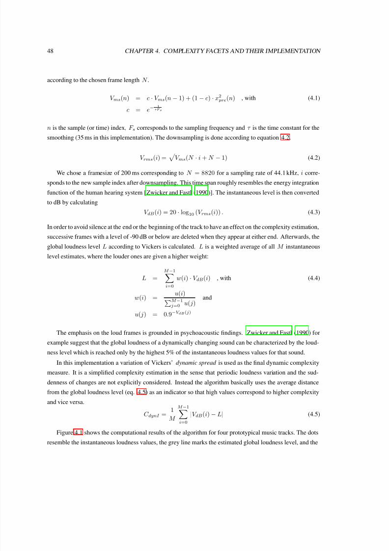
7/29/2019 Streich, S. (2007). Music Complexity. a Multi-faceted Description of Audio Content. Universitat Pompeu Fabra.
http://slidepdf.com/reader/full/streich-s-2007-music-complexity-a-multi-faceted-description-of-audio 65/124
48 CHAPTER 4. COMPLEXITY FACETS AND THEIR IMPLEMENTATION
according to the chosen frame length N .
V ms(n) = c · V ms(n − 1) + (1 − c) · x2 pre(n) , with (4.1)
c = e−1
τF s
n is the sample (or time) index, F s corresponds to the sampling frequency and τ is the time constant for the
smoothing (35 ms in this implementation). The downsampling is done according to equation 4.2.
V rms(i) =
V ms(N · i + N − 1) (4.2)
We chose a framesize of 200 ms corresponding to N = 8820 for a sampling rate of 44.1 kHz, i corre-
sponds to the new sample index after downsampling. This time span roughly resembles the energy integration
function of the human hearing system [Zwicker and Fastl (1990)]. The instantaneous level is then convertedto dB by calculating
V dB(i) = 20 · log10 (V rms(i)) . (4.3)
In order to avoid silence at the end or the beginning of the track to have an effect on the complexity estimation,
successive frames with a level of -90 dB or below are deleted when they appear at either end. Afterwards, the
global loudness level L according to Vickers is calculated. L is a weighted average of all M instantaneous
level estimates, where the louder ones are given a higher weight:
L =
M −1
i=0
w(i) · V dB(i) , with (4.4)
w(i) =u(i)M −1j=0 u( j)
and
u( j) = 0.9−V dB(j)
The emphasis on the loud frames is grounded in psychoacoustic findings. Zwicker and Fastl (1990) for
example suggest that the global loudness of a dynamically changing sound can be characterized by the loud-
ness level which is reached only by the highest 5% of the instantaneous loudness values for that sound.
In this implementation a variation of Vickers’ dynamic spread is used as the final dynamic complexity
measure. It is a simplified complexity estimation in the sense that periodic loudness variation and the sud-
denness of changes are not explicitly considered. Instead the algorithm basically uses the average distance
from the global loudness level (eq. 4.5) as an indicator so that high values correspond to higher complexity
and vice versa.
C dynI =1
M
M −1i=0
|V dB(i) − L| (4.5)
Figure 4.1 shows the computational results of the algorithm for four prototypical music tracks. The dots
resemble the instantaneous loudness values, the grey line marks the estimated global loudness level, and the

7/29/2019 Streich, S. (2007). Music Complexity. a Multi-faceted Description of Audio Content. Universitat Pompeu Fabra.
http://slidepdf.com/reader/full/streich-s-2007-music-complexity-a-multi-faceted-description-of-audio 66/124
4.2. ACOUSTIC COMPLEXITIES 49
0 20 40 60 80 100 120 140 160 180−60
−50
−40
−30
−20
−10
L o u d n e s s i n d B
a) Heavy Metal
0 20 40 60 80 100 120 140 160 180 200−60
−50
−40
−30
−20
−10
L o u d n e s s i n d B
b) Pop Song
0 20 40 60 80 100 120 140 160 180 200−60
−50
−40−30
−20
−10
L o u d n e s s
i n d B
c) Jazz Guitar Solo
0 40 80 120 160 200 240−60
−50
−40
−30
−20
−10
time in s
L o u
d n e s s i n d B
d) Classical Symphony
Figure 4.1: Instantaneous loudness as in eq. 4.3 (dots), global loudness as in eq. 4.4 (grey solid line), and
average distance margin as in eq. 4.5 (dashed lines) for four example tracks.

7/29/2019 Streich, S. (2007). Music Complexity. a Multi-faceted Description of Audio Content. Universitat Pompeu Fabra.
http://slidepdf.com/reader/full/streich-s-2007-music-complexity-a-multi-faceted-description-of-audio 67/124
50 CHAPTER 4. COMPLEXITY FACETS AND THEIR IMPLEMENTATION
dashed lines indicates the average distance margin. In figure 4.1 a we see a highly saturated heavy metal track
with a basically flat dynamic level. The global loudness was estimated as -14.9 dB and the average deviation
C dynI from this level is only 1.37 dB. Figure 4.1 d shows another extreme, a recording of classical music
that changes in loudness between -50 dB and -20 dB. The algorithm estimates a clearly lower global loudness
of -24.8 dB and an average deviation of 8.05 dB. In between there is a pop song (figure 4.1 b) moderately
varying in loudness with a global level of -16.4 dB and an average deviation of 3.71 dB. The jazz guitar solo
from figure 4.1 c is recorded at very low volume. The estimated global loudness is only -25 dB. Despite some
singular drops down to -50 dB due to short pauses between played notes, the average deviation amounts only
to 4.5 dB and is thus considerably smaller than that of the classical recording.
Implementation based on Pampalk’s approach
Alternatively, an implementation based on the ma sone function of Pampalk’s MA Toolbox2
has been done.Apart from allowing for a more accurate loudness estimation, the reason for this is also that the preprocessing
is similar to the one used for the timbre complexity computation we will discuss in section 4.3. Despite
the more expensive processing steps, this way is therefore computationally more efficient if both descriptors
(dynamic complexity and timbre complexity) are to be computed for the same track.
The processing starts by breaking the input signal down into overlapping frames of roughly 16 ms length.
We use a Hann window (eq. 4.6) for weighting the samples x(n) within each frame in order to avoid edge
effects of the Fourier Transform. The overlap factor is 0.5 giving us a relatively high temporal resolution of
8ms.
w(n) = 0.5 · 1 − cos(2πn
N − 1) , with 0 ≤ n < N (4.6)
After a frame is transformed into the frequency domain via the Fast Fourier Transform, the normalized power
spectrum P (k) is computed:
P (k) =
2 · X (k)N −1n=0 w(n)
2
(4.7)
where
X (k) =
N −1n=0
x(n) · w(n) · e−2πjN kn , with 0 ≤ k ≤
N
2.3 (4.8)
The power spectrum is then weighted with a curve that is inspired by the frequency response of the outer ear.
As can be seen in figure 4.2 the modified version we use is more balanced and gives a milder emphasis on
the frequency region between 2 kHz and 5 kHz than Terhardt’s original curve [ Terhardt (1979)] that is also
depicted. The curve assigns a weight A(f ) to each frequency value f (measured in kHz) according to the
following formula:
A(f ) = 10
0.5·e−0.6·(f −3.3)2−5·f 4·10−5−2.184·f −0.8
. (4.9)
2http://www.ofai.at/ elias.pampalk/ma/index.html3Since we only deal with real valued input signals, the values for N
2< k < N are redundant and therefore omitted in the further
processing steps.

7/29/2019 Streich, S. (2007). Music Complexity. a Multi-faceted Description of Audio Content. Universitat Pompeu Fabra.
http://slidepdf.com/reader/full/streich-s-2007-music-complexity-a-multi-faceted-description-of-audio 68/124
4.2. ACOUSTIC COMPLEXITIES 51
0 2 4 6 8 10 12 14 16 18 200
0.2
0.4
0.6
0.8
1
1.2
1.4
1.6
frequency in kHz
w e i g h t
original Terhardt weightingmodified Terhardt weighting
Figure 4.2: Frequency weighting curves for the outer ear.
Evaluating equation 4.9 only at the center frequencies of the bins from the discrete Fourier spectrum we
obtained from equation 4.8, we can create an array of weight values A(k). The weighting of the power
spectrum itself can then be described by the simple multiplication:
P w(k) = P (k) · A(k)2. (4.10)
From this weighted power spectrum we compute then the bark band energies P cb(l) by summing up the
values of P w(k) falling in between the lower bound lowB(l) and the upper bound highB(l) of each of the
24 bark bands as defined in Zwicker and Fastl (1990):
P cb(l) =
highB(l)
k=lowB(l)
P w(k) (4.11)
Once the bark band energies are computed, a heuristic spreading function s(l) following Schroeder et al.
(1979) is applied to account for spectral masking effects in human sound perception. Temporal masking
effects, that also exist in human perception are not accounted for at this point. The spreading is realized by
convoluting the bark band energies P cb(l) with the spreading function
s(l) = 10(0.75·l+1.937−1.75·√ l2+0.948·l+1.225) (4.12)

7/29/2019 Streich, S. (2007). Music Complexity. a Multi-faceted Description of Audio Content. Universitat Pompeu Fabra.
http://slidepdf.com/reader/full/streich-s-2007-music-complexity-a-multi-faceted-description-of-audio 69/124
52 CHAPTER 4. COMPLEXITY FACETS AND THEIR IMPLEMENTATION
resulting in the spread energy distribution
P spread(m) =24l=1
P cb(l) · s(m − l) , with 1 ≤ m ≤ 24. (4.13)
We then limit the lower bound of the obtained band energies to 1 in order to avoid numerical problems with
the following conversion to decibel scale, which is given by
P dB(m) = 10 · log10(P spread(m)). (4.14)
The total instantaneous loudness is then estimated following the method described in Stevens (1956) and
Stevens (1961) for the case of third octave bands. To do so we first need to convert the energy values of
each band from the decibel scale to the sone scale. The sone scale was proposed by Stevens (1957) to
provide a linear correspondence to human loudness perception (i. e. if a sound has twice as much sones as
a reference sound, then it is also perceived as being twice as loud). Pampalk’s implementation is not 100%
accurate at this point, since the decibel values would need to be converted into phons first [as described in
Bladon and Lindblom (1981)]. This is a non-linear operation, which would make it necessary to quantize
the values according to equal loudness curves obtained from a voluminous lookup table or through a set of
heuristic approximations. For simplicity, we use the conversion formula directly on the band energy values,
considering that the sound sensitivity of the human ear at different frequencies has been accounted for already
partly in equation 4.9:
L(m) = 20.1·(P dB(m)−40) for P dB(m) ≥ 40 (4.15)
(P dB(m) − 40)2.642 else. (4.16)
Finally, we arrive at the total loudness estimate for each frame by evaluating
Ltotal = 0.85 · L(mmax) + 0.15 ·24i=1
L(i), (4.17)
where mmax is the index of the band with the biggest loudness in the frame. Before proceeding with the
complexity estimation it is first necessary to smoothen the loudness evolution, since so far we have been
considering only isolated frames representing 16 ms excerpts. As with Vickers’ method, we again apply an
exponential decay function in a sliding window fashion exactly as shown in equation 4.1, but with a time
constant corresponding to 800 ms or 100 overlapped frames. This value was empirically found and results
from the aim to reduce the influence of loud, but regular percussion events in front of a lower overall loudness
level. In a second smoothing step we are then calculating the running average over 200 consecutive values,
corresponding to 1.6 s. We decimate the sequence to a resolution of 2.5 values per second by computing this
operation only for every 50th value.

7/29/2019 Streich, S. (2007). Music Complexity. a Multi-faceted Description of Audio Content. Universitat Pompeu Fabra.
http://slidepdf.com/reader/full/streich-s-2007-music-complexity-a-multi-faceted-description-of-audio 70/124
4.2. ACOUSTIC COMPLEXITIES 53
As we are not estimating a global loudness level for the entire track, this time the complexity estimation
is calculated slightly different. We consider the average fluctuation of successive loudness values as the
complexity indicator. So it is now more the suddenness and the amount of loudness changes, that determine
the complexity, while with the approach following Vickers the focus was more one the duration and distance
away from the global loudness level of the track. It was found advantageous to move back to the decibel
level again before evaluating the complexity measure, so with Ltotsd(n) being the smoothed, decimated total
loudness values we obtain:
C dynII =1
N − 1
N −1n=1
|log10(Ltotsd(n)) − log10(Ltotsd(n + 1))| , (4.18)
with N being the number of decimated loudness values for the entire track. The use of the logarithm in this
equation actually means that we are looking at loudness fluctuation in terms of ratios on the sone scale ratherthan in terms of absolute deviations. This makes sense, because a jump that doubles the perceived loudness
will (at least ideally) always result in a ratio of 1:2 no matter at which level it starts.
Figure 4.3 shows the resulting loudness curves for the four example tracks we already saw in figure
4.1. Again, the heavy metal track depicted in figure 4.3 a shows a very flat loudness curve over time. The
complexity in terms of the average absolute difference between consecutive values (eq. 4.18) is therefore
quite low and amounts only to 0.134. Looking at figure 4.3 b, the pop song, we can observe the stronger
smoothing compared to the method based on Vickers’ algorithm. There is much less fluctuation visible than
in the instantaneous loudness in figure 4.1 b. Still, the complexity is clearly higher than for the heavy metal
track with C dynII = 0.247. In figure 4.3 c, the jazz guitar piece, the effect of the smoothing is even more
visible. The short sudden drops in loudness have been averaged out, but compared to the pop song there is
clearly a higher amount of fluctuation in the signal. This is also reflected in the complexity value, which
reaches 0.304 for this track. Finally, for figure 4.3 d we see again the strong changes in the loudness level,
which are typical for many recordings of classical music. This track yields again the highest complexity with
a value of 0.488.
4.2.2 Implementation of the Spatial Component
The spatial component of acoustic complexity estimation is, as we said, mainly focusing on the disparity of
the stereo channels and the amount of fluctuation in the stereo image. While methods exist to calculate the po-sition of a single sound source in space when it is recorded by an array of microphones [e. g. Silverman et al.
(2005)], the identification of the center of effect in the stereo panorama is a somewhat different problem.
Since usually complex mixtures of sounds are involved in each channel, some kind of source separation tech-
nique would be needed in order to obtain very accurate results. However, this type of auditory scene analysis
usually involves very heavy processing and the quality of the separation can vary a lot with different types of
input signals and an unknown number of mixed sources.

7/29/2019 Streich, S. (2007). Music Complexity. a Multi-faceted Description of Audio Content. Universitat Pompeu Fabra.
http://slidepdf.com/reader/full/streich-s-2007-music-complexity-a-multi-faceted-description-of-audio 71/124
54 CHAPTER 4. COMPLEXITY FACETS AND THEIR IMPLEMENTATION
50 100 150 200 250 300
10
20
30a) Heavy Metal
L o u d n e s s
50 100 150 200 250 300 350
10
20
30
L o u d n e
s s
c) Jazz Guitar Solo
50 100 150 200 250 300 350 400
10
20
30
frame index
L o u d n e s s
d) Classical Symphony
50 100 150 200 250 300 350
10
20
30
L o u d n e s s
b) Pop Song
Figure 4.3: Instantaneous total loudness values (eq. 4.17) on logarithmic scale for the same four tracks shownin figure 4.1.
A work-around for this bottleneck can be found in methods that are commonly used in room acoustic
measurements to quantify the reverberation or the spaciousness of an acoustic environment. Although we
cannot hope to find the wideness or the amount of fluctuation in the stereo image directly being reflected
in these measures, we might at least obtain a rough estimation of the “size” of the auditory scene. A good
overview over several methods in use can be found in Griesinger (1999). Usually, these measures take the
room impulse response as their input and are thus not suited for a continuous signal as music. An exception
is the InterAural Difference (IAD) introduced by Griesinger, which, as he states, can also be computed as
a continuous function for music signals. It is computed according to equation 4.19, where L(t) and R(t)
refer to the audio signal in the left and the right channel, and the equalization eq consists of a low frequency
enhancement of 6dB per octave below 300Hz.
IAD(t) = 10 · log10
eq (L(t) − R(t))2
L(t)2 + R(t)2
(4.19)

7/29/2019 Streich, S. (2007). Music Complexity. a Multi-faceted Description of Audio Content. Universitat Pompeu Fabra.
http://slidepdf.com/reader/full/streich-s-2007-music-complexity-a-multi-faceted-description-of-audio 72/124
4.2. ACOUSTIC COMPLEXITIES 55
As a function of time, the IAD indicates the direction from which the main acoustical energy is coming. A
simple measure of complexity would therefore be the variance of IAD(t).
A slightly more sophisticated alternative accounting for stereo effects based on a delay between the chan-
nels involves the cross-correlation function CC R(τ ) =tendtstart
L(t) · R(t − τ ) between the channels, where
the lag τ should be evaluated within the boundaries of ±2 ms. Delays greater than 2 ms are not perceived
as a shift of the source in the stereo image anymore, but are identified as an echo. Often, the function is
normalized by the square root of the product of the sound energies in the two channels and then known as
the Inter Aural Cross-Correlation Coefficient (IACC). This function needs to be computed on short fragments
of the signal (e. g. tend − tstart = 80 ms), since the stereo image cannot be assumed to be stable over long
periods of time in a music recording. We would then need to identify the lag τ max that maximizes the cross-
correlation function for a given fragment. A measure of the spatial complexity could be seen in the variance
of τ max across all the fragments of the entire music track.It must be stated again that the originally intended use of these measures is somewhat different from our
needs. The measures are supposed to reveal information about the acoustic properties of a real room when an
impulse or a (dry) sound is played back inside. The two channels in equation 4.19 correspond to the signal
recorded by two microphones (e. g. inside an artificial head) in the room. We, on the contrary, already have
a stereo recording, which was produced with very different techniques, but we would simply have to treat
it as the recording of the dummy head in a “virtual” room. An extensive discussion of this problem and
some experimental results can be found in Mason (2002). It can basically be said, that this approach is only
successful when very special conditions apply to the recording (e. g. a solo instrument recorded with a stereo
room microphone). With very rich mixtures of sources and studio edited material the results become more
and more arbitrary.
Given these shortcomings we looked for a compromise between a very costly and difficult, complete
auditory scene analysis and the simple but inaccurate direct comparison of the stereo channels. The choice
fell on a method proposed in Barry et al. (2004) that has been further developed for human-assisted source
separation by Vinyes et al. (2006) at Pompeu Fabra University. The basic idea is to compare the short-time
Fourier spectra of the two stereo channels in order to identify the energy distribution in the stereo image
across the audible frequency range. While the actual separation of the sources based on this distribution still
requires human interaction or very advanced heuristics, for our needs this representation is already sufficient.
We can analyze the fluctuation in this distribution over time as a cue for the amount of changes in the auditory
scene. And we can also compute the sharpness or flatness of this distribution as an indicator for the width of
the stereo image. Strictly speaking, this method is only applicable with accuracy, in cases where the stereo
image is created through intensity differences between the channels and not through a temporal delay. As
intensity stereophony is the most common practice in studio production and even with a delay between the
channels there is often also an intensity difference, the method can be considered much more versatile in our
context than the afore-mentioned measures from room acoustics.
As mentioned, the basis for the processing is once more a segmentation of the audio signal into frames

7/29/2019 Streich, S. (2007). Music Complexity. a Multi-faceted Description of Audio Content. Universitat Pompeu Fabra.
http://slidepdf.com/reader/full/streich-s-2007-music-complexity-a-multi-faceted-description-of-audio 73/124
56 CHAPTER 4. COMPLEXITY FACETS AND THEIR IMPLEMENTATION
followed by the multiplication with a window function w(n) and a Fourier transformation (eq. 4.8 on page
50). The chosen frame length and overlap factor correspond this time to 93 ms and 0.5 respectively. In
contrast to the dynamic complexity processing, we are now obtaining pairs of values X L(k) and X R(k),
since we are processing the left and the right channel separately in a synchronized manner. Again we compute
the power spectra P L(k) = |X L(k)|2 and P R(k) = |X R(k)|2, this time without normalizing by the window
weight. For each of these pairs of values we estimate now the angle tan(α(k)) corresponding to the direction
of the acoustic energy source in a horizontal 180°range:
tan(α(k)) =P R(k) − P L(k)
2
P R(k) · P L(k)(4.20)
In a second step these values are quantized and converted with a reference table mapping them into the range
1 ≤ αq(k) ≤ 180, with αq(k) being a natural number. A value of 1 would thus refer to the acoustic energy
in the respective frequency bin being concentrated in the left channel only, for a value of 180 it would be
the right channel, and for the others something in between. Now we use this information to compute the
instantaneous energy distribution E spatial for each frame. First we obtain the instantaneous energies in the
individual frequency bins
E (k) = log10(P R(k)) + log10(P L(k)) + 14, (4.21)
where the constant 14 corresponds to an empirical offset used for noise suppression, since we limit the values
E (k) to a lower bound of zero before proceeding with the calculations. The energy distribution is then
obtained by summing all values E (k) of one frame that have the same value αq(k):
E spatial(m) =
k∈{k|αq(k)=m}E (k) , with 1 ≤ m ≤ 180. (4.22)
Figure 4.4 shows two snapshots of such distributions. In track one the stereo image is rather wide and there is
a lot of fluctuation. In the snapshot we can clearly see that, at that position in time, the left channel contains
overall much more energy and one source seems to be playing at roughly 40°to the left from the center. In
contrast, for track two, a historic jazz recording, there is a big peak in the center with more or less balanced
and relatively low wings on either side indicating an auditory image close to a mono recording. Before the
actual complexity is estimated, we apply several steps of cleaning and smoothing to reduce effects of noise
and inaccuracies in the calculation of the distributions. First the distribution of each frame i is normalized by
the total frame energy:
E [i]norm(m) =E
[i]spatial(m)
2048 +180k=1 E [i](k)
, with 1 ≤ m ≤ 180. (4.23)
The constant 2048 has two functions. First, it is a simple numerical trick to avoid the problem of dividing
by zero in the case of silent frames. Second, it gives additional emphasis to louder frames, since now we

7/29/2019 Streich, S. (2007). Music Complexity. a Multi-faceted Description of Audio Content. Universitat Pompeu Fabra.
http://slidepdf.com/reader/full/streich-s-2007-music-complexity-a-multi-faceted-description-of-audio 74/124
4.2. ACOUSTIC COMPLEXITIES 57
0 20 40 60 80 100 120 140 160 180
0
100
200
300
400
500
600
700
800
900
αq
E n e r g y
track1track2
Figure 4.4: Snapshots of energy distributions on 180°horizontal plane for two example tracks (track1= mod-
ern electronic music, track2= historic jazz recording).
are assigning the weight g[i] =180m=1 E
[i]norm(m) to each frame i. The normalized distributions can be
represented in form of a matrix, where the first dimension refers to the angle αq and the second to the frame
index. To this matrix we apply now a 3x3 median filter that removes extreme outliers in the distribution.
Afterwards we use a box filter4 of size 7x11. That means for each element we are computing the average for
the neighborhood of ±3◦ and ±230 ms, which significantly reduces the details leaving only the major shifts
in the distribution.
Now we can readily apply the following formula to estimate the spatial fluctuation as an indicator for
complexity in terms of changes in the stereo image over time:
C spatFluc =1
N − 1
N −1i=1
g[i] · g[i+1] ·180j=1
E [i]norm( j) − E [i+1]norm( j)
, (4.24)
where N is the total number of frames of the track. While this measure is well suited to identify static images
from those that constantly change, it does not account for the wideness of the acoustical scene. Whether a
source is moving only several degrees away from the center or it changes from the extreme left to the extreme
right is not very well reflected despite it can be considered a relevant difference in terms of complexity.Also, two static images will yield the same score even though one might be a mono recording and the other
uses the entire available stereo panorama. For this reason the obtained energy distributions have been used
for a second complexity measure. As an auxiliary result we first compute the “center of mass” c[i]g of each
distribution. If we consider the distribution as a one-dimensional object with 180 partitions, where the weight
4A box filter is the equivalent to a moving average filter in two dimensions. In our case it smoothes simultaneously the temporal and
the directional evolution.

7/29/2019 Streich, S. (2007). Music Complexity. a Multi-faceted Description of Audio Content. Universitat Pompeu Fabra.
http://slidepdf.com/reader/full/streich-s-2007-music-complexity-a-multi-faceted-description-of-audio 75/124
58 CHAPTER 4. COMPLEXITY FACETS AND THEIR IMPLEMENTATION
of each partition is given by the corresponding energy E [i]norm(m), then we have
c[i]g =
180m=1 m · E [i]norm(m)
E [i]sum
, with E [i]sum =180m=1
E [i]norm(m). (4.25)
For numerical reasons we have to take care of the case E [i]sum = 0, which can occur for silent or extremely
soft frames. For these cases the centroid c[i]g will be set to the neutral position, which is 90. Likewise, in the
following processing we will replace the corresponding values of E [i]sum with the equivalent to ∞. We now
define the second complexity measure as the average spatial spread according to the formula:
C spatSpread =1
N
N
i=1
180m=1 E
[i]norm(m) ·
m − c
[i]g
E
[i]sum
. (4.26)
We tried to linearly combine the two complexities to a single value or to multiply them, but the results were
not convincing. Therefore, they remain as separate components of spatial complexity.
4.3 Timbral Complexity
There is no clear and precise definition of timbre that could be regarded as a common agreement on the music
analysis field. By the American Standards Association [American Standards Association (1960) p. 45] the
following statement was released: ”[Timbre is] that attribute of auditory sensation in terms of which a listener
can judge that two sounds similarly presented and having the same loudness and pitch are dissimilar.” For
our purpose we will consider timbre as the entity that is the most tightly knitted with sound production (i. e.
the source of the sound and the way this source is excited). However, this concept of source should not be
treated in a strictly physical sense here. In the case of a group of 20 violinists playing unison for example we
would rather refer to the group as the sound source rather than to every individual violin.
We can then derive several specifications of the general ideas of complexity itemized in chapter 2. This
gives us features like the number of distinguishable instruments or sound textures present in the music, the
rate at which the leading instruments change, or the amount of modulation of the sound sources. As reported
in Herrera et al. (2003) a universal instrument recognition systems for arbitrary polyphonic music signals is
not yet available. In any case, the exact classification of individual instruments is not really necessary for our
purposes, because we rather want to look at the perceivable changes in the timbral texture of a track without
the need for official labels.
4.3.1 Implementations of Timbre Complexity
The main difficulty with timbre lies in the fact that it is not easily translated into a single low-dimensional
feature and thus lacks a simple representation. Commonly in signal processing applications it is addressed
in terms of the spectral shape and the temporal envelope, the former being significantly easier to obtain in

7/29/2019 Streich, S. (2007). Music Complexity. a Multi-faceted Description of Audio Content. Universitat Pompeu Fabra.
http://slidepdf.com/reader/full/streich-s-2007-music-complexity-a-multi-faceted-description-of-audio 76/124
4.3. TIMBRAL COMPLEXITY 59
general and therefore much more in use than the latter. Timbre is typically encoded in a multi-dimensional
feature like the Mel Frequency Cepstral coefficients or the Linear Prediction coefficients, but occasionally
also sets of different one-dimensional features can be found, like the spectral centroid, the spectral flatness,
or the spectral skewness [see e.g. Eronen (2001)].
Hidden Markov Models
In a first attempt it was tried to utilize machine-learning and clustering techniques in an unsupervised manner
to produce something like a finite set of timbre models for a given input signal. Aucouturier and Sandler
(2001) report about applying HMMs for music segmentation without explicit supervision of the training
process. HMMs are particularly interesting for this task, because as we mentioned timbre has not only a static,
but also a temporal aspect to it. As HMMs are working on observation sequences by default, this duality can
be accounted for to a certain degree. Extending the ideas from Aucouturier and Sandler (2001) a bit further
we first tried an approach that is depicted schematically in figure 4.5. Based on the Mel Frequency Cepstral
coefficients as a feature that is computed on overlapping frames for the entire track, we try in a second stage
to automatically build up an optimal set of models that fits well with the given observations. We might start
with only one model and a flat or random initialization. If we want to be a bit more sensible we also might
use a k-means clustering of the features to obtain an initialization of the Gaussian mixtures in the model.
The EM-Algorithm is utilized to optimize the model parameters iteratively on short segments of the feature
sequence until no significant improvement in the log-likelihood is reached anymore for the given segment.
We can then use a threshold for the total improvement of the log-likelihood before and after the training
(loglikelihood1 − loglikelihood2) to decide, whether we just want to update the original model, or we keep
it and use the new parameters for a new, additional model. With the next segment we start by selecting the
best model from the ones we have trained so far (i. e. the one that gives the highest log-likelihood) and then
repeat the EM-training and the update procedure until we reach the end of the entire feature sequence. As
an indication of the timbre complexity we might consider the number of models that have been created in
the process, which we could very roughly translate into the number of different instrument textures that have
been identified. We can also consider the average improvement in log-likelihood through the EM-Algorithm
as an indication for the amount of variability in the timbre throughout the piece. If we want to reduce the
computational complexity, we can also restrict the number of HMMs to one and simply consider the final
log-likelihood of the entire feature sequence directly as a complexity measure.
The methods were tested with a mixed set of 100 songs and excerpts from different genres ranging inlength between 20 s and 2 min. Since annotations were not available, the performance was assessed by look-
ing at the ranking of the tracks according to the computed timbral complexity. Some items with subjectively
extreme properties in terms of timbral complexity were included in the set as reference points. These items
consisted for example in a segment of applause, a speech segment of robotic voice, and a solo cembalo piece
(all low timbral complexity). On the other extreme end there were for instance an experimental piece featur-
ing a variety of different acoustic instruments and a classical orchestra piece with different sections playing

7/29/2019 Streich, S. (2007). Music Complexity. a Multi-faceted Description of Audio Content. Universitat Pompeu Fabra.
http://slidepdf.com/reader/full/streich-s-2007-music-complexity-a-multi-faceted-description-of-audio 77/124
60 CHAPTER 4. COMPLEXITY FACETS AND THEIR IMPLEMENTATION
Figure 4.5: Schema for timbre complexity estimation with unsupervised HMM training
sequentially. It emerged from the rankings that the low complexity range was consistent with the subjective
human impression of timbre complexity. The applause sample always appeared at the bottom end of the list
and the cembalo piece was also ranked among the lowest 20% of the tracks in all variations of the setup.
For the higher end, however, the results were not so nice. Usually, the robot voice sample would appear at
a rather high position together with other songs that were dominated by a singing voice. The two reference
samples, which contained no singing voice, managed to get into the top ten of the list, but not until the first
positions. It became clear from these observations that a way needed to be found to reduce the influence of
the formants in speech and singing voice on the timbre descriptor computation.
In any case, it is apparent that this approach has a few weak points. The most obvious one is of course
the computational cost, since the repeated training on top of the required feature extraction is relatively
expensive. More problematic even is the fact that we have to believe blindly in the thresholds and the choices
of fixed parameters that we set once for any type of input. As the whole process is unsupervised we have no
clue at all whether the different HMMs that are created during the process really correspond to perceptually
meaningful timbre models, or they are rather arbitrary artifacts of the log-likelihood optimization. A general
problem with HMMs, that also applies in this case, is the number of free parameters. For each HMM thereis the matrix A with the probabilities of transitions between the states. Each state then has a set of vectors
µ and matrices σ that specify the means and the variances of the Gaussian mixtures in the feature space.
Furthermore each Gaussian has a value w assigned that determines its weight in the mixture. So in total the
number of choices that have to be made by the training algorithm is very high considering the relatively small
amount of training material we are using. For all these reasons it was decided to move towards a simpler,
more controlled approach.

7/29/2019 Streich, S. (2007). Music Complexity. a Multi-faceted Description of Audio Content. Universitat Pompeu Fabra.
http://slidepdf.com/reader/full/streich-s-2007-music-complexity-a-multi-faceted-description-of-audio 78/124
4.3. TIMBRAL COMPLEXITY 61
LZ77 compression gain
The next thing we tried was built on the idea that timbre complexity could be measured in terms of entropy
or information rate, if it was possible to convert the audio signal into a string of “timbre symbols”. With such
a representation it was then possible to apply techniques from information theory like entropy estimation or
compression algorithms, for example the LZ77 algorithm by Ziv and Lempel (1977). The basic idea of this
compression algorithm is to apply a sliding window on the sequence of symbols that is to be encoded. The
window is split into two parts, the memory buffer with a substring A of fixed length that has been encoded
already, and the look-ahead buffer with substring B of fixed length that still needs to be encoded. In each
step the algorithm searches for the longest prefix of B beginning in A. This prefix is then encoded as a code
word composed of three parts. It contains the offset (number of symbols between prefix and match), the
length (number of matching symbols), and the terminating symbol of the prefix in B (the first symbol thatdoesn’t match anymore). If there is no match found, offset and length are set to zero in the code word. The
encoded symbols are then shifted into the memory buffer and the procedure starts again until the entire string
is encoded.
This algorithm is particularly interesting for us, because in a certain way it shows similarities to the way
human memory works with music. According to Snyder (2000) our short-term memory for music can capture
only about 3-5 s of audio. So this is the time scale on which we build chunks, which can then be processed on
a higher level (e. g. to be stored as patterns in long term memory). The sliding window of the LZ77 algorithm
can be considered –again, very simplified– to resemble the functionality of short-term memory, because it
puts a limitation to the maximum ”chunk length”. So considering our goal being the estimation of perceived
timbral complexity, it seems a very promising choice to look at the compression gain rc of LZ77 applied to
timbre sequences:
rc =nc · lc
ns(4.27)
lc is the length of the code words relative to the length of the symbols in the original source alphabet. Since
we don’t change the size of the buffer this is a fixed quantity and therefore has no influence when comparing
the compression gain for different timbre strings. nc and ns are the number of code words and the number
of symbols respectively that are needed to represent the string. A low compression factor means that a lot
of redundancy was removed in the compression process, and thus the source entropy is low. A compression
factor close to one means, that the compression algorithm was not able to take much advantage of redundancy,
thus the source entropy is supposed to be high.
The key problem of course is the creation of the timbre string in the first place. To achieve this we
proceeded in the following way. In order to obtain a compact representation of timbre only four scalar
features describing aspects of the spectral envelope were used. All features were derived from the spectral
representation of the audio signal, which was obtained by a frame-by-frame short-time Fourier transform
(STFT). The window size was 1024 samples corresponding to roughly 23ms. The chosen features are:

7/29/2019 Streich, S. (2007). Music Complexity. a Multi-faceted Description of Audio Content. Universitat Pompeu Fabra.
http://slidepdf.com/reader/full/streich-s-2007-music-complexity-a-multi-faceted-description-of-audio 79/124
62 CHAPTER 4. COMPLEXITY FACETS AND THEIR IMPLEMENTATION
Bass The intensity ratio of spectral content below 100 Hz to the full spectrum. This feature reflects the
amount of low frequency content in the signal (originating for example from bass drums, bass guitars,
or humming noises).
Presence The intensity ratio of spectral content between 1.6 and 4 kHz to the full spectrum. This feature
reflects a sensation of “closeness” and brilliance of the sound, especially noticeable with singing voices
and certain leading instruments.
Spectral Roll-Off The frequency below which 85% of the spectral energy are accumulated This feature is
related with the perceived bandwidth of the sound. In music it reacts to the presence of strong drum
sounds, which push the spectral roll-off up [Tzanetakis and Cook (2000)].
Spectral Flatness Measure The spectral flatness between 250 Hz and 16 kHz reflects whether the sound
is more tonal or noiselike. It is the ratio between the geometric mean and the arithmetic mean of the
intensities within the specified frequency range [Allamanche et al. (2001)].
This selection of features is due to the practical consideration that we would like to have relevant timbral
characteristics reflected directly in the individual feature values. In contrast, isolated Mel Frequency Cepstral
coefficients (MFCCs) for example are much more difficult to interpret although they contain very similar
information when used as a multi-dimensional feature. We also tried to achieve a good trade-off between
covering the different relevant aspects of timbre and keeping the number of features small. The latter is a
pre-requisite for utilizing the LZ77 compression in our context, as we will see later.
In order to reduce noise and fluctuations originating from speech (or singing) we grouped 40 consecutive
values together and only kept the median of them. So we obtain for each feature a new value roughly for
every second of audio material. The median is preferred over the mean, since it is not sensitive to single
outliers. The idea is to focus rather on the longer term, stable texture than on very fast changes in the timbre.
We also applied a silence detector based on the audio signal energy to exclude silent segments from further
computation5. The most critical part of the conversion consisted now in the mapping of the continuous valued
features into a finite domain of symbols. Since the strings are rather short and we need exact correspondences
in order to have observable compression effects, we need to massively simplify the representation of our
data. This was achieved by a sophisticated quantization procedure including a hysteresis behavior (i. e. the
thresholds that separate the partitions are sensitive to the direction in which the data sequence is evolving).
For each of the four continuous features we computed the quartile boundaries for a database of 100 musictracks with lengths between 20 s and 2 min. The hysteresis was introduced to avoid fast oscillation between
neighboring partitions. In order to change into a different partition it is therefore not sufficient for a value
just to fall beyond the boundary. The change is only initiated, when one value reaches more than 25% of the
corresponding partition size beyond the boundary.
5It is arguable whether silent frames should be kept instead and assigned a unique timbre label. Practically this has little relevance
however, since long segments of silence are not that frequent in most musical recordings.

7/29/2019 Streich, S. (2007). Music Complexity. a Multi-faceted Description of Audio Content. Universitat Pompeu Fabra.
http://slidepdf.com/reader/full/streich-s-2007-music-complexity-a-multi-faceted-description-of-audio 80/124
4.3. TIMBRAL COMPLEXITY 63
Figure 4.6: Timbre symbol sequences for excerpts of a) Baroque cembalo music, b) a modern Musical song
with orchestra.
After this procedure we need only 2 Bits to represent the actual partition for each of the four features. The
resulting timbre symbol string therefore has symbols of 8 Bits at a rate of roughly 1 symbol/s. The reason
for being so restrictive in the number of different features and in the number of partitions for the quantization
lies simply in keeping the number of symbols at a reasonable level. Would we choose for example 6 different
features instead of 4 and quantize each to 4 Bits instead of 2, we would already obtain symbols of 24 Bits.
In other words, there would be a total of 224 = 16, 777, 216 different symbols available. As the LZ77
compression relies on exact repetitions there would be very low chances we would observe any significant
compression ratio considering the rather short strings that we are using. Figure 4.6 shows two example resultsof the quantization process. It should be noted that there is not much sense in the distance of the symbols
as they appear in the plots. The intention is to distinguish only between equal or not equal, a concept of
similarity does not exist here.
As a result of the compression gain estimation we observed, that in general the ranking of the test files
coincided relatively well with a subjective impression of timbre complexity. Especially at the low complexity
end there was little confusion, as it was already the case with the HMM-based methods. The test example
consisting of recorded applause only was clearly identified as having the lowest complexity by the method.
Particularly at the higher end of the scale however the results are more ambiguous again with several cases
being clearly ranked to high. The general problem that signals with a strong human voice are ranked higherthan they should (e. g. speech, rap, or solo singers) still remained despite of the median filtering. This is not
very surprising, because the discrimination of vowels in speech and singing is determined by the position
of the formants, which basically means by the form of the spectral envelope. In human perception these
changes are not perceived as changes in timbre when they appear in a human(like) voice. It is therefore a
systematic problem, which might be overcome by cancelling the voice as much as possible from the signal
or by applying a voice detector and treating the segments dominated by voice like silence.
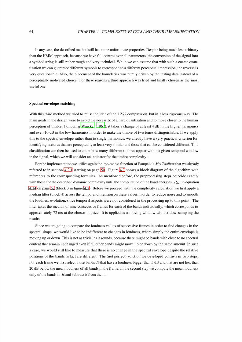
7/29/2019 Streich, S. (2007). Music Complexity. a Multi-faceted Description of Audio Content. Universitat Pompeu Fabra.
http://slidepdf.com/reader/full/streich-s-2007-music-complexity-a-multi-faceted-description-of-audio 81/124
64 CHAPTER 4. COMPLEXITY FACETS AND THEIR IMPLEMENTATION
In any case, the described method still has some unfortunate properties. Despite being much less arbitrary
than the HMM approach, because we have full control over all parameters, the conversion of the signal into
a symbol string is still rather rough and very technical. While we can assume that with such a coarse quan-
tization we can guarantee different symbols to correspond to a different perceptual impression, the reverse is
very questionable. Also, the placement of the boundaries was purely driven by the testing data instead of a
perceptually motivated choice. For these reasons a third approach was tried and finally chosen as the most
useful one.
Spectral envelope matching
With this third method we tried to reuse the idea of the LZ77 compression, but in a less rigorous way. The
main goals in the design were to avoid the necessity of a hard quantization and to move closer to the human
perception of timbre. Following Winckel (1967), it takes a change of at least 4 dB in the higher harmonics
and even 10 dB in the low harmonics in order to make the timbre of two tones distinguishable. If we apply
this to the spectral envelope rather than to single harmonics, we already have a very practical criterion for
identifying textures that are perceptually at least very similar and those that can be considered different. This
classification can then be used to count how many different timbres appear within a given temporal window
in the signal, which we will consider an indicator for the timbre complexity.
For the implementation we utilize again the ma sone function of Pampalk’s MA Toolbox that we already
referred to in section 4.2.1 starting on page 50. Figure 4.7 shows a block diagram of the algorithm with
references to the corresponding formulas. As mentioned before, the preprocessing steps coincide exactly
with those for the described dynamic complexity until the computation of the band energies P dB in equation
4.14 on page 52 (block 3 in figure 4.7). Before we proceed with the complexity calculation we first apply a
median filter (block 4) across the temporal dimension on these values in order to reduce noise and to smooth
the loudness evolution, since temporal aspects were not considered in the processing up to this point. The
filter takes the median of nine consecutive frames for each of the bands individually, which corresponds to
approximately 72 ms at the chosen hopsize. It is applied as a moving window without downsampling the
results.
Since we are going to compare the loudness values of successive frames in order to find changes in the
spectral shape, we would like to be indifferent to changes in loudness, where simply the entire envelope is
moving up or down. This is not as trivial as it sounds, because there might be bands with close to no spectralcontent that remain unchanged even if all other bands might move up or down by the same amount. In such
a case, we would still like to measure that there is no change in the spectral envelope despite the relative
positions of the bands in fact are different. The (not perfect) solution we developed consists in two steps.
For each frame we first select those bands R that have a loudness bigger than 5 dB and that are not less than
20 dB below the mean loudness of all bands in the frame. In the second step we compute the mean loudness
only of the bands in R and subtract it from them.

7/29/2019 Streich, S. (2007). Music Complexity. a Multi-faceted Description of Audio Content. Universitat Pompeu Fabra.
http://slidepdf.com/reader/full/streich-s-2007-music-complexity-a-multi-faceted-description-of-audio 82/124
4.3. TIMBRAL COMPLEXITY 65
Audio signal 1. frame-wise powerspectrum (eq. 4.6 - 4.8)
2. outer ear frequencyweighting (eq. 4.9 - 4.10)
3. spectral spreading applied
on bark band energies
(eq. 4.11 - 4.13)
4. Median filter and loudness
normalization
5. band-wise comparison with
preceding frames (eq. 4.28)
6. detection of segments with
predominant voice
7. percentage of frames with
no similar predecessor (for
non-voice frames)
Timbral
complexity
Figure 4.7: Block diagram of timbral complexity computation based on spectral envelope matching.
The obtained loudness values P [i]sub of each frame i are then compared to those of a group of preceding
frames (block 5):
S [i] =
i−500k=i−10
css
P [i]sub, P
[k]sub
, (4.28)
where the function css(a, b) returns 1 if the absolute difference of all corresponding values in the vectors a
and b is smaller than 6, and zero otherwise. We chose the value of 6 dB, because with 4 dB the tolerance
appeared too small and only very few frames were found as being similar in timbre. The respective time
window starts 80 ms before the current frame and reaches back until 4 s, resembling again roughly human
short-term memory.
In figure 4.8 we see three examples of the resulting function S [i]. The plots emphasize more on the
amount of similar frames that have been found with the method, which is only one way to look at the timbre
complexity or the timbre simplicity rather. We found it more robust however, to consider the percentage of
frames that have no similar frame in the given time window as the indicator of timbre complexity (block 7).
For the bagpipe music in plot a) there are most of the time a considerable amount of similar frames in the past.
It is rare that no similar frame at all can be found and the function reaches zero (8.5% of the frames). Theexcerpt of the classical symphony played by a full orchestra shown in plot b) is usually on slightly lower level
than the bagpipe music indicating a higher variability in the timbre. It also touches the zero mark a bit more
often, which means there are more often timbres appearing that have no correspondence in the recent history
of the signal (11.3%). All this reflects very well the perceived impression when listening to the excerpts. Plot
c) with the rap excerpt marks an extreme case. Despite the perceived timbre does not change that much, the
spectral envelope is completely dominated by the fast changing formants of the speaking voice. Only at the
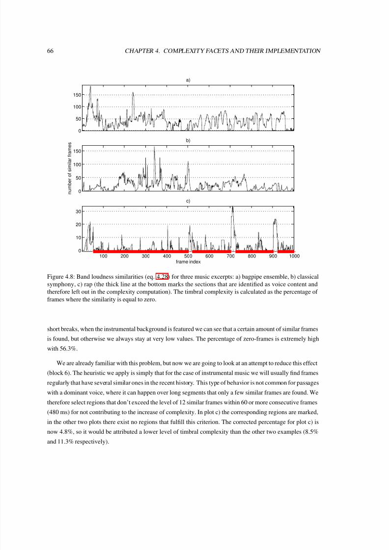
7/29/2019 Streich, S. (2007). Music Complexity. a Multi-faceted Description of Audio Content. Universitat Pompeu Fabra.
http://slidepdf.com/reader/full/streich-s-2007-music-complexity-a-multi-faceted-description-of-audio 83/124
66 CHAPTER 4. COMPLEXITY FACETS AND THEIR IMPLEMENTATION
0
50
100
150
a)
0
50
100
150
n
u m b e r o f s i m i l a r f r a m e s
b)
100 200 300 400 500 600 700 800 900 10000
10
20
30
frame index
c)
Figure 4.8: Band loudness similarities (eq. 4.28) for three music excerpts: a) bagpipe ensemble, b) classical
symphony, c) rap (the thick line at the bottom marks the sections that are identified as voice content and
therefore left out in the complexity computation). The timbral complexity is calculated as the percentage of
frames where the similarity is equal to zero.
short breaks, when the instrumental background is featured we can see that a certain amount of similar frames
is found, but otherwise we always stay at very low values. The percentage of zero-frames is extremely high
with 56.3%.
We are already familiar with this problem, but now we are going to look at an attempt to reduce this effect
(block 6). The heuristic we apply is simply that for the case of instrumental music we will usually find frames
regularly that have several similar ones in the recent history. This type of behavior is not common for passageswith a dominant voice, where it can happen over long segments that only a few similar frames are found. We
therefore select regions that don’t exceed the level of 12 similar frames within 60 or more consecutive frames
(480 ms) for not contributing to the increase of complexity. In plot c) the corresponding regions are marked,
in the other two plots there exist no regions that fulfill this criterion. The corrected percentage for plot c) is
now 4.8%, so it would be attributed a lower level of timbral complexity than the other two examples (8.5%
and 11.3% respectively).

7/29/2019 Streich, S. (2007). Music Complexity. a Multi-faceted Description of Audio Content. Universitat Pompeu Fabra.
http://slidepdf.com/reader/full/streich-s-2007-music-complexity-a-multi-faceted-description-of-audio 84/124
4.4. TONAL COMPLEXITY 67
4.4 Tonal Complexity
In section 3.2.1 of the previous chapter we saw that very well studied models are available for the assessment
of melodic complexity based on a symbolic representation. When it comes to musical audio however, this
facet of complexity can be considered the most difficult one. This is due to melody being a very abstract de-
scription which is hard to access from the audio signal. As pointed out, there is no extraction algorithm avail-
able yet, that can reliably transcribe the melody of just any musical audio file. The situation with harmonic
complexity gives a similar picture. While it is still possible to handle the complexity of chord progressions
that are given as symbolic sequences, we are facing big problems if we need to start from the audio signal
level. It was therefore decided in this dissertation to give up the separation between a melodic and a harmonic
component of music complexity. Instead we only want to consider a tonal complexity facet that accounts for
both, but on a very low level of abstraction. The idea is to work with a signal representation that contains
the important characteristics of the tonal content while not aiming for an exact transcription of single notes
and chords. Based on this representation we can then apply again principles of complexity estimation that we
discussed before.
4.4.1 Implementations of Tonal Complexity
We chose to work with the harmonic pitch class profile feature (HPCP) that has been extensively studied
and developed by Gomez (2004). Its abilities in characterizing tonal content have been demonstrated in
terms of key detection, version identification [Gomez (2006)], and musical structure analysis [Ong (2006)].
Also several approaches towards chord segmentation and recognition rely on this or very similar features
[e. g. Fujishima (1999), Sheh and Ellis (2003)]. We will recapitulate the computation of this feature only
briefly here and refer to the given references for a detailed description. The HPCP is computed frame-wise
in the frequency domain, so the audio signal needs to be segmented into frames, weighted with a window
function, and transformed via Fourier transform. Our settings for frame and hop size are 93 ms and 46 ms
respectively. In order to reduce the influence of non-tonal components in the spectrum, only the local maxima
within a certain frequency range (in our case from 40 Hz to 5 kHz) are considered for further processing.
Some spectral envelope adjustments are done on these peaks to compensate for effects of timbre and for the
presence of overtones. The final feature is then obtained by accumulating the spectral content mapped down
into the range of one octave. We are using a resolution of 36 bins for the pitch classes, which means that each
semitone step covers 3 bins in our HPCP feature vector.
The HPCP vectors can now be used in different ways to arrive at higher semantic levels related with
music tonality. Gomez (2006) correlates them (averaged along time) with ring-shifted key profiles for minor
and for major keys. If the maximum correlation among these alternatives exceeds a certain threshold, she
takes it as an indicator for the key and mode of the musical piece. Depending on the time frame one uses
for the averaging it is possible to move from the global key of the entire piece towards more and more
detailed representations, where modulations to other keys or even individual chords become recognizable.

7/29/2019 Streich, S. (2007). Music Complexity. a Multi-faceted Description of Audio Content. Universitat Pompeu Fabra.
http://slidepdf.com/reader/full/streich-s-2007-music-complexity-a-multi-faceted-description-of-audio 85/124
68 CHAPTER 4. COMPLEXITY FACETS AND THEIR IMPLEMENTATION
Gomez and Herrera (2004) proposed to use the maximum correlation value of the entire file as a descriptor
they named tonal strength. This idea is very straightforward, since it is based on the threshold of this value she
is able to distinguish atonal from tonal music in her key detection processing. A piece where the distribution
of energy on the pitch classes matches very well with the general profile would thus be considered as having
a high tonal strength. The concept behind this is very close to what we are looking for in terms of tonal
complexity, especially considering that the general profiles are inspired from probe tone experiments with
human listeners [Krumhansl (1990)]. So we could think of the profiles as a kind of prototype for the “common
sense” of musical key properties that can be (or not) matched by an actual composition. We therefore included
the tonal strength descriptor into our set of complexity descriptors.
But the descriptor does not cover every aspect of tonal complexity that could be relevant to a human
listener. By its nature, the “tonal strength” is very focused on a statistical picture of tonality. This means
however, that the temporal aspects are not accounted for at all. The rate of changes or the perceptual distance
between consecutive chords for example are not reflected in the tonal strength while they should contribute to
the overall tonal complexity description. We therefore chose an additional approach particularly targeting the
temporal aspects of tonality evolution. If we consider the quantification of tonal change from a musicological
point of view this is not at all trivial. Not only would we need to identify the boundaries where a tonal
unit6 starts and ends, we would also need to label these units. Based on these labels we could then apply a
distance measure like for example the one proposed by Chew (2003) to assess the tonal distances covered in
the course of the piece. Since both, the segmentation and the labeling, are very error-prone with currently
available algorithms, we tried to look for an alternative on a lower abstraction level. As a first idea we
considered to map the sequence of HPCP vectors directly into the three-dimensional space of Chew’s spiral
array. This representation is particularly attractive, since Chew claims that spatial distances in her modelcoincide with musicological ones. By assigning each pitch class on the spiral a virtual mass based on the
accumulated energy of the corresponding HPCP element, we were able to compute a virtual center of gravity
for each vector. From the distance of consecutive centers we hoped then to get an estimation of the tonal
distance. It turned out, however, that the contrast between relevant and irrelevant pitch classes in the HPCP
vector often was not high enough and that even for a perceptually stable tonal unit the proportion of the pitch
classes could vary considerably. As a result, the virtual centers of gravity were located most of the time rather
close to the center of the spiral and their movement did not reflect the tonal properties as expected.
For this reason we modified the approach putting less emphasis on the musicological distance in an
absolute space and more on the amount of relevant fluctuation in the HPCP feature relative to the recent
history of the tonal evolution in the piece. As a preprocessing step we first excluded silent and transient(i. e. not tonal) frames from the computation. This was done by applying a threshold for the minimum frame
energy and the minimum contrast within each HPCP vector. For a tonal frame we can expect a concentration
of energy in only a few elements of the vector, whereas in transient frames the energy is more equally
distributed yielding a lower contrast. We then compute two moving averages T [i]1 (m) and T
[i]2 (m) with
6This can be either in the concrete sense of a specific group of pitches sounding simultaneously, or more abstract in the sense of
harmonic functions of chords.

7/29/2019 Streich, S. (2007). Music Complexity. a Multi-faceted Description of Audio Content. Universitat Pompeu Fabra.
http://slidepdf.com/reader/full/streich-s-2007-music-complexity-a-multi-faceted-description-of-audio 86/124
4.4. TONAL COMPLEXITY 69
different window sizes individually on each of the HPCP vector dimensions. T [i]1 (m) is supposed to reflect
the local tonal context and covers 250 frames (approx. 11.5 s), T [i]2 (m) corresponds to the instantaneous
tonal content and covers 25 frames (approx. 1.15 s). Each vector of the two series is then normalized to a
maximum of one.
Now we compute two different distance measures between the corresponding elements of T 1 and T 2. That
means for each frame i we compare the instantaneous tonal content T [i]2 averaged over the past 25 frames to
the bigger tonal context T [i]1 established during the past 250 frames. One criterion for the comparison is the
overall similarity of the shape. We measure this with the Pearson correlation coefficient:
r[i] =
M m=1(T
[i]1 (m) − T
[i]1 )(T
[i]2 (m) − T
[i]2 )
(M − 1) · T [i]1 T
[i]2
, (4.29)
where x and x denote the mean and the standard deviation of a vector x, respectively. M refers to thedimensionality of the pitch class vectors, which is 36 in our case. Negative values for r[i] are set to zero,
since we are only interested in the degree to which the two vectors are similar in shape. Negative correlations
are therefore not relevant for us. Since we want a distance rather than a similarity measure, we then invert the
correlation through D[i]1 = 1 − r[i].
We found in empirical tests that the Pearson correlation alone did not yield the desired results under
certain circumstances. If for example a chord is sounding for some time and then one of its pitches is
disappearing or an additional one joins in while the rest remains, then the correlation measure does not show
a clear response. Overall it appears to react mainly to major shifts and changes in the tonal configuration
and to be rather insensitive to changes of only single pitches. An example of this can be seen in figure 4.9
shortly before frame number 400. While there are changes taking place in the lowest HPCP bins and around
bin number 19, the correlation measure does not show any reaction.
For this reason we included a second distance measure that shows a higher sensitivity to these types of
fluctuations. For this purpose we first quantize the two vector sequences T 1 and T 2 to three levels. Values
bigger than 0.5 are considered relevant tonal components and are assigned a value of 2. Values below 0.001
are most certainly irrelevant components and therefore assigned a value of zero. The rest of the values cannot
be assigned to either group with high certainty or belong into transition periods and therefore are assigned a
value of 1. We then compute the city block distances between the corresponding vectors of either sequence
D[i]
2
=36
m=1
T [i]
q1(m) − T
[i]
q2(m) . (4.30)
The city block metric is preferred at this point over the euclidian or other distance measures. This is because
it corresponds more directly to the number of elements that changed in the vector, which is in fact what we
want to be reflected better in our complexity measure. We can see in figure 4.9 that this measure responds
with a clear peak to the changes that take place shortly before frame number 400. However, when there are
many active pitches the indications of this measure are less reliable. For example the major shift around

7/29/2019 Streich, S. (2007). Music Complexity. a Multi-faceted Description of Audio Content. Universitat Pompeu Fabra.
http://slidepdf.com/reader/full/streich-s-2007-music-complexity-a-multi-faceted-description-of-audio 87/124
70 CHAPTER 4. COMPLEXITY FACETS AND THEIR IMPLEMENTATION
0
0.2
0.4
0.6
0.8
a)
0
10
20
b)
d i s t a n c e
0
5
10
c)
frame index
H P C P b i n
100 200 300 400 500 600
10
20
30
Figure 4.9: Distance measures for tonal complexity computation: a) inverted correlation D[i]1 , b) city block
distance D[i]2 , c) linear combination, d) corresponding HPCP data (before moving average).

7/29/2019 Streich, S. (2007). Music Complexity. a Multi-faceted Description of Audio Content. Universitat Pompeu Fabra.
http://slidepdf.com/reader/full/streich-s-2007-music-complexity-a-multi-faceted-description-of-audio 88/124
4.5. RHYTHMIC COMPLEXITY 71
frame 600 is detected much clearer by the correlation measure. As a final indicator for the tonal complexity,
we take therefore the average of the combined distance measures over all N frames7 of the piece:
C tonal =1
N
N i=1
D[i]1 · D
[i]2 . (4.31)
4.5 Rhythmic Complexity
With the PS-measure, that we reviewed in section 3.2.2, we have already seen a model for rhythmic complex-
ity that even has been assessed to a certain degree in tests with human subjects. But as we observed already,
the applicability of the model in our context is questionable, since it operates on an abstraction level which
is not easy to achieve when starting from the audio signal. Furthermore, 3.2.2 performed their experiments
with short rhythm patterns in isolation. It is not clear whether the perceived complexity of such a pattern isexactly the same when it is part of a complete musical performance in a larger temporal context.
We therefore will put our focus more on questions like: Is there a clear rhythm in the music? Is it strongly
induced? Is it stable? Does it happen in a usual speed? On a rather na ıve level, we could also formulate: Is it
easy to clap along with the music? Is the music easy to dance to?
These questions lead us to the conclusion that the type of rhythmic complexity we are after has to be
found on a level of lower abstraction and specialization than that of the PS-Measure. The danceability de-
scriptor based on the detrended fluctuation analysis that we already mentioned in section 3.3.3 is therefore an
interesting candidate as it works directly on the time domain signal without making any assumptions about
the metric grid or even note onsets. The error-prone transcription or event detection procedures can thus be
avoided.
4.5.1 Implementation of Danceability
The implementation described here is following the description by Jennings et al. (2004). Where exact spec-
ifications were missing, we integrated reasonable solutions. The experimental findings obtained with this im-
plementation on a large music database were also reported at the 118th AES Convention [Streich and Herrera
(2005)].
As a first step the audio signal is segmented into non-overlapping blocks of 10 ms length. For each
block the standard deviation s(n) of the amplitude is computed. The values s(n) resemble a bounded, non-
stationary time series, which can be associated with the averaged physical intensity of the audio signal ineach block (see figure 4.10). In order to obtain the unbounded time series y(m), s(n) is integrated:
y(m) =mn=1
s(n) (4.32)
7As we said, only the presumably tonal frames are considered here.

7/29/2019 Streich, S. (2007). Music Complexity. a Multi-faceted Description of Audio Content. Universitat Pompeu Fabra.
http://slidepdf.com/reader/full/streich-s-2007-music-complexity-a-multi-faceted-description-of-audio 89/124
72 CHAPTER 4. COMPLEXITY FACETS AND THEIR IMPLEMENTATION
0
0.5
1classic
0
0.5
1
I n t e n s i t y ( n o r m a l i z e d )
techno
0 5 10 150
0.5
1
time in s
pop
Figure 4.10: Excerpts from the time series s(n) for three example pieces from different musical genres.
This integration step is crucial in the process of Detrended Fluctuation Analysis (DFA) computation,
because for bounded time series the DFA exponent (our final feature) would always be 0 when time scales of
greater size are considered. This effect is explained in more detail in Peng (2005).
The series y(m) can be thought of as a random walk in one dimension. y(m) is now again segmented
into blocks of τ elements length. This time, we advance only by one sample from one block to the next in the
manner of a sliding window. There are two reasons for this extreme overlap. First, we obtain more blocks
from the signal, which is of interest, since we will obtain better statistics from a larger number of blocks.
Secondly, we avoid possible synchronization with the rhythmical structure of the audio signal, which would
lead to arbitrary results depending on the offset we happen to have. However, performing the computation in
this manner the number of operations is increased enormously8.
From each block we now remove the linear trend yk and compute D(k, τ ), the mean of the squared
residual:
D(k, τ ) =1
τ
τ −1m=0
(y(k + m) − yk(m))2
(4.33)
We then obtain the detrended fluctuation F (τ ) of the time series by computing the square root of the
8In order to reduce the computational load it was found empirically that gently increasing the hopsize with growing window size
does not affect the quality of the results too much (e. g. hopsize = windowsize/50).

7/29/2019 Streich, S. (2007). Music Complexity. a Multi-faceted Description of Audio Content. Universitat Pompeu Fabra.
http://slidepdf.com/reader/full/streich-s-2007-music-complexity-a-multi-faceted-description-of-audio 90/124
4.5. RHYTHMIC COMPLEXITY 73
0.3 0.5 0.7 1.2 2 3 5 8−1.5
−1
−0.5
0
0.5
time scale in s
l o g 1 0
( F )
classictechno
pop
Figure 4.11: Double logarithmic plots of mean residual over time scales.
mean of D(k, τ ) for all K blocks:
F (τ ) = 1
K
K k=1 D(k, τ ) (4.34)
As indicated, the fluctuation F is a function of τ (i. e. of the time scale in focus). The goal of DFA is
to reveal correlation properties on different time scales. We therefore repeat the process above for different
values of τ that are within the range of our interest. Jennings et al. (2004) use a range from 310 ms (τ = 31)
to 10 s not specifying the step size in their paper. Relating these time scales to the musical signal they cover
the beat level to the bar level and reach further up to the level of longer rhythmical patterns.
The DFA exponent α is defined as the slope of the double logarithmic graph of F over τ (eq. 4.35)
as shown in figure 4.11 for the three example tracks. It therefore makes sense to increase τ by a constant
multiplication factor rather than a fixed step size. Apart from giving equally-spaced supporting points on
the logarithmic axis it also reduces the computational operations without affecting the accuracy greatly. We
chose a factor of 1.1 giving us 36 different values for τ covering time scales from 310 ms to 8.8 s.
For small values of τ an adjustment is needed in the denominator when computing α (see Buldyrev et al.
(1995)) giving us the following formula for the DFA exponent:
α(i) =log10 (F (τ i+1)/F (τ i))
log10 ((τ i+1 + 3)/(τ i + 3))(4.35)
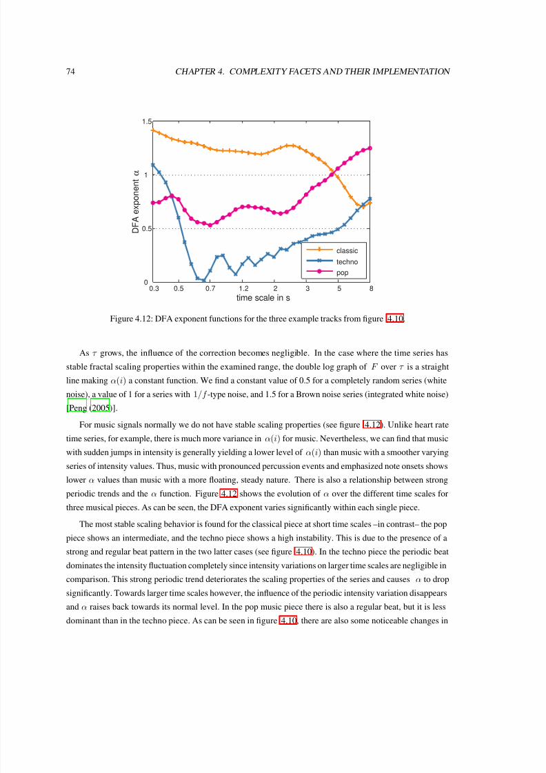
7/29/2019 Streich, S. (2007). Music Complexity. a Multi-faceted Description of Audio Content. Universitat Pompeu Fabra.
http://slidepdf.com/reader/full/streich-s-2007-music-complexity-a-multi-faceted-description-of-audio 91/124
74 CHAPTER 4. COMPLEXITY FACETS AND THEIR IMPLEMENTATION
0.3 0.5 0.7 1.2 2 3 5 80
0.5
1
1.5
time scale in s
D F A e x p o n e n t α
classic
techno
pop
Figure 4.12: DFA exponent functions for the three example tracks from figure 4.10.
As τ grows, the influence of the correction becomes negligible. In the case where the time series has
stable fractal scaling properties within the examined range, the double log graph of F over τ is a straight
line making α(i) a constant function. We find a constant value of 0.5 for a completely random series (white
noise), a value of 1 for a series with 1/f -type noise, and 1.5 for a Brown noise series (integrated white noise)
[Peng (2005)].
For music signals normally we do not have stable scaling properties (see figure 4.12). Unlike heart rate
time series, for example, there is much more variance in α(i) for music. Nevertheless, we can find that music
with sudden jumps in intensity is generally yielding a lower level of α(i) than music with a smoother varying
series of intensity values. Thus, music with pronounced percussion events and emphasized note onsets shows
lower α values than music with a more floating, steady nature. There is also a relationship between strong
periodic trends and the α function. Figure 4.12 shows the evolution of α over the different time scales for
three musical pieces. As can be seen, the DFA exponent varies significantly within each single piece.
The most stable scaling behavior is found for the classical piece at short time scales –in contrast– the pop
piece shows an intermediate, and the techno piece shows a high instability. This is due to the presence of astrong and regular beat pattern in the two latter cases (see figure 4.10). In the techno piece the periodic beat
dominates the intensity fluctuation completely since intensity variations on larger time scales are negligible in
comparison. This strong periodic trend deteriorates the scaling properties of the series and causes α to drop
significantly. Towards larger time scales however, the influence of the periodic intensity variation disappears
and α raises back towards its normal level. In the pop music piece there is also a regular beat, but it is less
dominant than in the techno piece. As can be seen in figure 4.10, there are also some noticeable changes in

7/29/2019 Streich, S. (2007). Music Complexity. a Multi-faceted Description of Audio Content. Universitat Pompeu Fabra.
http://slidepdf.com/reader/full/streich-s-2007-music-complexity-a-multi-faceted-description-of-audio 92/124
4.5. RHYTHMIC COMPLEXITY 75
intensity on a larger time scale. Still, α is clearly decreased by the periodic trend. Towards larger time scales,
we can observe the same effect as in the techno piece. For the classical piece no dominant, regular beat
pattern can be identified in the time series. Thus, the scaling properties are not affected in the corresponding
range. But in contrast to the other two examples the series reveals a larger scale pattern in some parts, which
can also be seen in figure 4.10. This causes α to drop in the upper range.
In order to arrive at an indicator for the danceability and thus a certain aspect of the rhythmic complexity
the α values have to be further reduced. While different ways are possible, in the first implementation simply
the average α level was computed for each track. A high value refers to a high complexity (not danceable),
a low value refers to a low complexity (highly danceable). In a slightly more sophisticated approach we also
tried to separate the component related to the beat from the one referring to the larger time scales. As can
be clearly observed in figure 4.12 a strong and steady beat causes strong oscillations in the scaling curve.
The stronger the dominance of the induced beat in the music, the lower does the curve of alpha values reach.
Therefore we use the height of the lowest local minimum in the scaling curve for time scales below 1.5 s as an
indicator for the beat strength. As the minima appear roughly at the time scale that corresponds to 1.5 times
the inter-beat interval, the limit of 1.5 s is a lower bound for the tempo coinciding with approximately 60
BPM. This does not necessarily resemble the real perceived tempo, as the strong downbeats might occur only
on every second or third counted beat. We applied a ceiling of 1 for these minima, because values beyond this
limit didn’t seem to reflect anything related with the beat strength anymore. For the part of the curve beyond
the 1.5 s boundary it was not possible to identify any straightforward processing that was more useful than the
simple average. While the beat strength alone can already be considered an alternative rhythmic complexity
descriptor, we also used the linear combination of the beat strength and the average α above 1.5 s.

7/29/2019 Streich, S. (2007). Music Complexity. a Multi-faceted Description of Audio Content. Universitat Pompeu Fabra.
http://slidepdf.com/reader/full/streich-s-2007-music-complexity-a-multi-faceted-description-of-audio 93/124
76 CHAPTER 4. COMPLEXITY FACETS AND THEIR IMPLEMENTATION

7/29/2019 Streich, S. (2007). Music Complexity. a Multi-faceted Description of Audio Content. Universitat Pompeu Fabra.
http://slidepdf.com/reader/full/streich-s-2007-music-complexity-a-multi-faceted-description-of-audio 94/124
Chapter 5
Evaluation
The evaluation of the achievements, which means the critical assessment and determination of worth and
validity, is of fundamental importance in scientific activity. While such a statement is pretty much a com-
monplace it is in fact not always easy in practice to settle this claim in an uncompromising manner. Especially
when dealing with music, which comes in countless styles, forms, and fashions, it is often hard to provide
a test or an experimental setup of far-ranging, solid validity. Furthermore a researcher with a background in
engineering (like the author) might suddenly see himself confronted with the need to borrow methods from
other domains intersecting the MIR field, in order to account for the human factor that enters the equation
when semantic concepts are to be explored.
Only relatively recently have there been efforts in the domain of music information retrieval research to
establish standard-like data sets and metrics for evaluation [e. g. Goto et al. (2002) or Cano et al. (2006)1].
Of course these joint efforts concentrate on “hot topics” or problems that are dealt with by relatively many
researchers from different institutions. This is not the case for music complexity estimation. During this
dissertation different means of evaluation were applied to the developed algorithms. In the following sections
we will first describe these methods before the actual results are reported.
5.1 Methods of Evaluation
The obvious method to validate the developed algorithms of course is an assessment of the agreement between
human complexity perception and the algorithmic predictions. While this is the most direct evaluation it also
involves certain inconveniences. The biggest challenge is the fact that a reasonably big database with music
tracks and the corresponding human complexity ratings is needed. The term “big” is relevant in three different
ways here: First, we need to include music tracks from a variety of styles, since we are after complexity
beyond genre limits. A selection of tracks that is truly representative of the universe of music available in
digital format is hard to establish, but to select multiple examples from many different styles is the least one
1See also http://ismir2004.ismir.net/ISMIR Contest.html and http://www.music-ir.org/mirex2006/
77

7/29/2019 Streich, S. (2007). Music Complexity. a Multi-faceted Description of Audio Content. Universitat Pompeu Fabra.
http://slidepdf.com/reader/full/streich-s-2007-music-complexity-a-multi-faceted-description-of-audio 95/124
78 CHAPTER 5. EVALUATION
can do to approximate generality. Secondly, we would like to have complexity ratings for each item by many
different subjects. This is because we are interested in a “common sense” of complexity. By combining the
ratings of a group of subjects we can reduce the influence of outlier responses due to individual preference
or peculiarity. Thirdly, it would be ideal to assess complexity ratings separately for each of the facets we
are considering. In this way, it would be possible to evaluate each of the algorithms in isolation and avoid
mediating effects among the facets. However, human ratings of good quality are not so easy to obtain. Due
to practical necessities and limitations we need to accept compromises regarding these three aspects. We will
talk in detail about this way of evaluation in section 5.2. A very similar approach would be to pay a group of
people for manually labelling a set of songs according to the different facets of complexity. This is dangerous
since the quality of the annotations is difficult to check and somebody assigning random labels could spoil
the entire data set. One could overcome this effect by using many people in order to identify outliers, but this
makes the approach very costly.
Although the mentioned assessment is the most straightforward one, it could be interesting as well, to
focus more on the usefulness of complexity descriptors in the MIR context. After all, we are not after
music complexity as a stand-alone quality for its own sake. The application of this research is in facilitating
the management of music collections in terms of organization, visualization, and browsing for example.
From this point of view there are of course other ways of evaluation that come to mind. It is possible for
example to use selected complexity descriptors together with machine learning methods in order to evaluate
their discriminative power in genre, artist, or other classification based on semantic labels. Although the
descriptors might not be used in exactly the same way in a final application, at least an experimental proof
of relevance can be established if the classification reaches significantly beyond chance level. This approach
is of course less powerful in terms of scientific argument, but it bears the advantage that there is no needfor costly annotations or user experiments, since many semantic labels are easily available in existing test
collections. This strategy of evaluation will be reported in section 5.3. Another option along the same line
is the testing of user preferences in an actual music selection task. So rather than comparing the algorithmic
predictions with human ratings of complexity, one can directly use the computed descriptors for organizing
a collection and then test whether this facilitates measurably the users’ interaction with the music compared
to alternative ways of organization. Section 5.4 will describe briefly such an experiment and the obtained
results.
Probably the weakest, but also the easiest method of evaluation is through artificial test cases. We can
select, compose, generate, or modify music material in order to match a specific level of complexity according
to our own definitions. This is basically reversing the process of annotating a ground truth to a given set of
data. Instead, we start by deciding on the label and only afterwards look for the right content. We mentioned
this type of evaluation already in section 4.3 of the previous chapter. There we selected several music samples
according to specified levels of timbral complexity and used them as reference points in our experiments.
However, this approach cannot avoid to be subjected to criticism. The reasoning about the validity of the
algorithms can become circular, if we orient ourselves too close to the algorithm itself during the creation or

7/29/2019 Streich, S. (2007). Music Complexity. a Multi-faceted Description of Audio Content. Universitat Pompeu Fabra.
http://slidepdf.com/reader/full/streich-s-2007-music-complexity-a-multi-faceted-description-of-audio 96/124
5.2. EVALUATION WITH HUMAN RATINGS 79
selection of the test data. In such a case, we will only be able to verify that the implementation is correct.
Whether the algorithm really has anything to say about music complexity however could not be proved
this way. But even if the test material is chosen with more care, as in the case of our timbral complexity
experiments, there is always the question of objectivity overshadowing the results. In fact there would be
the need to validate the test material with a separate evaluation in order to prove that it is not biased. This
of course closes the circle to the first method of evaluation that was mentioned above with all its problems.
Since we are dealing with music, the easiness of the generation is also very relative. It can be quite difficult
to control all the mentioned facets of complexity.
5.2 Evaluation with Human Ratings
As mentioned above, ideally we would like to have the complexity ratings for hundreds of pieces of music
from hundreds of people broken down into all of the facets that we have been considering in the previous
chapter. We would appreciate a wide range of musical styles being represented and having people with very
different musical preference and experience, as long as they belong to our targeted group (i. e. they have a
western cultural musical background). However, we are not living in an ideal world and therefore we have to
accept compromises. As it was not feasible to obtain ground truth complexity ratings locally from “annotation
mercenaries”, the alternative of a web-based survey was realized instead.
5.2.1 Survey Design, Material, and Subjects
The survey was adapted from the version used in Sandvold and Herrera (2005) and consisted of two parts.
First, subjects had to fill in some data regarding their age, sex, musical experience, and music listening habits.
The second part consisted of the actual rating phase where 30 s excerpts of music recordings were presented
in a randomized order. Subjects had to indicate their familiarity with the music, their complexity judgement
and their liking of it. They were allowed repeated playback and correction of their ratings until they clicked
on the “Continue” button. Figure 5.1 shows a screen-shot of the second part of the survey.
The survey was provided in three languages (English, Spanish and German) in order to encourage as many
subjects as possible for participation. This way we also intended to avoid misunderstandings due to language
problems. The order of question 2 and 3 (complexity and liking) was switched for every other subject in
order to check for an influence in the ratings. As the explicit rating of music complexity is not a common
task, we provided some guidance to the participants on how they might come to a decision. By clicking on
“help” next to the question about complexity the subjects could open a window with the following text:
Judging Music Complexity
The complexity of music is not as intuitive as liking or familiarity.
We therefore want to give you some help on how to find an answer.
When listening to the music try to consider the following questions:
• How much is going on in the music?

7/29/2019 Streich, S. (2007). Music Complexity. a Multi-faceted Description of Audio Content. Universitat Pompeu Fabra.
http://slidepdf.com/reader/full/streich-s-2007-music-complexity-a-multi-faceted-description-of-audio 97/124
80 CHAPTER 5. EVALUATION
Figure 5.1: Screenshot from the second part of the websurvey.

7/29/2019 Streich, S. (2007). Music Complexity. a Multi-faceted Description of Audio Content. Universitat Pompeu Fabra.
http://slidepdf.com/reader/full/streich-s-2007-music-complexity-a-multi-faceted-description-of-audio 98/124
5.2. EVALUATION WITH HUMAN RATINGS 81
• Is it completely predictable or very surprising?
• Can you easily follow the music?
• Or is it demanding a high effort?
With this in mind you will hopefully be able to select the appropriate
option without difficulty. The music examples presented here were
chosen to cover the entire range of complexity levels. Don’t feel
shy to use the extreme ratings if you consider it appropriate.
The total number of music excerpts was 82, out of which a maximum of 30 were randomly selected for
each participant. The disadvantage of this procedure is that we have a different subset of songs rated by
each subject, which limits in a certain way the possibilities for analyses. We chose this design, because it
allows for a larger number of songs to be rated while keeping the time subjects had to spent answering the
survey in reasonable limits. For the selection of audio material we took care of having very diverse musical
styles in the data set including a few famous songs that participants are very likely to be familiar with. The
majority of songs however was taken from less famous artists, while still being at a professional level of
musical and technical quality. The styles included some branches of classical music, diverse productions
from the Pop and Rock genres, Techno and Electronic Dance Music, Jazz and World Music, and several
modern compositions of electro-acoustic music. In selecting the music for this experiment we put a higher
emphasis on covering a wide range of complexity levels in the different facets rather than on a proportional or
representative distribution of the styles. The excerpts were extracted in an automatic fashion, by cutting out a
30 s segment from the recording starting at 20 s after the beginning. We used RMS power normalization on
the excerpts in order to achieve a more or less similar loudness level for all stimuli. The excerpts were checked
afterwards and those considered not appropriate for the survey were replaced by a manually selected segment
from the corresponding track. For reasons of bandwidth economy the tracks were made available only in
the compressed ISO-MPEG-1 layer 3 format commonly known as MP3 [ Brandenburg and Stoll (1994)]. We
used an implementation derived from the LAME2 project for this purpose applying a fixed bit rate of 128 kbps
in stereo mode. At this bit rate setting, the audio signal is only preserved up to roughly 17 kHz, which results
in a very good but not totally transparent quality. As many of the tracks had been compressed before and
were not available to us in their original release format, there was a danger of audible transcoding artifacts.
It was made sure through inspection of the files that they were free of such disturbing effects.
We invited friends, students, and colleagues by email to participate. An announcement in the Freesoundforum3 proved to be the most effective way to win participants. Although participation was completely volun-
tary and there was no benefit for the subjects other than satisfying their curiosity and potentially discovering
new music, there was a relatively big interest in the topic. 207 subjects started answering and 124 of them fin-
ished the entire experiment consisting in the rating of 30 music excerpts. Table 5.1 shows some statistics for
2http://lame.sourceforge.net/ 3http://freesound.iua.upf.edu/index.php

7/29/2019 Streich, S. (2007). Music Complexity. a Multi-faceted Description of Audio Content. Universitat Pompeu Fabra.
http://slidepdf.com/reader/full/streich-s-2007-music-complexity-a-multi-faceted-description-of-audio 99/124
82 CHAPTER 5. EVALUATION
gender age in years musical knowledge total
male female 15-24 25-35 36-63 none basic advanced professional
Count: 125 17 57 58 27 10 22 70 40 142%: 88.0 12.0 40.1 40.8 19.0 7.0 15.5 49.3 28.2
Table 5.1: Statistics about the subjects who answered the web survey.
the subjects whose ratings have been used in the evaluation4. One disadvantage of a web survey revealed here
is that the composition of subjects is unbalanced. We have a strong prevalence of male and young subjects.
Probably the most disadvantageous condition for our needs is the low number of subjects with low musical
training, since we are preferably interested in the complexity perception of non-expert listeners. But as the
presented excerpts have been taken from a wide variety of styles we hope that even for the highly trained
subjects the effects of expertise are not predominant.
5.2.2 The Obtained Data
As a first step after the survey page was closed we did some statistical analysis on the subjects’ data and the
ratings. As mentioned in table 5.1 we used the ratings of a total of 142 subjects in our analyses. With a total
of 3545 ratings we had on average about 43 ratings per excerpt to work with. Comparing the averaged ratings
of complexity and liking per song for the two groups with and without switched question order there was no
significant difference. Neither had the order of presentation of the excerpts any significant effect on these
ratings.
When we performed a one-way ANOVA on either type of ratings with the stimulus (the excerpt ID) being
the independent variable we obtained a significant F-score in both cases. Precisely we got F = 16.09 for
the complexity ratings and F = 7.57 for the ratings of liking. With 81 degrees of freedom both values
are strongly significant ( p < 0.001) suggesting that the individual excerpts are indeed receiving clearly
distinguishable responses in the statistical sense. With the much higher F-score for the complexity ratings
we further have evidence that the agreement on complexity judgements among the subjects is higher than
for judgements of liking, since the amount of variance explained by selecting the stimulus is bigger. This
goes along well with our idea of a “common sense” of music complexity perception opposed to the different
personal tastes and therefore higher subjectivity reflected in the ratings of liking for the stimuli.
We computed a set of 12 complexity descriptors that were presented in the previous chapter on all 82
music excerpts. A standardization to zero mean and unity variance was performed before proceeding with
the analyses. The descriptor set consisted of:
C dynI the dynamic component of acoustic complexity based on Vickers’ method (eq. 4.5, page 47).
C dynII the dynamic component of acoustic complexity based on Pampalk’s implementation (eq. 4.18, page
50).
4All subjects that submitted at least five ratings were considered.
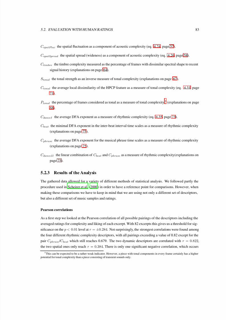
7/29/2019 Streich, S. (2007). Music Complexity. a Multi-faceted Description of Audio Content. Universitat Pompeu Fabra.
http://slidepdf.com/reader/full/streich-s-2007-music-complexity-a-multi-faceted-description-of-audio 100/124
5.2. EVALUATION WITH HUMAN RATINGS 83
C spatFluc the spatial fluctuation as a component of acoustic complexity (eq. 4.24, page 57).
C spatSpread the spatial spread (wideness) as a component of acoustic complexity (eq. 4.26, page 58).
C timbre the timbre complexity measured as the percentage of frames with dissimilar spectral shape to recent
signal history (explanations on page 64).
S tonal the tonal strength as an inverse measure of tonal complexity (explanations on page 67).
C tonal the average local dissimilarity of the HPCP feature as a measure of tonal complexity (eq. 4.31, page
71).
P tonal the percentage of frames considered as tonal as a measure of tonal complexity5 (explanations on page
68).
C danceI the average DFA exponent as a measure of rhythmic complexity (eq. 4.35, page 73).
C beat the minimal DFA exponent in the inter-beat interval time scales as a measure of rhythmic complexity
(explanations on page 75).
C phrase the average DFA exponent for the musical phrase time scales as a measure of rhythmic complexity
(explanations on page 75).
C danceII the linear combination of C beat and C phrase as a measure of rhythmic complexity(explanations on
page 75).
5.2.3 Results of the Analysis
The gathered data allowed for a variety of different methods of statistical analysis. We followed partly the
procedure used in Scheirer et al. (2000) in order to have a reference point for comparisons. However, when
making these comparisons we have to keep in mind that we are using not only a different set of descriptors,
but also a different set of music samples and ratings.
Pearson correlations
As a first step we looked at the Pearson correlation of all possible pairings of the descriptors including the
averaged ratings for complexity and liking of each excerpt. With 82 excerpts this gives us a threshold for sig-nificance on the p < 0.01 level at r = ±0.284. Not surprisingly, the strongest correlations were found among
the four different rhythmic complexity descriptors, with all pairings exceeding a value of 0.82 except for the
pair C phrase / C beat which still reaches 0.679. The two dynamic descriptors are correlated with r = 0.822,
the two spatial ones only reach r = 0.384. There is only one significant negative correlation, which occurs
5This can be expected to be a rather weak indicator. However, a piece with tonal components in every frame certainly has a higher
potential for tonal complexity than a piece consisting of transient sounds only.
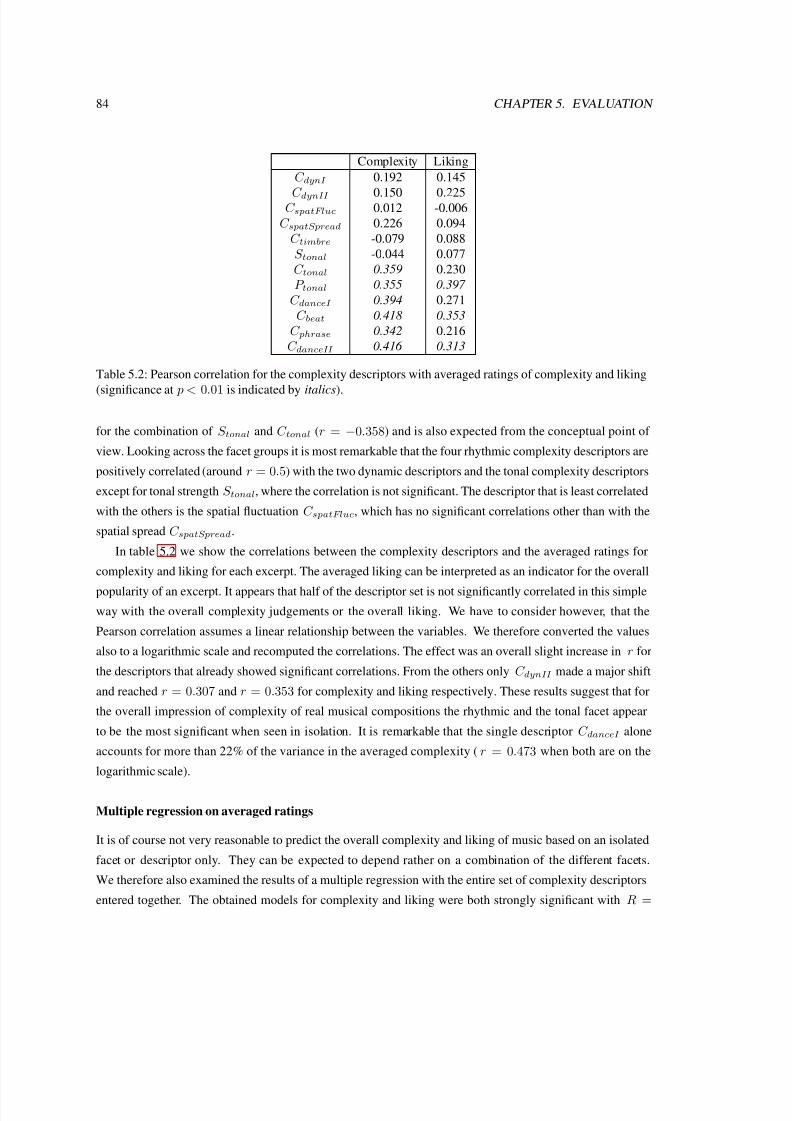
7/29/2019 Streich, S. (2007). Music Complexity. a Multi-faceted Description of Audio Content. Universitat Pompeu Fabra.
http://slidepdf.com/reader/full/streich-s-2007-music-complexity-a-multi-faceted-description-of-audio 101/124
84 CHAPTER 5. EVALUATION
Complexity Liking
C dynI 0.192 0.145
C dynII 0.150 0.225C spatFluc 0.012 -0.006
C spatSpread 0.226 0.094
C timbre -0.079 0.088
S tonal -0.044 0.077
C tonal 0.359 0.230
P tonal 0.355 0.397
C danceI 0.394 0.271
C beat 0.418 0.353
C phrase 0.342 0.216
C danceII 0.416 0.313
Table 5.2: Pearson correlation for the complexity descriptors with averaged ratings of complexity and liking
(significance at p < 0.01 is indicated by italics).
for the combination of S tonal and C tonal (r = −0.358) and is also expected from the conceptual point of
view. Looking across the facet groups it is most remarkable that the four rhythmic complexity descriptors are
positively correlated (around r = 0.5) with the two dynamic descriptors and the tonal complexity descriptors
except for tonal strength S tonal, where the correlation is not significant. The descriptor that is least correlated
with the others is the spatial fluctuation C spatFluc, which has no significant correlations other than with the
spatial spread C spatSpread.
In table 5.2 we show the correlations between the complexity descriptors and the averaged ratings for
complexity and liking for each excerpt. The averaged liking can be interpreted as an indicator for the overall
popularity of an excerpt. It appears that half of the descriptor set is not significantly correlated in this simple
way with the overall complexity judgements or the overall liking. We have to consider however, that the
Pearson correlation assumes a linear relationship between the variables. We therefore converted the values
also to a logarithmic scale and recomputed the correlations. The effect was an overall slight increase in r for
the descriptors that already showed significant correlations. From the others only C dynII made a major shift
and reached r = 0.307 and r = 0.353 for complexity and liking respectively. These results suggest that for
the overall impression of complexity of real musical compositions the rhythmic and the tonal facet appear
to be the most significant when seen in isolation. It is remarkable that the single descriptor C danceI alone
accounts for more than 22% of the variance in the averaged complexity (r = 0.473 when both are on the
logarithmic scale).
Multiple regression on averaged ratings
It is of course not very reasonable to predict the overall complexity and liking of music based on an isolated
facet or descriptor only. They can be expected to depend rather on a combination of the different facets.
We therefore also examined the results of a multiple regression with the entire set of complexity descriptors
entered together. The obtained models for complexity and liking were both strongly significant with R =

7/29/2019 Streich, S. (2007). Music Complexity. a Multi-faceted Description of Audio Content. Universitat Pompeu Fabra.
http://slidepdf.com/reader/full/streich-s-2007-music-complexity-a-multi-faceted-description-of-audio 102/124
5.2. EVALUATION WITH HUMAN RATINGS 85
0.771 and R = 0.736 ( p < 0.001), which means that roughly 60% and 54% of the variance in the data
can be explained by them. For comparison, Scheirer et al. (2000) reached R = 0.536 with their set of 16
psychoacoustic features on 150 musical excerpts (see section 3.3.1 in chapter 3).
While these results are relatively impressive in direct comparison, this also means that around 40% of the
variance in mean complexity per song originate from factors that are not covered by the linear combination
of our descriptor set. One such factor could be the lyrics of the music, which can form an important aspect
in musical judgements [see e. g. Rentfrow and Gosling (2003)]. Another such factor would be the melody, a
facet which is only partly reflected in our tonal complexity descriptors. In general, the sociocultural compo-
nent related with music complexity judgements is not accessed at all by the descriptors in our set (for example
the image of certain musical styles or particular artists). Another very possible source of unexplained vari-
ance is the subjectivity in the ratings, which might have an effect despite averaging over approximately 40
responses per excerpt. The critical point of the chosen survey design in this sense is that the subjects that rated
one particular song are a random sample of the non-homogeneous, non-representative body of participants.
As an example, of two songs that have objectively very similar properties, one might be rated by a sample
dominated by music professionals with an aversion to this musical style, and the other by a sample dominated
by musical laymen who feel indifferent about it.
Logistic regression on individual ratings
We therefore tried also a different analysis by considering individual subject models. Such a model would
try to predict the ratings of only one subject and could therefore adapt better to individual peculiarities in
music complexity judgements. Following Scheirer’s methodology we created two binary variables from the
individual ratings of complexity and liking indicating only whether they were above or below the mean
rating of each subject. We then built a logistic regression models for each individual subject trying to predict
the binarized complexity and liking variables respectively. The models used the complete set of available
complexity descriptors to calculate their predictions. Only the 124 subjects who finished the whole survey
and gave the maximum amount of 30 ratings were considered in this experiment.
With the obtained models 83.0% of the binary complexity ratings and 82.6% of the binary liking ratings
could be predicted correctly (see figure 5.2). Scheirer et al. (2000) obtained 73.6% of correct responses in
their experiment stating that 46.7% of their models gave statistically significant predictions ( p < 0.05). In our
case 55.4% of the user models for complexity predictions and 47.1% of the user models for liking predictions
were significant. Similar to Scheirer we also observed that the use of a single model for all subjects reachesonly slightly above chance level in predicting the ratings of complexity or liking.
The results show on one hand, that by combining the complexity descriptors in different ways we can
adapt to individual peculiarities in the perception of complexity and liking for music and very successfully
predict subjective judgments. On the other hand, for about half of the subjects it was not possible to predict
their ratings significantly better than through guessing. From figure 5.2 we can see the influence of some of
the demographic variables on the performance of the logistic regression models. Most of them are statistically

7/29/2019 Streich, S. (2007). Music Complexity. a Multi-faceted Description of Audio Content. Universitat Pompeu Fabra.
http://slidepdf.com/reader/full/streich-s-2007-music-complexity-a-multi-faceted-description-of-audio 103/124
86 CHAPTER 5. EVALUATION
Figure 5.2: Average percentage of correct predictions with subject models for the binary complexity (top)
and liking ratings (bottom) according to different demographic groups.

7/29/2019 Streich, S. (2007). Music Complexity. a Multi-faceted Description of Audio Content. Universitat Pompeu Fabra.
http://slidepdf.com/reader/full/streich-s-2007-music-complexity-a-multi-faceted-description-of-audio 104/124
5.3. EVALUATION WITH EXISTING LABELS 87
not significant (again in accordance with Scheirer’s findings). It is interesting to note that for the group with
no music education both types of models are most successful in predicting the ratings. This would coincide
very well with our idea of a naıve approach to music complexity. However, the ratings of the group with
basic music education are much less successfully predicted on average than all the others, which goes rather
against this interpretation.
5.3 Evaluation with Existing Labels
As an alternative way of evaluation for the danceability descriptor C danceI (section 4.5.1), general statistical
methods and machine learning methods were applied in order to explore its relations to semantic labels
obtained from AllMusic6 and to certain artists directly. The rationale behind this is to prove a systematic
variation of the DFA exponent subject to certain semantic attributes assigned to the music. More detailsabout the methodology and the findings are provided in the following sections.
5.3.1 The Dataset
The described implementation was computed on a large music collection. A data set of 7750 tracks from
MTG-DB [Cano et al. (2004)], a digital music collection from the MTG lab, was used in the experiment.
Each track refers to a full piece of music. The dataset also contained annotated semantic labels for each item,
which were obtained from music experts and afficionados, and had been manually assigned to the tracks.
In our experiments we used the artist names and also “tone” labels consisting in abstract attributes that are
associated with the music, such as “Rousing”, “Sentimental”, or “Theatrical”. The list of “tone” labels is
composed of a total of 172 different entries. In the statistical analysis only a subset of 136 labels were
considered, because the remaining ones appeared less than 100 times each. It must be noted that these labels
are originally assigned to the artists and not to the individual tracks. Therefore a certain degree of fuzziness
has to be accepted with these descriptions when working on the track level. The data set contained very
different, mostly popular styles of music from a total of 289 different artists. A maximum of 34 labels were
assigned to a single artist, while the average was 11 labels per artists. Figure 5.3 shows a bar plot of the eight
labels that were assigned to the highest number of artists. The average number of artists sharing a label was
18.
5.3.2 Results
By small group informal listening tests it was found that the complexity estimations at the extreme ends were
the most consistent ones. Comparing the tracks from these regions with each other and with the intermediate
ones the underlying concept of “danceability” immediately became apparent. This effect can be easily seen
in figure 5.4, where the 60 highly danceable Techno music tracks can be almost perfectly separated from the
6http://www.allmusic.com

7/29/2019 Streich, S. (2007). Music Complexity. a Multi-faceted Description of Audio Content. Universitat Pompeu Fabra.
http://slidepdf.com/reader/full/streich-s-2007-music-complexity-a-multi-faceted-description-of-audio 105/124
88 CHAPTER 5. EVALUATION
Figure 5.3: Top-eight labels with the highest number of assigned artists.
60 non-danceable film score tracks only by considering their average α value. The fine grain ranking within
a local region however did not appear clearly interpretable in many cases. This was especially noticeable in
the very dense area of intermediate values. So rather a coarse classification into 3–5 complexity levels than a
continuous ordering of the entire collection was achieved. This is a reasonable number of discrete classes for
a semantic descriptor considering human memory capabilities.
The results of the statistical tests for the danceability descriptor support the findings from manual random
evaluation. Strong coherence of high statistical significance was found for several of the “tone” labels that
are semantically close to the concept “danceable” or “not danceable” respectively. For example the labels
“Party/Celebratory” and “Energetic” in the context of music have a clear relation with danceability, whereas
“Plaintive” and “Reflective” appear more appropriate descriptions for music that is not well suited for danc-
ing.
The results reveal a consistency on a high abstraction level even exceeding the aspect of danceability.
Figure 5.5 shows how the distribution of some labels on the deciles starting from the lowest to the highest
α values in the collection. A strong skew is apparent here with certain labels being highly over-represented
either in the highest or the lowest deciles.
The distribution of α values on the whole collection was normal with a mean of 0.863 and a standard
deviation of 0.022. The tracks assigned to each label were tested for significant deviations from this distribu-
tion with the generalized t-test (eq. 5.1). Only those with normal distributions were considered. Of these, 24

7/29/2019 Streich, S. (2007). Music Complexity. a Multi-faceted Description of Audio Content. Universitat Pompeu Fabra.
http://slidepdf.com/reader/full/streich-s-2007-music-complexity-a-multi-faceted-description-of-audio 106/124
5.3. EVALUATION WITH EXISTING LABELS 89
Figure 5.4: α-levels for 60 techno (o) and 60 film score tracks (x), unordered.
Label α n Label α nParty/Celebratory 0.796 706 Romantic 0.911 1399
Clinical 0.761 489 Wistful 0.909 1308
Hypnotic 0.804 951 Plaintive 0.922 659
Energetic 0.820 898 Reflective 0.901 1805
Visceral 0.808 422 Calm/Peaceful 0.908 1102
Trippy 0.824 998 Autumnal 0.916 604
Outrageous 0.781 102 Intimate 0.897 1709Exuberant 0.839 1383 Stately 0.908 730
Irreverent 0.830 657 Gentle 0.892 1327
Sparkling 0.790 116 Elegant 0.886 2506
Table 5.3: The ten most significantly deviating labels in each direction.

7/29/2019 Streich, S. (2007). Music Complexity. a Multi-faceted Description of Audio Content. Universitat Pompeu Fabra.
http://slidepdf.com/reader/full/streich-s-2007-music-complexity-a-multi-faceted-description-of-audio 107/124
90 CHAPTER 5. EVALUATION
20
70
120
170
Clinical
50
100
150
200
250
Hypnotic
50
100
150
200
250
Detached
20
60
100
140
Wintry
50
100
150
200
Wistful
T r a c k s i n d e c i l e
20
60
100
140
Party/Celebratory
50
100
150
200
Romantic
100
150
200
250
Reflective
1 2 3 4 5 6 7 8 9 1020
45
70
95
120 Plaintive
1 2 3 4 5 6 7 8 9 1020
45
70
95
120 Ominous
Decile number1 2 3 4 5 6 7 8 9 10
100
150
200
250Intimate
1 2 3 4 5 6 7 8 9 1020
40
60
80
100 Autumnal
Figure 5.5: Distributions on deciles for the twelve labels with most significant deviation from equal distribu-
tion (solid horizontal lines).

7/29/2019 Streich, S. (2007). Music Complexity. a Multi-faceted Description of Audio Content. Universitat Pompeu Fabra.
http://slidepdf.com/reader/full/streich-s-2007-music-complexity-a-multi-faceted-description-of-audio 108/124
5.3. EVALUATION WITH EXISTING LABELS 91
showed a significantly higher and 35 a significantly lower mean value.
− 2.58 < 0.863 − αlabel 0.0222
7750 +σ2label
nlabel
< 2.58 (5.1)
The value αlabel is the mean α value for the considered label, σ2label is the corresponding variance, and nlabel
is the number of tracks having this label assigned. Table 5.3 shows the ten labels that yielded the highest sig-
nificance in their deviation from the global distribution in either direction. When looking at the two complete
lists of labels a certain affinity can be noted in many cases on either side. The group of labels for higher α
wakes associations of Softness, Warmness, Tranquility, and Melancholy. For the others we might form two
subgroups, one around terms like Exuberance and Vehemence (e. g. “Party/Celebratory”,“Energetic”, and
“Outrageous” ), the other around Tedium and Coldness (e. g. “Clinical” and “Hypnotic”). Comparing labels
from both lists with each other, we can identify several almost antonymous pairs, for example: “Clinical”– “Intimate”, “Outrageous” – “Refined/Mannered”, “Boisterous” – “Calm/Peaceful”, “Carefree” – “Melan-
cholic”.
In the machine learning experiments, two artist classification tasks were tried. It must be stated again
here, that the “tone” labels mentioned above originally also belong to the artists and thus only indirectly to
the individual tracks. In a two class decision experiment we used 238 Frank Sinatra tracks and 238 tracks
from nine other artists who either had the labels “Brittle” or “Outrageous” assigned to them. For the artist
“Sinatra” a total of 18 labels were listed in our data set, among them “Romantic”, “Calm/Peaceful”, and
“Sentimental”. From the results of the statistical analysis we would expect the Sinatra songs to be distributed
around a greater value of α than the other ones. The classes should therefore be separable up to a certain
degree. It must be noted, that among the nine selected artists we also found assigned labels like “Wistful” and
“Reflective”, which are linked to higher α values as well (see table 5.3). The classification with a decision
table yielded a success rate of 73%, which is clearly above the 50% chance level.
In a second experiment we used three different classes: 108 tracks composed by Henry Mancini, 65 tracks
composed by Bernard Herrmann, and 52 tracks of dance music with a strong beat. We purposely did not use
the labels for selecting the artists in this case. Mancini and Herrmann were both film music composers,
but while Herrmann mainly uses ”classical” orchestration, Mancini often arranges his music in a jazz–like
style. We had to select dance music from different artists, because there was no single one with a sufficient
number of tracks in the collection. In terms of the DFA exponent we would expect to find the highest values
associated with Herrmann’s music, because it is the least danceable in general terms. Intermediate values can
be expected for Mancini’s tracks, since there are many which at least possess a pronounced beat. The lowest
values should be found for the dance music, which has strong and regular beat patterns. With a success
rate of 67% the classification reached again clearly above chance level (48%). Furthermore the confusion
matrix (table 5.4) shows exactly the expected situation: While the classes “Herrmann” and “Dance” are
almost perfectly separable, “Mancini” takes an intermediate position showing a considerable overlap with
both neighboring classes. The decision table identified the optimal thresholds between the classes to be
αHM = 1.0 (between “Herrmann” and “Mancini”) and αMD = 0.7 (between “Mancini” and “Dance”).

7/29/2019 Streich, S. (2007). Music Complexity. a Multi-faceted Description of Audio Content. Universitat Pompeu Fabra.
http://slidepdf.com/reader/full/streich-s-2007-music-complexity-a-multi-faceted-description-of-audio 109/124
92 CHAPTER 5. EVALUATION
Predicted class
True class Herrmann Mancini Dance
Herrmann 41 23 1Mancini 18 84 6
Dance 1 25 26
Table 5.4: Confusion matrix of three class machine learning experiment.
5.3.3 Concluding Remarks
Summarizing, we can say that there is a strong evidence for the danceability descriptor being related with
semantic properties of the music tracks it was computed on. From our experiments and observations the
hypothesis put forward by Jennings et al. (2004) seems to be valid, and the DFA exponent can be considered
a good indicator for the danceability of music. However, this should be seen rather in the broad sense,classifying music into a small number of categories from “extremely easy” over “moderately easy” to “very
difficult” to dance to. A fine grain ordering based on the DFA exponent inside such a category is not beneficial.
Due to subjectivity effects such an ordering might not prove useful anyway. It can further be concluded from
our results, that the DFA exponent shows to be meaningful also in revealing even higher level attributes of
music. It thus might form a valuable addition for different music classification tasks, like artist identification,
musical genre recognition, or music similarity computation.
5.4 Evaluation through Simulated Searching
In cooperation with colleagues from the Music Technology group and other researchers from the State Uni-
versity of Milan and from Microsoft Research, we tested several descriptors in simulated music searching
experiments [Andric et al. (2006)], involving innovative ways of interfacing music collections.
5.4.1 Experimental Setup
The experiments consisted in subjects searching for a song with specific characteristics (given by the in-
structor) within a music collection of 3500 tracks. For different searching interfaces the searching time and
user satisfaction was assessed. In particular, an eyes-free, ”search by ear” browsing paradigm was compared
to the established, text-based navigation in a tree or list structure. For the latter, the Apple iPod
7
and theSamsung Portable Media Center YH-9998 (PMC) were used in the experiments. For the former, a prototype
implementation of the new interface was installed on a laptop, that participants carried in a backpack during
the experiment. Playback and searching was controlled by a trackball device. The collection was represented
as a 2-dimensional space – similar to figure 1.2 on page 5 – with a different computed feature assigned to the
7http://www.apple.com/ipod/ipod.html8http://www.samsung.com/Products/MP3Player/ArchivedMP3Players/YH 999GSXAA.asp

7/29/2019 Streich, S. (2007). Music Complexity. a Multi-faceted Description of Audio Content. Universitat Pompeu Fabra.
http://slidepdf.com/reader/full/streich-s-2007-music-complexity-a-multi-faceted-description-of-audio 110/124
5.4. EVALUATION THROUGH SIMULATED SEARCHING 93
x- and y-axis. By movements of the trackball the participants were able to navigate in this space having the
playback of seconds 40 to 45 as an acoustic feedback.
The participants received a list with verbal descriptions of the music they were supposed to find, for
example “I’d like something more joyful.” These descriptions were obtained from a pilot study, where subjects
had been asked to describe the type of music they would like to hear in specific situations (e. g. when being
alone, or when having friends for visit). The list contained the following descriptions: joyful, energetic,
danceable, relaxing, funny, rhythmic, intimate, exciting, sensual, and melancholic. The order of the list was
randomized for each participant. They were instructed to find – one-by-one – songs in the collection that
matched two criteria: 1. the song had to fit the description (in the perception of the participant), 2. the
participant was supposed to like the song. The participants were allowed to give up the search if they felt
frustrated and unable to find the desired song. An instructor measured the search time for each of the ten
searches and also recorded a rating of the participant for the song he/she found. The ratings were done on a
five-point scale with 5 corresponding to the highest satisfaction, 1 to the lowest.
The computed features were the Tick and the Beat following the implementation from Gouyon (2005), the
Tonal Strength (see section 4.4.1), and the Danceability (see section 4.5.1). Tick and Beat both correspond to
the tempo of the music, the former referring to the mean velocity of the fastest audible rhythmical pulsation
and the latter to the mean velocity of the strongest rhythmical pulsation. The other two features have been
explained already in chapter 4. These features were used in the three combinations given in table 5.5 to create
the 2-D representation.
setup y-axis x-axis
Trackball I Beat Danceability
Trackball II Tick Tonal Strength
Table 5.5: Feature combinations used in the trackball experiments.
Each interface setup was tested with 8 different participants, giving a total number of 32 subjects. The
participants were partly familiar with the collection, since each of them brought a CD with 100 songs from
his/her own collection that were combined to build the collection of the experiment. The music consisted
mainly of songs from the rock, pop, heavy metal, and alternative genres. Tracks from jazz and classical
genres formed only a small fraction. The search space of the trackball setups was explicitly explained to
the corresponding participants, and they were given a half an hour training period to get accustomed to the
device, and another half an hour to examine the collection on a desktop computer, using Windows Media
Player. The iPod and PMC users navigated their devices in the traditional way by viewing the metadata on
the screen.
5.4.2 Results
As table 5.6 shows, the two setups with the trackball allowed the participants to reach significantly faster at a
satisfying song. It is especially remarkable, that the Tonal Strength in combination with the Tick scores best

7/29/2019 Streich, S. (2007). Music Complexity. a Multi-faceted Description of Audio Content. Universitat Pompeu Fabra.
http://slidepdf.com/reader/full/streich-s-2007-music-complexity-a-multi-faceted-description-of-audio 111/124
94 CHAPTER 5. EVALUATION
despite this descriptor by itself was not very successful in predicting human complexity ratings (see table 5.2
on page 84).
Overall the results indicate that the usage of a 2-D representation containing a music complexity descrip-
tor allows for faster navigation in a collection. The mean search time for the two conventional interfaces with
90.6 s is significantly higher than for the two “eyes-free” interfaces with an average search time of only 59.5 s.
There was no significant difference observed in the ratings of satisfaction or in the number of failed searches
for the different setups, which means that the shorter search time does not come from a faster frustration, but
really yields the same level of quality in the results.
Subjects reported that they felt comfortable with the “eyes-free” interface after a period of getting used
to it. They also observed that it worked better to take larger steps to keep the orientation, because with
small steps it became more difficult to identify the differences between the songs and the orientation became
blurred.
iPod PMC Trackball I Trackball II
Mean 90.1 91.3 67.9 51.1
Standard deviation 52.1 48.5 56.5 40.8
95% significance ±11.6 ±11.6 ±12.5 ±7.7
Table 5.6: Mean, standard deviation, and significance margin for the search time in seconds of each setup
[Andric et al. (2006)].
5.5 Conclusion
In this chapter we saw very different methods of evaluation. Each one focussed on a slightly different aspect
of music complexity descriptions. We reviewed several analyses regarding the direct predictions of human
complexity judgements, the estimation of semantic labels that have indirect relations with music complexity,
and the usefulness of music complexity descriptors in a collection navigation task. The overall picture that
can be obtained from these evaluations seems to suggest that the developed algorithms indeed manage to
contribute to the solution of the problems around digital music collections we identified in the first chapter
of this thesis. While the obtained figures of performance might not give rise to the conclusion that there is
nothing left to improve, they do clearly show that significant achievements have been made. So, to close
the circle to the opening of this chapter, the critical assessment and the determination of worth and validity
have been satisfied with a positive result. In the final chapter we will now summarize the conclusions andachievements of this research work and point to some perspectives of continuations.

7/29/2019 Streich, S. (2007). Music Complexity. a Multi-faceted Description of Audio Content. Universitat Pompeu Fabra.
http://slidepdf.com/reader/full/streich-s-2007-music-complexity-a-multi-faceted-description-of-audio 112/124
Chapter 6
Conclusions and Future Work
“Complexity is more and more acknowledged to be a key characteristic of the world we live in
and of the systems that cohabit our world.”
[Simon (2001), p. 181]
In this dissertation a set of special semantic descriptors for music audio content has been conceptually and
algorithmically presented. We have spent some time elaborating on the motivation for these descriptors from
the side of intended applications and from the side of scientific findings in music psychology and musicology.
This way we pointed to some evidence that there indeed is a use for music complexity descriptors. Music
complexity appears to play a role for human judgments of music preference and pleasantness. This alone
already makes music complexity an interesting means to navigate through a collection or to select tracks
for a user. Other aspects speaking in favor of the proposed complexity descriptors are their compactness in
representation (important for storage and visualization) and their intuitiveness (important for querying and
navigation), which was demonstrated for instance in section 5.4 on page 92.
We also discussed extensively the term complexity itself, seeing that it is an autological term; the term
complexity is a complex term. We have seen that there are quite a few different notions of it especially when
comparing its formal use in technical sciences with the everyday understanding. From these observations
it is apparent that we cannot simply apply a “one size fits all” formula on the musical audio data and hope
for results that coincide with human perception. Instead we need to carefully find the balance between the
computationally feasible and the perceptually accurate when developing the algorithms for music complexity
estimations.
Especially the former, the computationally feasible, remains a very limiting factor at present when dealing
with polyphonic audio recordings. None of the existing models for music complexity facets that we reviewed
in section 3.2 of chapter 3 can be directly applied to audio signals and reliable methods to reach the required
symbolic levels are still an unsolved problem in the ongoing research. Therefore the proposed algorithms
95

7/29/2019 Streich, S. (2007). Music Complexity. a Multi-faceted Description of Audio Content. Universitat Pompeu Fabra.
http://slidepdf.com/reader/full/streich-s-2007-music-complexity-a-multi-faceted-description-of-audio 113/124
96 CHAPTER 6. CONCLUSIONS AND FUTURE WORK
have been designed in a way that circumvents these symbolic representations as much as possible and relies
rather on the computationally accessible, lower abstraction levels.
Finally we have looked at the details of the algorithms that emerged during the work on this dissertation
and also at the different ways they have been evaluated. In the next section we will summarize briefly what
can be considered the achievements of this dissertation followed by another section with some pointers to
possible future directions that remained unexplored in this work.
6.1 Summary of the Achievements
• With the proposed set of algorithms an original contribution has been made to open the door and reach
beyond the score-inspired descriptors that are most common in the MIR research field nowadays. Whilemore transcription-oriented approaches certainly have their place and merit, it is important to consider
alternatives when addressing the current challenges of our field. With this thesis one such alternative
has been explored and described.
• The clearest achievement that has been made during this dissertation is probably the exploitation and
evaluation of the Detrended Fluctuation Analysis for the use in rhythmic complexity estimation. The
connection to collective complexity ratings and high-level semantic concepts, and the usefulness in
music navigation tasks have been demonstrated for this descriptor. It thus forms a significant contri-
bution to music information retrieval applications and is already implemented in a commercial music
similarity software tool.
• For the other complexity facets the evaluation also revealed significance in predicting human complex-
ity ratings of music. Compared to Scheirer’s results the amount of variance that could be explained by
the descriptors was increased. When directly comparing these figures one has to bear in mind however,
that the data sets (the music and the ratings) were not the same.
• For timbre complexity and the tonal complexity completely new algorithms have been developed and
tuned with manually selected reference examples. The acoustic complexities are based on previously
published algorithmic approaches, which have been adapted and extended during this dissertation in
order to reach the chosen goals.
• The theoretical and practical potential of music complexity as a description of music audio content has
been exploited and demonstrated resulting in a set of algorithms for future research and application in
the music information retrieval domain.

7/29/2019 Streich, S. (2007). Music Complexity. a Multi-faceted Description of Audio Content. Universitat Pompeu Fabra.
http://slidepdf.com/reader/full/streich-s-2007-music-complexity-a-multi-faceted-description-of-audio 114/124
6.2. OPEN ISSUES 97
6.2 Open issues
Of course the problem of music complexity estimation and its application in human interaction with music
collections is still far from being solved after this dissertation has been finished. Although substantial and
encouraging results have been accomplished there remain open issues to be addressed in future research.
6.2.1 Structural Complexity
One of them is the important facet of musical structure, that is not represented in the set of descriptors we
have been discussing here. Musical structure forms one of the highest levels of abstraction in content analysis.
It is unique compared to the other musical facets in the sense that all of them are potentially relevant for the
detection of structural boundaries and the recognition of structural segments. We can try to identify structural
elements by looking at the timbre, the chords, or the melodic line for example. Thinking along the line of
what we have developed so far we might want to refer to structure on a rather macroscopic level (i. e. in
terms of intro, verse, and chorus rather than motive or theme). We could then identify attributes of structural
complexity such as the number of distinguishable parts, or their dissimilarity according to a given similarity
measure. A large number of structural parts with very contrasting properties would be considered to enhance
the perceived complexity.
There are also other ways how musical structure could become a part of the complexity processing.
Instead of using entire tracks as units, we might take as well the structure information into account. Silence
at the beginning and at the end could be ignored, we could compute the complexity facets separately on
the different structural segments. This hints at the possibility of using the complexity descriptors as well
for content modification applications. Remixing of parts from several songs based on matching complexity
levels would be one example of this.
Once again, however, we have to face the fact that before we can perform any structural complexity
processing, the structure itself has to be extracted first. Various approaches to this problem have been taken
and are still explored [see e. g. Chai and Vercoe (2003), Steelant et al. (2002), or Ong (2006)]. The general
purpose solution has yet to be found.
6.2.2 Other Facets to be considered
Apart from musical structure there are also other facets that might well be included into the set. An important
one would consist in the complexity of the lyrics, which could in fact be a central descriptor inside certain
musical genres. However, with current signal processing methods this is simply an unattainable goal, unless
one would allow the system to rely on other resources than only the audio signal. But even then it is a long
way to arrive at a level where the computer can make enough sense out of the words in order to assign a
meaningful complexity label to the text.
Not quite that unattainable, but still out of reach with current methods is another potentially very useful

7/29/2019 Streich, S. (2007). Music Complexity. a Multi-faceted Description of Audio Content. Universitat Pompeu Fabra.
http://slidepdf.com/reader/full/streich-s-2007-music-complexity-a-multi-faceted-description-of-audio 115/124
98 CHAPTER 6. CONCLUSIONS AND FUTURE WORK
facet: the melodic complexity. This facet was considered only indirectly within the tonal complexity de-
scriptors in this research work. However, the melody plays a very important role in our perception of music
and therefore would deserve individual treatment. As mentioned, the automatic extraction of the melody is
a very active area of research that has seen quite impressive progress over the past years. For this facet we
have the advantage that a theoretical framework for the complexity estimation is quite readily available once
a score-like representation of the melody is obtained.
6.2.3 Application-oriented Evaluation
As the user experiments with the trackball (section 5.4) have shown it can be useful to evaluate descriptors
not just against a ground truth, which might be very difficult to obtain. Since the ultimate goal of the type
of research which is the core of this dissertation lies in a practical application with a certain functionality, it
makes a lot of sense to assess the performance also in some kind of simulated practical application like the
song searching. We also thought of a different experiment with a similar philosophy behind that could be
done with the complexity descriptors.
If a user is supposed to be able to navigate within a collection based on complexity descriptors, then
instead of predicting users’ ratings with our algorithms we should rather be interested in the users’ abilities
to “predict” the algorithms’ output for a given musical piece. In other words, the user has to be able to see
and understand a relation between the algorithms’ results and the music. To test this we might present a few
example cases to a subject in a listening test revealing at which position of the algorithm’s scale each one
was positioned. It might be sufficient to use only a very rough scale here like “above average” and “below
average”. If we then present a music track to the user and ask him to predict the algorithm’s output, we are
able to verify that the underlying concept of the algorithm is understandable and therefore potentially useful
in a navigation task.
6.3 Music Complexity in the Future of Music Content Processing
We have seen big changes that came with the spreading of perceptual audio coding technology in combination
with fast network connections during the past decade. The next revolution should be one that helps us to
manage this incredible amount of digital content. The call is for intelligent devices and services that can
actively assist us in our needs and interests in relaxation, entertainment, and culture whenever and wherever
we want. By providing access to semantic aspects of musical audio signals without the need for manual
annotation we are giving another spin to the wheel of innovation. This dissertation will hopefully help to
bring our vision a bit closer to reality, by providing means for a multi-faceted content description in a multi-
faceted field of research.
7/29/2019 Streich, S. (2007). Music Complexity. a Multi-faceted Description of Audio Content. Universitat Pompeu Fabra.
http://slidepdf.com/reader/full/streich-s-2007-music-complexity-a-multi-faceted-description-of-audio 116/124
Bibliography
Allamanche, E., Herre, J., Hellmuth, O., Froba, B., Kastner, T., and Cremer, M. (2001). Content-based
identification of audio material using MPEG-7 low level description. In Proceedings of the International
Symposium on Music Information Retrieval, Bloomington, Indiana.
American Standards Association (1960). American standard acoustical terminology. Definition 12.9.
Andric, A., Cano, P., Fantasia, A., Gomez, E., Haus, G., Streich, S., and Xech, P.-L. (2006). Music mood
wheel: Pure audio browse and search experience on a mobile device. in preparation.
Aucouturier, J. J. and Sandler, M. (2001). Segmentation of music signals using hidden markov models. In
Proceedings of the 110th AES Convention, Amsterdam, NL.
Ausloos, M. (2000). Statistical physics in foreign exchange currency and stock markets. Physica A, 285:48–
65.
Barry, D., Lawlor, B., and Coyle, E. (2004). Sound source separation: Azimuth discrimination and resynthe-
sis. In Proceedings of the 7th InternationalConference on Digital Audio Effects, Naples, Italy.
Bello, J. P. (2003). Towards the automated analysis of simple polyphonic music: A knowledge-based ap-
proach. PhD thesis, Queen Mary University of London.
Bennett, C. H. (1985). Dissipation, information, computational complexity and the definition of organization.
In Pines, D., editor, Emerging Syntheses in Science, pages 215–234. Santa Fe Institute, Santa Fe.
Berlyne, D. E. (1960). Conflict, Arousal, and Curiosity. McGraw-Hill, New York, Toronto, London.
Berlyne, D. E. (1971). Aesthetics and psychobiology. Appleton-Century-Crofts, New York.
Berlyne, D. E. (1974). The new experimental aesthetics. In Studies in the new experimental aesthetics: steps
towards an objective psychology of aesthetic appreciation. Halsted Press, New York.
Bladon, R. A. W. and Lindblom, B. (1981). Modeling the judgment of vowel quality differences. Journal of
the Acoustical Society of America, 69(5):1414–22.
99

7/29/2019 Streich, S. (2007). Music Complexity. a Multi-faceted Description of Audio Content. Universitat Pompeu Fabra.
http://slidepdf.com/reader/full/streich-s-2007-music-complexity-a-multi-faceted-description-of-audio 117/124
100 BIBLIOGRAPHY
Brandenburg, K. and Stoll, G. (1994). ISO-MPEG-1 audio: A generic standard for coding of high-quality
digital audio. Journal of the Audio Engineering Society, 42(10):780–792.
Bregman, A. S. (1990). Auditory Scene Analysis. The MIT Press, Cambridge, London.
Buldyrev, S. V., Goldberger, A. L., Havlin, S., Mantegna, R. N., Matsa, M. E., Peng, C.-K., Simons, M.,
and Stanley, H. E. (1995). Long-range correlation properties of coding and noncoding DNA sequences:
Genbank analysis. Physical Review E , 51(5):5084–91.
Cano, P., Gomez, E., Gouyon, F., Herrera, P., Koppenberger, M., Ong, B., Serra, X., Streich, S., and Wack,
N. (2006). Ismir 2004 audio description contest. Technical Report MTG-TR-2006-02, Pompeu Fabra
University, Barcelona, Spain.
Cano, P., Koppenberger, M., Ferradans, S., Martinez, A., Gouyon, F., Sandvold, V., Tarasov, V., and Wack, N.(2004). Mtg-db: A repository for music audio processing. In Proceedings of 4th International Conference
on Web Delivering of Music, Barcelona, Spain.
Casti, J. (1992). The simply complex: trendy buzzword or emerging new science. Bulletin of the Santa Fe
Institute, 7(2):10–13.
Celma, O. (2006). Music recommendation: a multi-faceted approach. DEA thesis, Universitat Pompeu Fabra,
Barcelona, Spain.
Celma, O., Ramirez, M., and Herrera, P. (2005). Foafing the music: a music recommendation system based
on rss feeds and user preferences. In Proceedings of the International Symposium on Music Information Retrieval, London, UK.
Chai, W. and Vercoe, B. (2003). Structural analysis of musical signals for indexing and thumbnailing. In
Proceedings of the 3d ACM/IEEE-CS Joint Conference on Digital Libraries, Houston, Texas.
Chew, E. (2003). Thinking Out of the Grid and Inside the Spiral - Geometric Interpretations of and Compar-
isons with the Spiral Array Model. Technical Report 03-002, University of Southern California.
Cilibrasi, R., Vitanyi, P., and de Wolf, R. (2004). Algorithmic clustering of music based on string compres-
sion. Computer Music Journal, 28(4):49–67.
Dobrian, C. (1993). Music and artificial intelligence. Technical report, University of California, Irvine, USA.
Dowling, W. J. (1999). The development of music perception and cognition. In Deutsch, D., editor, The
Psychology of Music. CA: Academic Press, San Diego, 2 edition.
Downie, J. S. (2003). Music information retrieval. Annual Review of Information Science and Technology,
37:295–340.

7/29/2019 Streich, S. (2007). Music Complexity. a Multi-faceted Description of Audio Content. Universitat Pompeu Fabra.
http://slidepdf.com/reader/full/streich-s-2007-music-complexity-a-multi-faceted-description-of-audio 118/124
BIBLIOGRAPHY 101
Dressler, K. (2005). Extraction of the melody pitch contour from polyphonic audio. http://www.music-
ir.org/evaluation/mirex-results/articles/MIREX papers.html.
Edmonds, B. (1995). What is complexity? - the philosophy of complexity per se with application to some
examples in evolution. In Heylighen and Aerts, editors, The Evolution of Complexity. Kluwer, Dordrecht.
Edmonds, B. (1997). Hypertext bibliography of measures of complexity.
http://bruce.edmonds.name/combib/.
Eerola, T. and North, A. C. (2000). Cognitive complexity and the structure of musical patterns. In Proceedings
of the 6th International Conference on Music Perception and Cognition, Newcastle, UK.
Eerola, T., Toiviainen, P., and Krumhansl, C. L. (2002). Real-time prediction of melodies: Continuous
predictability judgements and dynamic models. In Proceedings of the 7th International Conference on
Music Perception and Cognition, Sydney, Australia.
Eronen, A. (2001). Automatic musical instrument recognition. Master’s thesis, Tampere University of Tech-
nology, Tampere, Finland.
Essens, P. (1995). Structuring temporal sequences: Comparison of models and factors of complexity. Per-
ception and Psychophysics, 57(4):519–532.
Feldman, D. P. and Crutchfield, J. P. (1998). Measures of statistical complexity: Why? Physics Letters A,
238(4-5):244–252.
Finnas, L. (1989). How can musical preference be modified? a research review. Bulletin of the Council for
Research in Music Education, 102:1–58.
Fujishima, T. (1999). Realtime chord recognition of musical sound: A system using common lisp music. In
Proceedings of the International Computer Music Conference, Beijing, China.
Gammerman, A. and Vovk, V. (1999). Kolmogorov complexity: Sources, theory and applications. Computer
Journal, 42(4):252–255.
Goertzel, B. (1997). From Complexity to Creativity, chapter 6. Evolution and Dynamics, pages 145–158.
Springer.
Gomez, E. (2004). Tonal description of polyphonic audio for music content processing. INFORMS Journalon Computing. Special Cluster on Music Computing.
Gomez, E. (2006). Tonal Description of Music Audio Signals. PhD thesis, Universitat Pompeu Fabra,
Barcelona, Spain.
Gomez, E. and Herrera, P. (2004). Automatic extraction of tonal metadata from polyphonic audio recordings.
In Proceedings of the AES 25th International Conference on Metadata for Audio, London, UK.

7/29/2019 Streich, S. (2007). Music Complexity. a Multi-faceted Description of Audio Content. Universitat Pompeu Fabra.
http://slidepdf.com/reader/full/streich-s-2007-music-complexity-a-multi-faceted-description-of-audio 119/124
102 BIBLIOGRAPHY
Gomez, E., Streich, S., Ong, B., Paiva, R. P., Tappert, S., Batke, J.-M., Poliner, G., Ellis, D., and Bello, J. P.
(2005). A quantitative comparison of different approaches for melody extraction from polyphonic audio
recordings. Technical report, Pompeu Fabra University, Barcelona, Spain.
Goto, M., Hashiguchi, H., Nishimura, T., and Oka, R. (2002). RWC database: Popular, classical, and jazz
musical databases. In Proceedings of the 3rd International Symposium on Music Information Retrieval,
Paris, France.
Gouyon, F. (2005). A Computational Approach to Rhythm Description. PhD thesis, Universitat Pompeu
Farba, Barcelona, Spain.
Gouyon, F. and Dixon, S. (2005). A review of automatic rhythm transcription systems. Computer Music
Journal, 29(1):34–54.
Griesinger, D. (1999). Objective measures of spaciousness and envelopment. In Proceedings of the AES 16th
International Conference on Spatial Sound Reproduction, Rovaniemi, Finland.
Grunwald, P. (2005). A tutorial introduction to the minimum description length principle. In Grunwald, P.,
Myung, I., and Pitt, M., editors, Advances in Minimum Description Length: Theory and Applications. MIT
Press, Cambridge, MA.
Herrera, P. (2006). Automatic classification of percussion sounds: from acoustic features to semantic de-
scriptions. PhD thesis (in preparation), Universitat Pompeu Fabra, Barcelona, Spain.
Herrera, P., Peeters, G., and Dubnov, S. (2003). Automatic classification of musical instrument sounds.
Journal of New Music Research, 32(1).
Heyduk, R. G. (1975). Rated preference for musical compositions as it relates to complexity and exposure
frequency. Perception and Psychophysics, 17(1):84–91.
Hodgson, P. (2006). The evolution of melodic complexity in the music of charly parker. In Proceedings of
the 9th International Conference on Music Perception and Cognition, Bologna, Italy.
Jennings, H. D., Ivanov, P. C., Martins, A. M., da Silva, P. C., and Viswanathan, G. M. (2004). Variance
fluctuations in nonstationary time series: a comparative study of music genres. Physica A: Statistical and
Theoretical Physics, 336(3-4):585–594.
Keshner, M. (1982). 1/f noise. Proceedings of the IEEE , 70(3):212–218.
Klapuri, A. (2004). Signal Processing Methods for the Automatic Transcription of Music. PhD thesis,
Tampere University of Technology.
Krumhansl, C. L. (1990). Cognitive Foundations of Musical Pitch. Oxford University Press, New York.
Kusek, D. and Leonhard, G. (2005). The Future of Music. Berklee Press.
7/29/2019 Streich, S. (2007). Music Complexity. a Multi-faceted Description of Audio Content. Universitat Pompeu Fabra.
http://slidepdf.com/reader/full/streich-s-2007-music-complexity-a-multi-faceted-description-of-audio 120/124
BIBLIOGRAPHY 103
Lempel, A. and Ziv, J. (1976). On the complexity of finite sequences. IEEE Transactions on Information
Theory, 22(1):75–81.
Lerdahl, F. (1996). Calculating tonal tension. Music Perception, 13(3):319–363.
Lerdahl, F. (2001). Tonal Pitch Space. Oxford University Press, Oxford, UK.
Lerdahl, F. and Jackendoff, R. (1983). A Generative Theory of Tonal Music. MIT Press, Cambridge, MA.
Manaris, B., Romero, J., Machado, P., Krehbiel, D., Hirzel, T., Pharr, W., and Davis, R. B. (2005). Zipf’s
law, music classification, and aesthetics. Computer Music Journal, 29(1):55–69.
Mandelbrot, B. (1971). A fast fractional gaussian noise generator. Water Resources Research, 7:543–553.
Mason, R. (2002). Elicitation and measurement of auditory spatial attributes in reproduced sound . PhDthesis, University of Surrey.
Matassini, L. (2001). Signal analysis and modelling of non-linear non-stationary phenomena. PhD thesis,
Bergische Universitat Gesamthochschule Wuppertal, Wuppertal, Germany.
Moore, B. C., Glasberg, B. R., and Baer, T. (1997). A model for the prediction of thresholds, loudness, and
partial loudness. Journal of the Audio Engineering Society, 45(4):224–239.
Narmour, E. (1990). The analysis and cognition of basic melodic structures. The University of Chicago
Press, Chicago and London.
North, A. C. and Hargreaves, D. J. (1997a). Experimental aesthetics and everyday music listening. In The
social psychology of music, pages 84–103. Oxford University Press, Oxford.
North, A. C. and Hargreaves, D. J. (1997b). Liking, arousal potential, and emotions expressed by music.
Scandinavian Journal of Psychology, 38:45–53.
North, A. C. and Hargreaves, D. J. (1997c). Music and consumer behaviour. In The social psychology of
music, pages 268–289. Oxford University Press, Oxford.
Ong, B. S. (2006). Structural Analysis and Segmentation of Music Signals. PhD thesis, Universitat Pompeu
Fabra, Barcelona, Spain.
Orr, M. G. and Ohlsson, S. (2005). Relationships between complexity and liking as a function of expertise.
Music Perception, 22(4):583–611.
Pachet, F. (1999). Surprising harmonies. International Journal of Computing Anticipatory Systems, 4.
Pachet, F., Roy, P., and Cazaly, D. (2000). A combinatorial approach to content-based music selection. IEEE
MultiMedia, 7(1):44–51.
7/29/2019 Streich, S. (2007). Music Complexity. a Multi-faceted Description of Audio Content. Universitat Pompeu Fabra.
http://slidepdf.com/reader/full/streich-s-2007-music-complexity-a-multi-faceted-description-of-audio 121/124
104 BIBLIOGRAPHY
Pampalk, E. (2001). Islands of music: Analysis, organization, and visualization of music archives. Master’s
thesis, Vienna University of Technology, Vienna, Austria.
Parry, R. M. (2004). Musical complexity and top 40 chart performance. Technical report, College of Com-
puting, Georgia Institute of Technology.
Peng, C.-K. (2005). Fractal mechanics in neural control: Human heartbeat and gait dynamics in health and
disease. Online Tutorial. http://www.physionet.org/tutorials/fmnc/.
Peng, C.-K., Buldyrev, S. V., Havlin, S., Simons, M., Stanley, H. E., and Goldberger, A. L. (1994). Mosaic
organization of DNA nucleotides. Physical Review E , 49:1685–9.
Pohle, T., Pampalk, E., and Widmer, G. (2005). Evaluation of frequently used audio features for classification
of music into perceptual categories. In Proceedings of the 4th International Workshop on Content-Based Multimedia Indexing, Riga, Latvia.
Povel, D.-J. (1981). Internal representation of simple temporal patterns. Journal of Experimental Psychology:
Human Perception and Performance, 7(1):3–18.
Pressing, J. (1998). Cognitive complexity and the structure of musical patterns. In Proceedings of the 4th
Conference of the Australasian Cognitive Science Society, Newcastle, Australia.
Pressing, J. and Lawrence, P. (1993). Transcribe: a comprehensive autotranscription program. In Proceedings
of the 1993 International Computer Music Conference.
Reber, A. S. (1993). Implicit Learning and Tactic Knowledge: An Essay on the Cognitive Unconscious.
Oxford University Press.
Rentfrow, P. J. and Gosling, S. D. (2003). The do re mi’s of everyday life: The structure and personality
correlates of music preferences. Journal of Personality and Social Psychology, 84(6):1236–56.
Rissanen, J. (1978). Modeling by shortest data description. Automatica, 14:465–471.
Rissanen, J. (1989). Stochastic Complexity in Statistical Inquiry. World Scientific Series in Computer Sci-
ence, Singapore.
Sandvold, V. and Herrera, P. (2005). Towards a semantic descriptor of subjective intensity in music. In
Proceedings of the International Computer Music Conference, Barcelona, Spain.
Scheirer, E. D. (2000). Music-Listening Systems. PhD thesis, Massachusetts Institute of Technology, Cam-
bridge, USA.
Scheirer, E. D. (2001). Structured audio, kolmogorov complexity, and generalized audio coding. IEEE
Transactions on Speech and Audio Processing, 9(8):914–931.

7/29/2019 Streich, S. (2007). Music Complexity. a Multi-faceted Description of Audio Content. Universitat Pompeu Fabra.
http://slidepdf.com/reader/full/streich-s-2007-music-complexity-a-multi-faceted-description-of-audio 122/124
BIBLIOGRAPHY 105
Scheirer, E. D., Watson, R. B., and Vercoe, B. L. (2000). On the perceived complexity of short musical
segments. In Proceedings of the 2000 International Conference on Music Perception and Cognition, Keele,
UK.
Schellenberg, E. G. (1996). Expectancy in melody: Tests of the implication-realization model. Cognition,
58(1):75–125.
Schellenberg, E. G., Adachi, M., Purdy, K. T., and McKinnon, M. C. (2002). Expectancy in melody: Tests of
children and adults. Journal of Experimental Psychology, 131(4):511–537.
Schmidhuber, J. (1997). Low-complexity art. Leonardo, Journal of the International Society for the Arts,
Sciences, and Technology, 30(2):97–103.
Schmuckler, M. (1989). Expectation in music: Investigation of melodic and harmonic processes. MusicPerception, 7:109–150.
Schroeder, M. R., Atal, B. S., and Hall, J. L. (1979). Optimizing digital speech coders by exploiting masking
properties of the human ear. Journal of the Acoustic Society of America, 66:1647–52.
Shalizi, C. R. (2006). Methods and techniques of complex systems science: An overview. In Deisboeck, T. S.
and Kresh, J. Y., editors, Complex Systems Science in Biomedicine, pages 13–114. Springer, New York.
Shannon, C. E. (1948). A mathematical theory of communication. The Bell System Technical Journal, 27.
Sheh, A. and Ellis, D. (2003). Chord segmentation and recognition using em-trained hidden markov models.
In Proceedings of the International Symposium on Music Information Retrieval, Baltimore, USA.
Shmulevich, I. and Povel, D.-J. (2000). Measures of temporal pattern complexity. Journal of New Music
Research, 29(1):61–69.
Silverman, H. F., Yu, Y., Sachar, J. M., and Patterson III, W. R. (2005). Performance of real-time source-
location estimators for a large-aperture microphone array. IEEE Transactions of Speech and Audio Process-
ing. Accepted for Publication.
Simon, H. A. (2001). The sciences of the Artificial. The MIT Press, Cambridge, MA, third edition.
Simonton, D. K. (1984). Melodic structure and note transition probabilities: A content analysis of 15,618
classical themes. Psychology of Music, 12:3–16.
Simonton, D. K. (1994). Computer content analysis of melodic structure: Classical composers and their
compositions. Psychology of Music, 22:31–43.
Skovenborg, E. and Nielsen, S. H. (2004). Evaluation of different loudness models with music and speech
material. In Proceedings of the AES 117th Convention, San Francisco, USA.

7/29/2019 Streich, S. (2007). Music Complexity. a Multi-faceted Description of Audio Content. Universitat Pompeu Fabra.
http://slidepdf.com/reader/full/streich-s-2007-music-complexity-a-multi-faceted-description-of-audio 123/124
106 BIBLIOGRAPHY
Smiraglia, R. P. (2006). Music information retrieval: An example of bates’ substrate? In Proceedings of the
Canadian Association for Information Science, Toronto, Ontario.
Snyder, B. (2000). Music and Memory. The MIT Press, Cambridge, London.
Standish, R. K. (2001). On complexity and emergence. Complexity International, 9. http://journal-
ci.csse.monash.edu.au/ci/vol09/standi09/.
Steck, L. and Machotka, P. (1975). Preference for musical complexit: Effects of context. Journal of Experi-
mental Psychology: Human Perception and Performance, 104(2):170–174.
Steelant, D. v., Baets, B. d., Meyer, H. d., Leman, M., Martens, J.-P., Clarisse, L., and Lesaffre, M. (2002).
Discovering structure and repetition in musical audio. In Proceedings of Eurofuse Workshop, Varenna,
Italy.
Stevens, S. S. (1956). Calculation of the loudness of complex noise. Journal of the Acoustic Society of
America, 28:807–832.
Stevens, S. S. (1957). On the psychophysical law. Psychological Review, 64(3):153–181.
Stevens, S. S. (1961). Procedure for calculating loudness: Mark vi. Journal of the Acoustic Society of
America, 33:1577–85.
Streich, S. and Herrera, P. (2005). Detrended fluctuation analysis of music signals: Danceability estimation
and further semantic characterization. In Proceedings of the AES 118th Convention, Barcelona, Spain.
Tanguiane, A. S. (1993). Artificial Perception and Music Recognition. Springer, Berlin, Germany.
Temperley, D. (2001a). The cognition of basic musical structures. the MIT Press, Cambridge, London.
Temperley, D. (2001b). The question of purpose in music theory: Description, suggestion, and explanation.
Current Musicology, 66:66–85.
Terhardt, E. (1979). Calculating virtual pitch. Hearing Research, 1:155–182.
Tillmann, B., Bharucha, J. J., and Bigand, E. (2000). Implicit learning of music: A self-organizing approach.
Psychological Review, 107:885–913.
Tymoczko, D. (2000). The sound of philosophy. Boston Review, Oct./Nov.:42–46.
Tzanetakis, G. and Cook, P. (2000). Sound analysis using MPEG compressed audio. In Proceedings of the
IEEE International Conference on Acoustics, Speech, and Signal Processing, volume 2, pages 761–764,
Istanbul, Turkey.
Vickers, E. (2001). Automatic long-term loudness and dynamics matching. In Proceedings of the AES 111th
Convention, New York.

7/29/2019 Streich, S. (2007). Music Complexity. a Multi-faceted Description of Audio Content. Universitat Pompeu Fabra.
http://slidepdf.com/reader/full/streich-s-2007-music-complexity-a-multi-faceted-description-of-audio 124/124
BIBLIOGRAPHY 107
Vinyes, M., Bonada, J., and Loscos, A. (2006). Demixing commercial music productions via human-assisted
time-frequency masking. In Proceedings of AES 120th Convention, Paris, France.
Voss, R. F. and Clarke, J. (1975). 1/f noise in music and speech. Nature, 258:317–318.
Voss, R. F. and Clarke, J. (1978). 1/f noise in music: music from 1/f noise. Journal of the Acoustical
Society of America, 63(1):258–263.
Walker, E. L. (1973). Psychological complexity and preference: A hedgehog theory of behaviour. In Berlyne,
D. E. and Madsen, K. B., editors, Pleasure, reward, preference. Academic Press, New York.
Winckel, F. (1967). Music, Sound and Sensation. Dover Publishing, New York.
Wundt, W. (1874). Grundz¨ uge der physiologischen Psychologie. Engelmann, Leipzig.
Yadegari, S. D. (1992). Self-similar synthesis: On the border between sound and music. Master’s thesis,
Massachusetts Institute of Technology, Cambridge, MA.
Zipf, G. K. (1949). Human Behaviour and The Principle of Least Effort . Addison-Wesley, New York.
Ziv, J. and Lempel, A. (1977). A universal algorithm for sequential data compression. IEEE Transactions on
Information Theory, 23(3):337–343.
Ziv, J. and Lempel, A. (1978). Compression of individual sequences via variable-rate coding. IEEE Trans-
actions on Information Theory, 24(5):530–536.
Zwicker, E. and Fastl, H. (1990). Psychoacoustics – Facts and Models. Springer, Berlin, Germany.