strategic asset allocation models - cemla · source: bank of mexico with data from bank of america...

Strategic Asset Allocation ModelsPeering into the future with the help of market pricesXIII Meeting on International Reserves Management, CEMLA

Index

• Introduction

• Strategic Asset Allocation• Building the strategic portfolio with the help of market prices•

• Active Management• The fallacy of the long-term investor• Absolute return strategies

• In the pursuit of a global portfolio• Understanding the relative attractiveness of Mexican financial assets

2

Introduction• Banco de México maintains an international reserve portfolio of 180 billion US dollars.

• The primary objective of our reserve management is the preservation of capital.

• Our asset allocation is based on the following principles:

o The numeraire of the reserve portfolio is the U.S. dollar. The selection of the numeraire is the most important decision inregards to currency allocation.

o The allocation to non-USD assets is based purely on the financial benefits of each asset class (diversification and risk-return properties). In other words, Banco de México does not follow:

Asset-Liability Management approach

Balance of payments approach

o The determination of the optimal portfolio follows a holistic view to harvest the maximum possible benefits ofdiversification. Hence, Banco de México does not tranche its reserve portfolio.

o The investment horizon of the portfolio is one year.

3

Index

• Introduction




4

5

Strategic Asset Allocation ProcessPeering into the Future with the Help of Market Prices

• In the last few years, Banco de México has been working on enhancing its SAA framework, so that it can become more robust, forward-looking, and more aligned to the objective of capital preservation.

• The core of such methodology is to rely on market-based information to extract the inputs to our SAA models.

Past FutureAnalysts forecasts

Yield to maturity

Internal Forecasting

Implied returns on options and curve structures

Prospective dataHistorical data FuturePresent

Historical returns

Historical correlations

6

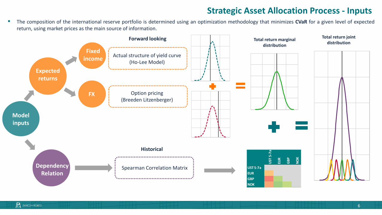
Strategic Asset Allocation Process - Inputs• The composition of the international reserve portfolio is determined using an optimization methodology that minimizes CVaR for a given level of expected

return, using market prices as the main source of information.

Modelinputs

Expectedreturns

Dependency Relation

Fixedincome

FX

Forward looking

Actual structure of yield curve(Ho-Lee Model)

Option pricing(Breeden Litzenberger)

Spearman Correlation Matrix

Total return marginal distribution

UST

5-7

a

EUR

GBP

NO

K

UST 5-7aEUR 17%

GBP 1% 60%

NOK 10% 70% 53%

Historical

Total return joint distribution

7

Implied* Distribution of Mexican Peso Annual ReturnsDensity

Source: Bank of Mexico with data from Bloomberg. * The implied distribution functions for FX, Fixed Income and Total Return securities are obtained using the Breeden-Litzenberger methodology, the Ho-Lee model, and a Copula model that combines the first two, respectively.

Implied* Distribution of Mexican Government Bonds Annual ReturnsDensity

Implied* Distribution of Mexican Government Bonds Annual Returns with FX Exposure

Density

Mean Volatility CVaRJun-14 -2.6% 9.7% 24.5%Sep-19 -4.0% 9.2% 25.3%

Mean Volatility CVaRJun-14 3.1% 4.3% 5.5%Sep-19 7.4% 4.2% 1.0%

-35% -25% -15% -5% 5% 15% 25% 35%

Jun-14 Sep-19

Mean Volatility CVaRJun-14 0.0% 9.8% 21.7%Sep-19 2.8% 9.6% 18.9%

-35% -25% -15% -5% 5% 15% 25%

Jun-14 Sep-19

-15% -10% -5% 0% 5% 10% 15% 20% 25%

Jun-14 Sep-19

7

Example: Distribution of returns of Mexican assets

-15% -10% -5% 0% 5% 10% 15%

2013

8

How do the Expected Returns Distributions of Eligible Assets Look Like?

US Dollar: Expected Distribution of Annual Returns of UST 3-5 Years Density

Source: Bank of Mexico with data from Bank of America / Merrill Lynch and Bloomberg. Non-overlapping returns.

• Expected return distributions for US dollar fixed income assets have improved significantly when compared to previous years, due to the higherlevel of interest rates and the reduction in market volatility.

-15% -10% -5% 0% 5% 10% 15%

2016 2013

8





-15% -10% -5% 0% 5% 10% 15%

2019 2016 2013

8




Expected returns in USDfixed income assetslooked more attractivein early 2019 asmonetary policynormalization in the USpushed interest rateshigher.

1


9

Distribution of Annual Returns of 3-5 Year Government Bonds in Selected CurrenciesDensity

Source: Bank of Mexico with data from Bank of America / Merrill Lynch and Bloomberg.Note: the annual return for currencies includes both government bonds income and FX returns measured in USD terms. In the particular case of CNH, the 3 month local rate return is used.

• Moreover, the distribution of US dollar fixed income returns is statistically more efficient than that of fixed income assets denominated in othercurrencies by showing higher expected returns (due to relatively higher yields in the US), and a lower variance (due to the high volatility associatedwith FX exposures).

-15% -10% -5% 0% 5% 10% 15%

UST 3-5


9



UST 3 5

-15% -10% -5% 0% 5% 10% 15%

UST 3-5 CNY



9



-15% -10% -5% 0% 5% 10% 15%

UST 3-5 CNY Gilts 3-5



-15% -10% -5% 0% 5% 10% 15%

UST 3-5 CNY Gilts 3-5 JGBs 3-5

9





-15% -10% -5% 0% 5% 10% 15%

UST 3-5 CNY Gilts 3-5 JGBs 3-5 Bunds 3-5

9




USD fixed income assetsdominate FI securitiesdenominated in othercurrencies.

2


Bills

FRN

UST

1-3

UST

3-5

UST

5-7

UST

7-1

0

UST

10-

20

UST

20-

30

EUR

GBP

CHF

JPY

Gol

d

NO

K

SEK

AUD

NZD

SGD

CNH

KRW

FRN 63%

UST 1-3 24% 0%

UST 3-5 18% -3% 95%

UST 5-7 17% -3% 89% 98%

UST 7-10 15% -3% 83% 94% 99%

UST 10-20 12% -4% 75% 87% 94% 98%

UST 20-30 10% -4% 64% 77% 85% 92% 97%

EUR 12% -2% 20% 19% 17% 14% 12% 9%

GBP 5% -3% 3% 2% 1% -1% -2% -3% 60%

CHF 16% -2% 29% 29% 26% 24% 22% 17% 86% 53%

JPY 14% 0% 43% 49% 51% 50% 47% 40% 38% 18% 49%

Gold 20% -1% 38% 41% 43% 42% 40% 35% 43% 30% 48% 51%

NOK 17% 3% 12% 11% 10% 9% 6% 4% 70% 53% 59% 70% 40%

SEK 11% 2% 9% 8% 7% 5% 2% 0% 81% 54% 27% 31% 36% 76%

AUD 9% 6% 6% 8% 9% 8% 8% 6% 42% 42% 38% 22% 39% 59% 48%

NZD 12% 0% 20% 19% 19% 18% 17% 14% 47% 40% 46% 31% 40% 52% 46% 68%

SGD 19% 6% 26% 28% 29% 27% 25% 21% 63% 50% 60% 45% 49% 65% 56% 66% 59%

CNH 5% 2% 11% 12% 11% 10% 8% 6% 37% 21% 28% 19% 27% 34% 33% 29% 29% 41%

KRW 9% 0% 12% 15% 16% 16% 14% 12% 37% 34% 33% 22% 31% 43% 36% 48% 41% 67% 28%

10

How do the Historical Relationships Between Assets are Incorporated?

Source: Bank of Mexico with data from Bank of America / Merrill Lynch and Bloomberg.Note: Spearman Correlation calculated using non-overlapping annual returns with data from 2013 to 2017

Correlation Matrix Between UST at Different Maturities and Selected CurrenciesDensity

USD Assets FX & Gold

• Correlation matrices confirm that currencies offer diversification benefits, though these are more prominent for non-traditional reserve currencies.

100.000% 100%90.000% 81%80.000% 62%50.000% 44%40.000% 25%30.000% 6%20.000% -13%10.000% -31%0.000% -50%

Non-traditionalreserve currenciesdominate traditionalreserve currencies.

3

11

How Are the Restrictions to the Model Determined?

Minimum and maximum values assined by the optimization model in different scenarios 25% -75% Range

Asset Allocation Under Different ScenariosPortfolio Weight

Source: Bank of Mexico with data from Bank of America / Merrill Lynch and Bloomberg.Note: the portfolio is optimized using historic weekly non-overlapping returns for different time periods: the dotcom crisis (2000-2002), restrictive monetary policy period in the US (2004-2007), US financial crisis (2007-2009), European sovereign debt crisis (2010-2012), as well as other periods (2015-2018, 2013-2018, 2000-2018, 2002-2004).

<- USD Assets FX & Gold ->

• To have educated restrictions set on our models, we run the optimization process under different historical scenarios (e.g. global financial crisis,European debt crisis), and see what would have been the optimal allocation under these circumstances. We then determine the minimum andmaximum allocation for each asset class to be used in the new asset allocation analysis.

0%

10%

20%

30%

40%

50%

Bills

FRN

UST

1 -

3

UST

3 -

5

UST

5 -

7

UST

7 -

10

UST

+10

0%

2%

4%

6%

8%

10%

Gol

d

EUR

GBP JP

Y

CAD

AUD

NZD

NO

K

SEK

SGD

CNH

KRW

Restrictions allow forsome discretionaryconsiderations in theSAA process (i.e.liquidity, marketstructure, traditionalreserve assets)

4

12

NEW MINDSET

WHAT IS THE RESULT?

NON-NORMAL DISTRIBUTION OF RETURNS → CODEPENDENCE

BETWEEN

ASSETS

→ EDUCATEDCONSTRAINTS→ PROSPECTIVERETURNS→ NEWOPT

IMIZ

ATIO

NM

OD

EL

-5% -3% -1% 1% 3% 5% 7% 9%

UST 3-5

13

What is the Result?

Source: Bank of Mexico with data from Bank of America / Merrill Lynch and Bloomberg.

Distribution of Non-Overlapping Annual Returns of UST 3-5 Years and the Optimized PortfolioDensity

• The portfolio´s expected distribution of returns has an attractive risk-return profile when compared to that of a UST 3-5 years exposure. In fact, thedistribution is farther right in terms of expected return, and it is also narrower (measured in terms of volatility or other left tail measures).

-5% -3% -1% 1% 3% 5% 7% 9%

UST 3-5 Portfolio

13



What is the Result?• The portfolio´s expected distribution of returns has an attractive risk-return profile when compared to that of a UST 3-5 years exposure. In fact, the

distribution is farther right in terms of expected return, and it is also narrower (measured in terms of volatility or other left tail measures).

-40%

-20%

0%

20%

40%

60%

80%

100%

120%

140%

Current portfolio Previous portfolio

Reserve CurrenciesNon-traditional Reserve CurrenciesGoldUSD Fixed IncomeMoney Markets

-5% -3% -1% 1% 3% 5% 7% 9%

UST 3-5 Portfolio

13



Contribution to CVaRPercentage

• The portfolio´s expected distribution of returns has an attractive risk-return profile when compared to that of a UST 3-5 years exposure. In fact, thedistribution is farther right in terms of expected return, and it is also narrower (measured in terms of volatility or other left tail measures).

• Moreover, given the aforementioned arguments, the bulk of our risk exposure lies within the US fixed income markets.

What is the Result?

-30.0% -20.0% -10.0% 0.0% 10.0% 20.0% 30.0%

14Source: Central Bank of Mexico

Strategic Asset Allocation Portfolios’ CompositionPercentage

Expected Return DistributionsDensity

Source: Central Bank of Mexico

• In 2019, we chose a portfolio that had a very similar left tail distribution to that of 2018´s benchmark but that was tilted to the right. This wasachieved by increasing the duration of the portfolio, by reducing gold exposure, and by reallocating risk between our basket of eligible currencies(similar USD exposure overall). We believe that the portfolio is better suited to weather the U.S. economy’s late cycle environment.

BMK 2018 BMK 2019Expected return 2.49% 2.80%

CVaR 0.82% 0.60%Duration 1.25 years 2 years

Portfolio metrics-2.0% -1.0% 0.0% 1.0% 2.0% 3.0% 4.0% 5.0% 6.0% 7.0% 8.0%

BMK 2018 BMK 2019

UST Return Range During Different Economic Stages Percentage

Recovery

Recession

Mid cycle

Late cycle

37%44%50%63%

1Y-3Y 3Y-5Y 5Y-7Y 7Y-10Y 10Y-15Y 20Y+25% to 75% return range Min and max return

Source: Central Bank of Mexico with data from Bloomberg indices. Data since Nov. 1973.

40%

50%

60%

70%

80%

90%

100%

BMK 2018 BMK 2019

Money markets UST 1-5 Y UST 5-10 Y

UST +10 Y Spread products FX spot

Non US fixed income Gold

What is the Result?

15

-25% -20% -15% -10% -5% 0% 5% 10% 15% 20%

AUD Australia 1-3 Y Australia 3-5 Y Australia 5-7 Y Australia 7-10 Y

-20% -15% -10% -5% 0% 5% 10% 15% 20%

CAD Canada 1-3 Y Canada 3-5 Y Canada 5-7 Y Canada 7-10 Y

• Our traditional approach to investing in a new currency included the use of short-term securities. Nevertheless, this year we learned that there is apowerful diversification benefit of using as an investment vehicle the long end of sovereign yield curves. Intuitively, this is attained due to the fact that- excluding a credit event - yields and FX returns are negatively correlated.

• Therefore, this year we incorporated new fixed income yield curves and reassigned our non-USD investments from the short to the long end of thecurve.

Implied Annual Returns Distribution: Canadian Dollar and Sovereign Curve Density

Implied Annual Returns Distribution: Australian Dollar and Sovereign Curve Density

Source: Central Bank of Mexico Source: Central Bank of Mexico

New Findings: A new Understanding of FX and FI risk Combined

Index

• Introduction




16

17

Distribution of Realized Weekly Returns of Optimization Strategies at Different FrequenciesDensity

• Some of the traditional SAA premises (including having a long-term approach to SAA) might not be optimal and may only be the consequence oflegacy. In this regard, we replicated our approach at different frequencies in order to gauge the impact of the investment horizon decision.

• Our finding suggests that increasing the frequency of the optimization procedure generates a strategy with a better risk-return profile. However, givenpractical issues such as transaction costs, we believe 3 months is the right spot and we are now using this tool to guide our tactical decisions.

Métricas 1M 3M 6M 9M 1Y

Mean (A) 0.04% 0.05% 0.05% 0.05% 0.05%

CVaR 95% -0.22% -0.26% -0.36% -0.41% -0.57%

Volati l i ty (B) 0.11% 0.14% 0.18% 0.21% 0.26%

Eficiency (A/B) 0.32 0.32 0.25 0.25 0.19

Source: Central Bank of Mexico with data from Bloomberg indices. To analyze the investment horizon we used non-overlapping weekly returns from 2006 and assuming independence we accumulated for 3, 6, 9 and 12 months. For each iteration, given a fixed date starting in2006, we used 5 years of historical returns to adjust the marginal probability density of each asset and to determine the maximum likelihood parameters of a t-student copula. Given the t copula parameters, we simulated 10,000 realizations of the percentiles of each asset,which were then transformed into returns with the help of each marginal density. Once we get the compounded returns for each horizon, we defined individual and group boundaries for the allocation and implement the optimization by maximizing the excess returns for afixed level of risk defined as the 95% CVaR. Finally, we evaluated the portfolio returns using the weights obtained from the optimization for the different horizons. This process was implemented for each week between 2006 and 2018.

-1.0% -0.5% 0.0% 0.5% 1.0%

1 month 3 months 6 months 9 months 1 year

New Findings: Investment Horizon

Benc

hmar

k

MBS

Gol

d

Cash

Man

ager

1

Man

ager

2

Man

ager

3

Benchmark 100%

MBS 68% 100%

Gold 60% 28% 100%

Cash 3% -2% -2% 100%

Manager 1 -58% -70% -29% -4% 100%

Manager 2 -32% -47% -13% -1% 33% 100%

Manager 3 56% 81% 28% 0% -59% -58% 100%

Absolute Return

Mandate

18

Investment Strategies Diversification - Absolute Return Portfolios•With time, we also realized that the use of benchmark portfolios to frame investment decisions could expose us to risks that we may not alwayswant to bear. For instance, a sudden increase of interest rates (normalization of term-premium).•As such, having alternative investment portfolios – not subject to a benchmark – could allow portfolio managers to focus in those strategies inwhich they have their highest conviction. In fact, they could even benefit from the normalization of interest rates through carrying negative durationin their portfolios.•With said objective in mind, we launched a pilot program of absolute return portfolios through our External Asset Management Program.

Benchmarked Strategies Non-Benchmarked Strategies• Higher flexibility. The investment decisionsdepend solely on the degree of conviction anddownside-risk management considerations

• Ability to adopt long and short positions

• Capital preservation in an environment ofhigher interest rates (particularly in UnitedStates)

• Higher returns through active management

Risk• Exposure to risk factors inherent to thebenchmark

• Dynamically allocate risk to maximize risk-adjusted return opportunities

• Portfolio's return highly correlated to thebenchmark's return

Return

Strategy DiversificationCorrelation Matrix of the Assets in the International

Reserves PortfolioPercentage

Source: Central Bank of Mexico with data from Bank of America/Merrill Lynch indices.Weekly non-overlapping returns. Data since March 2017.

Index

• Introduction




19

-40% -30% -20% -10% 0% 10% 20% 30%

2015 2016 2017 2018 2019

Date Mean Volatility CVaR 95%Jun 15 -2.0% 9.0% 23.4%Dec 16 -1.8% 9.3% 24.4%Jun 16 -3.9% 9.1% 26.0%Oct 16 -3.2% 8.9% 24.5%Dec 16 -4.9% 9.3% 26.6%Jun 17 -4.6% 9.4% 26.4%Dec 17 -4.8% 8.6% 25.7%Jun 18 -4.8% 9.1% 26.2%Dec 18 -4.3% 9.2% 26.7%Jun 19 -4.9% 8.7% 25.5%Ago 19 -4.8% 9.4% 26.7%

28

US presidential

election

• We have also used these forward-looking methodologies to enhance our market intelligence activities. In particular, to analyze our own country´sassets, to understand the perspective of international investors in Mexican securities; and to analyze the structure of the market and identifypotential opportunities and vulnerabilities.

Implied* Distribution of Mexican Peso Annual ReturnsDensity


20

Mexican Peso return distribution

-50% -40% -30% -20% -10% 0% 10% 20% 30%

Mexico Brazil Colombia Peru Chile Europe

-50% -40% -30% -20% -10% 0% 10% 20% 30%

Mexico South Africa Russia China India Europe

-50% -40% -30% -20% -10% 0% 10% 20% 30%

Mexico Poland Hungary Turkey Czech Republic Europe

-50% -40% -30% -20% -10% 0% 10% 20% 30%

Mexico South Korea Thailand Indonesia Taiwan Europe

Country Mean CVaR 95% Volatility Efficiency*

Europe 2.5% 8.5% 5.4% 2.3%Chi le -1.0% 19.2% 7.9% -1.4%Colombia -1.8% 22.0% 8.8% -2.3%Peru -2.7% 16.7% 4.9% -2.9%Brazi l -3.5% 27.6% 10.3% -4.1%Mexico -4.8% 26.7% 9.4% -5.5%


Europe 2.5% 8.5% 5.4% 2.3%China -1.0% 13.5% 5.1% -1.1%India -2.8% 16.5% 5.7% -3.0%Russ ia -4.3% 27.9% 9.2% -4.9%South Africa -4.3% 31.9% 12.2% -5.2%Mexico -4.8% 26.7% 9.4% -5.5%


Europe 2.5% 8.5% 5.4% 2.3%Hungary 2.0% 15.9% 7.7% 1.6%Poland 0.4% 16.8% 7.5% 0.1%Czech Rep 0.1% 14.3% 6.2% -0.1%Mexico -4.8% 26.7% 9.4% -5.5%Turkey -9.7% 43.6% 13.4% -11.4%


Europe 2.5% 8.5% 5.4% 2.3%Taiwan 1.0% 9.2% 4.5% 0.9%Korea 1.0% 14.0% 6.1% 0.8%Thai land 0.0% 11.3% 4.8% -0.1%Indones ia -3.7% 18.3% 6.1% -4.0%Mexico -4.8% 26.7% 9.4% -5.5%

Source: Bank of Mexico with Bloomberg data. Returns implied in one year options. Rendimientos implícitos en las opciones de mercado a un horizonte de un año* The implied distribution functions for FX, Fixed Income and Total Return securities are obtained using the Breeden-Litzenberger methodology, the Ho-Lee model, and a Copula model that combines the first two, respectively. Efficiency is measured as the expected value of the utility derived from the associated wealth at each return. The utility function is the natural log of wealth..

29

Latin America BRICS Excluding Brazil

Emerging AsiaEmerging Europe

• The methodology also allows for a comparison between different countries and offers a different perspective for the understanding of their marketstructures.

• For example, the countries with narrower densities for FX returns are usually the ones that intervene in their currency markets more actively.

Implied* Distribution of Annual Returns for Selected Currencies as of August 29, 2019Density

21

FX returns

22

Relative Efficiency of the Return Density for Selected Exchange RatesPercentage

• This process is also helpful in analyzing historical patterns, detecting regime changes, and identifying shifts in investment flows in global markets.


Historic perspective of relative efficiency: FX returns

-20% -10% 0% 10% 20% 30% 40%Brasil Colombia Perú ChileMéxico Udibonos Estados Unidos

-20% -10% 0% 10% 20% 30% 40%Sudáfrica Rusia China IndiaMéxico Udibonos Estados Unidos

-20% -10% 0% 10% 20% 30% 40%Polonia Hungría República ChecaMéxico Udibonos Estados Unidos

-20% -10% 0% 10% 20% 30% 40%Corea del Sur Tailandia Indonesia TaiwánMéxico Udibonos Estados Unidos

PaísTasa de

referenciaMedia (A)

CVaR 95% (B)

VolatilidadEficiencia

(A/B)Eficiencia

(A/C)México 8.0% 7.5% 1.2% 4.3% 6.5 1.75Udibonos 8.0% 8.0% 2.5% 5.3% 3.1 1.52Estados Unidos 2.1% 1.7% 2.1% 1.9% 0.8 0.91Bras i l 6.0% 5.4% 9.9% 7.6% 0.5 0.71Chi le 2.5% 2.1% 5.4% 3.7% 0.4 0.57Perú 2.5% 2.2% 7.0% 4.6% 0.3 0.48Colombia 4.3% 4.5% 14.8% 10.2% 0.3 0.44

PaísTasa de

referenciaMedia (A)

CVaR 95% (B)


(A/B)Eficiencia

(A/C)México 8.0% 7.5% 1.2% 4.3% 6.5 1.75Udibonos 8.0% 8.0% 2.5% 5.3% 3.1 1.52Estados Unidos 2.1% 1.7% 2.1% 1.9% 0.8 0.91R. Checa 2.0% 1.6% 3.7% 2.5% 0.4 0.62Polonia 1.5% 1.4% 3.7% 2.5% 0.4 0.54Hungría 0.9% 0.1% 5.4% 2.7% 0.0 0.02

PaísTasa de

referenciaMedia (A)

CVaR 95% (B)


(A/B)Eficiencia

(A/C)India 5.4% 5.8% 0.1% 2.8% 49.0 2.09México 8.0% 7.5% 1.2% 4.3% 6.5 1.75Udibonos 8.0% 8.0% 2.5% 5.3% 3.1 1.52Rus ia 2.5% 7.1% 2.3% 4.7% 3.0 1.49Sudáfrica 6.5% 7.3% 4.5% 6.1% 1.6 1.21Estados Unidos 2.1% 1.7% 2.1% 1.9% 0.8 0.91China 3.4% 2.8% 5.8% 4.3% 0.5 0.66

PaísTasa de

referenciaMedia (A)

CVaR 95% (B)


(A/B)Eficiencia

(A/C)México 8.0% 7.5% 1.2% 4.3% 6.5 1.75Udibonos 8.0% 8.0% 2.5% 5.3% 3.1 1.52Estados Unidos 2.1% 1.7% 2.1% 1.9% 0.8 0.91Tai landia 2.8% 1.7% 4.0% 2.8% 0.4 0.60Indones ia 4.8% 6.0% 15.5% 11.3% 0.4 0.53Corea 1.5% 1.1% 5.8% 3.4% 0.2 0.34Taiwán 1.4% 0.4% 9.1% 4.9% 0.0 0.08

23

Latinoamérica BRICS excluyendo Brasil

AsiaEuropa del este

• Local currency denominated fixed income returns show a narrower dispersion, and are usually centered on positive levels, around each country’sreference rate.


Implied* Distribution of Annual Returns in Local Currency Fixed Income for Selected Countries as of August 29, 2019Density

Local currency fixed income returns

24

• Local currency denominated fixed income returns are dominated by India and Indonesia at the beginning of the reviewed period (2015-2017), and by Mexicofrom 2017 onwards.

• It is also worth noting that there seems to be a positive relationship between expected return and volatility, as well as a gradual deterioration in relativeefficiency in developed markets.

Relative Efficiency of the Return Density for Selected Local Currency Fixed Income MarketsPercentage


Historic perspective of relative efficiency: local currency fixed income returns

-40% -30% -20% -10% 0% 10% 20% 30% 40%

Brasil Colombia Perú ChileMéxico Udibonos Estados Unidos

-40% -30% -20% -10% 0% 10% 20% 30% 40%Polonia Hungría República ChecaMéxico Udibonos Estados Unidos

-40% -30% -20% -10% 0% 10% 20% 30% 40%Corea del Sur Tailandia Indonesia TaiwanMéxico Udibonos Estados Unidos

-40% -30% -20% -10% 0% 10% 20% 30% 40%

Sudáfrica Rusia China IndiaMéxico Udibonos Estados Unidos

País Media (A)CVaR

95% (B)Volatilidad

Eficiencia (A/B)

Estados Unidos 1.7% 2.1% 1.9% 0.818Udibonos 2.7% 20.8% 10.4% 0.128México 2.5% 20.9% 10.1% 0.118Colombia 2.2% 23.3% 12.4% 0.094Bras i l 1.4% 24.0% 11.6% 0.060Chi le 0.8% 17.1% 7.9% 0.044Perú -0.5% 14.8% 6.0% -0.037

País Media (A)CVaR

95% (B)Volatilidad

Eficiencia (A/B)

Estados Unidos 1.7% 2.1% 1.9% 0.82Udibonos 2.7% 20.8% 10.4% 0.13Polonia 1.9% 14.9% 7.4% 0.12R. Checa 1.5% 12.3% 6.1% 0.12México 2.5% 20.9% 10.1% 0.12Hungría 1.8% 15.4% 7.3% 0.12

País Media (A)CVaR

95% (B)Volatilidad

Eficiencia (A/B)

Estados Unidos 1.7% 2.1% 1.9% 0.818India 2.8% 11.0% 5.7% 0.252China 1.7% 10.6% 5.4% 0.159Udibonos 2.7% 20.8% 10.4% 0.128México 2.5% 20.9% 10.1% 0.118Rus ia 2.3% 22.1% 10.1% 0.103Sudáfrica 2.7% 29.7% 15.0% 0.092

País Media (A)CVaR

95% (B)Volatilidad

Eficiencia (A/B)

Estados Unidos 1.7% 2.1% 1.9% 0.818Corea 2.0% 10.5% 5.3% 0.191Tai landia 1.6% 9.6% 4.9% 0.168Taiwán 1.3% 7.9% 4.2% 0.162Udibonos 2.7% 20.8% 10.4% 0.128México 2.5% 20.9% 10.1% 0.118Indones ia 1.8% 19.7% 10.5% 0.091

33


Asia emergenteEuropa emergente

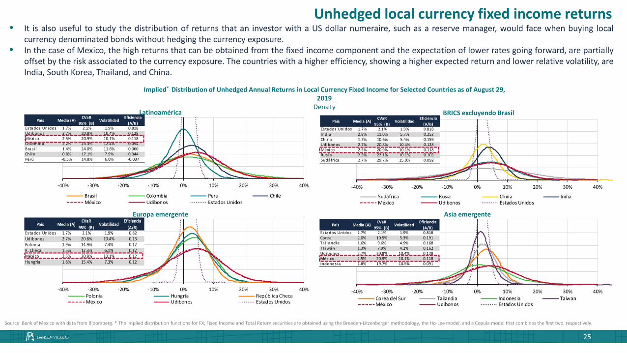
• It is also useful to study the distribution of returns that an investor with a US dollar numeraire, such as a reserve manager, would face when buying localcurrency denominated bonds without hedging the currency exposure.

• In the case of Mexico, the high returns that can be obtained from the fixed income component and the expectation of lower rates going forward, are partiallyoffset by the risk associated to the currency exposure. The countries with a higher efficiency, showing a higher expected return and lower relative volatility, areIndia, South Korea, Thailand, and China.

Implied* Distribution of Unhedged Annual Returns in Local Currency Fixed Income for Selected Countries as of August 29, 2019

Density


25

Unhedged local currency fixed income returns

26

• Our study period shows that as the Federal Reserve started its policy normalization process, the return distribution for the US becomes noticeably dominant.All the other countries also follow the US in increasing its expected returns.

Relative Efficiency of the Density of Unhedged Returns for Selected Local Currency Fixed Income MarketsPercentage


Historic perspective of relative efficiency: unhedged fixed income returns

E.E.

U.U

Euro

paR.

Uni

doCa

nadá

Suec

iaJa

pón

Aust

ralia

N. Z

elan

daM

éxico

Bras

ilCo

lom

bia

Perú

Chile

Udi

bono

sPo

loni

aHu

ngría

Sudá

frica

Rusia

R. C

heca

Chin

aM

alas

iaCo

rea

Taila

ndia

Indo

nesia

Filip

inas

Indi

aTa

iwán

Méx

icoBr

asil

Colo

mbi

aPe

rúCh

ileTu

rquí

aSu

dáfr

icaRu

siaCo

rea

Indo

nesia

Filip

inas

Taiw

án

E.E.U.UEuropa 35R. Unido 44 59Canadá 36 28 27Suecia 3 69 46 26Japón 44 45 45 21 34Australia 7 42 34 28 48 31N. Zelanda 15 46 36 4 49 34 76México -32 -4 -1 10 2 -26 17 9Brasil -18 17 1 19 18 -24 26 20 52Colombia -17 12 1 20 17 -22 3 23 6 80Perú -18 9 3 5 17 -11 31 23 66 54 56Chile -17 13 2 20 30 -23 28 3 47 9 73 51Udibonos 11 7 1 14 6 1 2 4 -1 18 19 9 3Polonia 1 15 2 29 18 1 5 30 25 35 5 40 36 4Hungría 9 28 20 43 30 15 48 65 32 34 36 43 32 13 48Sudáfrica 2 3 16 23 25 7 5 33 21 29 31 3 29 1 27 29Rusia -5 23 17 19 28 4 5 32 27 35 37 33 34 2 4 26 47R. Checa -3 14 10 2 2 1 26 3 14 21 23 19 23 9 18 14 28 36China 0 27 16 22 29 4 44 37 23 35 38 4 33 10 33 33 49 56 34Malasia 18 75 46 24 63 35 48 48 6 27 24 19 24 1 23 3 33 35 23 38Corea 17 72 43 25 61 31 46 47 8 28 24 19 25 7 21 3 32 34 20 38 9Tailandia 6 29 19 20 29 10 38 35 14 24 24 23 22 7 23 24 40 34 24 40 40 5Indonesia 8 34 26 29 35 12 53 45 22 33 34 33 31 2 31 35 50 47 32 54 46 44 53Filipinas -1 19 9 16 23 -3 38 30 26 36 37 35 34 12 32 26 42 48 28 44 35 33 38 50India 3 83 47 3 67 40 42 45 -3 17 14 12 15 5 13 25 23 25 16 28 78 73 30 32 22Taiwán 0 15 8 1 18 8 3 18 6 7 9 5 8 4 10 9 13 15 1 18 15 18 16 19 13 15México -2 19 14 4 22 9 35 30 13 18 20 15 18 13 24 16 25 26 2 27 28 25 26 30 25 23 30Brasil 3 16 12 1 19 8 4 25 9 17 18 14 16 12 21 14 19 19 18 24 22 20 25 27 3 17 32 49Colombia 9 22 16 7 23 3 35 4 6 6 7 2 6 1 2 13 15 19 18 2 24 24 23 24 19 22 25 44 36Perú -1 1 7 2 14 3 25 19 13 20 20 15 17 17 22 12 19 2 22 22 17 14 23 25 19 12 25 48 39 33Chile -1 9 9 0 13 5 23 17 9 12 14 2 9 7 16 11 2 11 15 13 17 15 15 15 13 13 22 37 37 4 35Turquía -1 14 2 4 15 8 23 2 8 14 17 9 14 1 16 13 17 16 13 19 17 16 22 24 19 13 33 5 54 25 32 33Sudáfrica 47 25 3 35 20 14 22 3 13 3 23 3 3 20 25 23 30 4 22 29 25 23 29 35 25 16 3 15 14 13 14 12 10Rusia 23 19 2 3 2 1 25 2 29 35 37 35 32 18 32 29 48 4 27 38 27 25 36 4 38 17 7 19 16 12 17 13 13 70Corea 34 26 29 32 22 12 25 23 19 26 28 28 25 17 24 24 32 34 24 4 27 25 30 35 32 17 5 18 15 15 15 12 1 79 70Indonesia 5 25 28 28 18 14 18 18 9 19 2 18 18 19 3 19 25 24 21 21 24 21 25 29 2 16 2 16 15 14 13 12 9 8 56 74Filipinas 68 28 35 36 18 20 14 17 -2 11 13 10 2 24 20 18 2 18 14 20 22 2 24 26 15 14 4 2 13 12 12 9 8 75 58 67 68Taiwán -2 6 3 15 9 -8 19 15 27 28 29 29 26 10 17 20 30 28 15 29 15 15 23 30 28 6 4 1 12 9 13 10 2 36 45 37 29 23

Emer

gent

esEm

erge

ntes

en

dóla

res

Desarrollados Emergentes Emergentes en dólares

Desa

rrol

lado

s

-25%-20%-15%-10%-5%0%5%10%15%20%25%

ene. 15 jun. 15 nov. 15 abr. 16 sep. 16 feb. 17 jul. 17 dic. 17 may. 18 oct. 18 mar. 19 ago. 19

Renta fija países emergentes Asia ex. China (3.5%) Renta fija países emergentes Europa del este (0.6%)Renta fija países emergentes Brics ex. Brasil (2.7%) Renta fija países emergentes Latinoamérica (0.1%)Renta fija países desarrollados (64.4%) Renta fija Estados Unidos (28.1%)Renta fija México (0.4%)

35Fuente: Banco de México con datos de los índices de Bloomberg. *Rendimientos semanales sin traslape (non-overlapping) anualizados. Datos de 2014-2019. La correlación de Spearman está dada por 𝜌𝜌𝑆𝑆 = 𝐶𝐶𝐶𝐶𝐶𝐶(𝐹𝐹𝑋𝑋 ,𝐹𝐹𝑌𝑌)

𝑉𝑉𝑉𝑉𝑉𝑉(𝐹𝐹𝑋𝑋) 𝑉𝑉𝑉𝑉𝑉𝑉(𝐹𝐹𝑌𝑌), mientras que la correlación lineal está definida como: 𝜌𝜌𝑃𝑃 = 𝐶𝐶𝐶𝐶𝐶𝐶(𝑋𝑋,𝑌𝑌)

𝑉𝑉𝑉𝑉𝑉𝑉(𝑋𝑋) 𝑉𝑉𝑉𝑉𝑉𝑉(𝑌𝑌)

Matriz de correlaciones de activos de renta fija de mercados globales seleccionadosPorcentaje

Correlación baja o negativa entre el mercado de renta fija de países emergentes y de países desarrollados, tanto en emisiones en dólares como en divisa local con exposición cambiaria.

Elevada correlación entre el mercado de renta fija de países emergentes con exposición cambiaria.

Correlación baja pero positiva entre las emisiones en dólares y la deuda en divisa local

Fuente: Banco de México con datos de Bloomberg. Nota: se realizó una optimización de portafolios a fin de mes en un período que comprende de enero de 2015 a agosto de 2019. 1/ Se usa el portafolio de máxima razón de eficiencia , definida como el cociente del rendimiento entre el CVaR. 2/ Se utilizó el índice Barclays Global Government Index Unhedged.

Renta fija global: evolución de la sobre/sub exposición del portafolio óptimo1/ respecto a un índice de referencia2/

Porcentaje

0.0%

1.0%

2.0%

3.0%

4.0%

ene. 15 jul. 15 ene. 16 jul. 16 ene. 17 jul. 17 ene. 18 jul. 18 ene. 19 jul. 19

Bonos M UMS Udibonos

Asignación máxima permitida para activos mexicanos de renta fija: 3.4%

• The inclusion of unhedged Emerging Market local currency fixed income assets in a global portfolio offers important diversification benefits. It is worthnoting the negative correlation of UST and JGBs with the local currency markets of Mexico, Brazil, Colombia, Perú and Chile.

• This results in a portfolio with an overweight in emerging markets and underweight in developed markets.

27

Optimal portfolio: Unhedged global local currency fixed income

-20%

-15%

-10%

-5%

0%

5%

10%

15%

20%

ene. 15 jun. 15 nov. 15 abr. 16 sep. 16 feb. 17 jul. 17 dic. 17 may. 18 oct. 18 mar. 19 ago. 19

Renta variable países emergentes Asia ex. China (3.6%) Renta variable países emergentes Europa del este (0.2%)Renta variable países emergentes BRICS ex. Brasil (4.3%) Renta variable países emergentes Latinoamérica (1.0%)Renta variable países desarrollados (33.1%) Renta variable Estados Unidos (57.5%)Renta variable México (0.3%)

36

Matriz de correlaciones de activos de renta variable de mercados globales seleccionadosPorcentaje

Fuente: Banco de México con datos de los índices de Bloomberg. *Rendimientos semanales sin traslape (non-overlapping) anualizados. Datos de 2014-2019. La correlación de Spearman está dada por 𝜌𝜌𝑆𝑆 = 𝐶𝐶𝐶𝐶𝐶𝐶(𝐹𝐹𝑋𝑋 ,𝐹𝐹𝑌𝑌)

𝑉𝑉𝑉𝑉𝑉𝑉(𝐹𝐹𝑋𝑋) 𝑉𝑉𝑉𝑉𝑉𝑉(𝐹𝐹𝑌𝑌), mientras que la correlación lineal está definida como: 𝜌𝜌𝑃𝑃 = 𝐶𝐶𝐶𝐶𝐶𝐶(𝑋𝑋,𝑌𝑌)

𝑉𝑉𝑉𝑉𝑉𝑉(𝑋𝑋) 𝑉𝑉𝑉𝑉𝑉𝑉(𝑌𝑌)Fuente: Banco de México con datos de Bloomberg. Nota: se realizó una optimización de portafolios a fin de mes en un período que comprende de enero de 2015 a agosto de 2019. 1/ Se usa el portafolio de máxima razón de eficiencia , definida como el cociente del rendimiento entre el CVaR. 2/ Se utilizo el índice MSCI global.

Renta variable global: evolución de la sobre/sub exposición del portafolio óptimo1/ respecto a un índice de referencia2/

Porcentaje

E.E.

U.U

Euro

paR.

Uni

doCa

nadá

Suec

iaJa

pón

Aust

ralia

N. Z

elan

daM

éxico

Bras

ilCh

ilePo

loni

aTu

rquí

aSu

dáfr

icaRu

siaCh

ina

Mal

asia

Core

aTa

iland

iaIn

done

siaTa

iwán

E.E.U.UEuropa 52R. Unido 6 80Canadá 66 54 56Suecia 47 9 73 51Japón -1 18 19 9 3Australia 25 35 5 40 36 4N. Zelanda 32 34 36 43 32 13 48México 24 32 33 33 32 11 29 28Brasil 21 29 31 3 29 1 27 29 53Chile 23 35 38 4 33 10 33 33 52 49Polonia 8 28 24 19 25 7 21 3 35 32 38Turquía 22 33 34 33 31 2 31 35 59 50 54 44Sudáfrica 26 36 37 35 34 12 32 26 45 42 44 33 50Rusia -3 17 14 12 15 5 13 25 23 23 28 73 32 22China 13 18 20 15 18 13 24 16 27 25 27 25 30 25 23Malasia 9 17 18 14 16 12 21 14 19 19 24 20 27 3 17 49Corea 6 6 7 2 6 1 2 13 16 15 2 24 24 19 22 44 36Tailandia 13 20 20 15 17 17 22 12 19 19 22 14 25 19 12 48 39 33Indonesia 9 12 14 2 9 7 16 11 13 2 13 15 15 13 13 37 37 4 35Taiwán 13 3 23 3 3 20 25 23 44 30 29 23 35 25 16 15 14 13 14 12

Desa

rrol

lado

sEm

erge

ntes

Desarrollados Emergentes

Correlación baja con el mercado accionario de países desarrollados

Correlación elevada y positiva con el mercado accionario de países desarrollados

• The inclusion of unhedged Emerging Market equity offers some diversification benefits.• Russia, South Korea, and Indonesia show a low correlation to developed markets while Mexican equity has a positive correlation of around 30% with developed markets.• The resulting optimal unhedged global equity portfolios show a clear tendency to overweight equity from the US, Latin America and BRICS excluding Brazil, and an underweight in other

developed markets.

28

Optimal portfolio: Unhedged equity markets

-40%

-30%

-20%

-10%

0%

10%

20%

30%

40%

ene. 15 jun. 15 nov. 15 abr. 16 sep. 16 feb. 17 jul. 17 ene. 18 jun. 18 nov. 18 abr. 19

Renta fija México (0.2%) Renta variable México (0.2%)

Renta fija Estados Unidos (10.2%) Renta variable Estados Unidos (36.6%)

Renta fija países desarrollados (23.4%) Renta variable países desarrollados (21.1%)

Renta fija países emergentes Latinoamérica (0.0%) Renta variable países emergentes (5.8%)

Renta fija países emergentes Brics ex. Brasil (1.0%) Renta fija países emergentes Europa del este (0.2%)

Renta fija países emergentes Asia ex. Asia (1.3%)

37Fuente: Banco de México con datos de Bloomberg. Nota: se realizó una optimización de portafolios a fin de mes en un período que comprende de enero de 2015 a agosto de 2019. 1/ Se usa el portafolio de máxima razón de eficiencia , definida como el cociente del rendimiento entre el CVaR. 2/ Se utilizo el índice Barclays Global Government Index Unhedged, el índice MSCI global y el índice MSCI mercados emergentes.

Evolución de la sobre/sub exposición del portafolio multi-activo global óptimo1/ respecto a un índice de referencia2/

Porcentaje

Multi-activo global: evolución de la sobre/sub exposición del portafolio óptimo1/ respecto a un índice de referencia2/

Porcentaje

0.0%

0.5%

1.0%

1.5%

2.0%

2.5%

3.0%

3.5%

ene. 15 jul. 15 ene. 16 jul. 16 ene. 17 jul. 17 ene. 18 jul. 18 ene. 19 jul. 19

Bonos M UMS Udibonos Renta variable México

Asignación máxima permitida para activos mexicanos de renta fija: 3.2%

• The optimal global multi-asset portfolio suggests an increase to fixed income markets, specifically in EM, and a lower exposure to equities.• In the case of Mexico, the model recommends a long position of Mexican assets in 36 out of the 56 months in our study. Such exposure is concentrated in

dollar denominated bonds (UMS).

29

Optimal portfolio: Unhedged global multi-asset portfolio

Final Remarks• Financial markets the last few years have posed unprecedented challenges for reserve managers, mainly because of the transition to

a more normal stance of monetary policy in the US, and the zero to negative yield environment in other developed markets.

• Banco de México has approached this new economic and financial landscape with a reassessment of the reserve managementpriorities towards capital preservation.

• In doing so, we had to reassess the way in which we analyze asset class returns, and therefore, the steps to determine our StrategicAsset Allocation. Our models have moved away from relying on historical information, into more prospective indicators that can beextracted from market prices (options and yield curves).

• Our methodology has proven useful not only to guide our SAA, but also to enhance our active management decision process. In thatregard, we have also transitioned from market-timing strategies, into more systematic trading positions.

• Finally, this methodology can also be used to assess the relative attractiveness of different assets and understand global flows froman investor perspective.

• Going forward, Banco de México will continue to evaluate and embrace methodologies that enhance the risk-return profile of itsinvestment portfolio. It will also keep a flexible approach to adapt its investment strategies to the changing conditions of financialmarkets.

30

Appendix

31

-50% -40% -30% -20% -10% 0% 10% 20% 30%

-1

0

1

2

15 20 25 30

Precio del Call

Strikes (pesos por dólar)

-1

0

1

2

15 20 25 30

Precio del Call

Strikes (pesos por dólar)

𝜕𝜕2𝑐𝑐0(𝐾𝐾)𝜕𝜕𝐾𝐾2 ≈

𝑐𝑐0 𝐾𝐾 − 𝑑𝑑 + 𝑐𝑐0 𝐾𝐾 + 𝑑𝑑 − 2𝑐𝑐0 𝐾𝐾𝑑𝑑2

METODOLOGÍA: DISTRIBUCIONES PROSPECTIVAS PARA EL RENDIMIENTO CAMBIARIO - BREEDEN LITZENBERGER

Fuente: Banco de México con datos de Bloomberg. *Rendimientos implícitos enlas opciones de mercado a un horizonte de un año al 19 de agosto de 2019. Lasdistribuciones implícitas se obtienen con base en el modelo de Ho-Lee y kernelsEpanechnikov.

Curva de volatilidad implícita en opciones del peso mexicano (USDMXN)

Porcentaje

b) Calcular la segunda derivada numérica de dicha curva respecto al strike

1 Utilizar la metodología de Breeden-Litzenberger2

a) Obtener una curva “continua” de precios de un call europeo para diferentes strikes

Distribución de rendimientos del peso mexicanoDensidad

3

Fuente: Banco de México con datos de Bloomberg.

c) Transformar a de una distribución de precios a una de rendimientos

𝒌𝒌...

𝒙𝒙...

𝒙𝒙 =𝒌𝒌𝑺𝑺𝒐𝒐

− 𝟏𝟏

𝒄𝒄𝟎𝟎 (𝑲𝑲) 𝒄𝒄𝟎𝟎 (𝑲𝑲)

Interpolacióna través de unpolinomio degrado 5

5

10

15

20

25

0 25 50 75 100

Volatilidad

Del tas

Opciones tipo callOpciones tipo put

32

33

METODOLOGÍA: DISTRIBUCIONES PROSPECTIVAS PARA EL RENDIMIENTO DE ACTIVOS DE RENTA FIJA - MODELO HO-LEE

𝑃𝑃𝑢𝑢12𝑚𝑚𝑚𝑚𝑚𝑚𝑚𝑚𝑚𝑚 = 𝑒𝑒−𝑉𝑉𝑢𝑢(𝜃𝜃1)∗𝑑𝑑𝑑𝑑[100 ∗ 0.5 + 100 ∗ 0.5]

En este proceso semestral y utilizando el bono de 12 meses, setiene que:

𝑃𝑃𝑑𝑑12𝑚𝑚𝑚𝑚𝑚𝑚𝑚𝑚𝑚𝑚 = 𝑒𝑒−𝑉𝑉𝑑𝑑(𝜃𝜃1)∗𝑑𝑑𝑑𝑑[100 ∗ 0.5 + 100 ∗ 0.5]

𝑃𝑃12 𝑚𝑚𝑚𝑚𝑚𝑚𝑚𝑚𝑚𝑚𝑚𝑚𝑑𝑑𝐶𝐶

100𝑃𝑃𝑢𝑢12 𝑚𝑚𝑚𝑚𝑚𝑚𝑚𝑚𝑚𝑚

𝑃𝑃𝑑𝑑12 𝑚𝑚𝑚𝑚𝑚𝑚𝑚𝑚𝑚𝑚100

100

Esta genera una ecuación con una incógnita a partir de la cual seobtiene �𝜽𝜽𝟏𝟏. Así, se generan los siguientes dos elementos:

𝑃𝑃12 𝑚𝑚𝑚𝑚𝑚𝑚𝑚𝑚𝑚𝑚𝑚𝑚𝑑𝑑𝐶𝐶 = 𝑒𝑒−𝑉𝑉6𝑚𝑚𝑚𝑚𝑚𝑚𝑚𝑚𝑚𝑚𝑚𝑚𝑑𝑑𝑚𝑚 𝑑𝑑𝑑𝑑[𝑃𝑃𝑢𝑢12𝑚𝑚𝑚𝑚𝑚𝑚𝑚𝑚𝑚𝑚 𝜃𝜃1 ∗ 0.5 + 𝑃𝑃𝑑𝑑12𝑚𝑚𝑚𝑚𝑚𝑚𝑚𝑚𝑚𝑚 𝜃𝜃1 ∗ 5]


𝑟𝑟6𝑚𝑚𝑚𝑚𝑚𝑚𝑚𝑚𝑚𝑚𝑚𝑚𝑑𝑑𝐶𝐶

�𝑟𝑟𝑑𝑑6𝑚𝑚𝑚𝑚𝑚𝑚𝑚𝑚𝑚𝑚

�𝑟𝑟𝑢𝑢6𝑚𝑚𝑚𝑚𝑚𝑚𝑚𝑚𝑚𝑚

�𝑃𝑃𝑢𝑢12 𝑚𝑚𝑚𝑚𝑚𝑚𝑚𝑚𝑚𝑚

�𝑃𝑃𝑑𝑑12 𝑚𝑚𝑚𝑚𝑚𝑚𝑚𝑚𝑚𝑚

100

100

100

Así, utilizando el bono de 18 meses y los resultados anteriores,se repite el proceso hasta encontrar �𝜽𝜽𝟐𝟐 y obtener:


�𝑃𝑃𝑢𝑢18 𝑚𝑚𝑚𝑚𝑚𝑚𝑚𝑚𝑚𝑚

�𝑃𝑃𝑑𝑑18 𝑚𝑚𝑚𝑚𝑚𝑚𝑚𝑚𝑚𝑚

�𝑃𝑃𝑢𝑢𝑢𝑢18 𝑚𝑚𝑚𝑚𝑚𝑚𝑚𝑚𝑚𝑚

�𝑃𝑃𝑢𝑢𝑑𝑑18 𝑚𝑚𝑚𝑚𝑚𝑚𝑚𝑚𝑚𝑚

�𝑃𝑃𝑑𝑑𝑑𝑑18 𝑚𝑚𝑚𝑚𝑚𝑚𝑚𝑚𝑚𝑚

100

100

100

100

Este proceso se repite hasta obtener �𝜽𝜽𝟑𝟑, �𝜽𝜽𝟒𝟒, … , �𝜽𝜽𝒏𝒏 ygenerar una trayectoria semestral para todas los plazosdisponibles en la curva cero y obtener un árbol neutral de latasa de corto plazo hasta el último vencimiento.

𝑟𝑟6𝑚𝑚𝑚𝑚𝑚𝑚𝑚𝑚𝑚𝑚𝑚𝑚𝑑𝑑𝐶𝐶

�𝑟𝑟𝑢𝑢6𝑚𝑚𝑚𝑚𝑚𝑚𝑚𝑚𝑚𝑚

�𝑟𝑟𝑑𝑑6𝑚𝑚𝑚𝑚𝑚𝑚𝑚𝑚𝑚𝑚

�𝑟𝑟𝑢𝑢𝑢𝑢6 𝑚𝑚𝑚𝑚𝑚𝑚𝑚𝑚𝑚𝑚

�𝑟𝑟𝑢𝑢𝑑𝑑6 𝑚𝑚𝑚𝑚𝑚𝑚𝑚𝑚𝑚𝑚

�𝑟𝑟𝑑𝑑𝑑𝑑6 𝑚𝑚𝑚𝑚𝑚𝑚𝑚𝑚𝑚𝑚

𝑞𝑞2

1 − 𝑞𝑞

(1 − 𝑞𝑞)2

1 − 𝑞𝑞 ∗ 𝑞𝑞

Las trayectorias de los procesos de cada bono son utilizadas paraobtener las distribuciones de rendimientos.

En un

Posteriormente, se asume que la curva de rendimiento dependeúnicamente de la evolución de la tasa de corto plazo, que noexisten posibilidades de arbitraje y que dicha evolución sigue unproceso binomial con la siguiente especificación:

𝑟𝑟𝑑𝑑+1𝑢𝑢 = 𝑟𝑟𝑑𝑑 + 𝜭𝜭𝑑𝑑𝑑𝑑𝑑𝑑 + 𝜎𝜎 � 𝑑𝑑𝑑𝑑

𝑟𝑟𝑑𝑑+1𝑑𝑑 = 𝑟𝑟𝑑𝑑 + 𝜭𝜭𝑑𝑑𝑑𝑑𝑑𝑑 − 𝜎𝜎 � 𝑑𝑑𝑑𝑑

𝑞𝑞

1 − 𝑞𝑞𝒓𝒓𝒕𝒕

Donde:𝒓𝒓𝒕𝒕 es la tasa libre de riesgo de corto plazo

𝒅𝒅𝒕𝒕 es el plazo en el que puede cambiar la tasa de corto plazo

𝝈𝝈 es la volatilidad de la tasa de interés de corto plazo

𝒒𝒒 es la probabilidad neutral en riesgo

Asumamos que se tiene la siguiente curva cupón cero con𝑞𝑞 = 0.5 y 𝑑𝑑𝑑𝑑 = 0.5.

Periodo Vencimiento Precio Tasa spot

t=1 6 meses 𝑃𝑃6𝑚𝑚𝑚𝑚𝑚𝑚𝑚𝑚𝑚𝑚𝑚𝑚𝑑𝑑𝐶𝐶 𝑟𝑟6𝑚𝑚𝑚𝑚𝑚𝑚𝑚𝑚𝑚𝑚

𝑚𝑚𝑑𝑑𝐶𝐶

t=2 12 meses 𝑃𝑃12 𝑚𝑚𝑚𝑚𝑚𝑚𝑚𝑚𝑚𝑚𝑚𝑚𝑑𝑑𝐶𝐶 𝑟𝑟12𝑚𝑚𝑚𝑚𝑚𝑚𝑚𝑚𝑚𝑚


t=3 18 meses 𝑃𝑃18 𝑚𝑚𝑚𝑚𝑚𝑚𝑚𝑚𝑚𝑚𝑚𝑚𝑑𝑑𝐶𝐶 𝑟𝑟18𝑚𝑚𝑚𝑚𝑚𝑚𝑚𝑚𝑚𝑚


Y que la volatilidad de la tasa de corto plazo seestima con un GARCH(1,1) , lo que genera: �𝝈𝝈

El primer paso necesario es obtener una curva cupón cerocontinua, para lo cual se ajusta el modelo de Nelson-Siegel-Svensson (NSS) a los datos de la curva de rendimiento de bonoscuponados observada en el mercado.

NSS

6.5%

7.5%

8.5%

0 5 10 15 20 25 30

Tasa de interés (%)

Vencimiento (años)

6.5%

7.5%

8.5%

0 5 10 15 20 25 30

Tasa de interés (%)

Vencimiento (años)

34

METODOLOGÍA: DISTRIBUCIONES PROSPECTIVAS PARA EL RENDIMIENTO DE ACTIVOS DE RENTA FIJA - MODELO HO-LEE

𝑉𝑉𝑎𝑎𝑎𝑎𝑎𝑎𝑟𝑟 𝑒𝑒𝑒𝑒𝑒𝑒𝑒𝑒𝑟𝑟𝑎𝑎𝑑𝑑𝑎𝑎 𝑒𝑒𝑒𝑒 𝑐𝑐𝑎𝑎𝑑𝑑𝑎𝑎 𝑒𝑒𝑛𝑛𝑛𝑛𝑒𝑒𝑎𝑎 𝑑𝑑𝑒𝑒𝑎𝑎 á𝑟𝑟𝑟𝑟𝑎𝑎𝑎𝑎 = 7.87% 7.76% 7.66% 7.56% 7.47% 7.38% 7.31% 7.23% 7.17% 7.10% 7.05% 6.99% 6.95%

...

...

...

...

...

...

...

...

...

...

...

...

7.87% 7.76% 7.66% 7.56% 7.47% 7.39% 7.31% 7.23% 7.17% 7.10% 7.05% 6.99% 6.95%

Tasa spot

Posibilidades calibradaspara la tasa de 1 mesdentro de 6 meses

Forward a 1 mes estimada de la curva cero =

Fuente: Banco de México con datos al 29 de agosto de 2019.

35

UNA PERSPECTIVA HISTÓRICA DE LA EFICIENCIA RELATIVA: RENDIMIENTO CAMBIARIO AJUSTADO CON EL TIPO DE CAMBIO FORWARD

Fuente: Banco de México con datos de Bloomberg. *Rendimientos implícitos en las opciones de mercado a un horizonte de un año con base en información mensual del 30 de enero de 2015 al 29 de agosto de 2019. Las distribuciones implícitas utilizan la metodología de Breeden-Litzenberger y kernels Epanechnikov.

Evolución de la eficiencia relativa de la distribución de los rendimientos anuales en el mercado cambiario ajustando con el tipo de cambio forward de países seleccionados

Porcentaje

• El rendimiento cambiario implícito en opciones, cuando se excluye la apreciación/depreciación asociada al tipo de cambio forward, muestra que la relación riesgo y rendimiento tieneuna pendiente cercana a cero.

• Adicionalmente, sobresale que, en el caso de México, el peso muestra un rendimiento esperado cercano a cero y un CVaR elevado en comparación con otros países de mercadosemergentes. En efecto, en los últimos meses, el peso muestra una de las razones de eficiencia más bajas de la muestra.

-60% -40% -20% 0% 20% 40% 60% 80%

México Brasil Chile Estados Unidos

-60% -40% -20% 0% 20% 40% 60% 80%México Corea del Sur Tailandia Indonesia Taiwán Estados Unidos

-60% -40% -20% 0% 20% 40% 60% 80%

México Sudáfrica Rusia China India Estados Unidos

-60% -40% -20% 0% 20% 40% 60% 80%

México Polonia Turquía Estados Unidos

País MediaCVaR 95%

Volatilidad Eficiencia*

Estados Unidos 0.3% 30.3% 14.0% -0.008Bras i l 1.8% 45.6% 23.6% -0.012Chi le -0.7% 31.2% 13.2% -0.016México -4.8% 26.5% 9.3% -0.056

País MediaCVaR 95%


India 2.4% 40.7% 22.3% -0.001Estados Unidos 0.3% 30.3% 14.0% -0.008Sudáfrica -0.2% 39.2% 19.3% -0.022China -0.8% 48.2% 20.0% -0.032México -4.8% 26.5% 9.3% -0.056Rus ia -2.8% 48.1% 24.5% -0.062

País MediaCVaR 95%


Estados Unidos 0.3% 30.3% 14.0% -0.008Polonia 0.1% 36.5% 18.6% -0.017Turquía 1.5% 45.9% 25.8% -0.020México -4.8% 26.5% 9.3% -0.056

País MediaCVaR 95%


Estados Unidos 0.3% 30.3% 14.0% -0.008Corea -0.3% 30.3% 15.0% -0.015Tai landia -1.3% 23.0% 11.5% -0.020Taiwán -2.1% 30.0% 13.0% -0.030Indones ia -1.0% 50.1% 26.1% -0.047México -4.8% 26.5% 9.3% -0.056

44Fuente: Banco de México con datos de Bloomberg. *Rendimientos implícitos en las opciones de mercado a un horizonte de un año. Las distribuciones implícitas se obtienen con base en el modelo de Breeden-Litzenberger y kernels Epanechnikov. La eficiencia está medida como el valor esperado de la utilidad de la riqueza asociada a cada elemento del soporte. La función de utilidad que se utiliza es el logaritmo natural de la riqueza.


AsiaEuropa del este

Distribución implícita en precios de mercado de los rendimientos anuales de renta variable sin cobertura cambiaria de países seleccionados al 29 de agosto de 2019 Densidad

• La distribuciones de rendimientos totales (incluyendo FX) del mercado accionario son menos homogéneas que los otros mercados, pero resalta: 1) el elevado nivel de volatilidad (muysuperior al de los otros mercados); 2) el bajo nivel de eficiencia y; 3) en muchos casos, el sesgo a observar pérdidas importantes.

• En este mercado, la distribución de México es la menos atractiva en términos de eficiencia, al tener el rendimiento esperado más bajo. Lo anterior, es probablemente el resultado delelevado nivel de correlación entre el mercado de renta variable y el peso mexicano.

RENDIMIENTO DE RENTA VARIABLE LOCAL CON EXPOSICIÓN AL TIPO DE CAMBIO

45

UNA PERSPECTIVA HISTÓRICA DE LA EFICIENCIA RELATIVA: RENDIMIENTO DE RENTA VARIABLE LOCAL CON EXPOSICIÓN AL TIPO DE CAMBIO

Fuente: Banco de México con datos de Bloomberg. *Rendimientos implícitos en las opciones de mercado a un horizonte de un año con base en información mensual del 30 de enero de 2015 al 29 de agosto de 2019. Las distribuciones implícitas utilizan la metodología de Breeden-Litzenberger, el modelo Ho-Lee y kernels Epanechnikov.

Evolución de la eficiencia relativa de la distribución de los rendimientos anuales de renta variable medidos en dólares de países seleccionados

Porcentaje

• La eficiencia relativa en el mercado de renta variable es relativamente estable a lo largo de las economías y del tiempo. Asimismo, resalta que es un mercado con niveles de volatilidadmuy elevados, en el que el riesgo y el rendimiento esperado muestran un alto grado de dinamismo en el tiempo.

• En el caso de México, resalta que, de mediados de 2016 a la fecha, el rendimiento esperado de la distribución se ubica en el nivel más bajo de la muestra. Por otra parte, el nivel de CVaRpermanece relativamente estable en un rango de entre 25% y 30%.

35

This document has been prepared exclusively for its use as supporting material for the XIII Meeting on International Reserves Management in Lima, Perú , inSeptember, 2019.

It contains confidential and privileged information that is protected by Mexican law. Partial or total reproduction, modification, use, disclosure, and/orinappropriate or unauthorized distribution of any information without the prior consent of Banco de México may be prosecuted under Mexican law. Bancode México reserves the right to pursue in any form of legal action, including any damages, that could result from the inappropriate or unauthorized use ofthe information contained herein.

strategic asset allocation models - cemla · source: bank of mexico with data from bank of america...

Documents