storm-induced risk assessment: evaluation of two tools at
TRANSCRIPT

1 Storm-induced risk assessment: evaluation of two tools at the regional and hotspot scale
2
3 Authors: O. Ferreira1, C. Viavattene2, J.A. Jiménez3, A. Bolle4, L. das Neves4, T.A. Plomaritis1, R.
4 McCall5, A.R. van Dongeren5
5
6 1CIMA/FCT, University of Algarve, Faro, Portugal, [email protected], [email protected]
7
8 2Middlesex University London, Flood Hazard Research Centre, UK, [email protected]
9
10 3Laboratori d’Enginyeria Marítima, Universitat Politècnica de Catalunya, BarcelonaTech, Spain,
12
13 4International Marine and Dredging Consultants, Antwerp, Belgium, [email protected],
15
16 5Department of Marine and Coastal Systems, Deltares, Delft, The Netherlands,
17 [email protected], [email protected]
18
19 Abstract
20
21 Coastal zones are under increasing risk as coastal hazards increase due to climate change and
22 the consequences of these also increase due to on-going economic development. To
23 effectively deal with this increased risk requires the development of validated tools to identify
24 coastal areas of higher risk and to evaluate the effectiveness of disaster risk reduction (DRR)
25 measures. This paper analyses the performance in the application of two tools which have
26 been developed in the RISC-KIT project: the regional Coastal Risk Assessment Framework
27 (CRAF) and a hotspot early warning system coupled with a decision support system (EWS/DSS).
28 The paper discusses the main achievements of the tools as well as improvements needed to
29 support their further use by the coastal community. The CRAF, a tool to identify and rank
30 hotspots of coastal risk at the regional scale, provides useful results for coastal managers and
31 stakeholders. A change over time of the hotspots location and ranking can be analysed as a
32 function of changes on coastal occupation or climate change. This tool is highly dependent on
33 the quality of available information and a major constraint to its application is the relatively
34 poor availability and accessibility of high-quality data, particularly in respect to social-economic
35 indicators, and to lesser extent the physical environment. The EWS/DSS can be used as a
36 warning system to predict potential impacts or to test the effectiveness of risk reduction
37 measures at a given hotspot. This tool provides high resolution results, but needs validation
38 against impact data, which are still scarce. The EWS/DSS tool can be improved by enhancing
39 the vulnerability relationships and detailing the receptors in each area (increasing the detail,
40 but also model simulations). The developed EWS/DSS can be adapted and extended to include
41 a greater range of conditions (including climate change), receptors, hazards and impacts,
42 enhancing disaster preparedness for effective risk reduction for further events or
43 morphological conditions. Despite these concerns, the tools assessed in this paper proved to
44 be valuable instruments for coastal management and risk reduction that can be adopted in a
45 wide range of coastal areas.

46
47 Keywords: Coastal risk; Risk assessment tools; Storm impacts.
48
49 1. Introduction
50
51 Storms impacting coastal areas are responsible for severe hazards (e.g., overwash, inundation,
52 erosion) that can lead to the destruction of goods and loss of life in occupied areas. Recent
53 examples of the above include the severe coastal erosion caused by Storm Hercules on the
54 coasts of France and England (Castelle et al., 2015; Masselink et al., 2016a,b) and the
55 associated destruction of assets; the inundation and loss of life in association with Storm
56 Xynthia in France (e.g., Garnier and Surville, 2011; Bertin et al., 2012; Vinet et al., 2012); the
57 vast destruction due to Superstorm Sandy in the Caribbean and USA (Bennington and Farmer,
58 2015; Clay et al., 2016), to Hurricane Katrina in the USA (Link, 2010; Kantha, 2013), and to
59 Typhoon Haiyan in the Philippines. Those events highlight how coastal hazards pose a
60 significant risk worldwide and can impact large cities or regions. Potential damages and risks
61 are expected to increase in the near future not only in association with climate change and sea
62 level rise, but also due to the increasing human occupation and economic development in
63 coastal areas (IPCC, 2014; Neumann et al., 2015). The development of methods for detailed
64 assessment of the risk in coastal regions and the evaluation of the effectiveness of disaster risk
65 reduction (DRR) measures is, therefore, required. The development of such tools is important
66 to prevent, or mitigate disasters; promote early warnings to stakeholders; and decide the best
67 management options with the limited resources available to coastal managers. This topic has
68 been of particular concern at the European level and funding has been awarded to projects
69 devoted to mitigating risks at coastal areas, such as the RISC-KIT project (Resilience Increasing
70 Strategies for Coasts – Toolkit; www.RISCKIT.eu).
71
72 The main goal of the RISC-KIT project was to provide such tools to the coastal community
73 (scientists, technicians, managers), at different levels (for details see Van Dongeren et al., this
74 issue). These tools include a Storm Impact Database (Ciavola, 2017; this issue) which stores
75 information on storm event impacts; a web-based management guide which documents the
76 available DRR measures (Stelljes et al., this issue); and a multi-criteria assessment to help
77 choosing the best management solutions using a participatory approach (Barquet and
78 Cumiskey, this issue). Among the developed tools two are devoted to identify the areas of
79 highest storm-induced risk and to evaluate the effectiveness of DRR measures:
80 A) The CRAF (Coastal Risk Assessment Framework; see Viavattene et al, this issue) with
81 two goals: i) hotspot identification at the regional scale (order of ~100 km); and ii) risk
82 evaluation and ranking within selected hotspots. In this paper hotspots (HS) are
83 defined as locations where risk due to extreme hydro-meteo events (e.g., storms) is
84 highest along the coast and high-resolution modelling is recommended to further
85 assess the coastal risk.
86 B) An early warning system coupled with a decision support system (EWS/DSS) with two
87 main uses: i) as an Early Warning System just prior to a storm event; and ii) as an
88 assessment tool to evaluate potential hazards and the effectiveness of DRR measures
89 well before an event.
90
91 The main goal of this paper is to critically review the performance and experience in
92 application of these two tools; to provide insights on how they should be applied; and to
93 discuss their potential, limitations and need for further improvements, based on their
94 application in ten case studies covering the European regional seas. After a summary of the
95 case studies and of the risk assessment tools, the paper presents an evaluation of the tools
96 and ends with a summary of the main application potential and restrictions to their use. For
97 specific details on the application of the tools in each case study, we refer the reader to the set
98 of case study papers in this special issue (see Van Dongeren et al., this issue).
99
100 2. Case Studies
101
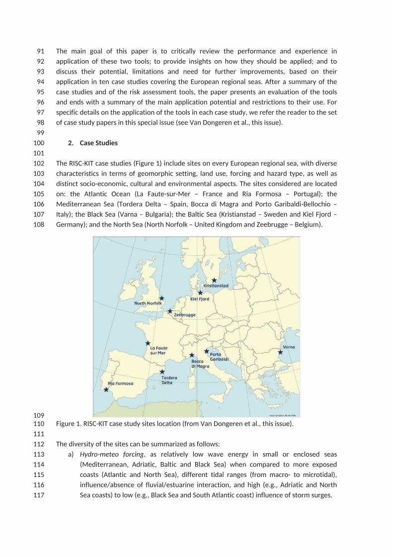
102 The RISC-KIT case studies (Figure 1) include sites on every European regional sea, with diverse
103 characteristics in terms of geomorphic setting, land use, forcing and hazard type, as well as
104 distinct socio-economic, cultural and environmental aspects. The sites considered are located
105 on: the Atlantic Ocean (La Faute-sur-Mer – France and Ria Formosa – Portugal); the
106 Mediterranean Sea (Tordera Delta – Spain, Bocca di Magra and Porto Garibaldi-Bellochio –
107 Italy); the Black Sea (Varna – Bulgaria); the Baltic Sea (Kristianstad – Sweden and Kiel Fjord –
108 Germany); and the North Sea (North Norfolk – United Kingdom and Zeebrugge – Belgium).
109
110 Figure 1. RISC-KIT case study sites location (from Van Dongeren et al., this issue).
111
112 The diversity of the sites can be summarized as follows:
113 a) Hydro-meteo forcing, as relatively low wave energy in small or enclosed seas
114 (Mediterranean, Adriatic, Baltic and Black Sea) when compared to more exposed
115 coasts (Atlantic and North Sea), different tidal ranges (from macro- to microtidal),
116 influence/absence of fluvial/estuarine interaction, and high (e.g., Adriatic and North
117 Sea coasts) to low (e.g., Black Sea and South Atlantic coast) influence of storm surges.

118 b) Geomorphic (and protection) settings, including the barrier islands of Ria Formosa, the
119 salt marshes of North Norfolk, the estuarine interaction in La Faute-sur-Mer, the fjord
120 at Kiel, the delta plain at Tordera, the highly protected coast of Zeebrugge, the open
121 and urbanized beaches of Porto Garibaldi-Bellochio and Varna, the narrow and
122 relatively sheltered beaches of Kristianstad and the embayed beaches of Bocca di
123 Magra.
124 c) Hazard type, such as coastal erosion, coastal inundation by surges or waves, overwash
125 and breaching.
126 d) Land use, as the deep-sea port of Zeebrugge, the port and town in Varna and
127 Kristianstad, the campsites in Tordera Delta, the large touristic occupation at Porto
128 Garibaldi-Bellochio and at Bocca di Magra, the natural park of Ria Formosa, the small
129 low-lying villages of La Faute-sur-Mer and North Norfolk and the marina in Kiel Fjord.
130 e) Socio-economic, cultural and environmental aspects, as the port of Zeebrugge (crucial
131 for facilitating trade and bringing significant economic benefits for the entire Belgium),
132 the North Norfolk Coast Special Area of Conservation (a Special Protection Area under
133 the Ramsar Convention), the touristic areas of Porto Garibaldi-Bellochio, Varna,
134 Tordera and Bocca di Magra (highly relevant for the regional economy), the relatively
135 local character of the Wendtorf (Kiel Fjord) marina and Praia de Faro occupation (local
136 fisherman and residents), the national relevance of a well-known liquor factory and
137 Port of Ahus exposed at Kristianstad and the unquestionable disruptive effect at La
138 Faute-sur-Mer as proved by Xynthia storm in 2010, which caused several fatalities.
139
140 The diversity of coastal types (and behaviours) expressed above makes the use of uniform
141 tools challenging. Only tools designed to be of broad use and with a high degree of
142 applicability are able to assess the risk in such a variety of environments. The RISC-KIT tools
143 have been designed in this way, with the realization that different strategies would be
144 required for some coastal areas.
145
146 3. RISC-KIT assessment tools
147
148 The Coastal Risk Assessment Framework (CRAF) is the first element of the RISC-KIT risk
149 assessment suite and is applied at a regional scale of about 100 km of coastal length. CRAF is a
150 systematic method to undertake risk assessment using simplified approaches based on simple
151 models and on a screening process to identify and rank hotspots, which may be a useful and
152 accessible instrument for most coastal managers. The CRAF provides two levels of analysis (2
153 phases).
154
155 Phase 1 (CRAF 1) is a coastal-index (CI) approach to identify potential hotspots (Figure 2, upper
156 panel). The coastal index is calculated for a uniform hazard pathway per sector of about one
157 kilometre along the coast (eq. 1 and 2).
158
159 CI = (ih * iexp)1/2 (1)
160
161
162 iexp = (iexp-LU * iexp-POP * iexp-TS * iexp-UT * iexp-BS)1/5 (2)

163
164 The hazard indicator (ih) is ranked from 0 to 5 (none, very low, low, medium, high, and very
165 high) with the null value referring to the absence of hazard. The exposure indicator (iexp)
166 embraces 5 types of exposure representative of the potential direct and indirect impacts: Land
167 Use (iexp-LU), Population (iexp-POP), Transport (iexp-TS), Critical Infrastructure (iexp-UT), and Business
168 (iexp-BS). Each is ranked from 1 to 5 (non-existent or very low, low, medium, high, and very high).
169 The overall exposure indicator (iexp) is ranked similarly from 1 to 5. The coastal index is
170 calculated separately for every hazard and return period of interest.
171
172 Phase 2 (CRAF 2) utilises a suite of more complex modelling techniques to rank the identified
173 hotspots (Figure 2, lower panel) to select the most-at-risk hotspot. Details on the CRAF
174 methodologies are given in Viavattene et al. (this issue), while this paper provides an
175 evaluation of lessons learned with the application of the tool.
176
177
178 Figure 2. CRAF overview and required steps, as a vertical top-down sequence of analysis,
179 resulting in hotspot identification (A, B and C in the upper panel) and ranking (A > C > B, in the
180 lower panel).
181

182 The Early Warning System and Decision Support System (EWS/DSS) makes use of complex-
183 modelling techniques (2DH – two-dimensional horizontal process-based, multi-hazard
184 morphodynamic model, Bayesian Network (BN) analysis) and the demand in terms of data,
185 time and resources is subsequently greater than that for the CRAF. The EWS/DSS (Bogaard et
186 al., 2016; Jäger et al., this issue) is built using the Delft-FEWS software environment (Werner et
187 al., 2013; De Kleermaeker et al., 2015). The philosophy of the system is to provide an open
188 shell for managing data handling and forecasting processes. This system can be organized
189 using the following structure (see Figure 3): data import from external sources (i.e., NOAA GFS,
190 local meteorology, measurement stations); data processing; model runs (WaveWatchIII,
191 Delft3D, Telemac, XBeach); data post-processing; and export to external processes (BN and
192 web viewer). The Bayesian Network is in essence a probabilistic graphical model, which
193 consists of random variables (e.g., wave characteristics, water level, hazard intensity, exposed
194 elements) and conditional dependencies (obtained from modelling approaches or
195 observations) between those variables (Poelhekke et al., 2016). The Bayesian-based Decision
196 Support System integrates hazards and socio -economic, cultural and environmental
197 consequences. These systems can be built as stand-alone applications, run manually by a user,
198 or they can be transformed into fully automated systems.
199
200
201 Figure 3. Schematic of the Delft-FEWS concept applied to the RISC-KIT EWS framework. The
202 demanding computational part is performed within the Delft-FEWS system. A visualisation
203 interface is then required (e.g., FEWS controller, or web viewer). WMS – Web Map Service.
204
205 In addition to providing forecasts of storm impacts, the EWS/DSS tool can be used to assess
206 the effectiveness of potential DRR measures. In the RISC-KIT project these were chosen by
207 expert judgment in consultation with end-users and stakeholders, and by using information
208 from existing management plans. The impact of predicted future climates scenarios (e.g., sea
209 level rise and extreme storm surge levels), based on available projections at the regional scale
210 under the Representative Concentration Pathway 8.5 or other adequate estimate, were
211 incorporated in the performed tests and afterwards in the EWS/DSS systems to assist in the
212 assessment of the future effectiveness of DRR measures.
213
214 4. Coastal Risk assessment Framework (CRAF)
215
216 4.1 CRAF 1
217
218 CRAF 1 is a coastal-index approach to identify potential hotspots (Figure 2, upper panel)
219 subject to hazards such as: Flooding/Inundation (see as examples Armaroli and Duo, this issue;
220 Christie et al., this issue; Jiménez et al., this issue), Erosion (see as examples Armaroli and Duo,
221 this issue; De Angeli et al., this issue; Jiménez et al., this issue), Overwash (see as examples
222 Ferreira et al., 2016; Valchev et al., 2016) and Breaching (see Plomaritis et al., this issue(b)).
223
224 4.1.1 Hazard assessment
225
226 Event versus Response approach
227
228 Because storm-induced coastal hazards usually depend on more than one variable (e.g., water
229 level, wave height or storm duration), which are not necessarily correlated, we recommend to
230 adopt the response approach (Divory and McDougal, 2006; Bosom and Jiménez, 2011; Garrity
231 et al., 2012) to assess those hazards. The response approach uses the forcing (wave and water
232 level) time series to derive a time record of the onshore hazard parameter (e.g., wave run-up,
233 total water level, overtopping, eroded volume), which is then fitted to an extreme value
234 probability distribution. This allows the hazard magnitude associated with a given probability
235 of occurrence to be obtained without assuming relationships between driving variables,
236 thereby reducing uncertainty in the analysis. The application of such an approach requires
237 access to the forcing data (wave characteristics and water levels) and to have long-term data
238 sets of those variables to perform a reliable analysis of extremes. If such datasets do not exist
239 or are not available, the event approach can be used. In this case, the probability of occurrence
240 of the event can be computed by using: i) a single variable (e.g., wave height); ii) a joint
241 probability of variables; or, as often is used iii) empirical relationships between different
242 variables (e.g., period and/or storm duration versus wave height). The obtained value(s) are
243 then used to compute the hazard magnitude for a given return period, assuming that the
244 hazard probability of occurrence is equal to the hazard probability of the event. However, due
245 to the multiple inter-dependences, it is likely that more than one event can produce the same
246 hazard magnitude and, thus, this approach constitutes a simplification that may lead to
247 underestimation (e.g., if only the annual maximum event is considered for the return period
248 definition) or overestimation (e.g., if the interdependencies between variables are not
249 accounted for in the statistical analysis).
250
251 Suggested formulations/methods
252
253 One of the advantages of the method developed in the CRAF is that, at the regional level, the
254 assessment can be done by using simple formulations/equations (e.g., run-up formulations,
255 simple storm driven erosion models) and approaches (e.g., bathtub, overwash extent and

256 depth, flood depth) which are easy to implement (Table 1). Moreover, the CRAF 1 is flexible
257 enough and can be adapted to incorporate different assessments and methods that are
258 already in use at some locations (cf., Armaroli and Duo, this issue; De Angeli et al., this issue).
259 In cases where the local characteristics do not allow a proper definition of the hazard
260 magnitude by using simple approaches, the proposed methods need to be adapted prior to
261 their application (e.g., Ferreira et al., 2016; Christie et al., this issue). One example is the
262 analysis of flooding in extensive low-lying areas (e.g., Belgian Coast; Ferreira et al., 2016),
263 where the bathtub approach would substantially overpredict the flood prone area. In such
264 cases, a simple flood model should be used instead, or some low hinterland areas must be
265 excluded prior to the flood analysis. In areas with large alongshore tidal range variations, or
266 with extensive saltmarshes (e.g., North Norfolk; Christie et al., this issue) adaptations to the
267 proposed methodology (e.g., alongshore variation of sea levels and hazard reduction by salt
268 marshes) should also be implemented. Overall, the methodology is efficient to properly assess
269 storm-induced hazards at the regional scale for most sedimentary coasts. Moreover, it is
270 flexible enough to be adapted (and modifiable), when local coastal characteristics make the
271 application of simple tools an impractical exercise.
272
273 Table 1: Proposed methods for assessing hazard intensities and extent.
Hazard Methods Outputs
Overwash Holman (1986), Stockdon et al. (2006)(a) Run-up level
Overwash
extent
Simplified Donnelly (2008), XBeach 1D
(Roelvink et al., 2009)
Water depth, velocity and/or extent
Overtopping Hedges and Reis (1998), EurOtop (Pullen et
al., 2007)
Run-up level and/or discharge
Inundation Bathtub approach, fast 2D flood solver (e.g.,
LISFLOOD-FP; Bates and De Roo, 2000)
Flood depth, velocity
Storm
Erosion
Kriebel and Dean (1993), Mendoza and
Jiménez (2006), XBeach 1D (Roelvink et al.,
2009)
Eroded volume, shoreline retreat
and/or depth
274 (a) For the wave run-up calculation
275
276 Hazard extent
277
278 The definition of the hazard extent, the inland area influenced by the hazard per sector for a
279 given return period, is the basis of the impact assessment. The exposure indicators are applied
280 to a given hazard extent and, depending on the elements exposed to the hazard within that
281 extent, the final coastal-index value can be different. The following hazard extents can be
282 considered:
283 i) Flooding/Inundation (sometimes including overwash)
284 It is recommended to use a method in CRAF 1 that derives a flood-prone area based on
285 physical principles. A simple method to define the extent is the bathtub, or a tilted bathtub,
286 approach applied to the total water level or to the overwash level. A simple 2D model can also
287 be used to define the hazard extent (cf. Ferreira et al., 2016). Alternative methods include an
288 arbitrary extent of X m (buffer zone), based on local evidences, or the surface area of the
289 municipality to be flooded.
290 ii) Erosion

291 The recommended hazard extent to be used is a buffer zone with a given distance from the
292 shoreline/dune line, derived from the maximum computed shoreline retreat. In some cases
293 this buffer zone can be replaced by a representative extent based on expert judgment and
294 historical analysis (variable from place to place).
295 iii) Overwash
296 Where possible, it is recommended to use the overwash extent developed by Plomaritis et al
297 (this issue(b)), an adaptation of Donnelly’s formulation (Donnelly, 2008; Donnelly et al., 2009).
298 In the absence of sufficient data for this method, the spit width or an arbitrary inland extent
299 (based on expert judgment) can be used.
300 iv) Breaching
301 The methodology developed by Plomaritis et al (this issue(b)) is recommended for use to
302 assess breaching and the associated extent (related to the flood delta width).
303
304 Hazard Indicators
305
306 Application of the CRAF during the RISC-KIT project has shown that various indicators exist for
307 similar hazards, that the appropriateness of indicators depends on the specificities of the
308 coastal region, and that it is not simple to find universal indicators that can be easily applied at
309 coastal areas with different morphologies. A synthesis of suggested indicators per hazard is
310 provided below.
311
312 Flooding/Inundation
313 Indicators to assess this hazard include: Flood depth; Percentage of overtopping flooded area;
314 Total water level; Overtopping discharge; and Flood extension. Some just represent the hazard
315 process (overtopping discharge or total water level) while others relate the hazard to the
316 affected area (flood depth, percentage of flooded area, flood extent). The use of an impact-
317 related indicator is recommended since it integrates the hazard and the coastal morphology
318 while one that only incorporates changes on the hazard may not be useful along coasts with
319 high morphological variability. Simple indicators like flood depth are, therefore,
320 recommended.
321
322 Overwash
323 Overwash depth (Od) (see Donnelly et al., 2009) and Overwash potential (Op) (see Matias et
324 al., 2012) are conceptually similar indicators that express a vertical difference between the
325 overwash level over the dune crest (Od) or the maximum potential run-up level (Op) against
326 the dune/barrier crest. Op is used for its simplicity of computation while Od is more accurate
327 in terms of the actual process. Both indicators are recommended for further use.
328
329 Erosion
330 Erosion assessment was related with episodic storm driven erosion and not structural erosion.
331 Commonly used indicators include: Shoreline retreat; Dune retreat; Berm retreat; and
332 Remaining beach width. These indicators can be reduced to two (shoreline/berm retreat and
333 dune retreat). The use of dune retreat versus berm retreat depends on the exposure to be
334 assessed. For coastal sites with infrastructures located on the beach berm (e.g., bars,
335 amenities), the berm or the shoreline retreat should be used. This can then be transformed (or

336 not) into a remaining beach width or a distance to occupation. For coastal areas where
337 infrastructure is located on the dune or in the hinterland, the dune retreat should be used.
338 This can also be transformed into a remaining distance to occupation.
339
340 Breaching
341 Available breaching information is largely qualitative (Kraus, 2003) and there are only few
342 methods devoted to determine or rank breaching vulnerability. Kraus et al. (2002) proposed a
343 breaching susceptibility index based on the ratio between the 10 year surge return period and
344 the tidal range, but this method does not include any morphological characteristics. Basco and
345 Shin (1999) proposed the use of a series of numerical models to separately evaluate overwash
346 and erosion processes. Plomaritis et al. (this issue(b)) developed a new indicator (Breaching
347 Potential) which integrates parameters such as overwash, structural erosion, storm erosion,
348 subaerial barrier volume, back barrier depth and morphology, and washover width to barrier
349 width ratio. This parameter is recommended for further use.
350
351 4.1.2 Exposure Assessment
352
353 The hazard indicators described above are combined with exposure indicators to obtain a final
354 coastal index to identify potential hotspots.
355
356 Land Use
357 For this indicator CORINE Land Cover (CLC; http://www.eea.europa.eu/publications/COR0-
358 landcover) data can be used as the source to characterise land use data. CLC can, however, be
359 replaced if a better and more detailed cartography is available, allowing a more detailed
360 evaluation of the land use indicator per sector. CLC is also not very useful for some hazards,
361 namely overwash and erosion, since the extent is too narrow (tens of metres) to be captured
362 by the CLC resolution. Overall, it is recommended to use the most detailed land use
363 cartography provided by national, regional or local authorities, or to produce one when not
364 available. That is particularly relevant for small hazard extents bordering the coastline (e.g.,
365 erosion or overwash). Stakeholder involvement is recommended for valuing land use.
366 Alternatively existing valuations or user judgment can also be applied.
367
368 Population and social vulnerability
369 An SVI (Social Vulnerability Indicator) is applied to characterise the potential non-tangible
370 impacts to the population. Two main options are recommended: The first uses an existing SVI
371 for the region. The second one consists on developing a specific SVI for the area following the
372 CRAF 1 methodology guidance (see Viavattene et al., this issue) using census data. The “age of
373 the population” characteristic and the financial deprivation are fundamental parameters to
374 calculate the SVI for most regions. A third main important characteristic is education. Health
375 can also be included when relevant. In general, it is relatively simple to build a specific SVI
376 when needed, allowing the method to be applicable to a broad range of conditions.
377
378 Transport systems
379 National or local transport maps should be used to define the transport network, in absence of
380 which OpenStreetMap data can also be used as a source of information. The valuation (see
381 Viavattene et al., this issue) is straightforward since it is based on the classification system of
382 the roads obtained from the map, matching the descriptive scale proposed in the CRAF
383 methodology (from local to national and highway roads). Information on other transports
384 (trains, ports, and airports) or relevant local knowledge on the importance of local roads can
385 also be used in the valuation. In most coastal areas moderate values are expected to dominate
386 the assessment except for the widely urbanised coasts (cf. Ferreira et al., 2016; Jiménez et al.,
387 this issue).
388
389 Utilities
390 The CRAF assessment method is simple and uses a ranking table for utilities. The approach is
391 limited by the availability of information on the location of receptors, and the valuation is
392 therefore often based on expert judgment. In most coastal areas, very low to moderate values
393 are expected to dominate the assessment except for widely urbanised coasts.
394
395 Business Settings
396 The business settings indicator consists of a simple table with criteria to distinguish between
397 different types of businesses and how to rank them. The table can be adapted in order to
398 better relate to the specific business type/setting of each considered coastal area. In highly
399 touristic areas (e.g., the Emilia-Romagna coast discussed in Armaroli and Duo, this issue; and
400 the Catalan coast in Jiménez et al., this issue) the indicator can be adapted to a tourist-based
401 index (as a proxy for existing facilities). Even when case-specific adjustments are required, the
402 method is simple to implement. The involvement of stakeholders is essential to validate the
403 valuation.
404
405 4.1.3 Coastal Index (CI)
406
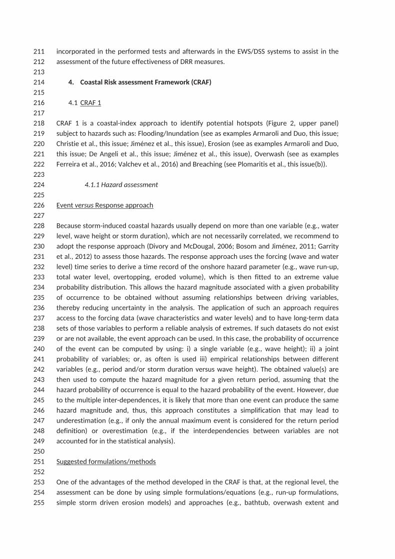
407 The CI is a measure for the combined hazard and exposure in a given sector (see Ferreira et al.,
408 2016 and Viavattene et al., this issue), and is used to identify potential HS. An example of the
409 final application of a CI along a coastal zone using sectors of about 1 km is presented in Figure
410 4.
411
412

413 Figure 4. CI applied to the Ria Formosa (Southern Portugal) for overwash and a return period
414 of 50 years, with the identification of 2 main hotspots.
415
416 Return period
417 When defining the storm-induced hotspot, a relevant issue is the definition of its “severity”.
418 This is done through the selection of a return period for the analysis. More than one return
419 period can be (and should be) computed for the same coastal area. This allows an evaluation
420 of possible HS changes according to the return period used within each coastal area. The
421 chosen return periods will vary from site to site, depending on the return periods already in
422 use for coastal management, and their selection should be agreed with local stakeholders.
423 While in some countries (e.g., Portugal) return periods of 100 years are not yet (or rarely)
424 considered, on highly protected coasts (e.g., Belgium) return periods greater than 1000 years
425 are increasingly common in coastal management and safety plans. The selection of return
426 periods in the CRAF 1 should be discussed with stakeholders and reflect their needs or
427 recommendations. The relatively limited number of years (few decades) of available measured
428 or hindcast data reduces the ability to produce results with a high degree of accuracy for large
429 return periods (hundreds to thousands of years), which is still a drawback of the CRAF
430 methodology, as for any other. On the other hand, this method permits results with a high
431 degree of confidence for lower return periods (<100 years), which are most commonly used by
432 the majority of coastal managers and end-users.
433
434 Potential Hotspot identification
435 The number of potential HS determined in CRAF 1 depends not only on the models and scoring
436 applied in the analysis, but also on the chosen return periods, since both the hazard and the
437 exposure will change with the return period. Using a very small return period (e.g., in the order
438 of one to a few years) will probably lead to a small number of HS (due to no or very restricted
439 hazard), while using a very large return period (>1000 years) can lead (mainly at unprotected
440 coasts) to numerous HS, with a difficulty in selecting or ranking among them. This reinforces
441 the need to analyse several return periods for each coastal area in order to better choose the
442 most relevant one, in consultation with the relevant stakeholder (e.g., coastal manager). To
443 reduce the possibility of having false negatives, it is advised to consider a worst case geometry
444 (i.e., a profile with a lower dune/elevation) as a representative coastal profile rather than an
445 alongshore-average profile. In some cases, coastal sectors may require a higher resolution (< 1
446 km), since they may include (within the 1 km) different morphologies (e.g., relevant
447 differences in dune height or berm width). Changes in coastal morphology, occupation and
448 management will lead to relevant shifts in risk over time requiring a reapplication of the
449 method.
450
451 Hotspot validation
452 A validation of the obtained CI should be performed after CRAF 1 application (as an example of
453 application see Armaroli and Duo, this issue; Figure 5). The sources to be used for validation
454 include historical information on damages, comparison of results against existing evaluation
455 methods, field measurements of storm damages and hazards, and stakeholder information.
456 The use of historical records as a source of validation must be performed with care since past
457 events/consequences may not be representative of present day conditions. For instance, the
458 improvement of coastal protection works taking into consideration longer return periods and
459 tighter safety conditions (e.g., the Belgian coast) disable the use of historical analysis for
460 current conditions. The same applies when relevant land use changes (e.g., house removal,
461 restoration of saltmarshes) have been implemented. Potential deviations between
462 observations and CRAF 1 results can be associated to the following factors:
463 i) The available data and the analysis do not consider recent coastal management
464 protection in place and therefore the HS highlighted do not completely represent
465 current conditions;
466 ii) A limitation of the CRAF 1 methodology in not capturing the bi-dimensional hazard
467 pathways (e.g., hydraulic interconnectivity);
468 iii) CRAF 1 simplification of complex coastal morphologies by just using one profile per
469 sector (average or worst case), which does not completely represent the
470 behaviour of the sector.
471
472 CRAF 1 permits the identification of HS existing at a high variety of coastal zones with different
473 morphologies and degrees/types of occupation (cf. Armaroli and Duo, this issue; Christie et al.,
474 this issue; De Angeli et al., this issue; Ferreira et al., 2016; Jiménez et al., this issue; Plomaritis
475 et al., this issue(b); Valchev et al., 2016). The CI for a given region can be recalculated by
476 incorporating new data or regional DRR actions, defining in what way (and by what amount)
477 the HS will be affected. This allows the assessment of the evolution of the HS as a function of
478 coastal evolution, but also of coastal management interventions. CRAF 1 has inherent
479 limitations since it uses simple approaches, formulations, databases, and indicators to assess
480 complex coastal problems for a high diversity of coastal types, including areas with important
481 morphological complexity. Therefore, for some cases (e.g., extensive interconnected low-lying
482 areas or complex alongshore morphologies) the method is too simple and the formulations
483 may not apply. The assumptions used in the CRAF 1 methodology can then result in over- or
484 underestimation of the coastal risk. In such case it is recommended to increase the number of
485 hotspots to be analysed in Phase 2, where more complex and robust models are used.
486

487
488 Figure 5. Example of validation of the critical sectors at Emilia-Romagna (from Armaroli and
489 Duo, this issue) against historical data for flooding (left panel, A) and erosion (right panel, B).
490
491 4.2 CRAF 2
492
493 Once potential HS are identified with CRAF 1, the next step (CRAF 2) consists of an in-depth
494 analysis to discriminate the potential HS in terms of potential impacts by using advanced
495 modelling. This section discusses the applicability of CRAF 2, including results achieved,
496 difficulties identified, and adaptations made, as well as constraints to its application and usage.
497 It also presents recommendations for the application and improvement of the tool. The
498 analysis is split in three sub-sections regarding Hazard and Impact assessments, and hotspot
499 ranking.
500
501 4.2.1 Hazard assessment
502
503 As for CRAF 1, we recommend the use of the response approach in CRAF 2 to compute return
504 periods of local hazards (flooding and erosion). The recommended models to determine the
505 hazard associated with episodic erosion and/or flooding are the open-source process-based
506 nearshore storm impact model XBeach (Roelvink et al, 2009; for erosion) or XBeach coupled
507 with the overland flood model LISFLOOD-FP (Bates and De Roo, 2000; for marine flooding),
508 with XBeach providing the discharges at the top of the dune/breakwater and LISFLOOD-FP
509 distributing the amount of water along a given area (Viavattene et al., this issue). In both cases
510 XBeach is run in simplified 1D cross-shore profile mode to reduce computational requirements
511 and allow for large sections of the coast to be analysed. Note that other models and
512 approaches can be used, and these can be tailored to the specific geomorphological and
513 hydrodynamic setting. The methodology to assess the hazard discussed in this paper (1D
514 XBeach coupled with LISFLOOD-FP) is relatively easy to apply on a vast number of diverse

515 coastal areas, and has the benefit of relying on models with an extensive user and validation
516 base, providing some confidence in their application in cases with limited validation data. The
517 spatial distribution of the hazard is simulated by using topographic grids, normally of high
518 resolution. Grids on the order of 1x1 m to 10x10 m seem to be able to fully represent the
519 properties of the hazard. Some of the modelling limitations include the lack of high-quality
520 quantitative validation for both XBeach and LISFLOOD-FP models due to lack of data,
521 particularly relating to water discharge, water velocities and inundation extent.
522
523 4.2.2 Impact assessment
524
525 The INDRA (Integrated Disruption Assessment Model; see Viavattene et al., 2017; this issue) is
526 capable of assessing eight receptor-related impact indicators: household displacement,
527 household financial recovery, regional business disruption, business financial recovery,
528 ecosystem recovery, risk to life, regional utilities service disruption and regional transport
529 service disruption. This section reviews the potential for INDRA application and proposes
530 recommendations for future use.
531
532 Data quality
533 The potential problem of lack of data was foreseen and the CRAF 2 was set up to allow for
534 assessments in data-poor or data-rich contexts, as well as to help identify and report data
535 limitations and provide recommendations on improving data collection. To better assess data
536 limitation a Data Quality Score DQS (Table 2) is recommended to be applied to all coastal areas
537 as a self-evaluation of data quality and required improvements.
538
539 Risk to life, household displacement and both household and business financial recovery are
540 the most relevant indicators for impact assessment. Other indicators may or may not be
541 considered if they are significantly (or not) exposed to the hazard. Data of sufficient quality are
542 often lacking (see Viavattene, this issue), and even at the European case-study sites of the
543 RISC-KIT project DQS of 2 or 3 are most common. Data quality will then be site-specific and
544 often dependent on the availability of research surveys. Data availability and data quality are
545 therefore pressing problems and require an improvement either promoted specifically for the
546 needs of the local and regional authorities, or developed as standardized data by national and
547 European authorities.
548
549 Table 2. Data Quality Score
550
551 Land use data and vulnerability indicator
1 Data available and of sufficient quality for CRAF 2.
2 Data available but with known deficiencies. Improvements required in the
future
3 No data available/poor data use of generic data but representative enough.
New data will be required.
4 No data available/poor data, use of generic data but likely not representative.
New data will be required.
5 No data available, based on multiple assumptions

552 Information on the geographic location of receptors and their type is essential to calculate
553 direct impact. Land use data are often available (national, regional or municipal dataset)
554 allowing an exact representation of the geographic location of receptors. However,
555 information on the type of receptors (buildings type and associated activity) is limited,
556 requiring additional survey (local, satellite, online). The vulnerability indicator to assess the
557 direct impacts in INDRA can be derived from country-specific datasets or generic datasets.
558 National vulnerability indicators for depth-damages curves are only available in a few countries
559 (e.g., France, Belgium, UK). Where this information is not available, generic data or peer-
560 reviewed papers should be used to generate vulnerability indicators, but confidence in the
561 quality of these indicators is limited. Research is therefore still needed at national and
562 European level to better determine representative vulnerability indicators.
563
564 Household displacement
565 The displacement of, and subsequent disruption to, households is linked in the model to the
566 direct impacts to residential buildings due to flooding and erosion. The approach requires the
567 user to reflect on different displacement durations experienced by households for different
568 hazard intensities using ex-ante or post surveys. The information to assess household
569 displacements is, however, very scarce, and generic data or limited post-event information are
570 then used. Confidence in using the poorly-available post-event data is limited since these are
571 generally not found in peer-reviewed publications or official reports, but in media reports.
572
573 Financial recovery (household and business)
574 The assessment of the financial recovery requires distributing the number of properties across
575 different recovery mechanisms: no insurance, self-insured, small government compensation,
576 large government compensation, partly insured, fully insured, for households; and no
577 insurance, self-insured as large corporate business, self-insured with access to resources,
578 state-owned, partly insured, fully insured, for businesses. Values for financial recovery can be
579 based on national policies, however a differentiation in sub-regions is recommended. There is
580 currently a clear lack of data to distinguish local and regional differences. Access to insurance
581 data and interviews may provide such information – preferentially including a geographic
582 differentiation of the financial recovery distribution within the region.
583
584 Transport and utility disruption
585 The assessment of transport disruption requires the mapping of the regional transport
586 network and the importance of locations within the network. Mapping road networks is often
587 simple. Categorizing road transport capacity (associated with the speed limit) could be
588 achieved using road typology. The importance of junctions can be included, mainly based on
589 the type of road (flow and service associated with importance) and on the presence of specific
590 services identified near the junction (e.g., hospitals, commercial areas). In contrast, mapping
591 and categorizing utility networks is often hampered by limited public data availability and
592 assessment of impacts to these networks often require a direct input from stakeholders in the
593 utilities sector.
594
595 Business disruption

596 Business supply chain disruption considers the potential impacts on the economy, including
597 the tourism economy. For the later, the assessment can be driven by the potential loss of
598 attractiveness (beach) and the loss of accommodation, seasonality being an important factor
599 to address (time laps between storm impacts and start of the tourist season). The impacts on
600 harbour activities (e.g., loss of warehousing facilities) and the transport of goods are other
601 examples to be evaluated under this indicator. Two components are key to assessing the
602 business disruption: the reinstatement time and the business supply chain. If there is no
603 information on business recovery for a given coastal area, generic data can be used as default
604 values. The use of generic data can be considered a critical problem, as it has serious
605 implications in the supply chain calculation, in particular when seasonality has to be
606 considered. The lack of data can result in very simplified supply chains limited to two or three
607 tiers. Engagement with business-related stakeholders, surveys and the involvement of experts
608 in market or economic research will be beneficial for future assessments of this kind.
609
610 4.2.3 Hotspot ranking
611
612 A MCA (multi criteria analysis) is applied in CRAF 2 to weight the different indicators in each
613 coastal area, allowing a comparison between selected HS (see Viavattene et al., this issue). The
614 weighting for the MCA is either based on experts’ or stakeholders’ inputs. Multiple MCA
615 weights can be tested, to represent different perspectives. It is advisable to have a good
616 involvement with stakeholders to better define the weights of each indicator (cf. Christie et al.,
617 this issue; and Table 3).
618
619 Confidence in the impact assessment varies as a function of data quality. However, the
620 approach combining simplified indicators and generic data allows the user to perform a first
621 impact assessment and, in discussion with their stakeholders, to investigate which elements
622 need essential improvement and consider options for improving their dataset as well as
623 agreeing on the HS. It may be noted that in some cases an agreement on the selected hotspot
624 may not be achieved. This may happen if differences in stakeholder perspective lead to
625 strongly different results during the MCA. The contribution of the various indicators to the
626 total score may also vary between HS. If similar impacts are analysed at all HS, then limitations
627 in data quality, and differences in the indicator assessment and MCA weighting are similar
628 across the HS and therefore have less influence in their comparative assessment.
629
630 Table 3. Example of MCA (multi criteria analysis) application and final CRAF 2 scores for two
631 hotspots from the North Norfolk coast (UK). Method A - neutral approach; Method B - expert
632 judgement where people, households and business are highlighted; Method C - expert
633 judgement where people and ecosystems are highlighted (for details see Christie et al., this
634 issue). Higher values represent potentially higher consequences, for the same considered
635 hazard. It is relevant to note that the most important hotspot can change as a function of the
636 chosen indicators weight.
Indicators MCA weights (%) per method
A B C
Risk To Life 12.5 30 35
Household Financial Recovery 12.5 10 5

Household Displacement 12.5 15 5
Business Financial Recovery 12.5 15 5
Business Disruption 12.5 10 5
Natural Ecosystem 12.5 5 20
Agriculture 12.5 5 5
Transport disruption 12.5 10 20
Wells-next-the-Sea Score 0.1243 0.1053 0.1594
Brancaster Score 0.1880 0.0790 0.2825
637
638 5. Early-Warning System/Decision Support System (EWS/DSS)
639
640 The EWS/DSS is a tool to be used at the hotspot that is selected using the CRAF method. The
641 EWS/DSS can be used both to provide forecasts of storm impacts as well as to assess the
642 effectiveness of the DRR measures in the planning stage. The main types of hazards to be
643 considered are marine flooding, overwash, and episodic (storm induced) erosion. The results
644 of the high-resolution hazard models are translated into impact using damage curves or any
645 other relationship that relates hazard into damage of the receptors. The associated hazard and
646 impact information is stored in a self-learning Bayesian Network (BN).
647
648 5.1 The model train
649
650 The coastal Delft-FEWS system (Bogaard et al., 2016) is recommended to be used as a common
651 platform for model input/output. However, for each coastal area a dedicated model train must
652 be developed, starting from the incorporation of available data from other operational
653 systems in FEWS and downscaling storm conditions to local hazards. The different EWS/DSS
654 can, therefore, cover a wide spectrum of downscaling approaches adapted to different coastal
655 areas (see Figure 6 as an example of a model train). The main factors that contribute to the
656 need of having different EWS designs can be summarized in the following:
657
658 i. the availability of a suitable regional forecast systems;
659 ii. the dominant physical, geographical and morphological conditions that control the
660 storm processes;
661 iii. the selected onshore hazards;
662 iv. the selected receptors and the expected impact;
663

664
665 Figure 6. Example of model train used for Ria Formosa (Southern Portugal), with the
666 integration of all models outputs/inputs under FEWS, and the results being exported to a
667 Bayesian Network.
668
669 The EWS should integrate models to downscale storm surge and waves to the HS area.
670 Approaches to this downscaling include:
671 • models that resolve wave propagation in a single domain of few kilometres
672 surrounding the HS (cf. Bolle et al., this issue);
673 • a two-step approach where the wave propagation and generation is resolved
674 regionally and locally (see Figure 6);
675 • a three-step approach for HS areas that require high resolution data or where forecast
676 systems do not exist (cf. Jӓger et al, this issue; Valchev et al., this issue);
677 • a single unstructured grid domain with varying grid resolution, including high
678 resolution output in the HS area.
679
680 5.2 Bayesian Network set up
681
682 In the EWS/DSS the BN describes probabilistic relations between offshore forcing conditions
683 (e.g., wave height), local hazard intensity (e.g., erosion and inundation; see Gutierrez et al.,
684 2011) and impact at the receptors (cf. Poelhekke et al., 2016). The BN must be trained in order
685 to produce correct final results. Details on BN training and examples of application can be
686 found in Jӓger et al. (this issue), Poelhekke et al. (2016) and Plomaritis et al. (this issue (a)).
687 Once well trained, the BN is furthermore used to replace the computationally-expensive high-
688 resolution hazard models at the HS in an operational EWS with an instantaneous probabilistic
689 prediction of local hazards and impacts. Training is achieved by providing the BN with data
690 from many pre-simulated storm events using the models in the EWS model train.

691
692 As part of a DSS, the BN should be set up using a defined structure (see Jӓger et al, this issue).
693 The BN include five categories of variables: Boundary Conditions, Receptors, Hazards, Impacts,
694 and DRR measures. A number of nodes (e.g., peak water level and significant wave height as
695 Hazard Boundary Conditions, or the maximum inundation depth as Local Hazards) is included
696 within each category in the BN. However, due to local differences in the geomorphic and socio-
697 cultural-economic setting, every BN can have different sets of variable nodes.
698
699 Spatial variation of local hazard intensity and receptors is accounted for in the BN by means of
700 division of the HS area into sub-domains (i.e., smaller geographical units). The BN provides
701 summary results at the defined sub-domain level (and not necessarily at the individual
702 receptor level). In the definition of the sub-domains, it is not only relevant to account for the
703 spatial distribution of receptors, but also to make an expert judgement or analysis of the
704 hazard intensity patterns for multiple storms, as differences in the expected hazard intensity
705 within units should be minimized. The differentiation of the sub-domains can vary, but is
706 generally based on the following considerations:
707 § The type of receptors: ranging from people and saltmarshes, to residential,
708 commercial, and industrial buildings, boats and other receptors.
709 § The hazard pathway: ranging from receptors being exposed from one direction with
710 the hazard intensity decreasing with distance from the coast (e.g., cases where erosion
711 is the main hazard) to being exposed from two or more sides (e.g., flooding at one
712 receptor but from different sources).
713
714 The minimum number of pre-simulated storm events required to adequately train the BN is
715 determined by the number of hazard boundary conditions nodes, the discretization of each
716 node into individual bins (or states), the joint probability distribution of the hydraulic boundary
717 conditions, and the number of DRR measures included in the EWS/DSS that modify the local
718 hazard (Jäger et al., 2015; Plomaritis et al., this issue (a)). The number of storm events used to
719 train the BN can therefore vary from about 100–1000, depending on the coastal area, number
720 of hazards included, DRR in place. Although only one run is required to train each state
721 (discretization interval or condition of each considered variable), a larger amount of runs
722 should be used and a minimum of 5 runs per state is recommended for a good BN training.
723
724 The maximum hazard over the duration of the event is extracted from the model, for each
725 event. For these a hazard indicator should be selected (similar to the CRAF 1 approach). Using
726 a damage function the hazard is subsequently transformed into impact. Damage functions can
727 be of a quantitative type (see Plomaritis et al., this issue(a)), including for example high
728 resolution percentage functions with monetary outputs. In terms of DRR, three types of
729 measures can be incorporated according to their influence on the pathway, exposure or
730 vulnerability. For the incorporation of each type of DRR a different methodology is followed
731 (for details see Jäger et al., 2015, Cumiskey et al., this issue). Pathway DRR measures are
732 mainly related with alteration of the coastal environment (e.g., seawalls, nourishments) while
733 exposure measures are related with changes of the receptors (e.g., house removal). Finally, the
734 vulnerability DRRs are introduced through changes in the vulnerability relations of the

735 receptors and uptake/operation/effectiveness values that are determined following the
736 definitions of Cumiskey et al. (this issue).
737
738 5.3 EWS/DSS Applicability
739
740 The evaluation of the applicability of the EWS/DSS is focused on its various uses:
741 1. As an EWS for the current situation (without DRR measures implemented).
742 The BN is able to translate the relevant hydraulic boundary conditions into hazard
743 intensities and impacts at specific receptors, which provide coastal managers,
744 decision-makers and policy makers with systematic information to detect, monitor and
745 forecast potentially hazardous events, and analyse the risks involved. The system can
746 be adapted and extended to more boundary conditions, receptors, local hazards and
747 impacts, to enhance disaster preparedness and effective risk reduction of future
748 events or morphological conditions. The system is also suitable for raising stakeholder
749 awareness of local hazards/risk, although this also requires a friendly graphical user
750 interface. Such stakeholder awareness can be done in association with the
751 implementation of the Multi Criteria Assessment tool, as detailed by Barquet and
752 Cumiskey (this issue). When a coastal zone is exposed to more than one local hazard,
753 the EWS, if correctly developed, is able to assess and make comparisons about their
754 relative importance in terms of hazard intensities and impacts.
755 2. As an evaluator of the effectiveness of DRR measures.
756 The EWS/DSS can be used to compare the effectiveness of DRR measures (see Figure
757 7), or a combination of measures, in reducing impact in coastal areas (cf. Jäger et al.,
758 this issue; Plomaritis et al., this issue(a)). This can be performed by changing the model
759 set-up, re-simulating local hazards or changing receptor and vulnerability information
760 in the impact assessment, and including new nodes and bins in the BN. Difficulties are
761 mainly related with the assumptions needed for the implementation of non-primary
762 DRR measures (see Cumiskey et al., this issue).
763

764
765
766 Figure 7. Example of application of the BN and DSS to evaluate the potential effect of a DRR
767 measure (nourishment) at Praia de Faro, for erosion induced by a 50 year return period storm.
768 The black line represents the limit between the beach and the dune or human occupation.
769 Vertical erosion (pink to red) to the inland of the black line means potential damage or damage
770 to the existing occupation. The upper panel represents the evaluation of potential damage,
771 including the percentage of the occupied area to be affected (see the pie chart), for the
772 current situation, while the bottom panel represents the same after a nourishment measure.
773 While the left images are a representation of the performed runs, the results in the pie charts
774 came directly from the BN, after integrating modelling results, human occupation, damage
775 criteria and (for the lower panel) a risk reduction measure (nourishment).
776
777 Despite the flexibility and utility of the EWS/DSS, improvements to the EWS/DSS can be
778 achieved over time in the following aspects:
779 (i) Quality and accuracy of the underlying numerical model trains, namely by
780 increasing validation against further field data of low frequency impacts;

781 (ii) Vulnerability relationships and detailed receptors, by increasing the number of
782 geographical subdivisions of the HS and increasing the number of bins and model
783 runs;
784 (iii) Uptake/operation/effectiveness factors of the vulnerability and/or exposure
785 influencing measures, by determination of these factors for each coastal area by
786 historical analysis of other (observed) hazards/events.
787 (iv) Extended analysis of the effectiveness of DRR measures, by including more aspects
788 linked to the probability of occurrence of events, economic value, and socio-
789 cultural characteristics of the local stakeholders.
790 (v) Inclusion of regional-scale systemic and indirect impacts of storm events at the HS,
791 following a similar method to that of CRAF 2.
792
793 6. Findings and conclusions
794
795 Two novel coastal risk assessment tools were developed within the RISC-KIT project. This
796 paper analysed the applicability of the tools, including the difficulties identified, constraints to
797 their application, and recommendations for future use.
798
799 The Coastal Risk Assessment Framework Phase 1 (CRAF 1) is applied to identify hotspots
800 caused by storm events in coastal areas on a regional scale of 10–100 km. The CRAF 1
801 identifies potential HS by assessing different hazards and the associated potential exposure for
802 every coastal sector (typically with an alongshore size of ~1 km). Although still requiring
803 extended databases and information, the CRAF 1 is relatively simple and quick to apply at the
804 regional scale. The hazard indicator is based on a probabilistic description of the considered
805 hazards, which implies the use of long term datasets to characterize the forcing and, as a
806 consequence, the induced hazards. In cases where instrumental records do not exist and/or
807 are too short to support a reliable extreme value analysis, they can be replaced by simulated
808 (hindcast) data. The CRAF 1 has inherent limitations (simple approaches, formulations,
809 databases, and indicators) related to its use as a relatively fast scanning tool. However, the
810 CRAF 1 is useful to highlight hotspots in regional coastal areas for further exploration in the
811 second phase of the CRAF. The CRAF 1 is robust and can contribute to the optimisation of
812 resources in coastal management plans, namely those related with event-driven risk reduction.
813
814 The CRAF 2 is applied to assess and rank HS identified in the CRAF 1 on a large variety of
815 coastal areas and exposed elements. The CRAF 2 HS risk analysis is done by jointly performing
816 a hazard assessment using multi-hazard process-based models, and an impact evaluation using
817 INDRA. The HS ranking is obtained through the use of a multi criteria analysis to weigh varying
818 impact parameters (household displacement, household financial recovery, regional business
819 disruption, business financial recovery, ecosystem recovery, risk to life, regional utilities service
820 disruption, and regional transport service disruption). The CRAF 2 hazard analysis is relatively
821 simple to apply at the HS level, while still achieving useful results. The main uncertainty in the
822 application of the INDRA model is related to the lack of data to input in the model. That
823 difficulty will be particularly relevant in countries where databases describing the required
824 elements for the INDRA model are not accessible or do not exist. As a consequence, it
825 becomes difficult to perform an integrated regional assessment of the business disruption
826 including potential cascade effects. Business supply chain models will probably be very
827 simplified and limited to two or three tiers if there are not enough data available. Further
828 assessment of this impact at hotspots requires the joint participation of experts in the socio-
829 economic sciences. Overall, the method seems to be robust in a wide range of applications,
830 and can contribute to optimizing resources for coastal risk reduction measures towards areas
831 of higher risk to extreme events. The CRAF 2 also provides insights and approaches on how to
832 include indirect effects in the risk assessment, with a high potential to be further developed.
833
834 The EWS/DSS is meant to be used in selected HS to assess the effectiveness of disaster risk
835 reduction (DRR) measures in the planning phase, or as an Early Warning System (EWS) in the
836 event phase. The system requires the application of a suite of complex-modelling techniques
837 (2DH process-based, multi-hazard models) integrated into an operational forecasting platform
838 (Delft-FEWS). The individual models should be calibrated and validated with measured data.
839 The boundary condition data for the start of the model train are imported from regional
840 operational forecast systems. Depending on the oceanographic and geographical conditions of
841 the study area, several steps of downscaling can be used. Each EWS/DSS contains a Bayesian
842 Network (BN) that is used to relate the impact of storms to offshore forcing and local hazard
843 intensity. In this role, the BN can replace the computationally-expensive high-resolution hazard
844 models at the HS in an operational EWS with an instantaneous and probabilistic prediction of
845 onshore hazards and impacts. This is achieved by training the BN with data from approximately
846 100–1000 pre-simulated storm events using the models in the EWS model train. The EWS/DSS
847 can also be used to evaluate how effective a DRR measure or a combination of measures will
848 be in reducing the impact of storm events. One of the main limitations for a more extensive
849 and accurate assessment of the method is the lack of high quality hazard and impact
850 measurements to validate the EWS/DSS for low frequency, high-impact events.
851
852 The scale and objectives of the CRAF and EWS/DSS tools varies from large-scale hotspot
853 identification, to the determination of impact at individual receptors. Both tools involve the
854 combined evaluation of hazards and impact assessment, including physical and socio-
855 economic aspects. The tools are applicable, with some modifications, to a large set of coastal
856 areas. A lack of high-quality and high-resolution socio-economic and impact data was observed
857 during the RISC-KIT project. The tools are, however, effective in selecting and ranking HS, at
858 assessing impact at the HS, and testing and evaluating the effectiveness of DRR measures.
859 They are therefore valuable instruments for coastal management and risk reduction. These
860 methods should nevertheless be further exploited, validated, and applied at new case study
861 sites in the future to increase their robustness and to test their limitations.
862
863 7. References
864
865 Armaroli, C and Duo, E., this issue. Validation of the Coastal Storm Risk Assessment Framework
866 along the Emilia-Romagna coast. Coastal Engineering.
867
868 Barquet K. and Cumiskey, L., this issue. Using Participatory Multi-Criteria Assessments for
869 Evaluating Disaster Risk Reduction Measures. Coastal Engineering.
870

871 Basco, D.R. and Shin, C.S., 1999. A one-dimensional numerical model for storm-breaching of
872 barrier islands. Journal of Coastal Research, 15 (1): 241-260.
873
874 Bates, P.D . and De Roo, A.P.J., 2000. A simple raster-based model for floodplain inundation.
875 Journal of Hydrology, 236, 5477.
876
877 Bennington, B. and Farmer, E.C., 2015. Learning from the impacts of Superstorm Sandy. Ed. J.
878 Bret Bennington and E.Christa Farmer. Academic Press. Elsevier, 123 p.
879
880 Bertin, X., Bruneau, N., Breilh, J.F., Fortunato, A.B., Karpytchev, M., 2012. Importance of wave
881 age and resonance in storm surges: The case Xynthia, Bay of Biscay. Ocean Modelling, 42, 16-
882 30.
883
884 Bolle, A., das Neves, L., Smets, S., Mollaert, J., Buitrago, S., this issue. An innovative Early
885 Warning System for flood risks in harbours. Coastal Engineering.
886
887 Bogaard, T., De Kleermaeker, S., Jäger, W.S., van Dongeren, A.R., 2016. Development of
888 Generic Tools for Coastal Early Warning and Decision Support. E3S Web of Conferences, 7,
889 18017. FLOODrisk 2016 - 3rd European Conference on Flood Risk Management.
890
891 Bosom, E. and Jiménez, J.A., 2011. Probabilistic coastal vulnerability assessment to storms at
892 regional scale - application to Catalan beaches (NW Mediterranean). Natural Hazards and Earth
893 System Sciences, 11, 475-484.
894
895 Castelle, B., Marieu, V., Bujan, S., Splinter, K.D., Robinet, A., Senechal, N., Ferreira, S., 2015.
896 Impact of the winter 2013-2014 series of severe Western Europe storms on a double-barred
897 sandy coast: Beach and dune erosion and megacusp embayments. Geomorphology, 238, 135-
898 148.
899
900 Christie, E., Spencer, T., Owen, D., McIvor, A., Möller, I., Viavattene, C., this issue. Regional
901 coastal flood risk assessment for a tidally dominant, natural coastal setting: North Norfolk,
902 southern North Sea. Coastal Engineering.
903
904 Ciavola P. and Harley, M., this issue. The RISC-KIT storm impact database: a new tool in support
905 of DRR. Coastal Engineering.
906
907 Clay, P.M., Colburn, L.L., Seara, T., 2016. Social bonds and recovery: An analysis of Hurricane
908 Sandy in the first year after landfall. Marine Policy, 74, 334-340.
909
910 Cumiskey, L., Priest, S., Valchev, N., Viavattene, C., Costas, S., Clarke, J., this issue. A framework
911 for including the interdependencies of Disaster Risk Reduction measures in coastal risk
912 assessment. Coastal Engineering.
913

914 De Angeli, S., D’Andrea, M., Cazzola, G., Rebora, N., this issue. Coastal Risk Assessment
915 Framework: comparison of fluvial and marine inundation impacts in Bocca di Magra, Italy.
916 Coastal Engineering.
917
918 De Kleermaeker, S., Jäger, W.S., van Dongeren, A., 2015. Development of Coastal-FEWS: Early
919 Warning System tool development., E-Proceedings of the 36th IAHR World Congress, The
920 Hague, The Netherlands.
921
922 Divory, D. and McDougal, W.G., 2006. Response-based coastal flood analysis. Proceedings of
923 the 30th International Conference on Coastal Engineering, 5291-5301, ASCE.
924
925 Donnelly, C., 2008. Coastal Overwash: Processes and Modelling. PhD, University of Lund, p. 53.
926
927 Donnelly, C., Larson, M., Hanson, H., 2009. A numerical model of coastal overwash.
928 Proceedings of the Institution of Civil Engineers-Maritime Engineering 162, 105-114.
929
930 Ferreira O., Viavattene, C., Jiménez J., Bolle, A., Plomaritis, T., Costas, S., Smets, S., 2016. CRAF
931 Phase 1, a framework to identify coastal hotspots to storm impacts. E3S Web of Conferences,
932 7, 11008. FLOODrisk 2016 - 3rd European Conference on Flood Risk Management.
933
934 Garnier, E. and Surville, F., 2011. La tempête Xynthia face à l’histoire. Submersions et tsunamis
935 sur les littoraux français du Moyen Age à nos jours, Le Croît vif, Saintes.
936
937 Garrity, N.J., Battalio, R., Hawkes, P.J., Roupe, D., 2012. Evaluation of event and response
938 approaches to estimate the 100-year coastal flood for pacific coast sheltered waters, Coastal
939 Engineering 2006. World Scientific Publishing Company, pp. 1651-1663.
940
941 Gutierrez, B.T., Plant, N.G., Thieler, E.R., 2011. A Bayesian network to predict coastal
942 vulnerability to sea level rise. Journal of Geophysical Research, 116, F02009.
943
944 Hedges, T., and Reis, M., 1998. Random wave overtopping of simple seawalls: a new regression
945 model. Water, Maritime and Energy Journal, 1(130), 1-10.
946
947 Holman, R.A., 1986. Extreme value statistics for wave run-up on a natural beach. Coastal
948 Engineering, 9, 527–544.
949
950 IPCC (2014). Climate Change 2014: Synthesis Report. Contribution of Working Groups I, II and
951 III to the Fifth Assessment Report of the Intergovernmental Panel on Climate Change. Core
952 Writing Team, R.K. Pachauri and L.A. Meyer (eds.). IPCC, Geneva, Switzerland, 151 pp.
953
954 Jäger, W.S., den Heijer, C., Bolle, A., Hanea, A., 2015. A Bayesian Network Approach to Coastal
955 Storm Impact Modeling. 12th International Conference on Applications of Statistics and
956 Probability in Civil Engineering, ICASP12, 1-8.
957

958 Jäger, W.S, Christie, E.K, Hanea, A.M., den Heijer, C., Spencer, T., this issue. Decision Support
959 for Coastal Risk Management: a Bayesian Network Approach. Coastal Engineering.
960
961 Jiménez, J., Sanuy, M., Ballesteros, C., Valdemoro, H., this issue. The Tordera Delta, a hotspot
962 to storm impacts in the coast northwards of Barcelona (NW Mediterranean). Coastal
963 Engineering.
964
965 Kantha, L., 2013. Classification of hurricanes: Lessons from Katrina, Ike, Irene, Isaac and Sandy.
966 Ocean Engineering, 70, 124-128.
967
968 Kraus, N.C., 2003. Analytical model of incipient breaching of coastal barriers. Coastal
969 Engineering Journal, 45(04): 511-531.
970
971 Kraus, N.C., Militello, A., Todoroff, G., 2002. Barrier Breaching Processes and Barrier Spit
972 Breach, Stone Lagoon, California. Shore & Beach, 70(4), 21-28.
973
974 Kriebel, D. and Dean, R.G., 1993. Convolution model for time-dependent beach-profile
975 response. Journal of Waterway, Port, Coastal and Ocean Engineering, 119, 204-226.
976
977 Link, L.E., 2010. The anatomy of a disaster, an overview of Hurricane Katrina and New Orleans.
978 Ocean Engineering, 37, 4-12.
979
980 Masselink, G., Scott, T., Poate, T., Russell, P., Davidson, M., Conley, D., 2016a. The extreme
981 2013/2014 winter storms: hydrodynamic forcing and coastal response along the southwest
982 coast of England. Earth Surface Processes and Landforms, 41, 378–391.
983
984 Masselink, G., Castelle, B., Scott, T., Dodet, G., Suanez, S., Jackson, D., Floc'h, F., 2016b.
985 Extreme wave activity during 2013/2014 winter and morphological impacts along the Atlantic
986 coast of Europe. Geophysical Research Letters, 43, 2135-2143.
987
988 Matias, A., Williams, J., Masselink, G., Ferreira, O., 2012. Overwash threshold for gravel
989 barriers. Coastal Engineering, 63, 48-61.
990
991 Mendoza, E.T. and Jiménez, J.A., 2006. Storm-induced beach erosion potential on the
992 Catalonian coast. Journal of Coastal Research, SI 48, 81-88.
993
994 Neumann, B., A.T. Vafeidis, J. Zimmermann, and R.J. Nicholls, Future Coastal Population
995 Growth and Exposure to Sea-Level Rise and Coastal Flooding - A Global Assessment. PLOS ONE,
996 2015. 10(3): p. e0118571.
997
998 Plomaritis, T.A., Costas, S., Ferreira, O., this issue(a). Use of a Bayesian Network for coastal
999 hazards, impact and disaster risk reduction assessment at a coastal barrier (Ria Formosa,
1000 Portugal). Coastal Engineering.
1001

1002 Plomaritis, T.A., Ferreira, O., Costas, S., this issue(b). Regional assessment of storm related
1003 overwash and breaching hazards for natural coastal barriers. Coastal Engineering.
1004
1005 Poelhekke, L., Jäger, W.S., van Dongeren, A., Plomaritis, T.A., McCall, R., Ferreira, O., 2016.
1006 Predicting coastal hazards for sandy coasts with a Bayesian Network. Coastal Engineering 118,
1007 21-34.
1008
1009 Pullen, T., Allsop, N.W.H., Bruce, T., Kortenhaus, A., Schüttrumpf, H., van der Meer, J.W., 2007.
1010 EurOtop. Wave overtopping of sea defences and related structures: Assessment manual.
1011 www.overtopping-manual.com
1012
1013 Roelvink, D., Reniers, A., van Dongeren, A.P., de Vries, J.V.T., McCall, R., Lescinski, J., 2009.
1014 Modelling storm impacts on beaches, dunes and barrier islands. Coastal Engineering, 56, 1133-
1015 1152.
1016
1017 Stelljes, N., Martinez, G., McGlade, K., this issue. Introduction to the RISC-KIT web based
1018 management guide for DRR in European coastal zones. Coastal Engineering.
1019
1020 Stockdon, H.F., Holman, R.A., Howd, P.A., Sallenger, A.H., 2006. Empirical parameterization of
1021 setup, swash and run-up. Coastal Engineering, 53, 573-588.
1022
1023 Valchev, N., Andreeva, N., Eftimova P., Prodanov, B., Kotsev, I., 2016. Assessment of
1024 vulnerability to storm induced flood hazard along diverse coastline settings. E3S Web of
1025 Conferences, 7, 10002. FLOODrisk 2016 - 3rd European Conference on Flood Risk
1026 Management.
1027
1028 Valchev, N., Eftimova, P., Andreeva, N., this issue. Implementation and validation of a multi-
1029 domain coastal hazard forecasting system in an open bay. Coastal Engineering.
1030
1031 van Dongeren, A., Ciavola, P., Martinez, G., Viavattene, C., Bogaard, T., Ferreira, O., Higgins, R.,
1032 McCall, R., this issue. Introduction to RISC-KIT: Resilience-increasing strategies for coasts.
1033 Coastal Engineering.
1034
1035 Viavattene, C., Priest, S., Owen D., Parker D., Micou P., Ly S., 2017. INDRA model: for a better
1036 assessment of coastal events disruptions. Proceedings of the ISCRAM 2016 Conference – Rio
1037 de Janeiro, Brazil, 9 p.
1038
1039 Viavattene C., Jiménez J.A., Ferreira O., Priest S., Owen D., McCall, R., this issue. Selecting
1040 coastal hotspots at the regional scale: the Coastal Risk Assessment Framework. Coastal
1041 Engineering.
1042
1043 Vinet, F., Lumbroso, D., Defossez, S., Boissier, L., 2012. A comparative analysis of the loss of life
1044 during two recent floods in France : the sea surge caused by the storm Xynthia and the flash
1045 flood in Var, Natural hazards, 61, 1179-1201.
1046
1047 Werner, M., Schellekensa, J., Gijsbersa, P., van Dijka, M., van den Akkera, O., Heynerta, K.,
1048 2013. The Delft-FEWS flow forecasting system. Environmental Modelling & Software, 40, 65-
1049 77.
1050
1051 Acknowledgments
1052 This work was supported by the European Community's 7th Framework Programme through
1053 the grant to RISC-KIT (“Resilience-increasing Strategies for Coasts – Toolkit”), contract no.
1054 603458, and by contributions by the partner institutes. The authors express their gratitude to
1055 all case study owners, for their effort and comprehension while applying all developed tools
1056 and by providing us their thoughts and regards related with their application. The authors
1057 acknowledge Clara Armaroli and Enrico Duo for allowing the use of Figure 5 and Lora Buckman
1058 for Figure 3.