1

Store Layout Using Location Modelling To Increase Purchases

Joyendu Bhadury1*, Rajan Batta **, Jessica Dorismond**, Chien-Chih Peng** and Shrideep Sadhale**

(*) Department of Information Systems and Supply Chain Management

University of North Carolina at Greensboro Greensboro, NC 27412

USA

(**) Department of Industrial and Systems Engineering

State University of New York (SUNY) at Buffalo

Buffalo, NY 14260

USA

Abstract. This paper explores a new application for the well-known p-dispersion model from location

theory to optimize the placement of items in a retail store setting. Specifically, it focuses on designing a

store layout where item placement is done with the objective of maximizing the total profit earned from the

sale of impulse items. It begins by presenting a simple version with a grid layout and rectilinear distance

metric that is solved to optimality. Then, a two stage heuristic algorithm is developed for the general

problem that employs a simulation analysis to verify the quality of the solutions generated. The

performance of this two-phase algorithm is empirically tested using three different approaches:

benchmarking against available results, including in the practitioner literature, empirical testing and finally,

with real-world data taken from a grocery store in the western region of New York. Results attest to the

effectiveness of the solutions generated by algorithm and its ability to solve larger problems than have been

reported heretofore in the literature.

Keywords: Facility Layout; Store Layout, p-Dispersion; Simulation; Simulated Annealing

1 Corresponding Author. Email: joy_bhadury@uncg.edu.

2

Store Layout Using Location Modelling To Increase Purchases Abstract. This paper explores a new application for the well-known p-dispersion model from location theory to

optimize the placement of items in a retail store setting. Specifically, it focuses on designing a store layout where

item placement is done with the objective of maximizing the total profit earned from the sale of impulse items. It

begins by presenting a simple version with a grid layout and rectilinear distance metric that is solved to optimality.

Then, a two stage heuristic algorithm is developed for the general problem that employs a simulation analysis to verify

the quality of the solutions generated. The performance of this two-phase algorithm is empirically tested using three

different approaches: benchmarking against available results, including in the practitioner literature, empirical testing

and finally, with real-world data taken from a grocery store in the western region of New York. Results attest to the

effectiveness of the solutions generated by algorithm and its ability to solve larger problems than have been reported

heretofore in the literature.

Keywords: Facility Layout; Store Layout, p-Dispersion; Simulation; Simulated Annealing

1. Introduction 1.1 Motivation Purchases undertaken by customers, especially in commonplace settings such as

grocery/convenience/department stores, can be categorized as “planned” (hereafter referred to as “must-

have” purchases) or “unplanned” purchase (hereafter referred to as “impulse” purchases). Per the etxtant

literature in consumer behavior, while a planned purchase is characterized by deliberate, thoughtful search

and evaluation that normally results in rational, accurate and better decisions (Gutierrez, 2004), impulse

buying of unplanned items results from spontaneous buying stimuli (Rook and Fisher, 1995), prompted by

physical proximity to desired product (Hoch and Loewenstein, 1991). In fact, as empirically validated in

Hui et al. (2013), sales of impulse items increases with the exposure of customers to them. Further, studies

show that almost 90 percent of people make purchases on impulse occasionally (Welles, 1986) and between

30-50 percent of all purchases are classified by the buyers themselves as impulse purchases (Bellenger et

al., 1978; Cobb and Hoyer, 1986; Kollat and Willett, 1967; Shapiro, 2001; Clifford, 2006; Zhang et al.

2009, 2010; Supriya and Arora, 2010). The importance of impulse purchases is further highlighted by the

fact that the sale of planned items is predetermined as is the revenue thereof and in addition to the

deterministic nature of these sales, in settings such as grocery/convenience/department stores, most “must-

have” items are basic commodities such as milk, bread, meats etc. that have lower profit margins. By

contrast, the sale of impulse items can be influenced by the store and therefore, the marginal revenue

accrued by the store depends strongly on the sales of these unplanned items. All of the above underscores

the importance of strategically maximizing the sales of impulse items in a store as an effective way to

increase revenue.

With regards to increasing store revenue, marketing and consumer behavior literature clearly shows that

strategically placing items can have a significant positive impact on sales of both must have and impulse

items (Lewison, 1996; Ghosh, 1994; Borin et. al., 1994, Levy & Weitz, 2006, Dalwadi et al. (2010), Jacobs

et al. (2010)) even when the stores are virtual (Manganari et. al. (2011)). This strategic placement of items

is often referred to in the literature as store layout optimization and much work has been done on this subject

– see for example Borin et.al. (1994), Sharma and Baan-Hoffman (2008) and Bruzzone and Longo (2009).

However, to the best of our knowledge, only two recent works (Li (2010) and Ozgormus (2015)) have

3

considered the use of classical model(s) from the Facilities Location literature to “optimally locate”

products in the store so as to increase the likelihood of their purchase.

Using an approach similar to those of Li (2010) and Ozgormus (2015), we adapt a well-studied location

model (p-dispersion Model) to maximize the sale of impulse items in a store and develop herein an

algorithm for placement of must have items that is aimed at doing the same. Our algorithm is based on the

common consumer behavior assumption in the literature cited above that when a customer visits a store,

they purchase a basket of items that contains a predetermined (planned) item-list of must-have items and

are maybe inclined to also buy impulse (unplanned) items but only if the customer passes by them during

his/her visit to the store. As verified in Hui et. al. (2013), the more such impulse items that customers are

exposed to while purchasing their must-have items, the greater will be the sales of these impulse items;

thus, the total sales of impulse items depends on the total exposure of these items to all the customers

visiting the store. Coupled then with our second assumption that the impulse items are located along the

pathways between the must-have items, the corollary is that in order to maximize the sales of impulse items,

it is necessary to “disperse” the must-have items as widely as possible within the store, necessitating

customers to maximize the amount of distance traveled within the store. That leads to maximizing the

exposure of the customers to the impulse items (which are assumed to be displayed between the must-have

items) and hence, their sales; that, in turn, is the essence of our algorithm.

With regards to the travel patterns by customers, our algorithm assumes that each customer plans his/her

route in the store using a nearest neighbor approach on his/her list of must-have items and their current

location. However, we do not assume that the customer’s path is deterministically known. Rather, we

assume that given the current location of the customer, the likelihood that s/he selects a particular must-

have item to visit next is inversely proportional to its distance from her/his current location and ties are

broken arbitrarily. Finally, given that the sale of must-have items is predetermined, we define the “value”

of a given store layout as the total profit earned from the sales of impulse items.

The algorithm presented is a two-stage heuristic. In the first stage, the algorithm spreads the must-have

items by using the p-dispersion model in location theory. In doing so, we assume that the customers can be

grouped into a finite number of categories such that all customers within the same category have the same

list of must-have items; the algorithm then disperses all must-have items in a manner that is aimed at

maximizing the overall travel by all the customers in purchasing them. In the second stage, it improves the

first-stage solution by utilizing a simulated annealing based metaheuristic. Simulation analysis is used to

compute the effectiveness of the solution generated in generating store revenue. We test the performance

of our algorithm in different ways. First, extensive benchmarking and performance analysis is done

including comparisons with data available in the academic as well as practitioner literature. Second, the

running time of the algorithm is studied for different problems sizes as is the error bound of the solutions

produced. Thereafter, we also perform an empirical analysis of how the algorithm’s performance changes

based on randomly generated input parameters followed by a case study application of the algorithm to

improving the store layout of a grocery store in Western New York. Our empirical analysis reveals that the

p-dispersion method develops a good initial solution and the simulated annealing metaheuristic

significantly improves the initial solution. More importantly, the benchmarking and performance analysis

provides evidence about the superior effectiveness of the algorithm as well as its ability to solve larger

problems than have been reported heretofore in the literature.

4

1.2 Literature Review Extant academic literature in marketing and consumer behavior provides ample evidence that selling floor

layouts strongly influence the in-store traffic patterns, shopping behavior, shopping atmosphere and

operational efficiency (Lewison, 1996; Ghosh, 1994; Levy & Weitz, 2006, Dalwadi et al. (2010), Jacobs et

al. (2010)) even when the stores are virtual (Manganari et. al. (2011)). This has also attracted a lot of

interest among practitioners about optimizing retail store layout design; Welles (1986), Economist (2008),

Merchandising Matters (2013), Michalowicz (2015) are three well-cited instances among many from the

practitioner literature. Work on this topic identifies three primary objectives in designing the layout of a

store: to guide the customer around the store and entice increased purchases; creating a balance between

sales and shopping space and finally, creating an effective platform for merchandise presentation. The

literature also identifies three major types of store layouts. The “Grid” layout is a rectangular arrangement

of displays and long aisles that generally run parallel to one another (Vrechopoulos et al., 2004). It provides

customers with flexibility and speed in identifying preselected items which appear on their shopping list.

(Lewison, 1996; Levy & Weitz, 2006). The second is the “Freeform Layout” that is a free flowing and

asymmetric arrangement of displays and aisles, employing a variety of different sizes, shapes and styles of

display. It is mainly used by large department stores (Vrechopoulos et al., 2004). The freeform layout has

been shown to increase the time that customers are willing to spend in the store. (Lewison, 1996; Levy &

Weitz, 2006). Finally, the “Racetrack/Boutique Layout” is one where the sales floor is organized into

individual, semi-separate areas, each built around a particular shopping theme. It leads customer along the

specific paths to visit as many store sections of the departments as possible, because the main aisle/corridor

facilitates customer movement through the store (Vrechopoulos et al., 2004). More recently, researchers

have used models from facilities design to optimize store layouts - Li (2010) and Ozgormus (2015) are two

recent dissertations devoted to this subject.

With regards to purchase of items, as stated before, impulse buying of unplanned items results from

spontaneous buying stimuli (Rook and Fisher, 1995), prompted by physical proximity to desired product

(Hoch and Loewenstein, 1991). Beyond spontaneity, impulse buying is also characterized as an unexpected

urge to buy without regard to the consequences of the purchase decision (Rook, 1987). Stern (1962) further

categorizes impulse buying behavior as pure impulse buying, reminder impulse buying, suggestion impulse

buying and finally planned impulse buying. Finally, Mohan (2013) and Koo and Kim (2013) illustrate the

importance of store environment, including layout, in influencing such impulse purchases.

Another strand of research relevant to our problem has studied the travel paths undertaken by customers in

making their purchases. Farley and Ring (1966) developed a model to predict area-to-area transition

probabilities for traffic in supermarkets and proposed a stochastic model of supermarket traffic flow that

provides a framework for predicting conditional probabilities of shopper’s traffic flow. Burke (1996)

studied consumer grocery shopping patterns using a virtual (simulated) store. Sorensen (2003) tabulated

purchase and time-of-stay statistics at different locations within an actual grocery store and Larson et al.

(2005) categorized grocery paths using a clustering algorithm, and identified 14 different “canonical paths”.

As we have stated above, we assume in our algorithm that a customer plans his/her route in the store using

a nearest neighbor approach on his/her list of must-have items and their current location and the likelihood

that s/he selects a particular must-have item to visit next is inversely proportional to its distance from her/his

current location with ties being broken arbitrarily.

The remaining paper is organized as follows. The next section motivates the general problem by

considering a simple version and solving it optimally followed by the third section that develops the model

5

for the general version of the problem. Section 4 then presents a two-phase algorithm for the general

problem and is followed by the next section where this algorithm is benchmarked against published results

and empirically studied using randomly generated data. The sixth section then tests the algorithm in a real-

world application and the seventh and final section concludes by summarizing the paper, its primary

findings and suggesting future research on the subject.

2. Rectilinear Version of the Item Placement Problem In order to motivate the general problem this section examines a simple version of the same and solves it

to optimality. This simple version assumes that the store has a grid layout with identical and impenetrable

parallel shelves on whom the items are placed. As common in facility layout models involving grid

patterns, we also assume that the customers define distance using the rectilinear metric2. While definitely

a simplistic version of the general problem, it is reflective of how many stores are laid out with parallel

aisles. We also assume that there is only one customer type and that the K must-have items that are common

to all customers are denoted by 1, 2... k, ..,K; in other words, every customer purchases all K of these items.

As explained in the introduction section, the fundamental behavioral premise of our approach is that the

more a customer is exposed to impulse items while traveling inside the store to buy the must-have items,

the more s/he will be exposed to these impulse items and hence, the more the likelihood of their purchase.

As a result of this assumption, we can formulate the placement of must-have items as the following: find

locations of the K must-have items on the parallel shelves so as to maximize the distance that the customer

has to travel in purchasing them and place the impulse items along this longest path. Finally, we assume

each customer will deterministically take the shortest path to travel between any pair of items, where

distance is defined by the rectilinear metric in the presence of barriers represented by the shelves

themselves.

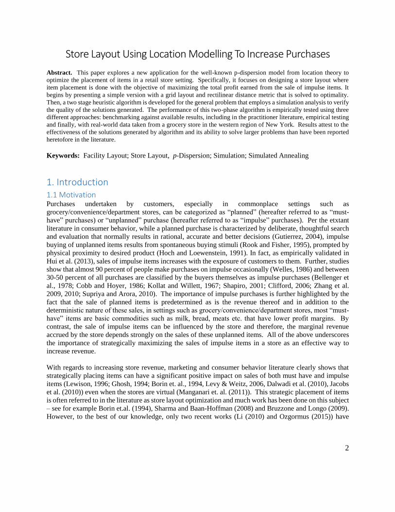
Figure 1: An Optimal Location of Must-Have Items in Grid Layout and Rectilinear

Metric

Let the shelves in the store be designated by 1,2,..n,.,N and assumed to be numbered from left to right as

shown in Figure 1 with a distance of W between adjacent shelves and assume that the store entrance is

immediately to the left of the first shelf, implying that is where all customer travel begins in the store.

Further, assume that each of these impenetrable shelves is of length L and negligible width, as shown in the

figure and that K=2N, implying that there are twice as many must-have items as shelves. All items are

located on the boundary of these N impenetrable rectangular shelves. Given that customer travel is

performed using rectilinear metric in the presence of barriers, it is easy to show that when a customer travels

2 The rectilinear distance between two points X1 = (x1, y1) and X2 = (x2, y2) is |x1-x2| + |y1-y2|.

SH

EL

F 1

SH

EL

F 2

SH

EL

F n

-1

SH

EL

F N

W

L

Must-

have

Items

6

between adjacent must-have items on the same shelf (say first two items from left located on Shelf 1 in

Figure 1), the shortest path is the travel along the boundary of the shelf itself – an example of this is

illustrated by dashed lines in the figure). It also readily follows that regardless of the path taken by any

customer, travelling between the N shelves to purchase the 2N must-have items necessitates any customer

to travel a minimum total inter-shelf distance of W((K-2)/2). Thus, any attempt to maximize a path taken

by any customer should focus solely on maximizing the distance travelled by him/her in picking adjacent

items located on either side of the same shelf (e.g., the distance between the first two items located on shelf

1 in Figure 1). It is easy to show that one configuration in which this is achieved is when both items are

located at the mid-point of each shelf, one on either side, as shown in Figure 1. The impulse items are then

placed on each shelf between the must-have items to expose them to the customers and the total distance

travelled by a customer is W ((K-2)/2) + KL. This is summarized as follows and illustrated in Figure 1.

Observation 1. Given rectangular impenetrable shelves with negligible widths, twice as many must-have

items as shelves and rectilinear distances, it may be assumed that an optimal placement of the must-have

items that maximizes the total distance travelled by a customer to W((K-2)/2) + KL by placing them at the

midpoint of each side of every shelf. Placing the impulse items between the must-have items then maximizes

their exposure to the customers.

3. Model Formulation For The General Problem This section will address the general version of the problem in this paper that seeks to optimally place must-

have items so that even when customers probabilistically select nearest-neighbor paths in purchasing them,

their travel inside the store is maximized. Placing the impulse items along this longest path then maximizes

their exposure to them and thus, the probability of making impulse purchases. It is helpful to note here that

each item is essentially what a retail store would consider a unique SKU (Stock Keeping Unit). We assume

that customers are heterogeneous in that a customer’s must-have item list depends on his/her individual

needs and thus, there exist different categories of customers with different sets of must-have items.

Specifically, we assume that there are K categories of customers, indexed by 𝑘 = 1, … , 𝐾 and let K =

1,…,K define the set of must-have items for customer category k. Furthermore, let k = 1,…k define the set

of impulse items for customer category k and li,k be the number of impulse items of type i purchased by

customer type k if they were to pass by this item type in their visit to the store. Finally, we let Ci denote

the marginal profit earned from a unit sale of item i, where this profit is assumed to be given as the

difference between unit sale price and the unit variable cost for this item. An inherent simplifying

assumption in this is that the store has information on all marginal operational costs related to a given item,

such as replenishment costs or holding costs and that these costs can be independently and accurately

ascribed to each item.

Let ∆ be the set of all possible layouts indexed by j and with elements denoted by Lj. That is Lj denotes a

specific layout or arrangement of items in the store. We let kj k denote the set of impulse items customer

type k passes while travelling in layout Lj and picking up his/her must-have items. Then the value of layout

Lj is given by:

 

,

1

 kj

K

i i k

k i

V j C

(1)

7

Therefore our problem can be formulated as:

(P) ( )

j

Max V j

L (2)

Due to the combinatorially large number of elements in , the problem (P) above is difficult to solve. We

therefore proceed by developing a two-stage heuristic which relies on the evaluation of V(j) for a specific

layout Lj . The data needed for evaluating this is as follows: the Ci be the marginal profit earned from a

unit sale of item i; K, the number of customer categories; the set of must-have items for a given customer

category and; set of impulse items for a given customer category. As mentioned before, we assume that (a)

the customer is inclined to buy impulse items if s/he passes by the items, (b) when customers travel between

must-have items, they select the next must-have item based on the distance from their current location – the

smaller the distance the greater the chance of selecting that particular must-have item, with ties broken

arbitrarily and (c) the distances are symmetric, i.e. the distance from location “A” to “B” is same as from

“B” to “A”.

In order to create the store layout and in-store travel pattern, we develop a graph representation of the store

layout, with nodes corresponding to the center of item storage department areas and arcs corresponding to

connections between the nodes. We do not assume that the customer’s path between must-have items is

deterministically known. Rather, we assume that given the current location of the customer, the likelihood

that s/he selects a particular must-have item to visit next is inversely proportional to its distance from her/his

current location and ties are broken arbitrarily. Given this probabilistic nature of the paths taken by the

different customers, computing the value of a store layout is a nontrivial problem. In order to address the

same, we developed a simulation code in VBA (Visual Basic) to evaluate the value of a layout. In that

simulation, for a given store layout, the customers are programmed as independent entities that move around

the store to pick up their must-have items and impulse items in accordance with the probabilistic choice

rule described above in selecting the sequence of items to purchase and the paths that they take to do the

same.

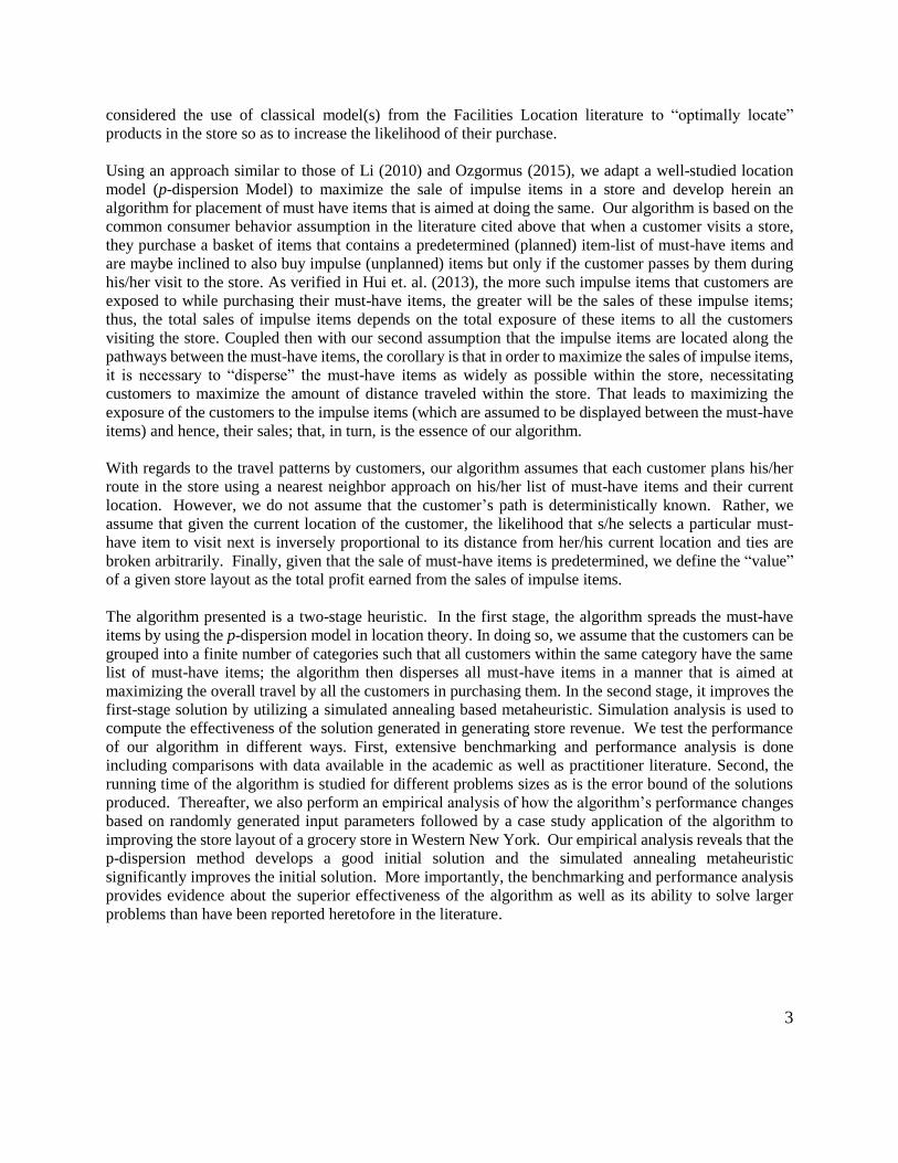
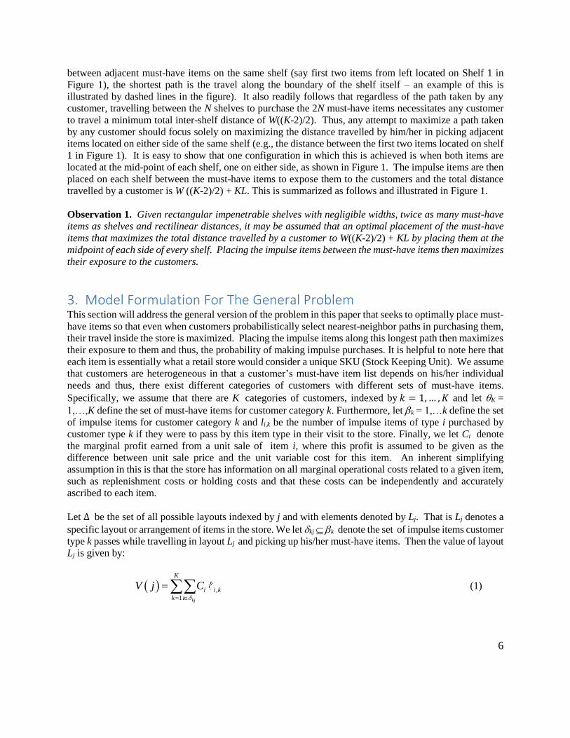
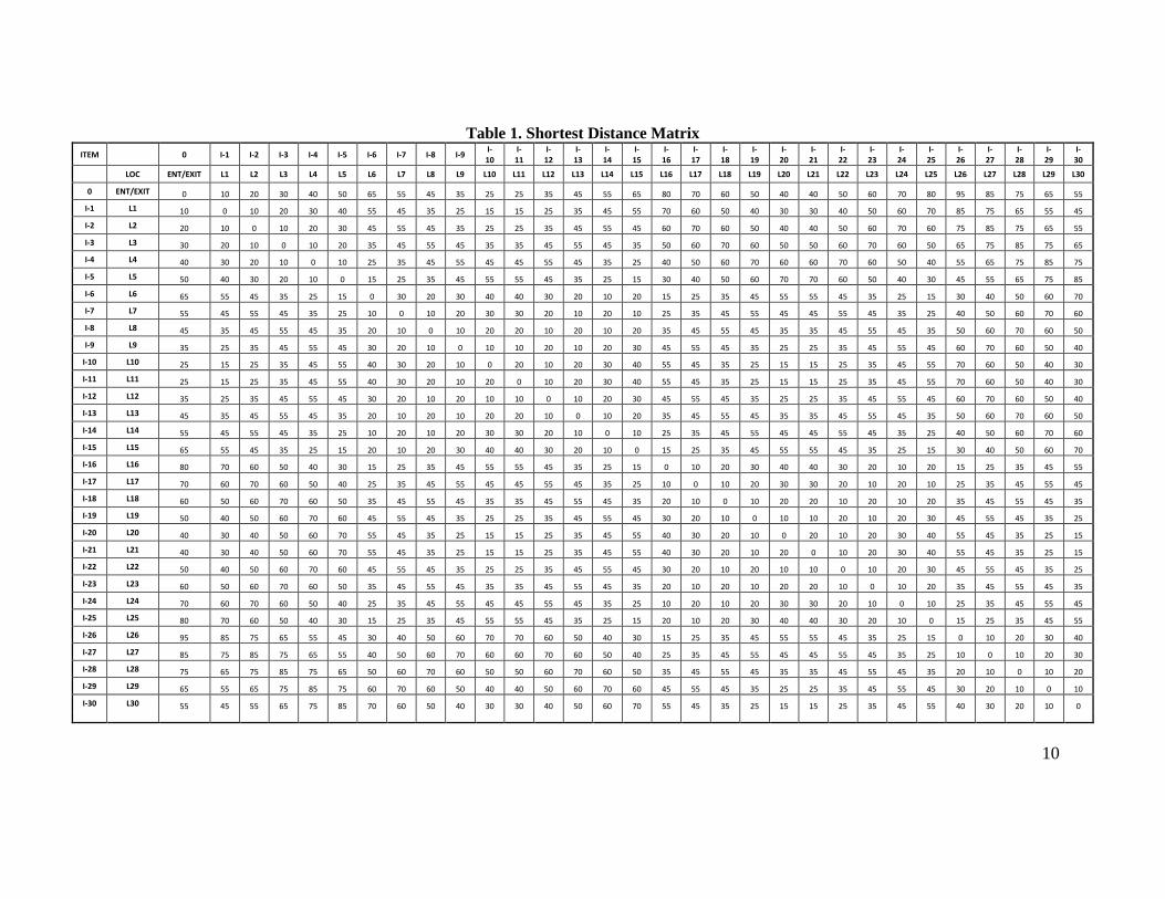
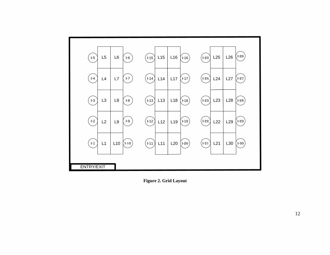
The above is best illustrated with an example and hence, consider the case of grocery store with the 30 item

store layout shown in Figure 2. The locations and shortest distances are given by the shortest distance matrix

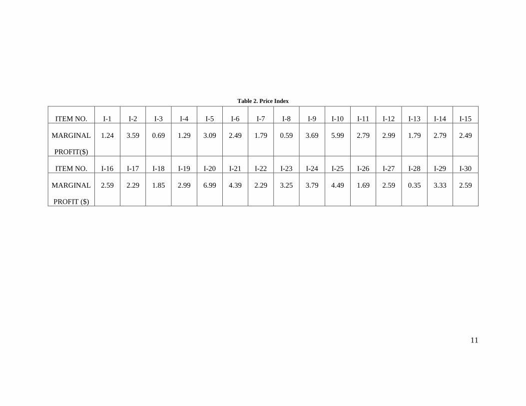
in Table 1. The cost of items is given in Table 2. Let there be a single customer category (i.e. K = 1) and

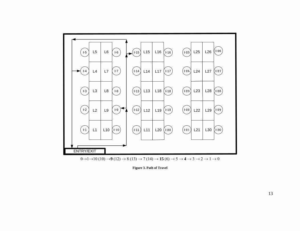
must-have and impulse items belonging to this category be 1 = {I-4, I-9, I-15} and 1 = {I-2, I-19, I-30}.

Based on the distance from the entrance that the first must-have item selected is: I-4 (36%), I-9 (42%), and

I-15 (22%). If the customer goes to I-9 first, based on the distance measurement from I-9 that the second

must-have item selected is: I-4 (35%), and I-15(65%). We present the path as Figure 3. The only impulse

item visited on this path is item I-2. The value of the layout using equation (1) is therefore given by:

 

,

1

      3.59  1  $ 3.59k

K

i i k

k i

V C

4 Solution Methodology: A Two-Phase Algorithm In this section, we present the details of our solution method to improve the impulse item revenues of the

grocery store. The method we employ is carried out in two phases. In the first phase we apply a heuristic

based on the p-dispersion model in location theory and then in the second phase we implement a simulated

8

annealing approach to improve upon the solution from the first phase. Moreover, we build a simulation

program to verify our solution method.

The p-dispersion problem is known to be an NP-hard problem whose objective is to disperse the entities as

far as possible in a given space. It is defined as selecting “p” out of “n” given points (1< p < n) in some

space, where the objective is to maximize the minimum distance between any two of the selected points

(Erkut, 1990). To maximally disperse the “p” points, maximally separated locations can be obtained by

applying the greedy deletion heuristic developed by Erkut et al. (1994). This heuristic starts with a solution

that contains all points and eliminates one point at each iteration, until “p” points are left. The point to be

eliminated is one of the two closest points in the current solution. Among those two points, the one that is

closest to the remaining points in the solution is eliminated. This is implemented in the first phase of our

solution methodology per the following algorithm.

1. Find the common must-have items across all K customer categories. Let there be p1 such items.

Use the p-dispersion heuristic with p = p1 to locate these items. Fix p1 must-have items at

maximally dispersed locations.

2. Find the common must-have items across K-1 customer categories. Let there be p2 such items. Use

the p-dispersion heuristic with p = p2 to locate these items. Fix p2 must-have items at maximally

dispersed locations.

3. Repeat until common must-have” items across K/2 customer categories are located using a p-

dispersion algorithm.

Once the “must- have” items are located, we derive the path taken by the customer to visit these must-have

items on his/her list and obtain the resulting value of the layout using the simulation described before.

In the second phase of our algorithm, simulated annealing starts with the layout obtained from the p-

dispersion based heuristic. The four basic ingredients required to solve simulated annealing are: a concise

description of the configuration of the system; a random generator of “moves” or rearrangements of

elements in a configuration; a quantitative objective function containing the trade-offs that have to be made

and an annealing schedule of temperatures, and; length of time for which the system is to be evolved

(Kirkpatrick et al., 1983). Given a particular layout and its associated value, as determined by the

simulation, the simulated annealing algorithm requires a systematic method for choosing another

neighboring solution in the next iteration. For our problem, a neighboring solution is generated by randomly

choosing two items from two different candidate sets and interchanging their locations. The two sets from

which items to be exchanged are selected from are: (i) must-have candidate set of m’ must-have items that

have not been moved from their original location and (ii) an Interchange candidate set comprising of (n-

m’) items other than must-have items that have not been moved from initial location.

At each iteration, a prospective solution is generated by defining a “pair-wise” exchange of must- have item

with a neighbor. If the prospective solution’s objective value is better than that of the best solution, then the

prospective solution is saved as the best solution and becomes the current solution. If the prospective

solution is not better than the best solution, then it may become the current solution with an acceptance

probability determined by temperature parameter (Reeves, 1993).

The probability of acceptance of an inferior solution, denoted by P(acceptance), at each iteration of the

simulated annealing algorithm is given by:

9

P (acceptance) = exp[V(j) – V(j0)]/t (3)

Where,

V(j) = objective value of the prospective layout j

V(j0) = objective value of the current layout j0 and

t = temperature.

The temperature is held fixed for each loop. At the end of each loop the temperature is dropped according

to the rule:

t = [(m’-mi)/m’] (4)

where;

= average value of items,

m’ = total number of items in must-have candidate set and,

mi = iteration number.

It is best to illustrate the working of the above 2-phase algorithm with a numerical example and hence, that

is what we do next. Consider the 30 item store layout shown in Figure 2. The locations and shortest

distances are given by the shortest distance matrix in Table 1. The unit marginal profits of the items is given

in Table 2. To test the p-dispersion based heuristic and simulated annealing approach we developed a

simulation program and ran it for the case of K=3 (i.e. three customer categories). The set of items for the

three customer categories were as follows:

Category I: Must-have items k = {I-2, I-11, I-12, I-13, I-23, I-25} and

Impulse items k = {I-7, I-28}

Category II: Must-have items k = {I-2, I-11, I-12, I-20, I-22, I-30} and

Impulse items k = {I-15, I-16}

Category III: Must-have items k = {I-2, I-3, I-11, I-12, I-20, I-22} and

Impulse items k = {I-24, I-29}

The value of the original layout based on the average obtained from ten runs of the simulation program was

found to be V = 8.23.

10

Table 1. Shortest Distance Matrix

ITEM 0 I-1 I-2 I-3 I-4 I-5 I-6 I-7 I-8 I-9 I-10

I-11

I-12

I-13

I-14

I-15

I-16

I-17

I-18

I-19

I-20

I-21

I-22

I-23

I-24

I-25

I-26

I-27

I-28

I-29

I-30

LOC ENT/EXIT L1 L2 L3 L4 L5 L6 L7 L8 L9 L10 L11 L12 L13 L14 L15 L16 L17 L18 L19 L20 L21 L22 L23 L24 L25 L26 L27 L28 L29 L30

0 ENT/EXIT 0 10 20 30 40 50 65 55 45 35 25 25 35 45 55 65 80 70 60 50 40 40 50 60 70 80 95 85 75 65 55

I-1 L1 10 0 10 20 30 40 55 45 35 25 15 15 25 35 45 55 70 60 50 40 30 30 40 50 60 70 85 75 65 55 45

I-2 L2 20 10 0 10 20 30 45 55 45 35 25 25 35 45 55 45 60 70 60 50 40 40 50 60 70 60 75 85 75 65 55

I-3 L3 30 20 10 0 10 20 35 45 55 45 35 35 45 55 45 35 50 60 70 60 50 50 60 70 60 50 65 75 85 75 65

I-4 L4 40 30 20 10 0 10 25 35 45 55 45 45 55 45 35 25 40 50 60 70 60 60 70 60 50 40 55 65 75 85 75

I-5 L5 50 40 30 20 10 0 15 25 35 45 55 55 45 35 25 15 30 40 50 60 70 70 60 50 40 30 45 55 65 75 85

I-6 L6 65 55 45 35 25 15 0 30 20 30 40 40 30 20 10 20 15 25 35 45 55 55 45 35 25 15 30 40 50 60 70

I-7 L7 55 45 55 45 35 25 10 0 10 20 30 30 20 10 20 10 25 35 45 55 45 45 55 45 35 25 40 50 60 70 60

I-8 L8 45 35 45 55 45 35 20 10 0 10 20 20 10 20 10 20 35 45 55 45 35 35 45 55 45 35 50 60 70 60 50

I-9 L9 35 25 35 45 55 45 30 20 10 0 10 10 20 10 20 30 45 55 45 35 25 25 35 45 55 45 60 70 60 50 40

I-10 L10 25 15 25 35 45 55 40 30 20 10 0 20 10 20 30 40 55 45 35 25 15 15 25 35 45 55 70 60 50 40 30

I-11 L11 25 15 25 35 45 55 40 30 20 10 20 0 10 20 30 40 55 45 35 25 15 15 25 35 45 55 70 60 50 40 30

I-12 L12 35 25 35 45 55 45 30 20 10 20 10 10 0 10 20 30 45 55 45 35 25 25 35 45 55 45 60 70 60 50 40

I-13 L13 45 35 45 55 45 35 20 10 20 10 20 20 10 0 10 20 35 45 55 45 35 35 45 55 45 35 50 60 70 60 50

I-14 L14 55 45 55 45 35 25 10 20 10 20 30 30 20 10 0 10 25 35 45 55 45 45 55 45 35 25 40 50 60 70 60

I-15 L15 65 55 45 35 25 15 20 10 20 30 40 40 30 20 10 0 15 25 35 45 55 55 45 35 25 15 30 40 50 60 70

I-16 L16 80 70 60 50 40 30 15 25 35 45 55 55 45 35 25 15 0 10 20 30 40 40 30 20 10 20 15 25 35 45 55

I-17 L17 70 60 70 60 50 40 25 35 45 55 45 45 55 45 35 25 10 0 10 20 30 30 20 10 20 10 25 35 45 55 45

I-18 L18 60 50 60 70 60 50 35 45 55 45 35 35 45 55 45 35 20 10 0 10 20 20 10 20 10 20 35 45 55 45 35

I-19 L19 50 40 50 60 70 60 45 55 45 35 25 25 35 45 55 45 30 20 10 0 10 10 20 10 20 30 45 55 45 35 25

I-20 L20 40 30 40 50 60 70 55 45 35 25 15 15 25 35 45 55 40 30 20 10 0 20 10 20 30 40 55 45 35 25 15

I-21 L21 40 30 40 50 60 70 55 45 35 25 15 15 25 35 45 55 40 30 20 10 20 0 10 20 30 40 55 45 35 25 15

I-22 L22 50 40 50 60 70 60 45 55 45 35 25 25 35 45 55 45 30 20 10 20 10 10 0 10 20 30 45 55 45 35 25

I-23 L23 60 50 60 70 60 50 35 45 55 45 35 35 45 55 45 35 20 10 20 10 20 20 10 0 10 20 35 45 55 45 35

I-24 L24 70 60 70 60 50 40 25 35 45 55 45 45 55 45 35 25 10 20 10 20 30 30 20 10 0 10 25 35 45 55 45

I-25 L25 80 70 60 50 40 30 15 25 35 45 55 55 45 35 25 15 20 10 20 30 40 40 30 20 10 0 15 25 35 45 55

I-26 L26 95 85 75 65 55 45 30 40 50 60 70 70 60 50 40 30 15 25 35 45 55 55 45 35 25 15 0 10 20 30 40

I-27 L27 85 75 85 75 65 55 40 50 60 70 60 60 70 60 50 40 25 35 45 55 45 45 55 45 35 25 10 0 10 20 30

I-28 L28 75 65 75 85 75 65 50 60 70 60 50 50 60 70 60 50 35 45 55 45 35 35 45 55 45 35 20 10 0 10 20

I-29 L29 65 55 65 75 85 75 60 70 60 50 40 40 50 60 70 60 45 55 45 35 25 25 35 45 55 45 30 20 10 0 10

I-30 L30 55 45 55 65 75 85 70 60 50 40 30 30 40 50 60 70 55 45 35 25 15 15 25 35 45 55 40 30 20 10 0

11

Table 2. Price Index

ITEM NO. I-1 I-2 I-3 I-4 I-5 I-6 I-7 I-8 I-9 I-10 I-11 I-12 I-13 I-14 I-15

MARGINAL

PROFIT($)

1.24 3.59 0.69 1.29 3.09 2.49 1.79 0.59 3.69 5.99 2.79 2.99 1.79 2.79 2.49

ITEM NO. I-16 I-17 I-18 I-19 I-20 I-21 I-22 I-23 I-24 I-25 I-26 I-27 I-28 I-29 I-30

MARGINAL

PROFIT ($)

2.59 2.29 1.85 2.99 6.99 4.39 2.29 3.25 3.79 4.49 1.69 2.59 0.35 3.33 2.59

12

L5

L4

L3

L2

L1

L6

L7

L8

L9

L10

L15

L14

L13

L12

L11

L16

L17

L18

L19

L20

ENTRY/EXIT

L25

L24

L23

L22

L21

L26

L27

L28

L29

L30I-11

I-12

I-13

I-14

I-15

I-20

I-19

I-18

I-17

I-16

I-21

I-22

I-23

I-24

I-25

I-30

I-29

I-28

I-27

I-26

I-1

I-2

I-3

I-4

I-5

I-10

I-9

I-8

I-7

I-6

Figure 2. Grid Layout

13

L5

L4

L3

L2

L1

L6

L7

L8

L9

L10

L15

L14

L13

L12

L11

L16

L17

L18

L19

L20

ENTRY/EXIT

L25

L24

L23

L22

L21

L26

L27

L28

L29

L30I-11

I-12

I-13

I-14

I-15

I-20

I-19

I-18

I-17

I-16

I-21

I-22

I-23

I-24

I-25

I-30

I-29

I-28

I-27

I-26

I-1

I-2

I-3

I-4

I-5

I-10

I-9

I-8

I-7

I-6

0→1→10 (10) →9 (12) → 8 (13) → 7 (14) → 15 (6) → 5 → 4 → 3 → 2 → 1 → 0

Figure 3. Path of Travel

14

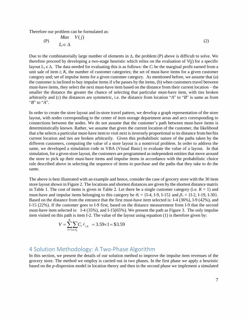
Let us now improve this current layout above by using the 1st phase of our algorithm that uses the p-

dispersion heuristic. We start by applying this heuristic to all K=3 categories of customers and derive the

value p (p common points) based on the example. Three must-have items I-2, I-11, and I-12 are common

to all customer categories; hence the initial value of p is equal to p1=3. The three maximally dispersed

locations obtained from the greedy deletion heuristic are L8, L18 and L28. We then exchange the locations

of I-2, I-11, and I-12 with I-8, I-18, and I-28 respectively and fix these must-have items at these locations.

We again apply the p-dispersion based heuristic to find the common must-have items in K-1 customer

categories. Two items I-20 and I-22 are common to Category II and Category III; hence the second value

of p is p2 = 2. We then obtain L5 and L30 as the two maximally dispersed locations from the greedy deletion

heuristic. Items I-20 and I-22 are exchanged with I-5 and I-30 respectively and the must-have items are

fixed at these locations. The value of this new layout (again obtained by taking the average of ten runs of

the simulation program) was found to be V =13.25.

Next, we apply the second phase of the algorithm and further improve the layout using simulated annealing,

which leads us to exchange locations I-4 and I-25 with I-23 and I-26, respectively. The value of this revised

layout as obtained by taking the average of ten runs of the simulation program was found to be V = 14.04.

Therefore in this example it can be seen that the p-dispersion phase yields a significant increase in value of

the layout, whereas the simulated annealing phase yields a marginal further improvement.

5 Benchmarking and Performance Analysis This section focuses on analyzing the performance of our all using two different approaches. The first

approach is to perform an extensive empirical study to determine the effectiveness of the algorithm wherein

we test the behavior of the algorithm when the factors that affect the computational complexity of the input

parameters are varied. The second part of the analysis benchmarks the results from the algorithm against

available results in the academic as well as practitioner literature. Thereafter, we determine the growth in

the time taken by the algorithm to solve increasingly larger problems and empirically estimate the error

bounds of the solutions produced by this algorithm.

5.1 Empirical Analysis Paired T-test

Here, we wanted to empirically test whether or not our algorithm improved the value of a store’s layout and

if so, what the average improvement would be. To that end, we selected 16 different grid patterns similar

to the one shown in Figure 2 with the total number of items (must-have and impulse) ranging from 30-45.

For each such test case, we randomly picked must-have items and impulse items and assigned them

randomly to the placement spots available (similar to Figure 2, the number of placement spots in the grid

pattern was equal to the number of items to be placed in each test case) to determine the original layout.

Then, we ran each phase of our two phase algorithm. For every layout, the initial one as well as the ones

produced at the end of each phase of our algorithm, the VBA simulation code was used 10 times and the

average of these 10 simulations was denoted as the value of that layout. We then tested the results from

these 16 experiments for impulse value for the original layout and the same for the improved layouts

produced by the p-dispersion heuristic (1st phase of our algorithm) and simulated annealing (2nd phase of

our algorithm). The results of the paired t-test for p-dispersed impulse value minus initial impulse value are

displayed in Table 3.

15

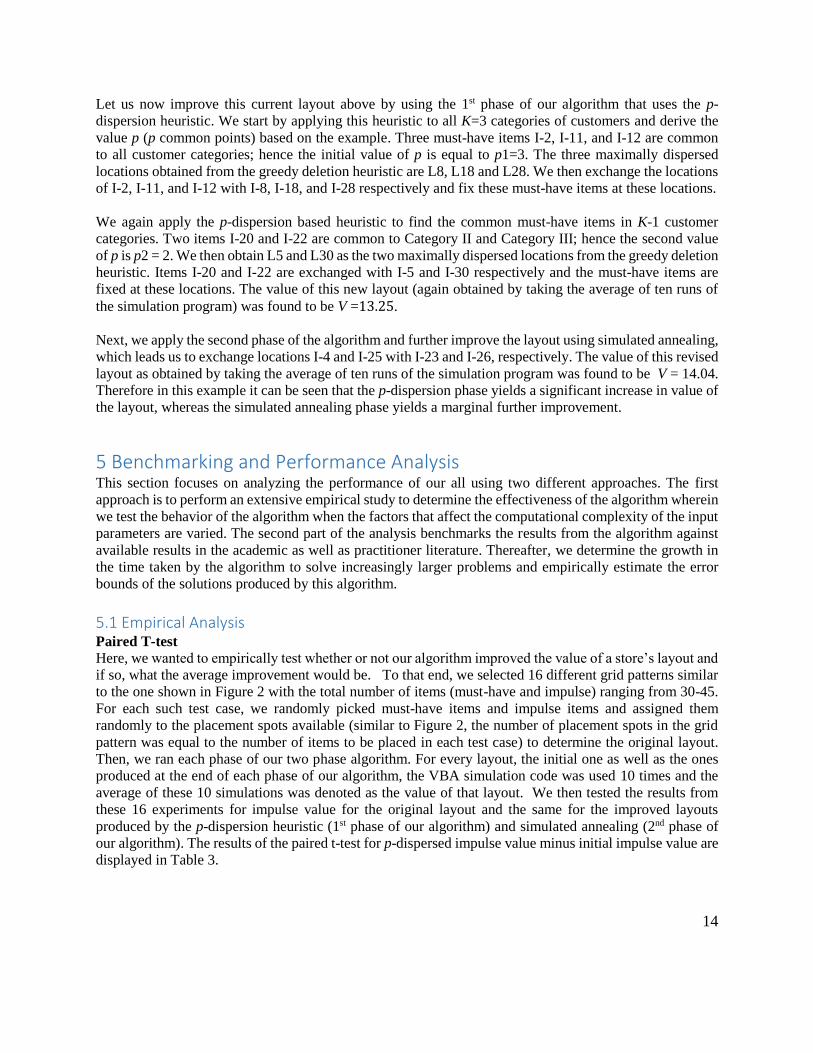
Table 3. Paired T-Test p-dispersed impulse value minus Original impulse value

N Mean StDev SE

Mean

p-dispersed impulse value 16 15.18 3.17 0.79

Original impulse value 16 13.66 3.46 0.87

Difference 16 1.53 0.29 0.08

95% CI for mean difference: (-2.164, -0.873)

T-Test of mean difference = 0 (vs not = 0): T-Value = -5.01 P-Value = 0.000

From Table 3, we see that the P-Value of the test is 0. This suggests that there is a significant difference in

the impulse values of the p-dispersed layout and the original layout. Specifically, the p -dispersed impulse

value (mean = 14.47) is higher than the original impulse value (mean = 12.13). Therefore, there is a

significant increase in impulse value through implementation of the p-dispersion based heuristic.

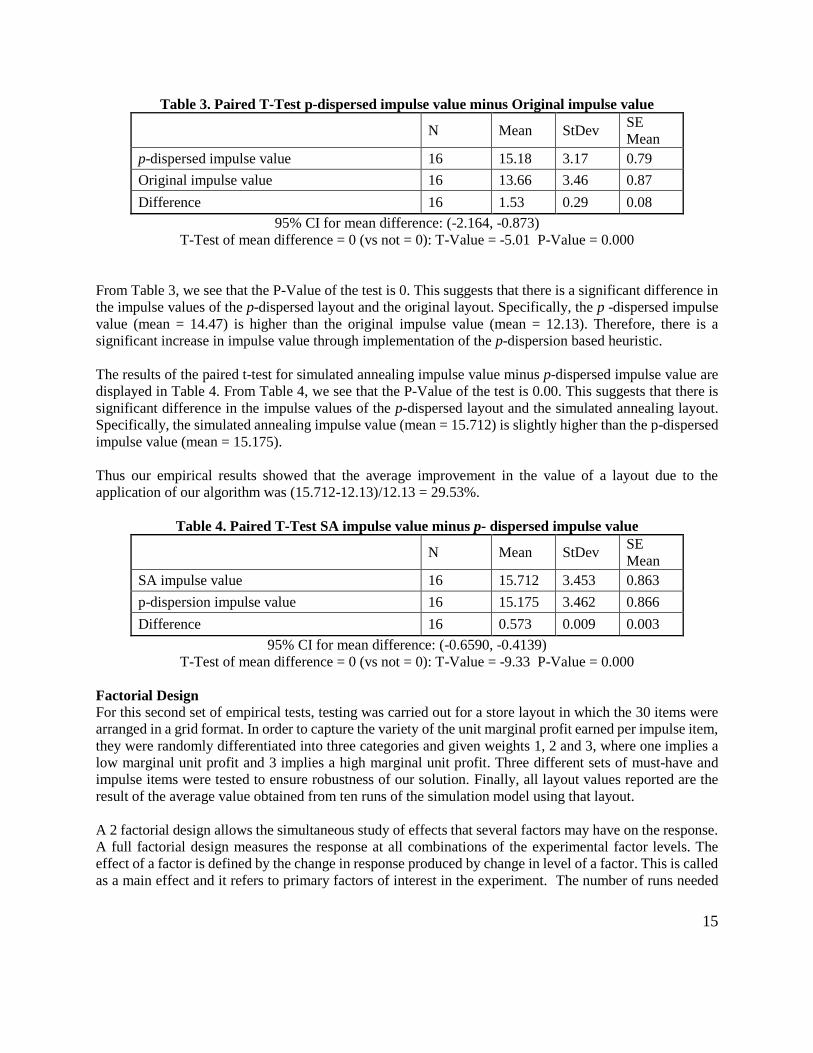
The results of the paired t-test for simulated annealing impulse value minus p-dispersed impulse value are

displayed in Table 4. From Table 4, we see that the P-Value of the test is 0.00. This suggests that there is

significant difference in the impulse values of the p-dispersed layout and the simulated annealing layout.

Specifically, the simulated annealing impulse value (mean = 15.712) is slightly higher than the p-dispersed

impulse value (mean = 15.175).

Thus our empirical results showed that the average improvement in the value of a layout due to the

application of our algorithm was (15.712-12.13)/12.13 = 29.53%.

Table 4. Paired T-Test SA impulse value minus p- dispersed impulse value

N Mean StDev SE

Mean

SA impulse value 16 15.712 3.453 0.863

p-dispersion impulse value 16 15.175 3.462 0.866

Difference 16 0.573 0.009 0.003

95% CI for mean difference: (-0.6590, -0.4139)

T-Test of mean difference = 0 (vs not = 0): T-Value = -9.33 P-Value = 0.000

Factorial Design

For this second set of empirical tests, testing was carried out for a store layout in which the 30 items were

arranged in a grid format. In order to capture the variety of the unit marginal profit earned per impulse item,

they were randomly differentiated into three categories and given weights 1, 2 and 3, where one implies a

low marginal unit profit and 3 implies a high marginal unit profit. Three different sets of must-have and

impulse items were tested to ensure robustness of our solution. Finally, all layout values reported are the

result of the average value obtained from ten runs of the simulation model using that layout.

A 2 factorial design allows the simultaneous study of effects that several factors may have on the response.

A full factorial design measures the response at all combinations of the experimental factor levels. The

effect of a factor is defined by the change in response produced by change in level of a factor. This is called

as a main effect and it refers to primary factors of interest in the experiment. The number of runs needed

16

to exhaust all combinations for our 2 factorial design is 8. We took 3 replications at each run for a total of

24 data points. The algorithms were tested for all possible combinations and output parameters recorded.

Graphs were plotted to determine the significance of each factor.

Since the essential objective of the algorithm is to maximally disperse the must-have items to increase the

number of impulse buys in the store, the output parameter of interest is the impulse value (aggregate

marginal profit) of the layout. Considering the influences of those factors significant to the improvement

of value, we also need to analyze the nuances between the original layout and the one that applies our

algorithm. To that end, we divided the factors into two groups: Customer segmentation factors (number of

customer categories) and Algorithmic factors (Number of common must-have items and total number of

must-have items). Additionally, these factors have to be varied to determine the response at all

combinations of the experimental factor levels since the effect of a factor is defined by the change in

response produced by change in level of a factor. In this case, we varied the factors at two levels: LOW and

HIGH. The resulting values of different factors levels are found in Table 5.

Table 5. Factor Levels

Factor Type Factor LOW HIGH

Customer Factor No. of customer categories 3 5

Algorithmic Factor Common must-have items 2 4

Algorithmic Factor Number of must-have items 4 6

We performed ANOVA of two different groups of customers to understand the significance of different

factors. The ANOVA Table for main effects is shown in Table 6 and Table 7.

Table 6. ANOVA Table (Impulse value group 1)

Source DF Seq SS Adj SS Adj MS F p

No. of Common must have

items

1 0.344 0.344 0.344 0.45 0.511

No. of must have item 1 11.363 11.363 11.363 14.79 0.001

No. of Customer categories 1 371.633 371.633 371.633 483.83 0.000

Table 7. ANOVA Table (Impulse value group 2)

Source DF Seq SS Adj SS Adj MS F p

No. of Common must have

items

1 1.118 1.118 1.118 1.330 0.263

No. of must have item 1 11.833 11.833 11.833 14.040 0.001

No. of Customer categories 1 363.712 363.712 363.712 431.440 0.000

It can be seen from the analysis in Table 6 and Table 7, that the main effects ‘No. of Customer Categories’

and ‘No. of must-have items’ are significant. The R2 value of 95.57 % and 95.07% (refer to Appendix B

17

and Appendix C) shows that the main effects explain the variance in impulse value extremely well. The

regression equations of two different groups we derive from our analysis are:

Impulse Value = 17.14 -0.1197 (No. of Common must have item) + 0.6881 (No. of must-

have items) + 3.94 (No. of Customer Categories)

and

Impulse Value = 17.17 - 0.2159 (No. of Common must have item) + 0.7 (No. of must-have

items) + 3.89 (No. of Customer Categories)

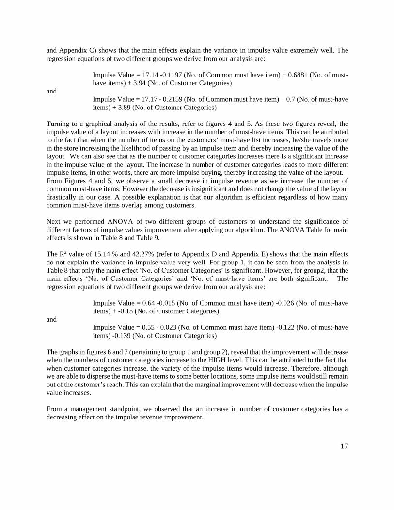
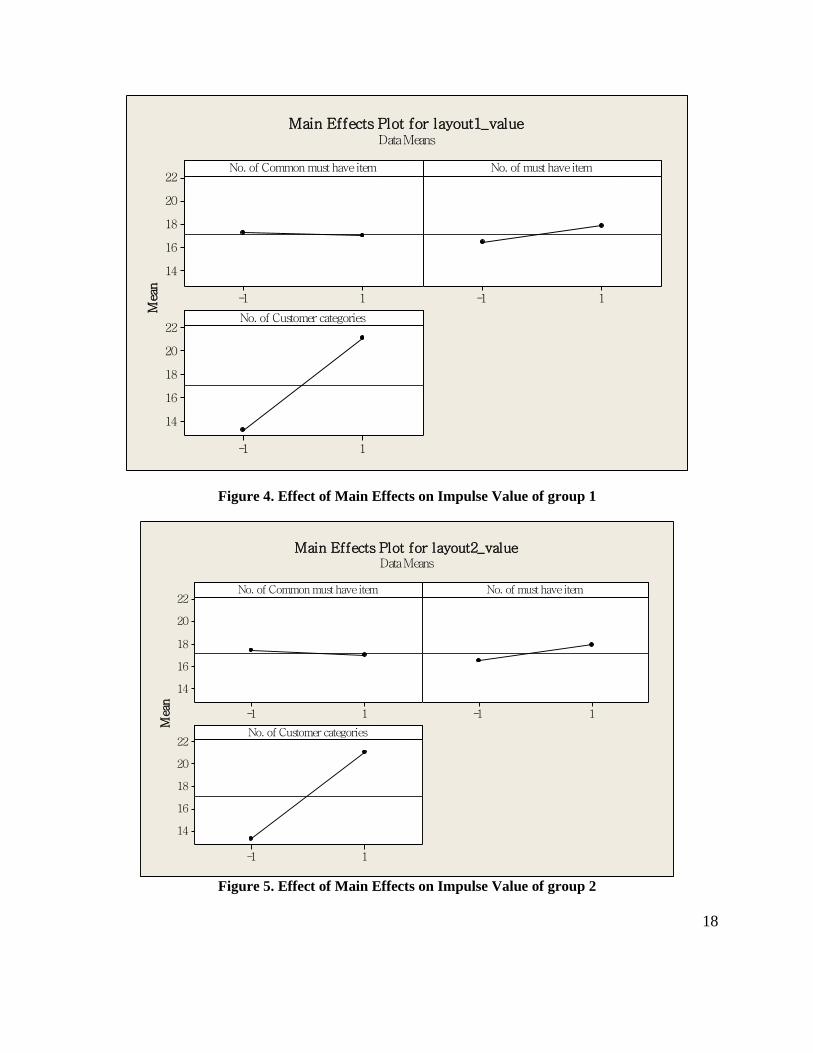
Turning to a graphical analysis of the results, refer to figures 4 and 5. As these two figures reveal, the

impulse value of a layout increases with increase in the number of must-have items. This can be attributed

to the fact that when the number of items on the customers’ must-have list increases, he/she travels more

in the store increasing the likelihood of passing by an impulse item and thereby increasing the value of the

layout. We can also see that as the number of customer categories increases there is a significant increase

in the impulse value of the layout. The increase in number of customer categories leads to more different

impulse items, in other words, there are more impulse buying, thereby increasing the value of the layout.

From Figures 4 and 5, we observe a small decrease in impulse revenue as we increase the number of

common must-have items. However the decrease is insignificant and does not change the value of the layout

drastically in our case. A possible explanation is that our algorithm is efficient regardless of how many

common must-have items overlap among customers.

Next we performed ANOVA of two different groups of customers to understand the significance of

different factors of impulse values improvement after applying our algorithm. The ANOVA Table for main

effects is shown in Table 8 and Table 9.

The R2 value of 15.14 % and 42.27% (refer to Appendix D and Appendix E) shows that the main effects

do not explain the variance in impulse value very well. For group 1, it can be seen from the analysis in

Table 8 that only the main effect ‘No. of Customer Categories’ is significant. However, for group2, that the

main effects ‘No. of Customer Categories’ and ‘No. of must-have items’ are both significant. The

regression equations of two different groups we derive from our analysis are:

Impulse Value = 0.64 -0.015 (No. of Common must have item) -0.026 (No. of must-have

items) + -0.15 (No. of Customer Categories)

and

Impulse Value = 0.55 - 0.023 (No. of Common must have item) -0.122 (No. of must-have

items) -0.139 (No. of Customer Categories)

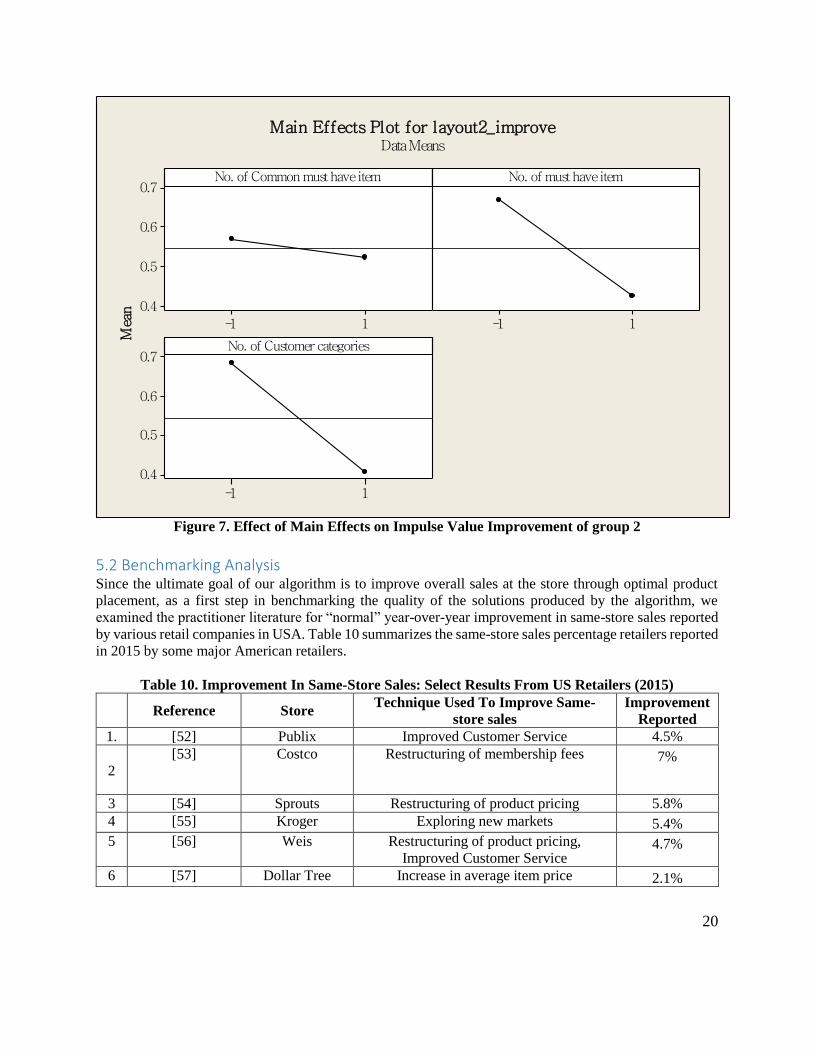
The graphs in figures 6 and 7 (pertaining to group 1 and group 2), reveal that the improvement will decrease

when the numbers of customer categories increase to the HIGH level. This can be attributed to the fact that

when customer categories increase, the variety of the impulse items would increase. Therefore, although

we are able to disperse the must-have items to some better locations, some impulse items would still remain

out of the customer’s reach. This can explain that the marginal improvement will decrease when the impulse

value increases.

From a management standpoint, we observed that an increase in number of customer categories has a

decreasing effect on the impulse revenue improvement.

18

1-1

22

20

18

16

14

1-1

1-1

22

20

18

16

14

No. of Common must have item

Mea

nNo. of must have item

No. of Customer categories

Main Effects Plot for layout1_valueData Means

Figure 4. Effect of Main Effects on Impulse Value of group 1

1-1

22

20

18

16

14

1-1

1-1

22

20

18

16

14

No. of Common must have item

Mea

n

No. of must have item

No. of Customer categories

Main Effects Plot for layout2_valueData Means

Figure 5. Effect of Main Effects on Impulse Value of group 2

19

Table 8. ANOVA Table (Impulse Value Improvement of group 1)

Source DF Seq SS Adj SS Adj MS F p

No. of Common must have

items

1 0.00526 0.00526 0.005256

0.07

0.800

No. of must have item 1 0.01592 0.01592 0.015918 0.200 0.66

No. of Customer

categories

1 0.54531 0.54531 0.545313 6.840 0.017

Table 9. ANOVA Table (Impulse Value Improvement group 2)

Source DF Seq SS Adj SS Adj MS F p

No. of Common must have

items

1 0.01271 0.01271 0.01271 0.30 0.589

No. of must have item 1 0.35956 0.35956 0.35956 8.54 0.008

No. of Customer

categories

1 0.46273 0.46273 0.46273 11 0.003

1-1

0.8

0.7

0.6

0.5

1-1

1-1

0.8

0.7

0.6

0.5

No. of Common must have item

Mea

n

No. of must have item

No. of Customer categories

Main Effects Plot for layout1_improveData Means

Figure 6. Effect of Main Effects on Impulse Value Improvement of group 1

20

1-1

0.7

0.6

0.5

0.4

1-1

1-1

0.7

0.6

0.5

0.4

No. of Common must have item

Mea

n

No. of must have item

No. of Customer categories

Main Effects Plot for layout2_improveData Means

Figure 7. Effect of Main Effects on Impulse Value Improvement of group 2

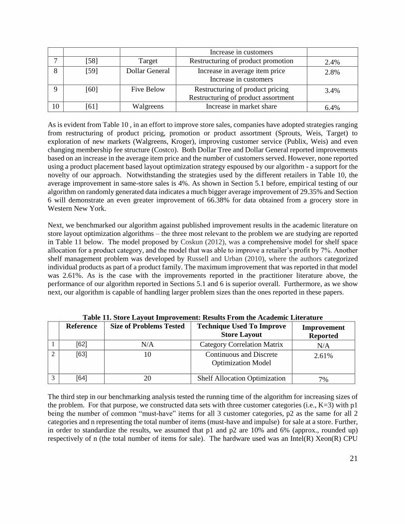
5.2 Benchmarking Analysis Since the ultimate goal of our algorithm is to improve overall sales at the store through optimal product

placement, as a first step in benchmarking the quality of the solutions produced by the algorithm, we

examined the practitioner literature for “normal” year-over-year improvement in same-store sales reported

by various retail companies in USA. Table 10 summarizes the same-store sales percentage retailers reported

in 2015 by some major American retailers.

Table 10. Improvement In Same-Store Sales: Select Results From US Retailers (2015)

Reference Store

Technique Used To Improve Same-

store sales

Improvement

Reported

1. [52] Publix Improved Customer Service 4.5%

2

[53] Costco Restructuring of membership fees 7%

3 [54] Sprouts Restructuring of product pricing 5.8%

4 [55] Kroger Exploring new markets 5.4%

5 [56] Weis Restructuring of product pricing,

Improved Customer Service 4.7%

6 [57] Dollar Tree Increase in average item price 2.1%

21

Increase in customers

7 [58] Target Restructuring of product promotion 2.4%

8 [59] Dollar General Increase in average item price

Increase in customers 2.8%

9 [60] Five Below Restructuring of product pricing

Restructuring of product assortment 3.4%

10 [61] Walgreens Increase in market share 6.4%

As is evident from Table 10 , in an effort to improve store sales, companies have adopted strategies ranging

from restructuring of product pricing, promotion or product assortment (Sprouts, Weis, Target) to

exploration of new markets (Walgreens, Kroger), improving customer service (Publix, Weis) and even

changing membership fee structure (Costco). Both Dollar Tree and Dollar General reported improvements

based on an increase in the average item price and the number of customers served. However, none reported

using a product placement based layout optimization strategy espoused by our algorithm - a support for the

novelty of our approach. Notwithstanding the strategies used by the different retailers in Table 10, the

average improvement in same-store sales is 4%. As shown in Section 5.1 before, empirical testing of our

algorithm on randomly generated data indicates a much bigger average improvement of 29.35% and Section

6 will demonstrate an even greater improvement of 66.38% for data obtained from a grocery store in

Western New York.

Next, we benchmarked our algorithm against published improvement results in the academic literature on

store layout optimization algorithms – the three most relevant to the problem we are studying are reported

in Table 11 below. The model proposed by Coskun (2012), was a comprehensive model for shelf space

allocation for a product category, and the model that was able to improve a retailer’s profit by 7%. Another

shelf management problem was developed by Russell and Urban (2010), where the authors categorized

individual products as part of a product family. The maximum improvement that was reported in that model

was 2.61%. As is the case with the improvements reported in the practitioner literature above, the

performance of our algorithm reported in Sections 5.1 and 6 is superior overall. Furthermore, as we show

next, our algorithm is capable of handling larger problem sizes than the ones reported in these papers.

Table 11. Store Layout Improvement: Results From the Academic Literature

Reference Size of Problems Tested Technique Used To Improve

Store Layout Improvement

Reported 1 [62] N/A Category Correlation Matrix N/A 2 [63]

10 Continuous and Discrete

Optimization Model 2.61%

3 [64] 20 Shelf Allocation Optimization 7%

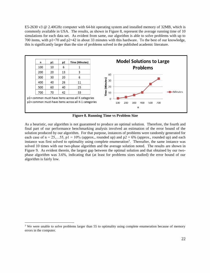
The third step in our benchmarking analysis tested the running time of the algorithm for increasing sizes of

the problem. For that purpose, we constructed data sets with three customer categories (i.e., K=3) with p1

being the number of common “must-have” items for all 3 customer categories, p2 as the same for all 2

categories and n representing the total number of items (must-have and impulse) for sale at a store. Further,

in order to standardize the results, we assumed that p1 and p2 are 10% and 6% (approx., rounded up)

respectively of n (the total number of items for sale). The hardware used was an Intel(R) Xeon(R) CPU

22

E5-2630 v3 @ 2.40GHz computer with 64-bit operating system and installed memory of 32MB, which is

commonly available in USA. The results, as shown in Figure 8, represent the average running time of 10

simulations for each data set. As evident from same, our algorithm is able to solve problems with up to

700 items, with p1=70 and p2=42 in about 33 minutes with this hardware. To the best of our knowledge,

this is significantly larger than the size of problems solved in the published academic literature.

Figure 8. Running Time vs Problem Size

As a heuristic, our algorithm is not guaranteed to produce an optimal solution. Therefore, the fourth and

final part of our performance benchmarking analysis involved an estimation of the error bound of the

solution produced by our algorithm. For that purpose, instances of problems were randomly generated for

each case of n = 25,…55, p1 = 10% (approx., rounded up) and p2 = 6% (approx., rounded up) and each

instance was first solved to optimality using complete enumeration3. Thereafter, the same instance was

solved 10 times with our two-phase algorithm and the average solution noted. The results are shown in

Figure 9. As evident therein, the largest gap between the optimal solution and that obtained by our two-

phase algorithm was 3.6%, indicating that (at least for problems sizes studied) the error bound of our

algorithm is fairly low.

3 We were unable to solve problems larger than 55 to optimality using complete enumeration because of memory

errors in the computer.

23

Figure 9. Error Bound

In concluding this section on analyzing the performance of our algorithm, the benchmarking done and the

subsequent empirical analysis based on randomly generated data allow us to make the following

observations.

(1) The statistical results suggests that the two-phase algorithm proposed with p-dispersion

based heuristic in the first phase followed by simulated annealing metaheuristic in the

second, are effective in increasing the impulse value of the layout. Per the experiments,

the average improvement in the value of a layout reported in our empirical study is 29.53%.

(2) The p-dispersion based heuristic gives a good starting solution with a significantly

improved layout in terms of impulse revenue and thereafter, the simulated annealing

metaheuristic improves the initial solution provided by the p-dispersion based heuristic

method.

(3) The benchmarking analysis performed shows that our two-phase algorithm produces

improvements that are superior to those reported in the academic as well as practitioner

literature. Further, the algorithm is capable of solving larger problems that those reported

heretofore in the academic literature.

(4) The error bound of the solutions produced by our two-phase algorithm is small and

below 5% for all the cases we tested.

6. Case Study In an effort to investigate the efficacy of our proposed algorithm in a real-world setting, we tested its

practical for the layout of a grocery store in Western New York, whose identity is withheld upon the request

of store management. The targeted grocery store stocks fresh vegetables every Thursday. Therefore, buying

fresh vegetables is the main reason for almost every customer who visits the store on Thursdays. However,

store management felt that the display of vegetables was not spatially dispersed enough to make customers

travel around the store, leading to poor impulse buying. That, in turn, why this store was selected for the

case study. Data collection has been described in Appendix A. As, mentioned therein, 50 samples were

24

collected, and based on the list of identified must-have items, we classified the customers into three

categories. For each of these three categories, we also identified the list of impulse items by analyzing the

survey data.

Based on these categories, we ran the simulation program for ten runs and took the average value. For the

original layout, the result was V = 10.65. For the layout obtained after p-dispersion phase of our algorithm

the result improved to V = 16.38 and finally, after the completion of the second phase involving the

simulated annealing metaheuristic, the impulse value of the layout reached V = 17.72. Thus, the value of

the new layout had a significant improvement compared to the original layout with an overall improvement

of 66.38%. In other words, the results from our case study based on an actual grocery store environment

matched those from our computational analysis in that significant improvements were achieved by applying

our two-phase algorithm to optimize the layout by dispersing the must-have items to maximize the sales of

the impulse items.

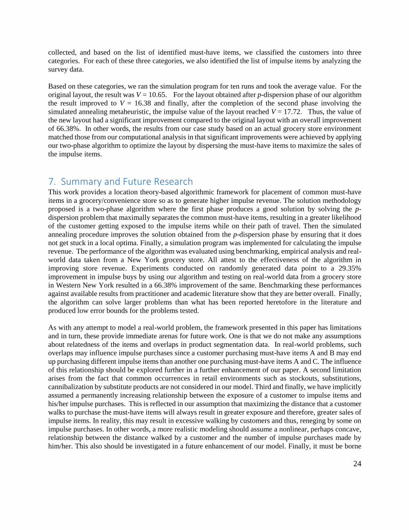
7. Summary and Future Research This work provides a location theory-based algorithmic framework for placement of common must-have

items in a grocery/convenience store so as to generate higher impulse revenue. The solution methodology

proposed is a two-phase algorithm where the first phase produces a good solution by solving the p-

dispersion problem that maximally separates the common must-have items, resulting in a greater likelihood

of the customer getting exposed to the impulse items while on their path of travel. Then the simulated

annealing procedure improves the solution obtained from the p-dispersion phase by ensuring that it does

not get stuck in a local optima. Finally, a simulation program was implemented for calculating the impulse

revenue. The performance of the algorithm was evaluated using benchmarking, empirical analysis and real-

world data taken from a New York grocery store. All attest to the effectiveness of the algorithm in

improving store revenue. Experiments conducted on randomly generated data point to a 29.35%

improvement in impulse buys by using our algorithm and testing on real-world data from a grocery store

in Western New York resulted in a 66.38% improvement of the same. Benchmarking these performances

against available results from practitioner and academic literature show that they are better overall. Finally,

the algorithm can solve larger problems than what has been reported heretofore in the literature and

produced low error bounds for the problems tested.

As with any attempt to model a real-world problem, the framework presented in this paper has limitations

and in turn, these provide immediate arenas for future work. One is that we do not make any assumptions

about relatedness of the items and overlaps in product segmentation data. In real-world problems, such

overlaps may influence impulse purchases since a customer purchasing must-have items A and B may end

up purchasing different impulse items than another one purchasing must-have items A and C. The influence

of this relationship should be explored further in a further enhancement of our paper. A second limitation

arises from the fact that common occurrences in retail environments such as stockouts, substitutions,

cannibalization by substitute products are not considered in our model. Third and finally, we have implicitly

assumed a permanently increasing relationship between the exposure of a customer to impulse items and

his/her impulse purchases. This is reflected in our assumption that maximizing the distance that a customer

walks to purchase the must-have items will always result in greater exposure and therefore, greater sales of

impulse items. In reality, this may result in excessive walking by customers and thus, reneging by some on

impulse purchases. In other words, a more realistic modeling should assume a nonlinear, perhaps concave,

relationship between the distance walked by a customer and the number of impulse purchases made by

him/her. This also should be investigated in a future enhancement of our model. Finally, it must be borne

25

in mind that the improvements reported in the empirical tests as well as the case study conducted depend

on how good or bad the initial layout is. It should be expected that for mature retail chains, initial layouts

would already be effective in promoting impulse buys and hence, percentage improvements reported by

our algorithm would be less than what has been observed in this paper. This therefore calls for future work

that is dedicated entirely to the testing of our algorithm (and other similar ones) on multiple real-world case

studies to assess their relative performance.

Other enhancements and extensions are also possible. In this paper, the p-dispersion based and simulated

annealing heuristic considered the exchanges between items if their respective storage areas had a similar

physical size. Constraints like temperature conditions required for a particular item can be considered to

ensure more precise placement of items. The store network considered was assumed to have a single

compartment shelf or storage area for item placement, so only one item is placed in one storage area. A

more complex and realistic scenario can be tested using multiple levels for shelves that store multiple items.

The algorithms developed in this work were tested on a small network of items (between 30-45) arranged

in a grid format with single entry/exit location. But in reality, a store network might contain hundreds of

item nodes with multiple entry/exit locations. Also there are other formats of a store layout like racetrack

and freeform. Part of the future work might be to test the performance of algorithms over large problems

with multiple entry/exit locations and different layout formats.

Acknowledgment. The authors wish to acknowledge the helpful comments of two anonymous referees.

Incorporating them has substantially improved the paper.

References [1] Anderson, E.T., and Simester D.I. (1998), Role of Sale Signs. Marketing Science, 17(2), pp.

139-155.

[2] Applebaum, W. (1951), Consumer Behavior in Retail Stores. The Journal of Marketing, 16(2),

pp. 172-178.

[3] Bellenger, D.N., Robertson, D.H., and Hirschman, E.C. (1978), Impulse Buying Varies by

Product. Journal of Advertising Research, Vol. 18, pp. 15-18.

[4] Borin, N., P.W. Farris, and J.R. Freeland (1994). A Model for Determining Retail Product

Category Assortment and Shelf Space Allocation. Decision Sciences 25:3 pp.359-384.

[5] Burke, R. R. (1996), Virtual Shopping: Breakthrough in Marketing Research. Harvard Business

Review, Mar-Apr, pp. 120-131.

[6] Bruzonne, A.G. & F. Longo (2009). An Advanced System for Supporting the Decision Process

within Large-scale Retail Stores. Simulation, 90, pp.143-161.

[7] Clifford, S. (2006), A golden window for impulse buying. Inc., Apr 2006, Vol. 28 Issue 4, p 32-

32.

[8] Clover, T. (1950), Relative Importance of Impulse-Buying in Retail Stores. The Journal of

Marketing, 15(1), pp. 66-70.

[9] Cobb, C.J., and Hoyer, W.D. (1986), Planned versus Impulse Purchase Behavior. Journal of

Retailing, 62 (4), pp. 67-81.

26

[10] Dalwadi, R., Rathod, H. S., & Patel, A. (2010). Key retail store attributes determining

consumers' perceptions: an empirical study of consumers of retail stores located in Ahmedabad

(Gujarat). SIES Journal of Management, 7(1), 20.

[11] “The Way The Brain Buys” (Dec 18, 2008). The Economist. Accessed on August 13, 2015.

Available at http://www.economist.com/node/12792420.

[12] Erkut E. (1990), The Discrete p-Dispersion Problem. European Journal of Operational

Research 46(1), pp. 48-60.

[13] Erkut, E., Ülküsal, Y., and Yeniçerioğlu, O. (1994), A Comparison of p-Dispersion Heuristics.

Computers & Operations Research, 21(10), pp. 1103-1113.

[14] Farley, J.U., and Ring, L.W. (1966), A Stochastic Model of Supermarket Traffic Flow.

Operations Research, 14(4), pp. 555-567.

[15] Ghosh, A. (1994). Retail Management (2nd ed.). New York: The Dryden Press.

[16] Guadagni, P. M., and Little , J. D.C. (1983). A Logit Model of Brand Choice Calibrated on

Scanner Data. Marketing Science, 2(3), pp. 203-238.

[17] Gutierrez, B.P (2004), Determinants of Planned and Impulse Buying: The Case of the

Philippines. Asia Pacific Management Review, 9(6), pp. 1061-1078.

[18] Hasty,R., and Reardon, J.(1996). Retail Management, McGraw-Hill.

[19] Hoch, S. J., and Loewenstein, G.F. (1991), Time- Inconsistent Preferences and Consumer Self-

Control. Journal of Consumer Research, 17 (4), pp. 492-507.

[20] Hui, S. K., Inman, J. J., Huang, Y., & Suher, J. (2013). The effect of in-store travel distance on

unplanned spending: Applications to mobile promotion strategies. Journal of Marketing, 77(2),

1-16.

[21] Jacobs, S., Van Der Merwe, D., Lombard, E., & Kruger, N. (2010). Exploring consumers'

preferences with regard to department and specialist food stores.International Journal of

Consumer Studies, 34(2), 169-178.

[22] Kacen J.J. and Lee J.A. (2002), The influence of culture on consumer impulsive buying

behavior, Journal of Consumer Psychology, 12 (2), pp. 163–176.

[23] Kalla S.M., and Arora A.P. (2010), Impulse Buying: A Literature Review. Global Business

Review, December 23, vol. 12no. 1 145-157.

[24] Kirkpatrick, S., Gellat, C.D., and Vecchi, M.P. (1983), Optimization by Simulated Annealing.

Science, 220, pp. 671-680.

[25] Kollatt, D., and Willett, R. (1967), Customer Impulse Purchasing Behavior. Journal of

Marketing Research, 4(2), pp. 21-31.

[26] Koo, W., & Kim, Y. K. (2013). Impacts of store environmental cues on store love and loyalty:

single-brand apparel retailers. Journal of International Consumer Marketing, 25(2), 94-106.

[27] Larson, J. S., Bradlow, E.T., and Fader P.S. (2005), An Exploratory Look at Supermarket

Shopping Paths. International Journal of Research in Marketing, 22 (4), pp. 395-414.

[28] Levy, M., & Weitz, B.A. (2006), Retailing Management (4th ed.). McGraw-Hill/Irwin.

[29] Lewison, D.M. (1996). Retailing (6th ed.).Prentice Hall.

[30] Li, Chen (2011). “A Facility Layout Design Methodology for Retail Environments.” Doctoral

Dissertation, University of Pittsburgh.

[31] Luo X. (2005), How does shopping with others influence impulsive purchasing?, J Consum

Psychol 15 (4), pp. 288–294.

[32] Manganari, E. E., Siomkos, G. J., Rigopoulou, I. D., & Vrechopoulos, A. P. (2011). Virtual

store layout effects on consumer behaviour: applying an environmental psychology approach in

the online travel industry. Internet Research, 21(3), 326-346.

27

[33] “What Makes an Optimal Retail Store Layout?”. November 15, 2013. Merchandising Matters.

Accessed August 13, 2015. http://merchandisingmatters.com/2013/11/15/optimal-retail-store-

layout.

[34] Metropolis N., Rosenbluth A. W., Rosenbluth M. N., Teller A., and Teller E. (1953), Equations

of State Calculations by Fast Computing Machines. The Journal of Chemical Physics, 21, pp.

1087-1092.

[35] Michalowicz, M. (Feb 3, 2015). “A Guide to Store Layouts That Can Increase Sales”. Accessed

August 1, 2015. https://www.americanexpress.com/us/small-business/openforum/articles/the-

blueprint-for-designing-the-perfect-store-for-more-sales/

[36] Mohan, G., Sivakumaran, B., & Sharma, P. (2013). Impact of store environment on impulse

buying behavior. European Journal of Marketing, 47(10), 1711-1732.

[37] Ozgormus, E. (2015). “Optimization of Block Layout for Grocery Stores.”. Doctoral

Dissertation. Auburn University.

[38] Parks E.J., Kim E.Y. and Forney J.C. (2005), A structural model of fashion-orientated impulse

buying behaviour, Journal of Fashion Marketing and Management 10 (4), pp. 433–446.

[39] Reeves, C.R. (1993), Modern Heuristic Techniques for Combinatorial Problems. New

York: Halsted Press.

[40] Rook, D.W, and Fisher, R.J. (1995), Normative influences on impulsive buying behavior.

Journal of Consumer Research, 22(3), pp.305-313.

[41] Rook, D.W. (1987), The Buying Impulse. Journal of Consumer Research, 12(3), pp.23-27.

[42] Shapiro, M.F. (2001), IMPULSE PURCHASES. National Petroleum News, Jul 2001, Vol. 93

Issue 7, p 40

[43] Sharma, C.K. and Baan-Hoffman, C. (2008). Inventors, US Patent 20080208719 A1. Patent

held by FICO corporation.

[44] Sorensen, H. (2003), The Science of Shopping. Marketing Research, 15(3), pp. 30-35.

[45] Stern, H. (1962), The Significance of Impulse Buying Today. The Journal of Marketing, 26(2),

pp. 59-62.

[46] Vohs K.D. and Faber R.J. (2007), Spent resources:self-regulatory resource availability affects

impulse buying, J Consum Res 33 (4), pp. 537–547.

[47] Vrechopoulos, A.P.,O’Keefe, R.M, Doukidis, G.I., and Siomkos, G.J. (2004), Virtual Store

Layout: An Experimental Comparison in the Context of Grocery Retail. Journal of Retailing

80(1), pp. 13-22.

[48] Welles, G. (1986), We’re in the Habit of Impulsive Buying. USA Today, Volume 1.

[49] West, J. (1951), Results of Two Years of Study into Impulse Buying. The Journal of Marketing,

15 (1), pp. 362-363.

[50] Zhang, Y. and Shrum L.J. (2009), The influence of self-construal on impulsive consumption, J

Consum Res 35 (5), pp. 838–850.

[51] Zhang Y., Page W.K., and Mittal V. (2010), Power Distance Belief and Impulsive Buying.

Journal of Marketing Research (JMR), Vol. 47 Issue 5, p945-954.

[52] Johnsen, M. (2015, November 2). Publix same-store sales up but stock takes a hit. Retrieved

February 23, 2016, from http://www.chainstoreage.com/article/publix-same-store-sales-stock-

takes-hit#

[53] Nassauer, S. (2015, September 2). Costco Same-Store Sales Rose Significantly in Fiscal 2015.

Retrieved February 23, 2016, from http://www.wsj.com/articles/costco-same-store-sales-rose-

significantly-in-fiscal-2015-1441249029

28

[54] Acosta, G. (2015, November 6). Sprouts is showing Whole Foods how it's done. Retrieved

February 23, 2016, from http://www.chainstoreage.com/article/sprouts-showing-whole-foods-

how-its-done#

[55] Cariaga, V. (2015, December 03). Kroger Stock Soars On Strong Earnings, Same-Store Sales.

Retrieved February 23, 2016, from http://news.investors.com/business/120315-783533-kroger-

beats-third-quarter-earnings-vies.htm

[56] Johnsen, M. (2015, May 4). Pricing and promotion earns 4.7% in Q1 same-store sales for Weis.

Retrieved February 23, 2016, from http://www.drugstorenews.com/article/pricing-and-

promotion-earns-47-q1-same-store-sales-weis

[57] Dollar Tree News & Events - Dollar Tree, Inc. Reports Results for the Third Quarter Fiscal

2015. (2015). Retrieved February 23, 2016, from

http://www.dollartreeinfo.com/investors/global/releasedetail.cfm?ReleaseID=944225

[58] Bose, N. (2015, August 19). Target's quarterly sales outlook disappoints; shares dip. Retrieved

February 23, 2016, from http://www.reuters.com/article/us-target-results-

idUSKCN0QO18X20150819

[59] Dollar General Corporation Reports Second Quarter 2015 Financial Results. (2015, August 27).

Retrieved February 23, 2016, from http://newscenter.dollargeneral.com/news/dollar-general-

corporation-reports-second-quarter-2015-financial-results.htm

[60] Five Below, Inc. Announces Fourth Quarter and Fiscal 2014 Financial Results. (2015, March

25). Retrieved February 23, 2016, from

http://investor.fivebelow.com/releasedetail.cfm?ReleaseID=903369

[61] Bomey, N. (2015, October 28). Walgreens profit up as attention turns to Rite Aid deal. Retrieved

February 23, 2016, from http://www.usatoday.com/story/money/2015/10/28/walgreens-earnings-rite-aid-acquisition/74727440/#

[62] Cil, I. (2012). Consumption universes based supermarket layout through association rule mining

and multidimensional scaling. Expert Systems with Applications, 39(10), 8611-8625.

[63] Russell, R. A., & Urban, T. L. (2010). The location and allocation of products and product

families on retail shelves. Annals of Operations Research,179(1), 131-147.

[64] Coskun, M. E. (2012). Shelf Space Allocation: A Critical Review and a Model with Price

Changes and Adjustable Shelf Heights. Dissertation available at

https://macsphere.mcmaster.ca/handle/11375/12197

29

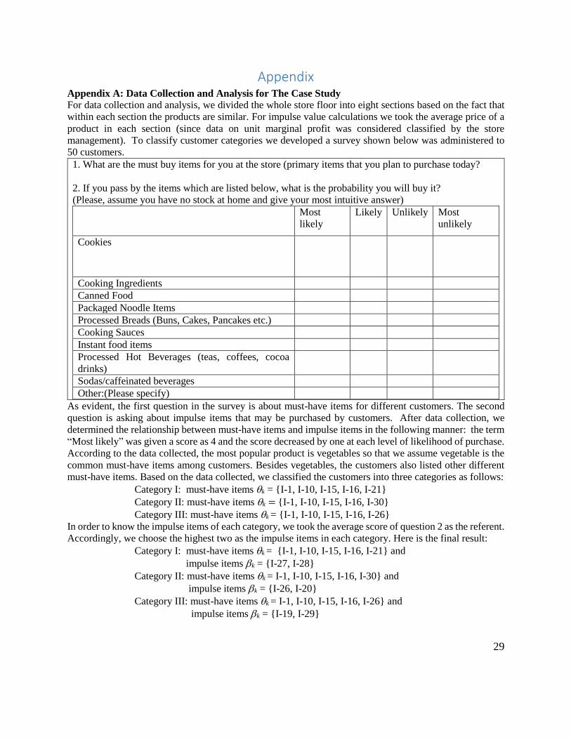
Appendix Appendix A: Data Collection and Analysis for The Case Study

For data collection and analysis, we divided the whole store floor into eight sections based on the fact that

within each section the products are similar. For impulse value calculations we took the average price of a

product in each section (since data on unit marginal profit was considered classified by the store

management). To classify customer categories we developed a survey shown below was administered to

50 customers.

1. What are the must buy items for you at the store (primary items that you plan to purchase today?

2. If you pass by the items which are listed below, what is the probability you will buy it?

(Please, assume you have no stock at home and give your most intuitive answer)

Most

likely

Likely Unlikely Most

unlikely

Cookies

Cooking Ingredients

Canned Food

Packaged Noodle Items

Processed Breads (Buns, Cakes, Pancakes etc.)

Cooking Sauces

Instant food items

Processed Hot Beverages (teas, coffees, cocoa

drinks)

Sodas/caffeinated beverages

Other:(Please specify)

As evident, the first question in the survey is about must-have items for different customers. The second

question is asking about impulse items that may be purchased by customers. After data collection, we

determined the relationship between must-have items and impulse items in the following manner: the term

“Most likely” was given a score as 4 and the score decreased by one at each level of likelihood of purchase.

According to the data collected, the most popular product is vegetables so that we assume vegetable is the

common must-have items among customers. Besides vegetables, the customers also listed other different

must-have items. Based on the data collected, we classified the customers into three categories as follows:

Category I: must-have items k = {I-1, I-10, I-15, I-16, I-21}

Category II: must-have items k = {I-1, I-10, I-15, I-16, I-30}

Category III: must-have items k = {I-1, I-10, I-15, I-16, I-26}

In order to know the impulse items of each category, we took the average score of question 2 as the referent.

Accordingly, we choose the highest two as the impulse items in each category. Here is the final result:

Category I: must-have items k = {I-1, I-10, I-15, I-16, I-21} and

impulse items k = {I-27, I-28}

Category II: must-have items k = I-1, I-10, I-15, I-16, I-30} and

impulse items k = {I-26, I-20}

Category III: must-have items k = I-1, I-10, I-15, I-16, I-26} and

impulse items k = {I-19, I-29}

30

Appendix B: Factorial Design Table

Order No. of Common

must have item

No. of must

have item

No. of Customer

categories

Original

layout value

P-dispersion

value

Simulated annealing

value

1 -1 -1 -1 7.858393026 12.7379251 13.75850427

2 1 -1 -1 8.095413728 13.25179212 13.25179212

3 -1 1 -1 10.86464141 13.46237572 14.96006057

4 1 1 -1 10.74405212 13.68121291 14.64866774

5 -1 -1 1 15.09678 19.89000624 20.95180821

6 1 -1 1 15.2335583 20.38037366 20.38037366

7 -1 1 1 18.42532207 20.55060811 22.20310841

8 1 1 1 18.24589037 20.51638362 21.7539911

9 -1 -1 -1 6.004403361 12.16470795 13.37699877

10 1 -1 -1 5.775112742 12.04285403 12.04285403

11 -1 1 -1 9.346074399 13.09702886 13.75154105

12 1 1 -1 9.390475695 12.99408866 13.30055973

13 -1 -1 1 10.79731313 19.16656682 19.95920438

14 1 -1 1 10.53346102 18.19850416 18.19850416

15 -1 1 1 14.97698015 19.99143632 20.68673789

16 1 1 1 14.61743685 18.99419955 20.83679062

17 -1 -1 -1 6.968725835 10.70626217 12.16132857

18 1 -1 -1 7.243096293 11.51917545 11.51917545

19 -1 1 -1 7.534395382 12.09782749 13.26678582

20 1 1 -1 7.401208033 12.52540583 13.20429611

21 -1 -1 1 15.60475303 20.03961963 20.62580735

22 1 -1 1 15.75946952 21.30508826 21.30508826

23 -1 1 1 17.02334569 20.97462341 22.84578755

24 1 1 1 16.91457791 21.93595426 22.92497507

Appendix C: General Linear Model (Value of Layout 1)

Source

DF Seq SS Adj SS Adj MS F P

Main Effects 3 383.34 383.34 127.78 166.36 0.00

No. of Common must have item 1 0.34 0.344 0.34 0.45 0.51

No. of must have item 1 11.36 11.36 11.363 14.79 0.00

No. of Customer categories 1 371.63 371.63 371.63 483.830 0.00

Residual Error 20 15.36 15.36 0.77

Lack of Fit 4 0.54 0.54 0.13 0.14 0.963

Pure Error 16 14.83 14.83 0.93

Total 23 398.70

R-Sq = 96.15% R-Sq(pred) = 94.45% R-Sq(adj) = 95.57%

31

Appendix D: General Linear Model (Value of Layout 2)

Source

DF Seq SS Adj SS Adj MS F P

Main Effects 3 376.663 376.663 125.554 148.930 0.000

No. of Common must have item 1 1.118 1.118 1.118 1.330 0.263

No. of must have item 1 11.833 11.833 11.833 14.040 0.001

No. of Customer categories 1 363.712 363.712 363.712 431.440 0.000

Residual Error 20 16.861 16.861 0.843

Lack of Fit 4 0.815 0.815 0.204 0.200 0.933

Pure Error 16 16.046 16.046 1.003

Total 23 393.524

R-Sq = 95.72% R-Sq(pred) = 93.83% R-Sq(adj) = 95.07%

Appendix E: General Linear Model (Improvement of Layout 1)

Source DF Seq SS Adj SS Adj MS F P

Main Effects 3 0.56649 0.56649 0.188829 2.37 0.101

No. of Common must have item 1 0.00526 0.00526 0.005256 0.07 0.8

No. of must have item 1 0.01592 0.01592 0.015918 0.2 0.66

No. of Customer categories 1 0.54531 0.54531 0.545313 6.84 0.017

Residual Error 20 1.5947 1.5947 0.079735

Lack of Fit 4 0.0272 0.0272 0.0068 0.07 0.99

Pure Error 16 1.5675 1.5675 0.097969

Total 23 2.16118

R-Sq = 26.21% R-Sq(pred) = 0.00% R-Sq(adj) = 15.14%

Appendix F: General Linear Model (Improvement of Layout 2)

Source DF Seq SS Adj SS

Adj

MS F P

Main Effects 3 0.835 0.835 0.27833 6.61 0.003

No. of Common must have items 1 0.01271 0.01271 0.01271 0.3 0.589

No. of must have item 1 0.35956 0.35956 0.35956 8.54 0.008

No. of Customer categories 1 0.46273 0.46273 0.46273 11 0.003

Residual Error 20 0.84157 0.84157 0.04208

Lack of Fit 4 0.04539 0.04539 0.01135 0.23 0.919

Pure Error 16 0.79618 0.79618 0.04976

Total 23 1.67657

R-Sq = 49.80% R-Sq(pred) = 27.72% R-Sq(adj) = 42.27%

32

Appendix G: Paired T- Test

Original impulse Value ($) p-disp impulse value ($) SA impulse value ($)

12.96791 13.63794 14.09078

10.93634 11.07142 11.8137

9.661359 11.42419 12.21212

10.89489 14.10279 14.22584

12.44378 12.58273 12.95807

14.02544 14.36654 15.12402

15.53402 16.17129 16.7819

13.89049 17.27324 17.77378

10.89121 12.80375 13.12486

13.13141 13.42528 14.46712

14.00723 17.24424 17.78377

10.29376 12.07126 12.37399

22.11665 24.80997 25.27898

14.0312 15.64507 15.96247

17.9396 18.01694 18.69031

15.74383 18.15752 18.72562