TECHNICAL REPORT STANDARD TITLE PAGE

!. Reporl No. 2. Gov..rnmenT Accession No. 3, Rccipi.,nl' s Catalog No.

TX-90/1125-lF 4. Title ond Subtill~ 5. Ra-port Dale

Stopping Sight Distance Considerations at Crest March 19.89 Vertical Curves on Rural Two-Lane Highways in Texas 6. Performing 01gon1zo!ion Code

7, Avrhor1 s) a. Performing Orgonizolion Repor! No.

D.B. Fambro, T. Urbanik II, W.M. Hinshaw, J.W. Hanks Jr. Rese~rch Rep6rt 1125-lF

M.S. Ross, C.H. Tan, and C.J. Pretorius 9, Performing Orgonitotion Nome and Address 10. Work Unit No, I Texas Transportation Institute Texas A&M University 11. Contract or Gron! No. College Station, Texas 77843 Study No. 2~8-87-1125

13. Type of Report and Period Covered

12. Sponsoring Agency Nome and Address and Public Transportation Final - April 1987 State Department of Highways

Transportation Planning Division April 1989

I P.O. Box 5051 14, Sponsoring Agency Codo

Austin, Texas 78763

15. Supplementary Noles

Study Title: Geometric Design Consideration for Rural Roads. This research was funded by the State of Texas.

16. Abstracl

Rehabilitating or upgrading existing two-lane roadways sometimes involves design decisions concerning improved vertical alignment and roadway cross section. These decisions are especially critical. whenever the existing alignment does not meet current standards. In order to make these decisions in a cost-effective manner, the safety and operational effects of alternative crest vertical curve designs must be known, This study attempted to quantify those effects.

In summary, the study concluded that the relationship between available sight distance on crest vertical curves and accidents is difficult to quantify; that the AASHTO stopping sight distance model .is not a good indicator of accidents on two-lane roads; and that when there are intersections within the limited sight distance portions of crest vertical curves, there is a marked increase in accident ·rates. There \\'.'as also no definitive relationship between available sight distance and operating speed on crest vertical curves.

17. Key Words 18. Distribution Stot•menl

Crest Vertical Curves, Stopping Sight No restrictions. This document is Distance, Safety Effects of Design, available to the public through the Geometric Effects of Design National Technical Information Service

5285 Port Royal Road Sorinafield, Vir inia 22161

19. Security Clossif. (of this report) 20. Se<:urity Clas_sif. (of 1hi1 page) 21. No. of Po9os 22. Price

Unclassified Unclassified 129

form DOT F 1700.7 1•-••l

STOPPING SIGHT DISTANCE CONSIDERATIONS AT CREST VERTICAL CURVES

ON RURAL TWO-LANE HIGHWAYS IN TEXAS

by

Daniel B. Fambro, P.E. Assistant Research Engineer

Thomas Urbanik II, P.E. Research Engineer

Wanda M. Hinshaw Assistant Research Statistician

James W. Hanks, Jr., P.E. Assistant Research Engineer

Michael S. Ross Research Assistant

Carol H. Tan Research Assistant

and

Casper J. Pretorius Research Assistant

Research Report 1125-lF Research Study Number 2-8-87-1125

Study Title: Geometric Design Considerations for Rural Roads

Sponsored by the

Texas State Department of Highways and Public Transportation

March 1989

TEXAS TRANSPORTATION INSTITUTE The Texas A&M University System

College Station, Texas 77843-3135

~.

METRIC (SI*) CONVERSION FACTORS

APPROXIMATE CONVERSIONS TO SI UNITS Symbol Whtn You Know Multiply By To And

In ft yd ml

In' ft' yd' ml' ac

oz lb

T

fl oz gal

ft'

Inches feet

yards miles

LENGTH

2.54 0.3048

0.914 1.61

millimetres metres metres kilometres

AREA J.

square Inches square feet square yards square miles acres

645.2 0.0929 0.836 2.59 0.395

millimetres squared metres squared metres squared kilometres squared hectares

MASS (weight)

ounces 28.35 pounds 0.454 short tons (2000 lb) 0.907

fluid ounces gallons cubic feet

VOLUME

29.57 3.785 0.0328

grams kilograms

megagrams

millilitres litres metres dubed

yds cubic yards 0.0765 metres cubed

NOTE: Volumes greater than 1000 l shall be shown In m'.

TEMPERATURE (exact) 1

Fahrenheit 5/9 (after temperature subtracting 32)

Celsius : r temperature

"* SI Is the symbol for the International System of Measurements

Symbol

mm m m km

mm• m• m' km' ha

g kg

Mg

ml l m• m•

•

~

=

N N

• u

APPROXIMATE CONVERSIONS TO SI UNITS Symbol When You Know

mm millimetres m metres m metres km kilometres

Multiply By

LENGTH

0.039 3.28 1.09 0.621

AREA

mm2 millimetres squared 0.0016 m2 metres squared 10. 764

km2 kilometres squared 0.39 ha hectares (10 000 m') 2.53

To Find

Inches feet yards miles

square inches square feet square miles acres

MASS (weight)

g kg

Mg

ml l m• m'

grams 0.0353 kilograms 2.205

megagrams (1 000 kg) 1.103

millilitres litres

metres cubed metres cubed

VOLUME

0.034 ·0.254

35.315 1.308

ounces pounds

short tons

fluid ounces gallons cubic feet cubic yards

TEMPERATURE (exact)

°C Celsius 9/5 (then Fahr0nhelt temperature temperature add 32) .

•f -40 0

I I 11 I 1

11 1 1

-40 -20 •c

•f 98.6 . 212

.. ~. l .1~0. I·'.~. I .~J ~ I I.lo I 60 Jo I 100

37 °C

These factors conform to the requirement of FHWA Order 5190.1A.

Symbol

in ft yd ml

in2

ft' mi 2

ac

oz lb

T

fl oz gal

ft' yd'

•F

\

ABSTRACT

Rehabilitating or upgrading existing two-lane roadways sometimes involves design decisions concerning improved vertical alignment and roadway cross section. These decisions are especially critical whenever the existing alignment does not meet current standards. In order to make these decisions in a cost­effect i ve manner, the safety and operational effects of alternative crest vertical curve designs must be known. This study attempted to quantify those effects.

In summary, the study concluded that the relationship between available sight distance on crest vertical curves and accidents is difficult to quantify; that the AASHTO stopping sight distance model is not a good indicator of accidents on two-lane roads; and that when there are intersections within the limited sight distance portions of crest vertical curves, there is a marked increase in accident rates. There was also no definitive relationship between available sight distance and operating speed on crest vertical curves.

Key Words: Crest Vertical Curves, Stopping Sight Distance, Safety Effects of Design, Geometric Effects of Design

iv

EXECUTIVE SUMMARY

Rehabilitating or upgrading existing two-lane roadways sometimes involves design decisions concerning improved vertical alignment and roadway cross­section. Existing gradelines and available right-of-way on two-lane roadways that were built 40 years ago may make reconstruction to current design standards an expensive undertaking. These costs may be especially high in east and central Texas due to the rolling terrain, numerous existing crest vertical curves, and generally older highways. Thus, in order to make best use of their limited funds, the Texas State Department of Highways and Public Transportation must determine, from both a safety and operational standpoint, under what conditions the selection of new gradelines will be the most effective.

This study attempted to quantify the safety and operational effects of available sight distance at crest vertical curves on two-lane roadways in Texas. From the safety perspective, it was concluded that, even with a relatively large data base, the relationship between available sight distance on crest vertical curves and accidents is difficult to quantify; that the AASHTO stopping sight distance model alone is not a good indicator of accidents on two-lane roads; and when there are intersections within the limited sight distance portions of crest vertical curves, there is a marked increase in accident rates. It should be noted however, that these findings may not hold true outside of the AADT ranges investigated in this study; i.e., 1500 to 6000 vehicles per day. From the operational perspective, there was no definitive relationship between available sight distance and operating speed on crest vertical curves.

From an effectiveness point of view, it was found that for two-lane roadways with shoulders, it generally becomes effective to improve gradelines somewhere between 3900 and 5300 vehicles per day. Below this AADT range, the safety effectiveness of reconstruction is small. For two-lane roadways without shoulders, it generally becomes effective to improve gradelines somewhere between 1500 and 4000 vehicles per day. Below this AADT range, the safety effectiveness of reconstruction is expected to be extremely small. More definitive statements about these low AADT ranges (less than 1500) cannot be made as they were outside the scope of this study.

v

ACKNOWLEDGEMENTS

The research reported herein was performed as a part of a study entitled "Geometric Design Considerations for Rural Roads" by the Texas Transportation Institute and sponsored by the Texas State Department of Highways and Public Transportation. Dr. Daniel B. Fambro and Dr. Thomas Urbanik II of the Texas Transportation Institute served as research co-supervisors, and Mr. Mark A. Marek of the Texas State Department of Highways and Public Transportation served as technical coordinator.

The authors wish to thank Mr. J.L. Beaird, Mr. Harold D. Cooner, and Mr. Frank D. Holzmann of the Texas State Department of Highways and Public Transportation for their technical input and constructive suggestions. Thanks are also extended to Mr. Raymond T. Ellison, SDHPT District I9 in Atlanta; Mr. Kenneth W. Fults, SDHPT District II in Lufkin; and Mr. H. Cornell Waggonner, SDHPT District IO in Tyler for their help in identifying study sites and providing geometric and traffic data for this project.

Thanks are also extended to the numerous research assistants and student technicians at the Texas Transportation Institute who worked on this project. Several of them deserve special recognition--Mr. Gilmer D. Gaston who was responsible for reducing the field data, Ms. Karen M. George who worked extensively with the accident data, Mr. Paul M. Luedtke who checked and rechecked the plan sheets and video records, and Mr. Marc D. Williams who prepared the report's graphics. Special thanks are given to Mss. Robyn Smith and Dana Mixson for their typing skills and Ms. Jeanne Coignet for her technical editing skills, all of which were used extensively in the preparation of this report.

DISCLAIMER

The contents of this report reflect the views of the authors who are responsible for the opinions, findings and conclusions presented herein. The contents do not necessarily reflect the official views or policies of the Texas State Department of Highways and Public Transportation. This report does not constitute a standard, specification, or regulation.

vi

I.

I I.

III.

IV.

TABLE OF CONTENTS

INTRODUCTION . . Background . Objectives . Organization

STATE OF THE ART . . . . AASHTO Design Equations Historical Development ...

Assumed Speed for Design Perception-Reaction Time .. Design Pavement/Stop Conditions Friction Factors Driver Eye Height ... . Object Height ..... .

Sensitivity Analysis .... . Vehicle Speed ..... . Perception-Reaction Time Coefficient of Friction Eye Height Object Height .

Functional Analysis Conclusions ....

SAFETY EFFECTS OF LIMITED SIGHT DISTANCE Safety and Stopping Sight Distance Study Design . . . . Methodology . . . . . . . . . . . Statistical Methods ...... . Results . . . . . . . . . . . . .

Two-Lane Roadways with Shoulders Two-Lane Roadways without Shoulders Four-Lane Divided Roadways Five-Lane Roadways ....... .

Summary . . . . . . . . . . . . . . . .

OPERATIONAL EFFECTS OF LIMITED SIGHT DISTANCE Past Research . . . . . . . Study Design . . . .....

Site Selection Criteria Data Collection .

Study Sites ..... US 59 Study Site US 175 Study Site US 80 Study Site

Data Analysis .... Initial Processing ..... Removal of Partial and Platoon Data

vii

Page

1 1 2 2

3 3 4 4 6 6 7 7 7 8 9 9

11 13 13 16 21

23 23 27 27 29 30 30 40 54 54 55

56 56 57 57 59 63 63 65 65 65 65 65

v.

VI.

VII.

Matching Vehicles ... Statistical Analysis

Results . . . . . . . . . . Frequency Distribution Paired Analysis ... .

Conclusions ....... .

COST EVALUATION OF VERTICAL SIGHT DISTANCE IMPROVEMENTS Development of Typical Cross Sections Identification of Cost Values

Construction Costs ..... Operation Costs . . . . . . . Accident Costs ...... .

Development of Cost Relationships Earthwork . . . . . . . . . . Pavement/Stabilized Base .. Detour Construction and Maintenance Delay . . . . . . Traffic Handling ........ .

Cost Analysis ............ .

BENEFIT-COST ANALYSES OF VERTICAL SIGHT DISTANCE IMPROVEMENTS Calculation of Benefits ....... . Benefit-Cost Analysis ........ .

Two-Lane Roadways with Shoulders Two-Lane Roadways without Shoulders Benefit-Cost Ratio ....... .

Conclusions

SUMMARY AND CONCLUSIONS

65 65 66 66 71 75

78 78 79 79 80 81 82 82 84 85 86 86 86

92 92 97 99

100 101 104

105

REFERENCES . . . . . . 106

APPENDIX A . . . . . . . . . . . . . . . . . . . . 110 Geometric and Accident Data for Individual Roadway Segments

viii

1

2

3

4

5

6

7

LIST OF TABLES

History of AASHTO Stopping Sight Distance Parameters

Values Used in the Sensitivity Analysis of AASHTO Design Values ....... .

Comparison of Perception-Reaction and Braking Distance Between 30 mph and 70 mph .....

Accident Rates on Two-Lane Curved Sections for AADT Volumes from 5,000 to 9,900 and Grades Above and Below 3 Percent

Freeway Accident Rates for Different Types of Crest and Sag Vertical Curves ............. .

Frequency and Percentage of Two-Lane Roadway with Shoulder Segments within Specified AADT Levels ......... .

Frequency and Percentage of Limited Stopping Sight Distance on Two-Lane Roadway with Shoulder Study Segments

8 Frequency of Total Intersecting Roads and Intersections within Limited Sight Distance Sections on Two-Lane

Page

5

8

11

24

25

31

33

Roadways with Shoulders . . . . . . . . . . . . . . . . . 37

9 Summary of Regression Analysis for the Dependent Variable, Logarithm of Accidents Per Mile on Two-Lane Roadways with Shoulders . . . . . . • • . . . . . . . . . . 37

10 Summary of Regression Analysis for the Dependent Variable, Logarithm Accident Rate per mvm on Two-Lane Roadways with Shoulders . . . . . . . . . . . . . . . . . 38

11 Regression Coefficients for Analysis of Criterion of Minimum Sight Distance for 55 mph (450 ft) on Two-Lane Roadways with Shoulders . . . . . . . . . . . 39

12 Estimated Values of Accidents Per Mile on Two-Lane Roadways with Shoulders . . . . . . . . . . . . . 40

13 Frequency of Segments by AADT and Percent Limited Sight Distance (450 ft) on Two-Lane Roadways without Shoulders 42

14 Frequency and Percentage of Limited Stopping Distance on Two-Lane Roadways without Shoulder Study Segments 43

15 Summary of Regression Analysis Using 325-Foot Criterion for the Dependent Variable, Logarithm of Accidents Per Mile on Two-Lane Roadways without Shoulders . . . . . . . . . . 45

ix

16 Summary of Regression Analysis Using the 450-Foot Criterion for the Dependent Variable, Logarithm of Accidents Per Mile on Two-Lane Roadways without Shoulders . . . . . . . . . 47

17 Summary of Regression Analysis Using 550-Foot Criterion for the Dependent Variable, Logarithm of Accidents Per Mile on Two-Lane Roadways without Shoulders . . . . . . . . . 47

18 Regression Coefficients from the Analysis of Logarithm of Accidents Per Mile on Two-Lane Roadways without Shoulders 49

19 Estimated Accidents Per Mile for AADT = 2000 and Stopping Sight Distance Criterion = 450 feet on Two-Lane Roadways without Shoulders . . . . . . . . • . . . . . . 50

20 Characteristics of Crest Vertical Curves Selected as Field Study Sites . . . . . . . . . . . . . . . 63

21 Assumed Cross-Section Design Variables for Analysis 79

22 Cost in Relation to Roadway Cross-Sectional and Curve Characteristics . . . . . . . . . . . . . . . . 82

23 Estimated Earthwork Quantities in Cubic Yards Existing A and K Values to Achieve a K min = 150 . . • . . . . . . . . 83

24 Pavement/Stabilized Base Quantities Required By Existing Algebraic Difference in Grade and Roadway Type to Achieve a K Min = 150 . . . . . . . . . . . . . . . . 84

25 Estimated Detour Construction and Maintenance Cost 85

26 Estimated Delay Cost Due to Construction Activities 86

27 Estimated Realignment Cost for Two-Lane Roadways without Shoulders/Crest Curve . . . . . . . . . . . . . . . 87

28 Estimated Realignment Cost for Two-Lane Roadways with Shoulders/Crest Curve . . . . • . . . . . . . 88

29 Estimated Realignment Cost for Four-Lane Divided Roadways/ Crest Curve . . . . . . . . . . . . . . . . . . . . . 89

30 Estimated Realignment Cost for Five-Lane Roadways with Shoulders/Crest Curve . . . . . . . . . . . . . . . . 90

31 Estimated Realignment Cost for Five-Lane Roadways with Curb and Gutter/Crest Curve . . . . . . . . . 91

32 Total Costs of Traffic Accidents on Rural, Undivided Roadway • . . . . . . . • . . . . . . . . . . . . . • . . . 92

x

33 Annual Savings per Mile for Two-Lane Roadways with Shoulders, Minimum Limited SSD = 450 ft., Maximum Limited SSD per Section = 15 percent . . • . . . . . ... 94

34 Annual Savings per Mile for Two-Lane Roadways without Shoulders, Minimum Limited SSD = 325 ft., Maximum Limited SSD per Section = 25 percent ............ 95

35 Annual Savings per Mile for Two-Lane Roadways without Shoulders, Minimum Limited SSD = 450 feet ......... 96

xi

I

2

3

4

5

6

7

8

9

IO

LIST OF FIGURES

Sensitivity of Required Length of Crest Vertical Curve Changes in Driver Perception-Reaction Time ..... .

Sensitivity of Required Length of Crest Vertical Curves to Changes in Coefficient of Friction .•......

Sensitivity of Required Length of Crest Vertical Curves to Changes in Driver Eye Height ....... .

Sensitivity of Required Length of Crest Vertical Curves to Changes in Object Height ............ .

Available Sight Distance as a Function of Curve Geometry, A = 2 . . . . . . . . . . . . . . . Available Sight Distance as a Function of Curve Geometry, A = 4 . . . . . . . . . . . . . . . Available Sight Distance as a Function of Curve Geometry, A = 6 . . . . . . . . . . . . . Available Sight Distance as a Function of Curve Geometry, A = 8 . . . . . . . . . . . .

. .

.

.

. . Length of Roadway with SSD Less Than 450 Feet as a Function of Crest Curve Geometry . . . . . . . . . . . . . . . . .

Relationship Between Accidents Per Mile and Annual Average Daily Traffic, Two-Lane Roads with Shoulders ..... .

Page

IO

I2

I4

I5

17

. IS

. I9

20

22

32

II Relationship Between Accidents Per Mile and Percent of Roadway with SSD Less Than 450 Feet, Two-Lane Roads with Shoulders . . . . . . . . . . . . . . . . . . . . . . . . . 34

12 Relationship Between Annual Average Daily Traffic and Percent of Roadway with SSD Less Than 450 Feet, Two-Lane Roads with Shoulders . . . . . . . . . . . . . . . 34

I3 Relationship Between Accident Rate (mvm) and Annual Average Daily Traffic, Two-Lane Roads with Shoulders • . . . . . 35

14 Relationship Between Accident Rate (mvm) and Percent of Roadway with SSD Less Than 450 Feet, Two-Lane Roads with Shoulders . . . . . . . . . . . . . . . . . . . . . . . . 35

I5 Relationship Between Accidents Per Mile, Percent of Roadway with SSD Less Than 450 Feet, and Number of Intersections, Two-Lane Roads with Shoulders . . . . . . • . . . . . . . . 4I

xii

16 Relationship Between Percent of Roadway with SSD Less Than 450 Feet and Annual Average Daily Traffic, Two-Lane Roads with Shoulders . . . . . . . . . . . . • . . . . . . . . . 41

17 Relationship Between Accidents Per Mile and Annual Average Daily Traffic, Two-Lane Roads with Shoulders . . . . . . . 44

18 Relationship Between Accidents Per Mile, Percent of Roadway with SSD Less Than 325 Feet, and Number of Intersections, Two-Lane Roads with Shoulders . . . . • . . . . . . . . . . 44

19 Relationship Between Accidents Per Mile, Percent of Roadway with SSD Less Than 450 Feet, and Number of Intersections, Two-Lane Roads without Shoulders . . . . . . . . . . . . . . 46

20 Relationship Between Accidents Per Mile, Percent of Roadway with SSD Less Than 550 Feet, and Number of Intersections, Two-Lane Roads without Shoulders . . . . . . . . . . . . . 48

21 Relationship Between Accident Rate (mvm) and Annual Average Daily Traffic, Two-Lane Roads without Shoulders . . • . . 51

22 Relationship Between Accident Rate (mvm), Percent of Roadway with SSD Less Than 325 Feet, and Number of Intersections, Two-Lane Roads without Shoulders . . • . . . . . . . . . . . 51

23 Relationship Between Accident Rate (mvm), Percent of Roadway with SSD Less Than 450 Feet, and Number of Intersections, Two-Lane Roads without Shoulders . . . . . . . . . . . . . . 52

24 Relationship Between Accident Rate (mvm), Percent of Roadway with SSD Less Than 550 Feet, and Number of Intersections, Two-Lane Roads without Shoulders . . • . . . . . . . . 52

25 Study Sites (Two-Lane Roads without Shoulders) Located on the Same Control-Section . . . . • . 53

26 Types of AASHTO Crest Vertical Curves 58

27 Typical Study Site Set-Up Using a Tangent Section as the Control . . . . 62

28 US 59 Study Site Set-Up 64

29 US 175 Frequency Distribution Plots for Day vs Night 68

30 US 175 Frequency Distribution Plots for Cars vs Trucks 69

31 US 175 Frequency Distribution Plots for East vs West 70

32 US 59 Frequency Distribution Plots for Cars vs Trucks by Station . . . . . . . . . . . . . . . . . . . . . . 72

xiii

33

34

35

36

37

Results From the US 175 Eastbound Study Site

Results From the US 175 Westbound Study Site

Results From the US 59 Northbound Study Site

Results From the US 59 Southbound Study Site

Benefit/Cost Ratio = 1, Two-Lane Roadways with Shoulders, Minimum Limited SSD = 450 ft. . . . . . . . . ....

xiv

73

74

76

77

98

I. INTRODUCTION

Rehabilitating or upgrading existing two-lane roadways sometimes involves design decisions concerning improved vert i ca 1 alignment and roadway cross section. Existing gradelines and available right-of-way on two-lane roadways that were built 40 years ago may make reconstruction to current design standards an expensive undertaking. These costs may be especi.ally high in the rolling terrain found in east and central Texas due to the numerous crest vertical curves and generally older highways. Thus, in order to make the best use of their 1 imited funding, the Texas State Department of Highways and Public Transportation (TSDHPT} must determine, from both a safety and operational standpoint, under what conditions the selection of new gradelines is the most beneficial.

Currently, the Federal Highway Administration (FHWA} will not approve new construction or reconstruction of a federal aid project unless the design speed of the entire roadway, including crest vertical curves, either meets or exceeds the posted speed 1 imi t on the facility. In a few speci a 1 cases, however, a design exception may be granted. To obtain a design exception, it is necessary to prove that the existing or proposed geometric design feature does not have a negative impact on the safety or operation of the roadway. The process of procuring a design exception is difficult given the large amount of data required, the lack of information on what constitutes a significant problem, and the unknown outcome of the results.

Failure to resolve the issue of design speed versus posted speed could result in costly regrading for rehabilitation projects, as well as unjustifiable construction, environmental, and economic costs on some new roadways. In light of these pro bl ems, the TSDHPT has contracted with the Texas Transportation Institute (TTI} to determine when, from an economical, safety, and operational standpoint, design exceptions should be sought.

Background

The primary measure of design adequacy for crest vertical curves is the amount of stopping sight distance (SSD} provided in relation to the design speed of the roadway. The American Association of State Highway and Transportation Officials (AASHTO} defines SSD as the length of roadway required for a vehicle traveling at or near the design speed of the roadway to stop before reaching a stationary object in its path (1). SSD is broken down into brake reaction time (the time measured from the instant of object detection to the instant the brakes are applied} and braking distance (the distance required for the vehicle to come to a complete stop}.

The amount of stopping sight distance required on vertical curves, for a given speed, is dependent upon the eye height of the driver and the height of the object that must be detected. In the 1940s these values were set at 4.5 feet and 4.0 inches, respectively (i}. In 1965, prompted by decreasing vehicle sizes, the value for driver eye height was lowered to 3.75 feet, and the value for object height was raised to 6.0 inches (~}. Decreasing vehicle sizes necessitated a further reduction in driver eye height to 3.5 feet in 1984 (1).

1

As some of these design values were lowered, the net required length of vertical curve necessary to provide recommended SSD increased. These newer values, 3.5 feet and 6.0 inches, require a vertical length approximately 5 percent greater than that used prior to 1984 (!). The problem is that many of the two-lane roadways in the state were built even before the 1965 changes were put into effect. This change in criteria since construction means that the roadway's existing geometric design features may not meet the current standards. Therefore, if a vertical curve does not meet the current stopping sight distance criteria for the design speed of the roadway, it would be necessary to determine if limitations of the existing design have any significant effect on the safety or operation of the roadway. With this information, it is possible to develop guidelines for use by the TSDHPT in selecting the most cost-effective design treatment for federal aid projects.

Objectives

The principle objective of this research was to determine for a variety of cross sections the cost effectiveness of maintaining design speeds for crest vertical curves greater than or equal to the posted speed limit on the roadway. In order to accomplish this principle objective, a review of the literature, a sensitivity and functional analysis of the SSD equations, an evaluation of the safety and operations of each cross section, and an economic analysis of the various alternative designs were conducted.

Organization

This report presents the results of this research and is organized into seven chapters. Chapter I describes the problem and background, research objectives, and organization of the report. Chapter II contains the literature review and the results of the sensitivity and functional analyses. The results of the safety study and the operational study are described in Chapter III and Chapter IV, respectively. Chapter V describes procedures for conducting a cost evaluation while Chapter VI describes a method of doing a benefit-cost analysis. A Summary and Conclusion of this research are presented in Chapter VII. Appendix A contains geometric and accident data for individual roadway segments.

2

II. STATE OF THE ART

One of the most important requirements in highway design is to provide adequate stopping sight di stance at every point a 1 ong the roadway. Crest vertical curves limit available sight distance; however, when designed in accordance with AASHTO criteria, adequate stopping sight distance should be available at all points along the curve. Therefore, the design of crest vertical curves is dependent upon stopping sight distance. The following section describes the AASHTO design equations and the historical development of the design parameters used in the calculation of stopping sight distance and length of crest vertical curves. Included in this section are sensitivity and functional analyses of each of these design parameters.

AASHTO Design Equations

Stopping sight distance is calculated using basic principles of physics and the relationships between various design parameters. AASHTO defines stopping sight distance as the sum of two components, brake reaction distance (distance traveled from the instant of object detection to the instant the brakes are applied) and the braking distance (distance required for the vehicle to come to a complete stop). SSD can be expressed by the following equation:

SSD = I.47Vt + 1- [1] 30f

where, SSD = stopping sight distance (feet);

v = design or initial speed (miles per hour);

t = driver perception-reaction time (seconds); and

f = friction between the tires and the pavement.

The minimum length of a crest vertical curve is controlled by required stopping sight distance, driver eye height, and object height. This length is such that stopping sight distance calculated by Equation 1 is available at all points along the curve. AASHTO uses the following formulas for determining the required length of a crest vertical curve:

3

\_ - ----- --

where,

L

L

L

s A

h,

h,

=

=

=

=

Historical Development

100( 2h1 + 2h2)2

2S - 200 ( h, + h,t A

When S < L

When S > L

length of vertical curve (feet);

sight distance (feet);

algebraic difference in grade (percent);

eye height above the roadway surface (feet); and

object height above the roadway surface (feet).

[2]

[3]

Over the past 50 years, design parameters for crest vertical curves have been addressed in several AASHO and AASHTO publications. The fundamental principles of highway design were discussed in textbooks as early as 1921; however, it was not until 1940 that seven documents were published by AASHTO which formally recognized policies on certain aspects of geometric design. These seven policies were reprinted and bound as one volume entitled Policies on Geometric Highway Design (l) in that same year. These policies were revised and amended in a 1954 document, A Policy on Geometric Design of Rural Highways (~). In 1965 and again in 1970 this document was revised and republished under the same title and, because of the color of its cover, was referred to as the "Blue Book" (1,.§.). The current comprehensive document is entitled A Pol icy on Geometric Design of Highways and Streets, 1984 which is commonly referred to as the "Green Book" (l). The changes in the standards of the design parameters for stopping sight distance and crest vertical curve design which have occurred from 1940 to the present are summarized in Table 1 and discussed below.

Assumed Speed for Design. The use of full design speed in calculating stopping sight distance was first adopted by AASHTO in 1940. In 1954, AASHTO approximated the assumed speed on wet pavements to be a percentage varying from 85 to 95 percent of the design speed based on the assumption that most drivers will not travel at full design speed when pavements are wet. In 1965, AASHTO changed the approximated speed on wet pavements to be a percentage varying from 80 to 93 percent of the design speed. Khasnabis and Tadi, however, questioned the premise that drivers tend to drive at 1 ower speeds on wet pavement and suggested using design speed or an intermediate speed (average of design speed and assumed speed) to compute SSD (~).

4

TABLE 1. History of AASHTO Stopping Sight Distance Parameters.

1940 1954 1965 1970 1984 Parameter A Polley on Sight A Policy on Geometric A Policy on Geometric Policy of Geometric Design Policy of Geometric Design

Distance for Highways Design - Rural Highways Design - Rural Highways of Highways and Streets of Highways and Streets

Design Speed Design Spe'ed Speeds 85 to 95 Speeds 80 to 93 Min. - speeds 80 to 93 Min. - speeds 80 to 93 percent of design percent of design percent of design speed percent of design speed speed speed Des. - design speed Des. - design speed

Percept ion- Variable: Reaction Time 3.0 secs at 30 mph 2. 5 seconds 2. 5 seconds 2.5 seconds 2.5 seconds

2.0 secs at 70 mph

<n Design Pavement/ Dry Pavement Wet Pavement Wet Pavement Wet Pavement Wet Pavement Stop Locked-wheeled locked-wheeled Locked-wheeled Locked-wheeled Locked-wheeled

Stop Stop Stop Stop Stop

Friction Ranges from Ranges from Ranges from Ranges from Slightly lower at higher Factors 0.50 at 30 mph 0.36 at 30 mph 0.36 at 30 mph 0.35 at 30 mph speeds than 1970

to 0.40 at 70 mph to 0.29 at 70 mph to 0.27 at 70 mph to 0.27 at 70 mph values

Eye Height 4.5 feet 4.5 feet 3.75 feet 3.75 feet 3.50 feet

Object Height 4.0 inches 4.0 inches 6.0 inches 6.0 inches 6.0 inches

In the 1984 AASHTO pol icy (l), a range of design speeds, defined by a minimum and a desirable value, was given for computing stopping sight distance. The minimum value was based on an assumed speed for wet conditions, while desirable values were based on design speed. Interestingly, AASHTO notes that "recent observations show that many operators drive just as fast on wet pavements as they do on dry." NCHRP 270 "Parameters Affecting Stopping Sight Distance" (I) concurred that design speed should continue to be used in calculating required stopping sight distance.

Perception-Reaction Time. Perception-reaction time is the summation of brake reaction time and perception time. Brake reaction time was assumed as one second in 1940 (~); since then, there have been no changes in the recommended value for brake reaction time. Total perception-reaction time, however, ranged from two to three seconds, depending upon design speed. In 1954, the "Blue Book" (~) adopted a policy for a total perception-reaction time of 2.5 seconds for all design speeds. The "Blue Book" (~) stated "available references do not justify distinction over the range in design speed." The "available references" were uncited; therefore, the reason for this change is somewhat vague.

NCHRP 270 (I) conducted two separate studies on perception-reaction time, using surprise and expected objects in the roadway. The results of the study found a perception-reaction time of 2.4 seconds to be a reasonable value. Since the value of 2.4 seconds was so close to the current 2.5 seconds, the study recommended the continued use of 2.5 seconds for total perception-reaction time. A study by Hooper and McGee (2.) suggested a perception-reaction time of 3 .2 seconds. This value was calculated by summing component reaction times, including latency, eye movement, fixation and recognition, decision, and brake reaction times. Hooper and McGee (2.) cited another recent study which recommended the use of a range of perception-reaction times from 2.5 seconds at a speed of 25 miles per hour to 3.5 seconds at a speed of 85 miles per hour. These recommendations have not been adopted.

In the above discussion of perception-reaction times there is no consideration given to the di stri but ion of the characteristics of drivers. Khasnabis and Tadi (~) indicated that statistics show there has been a change in the driver population between 1960 and 1980. There is now a more even distribution between male/female drivers and a greater percentage of elderly and teenage drivers. The study suggested more research should be done to determine if any relationship exists between reaction time and both sex and age. Such a relationship would be extremely important if, as expected, the percentage of elderly drivers continues to increase.

Design Pavement/Stop Conditions. The basic assumption in calculating braking distances since the 1940s has been that of locked-wheel tires on wet pavement throughout the braking maneuver. Lower coefficient of friction values are found and longer braking distances result on wet pavements when compared to dry pavements; thus, design is governed by wet conditions.

NCHRP 270 (I) stated that "locked-wheel stopping is not desirable and it should not be portrayed as an appropriate course of action." Instead, NCHRP 270 (I) assumed a controlled stop in calculating the braking distance. A controlled stop is defined as a stop in which the driver "modulates his braking without

6

losing directional stability and control." A numerical integration procedure was developed for calculating the braking distance assuming a controlled stop. The study supported the assumption of a controlled stop, stating that a driver will be able to better control the vehicle in a controlled stop situation, and thus will avoid a locked-wheel situation.

Friction Factors. Friction values should be characteristic of variations in vehicle performance, pavement surface condition, and tire condition. As can be noted in Table 1, for each publication, the friction factors were revised in accordance with the prevailing knowledge of the time. A Policy on Sight Distance for Highways, 1940 (l), utilized a factor of safety of 1.25 to allow for the variations due to a lack of extensive field data. As more studies were completed, empirical friction factors were utilized in design. Friction factors decreased with an increase in speed in all cases.

Khasnabis and Tadi (~) suggested that AASHTO's recommended friction values may not reflect the worst or nearly worst pavement conditions. Their study showed that experiments with "Wet Plant Mix" pavement have produced the lowest friction values. Researchers felt that the new stopping sight distances should be calculated with the "Wet Plant Mix" friction values, "since the stopping sight distance should be derived for 'worse than average' conditions."

Driver Eye Height. The design value of driver eye height is based upon a value which most of the current vehicle driver fleet exceeds. As seen in Table 1, this design parameter has decreased from 54 to 40 inches over a period of approximately 44 years. The change in eye height can be attributed to the increase in the number of small vehicles, vehicle design change,s, different seat angle designs, and head rotation. At the time of each AASHTO publication, the eye height was based on the prevailing distribution of drivers and vehicles. The most significant decrease in driver eye height took place between 1954 and 1965, when the eye height changed from 54 to 45 inches. Although the trend seems to be a continuing decrease in eye height, most studies (I,10) now state that the eye height will not decrease significantly in the future.

Object Height. The issue of which object height should be used in calculating stopping sight distance has been a controversial subject for many years. The fluctuations in object height from 1940 to the present are shown in Table 1. In a 1921 highway engineering textbook, the object was set to the driver eye height, 5.5 feet (ll). A four-inch object height was adopted in 1940 by AASHTO as an "average" control value (l). This value was actually selected on the basis of a compromise between object height and required vertical curve length (li). In 1954, the four-inch object height was justified as "the approximate point of diminishing returns" (Q). An object height of six inches was then adopted in 1965 (Q). The use of the six-inch object height is not well supported in the 1965 literature. In fact, the exact paragraph used in 1954 to justify a four-inch object height was also used to justify the six-inch object height in 1965 (J, Q).

The 1984 "Green Book" (l) considered a six-inch object height to be "representative of the lowest object that can create a hazardous condition and be perceived as a hazard by a driver in time to stop before reaching it." NCHRP 270 (I) recommended reducing the object height to four inches, reasoning that

7

with the number of smaller vehicles increasing, the average clearance level is al so decreasing. NCHRP 270 (I) al so stated that a four-inch object is less likely to damage or deflect a vehicle than the current six-inch object. Therefore, a vehicle is more likely to safely pass over a four-inch object than a six-inch object.

Sensitivity Analysis

As discussed in the previous section, there are six variables that are utilized in the basic AASHTO design equations to determine SSD at crest vertical curves:

I. Vehicle speed; 2. Perception-reaction time; 3. Coefficient of friction; 4. Eye height; 5. Object height; and 6. Algebraic difference in grades.

It is important to know the effect of changing the value of a design parameter upon other parameters and the overall change in stopping sight distance and crest vertical curve design. The first five of these parameters are specified or regulated by highway engineers; the last, the algebraic difference in grade, is the result of local conditions. The sensitivity of vehicle speed, perception­reaction time, coefficient of friction, eye height, and object height is discussed in the following sections. Most of the sensitivity analyses were conducted by holding all variables except the parameter under study at the value recommended by current AASHTO policy. Table 2 presents the AASHTO recommended value for each variable in the analysis.

TABLE 2. Values Used in the Sensitivity Analysis of AASHTO Design Values.

Variable

Vehicle Speed and Coefficient of Friction

Perception-Reaction Time Driver Eye Height Object Height Algebraic Difference in Grade

8

Constant

70 mph 60 mph 50 mph

2.5 seconds 3.5 feet 0.5 feet 2 percent 4 percent 6 percent 8 percent

0.26 0.25 0.30

Vehicle Speed. Vehicle travel speed is an extremely sensitive parameter in the determination of required stopping sight distance. Farber (IO} indicated that small deviations in speed are equivalent to large deviations in stopping sight distance. For example, at 60 mph, each one-mile-per-hour change in speed results in a 17-foot change in SSD. This increase is significant in the selection of which value to use for vehicle speed in the calculation of SSD.

Use of a design or intermediate speed, as suggested by Khasnabis and Tadi (~), instead of assumed speed would result in greater stopping sight distances. The greater stopping sight distances, in turn, result in longer crest vertical curves. Khasnabis and Tadi rn> analyzed the sensitivity of various design parameters by finding the change in the rate of vertical curvature (K value} as opposed to finding the change in vertical curve length. At a design speed of 70 mph, a 6 mph speed differential causes a 62 percent increase in the K value. An increase in the K value results in an increase in SSD. Woods (I3} showed that a 10 percent increase in vehicle operating speed yielded an increase of about 40 percent in crest vertical curve length for speeds between 40 and 65 mph.

Perception-Reaction Time. As mentioned previously, perception-reaction(p­r} time is currently set at 2.5 seconds for all design speeds(~}. Woods (ld} observed that any change in p-r time is actually a change in the distance travelled at the design speed. Glennon (14} observed that for "higher speeds, the stopping sight distance is significantly increased for a one-second increase" in p-r time. Farber (IO} found similar results, indicating that at higher speeds "a small increase in reaction time has a substantial effect on stopping sight distance."

Figure I illustrates required lengths of vertical curve based on various driver perception-reaction times, vehicle speeds of 50, 60, and 70 mph and algebraic differences in grades of 2, 4, 6, and 8 percent. In all cases, an increase in p-r time results in an increase in vertical curve length. At higher speeds, a change in p-r times has a greater impact on vertical curve length than at lower speeds. This effect is most obvious with larger algebraic differences in grade. The differences in curve length between the 50, 60, and 70 mph also increase as both p-r time and algebraic difference in grade increase.

On the other hand, Hooper and McGee (~} stated that SSD is less sensitive to changes in p-r time at higher speeds. Their reasoning being "the braking distance component accounts for a greater portion of the total distance as speed increases." In other words, at higher speeds, vehicles travel a much farther distance while braking than during perception and reaction. A comparison of required braking distance for design speeds between 30 mph and 70 mph is shown below in Table 3 using p-r time of 2.5 seconds. At 30 mph, 56 percent of the total stopping sight distance is composed of the distance traveled during p-r time. This percentage decreases as vehicle speed increases. At 70 mph, the distance traveled during p-r time is only 3I percent of the total stopping sight distance.

9

7000

6000

.ti .;

8 5000

Ol 0

"€ ~

4000

~ 00 a 3000 ~ 0 .:;

! 2000

1000

0 1.5

7000

6000

.ti cf' 5000 ~. u·

~ ~

4000

~ 3000

'il .:; ! 2000

1000

+ V=50mph

-+- V=60mph

*" V:?Omph

A=2

:llE llE ~~ * :!IC )!( :!IE )IE 11(

* I

2 2.5 3

Driver Perception-Reaction Time, sec.

e e e

+ V=fiOmph

-+- V = 60 mph

"""'*"- V=?Omph

A= 6

e e e

7000

6000

.ti .;

~ 5000

u Ol

-~ >

4000

~ 00 a 3000

~ 0

~ 2000

j 1000

0

3.5 1.5

7000

6000

.ti .;

8 5000

Ol 0

"€ ~

4000

<;;;

a 3000

'il .:; !'2000

1000

+ V=50mph

-+- v .. aomph

*" V=?Ompb ... =.

e -() e e e e

() e e e

2 2.5 3

Driver Perception-Reaction Time, sec.

+ V=50mph

-t- V = 60 mph

"""'*"- V=70mph

A= e

o~~~~~~~~~~~~~~~~~~ 0 1.5 2 2.5 3 3.5 1.5 2 2.5 3

Driver Perception-Reaction Time, sec. Driver Perception-Reaction Time, sec.

Figure 1. Sensitivity of Required Length of Crest Vertical Curve to Changes in Driver Perception-Reaction Time.

10

3.5

3.5

Speed Total SSD

(mph) (ft)

30 196 40 314 50 462 60 634 70 841

TABLE 3. Comparison of Perception-Reaction and Braking Distance Between 30 mph and 70 mph.

Distance Traveled Percentage Distance Traveled During P-R Time of SSD During Braking

(ft) (ft)

110.3 56 85.7 147.0 47 166.7 183.8 40 277.8 220.5 35 413 .8 257.3 31 583.3

Percentage of SSD

44 53 60 65 69

Coefficient of Friction. Tire-pavement friction appears to be the most sensitive parameter in determining SSD. Farber (10) indicated "as design travel speed increases so does the sensitivity of stopping sight distance to pavement friction." He found that at 50 mph, SSD wi 11 decrease nine feet with a 0. 01 decrease in friction coefficient. Woods (15) stated that the tire-pavement friction variable is "by far the most critical value in the determination of vertical curve length." Woods (.Q, li) showed, for "f" values near 0.35, an increase of about four percent in vertical curve length for each 0.01 decrease in pavement friction.

Curve lengths increase at a greater rate at lower friction values; thus, the greatest level of sensitivity is at the lower end of the friction scale. For low "f" values, near 0.10, a change of 0.01 in the friction factor causes a 20 percent change in vertical curve length. Figure 2 illustrates the effect of coefficient of friction on vertical curve length for various algebraic differences in grade. As with p-r time, the differences in curve length between speeds increase as algebraic difference in grade increase.

Friction values are al so affected by changes in temperature. Hi 11 and Henry (16) ascertained that a temperature increase of 10 degrees centigrade can cause a pavement's friction value to decrease by more than 0.01. Thus, a change in pavement temperature can result in an increase in SSD. High temperatures are not normally a problem on wet pavements.

11

22000

20000

.::: 18000

oJ > 18000 M

= u OI 14000

<.) ·:: t 12000 > ..: 10000 e u ._

8000 0

-s .. 8000 .:i 4000

2000

0 0

22000

20000

.::: 18000

oJ > 16000 M

= u OI 14000

<.)

·:: t 12000 > ..: e 10000 u '(; 8000 -s .. .:i 8000

4000

2000

0 0

+ V = &O mph

+ V z IO mph.

* v = '70 mph

••• .::: oJ i: = u OI .Jl t > ..: e u ..... 0

-s .. ii

..J

0.1 0.2 0.3 o .• Coefficient of Friction, f

+ V=OOmpb

+ 'f'•IOmpb

* 1' s 70 mph

••• .::: oJ > M = u OI

<.) ·:: t > ..: e u ..... 0

.:; .. ii

..J

0.1 0.2 0.3 o.• Coefficient of Friction, f

22000

20000

18000

18000

14000

12000

10000

8000

8000

4000

2000

0 0

22000

20000

18000

18000

14000

12000

10000

8000

1000

4000

2000

0 0

+ V1:50mph

+ V=SOmpb

* Vc?Omph

• ••

0.1 0.2 0.3

Coefficient of Friction, f

0.1 0.2

+ V•&Ompb

-+- V • 90 mph

* Vs70mph

• ••

0.3

Coefficient of Friction, f

Figure 2. Sensitivity of Required Length of Crest Vertical Curves to Changes in Coefficient of Friction.

12

0.4

0.4

Eye Height. Many studies have been conducted on the sensitivity of eye height. AASHTO (l) indicated that the change in eye height from 3.75 feet to 3.5 feet has the effect of "lengthening minimum crest vertical curves by approximately five percent, thereby providing about 2. 5 percent more sight distance." Farber (10) generalized the sensitivity by stating "a six-inch change in eye height will produce about a five percent change in sight distance." Khasnabis and Tadi (~) found that a three-inch reduction in eye height (3.75 feet to 3.5 feet) causes approximately a 5.3 percent increase in K values (for object heights of 0. 5 feet and 0. 25 feet) . 01 sen et. a 1 . (l) eva 1 uated the difference between a 40-inch eye height and a 42-inch eye height. The difference in curve length was found to be about three percent, with the 40-inch eye height requiring longer sight distance than the 42-inch eye height.

Woods (13, 12) indicated that stopping sight distance is relatively insensitive to changes in driver eye height. A 2.3 percent change in vertical curve length results from each 0.1 foot reduction in the design driver eye height. An 11.5 percent change in the minimum length of vertical curve would result over the range from 3.5 feet to 3.0 feet. The consensus among all of these researchers is that a moderate reduction in driver eye height results in small change in vertical curve length and SSD; this observation is supported by Figure 3. For large algebraic differences and at higher speeds, however, the reduction in eye height increases vertical curve length noticeably. Thus, even though the percentage is small, the additional length of curve may be quite long.

Object Height. Object height sensitivity has also been researched substantially. AASHTO (l) declared that "using object heights of less than six inches for stopping sight distance calculations results in considerably longer crest vertical curves." By decreasing the object height from six inches to zero, the vertical curve length would increase by about 85 percent. Farber (1Q) found sight distance to be considerably more sensitive to object height than to eye height. Khasnabis and Tadi (~) found a reduction in object height from six to three inches caused an 18.6 percent increase in the K factor, and a reduction in object height from three to zero inches caused a 61 percent increase in the K factor. NCHRP 270 (l) also analyzed the results of a reduction in object height from three inches to zero. The researchers ascertained that a zero-inch object height requires about ten percent more vertical curve length than present AASHTO standards.

Figure 4 demonstrates the increase in vertical curve length that results from 1 oweri ng object height va 1 ues. There does not appear to be a 1 arge increase in curve length when decreasing object height incrementally for algebraic difference of grades of 4 percent and lower. For algebraic difference of grades greater than 4 percent, the increase in curve length, especially when using one­and zero-inch object heights is more pronounced. Thus, it would appear that object height is more sensitive for high values of algebraic differences in grade, especially around values of one inch or lower.

13

8000 8000 + 'fa50mph + 'fal50mpb

-+- 'falOmph -+- ValOmpb

+ 'fa 70 mph + V = '70 mpb

.::: 5000 ••• .::: 5000 ••• .; .; > > a !!

4000 u 4000 ;; ;; -!:l .g ll ll > > -SOOD - SOOD ~ ~

e e u u

* - - * * !llE 0 0 3IE * .;; 2000 .;; 2000

g j * * * * * * 1000 1000

G e e e e E>

G e e e e E> 0 0 2.9 3 3.1 3.2 3.3 3.4 3.5 3.6 2.9 3 3.1 3.2 3.3 3.4 3.5 3.6

Driver Eye Height, ft. Driver Eye Height, ft..

6000 6000 -$-- Vs60mpb + V = 50 mph

+ ValOmpb -+- VaeOmpb

+ 'fa70mpb + Va 70mpb

.::: 5000 ••• .::: 5000 A= 9 ... .; .; * !IE

~ 311 ~ 31: ... u 4000

u 4000 ;; ;; .g * !ilE

.g ll 3IE ~E *

ll > * > - 3000 "' 3000 ~ e e u u -- 0 0 .;; .;; 2000 2000 .. g 3 G e e e e E>

1000 G e e e e E> 1000

0 0 2.9 3 3.1 3.2 3.3 3.4 3.5 3.8 2.9 3 3.1 3.2 3.3 3.4 3.5 3.6

Driver Eye Height, ft. Driver Eye Height, ft.

Figure 3. Sensitivity of Required Length of Crest Vertical Curves to Changes in Driver Eye Height.

14

9000

8000

.:::

~ "1000

u 71

6000

·ll ;: 5000 -~ e u ,000 .. 0

'5 3000 .. j

2000

1000

0

9000

eooo

.::: .; 7000 >

8 6000 71 ·ll ll 5000 > -~ e u 4000

'a '5 3000 .. j

2000

1000

0

-··-----,-----------

9000

+ V•SOmpb +V•50mpb

-+ V•flOmph 8000 -f-- Vc60mpb

* V•70mph + V•?Omph

••• .::: ••• .; '7000

!3 u 6000 71 ·ll ll 5000 > t: e 4000 u .. 0

.:; 3000 .. ii

~ ..:I 2000

Jt'. 31: 31; 31< ~ ~ I ~ e

0

~

0 I

31: ~· * ~· ~( 1000 e I I e e e e e e I I I I I I e

e e e e e e e e 0 0

2 3 • 5 6 ? 0 1 2 3 • Object Height, in. Object Height, in.

9000 + V•60mph + -+- v c 60 mph 8000 -+ * V•70mpb * • • • .:::

.; 7000 > !! u 6000 71 ·ll ;: 5000

-~ ~ fOOO .. 0

'5 3000 .. 3 2000 ~ s e e s e e e e e e e e e e e 0 1000

0 2 3 • 5 6 7 0 I 2 3 •

Object Height, in. Object Height, in.

Figure 4. Sensitivity of Required Length of Crest Vertical Curves to Changes in Object Height.

15

e e 0

5 6

V•50mpb

V•60mph

V•70mpb

•••

e e 0

5 6

?

?

Woods (15) indicated a "three to four percent change in vertical curve length per half inch change in object height, for the range of six inches down to two inches." Woods (13) also stated that the proposed change from six inches down to four inches in NCHRP 270 (l) would increase that minimum length of crest vertical curves by 12 to 16 percent. Though more sensitive than driver eye height, object height was not found to be as significant as expected.

Functional Analysis

Crest vertical curves restrict available SSD whenever the approach grades are steep, the vertical curve is short, or both. Current AASHTO standards (l) for lengths of vertical curves are based on combinations of design speed and algebraic difference in the approach grades (A). The minimum and desirable lengths (L) of vertical curves defined by AASHTO produce minimum and desirable SSD at the assumed design speed.

To avoid separate tabulations for A and L, design controls for crest vertical curves are expressed as K factors; i.e., the length of vertical curve to effect a one percent change in A. These K factors are calculated such that they provide either minimum or desirable SSD at the assumed design speed. Thus, a single K va 1 ue encompasses a 11 combinations of L and A for any one design speed, and plan sheets can be easily checked by comparing all curves with the design K value.

The most important characteristics of crest vertical curves in reconstruction projects are the existing K value and the available SSD and its distribution throughout the vertical curve. A common misconception is that the minimum SSD provided by a vertical curve is manifest over the entire length of the curve (ll). A plot of available SSD along the vertical curve, however, reveals SSD decreasing to a minimum value and then rapidly increasing as the vehicle reaches the crest of the curve. Such plots are referred to as sight distance profiles (ll), examples of which are shown in Figures 5 through 8.

Sight-distance profiles are useful because they reveal the relationship between curve length, approach grade, and available SSD. The 16 sight distance profiles shown on the fo 11 owing pages represent crest vertical curves for different combinations of K factors and algebraic difference of grade; i.e., K = 80, 120, 150, 220 and A= 2, 4, 6, 8. The different K values represent minimum and desirable SSD for design speeds of 45 (K = 80 and 120) and 55 (K = 150 and 220) miles per hour. Horizontal lines represent minimum (SSD = 450) and desirable (SSD = 550) SSD for a design speed of 55 miles per hour. Thus, if the available SSD curve falls below one of the horizontal lines, SSD is less than AASHTO criteria for a 55 mile per hour design speed.

16

d 1400 d 1400

.; K = 80 A=2 .; K,.. 120 A•I i;l 1200 u

§ 1200 ~ ~ * SSD (650 ft.) ~

* SSD (550 tt.) Ci 1000 Ci 1000

"' -e- SSD (450 IL)

"' -e- BSD ( 450 ft,)

"" 800 "" iZi ; "' 800

i ~

800 ~ 600

·a ·a > > < 400 < 400

0 0 - -* 200 * 200 ~ ~

.Q 0

a 0 ·a 0 ~

> >

&l -200 &l -200 -1500 -1000 -500 0 500 1000 1500 -150Cl'. -1000 -500 0 500 1000 1500

' Driver POsiiion wfrh -Respect to Crest, ft. Driver Position with Respect to Crest, ft.

d 1400 d 2000 .... .; .; ....,

~ I= 150 A=2 u K = 220 A=2

1200 § ~

* SSD (550 lb) .;!! 1500 * SSD (650 rt.) Ci 1000 Q

"' -e- SSD (.f50 IL)

"' -e- SSD (450 rt.}

.!!' "" 800 "' "' 1000 ~ :E ::0

.-"l 800 ~ ·a > > 500 < 400 <

0 0 --* 200 * ~

~ 0

-~ .Q

0 a > > ~

~

El El -200 -500

-1500 -1000 -500 0 500 1000 1500 -1500 -1000 -500 0 500 1000 1500 '

Drivef--Position ~ith Respect to Crest, ft. C-- Driver Position with Respect to Crest, ft.

Figure. 5. Available Sight Distance as a Function of Curve Geometry, A=2.

.::i 1200 .::i 1400

,; K=BO A=4 ,; " K=120A=4 " E 1200 E 1000

~ + SSD (650 ft.) -~ + 880 (B&O rt.) Ci 0 1000

.<: 800 -e- 890 (450 ft.) .<: o.9- SSD (4&0 rt.)

"' "' "' "' 800

"' 800

:!5 ~ ~ 800 ·;; 400 ~

> > < < •oo 0 0

200 -- • 200 • = = .g 0

.g ~ 0 ~ > > "' .!l w

"' -200 -200 -1500 -1000 -500 0 500 1000 1500 -1500 -1000 -500 0 500 1000 1500

Driver Position with Respect to Crest, ft. Driver Position with Respect to Crest, ft.

------

.::i l•oo .::i 1(00 ..... ,; JC=150A=4 oi CX>

~ K=220 A.=4

~ 1200 1200

~ + SSD ($6tl IL) ~ + SSD (660 rt.)

Ci 1000 -e- Ci 1000 -e-.<:

SSD (450 ft.) .<: SSD (460 rt.)

.;!' "' 800

"' 800

"' .!l "' .<> 800 :0 800 ~ ~ ·;; ·;; > > < (00 < •oo 0 0 - -• 200 • 200

= = ·~ 0 -~ 0 > >

"' .iJ w -200 -200 -1500 -1000 -500 0 500 1000 1500 -1500 -1000 -500 0 500 1000 1500

Driver Position with Respect to Crest, ft. Driver Position with Respect to Crest, ft.

Figure 6. Available Sight Distance as a Function of Curve Geometry, A=4.

.::: 1200 .::: 1200

.; K=BO A=S .;

K = 120 u u A= II

3 1000 3 1000

.~ + SSD (1150 ft.) ~ + 0 i5 SSD (5&0 ft.)

~ 800 -& BSD (WI It.) .;o 800 -& 880 (450 fl.) "'. "' "' ;;; ;;;

" 800

i 800

~ ·a 400 ·a 400 > > < < 0 200 0 200 - -* * = = ·~ 0 ·s 0 > > " iil [iJ -200 -200

-3000 -2000 -IOOO 0 1000 2000 3000 -3000 -2000 -IOOO 0 1000 2000 3000

Driver Position with Respect to Crest, ft. Driver Position with Respect to Crest, ft.

.::: 1400 .::: 14:00 - .; <O .; K=15DA=8 x =- 220 A:. 8 u 1200 § 1200

3 + + .~ SSD (llGO ft.) .~ SSD (1550 ft.)

0 1000 -& 0 1000

-& SSD (450 ft.) SSD (4&0 It.) .;o .;o "' 800 "' 800 ;;; ;;;

~ 800 ~ 800

·a ·a > > < 400 < 400

0 0 -- 200 * 200 * = = -~ .9

0 'ij 0 .. > > " iil -200 [iJ -200

-3000 -2000 -1000 0 1000 2000 3000 -3000 -2000 -1000 0 1000 2000 3000

Driver Position with Respect to Crest, ft. Driver Position with Respect to Crest, ft.

Figure 7. Available Sight Distance as a Function of Curve Geometry, A=6.

.tl 1200 .tl 1200

,; K = 80 A=B ,; k = 120 A= 8 0 1000 0

B B 1000

.~ * SSD (lli50 ft.) .~ + SSD (1560 ft..) Q 800 Q 800 ~ -a- SSD (450 IL)

"' -a- S8D (f50 fl.)

"' "' "' c;:; 800 c;:; 600 ~ ~

:c 400 :c 400 " !l :; ... > > < 200 < 200

0 0 - 0 -• • 0

= = ·fil -200 ·~ -200 > ~ .ii -400 "' -400

-3000 -2000 -1000 0 1000 2000 3000 -3000 -2000 -1000 0 1000 2000 3000 Driver Position with Respect to Crest, ft. Driver Position with Respect to Crest, ft.

.tl 1200 .tl 1400

N 0 ,; 1=150A=8 ,; 1200 K = 220 A=8

0 1000 § a .\1 * SSD (500 ft.)

~

1000 * SSD (61:10 fl.) ~

Q 800 -a- Ci -& SSD (•&o fL) ~

SSD (450 ft.)

"' "' 600

"' 800 "' c;:; c;:; ~ ~ 600

~ 400 :c !l 400 ... . ..

> 200 > < < 200 0 0 - 0 -• • 0 = = ·s -200

.g -200 " > >

~ .ii "' -400 -400 -3000 -2000 -1000 0 1000 2000 3000 -3000 -2000 -1000 0 1000 2000 3000

Driver Position with Respect to Crest, ft. Driver Position with Respect to Crest, ft.

Figure 8. Available Sight Distance as a Function of Curve Geometry, A=S.

Inspection of the profiles shown in Figures 5 through 8 revea 1 s three basic characteristics of SSD at crest vertical curves (lI):

1. Vertical curves that create limited SSD do so over relatively short lengths of highway. Similarly, less severe SSD limitations ( higher K values) affect longer sections of highway.

2. The length of highway over which SSD is at a minimum is relatively short compared with the length of a vertical curve.

3. For a constant K factor, the length of highway over which SSD is limited increases as the algebraic difference in grade increases. The minimum available sight distance, however, remains the same.

The last observation is more clearly shown in Figure 9. This figure illustrates the length of roadway with SSD less than 450 feet (minimum SSD for 55 mph) as a function of crest curve geometry. The K factors of 50, 60, 80, and 120 correspond to minimum SSDs of 250, 275, 325, and 400 feet (design speeds of 35 to 45 mph). Note that for a given K, the length of roadway with SSD less than 450 increases as the algebraic difference in grades increases. In addition, the closer the minimum available sight distance is to 450 feet, i.e., the higher the K factor, the longer the length of roadway with limited SSD.

Conclusions

This chapter has described the historical development of the AASHTO equations for stopping sight distance and crest vertical curve design, the sensitivity of these equations to changes in the parameters within the models, and a functional analysis of available stopping sight distance for a variety of crest curve geometrics. The AASHTO equations were first published in the 1940s and with the exception of modifications to individual parameters, have remained virtually unchanged since that time. The equations are based on the distance required to bring a vehicle to an emergency stop, and as a minimum, making the length of roadway visible to the driver.

Changes in individual parameters within the AASHTO equations result in changes in the required length of crest vertical curves; i.e., if the required stopping sight distance is increased, the required length of crest vertical curve is increased. On the other hand, there are situations where an increase in one parameter and a decrease in another result in no change in crest curve length. The problem with changing these criteria is that existing curves may not satisfy the new length criteria and reconstructing them to do so is an expensive undertaking.

The length of highway over which stopping sight distance is a minimum is relatively short compared to the length of the vertical curve. Vertical curves that create severe stopping sight distance limitations do so over relatively short sections of highway, and vertical curves that create less severe stopping sight distance limitations do so over longer sections of highways. If stopping sight distance is 1 imited, the length of highway over which stopping sight distance is limited increases with increasing algebraic differences in grade.

21

. 2000 <::::

I ] ·fl "' ..,

a:: ... ..c: bl) ·-en

...... 0

..c: ... bl)

~

- K• 50

-+- K • eo 1500 -*""" K • 80

-B- K • 120

1000

500

0 0 2 4 6 8 10 12 14 16 18

Algebraic Difference in Grade, A

Figure 9. Length of Roadway with SSD Less Than 450 Feet as a Function of Crest Curve Geometcy.

22

III. SAFETY EFFECTS OF LIMITED SIGHT DISTANCE

This chapter presents the results of an analysis to determine the effect of crest vertical curve lengths on the number of accidents on two-lane two-way rural roads in Texas. The design control for determining the required length of crest vertical curve for various approach grades and design speeds is the K factor. This factor is defined by AASHTO as the horizontal length to affect a one percent change in A and calculated so as to provide either minimum or desirable stopping sight distance (SSD) for the assumed design speed (1). Use of K factors less than AASHTO minimums, however result in vertical curves with less than the minimum safe stopping sight distance for the assumed design speed.

Although the use of K factors and SSD at 1 east as high as the AASHTO minimum is generally provided for new construction, a more complex situation occurs when existing highways and vertical curves with lower K factors and less SSD than the AASHTO minimum are reconstructed. In order to assess the cost­effect i veness of reconstruction projects to upgrade vert i ca 1 a 1 i gnment to current standards, it is necessary to know the safety impacts of limited sight distance on crest vertical curves. The following sections present a literature review and study design, methodology, and results that attempted to assess these impacts.

Safety and Stopping Sight Distance

The vert i ca 1 a 1 i gnment of a highway is a ba 1 ance of cost and safety. Vertical alignment is a series of straight sloped lines and parabolic vertical curves which connect the gradel i nes in crest or sag curves consistent with accepted design standards. The 1 engths at vert i ca 1 curves are usually determined by the steepness of the grades and the required stopping sight distance for the design speed of the roadway. The effects of grade and stopping sight distance on accident rates at vertical curves have been analyzed in a number of studies, not all of which have produced consistent results. Most research has roughly defined "good" alignment with grades of less than 5 percent and "poor" alignment with grades greater than 5 percent. Some studies have treated vertical alignment by focusing on resultant sight distance. Pertinent results from these studies are discussed in the following paragraphs.

Bitzel (18) in a study of German highways reported an increase in accident rate as grades increased. Steep grades of 6 to 8 percent were found to produce over four times the accidents when compared to gradients under 2 percent. This study is one of the few which showed a direct relationship between accident rate and grade; however, these results may not hold true in the American operating environment. Cirillo (18) concluded the individual effect of grades, or the interaction of grades with other elements, was probably small. An Israeli study also found gradient alone to contribute insignificantly to the occurrence of accidents (lJl.). A recent review done by Glennon (12.) of past research on the effect of grade on accident rate concluded the following:

23

I. Grade sections have higher accident rates than level sections,

2. Steep grades have higher accident rates than mild grades, and

3. Downgrades have higher accidents than upgrades.

Several studies have been done on the rel at i onshi p between grades, in combination with other variables, and accident rates. Grades alone did not affect accident rates, as concluded by Raff (20), but accident rates were affected by the combination of horizontal curvature and grades. As shown in Table 4, on two-lane rural curved sections with an annual average daily traffic volume between 5,000 and 9,900 vehicles per day, grades of more than 3 percent had a higher accident rate than grades of less than 3 percent. Bitzel (lI) also found high accident locations to be at the combination of horizontal curvature and grades.

TABLE 4. Accident Rates on Two-Lane Curved Sections for AADT Volumes from 5,000 to 9,900 and Grades Above and Below 3 Percent.

Curvature Degree

0 - 2.9 3 - 5.9 6 - 9.9 10 or More

Grades Less than 3%

No. Ace Acc/mvm

86 117

51 27

1.9 2.8 2.6 2.5

SOURCE: Reference 20

Grades More than 3%

No. Ace Acc/mvm

22 55 22 22

2.9 4.1 3.1 3.9

An NCHRP study by St. John and Kobett (Zl) analyzed the safety effects of long steep grades on two-lane rural highways by using a computer simulation model and estimated accident rates. Accident estimates were made for a variety of terrains. One of the main indications seems to be an increase in accident rates with an increase in trucks and recreational vehicles on long 4 to 8 percent grades. Kihlberg and Tharp (22) studied the accident rates for different combinations of grades (4 percent or more), curvature (4 degrees or more), intersections and structures. The worst conditions resulted in accident rates about 2.5 times higher than the best condition.

24

As pointed out by Mullins and Keese (23), the type of vertical curve is also an important factor in highway safety. As shown in Table 5, crest curves experience a lower accident rate than sag curves. This difference could be the result of limited sight distance due to headlight considerations at sag curves, and possible lower average speeds at crest curves.

TABLE 5. Freeway Accidents Rates for Different Types of Crest and Sag Vertical Curves.

Type of Vertical Curve and Position

CRESTS (General)

On upgrade of crests At peak of crests On downgrade of crest

SAGS (General)

On downgrade of sags At bottom of sags On upgrade of sags

SOURCE: Reference 23

Accidents/mvm

2.02

2.33 1.96 1.92

2.96

3.57 2.45 2.39

For both crest and sag curves, the study indicated the accident rate was more than twice the accident rate for the tangent sections of roadway. Lack of adequate sight distance at crest vertical curves can contribute to an unsafe condition. AASHTO (1) design policy states:

The major control for safe operation on crest vertical curves is the provision of ample sight distances for the design speed. Minimum stopping sight distance should be provided in all cases.

There have been many studies on the relationship of accident rate and sight distance. Many of the studies are questionable due to the lack of proper control in data collection. There are several conclusions, however, which are pertinent to this study.

Mullins and Keese (23) investigated freeways in five Texas cities. The results showed unfavorable sight conditions were present at high accident frequency crest and sag 1 ocat ions. The results of the study a 1 so indicated accident rates decrease as the sight distance conditions become better, as shown in Table 7. Raff (20) concluded that as the frequency of restrictions per mile increases from zero to three, the accident rate increases. Agent and Dean (24) concluded that a major portion of the accidents were rear-end collisions on two-

25

lane rural highways, thus suggesting that restricted sight distance may be a cause of higher accident rates. Jorgensen {25) concluded that as the available sight distance increases, the vehicle-mile accident rate decreases. This study was conducted on rural and urban two-lane and multilane highways, at bridges, intersections, interchanges, and railroad grade crossings.

Cleveland and Kostyni uk (26) performed stat i st i ca 1 analysis on matched pairs {the effects of alignment and other intersite variations were controlled) of sites on two-lane rural roads. The researchers concluded that significantly fewer accidents occurred at sites where the available stopping sight distance meets the AASHTO standards. On the other hand, Schoppert (27) judged sight distance as relatively unimportant in explaining variations in accident rates. Sparks (28) did not reach any conclusion regarding sight distance and accident rates.

Several methods for estimating the effects of restricted sight distance at crest vert i ca 1 curves on accident rates have been deve 1 oped. Neuman and Glennon's (11) study resulted in a matrix of accident rate reduction factors. These factors describe the hypothesized relation between accident rate and both the severity of the restriction and the presence of other confounding geometric features within the restriction. Neuman and Glennon's (11) model included a framework to evaluate the sensitivity of stopping sight distance to safety. The relation is described by five basic elements: traffic volume, facility type, severity of stopping sight distance restrictions, length of stopping sight distance restrictions, and presence of other geometric features. Farber (30) developed a simulation model to analyze the hazards to cars stopped to turn left at an intersection hidden by a vertical curve on a two-lane highway. The results of the model indicate that conflict rates increase rapidly with decreasing sight distance.

The difficulty of obtaining adequate data to evaluate the effects of limited sight distance on accident occurrence is surely a significant cause of the inconsistency of previous research findings. Several factors contribute to this difficulty. The extreme variability seen in accident rates, even under carefully controlled circumstances, makes the detection of any effect of limited sight distance extremely difficult. In addition, the availability of sites necessary to the design of meaningful comparison studies is limited because of the need to control for all elements at or near the stopping sight distance restriction. If adequate controls are not used, the accident data recorded may reflect other geometric elements, such as intersections. This result is partially due to the difficulty of defining adequately homogeneous sites.

Additionally, control difficulties may be due to the fact that accident data are not recorded with the necessary precision to allow association between particular accidents and the short 1 engths of roadway that exhibit sight di stance restrictions. This 1 imitation sometimes necessitates the use of an overall segment accident rate, instead of the rate associated exclusively with the short distance exhibiting the sight restriction, as the measure of the effect of limited stopping sight distance. Because there may be relatively few sight restrictions relative to the length of roadway, an overall segment accident rate may dilute any effect of the stopping sight distance restrictions

26

--- --- ---·-------···

within the segment. And, as seen in the present study, the effects of sight di stance restrictions may only be seen through their interaction with other geometric features, again making their detection more difficult. All of these factors help to explain the inconsistencies seen in this review of the literature.

Study Design

The initial study design was based on identifying the largest possible data base consisting of comparable rural two-1 ane highway segments with and without limited sight distance. Potential study areas were identified in east and central Texas where sufficient topographic relief were known to occur and limited sight distance segments were believed to exist because of the generally older highways in those areas of the state.

As a first step, criteria were established for selecting potential study segments. The segment criteria included posted speed limit, proximity to signalized intersections, and segment length. The posted speed, along the entire length of the study segment including horizontal curves had to be 55 mph or greater; the study segment could not be within 1/2 mile of a signalized intersection; and the minimum segment length was set at one mile. These criteria were believed to be reasonable for controlling a number of factors which would potentially mask the safety effects of crest vertical curve design. Specifically, horizontal curves and intersections are known contributing factors that might inflate the number of accidents, and a minimum one-mile segment length was intended to eliminate short segments that might be overly affected by adjacent high accident segments.

Methodology

In order to investigate the potential relationship between accident rate and limited sight distance caused by crest vertical curves, sections of highway with varying amounts of limited sight distance were identified and grouped by road type. Two general types of roads, two-lane with shoulders and two-lane without shoulders, produced sufficient lengths of roadway for analysis. Two other types of roads, fi ve-1 ane with shoulders and fi ve-1 ane with curb and gutter, produced insufficient lengths of roadway for analysis. The fifth type, four-lane divided roadways, produced limited data which did not allow any analysis.

The initial selection of highway sections was restricted in an attempt to produce road type groups with segments that were as homogeneous as possible. The selection included only rural highways and the geometry of each was carefully inspected to insure conformity to predetermined standards as previously stated. Every segment identified as a potential study site was also visited and videotaped.

Highway profiles were used to identify all vertical curves on the selected roadways and to characterize them by their length and K factor. Horizontal curves were also identified and the length and degree of curvature of each was

27

recorded. Segments of approximately one mile in length were then defined on the sample roadways. These segments were used throughout the analysis as the experimental observations. The original roadway lengths were divided into these segments with the 1 imitation that no vert i ca 1 curve or hori zonta 1 curve was broken into two segments.

The intersecting roads on each segment were counted and classified as numbered roads, county roads, or driveways. This categorizing of the intersecting roads was based on information available from the highway profiles. It was noted from actual observation of the sites that not all driveways were included on the plans, which is not surprising considering that some of the plans were more than 50 years old.

The relative amounts of limited sight distance were calculated from the recorded data on crest vertical curves for all segments. Three criteria were used to define limited sight distance. AASHTO policy for 45, 55, and 65 mph design speeds indicate a minimum SSD of 325, 450 and 550 feet, respectively. These minimum values are based on the assumption that vehicles slow down on wet pavements and on the distance they require to stop at these slower speeds. The minimum sight distances of 325, 450 and 550 feet are also associated with K factors of 80, 150, and 230, respectively.

The length of roadway that was calculated to be limited for each segment was translated into the percent of the road segment that was judged 1 imited according to the various stopping sight distance criteria. These measures of the relative amount of sight distance in the road segments were used to evaluate the effects on accident rates of sight distance at crest vertical curves. In addition, the state numbered roads, county roads and driveways on the segments were categorized according to whether they were located within the limited sight distance sections based on the 325, 450, and 550 stopping sight distance criteria.

Texas accident data files, collected through the Texas Department of Public Safety and maintained by the Accident Analysis Division of the Texas Transportation Institute, provided the accident history for the selected highway sections. All accidents, with the exception of driver-reported accidents, were considered in the calculation of accident rates.

Four years of accident data, 1984 through 1987, were summarized for the analysis. Several years of data were desirable because of the extreme variability in accident rates, even in a carefully selected, homogeneous sample. The accident rates become more stable over several years and the incidence of a zero accident rate is practically eliminated, which simplifies the analysis. A longer time interval was not used to avoid the possibility of changes in the condition of the selected roadways. It was also verified that no construction occurred during the four years that the accident data were collected.

The computerized state roadway inventory files were used as the source of traffic volume for the analysis. If the annual average daily traffic (AADT) varied within the defined road segment, an average value was calculated. An average for the segment over the time interval 1984 through 1987 was then

28

computed for use in adjusting accident rates for AADT. A match with the road inventory (RI) files also ensured the valid identification of the roadway segments using the method of milepoints within control-sections.

The approximate one-mile road segments served as the sampling units for the analysis. Data from the three sources, highway profiles, accident data files, and roadway inventory files, were summarized by road segment and merged to produce the final data set for analysis.

Other units of measurement were considered and rejected due to the inherent 1 imitations of the data. If one could identify accident locations exactly on the roadways, their relative positions with respect to crest vertical curves could be known. This knowledge would allow a more explicit comparison between segments of road on crest vertical curves and segments with flat vertical alignment. This method of describing the data was rejected because the recorded accident locations are not believed to be adequately precise. The somewhat arbitrary one­mile segment length was selected to generate as large a sample as possible without going beyond the known limitations of the data.

Statistical Methods

Multiple regression techniques were employed to investigate and measure the effects of 1 imited sight distance on accident rates. Two types of accident rates were considered as dependent variables in the analysis: accidents per mile and accidents per million vehicle miles. In both cases, it was of prime importance to adequately model the effect of AADT on the rate before attempting to evaluate other potential effects. Without first adjusting for AADT, examination of the possible effects of limited sight distance are not meaningful.

Multiple regression provides the methodology for making these simultaneous adjustments and the associated tests. It is sometimes difficult to graphically represent the results of a multiple regression analysis due to the multidimensionality of the problem being analyzed. As a result of these complexities, two-dimensional graphics, with comments to aid in the interpretation of the findings, are used throughout the results section.

Certain assumptions must be met before the use of a 1 east squares regression analysis is valid. The first assumption is that the observations of the dependent variable, accident rates, are independent. There is no reason to believe that the observations of accident rates for the different road segments in this analysis are not independent. One cannot use multiple observations from consecutive years, however, and comply with this assumption. Thus, this requirement of independence provides another reason for summarizing the several years of accident data for each segment into a single observation.

29

Another assumption that must be met is that the dependent variable, the accident rate, is normally distributed with constant and equal variance. The least squares analysis is robust against deviations in the normality requirement, i.e., if the assumption is not strictly met, the analysis is still valid. If the assumption of constant and equal variance is not met, however, the analysis may be flawed and erroneous conclusions may be reached. Accident rates are generally believed to follow a Poisson distribution, not a normal distribution. Additionally, it is known that the Poisson distribution has a variance that is equal to its mean. In other words, as the accident rate increases, the variance increases. Therefore, the required assumption of constant and equal variance is also violated.

In order to make the analysis statistically val id, several adjustments were made to the data. Averaging the numbers of accidents over several years makes the distribution more nearly normal, and taking the logarithm of the rates prior to analysis helps to eliminate the problem of unequal variance. Therefore, instead of accidents per mile per year and accidents per mill ion vehicle miles, the analysis uses the logarithms of both these variables. In order to accommodate the few zero accident rates, the logarithm of the accident rate plus one was used. The adjustments are believed to make the analysis statistically valid.

A nominal significance level of 0.05 was used in interpreting the statistical analyses. This significance level means that there is only a five percent chance of making an error in stating that a given relationship between the dependent and independent variable is nonzero. The actual significance probabilities are reported in many cases to allow the reader further interpretation of the results. Also, due to the limited data available for some tests, results that approach significance (where, 0.05 < p < 0.10) will be noted.

Results

Two-Lane Roadways With Shoulders. The sample of two-lane roadways with shoulders allowed 168 separate one-mile segments to be defined. A total of 990 accidents had occurred on these combined segments with the average annual accident rate per mile varying between zero and 8.25, during the four-year study period. Averaged AADT values ranged between 943 and 9075, with 70 percent of the roadways carrying between 2000 and 5000 vehicles per day. Table 6 gives the frequency of road segments within specified AADT intervals. Data for each of the individual segments are contained in Appendix A.

30

Annual Average Daily Traffic

< 2000 2-2999 3-3999 4-4999 5-5999 > 6000

Total

TABLE 6. Frequency and Percentage of Two-Lane Roadway with Shoulder Segments within Specified AADT Levels.

Frequency

15 36 45 40 21

_ll

168

Percent of Total

8.9 21.4 26.8 23.8 12.5 ~

100.0

Cumulative Percent

8.9 30.3 57.1 80.9 93.5

100.0

Figure 10 provides a plot of accident rate per mile versus AADT. Several observations can be made from this graph. The strong positive relationship between accident rate and AADT is illustrated; i.e., accident rates increase as AADT increases. Secondly, the increasing variance as the average accident rate increases can be seen. Lastly, the tremendous variation in accident rates for fixed AADT can be noted. The explanation of this variability is attempted through the additional variables in the multiple regression analysis, including the measurements of limited sight distance.

The relative amounts of limited sight distance varied greatly, depending on the criteria used to define adequate sight distance. The percentages of limited sight distance for the three criteria previously defined are summarized in Table 7. Only two road segments contained lengths with 1 imited sight distance using the lowest criterion of 325 feet minimum stopping sight distance. Thus, no analyses could be performed based on sight distance less than 325 feet due to the lack of data. That is to say, virtually all two-lane roadway segments with shoulders met the AASHTO minimum criteria for 45 mph. The other two sight distance criteria yielded adequate numbers of segments for analysis, although the majority of the sites did not contain any limited sight distance sections by any of the three criteria.

31

6

---~··------

•

• • •• •

Annual Average Daily Traffic, AADT

Figure 10. Relationship Between Accidents Per Mile and Annual Average Daily Trame, Two-Lane Roads with Shoulders

32

~·------~·-·----

TABLE 7. Frequency and Percentage of Limited Stopping Sight Distance on Two-Lane Roadway with Shoulder Study Segments.

Percent Limited Required Sight Distance (ft) Sight Distance 325 450 550

0 166 134 101 1-10 1 16 13

11-20 . 1 12 32 21-30 0 4 12 31-40 0 2 7 > 40 _Q _Q _l

Total 168 168 168

The effects of limited sight distance using the AASHTO limit of 450 feet (i.e., minimum SSD for 55 mph) was examined first. The terminology "percent limited stopping sight distance" will hereafter be used to indicate the percent of the total length of roadway that has less than the specified stopping sight distance based on the current AASHTO driver eye height (3.5 feet) and object height (0.5 feet). Figure 11 examines the relationship between accident rate per mile and this measurement of limited sight distance. The percent of roadway with limited sight distance ranges from zero percent to as high as 35 percent, but very few segments have more than 20 percent 1 imited sight distance. No strong relationship can be seen between the average accident rate and percent limited stopping sight distance. From Table 7, it can be seen that 134 (80 percent) of the road segments have no limitation of sight distance according to this criterion.

The relationship between percent limited stopping sight distance and AADT is illustrated in Figure 12. There is no association between limited SSD and AADT apparent in this figure. In other words, the samp 1 e data set is we 11 balanced with respect to these two variables. The presence of limited stopping sight distance is not associated with only particular values of AADT but is well represented across the full range between 2000 and 8000 vehicles per day. This balance contributes to confidence in the analytical results that were derived.

Accidents per million vehicle miles (mvm) is illustrated as the dependent variable in Figures 13 and 14. In Figure 13, it can be seen that the strong association between accident rate and AADT is eliminated by using the rate per mvm. Regardless, AADT was included in the regression analysis as a potential factor. Again, no relationship is apparent between the accident rate and percent limited stopping sight distance as illustrated in Figure 14.

33

Q> -~ 6

3

•

• •• •

• •

• • • • •

Stopping Sight Distance

• • •

• • ' 30 40

< 450 ft. (%)

Figure 11. Relationship Between Accidents Per Mile and Percent of Roadway with SSD Less Than 450 Feet, Tuo-Lane Roads with Shoulders.

E--Q 10000 < < ~ 8000 ~

c ..... • co; 6000 • • • ,_,

E-- • • • • • ..... • • • • - 4000 • • .. • ·- .··\ co; • • • Q • • • • • • • 2000 bi) ... • • <

• 0 c ' ' c 0 10 20 30 40 < Stopping Sight Distance 450 ft. (%) <

Figure 12. Relationship Between Annual Average Daily Traffic and Percent of Roadway with SSD Less Than 450 Feet, Tuo·Lane Roads with Shoulders.

34

-------·------ ·----------·-·--·--- -'"-----·------ --- ----~.-----·- ----- --· -------------- ·--····--·--·--------··

~ > ~ ~

Q,j .... C'CI ~ .... = Q,j

"t:j ·-i:J i:J

<

~ > ~ ~

Q,j .... C'CI ~ .... = Q,j

"t:j ·-i:J i:J

<

5

4

3

2

1

0 0

•

• • •• • • .. • • •# .... - .. . .... ,.,# ..

• • \.~ 3~. -· •• . . . . ..,. ~~~ ...... ,-. . :-• . :- . ··~· .:~ .... ~;.: . ............. . .~..,,.

... • .... - 4' • • ••

' ' 2000 4000 6000

•

•

• • 8000

Annual Average Daily Traffic, AADT 10000

Figure 13. Relationship Between Accident Rate (mvm) and Annual Average Daily Traffic, Two-Lane Roads with Shoulders.

5

4

3

• • 2 • • • ••

• 1 • • • • • • • • • • • • • • • •• • • 0 • • •••

' ' 0 10 20 30 40

Stopping Sight Distance < 450 ft. (%) Figure 14. Relationship Between Accident Rate (mvm) and Percent of Roadway

with SSD Less Than 450 Feet, Two-Lane Roads with Shoulders.

35

------·~.···---·---------~·-·------

Regression analyses were performed on the logarithms of accident rate per · mile and accident rate per mvm. Included among the independent variables examined were AADT, the square of AADT, percent limited stopping sight distance, classification variables identifying the type of intersecting roads on the segment, and the number of intersecting roads within limited sight distance portions of vertical curves. Interact ions among these variables were al so considered as potential contributors to the models.

Linear terms in the regression model become multiplicative factors when the results are transformed back to the original scale of the data. This result is due to the logarithmic transformation of accident rates made originally. Examples of predictive values are provided to aid in interpreting the results. Potential predictive factors are modelled as either continuous variables, such as AADT and percent limited distance, or as categorical variables, such as the types of intersecting roads on a segment.

The classification of segments according to the types of major intersections divided the road segments into four groups. Major intersections were initially categorized as two types: designated numbered or county roads. The cross-classification of these two types produced the four possible groups. For example, one group represents segments that contain a county road, but not a numbered road; another group represents segments that contain both numbered and county roads. It can be seen throughout the results that this categorical factor contributes to the explanation of variability in the accident rates before considering the factors of major interest in this study.

The number of intersecting roads that are within limited sight distance portions of crest vertical curves is considered as a separate continuous variable. All intersections, including the less prominent ones designated as driveways, are counted in this calculation. Only a small percentage of the total intersections satisfy the restriction of being within limited sight distance portions of crest vertical curves. In the two-lane with shoulder data set, only 19 of 299 roads (six percent of the total intersections) are within the limited sight distance portions of crest vertical curves using the criterion of 450 feet required sight distance. Table 8 gives the full summary of available data on intersecting roads.

36

TABLE 8. Frequency of Total Intersecting Roads and Intersections within Limited Sight Distance Sections on Two-Lane Roadways with Shoulders.

Intersections Type of

Intersecting Available Stogging Sight Distance (ft) Total Road <325 <450 <550 >550

Numbered 0 4 5 44 53 County 0 9 22 190 221 Driveway Q __§_ ~ __lQ ~

Total 0 19 36 244 299

The results of the analysis of the logarithm of accidents per mile is presented first. The accident rate significantly depended on AADT, which is modelled by a quadratic relationship. The type of intersecting roads also contributed to explaining the variability in accident rates. The percent limited stopping sight distance, using the minimum criterion of 450 feet, was not significantly associated with accidents per mile after adjustment for these two factors. The number of intersecting roads within sight-distance-restricted curves, however, did have a significant effect when included in the model along with its interaction with AADT. A partial analysis of variance table summarizing these results is given in Table 9;

TABLE 9. Summary of Regression Analysis for the Dependent Variable, Logarithm of Accidents Per Mile on Two-Lane Roadways with Shoulders.

Source Degrees of Partial Mean Freedom Sum of Squares Square F Value

NUMCO 4 2.2606 0.5652 5.30 AADT I 1.8875 1.8875 17.69 AADT2 I 0.3907 0.3907 3.66 NCD450 I 0.2873 0.2873 2.69 AADT*NCD450 I 0.4138 0.4138 3.88

NUMCO AADT NCD450

= Indicator Variables for Types of Intersecting Roads = Annual Average Daily Traffic = Number of Intersecting Roads within the Influence of

Distance

Note: * = Interaction

37

------·---- -- - ---------

Significance Probability

0.0005 0.0001 0.0575 0 .1028 0.0507

Limited Sight

The significance probabilities given in this table and succeeding tables represent the likelihood that the effects of the associated factors are due to chance. In other words, small probabilities indicate that the factors are related to the accident rate in a statistically reliable way. Factors that were considered in the analysis, but were found not to be significantly related, are omitted from the summarized results.

Conversely, some factors are included that, in the final model, do not reach the adopted significance level. There are two possible explanations for this apparent inconsistency. For example, in Table 9, the square of AADT is not significant in the final model. However, the model was developed sequentially, with the relationship between accident rate and AADT determined before testing the various factors relating to SSD. In those initial models, it was determined that the relationship between accident rate and AADT was best described by the inclusion of the quadratic term.

Additionally, the inclusion of an interaction term in a model forced the inclusion of the respective main effects. In Table 9, this process is illustrated by the inclusion of the number of intersecting roads within the influence of limited sight distance (NCD450), even though it does not achieve significance (p >0.10). Its presence is determined by the significance of the interaction between this factor and AADT (p = 0.05).

Examination of the alternative dependent variable, logarithm of accidents per mvm, yielded similar results. One notable difference between the two analyses is in the relationship between accident rate and AADT. The transformation to accidents per mvm removes most of the dependence on AADT, as seen in Figure 13, leaving only a nominal linear effect. The summary results of this analysis are given in Table 10. The same model is presented, although the results do not reach our adopted significance level of 0.05.

TABLE 10. Summary of Regression Analysis for the Dependent Variable, Logarithm Accident Rate per mvm on Two-Lane Roadways with Shoulders.

Source Degrees of Partial Mean Significance Freedom Sum of Squares Square F Value Probability

NUMCO 4 6.6508 1.6627 20.83 0.0001 AADT 1 0.1983 0.1983 2.48 0 .1170 NCD450 1 0 .1650 0 .1650 2.07 0 .1525 AADT*NCD450 1 0.2441 0.2441 3.06 0.0823

NUMCO = Indicator Variables for Types of Intersecting Roads AADT = Annual Average Daily Traffic NCD450 = Number of Intersecting Roads within the Influence of Limited Sight

Distance

Note: ''* = Interaction

38

The estimated coefficients from these two analyses are presented in Table 11. Note the negative coefficients associated with the number of curve­i nfl uenced intersecting roads. The negative coefficient is overshadowed by the positive coefficient associated with the interaction of AADT and this factor. A slight negative effect on accident rates is seen at low AADT values, but an overwhelming positive effect of curve-influenced intersections is demonstrated at higher AADT values.

TABLE 11. Regression Coefficients for Analysis of Criterion of Minimum Sight Distance for 55 mph (450 ft) on Two-Lane Roadways with Shoulders.

Dependent Variable: Logarithm of

Intercepts

Neither County nor Numbered Roads

County Road, No Numbered Roads

Numbered Road, No County Road

Both County and Numbered Roads

AADT

AADT2

Intersecting Roads within Influence of Sight Distance Restriction

Interaction of AADT and Intersection Roads

Accidents Accidents per mile per mvm

-0.1559 0.4065***

-0.11791 0.4258***

0 .1624 0.6805***

0 .1222 0.6255***

0.0002563*** 0.00002317

0.0000000126

-0.5452* -0.4130**

0.0001522** 0.0001169*

Note: * = p <0.1, ** = p <0.05, *** = p <0.01

Table 12 provides estimated values of accident rates from the model for accidents per mile. The effects seen at the outer ranges of the data (AADTs less than 3000 and greater than 7000) are extreme and should not be accepted casually. The more reliable estimates are associated with AADT values between 3000 and 5000 vehicles daily, which represents over half of the sample data. The estimates assume both numbered and county roads on the segment.

39

TABLE 12. Estimated Values of Accidents Per Mile on Two-Lane Roadways with Shoulders.

Average Daily Traffic Number of Intersections Within Limited SSD

0 1 2

2000 0 .79 0.41 0.1! 4000 1.57 1. 74 1.92 6000 2.34 3.83 5.98 8000 2.92 6.68 14.04

Sections 3

0 2.12 9.08

28.47

The plot of accident rate versus percent limited sight distance is repeated in Figure 15, with the sample points containing intersecting roads within SSD restrictions indicated. Note that the majority of such points are associated with higher accident rates. This result is brought out by the regression analysis.

The same analyses were carried out using the more conservative measure of sight distance. The value of 550 feet, which is the desirable value in the AASHTO policy for 65 mph, was used to calculate the percent of limited sight distance. These analyses yielded essentially the same results as those for the 450-foot criterion for both accidents per mile and accidents per mvm. The effects of intersections within SSD restrictions were statistically significant in both these analyses.

Two-Lane Roadways without Shoulders. A smaller sample of 54 one-mile segments was defined from the selection of two-lane roads without shoulders that had been identified by the SDHPT district offices. The total number of accidents occurring on these segments was 464. Annual accident rates per mile varied between zero and 7.19. Data for each of the individual segments are contained in Appendix A.

Examination of the distribution of AADT in this sample showed that there was very limited data available for AADT greater than 4000 vehicles. Table 13 provides the cross-classification of AADT and percent of limited sight distance using the minimum AASHTO criterion of 450 feet for a design speed of 55 mph. The data illustrate an extreme imbalance with respect to these two important variables. Only nine road segments are identified with AADT greater than 4000, and each of these segments has little roadway with limited sight distance. Figure 16 provides the plot of the relationship, and it can again be seen that the segments with the higher AADT values are indeed restricted to low values of percent limited stopping sight di stance. In other words, the higher AADT roadways do not contain large amounts of crest vertical curves with limited stopping sight distance.

40

------··-·-------------

-. ~ ,_.,

• ;::::

= ll'l ~

v • .....

fl.l ... ~ ..... -= eJJ ... 00

Cl. c .. ..... 00

~ -... ~ o 1 Intersection '"' 6 ~ e 0 2 Intersections Cl. fl.l El ..... = ~ 3 • "O ...

El ~ • ~ ® • < • ® @® • ® • El • ~ ... • e e 0 ....... Q

0 10 20 30 40 Stopping Sight Distance < 450 ft. (%)

Figure 15. Relationship Between Accidents Per Mile, Percent of Roadway with SSD Less Than 450 Feet, and Number of Intersections, Two-Lane Roads with Shoulders.

50 .

40 .. ..

30 .. . .. • • #'+

20 • • • • • • •• . .. •• • 10 •-. •• • • • •• • • 0 ~

,, ' " 0 2000 4000 6000 8000 10000

Annual Average Daily Traffic, AADT Figure 16. Relationship Between Percent of Roadway with SSD Less Than

450 Feet and Annual Average Daily Traffic, Two-Lane Roads with Shoulders.

41

---------------·-----· .. ····-----------

TABLE 13. Frequency of Segments by AADT and Percent Limited Sight Distance (450 ft) on Two-Lane Roadways without Shoulders.

Annual Average Daily Traffic Percent Limited Sight Distance <2000 2-3999 4-5999 ~6000

0 3 8 3 2 1-10 4 2 0 1

11-20 6 11 1 2 21-30 l 6 0 0 31-40 0 3 0 0 > 40 0 1 0 0

Due to the importance of accurately adjusting for AADT before evaluating the relationship between accident rates and limited sight distance, this group of road segments was split according to AADT values before proceeding with the analysis. This step was deemed necessary due to the strong imbalance existing between AADT and percent limited stopping sight distance. Given the extremely unbalanced sample data, the adequate modelling of accident rate on AADT could not be assured and, thus, the evaluation of the effect of limited sight distance could be biased. The analysis could have been performed in two parts, eliminating the problems just outlined. Due to the scarcity of data for AADT greater than 4000, however, only those segments with AADT less than 4000 were analyzed in order to eliminate the potential bias due to imbalance.

The study sample of two-lane roads without shoulders represents roads with considerably more sight distance restrictions than the previously analyzed two-1 ane roadways with shoulders data set. The available information on sight distance for each of the three stopping sight distance criteria is shown in Table 14. These frequencies are restricted to those road segments with AADT less than 4000. Almost all segments have sight distance limitations when the more conservative criteria are used to define the percent limited sight distance. A relatively small percentage, however, contain limited sight distance segments if the more restrictive stopping sight distance criterion of 325 feet is used.

42

TABLE 14. Frequency and Percentage of Limited Stopping Distance on Two-Lane Roadways without Shoulder Study Segments.

Percent Limited Required Sight Distance {ft) Sight Distance 325 450 550

0 33 11 1 1-10 9 6 2

11-20 3 17 18 21-30 0 7 20 31-40 0 3 8 ~ 40 _Q _l _Q

Total 45 45 45

The criterion of 325 feet of required sight distance (minimum SSD for 45 mph) was examined first. Figures 17 and 18 present the accident rate per mile against AADT and percent limited stopping sight di stance, respectively. The same observations that were made previously in examining the first data set (two-lane with shoulders) hold here, as well. In Figure 18, note the limited data avail able for percent stopping sight distance less than 325 feet. The range is from O to 15 percent. The number of sight-deficient intersections is indicated in this graph.

The regression analysis of two-lane roads without shoulders was performed in the same way as for the analysis of two-lane roads with shoulders. The regression of the logarithm of accidents per mile as the dependent variable was examined first. Again, the only significant effect, after adjustment for presence of major intersections and AADT, was the number of intersections within limited sight distance portions of crest vertical curves. The interaction of this factor and AADT was not significant (p >0.1), indicating a strong positive relationship with accident rate for all AADT values. The summary analysis of variable table is presented in Table 15.

43

~ -.... ~ a.. ~ Q.

Ill ..... = ~

"C .... <:.> <:.>

<

~ -.... ~ a.. ~ Q.

Ill -= ~ "O ....

<:.> <:.>

<

5 •

• 4 •

3 • •

•• • • • 2 •

• • • • • • • * • .G • •• • • .. • • • • • .. • • • ' ' '

1

0 0 1000 2000 3000 4000

Annual Average Daily Traffic, AADT Figure 17. Relationship Between Accidents Per Mile and Annual Average

Daily Traffic, Two-Lane Roads with Shoulders.

5

4

3

2

1

0 0

fi)

B

•

• • • •

5

•

O 1 Intersection D 2 Intersections

•

• •

10

Stopping Sight Distance < 325 ft. ( % )

15

Figure 18. Relationship Between Accidents, Per Mile, Percent of Roadway with SSD Less Than 325 Feet and Number of Intersections, Two-Lane Roads with Shoulders.

44

TABLE 15. Summary of Regression Analysis.Using 325-Foot Criterion for the Dependent Variable, Logarithm of Accidents Per Mile on Two-Lane Roadways without Shoulders.

Source

NUMCO AADT NCD325

NUMCO AADT NCD325

Degrees of Partial Mean Freedom Sum of Squares Square F

3 0. 9175 0.3058 1 0.8539 0.8539 1 0.5709 0.5709

= Indicator Variables for Types of Intersecting Roads = Annual Average Daily Traffic

Significance Value Probability

2.45 0.0779 6.83 0.0126 4.56 0.0388

= Number of Intersecting Roads within Limited Sight Distance Sections

Figure 19 illustrates the relationship between accidents per mile and the percent limited sight distance using the 450-foot criterion. Indicated on this graph are the va 1 ues associated with those segments containing intersecting roads within the 1 imited sight distance portions of crest vertical curves. Again, it can be seen that the segments with the highest numbers of intersecting roads on limited sight distance vertical curves have some of the highest accident rates. Also, there appears to be a negative relationship between accident rate and the percent limited stopping sight distance.

The regression analysis produced ambiguous results. The effect of the number of intersecting roads within SSD restrictions on the accident rate was positive and significant, but accompanying this effect was a significant negative relationship between accident rate and the percent of the roadway with limited sight distance. These results are summarized in Table 16.

45

---- ---·-------- ----·----·-----·---- ---- - ------ -

5--------------------,

2

• 1 • ®

•

•

•

• •

• • •

• • ..

• • • ..

O 1 Intersection D 2 Intersections /l. 3 Intersections

• •

,. © #

o~----.-------,-----.~~~--.-~~--1 0 10 20 30 40 50

Stopping Sight Distance < 450 ft. ( % ) Figure 19. Relationship Between Accidents Per Mile, Percent or Roadway

with SSD Less Than 450 Feet, and Number or Intersections, Two-Lane Roads without Shoulders.

46

TABLE 16. Summary of Regression Analysis Using the 450-Foot Criterion for the Dependent Variable, Logarithm of Accidents Per Mile on Two-Lane Roadways without Shoulders.

Degrees of Partial Mean Source Freedom Sum of Squares Square F Value

NUMCO 3 0 .1869 0.0623 AADT 1 1.8318 1.8318 PC450 1 0 .1708 0.1708 AADT*PC450 1 0.5188 0.5188 NCR450 1 0.6859 0.6859

NUMCO = Indicator Variables for Types of Intersecting Roads AADT = Annual Average Daily Traffic

0.65 19.11 1. 78 5.41 7.16

PC450 = Percent of Roadway with Sight Distance Less Than 450 Feet

Significance Probability

0.5878 0.0001 0.1898 0.0254 0. 0110

NCR450 = Number of Intersecting Roads within Limited Sight Distance Sections

Note: * = Interaction

Finally, the effect of percent 1 imited sight distance using the most conservative standard of 550 feet was examined. The results of that analysis repeated the negative association between accident rate and percent 1 imited stopping sight distance. Again, the percent limited distance was highly significant, with a negative coefficient. The analysis of variance table summarizing these results is presented in Table 17. Figure 20 presents the results graphically.

TABLE 17. Summary of Regression Analysis Using 550-Foot Criterion for the Dependent Variable, Logarithm of Accidents Per Mile on Two-Lane Roadways without Shoulders.

Degrees of Partial Mean Significance Source Freedom Sum of Squares Square F Value Probability

NUMCO 3 0.9203 0.3068 2.89 0 .0471 AADT 1 2.3037 2.3037 21.76 0.0001 PC550 1 1.3318 1.3318 12.56 0.0010

NUMCO = Indicator Variables for Types of Intersecting Roads AADT = Annual Average Daily Traffic PC550 = Percent of Roadway with Sight Distance Less than 550 Feet

47

• ~

- 4 i •

o 1 Intersection D 2 Intersections ll. 4 Intersections

~ 3 Q.

• • • • • ©· El

• ® ... . 10 20

• •

30

• • • • • .. ..

•• 40 50

Stopping Sight Distance < 550 ft. ( % )

60

Figure 20. Relationship Between Accidents Per Mile, Percent or Roadway with SSD Less Than 550 Feet, and Nnmber or Intersections, Two-Lane Roads without Shoulders.

48

-------~---------

For comparison, the coeffi ci en ts from these three analyses are given in Table 18. Special notice can be made of the relative sizes of the coefficients estimating the effect of the number of intersecting roads within limited sight di stance port i ans of crest vertical curves. It is of interest that these coefficients are reduced by approximately one half as the criterion for measuring deficiencies in sight distance becomes more conservative. For example, the coefficient of 0.36 for the 325-foot criterion was reduced to 0.17 when the minimum AASHTO criterion for 55 mph, 450 feet, was used. The value of the corresponding coefficient for the 550-foot criterion was 0.07, which was not found to be significant (p = 0.15) and thus is not included in Table 18.

TABLE 18. Regression Coefficients from the Analysis of Logarithm of Accidents Per Mile on Two-Lane Roadways without Shoulders.

Intercepts Neither County

nor Numbered Roads County Road,

No Numbered Road Both County and

Numbered Roads

AADT

Percent Limited Sight Distance

Interaction of AADT and Percent Limited Sight Distance

Sight Distance Criterion (ft) 325 450 550

0.0986 -0.2404 0.3634*

0.3428** -0.1079 0.4436***

0.4586* -0.0655 0.5145**

0.0001645** 0.0004043*** 0.0002929***

-0.02223 -0.01715***

-0.00001354**

Intersecting Roads 0.3592** 0.1741** within Influence of Restricted Sight Distance

Note: * = p <0.10, ** = p <0.05, *** = p <0.01

The models for the minimum AASHTO SSD standards for 55 mph and 45 mph both contain significant coefficients for the effect of intersections within limited SSD sections, using the adopted significance level of 0.05 (p < 0.05); and the model for the minimum AASHTO SSD standard for 65 mph contains a coefficients for the effect of intersections within limited SSD sections that approaches significance (p = 0.15). The negative relationship between accident rates and

49

percent limited sight distance, however, remains for the 450- and 550-foot standards. The effect was clearly negative for stopping sight distance of 550 feet. The effect counters the positive effect of the intersections, yielding estimated accident rates that decrease for an increase in percent limited sight distance with stopping sight distance of 450 feet. Examples of this relationship are given in Table 19. The estimates assume the presence of a county road but no numbered road.

TABLE 19. Estimated Accidents Per Mile for AADT = 2000 and Stopping Sight Distance Criterion = 450 feet on Two-Lane Roadways without Shoulders.

Percent Limited Number of Intersections within Limited SSD Sections Sight Distance 0 1 2 3

0 1.02 20 0.83 1.18 1.59 2.08 40 0.66 0.98 1.35 1.80

Examination of accidents per million vehicle miles, which was an additional dependent variable for analysis, did not significantly alter any results already obtained using the accident rate per mile. Again, the results using the criterion of 450 feet for indicating limited sight distance yielded the strongest statistical results. Also, as in the previous analyses, there were conflicting relationships modelled for percent limited stopping sight distance and intersections within the influence of SSD restrictions. AADT was omitted in the models developed for accident rate per mvm, due to lack of significance. Figure 21 illustrates the absence of a relationship between these two variables.

Plots illustrating the relationships between accidents per mvm and percent limited distance for the three criteria considered are given in Figures 22 through 24. Again, the number of intersecting roads within the influence of the limited sight distance curves is noted in each case.

In an attempt to understand the conflicting relationships modelled in this analysis, the values seeming to have the most influence on the negative relationship between accident rate and percent limited distance were examined. It was discovered that most of the segments containing large relative amounts of restricted stopping sight distance were from one area, all belonging to the same control section. Figure 25 identifies these points.

50

~ > ~ ~

~ -= ~ -= ~ "O .... y y

<

~ > ~ ~

~ -= ~ -= ~ "O .... y y

<

if~

5

• 4 •

• • • 3 • • • • • • 2 • • • • • • •

1 • • .. * • ... • • ••• • • • • • • • • 0 ' '

0 1000 2000 3000 4000

Annual Average Daily Traffic, AADT Figure 21. Relationship Between Accident Rate (mvm) and Annual Average

Daily Traffic, Two-Lane Roads without Shoulders.

5

0 • 4 o 1 Intersection D 2 Intersections

3

2 • C3 • • • 1 • • • •

0 0 5 10 15

Stopping Sight Distance < 325 ft. ( % ) Figure 22. Relationship Between Accident Rate (mvm), Percent of Roadway

with SSD Less Than 325 Feet, and Number of Intersections, Two-Lane Roads without Shoulders.

51

------

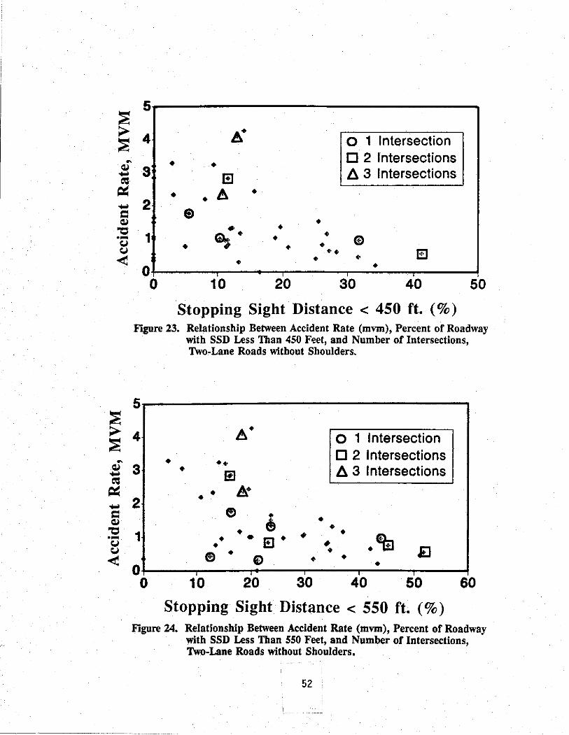
~ 5

> 4 A• ~ ~ • •

o 1 Intersection 0 2 Intersections /l. 3 Intersections a.I .....

= " ..... = a.I

-= ... CJ CJ

<

~ > ~ ~

a.I ..... = " ..... = a.I

-= ... CJ CJ

<

3

• 2

1

0 0

8 A • •

E>

• • ~·

• 10

• • ..

20

•

• • • ... • •

30 40

Stopping Sight Distance < 450 ft. ( % )

50

F'igure 2.3. Relationship Between Accident Rate (mvm), Percent of Roadway with SSD Less Than 450 Feet, and Number of Intersections, Two-Lane Roads without Shoulders.

5

4 A• o 1 Intersection 0 2 Intersections • •• 3 • m /l. 3 Intersections

• • A• 2 e • • e • 1 • • • ES • • l!I • • • iJ • • • e €) • • • 0 0 10 20 30 40 50 60

Stopping Sight Distance < 550 ft. (%) Figure 24. Relationship Between Accident Rate (mvm), Percent of Roadway

with SSD Less Than 550 Feet, and Number of Intersections, Two-Lane Roads without Shoulders.

52

w ...J 4 :!E cc w 3 CL.

~ z 2 w c 0 1 0 <(

.. .. .. •

.. .. ..

.. .. , .. ..

I O Control-Section!

.. ..

© & 0 G) ..

© © ... ...

O+-......-......-......--.-......-......-+--.-......-......-......-......-......-......-......-......-...,..........-......-........ -" # ©

0 10 20 30 40

STOPPING SIGHT DISTANCE < 450 FT (O/o)

Figure 25. Study Sites (1\vo-Lane Roads without Shoulders) Located on Control-Section.

53 •

50

All the analyses for the dependent variable logarithm of accidents per mile were repeated, omitting all sites on this particular control section. Many effects were no longer significant, which may be partly attributed to the reduction in the size of the data set. Table 20 contains the coefficients and their significance levels for the adopted models for the three criteria. The results in Table 20 can be compared to these modified analyses. For the 325-foot criterion, the curve-influenced intersections became insignificant (p = 0.12), leaving only the types of major intersections and AADT in the model. In the analysis of the 450-foot standard, the negative re 1 at i onshi p between accident rate and percent limited stopping sight distance was dropped from the model, leaving only the positive relationship with curve-influenced intersections. The model for the 550-foot stopping sight di stance criterion

·remained unchanged, although the significance level of the percent 1 imited distances was reduced (p = 0.04).

Another method of adjusting for differences that are known to exist among roadways, but for which we have no quantifiable measurements, was used. A constant term was introduced into the model for each different roadway, distinguished by its control number. This method allowed an individual constant adjustment of the accident rate for each different roadway. Again, some effects disappeared after incorporating this adjustment. The positive influence of intersecting roads within the influence of sight-restricted curves based on the 325-foot criterion, however, increased in its effect. The coefficient increased to 0.41, compared to 0.36 previously, with a significance probability of 0.01. All effects related to stopping sight distance (the relative amounts and number of intersections) were no longer significant (p > 0.05) in the analyses of the 450-and 550-foot standards.

These results are more meaningful when compared to similar analyses of the previous data set. For comparison, two-lane roads with shoulders were subjected to the same adjustment of the accident rate for different roadways. In the analysis of the two-lane roads with shoulders data set, no changes in the models resulted. The models remained remarkably consistent in terms of the sizes of the coefficients as well. The limited data available for the analysis of two­lane roads without shoulders cause the ambiguous results to be open to question. The consistency of the analytical results of the larger sample of two-lane roads with shoulders can be interpreted with more confidence.

Four-Lane Divided Roadways. An attempt was made to study four-1 ane divided roadways in the hope of identifying matched pairs for analysis. The extreme variability in the data could be better controlled by creating paired observations for analysis. The requirement, of course, was that one segment of each pair contained limited sight distance curves, while the other did not. The creation of 41 matched segment pairs yielded only a dozen pairs that satisfied that requirement. Thus, the 1 imited data did not allow the more promising analysis; however, the data obtained are in included in Appendix A.

Five-Lane Roadways. Insufficient road sect ions were i dent i fi ed by the highway districts to allow consideration of these types of roads. Only 12 miles of curbed roadway and 36 miles of uncurbed 5-lane roads were identified as potential study sites.

54

Summary

Two 1 arge data bases consisting of 222 one-mile 1 ong study segments representing nearly 1500 accidents were assembled to evaluate the effects that available stopping sight distance along crest vertical curves have on accident rates. The study sites were carefully screened to control for other geometric and operational conditions that could affect accident rates. All study segments were two-lane roadways with 55 mph posted speeds and were located in rural areas of east and central Texas. The study segments with sight distance limitations generally had modest deficiencies; that is, sight distance was generally worse than the AASHTO minimum requirements for a 55 mile per hour design, but better than the AASHTO minimum requirements for a 45 mile per hour design.

The following are the most significant findings:

1. The relationship between K factors and/or available sight distance on crest vertical curves on two- lane roadways and accidents is difficult to quantify even when a large data base exists.

2. The AASHTO stopping sight distance design model alone is not a good i ndi ca tor of accident rates on two-1 ane rura 1 roadways in Texas. Thus, adherence to the model alone in designing vertical curves on reconstruction projects may not result in cost-effective projects.

3. Where there are intersections within the 1 imited sight distance portions of crest vertical curves, there is a marked increase in accident rates. It should be noted, however, that this finding may not hold true outside of the AADT ranges investigated in this sutdy (1500 to 6000 vehicles per day).

4. It can be inferred that other geometric conditions within limited sight distance portions of crest vertical curves could also cause a marked increase in accident rates. An example would be a sharp horizontal curve hidden by a crest vertical curve.

55

IV. OPERATIONAL EFFECTS OF LIMITED SIGHT DISTANCE

The objective of the operational studies were to determine whether or not limited sight distance on crest vertical curves has any significant operational effect on driver behavior. To satisfy this objective, a literature review and several field studies were performed. The literature review was designed to provide basic information on previous studies conducted for similar purposes. This review also provided direction for the study design in the operational analysis.

Field study sites were selected based on considerations developed from the literature review and overall objectives of the study. The field studies were conducted to gather data concerning driver performance on crest vertical curves that provide less than the AASHTO (l) minimum sight distance required by the overall design speed of the roadway. Statistical analyses were performed on the data collected so that conclusions could be drawn from the information collected in the field. The following discussion presents the results from these activities.

Past Research

A brief literature review was performed to identify previous research pertinent to this study. A study by Mclean (33) found that limited sight distance crest vertical curves on two-lane roadways in Australia have very little effect on vehicle speeds. A study by Pol us, et. al. (34), however, found that limitations in sight distance on two-lane roadways in Israel did appear to cause vehicles to reduce their speed. Polus developed several models to describe the effect of various geometric features on the speeds of the vehicles being studied. One of the dependent variables given in this analysis dealt with vertical curvature and is shown to have some reduction effect on vehicle speeds. Further research by Messer (32), done in the United States, indicated that speed differentials of 10 miles per hour or greater between passenger cars and trucks on limited sight distance curves may cause safety and operational problems.

The literature review suggested that there is no overall consensus as to what effect limitations in crest vertical curve sight distance have on driver behavior. This conclusion was not surprising, given the difficulty of isolating the driver performance effects of sight distance limitations in a field study environment. If, as some of the research indicates, sight distance limitations do influence driver behavior, the question then becomes whether or not these effects are significant enough to effect operations and/or safety. The aim of this section of the report is to provide some additional insight into the operational aspects of limited sight distance on crest vertical curves.

56

Study Design

The study design used in this analysis involved two basic steps. The first step was to define some criteria and develop a methodology by which field study sites could be identified. The second step was to develop a methodology for collecting the necessary vehicle performance data.

Site Selection Criteria. It was determined that two-lane rural highways offer the best opportunity for detecting vehicle speed changes caused by limited sight distance. Two-lane rural highways provide the restrictive geometry and the volumes necessary to limit the options a driver has in reacting to differing roadway conditions. On roadways with a high volume and continuous alignment changes, drivers will generally avoid encroaching (i.e., riding the centerline) into an opposing lane because of the frequency of oncoming traffic. It has been determined, however, that five to six percent of Texas drivers (J.l) will use shoulders as an additional area for maneuvering during regular operation. Paved shoulders provide the driver with more room to maneuver and thus may cause a change (depending on shoulder width) in the way that the drivers react to perceived geometric limitations. Roadways both with and without shoulders were considered in order to provide a broader basis for analysis and to increase the number of potential study sites. The type of vertical curve was also considered in the selection process. AASHTO defines two different types of vertical curves for classification purposes as shown in Figure 26 (l). Since the type of curve involved may have an effect of its own, it was considered desirable to study curves of each type. Each potential section of roadway was evaluated for the following criteria:

I. The section must contain curves with less than the AASHTO required minimum stopping sight distance for a design speed of 55 miles per hour;

2. The section must be in a rural area;

3. The pavement cross section must be consistent throughout the section;

4. There must be no intersections on the section that require vehicles on the roadway being studied to stop; and

5. Adjacent land use should be similar throughout the section.

It was determined that Districts IO, II, and I9 located in the Tyler/Nacogdoches area of East Texas provided the best opportunity for finding good study sites. This 33-county region of the state has older highways and rolling terrain which are most likely to contain vertical curves with available stopping sight distance less than current AASHTO requirements for a 55 mile per hour design speed. These districts also contain an extensive network of two-lane rural highways from which study sections could be chosen.

57

VPI

VPT

TYPE I

VPT

TYPE II

VPC: VP!: VPT:

Gi ,Gz: A: L:

VPC

Vertical Point of Curvature Vertical Point of Intersection Vertical Point of Tangency Tangent Grades in Percent Algebraic Difference Length of Vertical Curve

~Pl ~

~A

VPT

Figure 26. ·Types of AASIITO Crest Vertical Curves.

58 i

Each of the districts that was contacted provided the information used in making the se 1 ect ion of study sections. Pl an and profile sheets, a 1 ong with roadway inventory logs for all sections of two-lane roadways containing limited sight distance vertical curves, were obtained for analysis. The information gained from this material included horizontal and vertical curve locations and design information, locations for intersecting roadways and drainage structures, and some pavement cross-section information. This information, along with video tapes and computer listings of the vertical geometry for each section, was used to select the study sections.

The first step in the selection process involved locating control sections containing vertical curves with available sight distance less than 450 feet (AASHTO minimum sight distance for a 55 mile per hour design}. This step also involved selecting limited sight distance curves that could be paired with a control curve (either a tangent section or a curved section with AASHTO minimum sight distance} within the same control-section of roadway. A paired analysis was considered the most appropriate way of handling the speed change data. The curves on each section were studied simultaneously in order to monitor the same drivers as they pass over each curve. By tracking individual drivers at each curve, a more accurate assessment of changes in driver behavior could be made.

The next step in the site selection process was to control, as much as possible, for the various other factors that might effect driver behavior. These factors, as indicated previously, include the presence of intersecting roadways, type of adjacent land use, proximity to population centers, and similar roadway cross-sections. Similar grades for control and 1 imited sight distance curves and grades of less than four percent were also considered desirable. Controlling for the previous two factors provided the opportunity to eliminate the possible effect of grade.

A final consideration used in the selection process was the relative isolation of potential study curves from other geometric features. Messer's procedure (32} was used to evaluate the relative isolation of the study curves from other geometric features. This procedure states that a geometric feature should be at least 1500 feet from any other geometric feature in order for it to be considered isolated. Isolation, in this case, means that the feature will be the only geometric factor influencing driver behavior at a given point in the roadway. I sol at ion was considered necessary to maximize the possibility of detecting vehicle operational changes caused by various degrees of sight distance limitations.

Data Collection. The data collection strategy required for this study focused on defining and collecting vehicle performance information that was most 1 ikely to produce meaningful results. As a first step operational criteria were developed in order to establish whether or not there was any noticeable effect on driver behavior. For this study, an operational effect occurred when driver behavior was altered in response to a perception that the sight distance was not sufficient for the speed at which the vehicle was traveling (i.e., the driver slows down}.

59

The primary measure of effectiveness used to determine whether or not there was a significant effect on driver behavior was speed differential between the control and limited SSD curves. Review of current research (32) and the 1985 HCM methodology (35) indicated that speed differentials greater than 10 miles per hour (especially between trucks and passenger cars) can cause significant operational and safety problems. Current research (36) also indicates that four miles per hour is the minimum practical measurement for a speed differential: in other words, speed differentials less than four miles per hour are within the limits of normal driving behavior and/or the accuracy of the speed measurement process. In order to eliminate the possible effect of slower vehicles on the speeds of faster vehicles, only vehicles traveling under free flow conditions were studied. Vehicles were defined as operating under free flow conditions if their headways were greater than five seconds (35). For this reason, it was also necessary to collect headway data. The most effective method of collecting the speed and headway data required for each site was the Texas Transportation Institute's (TTI) automatic data collection system, which consists of three basic parts:

1. Tapeswitch sensors; 2. A Golden River Environmental Computer (EC); and 3. A Zenith 171 portable laptop computer.

The tapeswitch sensors are composed of two elongated strips of metal separated by an air gap and covered by a heavy-gauge plastic coating. When a vehicle hits a tapeswitch, the metal strips are pressed together creating a voltage change between the EC and the switch. These sensors were placed in the roadway perpendicular to the travel path(s) of the vehicles being studied and then connected to the environmental computer.

The EC is a type of microcomputer used for signal conditioning. The EC continuously scans its 24 input "lines" (organized into three "ports" of eight lines each) at 1/600th second intervals. When a tapeswitch voltage drop was received on one of the 1 ines connected to the EC, a 12-character "word" labeling the activation was produced. This "word" contained four characters to denote the port and line number of the activation and eight characters to represent the time it was received. The time was read from the EC's internal clock in a hexadecimal format.

A Zenith 171 was used to store the "words" produced by the EC. This storage was accomplished through the use of several communications programs that allowed the EC and the Zenith to "talk" to each other. The program used to read the data sent from the EC, displays the port and line number of each signal on the screen of the Zenith as it is received. This feature was used to monitor the operation of the system so· that any malfunction could be quickly identified and corrected. The signal information was stored in the memory buffer of the Zenith until it was full, at which time the data were copied to a floppy disk for permanent storage.

Setting up this system involved installing the tapeswitches at the desired locations, connecting them to the EC, and connecting the EC to the Zenith portable computer. The tapeswitches were secured to the roadway using four-inch wide strips of an adhesive matting material. After all of the sensors were

60

placed in the roadway, connections were made to the EC using multiconductor cable laid along the sides of the roadway. When all of the connections were made, each sensor was assigned to a line on the EC that would monitor the sensor switch. The Zenith portable was then connected to the EC using a serial line.

For each of the curves under study, tapeswitches were set up in pairs in both directions of travel at three positions along each of the curves (see Figure 27). For this particular study, the tapeswitch pairs had a 10-foot separation in order to create a speed trap for collecting the necessary speed and headway data. The 10-foot separation was selected as the best compromise between minimizing the effect of deceleration between the detectors and maximizing the accuracy of the speed measurement.

In cases where a suitable control curve was not located close enough to a 11 ow a comparative study, a level tangent section was subst i t.uted as an alternative. This substitution still allowed for a comparison of speeds between control and limited sight distance conditions. Tangent controls were set up with two pairs of tapeswitches 500 feet apart on a level grade prior to the start of the limited sight distance curve. Each pair of tapeswitches is called a station and can be considered a point along the curve. Data were collected at each site so that any changes in vehicle speed, for both passenger cars and trucks under both day and night lighting conditions, could be detected.

The data collection system was set up in both directions of travel to maximize the amount of data collected. The daytime data collection occurred during the late afternoon just before sundown, and the night data collection was conducted around midnight. This approach allowed for an analysis of driver behavior under different lighting conditions. The night data provided the most restricted visual conditions and should have produced the most noticeable difference in behavior. Each study period was approximately four hours long.

61

"' "'

v ,/

- ~-

Station 1

I~

T "\ h P . (1 O' S apesw1 c air r l epara ion

---@-~ Multiconductor Wire

Station 2

CONTROL

500' . I

-~

-~

Station 3 Station 4 Station 5

Limited Sight

Distance

Figure 27. Typical Study Site Set-Up Using a Tangent Section as the Control.

Study Sites

Three study sections were selected for the data collection effort. The study sections were along US Highway 59 (US 59), US Highway 175 (US 175), and US Highway 80 (US 80). The study sections on US 59 and US 175 had heavy truck volumes during both day and night conditions. The truck volumes on US 80 were considerably lower due to its proximity to Interstate 20. Table 20 gives a brief summary of the characteristics of the study curves within the study sections.

TABLE 20. Characteristics of Crest Vertical Curves Selected as Field Study Sites.

Study Limited K Sight Control K Sight Site Curves Distance Curve Distance

us 59 Type I 107 372 Tangent us 175 Type I 93 351 Type I I 177 493 us 80 Type II Tangent

Once the desired control sections were located, it was necessary to find potential study sites within these sections. As mentioned previously, independent curves were desired in order to minimize the influence of any other geometric feature. Unfortunately, given the topography in the study areas and the relatively small number of limited sight distance curves available, it was not possible to select a totally isolated curve for each site. Similar shoulder types and grade changes were also sought in the curve selection process; however, because consistent curve designs are often used throughout a short section of highway, controlling for grades between curves with different lengths was not always possible.

US 59 Study Site. The cross section of the US 59 study site was a two-lane undivided roadway with full width paved shoulders. The limited sight distance curve for this site is also the only curve in the section without climbing lanes. For data collection purposes, the study site consisted of a single Type I vertical curve (minimum sight distance= 372 ft.) and a tangent section for the control site. The data collection system was set up with two stations on the tangent section and three stations on the limited sight distance curve. A sixth station was set up to the north of the limited sight distance curve at the base of a 1900 foot grade. All stations were set up for both directions of traffic. Figure 28 shows the configuration of the site as it looked during the data collection. An unexpected equipment failure at this site allowed only four stations in each direction to be monitored and only during night conditions. The operative and inoperative stations are also shown in Figure 28.

63

L'' I I I c~ I

Station 1 Station 2 Station 3

X Station not operative.

. I D I I

Stat'1on 4 Station 5

Limited Sight

Distance

Figure 28. US 59 Study Site Set-Up.

I 1: ~

Station 6

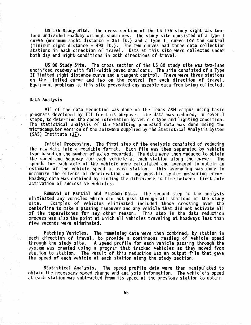
US 175 Study Site. The cross section of the US 175 study sight was two-1 ane undivided roadway without shoulders. The study site consisted of a Type I curve (minimum sight distance = 351 ft.) and a Type II curve for the control (minimum sight distance = 493 ft.). The two curves had three data collection stations in each direction of travel. Data at this site were collected under both day and night conditions in both directions of travel.

US 80 Study Site. The cross section of the US 80 study site was two-lane undivided roadway with full-width paved shoulders. The site consisted of a Type II limited sight distance curve and a tangent control. There were three stations on the limited curve and two on the control for each direction of travel. Equipment problems at this site prevented any useable data from being collected.

Data Analysis

All of the data reduction was done on the Texas A&M campus using basic programs developed by TTI for this purpose. The data was reduced, in several steps, to determine the speed information by vehicle type and lighting condition. The statistical analysis of the resulting processed data was done using the microcomputer version of the software supplied by the Statistical Analysis System (SAS) Institute (37).

Initial Processing. The first step of the analysis consisted of reducing the raw data into a readable format. Each file was then separated by vehicle type based on the number of axles recorded. The data were then reduced to obtain the speed and headway for each vehicle at each station along the curve. The speeds for each axle of the vehicle were calculated and averaged to obtain an estimate of the vehicle speed at each station. This averaging was done to minimize the effects of deceleration and any possible system measuring error. Headway data was obtained by finding the difference in time between first axle activation of successive vehicles.

Removal of Partial and Platoon Data. The second step in the analysis eliminated any vehicles which did not pass through all stations at the study site. Examples of vehicles eliminated included those crossing over the centerline to make a passing maneuver and any vehicle that did not activate all of the tapeswitches for any other reason. This step in the data reduction process was also the point at which all vehicles traveling at headways less than five seconds were eliminated.

Matching Vehicles. The remaining data were then combined, by station in each direction of travel, to provide a continuous reading of vehicle speed through the study site. A speed profile for each vehicle passing through the system was created using a program that tracked vehicles as they moved from station to station. The result of this reduction was an output file that gave the speed of each vehicle at each station along the study section.

Statistical Analysis. The speed profile data were then manipulated to obtain the necessary speed change and analysis information. The vehicle's speed at each station was subtracted from its speed at the previous station to obtain

65

the speed differentials between each pair of stations. Since the same vehicle was used to find the speed differential at each pair of stations, the data are considered to be paired and the appropriate statistical test is a paired t-test (38).

The first step in the statistical analysis was to perform sample size calculations to insure that there was an adequate number of observations in each class breakdown. The class breakdowns were defined by site, direction, lighting condition, and vehicle type. Vehicle types were defined as either two axle or more than two axle (i.e., passenger cars and trucks). The speed differentials were first analyzed to determine their frequency distribution by site, direction, lighting condition, and vehicle type.

The next step in the analysis was to determine the frequency distribution of the speed differentials to get an overall idea of how vehicles were reacting to the changes in alignment within the study site. To determine the significance of the speed differentials, paired t-tests were conducted on the sample means. The data were assumed to be approximately normally distributed, and because a minimum headway of five seconds was required, the sample speed differentials are independent. The research hypothesis under investigation in this study was that there was no difference between the mean for the speed differential between the control and the limited sight distance curve (i.e., the mean difference is equal to zero). The alternative hypothesis, then, was that the mean difference was significantly different than zero.

A practically significant difference in vehicle speeds, between the control and the limited sight distance curves, was taken as four or more miles per hour (36) for this analysis. Even if statistically significant, speed differentials of less than four miles per hour were not large enough to be meaningful from a practical point of view. A four-mile-per-hour threshold also eliminated the effect of any measuring error within the data collection system. Any means that were numerically greater than four were also tested to see if they were statistically greater than four. The null hypothesis for this analysis, therefore, was that the mean speed differential was statistically greater than four.

Results

The results of this ope rat ion a 1 analysis are primarily concerned with determining whether or not there was any change in vehicle speeds due to differences in available sight distance on the curves under study. A discussion of the results of the frequency distribution analysis follows and is accompanied by frequency di stri but ion p 1 ots comparing differences by direction, 1 ighti ng conditions, and vehicle type. The results of the paired t-test analysis are also given by site, direction, lighting conditions, and vehicle type.

Frequency Distributions. The frequency information was summarized using three mile per hour class intervals centered on a difference of zero. Class interval grouping provides a smoother, more normal distribution which is not only easier to visualize, but also easier to analyze. All distribution plots are given in percent frequency to account for the, variation in sample sizes. The

66

information from the two sites is given separately, due to the wide variation in site conditions and amount of data collected. The frequency information for US 175 is given for the speed differential between the two study curves. Westbound vehicles were traveling from the control toward the limited sight distance curve. Eastbound vehicles, on the other hand, were traveling away from the limited sight distance curve. The data for US 59 is given for each speed differential in the northbound direction. The northbound direction on US 59 gives vehicles traveling from the control to the limited sight distance curve.

Figure 29 shows a comparison of day and night conditions for passenger cars and trucks for each direction of the US 175 study site. The distributions for all cases appear to be approximately normal. The day and night distributions for the westbound direction are shifted a substantial distance below zero, but appear to be the same for both cars and trucks. This shift below zero may be the result of a driver reaction to a perceived limitation in sight distance. The speed variation in the eastbound direction, however, shows a much flatter and broader distribution of speeds during the day. The distribution for the daytime data is also more nearly centered around zero. This difference means that, at night, the drivers were showing a greater positive deviation in speeds (e.g., they were more inclined to speed up between the limited sight di stance curve and the control curve). The drivers are moving onto a section of roadway with adequate sight distance and maybe, as a result, are speeding up.

A comparison of cars and trucks by lighting condition and direction is given in Figure 30. The distributions here are also approximately normal. The distribution for the westbound direction shows that cars and trucks tend to slow down as they approach the limited sight distance curve. The magnitude of the reduction is greater for trucks, although the relative difference appears to be the same for both day and night conditions. The eastbound direction shows a positive speed differential during both day and night. In addition to this difference, there is a more pronounced speed increase for trucks than cars at night in the eastbound direction. It is not clear why the drivers show more consistent speed changes at night.

The final comparison for the US 175 site is given in Figure 31. These distributions compare directions of travel by vehicle type and lighting condition. The difference in speed differentials for vehicles approaching and moving away from the limited sight distance curve is quite obvious in these comparisons. In every case the speed differentials are shifted into the negative region for vehicles approaching the limited sight distance curve, whereas the speed differentials are positive for vehicles moving away from the limited sight distance curve. The distributions also show a greater difference in the reaction of truck drivers between directions. This differential is not related to the downgrade on the departure from the limited sight distance because the speed increase is too large. These distributions provide support for the existence of operational effects related to available sight distance on crest vertical curves.

67

·12 -·

·m o:> 80

&O

-:::-! .to

e:. ~ 30

g. e 20

"' 10

0 ·12 ·9

Day vs Night [US175W] (PC)

.. a ... 3 o 3

Speed Differential e

Day vs Night [US175E] (PC)

·8 ·3 0 3 8

Speed Differential

9

~ D•y

~ Nlghl

9

so

12 -12

12 -12

-·

·9

Day vs Night [US l 75W] (T)

-6 ·3 0 3

Speed Differential

Day vs Night [US175E] (T)

-6 -3 0 3

Speed Differential

Figure 29. US 175 Frequency Distribution Plots for Day vs Night.

8

6

&ml D•w ~Night

9

9

12

12

60

60

~

li 40

~ i;' 30

5 " l 20

10

0 -12 -·

60

-12 -9

Cars VS Trucks [US175W] (Day)

-· -3 0 3 • Speed Differential

Cars vs Trucks [US175E] (Day)

-e .. 3 o a Speed Differential

6

~ c.,. ~ Trucks

9

m C•r•

~Truck•

9

12

12

60

60

-:::-5 40 g " e:. "' 30 !l " g' 20 it

10

60

60

'? 40 " 0

~ i;' 30

" ~ "' 20 " it

10

0

-12 -·

-12 -9

Cars vs Trucks [US175W] (Night)

-6 -3 0 3

Speed Differential 6

Cars vs Trucks [US175EJ {Night)

-· -3 0 3 6 Speed Differential

Figure 30. US 175 Frequency Distribution Plots for Cars vs Trucks.

~Cara

~ Trucks

9

9

12

12

60

60

-::-" 40 " " ~ "' 30

l 20 " Lt

10

0 -12 -9

...., 0 60

60

i? ~ •o

&! ~

~ 30

" " ~ [ 20

10

0 -12 -9

..

East vs West [US 1750] (PC)

-· -3 0 3 6 9 12 Speed Differential

East vs West [US175D] (T)

Im:! We•t

~ E••t

-· -3 0 3 6 9 12 Speed Differential

60

10

-12

60

60

i? " 40 g

~ "' 30 " " " ~ O'

" Lt 20

10

0 -12

-9

-9

East vs West [US175N] (PC)

-6 ·3 0 3 Speed Differential

East vs West [US175N] (T)

-6 -3 0 3 Speed Differential

6

6

.figure 31. US 175 Frequency Distribution Plots for East vs West

m w ••• ~ E•••

9

m Weil

~ Ea1t

9

12

12

The speed distributions for the US 59 site are given in Figure 32. These distributions show the speed differentials between each pair of stations in the northbound direction for cars and trucks during night conditions. The differences between car and truck speed differential distributions are very small over the entire study section. There is, however, a rather large decrease in speeds as the vehicles approach the limited sight distance curve. These data were only collected at night, so the vehicles were operating under the most restricted sight distance conditions and thus may be showing a greater reaction to the limitation in sight distance. The speed decrease for trucks in this situation could be explained by the grade. The almost identical reaction of the passenger cars over the same section of roadway, however, does not support this explanation; i.e., if grade were the cause of the speed differential, passenger cars would not be expected to show the same speed reduction as trucks.

Paired Analysis. The results of the paired analysis are also summarized in several figures for each site and direction. Each figure contains the vertical geometry data for the study site, the location of the data collection stations, and a table summarizing the mean speed differentials for each class of data collected at that site. Each figure is drawn to the scale indicated on the drawing.

Figure 33 shows the data for the eastbound direction of the US 175 study site. There is a small decrease in speed (delta 1) for vehicles approaching the 1 imited sight distance curve. Figure 34 shows the data for the westbound direction of travel. There is also a decrease in speeds (deltas 3 and 4) for vehicles approaching the limited sight distance curve from this direction. These decreases in speed were found to be statistically different from the hypothesized mean of zero for both directions of travel. The speed differential for eastbound delta 1 and westbound delta 4 were not, however, large enough to be of practical significance (i.e., greater than four miles per hour).

The westbound speed differential for delta 3 was both practically and statistically significant, with values ranging from minus five to minus eight miles per hour. The distance between these two stations is such that it is difficult to tell exactly where the actual decrease in speed occurred, but it is possible that this speed reduction is the result of drivers reacting to the limitation in sight distance before they actually enter the curve. In contrast, there was no speed decrease measured for vehicles traveling westbound on the control curve. There was a statistically significant increase in speeds, but again it was not large enough to be of any practical significance. Vehicles traveling eastbound on the control curve did exhibit a statistically, but not practically significant, decrease in speed.

For the most part the speed changes at this site were so small that it is not possible to tell whether they were caused by the grade on the curves or were driver reaction to the limited sight supported by the data. Because of the speed increases in the uphill direction of the control curve and the speed decreases in the downhill direction of the control curve, grade as the causative effect of the speed differentials did not make any sense.

71

100

90

80

ti 70

~ 80

~ &O

g 4.0

.[ 30

20

10

0 •12

Cars VS Trucks [US59N] (Night) DI Cars vs Trucks [US59N] (Night) D2

·ii ·6 ·3 0 3 6

Speed Differential

100

90

80

~ 70 u

J! 60 ~

~ 60

" 8 40 C"

J: 30

20

10

0 •12

~Car•

fZ?l Truck•

9 12

100

90

80

510 t 60

"" ~ &O ~ U •o " C" ~ 30 tl:

20

10

0 ·12 ·9

Cars VS Trucks [US59N] (Night) D3

m Carl

~ Truck1

·9 ·6 ·3 0 3 6 9 Speed Differential

-6 -3 0 3 Speed Differential

12

6

mD C•ra

~Truck•

9

Figure 32. US 59 Frequency Distribution Plots for Cars vs Trucks by Station.

12

..... w

Horizontal Scole ,im 0 100 200 .300 400

Verticol Scale 1tt • 't 1Mo ;;--:o

VPC

Ll1 250'

L\2 240'

DIRECTION OF TRAVEL (EAST)

VPC VPT

Station 3

400'V.C.

VPI .... 2."Jo::

1910'

Station 4

VPI -0.083

900'V.C. I CONTROL

450' Ll5 450'

MEAN SPEED DIFFERENTIAL LIGHTING VEHICLE SAMPLE Ll1 Ll2 Ll3 Ll4 {15

1YPE SIZE DAY CAR 233 -1.93' +0.46' +2.44* -0.46* -2.14'

TRUCK 25 -1.44' +D.60* +3.12* -0.48* -1.72* NIGHT CAR 49 -1.14* +0.82* +0.92 -1.22* -1.73*

TRUCK 22 -0.95' +0.64* +4.95*t -1.00• -2.91' *Me on speed differential not equal to zero ( a "" 0.05 ). t Mean speed differential significantly greater than four (a "" 0.05).

Figure 33. Results From the US 175 Eastbound Study Site.

700'V.C.

Horizontal Scale 1~ 0 100 200 JOO 400

Vertical Scale tZ' 4 't 10 20 JO 40

VPT VPC

'< ·Oo-?"

1::.5 250'

M 240'

DIRECTION OF TRAVEL (WEST)

VPC VPT

400'V.C.

VP! .... <.107.

1::.3 191 O'

Stolion 10

VPI -0.08%

900'V.C.

450'

I CONTROL

1::.1 450'

MEAN SPEED DIFFERENTIAL LIGHTING VEHICLE SAMPLE 1::.5 M 113 112 111

TYPE SIZE DAY CAR 161 +2.36' -1.09* -5.16*t +2.01* +1.94*

TRUCK 22 +2.86* -0.73* -8.00*t +2.14* +3.00* NIGHT CAR 29 +1.52* -1.14* -3.97* +0.69 + 1.69'

TRUCK 18 +3.00* -0.72"' -7.39*t +2.61* +2.89* •Mean speed differential not equal to zero (a - 0.05). t Mean speed differential significantly greater than four (a = 0.05).

Figure 34. Results From the US 175 Westbound Study Site.

700'V.C.

VP ' ~Oo ~

As can be seen in Figure 35 for the northbound direction of the US 59 study site, vehicle speeds increased up to station 2, at which point there is a sharp decrease to station 3 (near the crest). The frequency distributions showed the same decrease in speeds. This decrease in speed was shown to be significant in both a practical and a statistical sense. The upgrade on this vertical curve is approximately 1200 feet long at 2.94 percent. According to Chapter 8 of the "Highway Capacity Manual," a 7-mile-per-hour decrease in speed could be expected for trucks operating in the 300-pounds-per-horsepower class on such a grade.(35) This fact, however, does not explain the similar speed decrease experienced by passenger cars on the same grade. It is possible that the decrease in speed is caused, at least in part, by the limitation in sight distance.

The southbound direction of travel on US 59 (Figure 36) does not indicate any reduction of speed over the limited sight distance curve. This observation may be due to the lack of data collection stations on the uphill portion of the curve. Any existing change in speeds would not be noticeable without more data from the approach side of the limited sight distance curve. The long downgrade (1900 feet at five percent) on the approach to the limited sight distance curve in this direction may also have had an effect on the vehicle speeds. The downgrade would not, however, explain the slight speed differential experienced by vehicles traveling from station 6 to station 8. In any event, it is not possible to make a judgment as to whether or not vehicle speeds changed in response to the limitation in sight distance in the southbound direction.

Conclusions

The purpose of this study was to determine whether or not limited sight distance on crest vertical curves has any practically significant effect on vehicle speeds. Examination of the data for both sites does not appear to indicate any significant difference between day and night operations, except for the frequency distribution data for US 175 on eastbound trucks, which seemed to indicate some difference in operations. This difference does not appear to be of any significance due to the small difference in mean speed differentials. There also appears to be no significant difference between the speed differentials for trucks and those for passenger cars, except for two cases on US 175. In the westbound case (between stations 10 and 9), there is a slightly greater decrease in speed for trucks during both day and night conditions. Conversely, the eastbound trucks between the same stations show a greater increase in speed during both day and night conditions. Again these differences are not large enough to be of practical importance.

75

Horizontal Scale 100 0 100 200 300 400

Vertical Scale 10 0 10 20 30 40

Station 1

I Bridge ( 150')

VPC

..... "'

DIRECTION OF TRAVEL (NORTH)

VPI ?-943

Station 3 .\- . Station 4

Station 2 700'V.C.

LIMITED SIGHT

DISTANCE 400'V.C.

VPI

L'l 1 L'l2 63 1200' 500' 300'

MEAN SPEED DIFFERENTIAL LIGHTING VEHICLE

TYPE NIGHT CAR

TRUCK

SAMPLE SIZE 87 24

+6.62*1 +9.04*1

-5.59*1 -5.25*1

* Mean speed differential not equal to zero (a = 0.05). 1 Mean speed differential significantly greater than four (a = 0.05).

-0.53* -0.96*

Figure 35. Results From the US 59 Northbound Study Site.

Bridge (75') '.J . .:>a-%"

Horizontal Scale 100 0 100 200 300 400

Vertical Scale 10 0 10 20 30 40

Station 10

VPC

..... Bridge (150')

.....

DIRECTION OF TRAVEL (SOUTH)

Station 8

Station 9 700'V.C.

limited Sight

Distance

VPI

63 62 61 700' 500' 1300'

MEAN SPEED DIFFERENTIAL LIGHTING VEHICLE

TYPE SAMPLE

SIZE t::,3 62 61

NIGHT CAR TRUCK

67 24

+4.66*! +6.17*1

+2.42* + 1 .96*

* Mean speed differential not equal to zero ( e< = 0.05). t Mean speed differential significantly greater than four ( C< = 0.05).

-0.36 -1 .42*

Figure 36. Results From the US 59 Southbound Study Site.

VPI

V. COST EVALUATION OF VERTICAL SIGHT DISTANCE IMPROVEMENTS

The cost of improving a roadway's existing vertical alignments consists of three components, construction, operation, and accident costs. These three cost components should be identified and considered to quantify the effects of such improvements on a roadway's vertical alignment.

This chapter provides a methodology to estimate those costs involved with improving a roadway's vertical alignment. This methodology consists of four basic components:

I. Development of typical cross sections for various roadway types; 2. Identification of cost values; 3. Development of costs relationships; and 4. A cost analysis.

Development of Typical Cross Sections

Prior to identifying costs or developing costs analysis, typical cross sections for the five different roadway types were developed:

I. Two-lane without shoulders; 2. Two-lane with shoulders; 3. Four-lane divided; 4. Five-lane with shoulders; and 5. Five-lane with curbs and gutters.

The Federal Highway Administration (FHWA) requires that the design speed of the entire roadway meets current state standards for the posted speed limit on facilities. For example, if the design speed is 55 miles per hour, the stopping sight distance must be set at 55 miles per hour. Design standards in the State Department of Highways and Public Transportation (SDHPT} Highway Design Division Operations and Procedures Manual (39) were used to develop typical cross sections for study roadway types. These standards are consistent with current AASHTO policy (1) and were used to establish vertical alignment criteria for the desired operating speed of 55 miles per hour on study roadways.

Design factors assumed in this analysis include cross slopes, median widths, shoulder widths, etc. and either meet or exceed the state's minimum design standards. Right-of-way requirements included in these figures are general estimations with specific consideration given to the 30-foot "cl ear zone" from the outer edge of the pavement. The fore and back slopes of ditches, 6:1 and 3:1 respectively, are design variables held constant for this analysis. A minimum depth of two feet was assumed for the ditch through a crest curve section. Table 21 is a summary of the cross-section design variables used for this study.

78

TABLE 21. Assumed Cross-Section Design Variables for Analysis.

SlooesC3) Pavement<1> Stabi l i zed<1> ROW(2) Depth. In. Base Depth, Width,

Ditch Roadway Shoulder Fore Back Lane 1 lane 2

In. Ft.

2 Lane w/o shldr. 1 8 120 6:1 3:1 2 lane w/shldr .. 2 12 120 6: 1 3: 1 4 lane divided 3 14 300 6:1 3:1 5 Lane w/shldr. 3 14 220 6:1 3:1 5 Lane C&G 3 14 220 6:1 3:1

TTI average values on statewide research project. Accepted minimum values.

2.0% 2.0% 2.0% 2% 1.8% 2% 1.8% 2%

Source: (1) (2) (3) Source: SDHPT • Operations and Procedures Manual, suggested values ..

3.0% 3.0% 3.0% 3.0% 3.0%

Median<3l llidth Slope

Ft.

76 8.0% 14 1.5% 14 1.5%

Another cross-sectional element that varies from project to project is the thickness of pavement and treated subgrade. Pavement thickness is primarily a function of the functional class of the roadway, i.e. traffic volume and traffic composition, and ranges between one and three inches in depth. Stabilized base depth, like pavement thickness, is dependent on traffic volumes and composition with values ranging between 8 and 14 inches. The values shown for pavement and stabilized base depths in Table 21 are the result of a statewide survey conducted by the Texas Transportation Institute. While existing site factors and possibly preferred design practices may dictate depths different from Table 21 values, these values serve the purpose of this study. Costs developed from these values, discussed in a later section, may be modified to represent regional or site specific requirements.

Identification of Cost Values

As previously mentioned, the costs associated with improving the vertical realignment of an existing facility include:

1. Construction costs, 2. Operation costs, and 3. Accident costs.

The estimates of realignment costs presented in the remainder of this chapter include only the first two components: construction and operation costs.

Construction Costs. The first component cost evaluated was construction costs. These costs include right-of-way acquisition, earthwork, pavement, stabilized base, detour construction, and other extra construction items required to reconstruct the roadway to meet current SDHPT design criteria (39). For the purpose of this study, cost values for each item represent statewide average prices for items of work. These prices were obtained from SDHPT Average Low Bid Unit Prices By District (45). Because the example costs presented in this study are based on statewide average low bid prices, they may not reflect the actual

79

unit price for work items in a particular district. For this reason, a district should draw on its own data base so the cost of such a project may be appropriately estimated for a specific area.

Construction work components related to the K factor and the resulting length of vertical curve include:

I. Right-of-way acquisition; 2. Roadway excavation; 3. Cubic yards (CY) of pavement; 4. Square yards (SY) of stabilized base; 5. Tons of asphaltic concrete base; and 6. Tons of level-up, and detour construction related items.

Additional right-of-way may be required to satisfy "clear zone," 30-foot, criteria when the vertical alignment is modified. Detour construction may also require that additional right-of-way be obtained and could in some cases be a temporary easement which is free of charge. Should this additional right-of-way have to be purchased, it should be included in the project estimate. Again, this cost must be evaluated on a project by project basis due to the high degree of variability in both policy and methods utilized by an individual district. Normally, the SDHPT retains an appraisal firm to appraise the entire tract to determine its market value. The appraised value is a function of local property values, tract size, and improvements, if any. These factors, as expected, vary from tract to tract. Information provided by districts participating in this study indicated that an average cost of rural right-of-way is approximately $3,000 per acre. This value was used for the purpose of this study.

Increasing the K factor of a crest vertical curve effectively lowers the existing centerline elevations and lengthens the curve, thus requiring earthwork, i.e. roadway excavation, to achieve the desired alignment. For the purpose of this study, only items of work considered to be additional to an existing reconstruction project were included in construction cost estimates attributable to vertical realignment.

Operation Costs. Component costs in this category include:

I. Detour maintenance; 2. Delay; and 3. Traffic handling.

These costs represent items of work, increasing project bid price, and quantifying costs to the motoring public having to use the facility during vertical realignment.

Detour maintenance costs are comprised of activities which must be performed to sustain traffic. The detour cross section, generally, does not conform to permanent pavement design standards. Therefore, it is probable that detour facilities will require resurfacing or some form of surface repair during the course of the project. While these work items may not and in most cases are not bid i terns, contractors wi 11 adjust their bid price to account for this additional work.

80

The additional construction activities required by vertical realignment will also result in additional delay costs. This cost is the result of slower travel speed and reduced lane capacity. In this report, delays were associated with three factors:

1. Annual average daily traffic (AADT); 2. Type of roadway, i.e. two-lane, four-lane divided, etc.; and 3. Reduction of capacity due to construction.

The delay resulting from slower travel speeds is a function of detour length and the difference between posted speeds before and during construction. For this study it was assumed that neither a reduced speed nor a detour because of vertical realignment, were required by the original scope of project work.

Reduced speed and detours require specialized traffic handling. While the extent of such traffic handling activities could vary greatly on a project-to­project basis, one could safely assume that additional signing and striping would be required as a minimum. Historically barricading, signing, and traffic handling are combined into a line bid item charged on a per month basis. Traffic handling during vertical realignments could affect Construction costs if the realignment is the only construction project in the area. The cost may be minimal if additional construction activities are occurring and traffic handling is already included in the project price. For the purpose of this study, it was assumed that other construction activities were present and traffic handling for the additional vertical realignment construction would not affect the project cost.

Accident Costs. Accident costs were not included in estimates of realignment costs due to a lack of data on changes in accident rates through work zones. Since the mid-1970's, studies of vehicle accident characteristics in work zones have been conducted in Texas (40), Virginia (41), Ohio (42), and North Carolina (43). These studies report only the frequency of accidents by type in highway work zones. A study by Graham, Paul sen, and Glennon ( 44) examined accident rates at 79 work zones in seven states. This study reported an average increase of 6.8 percent in accident rates during construction. There was, however, considerable variability in the changes in accident rates from project to project: 31 percent of the projects experienced a decrease in accidents, but 24 percent of the sites experienced a 50 percent or greater increase in accidents (44). The results of these studies indicate that accident rates in construction areas are a function of a variety of factors and not purely a function of the presence of construction activities. Since the available data did not permit reasonable estimates of changes in accident costs to be made, accident costs were not included in the vertical realignment cost analysis.

81

Development of Cost Relationships

In this section, identified costs are related to roadway cross-section and curve characteristics. The construction and operating costs, discussed in the previous section, can be related to either roadway cross-section or curve characteristics as illustrated in Table 22.

TABLE 22. Cost in Relation to Roadway Cross-Sectional and Curve Characteristics.

Cost Item

CONSTRUCTION

R.O.W. Acquisition

Earthwork

Pavement

Stabilized Base

Detour Construction

OPERATION

Detour Maintenance

Delay

Traffic Handling

Characteristics Roadway Curve

Width Plus 30 1 Safe Zone Length, L

Width, Back and Forth Slope on Ditches

Length,. Ldiff. inKFactor (Exist vs. 150 min)

Cubic Yard, Roadway Type Length, L

Square Yard, Roadway Type Length, L

Length, Roadway Type Length, L

Traffic Volunes, Existing Length, L

Length Construction Zone, Posted Speed, AAOT Length, L

Detour Length, Original Project Requirements Length, L

All of the cost items in Table 22, are dependent on the length of curve. This length, L, may be calculated by Equation 1.

where,

L = K * A

K = A =

curvature rate of change, 150 (current minimum). algebraic difference in grade, percent.

[1]

Curve length increases with an increase in the K factor, which increases the earthwork, pavement, stabilized base, length of detour, and possibly ROW acquisition. The two primary cross-sectional characteristics affecting costs are width and type of roadway, i.e. Farm-to-Market, U.S., or State. Each type of roadway requires a different depth of pavement and stabilized base.

Earthwork. Table 23 summarizes the effects of existing A and K factors on earthwork required to obtain an alignment conforming to a K = 150. Actual individual grades do not effect earthwork as much as the A value. Current design standards, both federal and state, suggest a maximum grade of 6 percent for the types of roadways included in this study. For this reason, a range of 0.5 to 6

82

TABLE 23. Est;mated Earthwork Quant;t;es ;n Cub;c Yards Exht;ng A and K Values to Ach;eve a K m;n = 150.

2 Lane w/o 2 Lane w/ 4 Lane Div. 5 Lanes 5 Lanes w/ A K Shoulders Shoulders W/ 76' Med. w/Shoulders C&G

75 260 320 820 550 100 100 260 320 800 540 100 125 250 310 780 530 90

2 75 620 780 1,960 1,290 305 90 600 750 1,890 1,250 280

100 590 730 1,840 1,220 270 125 540 670 1,700 1, 140 220

3 75 1,220 1,520 3,840 2,500 720 90 1, 150 1,440 3,640 2,380 650

100 1,100 1,370 3,470 2,275 605 125 960 1, 190 3,000 1,990 450

4 75 2, 100 2,630 6,610 4,250 1,460 90 1,930 2,420 6,090 3,930 1,280

100 1,810 2,260 5,700 3,690 1,160 125 1,450 1,800 4,560 2,990 790

5 75 3,480 4,350 10,830 6,920 2,680 90 3,140 3,930 9,820 6,280 2,330

100 2,880 3,600 9,040 5,800 2,060 125 2, 170 2,700 6,820 4,430 1,330

6 75 5,450 6,790 16,680 10,620 4,520 90 4,810 6,000 14,870 9,470 3,860

100 4,340 5,420 13,500 8,610 3,380 125 3,030 3,780 9,530 6, 140 2,040

7 75 8,290 10,280 24,830 15,830 7,210 90 7,200 8,950 21,880 13,930 6, 100

100 6,400 7,980 19,660 12,510 5,290 125 4,230 5,290 13,270 8,500 3,050

8 75 12,130 14,940 35,410 22,640 10,960 90 10,370 12,830 29,180 19,670 9, 167

100 9, 100 11,300 27,480 17,478 7,880 125 5,690 7, 120 17,780 11,330 4,400

9 75 17,370 21,220 49,250 31,760 16,090 90 14,640 18,010 42,580 27,230 13,330

100 12,700 15,700 37,610 23,970 11,360 125 7,600 9,500 23,540 14,970 6, 170

10 75 24,240 29,380 66,630 43, 160 22,920 90 20, 180 24,650 57,150 36,740 18,800

100 17,320 21,280 50, 140 32,000 15,900 125 9,930 12,380 30,440 19,330 8,380

11 75 33,260 39,950 88,450 57,800 31,880 90 27,370 33, 180 75,350 48, 770 25,910

100 23,270 28,400 65,720 42,270 21,760 125 12,860 15,990 38,940 24,730 11,170

12 75 48,270 53,390 115,260 76,050 43,420 90 36,500 43,910 97,580 63,650 35,000

100 30, 760 37,290 84,660 54,790 29, 180 125 16,430 20,350 49,070 31,210 14,620

83

percent grades were selected for the analysis. These grades result in an algebraic difference in grade between A= 1 and A= 12, as shown in Table 23.

To use Table 23, first identify the existing Kand A values for the crest vertical curve. Follow the row representing the existing K value to the column containing desired roadway type. This value indicates volume of earthwork in cubic yards of excavation required to achieve a vertical alignment with a K factor of 150 for an existing A value.

Pavement/Stabilized Base. These quantities are dependent on roadway type and length of curve. As previously shown in Table 21, pavement and stabilized base depths vary with roadway classification. Using the width, roadway type, and length of vertical curve, quantities for construction elements could be estimated. These estimates are shown in Table 24. By selecting the appropriate roadway type and A value, an estimated quantity for both pavement and stabilized base may be determined.

TABLE 24. Pavement/Stabilized Base Quantities Required By Existing Algebraic Difference in Grade and Roadway Type to Achieve a K Min = 150.

2 Lane w/o 2 Lane w/ 4 Lane Div. 5 Lane 5 Lane w/ A Shoulders Shoulders W/ 76' Med. w/Shoulders C&G

Pavement(1) 1 10 40 120 110 90 2 20 70 240 230 170 3 40 110 370 340 260 4 50 150 490 460 350 5 60 180 610 570 430 6 70 220 735 685 520 7 80 260 885 800 605 8 90 295 980 910 690 9 100 335 1, 100 1,025 775

10 110 370 1,220 1,140 860 11 120 410 1,345 1,255 950 12 135 445 1,470 1,370 1,035

Stabilized 1 400 670 1,470 1,370 1,030 Base<2l 2 800 1,330 2,930 2,730 2,070

3 1,200 2,000 4,400 4,100 3, 100 4 1,600 2,670 5,870 5,470 4,130 5 2,000 3,330 7,330 6,830 5, 170 6 2,400 4,000 8,800 8,200 6,200 7 2,800 4,670 10,270 9,570 7,230 8 3,200 5,330 11,730 10,930 8,270 9 3,600 6,000 13,200 12,300 9,300

10 4,000 6,670 14,670 13,670 10,330 11 4,400 7,330 16, 130 15,030 11,370 12 4,800 8,000 17,600 16,400 12,400

Notes: <1>quantity in cubic yards (CY) (2lquantity in square yards (SY)

84

Detour Construction and Maintenance. Vertical realignment of a crest vertical curve may require construction of a detour. The detour subgrade should be designed to standards similar to that of the existing or proposed pavement. This approach is suggested because the detour will be subjected to the same traffic volume and composition as normally present on the facility on a routine basis. For this reason, it was assumed that subgrade depths would vary with respect to facility type.

Depth of pavement on detours is routinely decreased due to other construction considerations. Normally, detour facility pavements consist of two inches of asphaltic concrete pavement over the suggested subgrade. Quantities for the two lane roadways are based on a 24-foot wide detour without shoulders with a two-inch asphaltic concrete pavement. This detour was assumed to be 1320 feet (one quarter mile) in length with 300 foot transitions at either end resulting in a total length of 1920 feet. These assumptions and quantities are not applicable to the other three types of roadways because, a parallel detour will not have to be constructed due to the increased width of pavement available for the accommodation of traffic during construction. A four-lane divided roadway, however, will require construction of transition ramps at either end of the project limits to provide access to the opposing travel lane. A five lane roadway detour may be adequately provided with additional signing and barricades.

Although a two-inch pavement depth will sustain higher traffic volumes for a given facility than the normally desired depth due to the slower travel speeds, some maintenance may be required. This maintenance should normally consist of resurfacing or replacement of the detour pavement and could possibly occur once through the life of the project. A conservative estimate of maintenance costs for use in this study was considered to be an additional 10 percent of initial construction costs for the entire detour. These costs may not be directly listed in the project bid price; however, experience has shown that such costs are passed onto the project costs through unit bid prices and should be considered when evaluating a project. The detour construction and maintenance cost estimates are shown in Table 25.

TABLE 25. Estimated Detour Construction and Maintenance Cost.

Cost Per Detour Section Detour Length(1) 10 Percent (Feet) Initial Conti ngency<4

> Total

2 lane w/o shoulders 1920 $47,000 $4,700 $51, 700

2 Lane w/shoulders 1920 $50,000 $5,000 $55,000

4 lane divided w/ 1920 s20,000!2l $2,000 $22,000 76 1 median

5 lane w/shoulders 1920 s11,000!3l $1,100 $12, 100

5 Lane w C&G 1920 s11,000!3l s1, 100!4l $12,100

<1>Est imated detour Length required for real i grvnent, ( 1988-$).

(2)Estimated cost based on use of opposing travelway as a detour and constructing transition rarrps at either end.

<3>cost estimated for additional signing and traffic handling. (4lcontingency for replacement of signing, surface repairs, etc.

85

Delay. Delay through a construction area is generally thought to result from low capacity and travel speeds. In the rural setting, delay is more a function of travel speed because volumes rarely reach levels where volume-to­capacity becomes a problem. Therefore, the delay through rural construction areas depends primarily on AADT, required detour length, and speed differential. The results of these estimates are illustrated in Table 26.

TABLE 26. Estimated Delay Cost Due to Construction Activities.

AADT Cost Duration of Delay ($/day><'ll•l 3 months 6 months 9 months 12 months

Design speed = 55 mph, speed on detour = 45 q:ti.

1000 20 1,825 3,650 5,475 7,300 2000 40 3,650 7,300 10,950 14,600 3000 60 5,475 10,950 16,425 21,900 4000 80 7,300 14,600 21,900 29,200 5000 100 9, 125 18,250 27,375 36,500 6000 120 10,950 21,900 32,850 43,800 7000 140 12,775 25,550 38,325 51,100 8000 160 14,600 29,200 43,800 58,400 9000 180 16,425 32,850 49,275 65,700

10000 200 18,250 36,500 54,750 73,000

Design speed = 45 mph, speed on detour = 35 q:>ti.

1000 30 2,740 5,475 8,215 10,950 2000 60 5,475 10,950 16,425 21,900 3000 90 8,215 16,425 24,640 32,850 4000 120 10,950 21,900 32,850 43,800 5000 150 13,690 27,375 41,065 54,750 6000 180 16,425 32,850 49,275 65, 700 7000 210 19, 165 38,325 57,490 76,650 8000 240 21,900 43,800 65,700 87,600 9000 270 24,640 49,275 73,915 98,550

10000 300 27,375 54,750 82, 125 109,500

(1) Assumed detour length= 1,920 feet, (1988-$).

<2J cost per vehicle hour = SB.SO

Traffic Handling. Vertical realignment may require additional traffic handling costs above and beyond costs normally required by the original scope of the project. This item of work is usually paid on a per month basis and includes signs and barricades. A statewide average for this work item is $1850 per month (45). Therefore, to assess the total cost, one must estimate the project duration and apply the monthly cost.

Cost Analysis

This section of the report combines cost relationships, developed in the previous section, with statewide average bid prices ( 45) to estimate costs resulting from vertical realignment of a single crest curve. It should be noted that estimated values reflect a statewide average low bid price and should be modified for use by a specific SDHPT district. Tables 27 to 31 illustrate a summary of estimated costs for realignment with respect to existing K factors and A values for each roadway type.

86

TABLE 27. Estimated Realignment Cost For Two-Lane Roadways w/o Shoulders/Crest Curve.

Stabilized Pave. &<1>

Earthwork(1) Base Detour(2) 1 O Percent<3> Total

A K Cost Cost Cost Subtotal Contingency Cost

75 1,000 3, 100 51, 700 55,800 5,576 61,336 90 1,000 3, 100 51, 700 55,800 5,576 61,336

100 1,000 3, 100 51, 700 55,800 5,575 61,325 125 900 3, 100 51,700 55, 700 5,573 61,303

75 2,300 6,200 51, 700 60,200 6,019 66,209 2 90 2,200 6,200 51, 700 60, 100 6,011 66, 121

100 2,200 6,200 51, 700 60, 100 6,006 66,066 125 2,000 6,200 51, 700 59,900 5,990 65,890

75 4,500 9,700 51, 700 65,900 6,590 72,470 3 90 4,200 9,700 51, 700 65,600 6,564 72,204

100 4,000 9,700 51, 700 65,400 6,545 71,995 125 3,500 9,700 51,700 64,900 6,492 71,412

75 7,700 12,800 51, 700 72,200 7,221 79,431 4 90 7, 100 12,800 51, 700 71,600 7, 159 78,749

100 6,600 12,800 51, 700 71,100 7, 113 78,243 125 5,300 12,800 51,700 69,800 6,981 76,791

75 12,800 15,900 51, 700 80,400 8,035 88,385 5 90 11,500 15,900 51, 700 79,000 7,909 86,999

100 10,500 15,900 51, 700 78, 100 7,814 85,954 125 7,900 15,900 51, 700 75,500 7,553 83,083

75 19,900 19,000 51, 700 90,600 9,060 99,660 6 90 17,600 19,000 51,700 88,300 8,830 97, 130

100 15,900 19,000 51,700 86,600 8,660 95,260 125 11, 100 19,000 51,700 81,800 8, 180 89,980

75 30,300 22, 100 51, 700 104, 100 10,410 114,510 7 90 26,400 22, 100 51,700 100,200 10,020 110,220

100 23,400 22, 100 51,700 97,200 9,720 106,920 125 15,500 22, 100 51, 700 89,300 8,930 98,230

75 44,400 25,200 51, 700 121,300 12,130 133,430 8 90 38,000 25,200 51,700 114,900 11,490 126,390

100 33,300 25,200 51, 700 110,200 11,020 121,220 125 20,800 25,200 51, 700 97, 700 9,770 107,470

75 63,600 28,300 51,700 143,600 14,360 157,960 9 90 53,600 28,300 51, 700 133,600 13,360 146,960

100 46,500 28,300 51, 700 126,500 12,650 139,150 125 27,800 28,300 51, 700 107,800 10,780 118,580

75 88,700 31,400 51,700 171,800 17, 180 188,980 10 90 73,900 31,400 51,700 157,000 15,700 172,700

100 63,400 31,400 51, 700 146,500 14,650 161,150 125 36,300 31,400 51, 700 119,400 11,940 131,340

75 121,700 34,500 51, 700 207,900 20,790 228,690 11 90 100,200 34,500 51, 700 186,400 18,640 205,040

100 85,200 34,500 51,700 171,400 17, 140 188,540 125 47,100 34,500 51, 700 133,300 13,330 146,630

75 176, 700 40,800 51, 700 269,200 26,920 296, 120 12 90 133,600 40,800 51, 700 226, 100 22,610 248,710

100 112,600 40,800 51, 700 205,100 20,510 225,610 125 60,100 40,800 51, 700 152,600 15,260 167,860

<1>cost calculated using Average State Bid Price, (1988·$).

(2lAssumed minimum detour required, i.e. Table 25, per crest vertical curve. (3l10 percent contingency to allow for construction items not specifically accounted item in this analysis.

87

TABLE 28. Est;mated Real;gnment Cost For Two-Lane Roadways w;th Shoulders/Crest Curve.

Stabilized Pave. & (1)

Earthworkl1l Base Detour<2) 10 Percentl3l Total A K Cost Cost cost Subtotal Contingency Cost

75 1,200 6,400 55,000 62,600 6,260 68,860 90 1,200 6,400 55,000 62,600 6,260 68,860

100 1,200 6,400 55,000 62,600 6,260 68,860 125 1, 100 64,00 55,000 62,500 6,250 68, 750

75 2,800 12,300 55,000 70,100 7,010 77, 110 2 90 2,700 12,300 55,000 70,000 7,000 77,000

100 2,700 12,300 55,000 70,000 7,000 77,000 125 2,500 12,300 55,000 69,800 6,980 76,780

75 5,600 18,700 55,000 79,300 7,930 87,230 3 90 5,300 18,700 55,000 79,000 7,900 86,900

100 5,000 18,700 55,000 78,700 7,870 86,570 125 4,400 18,700 55,000 78, 100 7,810 85,910

75 9,600 25,100 55,000 89,700 8,970 98,670 4 90 8,900 25,100 55,000 89,000 8,900 97,900

100 8,300 25,100 55,000 88,400 8,840 97,240 125 6,600 25,100 55,000 86,700 8,670 95,370

75 15,900 31,000 55,000 101,900 10,190 112,090 5 90 14,400 31,000 55,000 100,400 10,040 110,440

100 13,200 31,000 55,000 99,200 9,920 109,120 125 9,900 31,000 55,000 95,900 9,590 105,490

75 24,900 37,400 55,000 117,300 11,730 129,030 6 90 22,000 37,400 55,000 114,400 11,440 125,840

100 19,800 37,400 55,000 112,200 11,220 123,420 125 13,800 37,400 55,000 106,200 10,620 116,820

75 37,600 43,800 55,000 136,400 13,640 150,040 7 90 32,800 43,800 55,000 131,600 13, 160 144,760

100 29,200 43,800 55,000 128,000 12,800 140,800 125 19,400 43,800 55,000 118,200 11,820 130,020

75 54, 700 49,700 55,000 159,400 15,940 175,340 8 90 46,900 49,700 55,000 151,600 15,160 166,760

100 41,400 49,700 55,000 146,100 14,610 160, 710 125 26,000 49,700 55,000 130,700 13,070 143,770

75 77,700 56, 100 55,000 188,800 18,880 207,680 9 90 65,900 56,100 55,000 177,000 17,700 194,700

100 57,500 56, 100 55,000 168,600 16,860 185,460 125 34,800 56, 100 55,000 145,900 14,590 160,490

75 107,500 62,500 55,000 225,000 22,500 247,500 10 90 90,200 62,500 55,000 207,700 20,770 228,470

100 77,900 62,500 55,000 195,400 19,540 214,940 125 45,300 62,500 55,000 162,800 16,280 179,080

75 146,200 68,800 55,000 270,000 27,000 297,000 11 90 121,400 68,800 55,000 245,200 24,520 269,720

100 103,900 68,800 55,000 227,700 22, 770 250,470 125 58,500 68,800 55,000 182,300 18,230 200,530

75 195,400 75,000 55,000 325,400 32,540 357,940 12 90 160,700 75,000 55,000 290,700 29,070 319,770

100 136,500 75,000 55,000 266,500 26,650 293,150 125 74,500 75,000 55,000 204,500 20,450 224,950

11>cost calculated using Average State Bid Price, (1988-$).

(2)Assumed minimllD detour required, i.e. Table 25, per crest vertical curve. <3l10 percent contingency to allow for construction items not specifically accounted item in this analysis.

88

TABLE 29. Estimated Realignment Cost for Four-Lane Divided Roadways/Crest Curve.

Stabilized Pave. & <1> Earthwork(1) Base Detour{2) 10 Percent<3

> Total

A K Cost Cost Cost Subtotal Contingency Cost

75 3,000 15,600 22,000 40,600 4,060 44,660 90 3,000 15,600 22,000 40,600 4,060 44,660

100 2,900 15,600 22,000 40,500 4,050 44,550 125 2,900 15,600 22,000 40,500 4,050 44,550

75 7,200 31, 100 22,000 60,300 6,030 66,330 2 90 6,900 31,100 22,000 60,000 6,000 66,000

100 6,700 31, 100 22,000 59,800 5,980 65,780 125 6,200 31, 100 22,000 59,300 5,930 65,230

75 14,100 47, 100 22,000 83,200 8,320 91,520 3 90 13,300 47,100 22,000 82,400 8,240 90,640

100 12,700 47, 100 22,000 81,800 8, 180 89,980 125 11,000 47, 100 22,000 80, 100 8,010 88,110

75 24,200 62,700 22,000 108,900 10,890 119,790 4 90 22,300 62,700 22,000 107,000 10, 700 117,700

100 20,900 62,700 22,000 105,600 10,560 116, 160 125 16, 700 62,700 22,000 101,400 10,140 111,540

75 39,600 78,300 22,000 139,900 13,990 153,890 5 90 35,900 78,300 22,000 136,200 13,620 149,820

100 33,000 78,300 22,000 133,300 13,330 146,630 125 24,900 78,300 22,000 125,200 12,520 137, 720

75 61,000 93,900 22,000 176,900 17,690 194,590 6 90 54,400 93,900 22,000 170,300 17,030 187,330

100 49,400 93,900 22,000 165,300 16,530 181,830 125 34,900 93,900 22,000 150,800 15,080 165,880

75 90,900 109,900 22,000 222,800 22,280 245,080 7 90 80, 100 109,800 22,000 212,000 21,200 233,200

100 71,900 109,900 22,000 203,800 20,380 224, 180 125 48,600 109,900 22,000 180,500 18,050 198,550

75 129,600 125,400 22,000 277,000 27,700 304, 700 8 90 106,800 125,400 22,000 254,200 25,420 279,620

100 100,600 125,400 22,000 248,000 24,800 272,800 125 65,100 125,400 22,000 212,500 21,250 233, 750

75 180,300 141,000 22,000 343,300 34,330 337,630 9 90 155,800 141,000 22,000 318,800 31,880 350,680

100 137,700 141,000 22,000 300,700 30,070 330,770 125 86,200 141,000 22,000 249,200 24,920 274,120

75 243,900 156,600 22,000 422,500 42,250 464,750 10 90 209,200 156,600 22,000 387,800 38,780 426,580

100 183,500 156,600 22.000 362,100 36,210 398,310 125 111,400 156,600 22,000 290,000 29,000 319,000

75 323,700 172,200 22,000 517,900 51,790 569,690 11 90 275,800 172,200 22,000 470,000 47,000 517,000

100 240,500 172,200 22,000 434,700 43,470 478, 170 125 142,500 172,200 22,000 336,700 33,670 370,370

75 421,800 188,200 22,000 632,000 63,200 695,200 12 90 357, 100 188,200 22,000 567,300 56, 730 624,030

100 309,800 188,200 22,000 520,000 52,000 572,000 125 179,600 188,200 22,000 389,800 38,980 428,780

<1>cost calculated using Average State Bid Price, (1988#$).

(~Assumed minimun detour required, i.e. Table 25, per crest vertical curve. <3>10 percent contingency to allow for construction items not specifically accounted item in this analysis.

89

TABLE 30. Estimated Realignment Cost for Five-Lane Roadways with Shoulders/Crest Curve.

Stabilized Pave. & <1> Earthwork(1l Base Detour(2) 10 Percent(3) Total

A K Cost Cost cost Subtotal Contingency Cost

75 2,000 14,500 12,100 28,600 2,860 31,460 90 2,000 14,500 12, 100 28,600 2,860 31,460

100 2,000 14,500 12, 100 28,600 2,860 31,460 125 1,900 14,500 12, 100 28,500 2,850 31,350

75 4,700 29,300 12, 100 46, 100 4,610 50,710 2 90 4,600 29,300 12,100 46,000 4,600 50,600

100 4,500 29,300 12, 100 45,900 4,590 50,490 125 4,200 29,300 12,100 45,600 4,560 50, 160

75 9,200 43,700 12,100 65,000 6,500 71,500 3 90 8,700 43,700 12, 100 64,500 6,450 70,950

100 8,300 43, 700 12,100 64, 100 6,410 70,510 125 7,300 43,700 12,100 63,100 6,310 69,410

75 15,600 58,600 12, 100 86,300 8,630 94,930 4 90 14,400 58,600 12,100 85,100 8,510 93,610

100 13,500 58,600 12,100 84,200 8,420 92,620 125 10,900 58,600 12,100 81,600 8, 160 89,760

75 25,300 73,000 12, 100 110,400 11,040 121,440 5 90 23,000 73,000 12, 100 108,100 10,810 118,910

100 21,200 73,000 12,100 106,300 10,630 116,930 125 16,200 73,000 12,100 101,300 10,130 111,430

75 38,900 84,500 12, 100 135,500 13,550 149,050 6 90 34, 700 84,500 12, 100 131,300 13, 130 144,430

100 31,500 84,500 12, 100 128, 100 12,810 140,910 125 22,500 84,500 12,100 119,100 11,910 131,010

75 57,900 102,300 12,100 172,300 17,230 189,530 7 90 50,900 102,300 12, 100 165,300 16,530 181,830

100 45,800 102,300 12,100 160,200 16,020 176,220 125 31,100 102,300 12,100 145,500 14,550 160,050

75 82,900 116, 700 12, 100 211,700 21, 170 232,870 8 90 72,000 116,700 12,100 200,800 20,880 220,880

100 64,000 116, 700 12,100 192,800 19,280 212,080 125 41,500 116,700 12, 100 170,300 17,030 187,330

75 116,200 131,500 12,100 259,800 25,980 285,780 9 90 99, 700 131,500 12,100 243,300 24,330 267,630

100 87,700 131,500 12, 100 231,300 23, 130 254,430 125 54,800 131,500 12, 100 198,400 19,840 218,240

75 158,000 146,000 12,100 316,100 31,610 347,710 10 90 134,400 146,000 12, 100 292,500 29,250 321,750

100 117, 100 146,000 12, 100 275,200 27,520 302,720 125 70, 700 146,000 12, 100 228,800 22,880 251,680

75 211,500 160,500 12,100 384,100 38,410 422,510 11 90 178,500 160,500 12,100 351,100 35,110 386,210

100 154, 700 160,500 12, 100 327,300 32,730 360,030 125 90,500 160,500 12, 100 263, 100 26,310 289,410

75 278,300 175,300 12,100 465, 700 46,570 512,270 12 90 232,900 175,300 12, 100 420,300 42,030 462,330

100 200,500 175,300 12,100 387,900 38, 790 426,690 125 114,200 175,300 12,100 301,600 30, 160 331, 760

<1>cost calculated using Average State Bid Price, (1988-$).

(2lAssuned minilJllW detour required,. i.e. Table 25, per crest vertical curve.

<3>,o percent contingency to al Low for construction items not specifical Ly accounted item in this analysis.

90

TABLE 31. Estimated Realignment Cost for Five-Lane Roadways with Curb l Gutter/Crest Curve.

Stabilized Pave. & l1l Earthwork(1) Base oetour(2l 10 Percent(3) Total

A K Cost Cost cost Subtotal Contingency Cost

75 400 11,200 12,100 23,700 2,370 26,070 90 400 11,200 12,100 23,700 2,370 26,070

100 400 11,200 12, 100 23,700 2,370 26,070 125 400 11,200 12,100 23,700 2,370 26,070

75 1, 100 22,000 12, 100 35,200 3,520 38,720 2 90 1,000 22,000 12,100 35,100 3,510 38,610

100 1,000 22,000 12, 100 35,100 3,510 38,610 125 800 22,000 12,100 34,900 3,490 38,390

75 2,600 33,200 12,100 47,900 4,790 52,690 3 90 2,400 33,200 12, 100 47,700 4,770 52,470

100 2,200 33,200 12,100 47,500 4,750 52,250 125 1,700 33,200 12,100 47,000 4,700 51, 700

75 5,300 44,400 12, 100 61,800 6, 180 67,980 4 90 4,700 44,400 12,100 61,200 6,120 67,320

100 4,200 44,400 12,100 60,700 6,070 66, 770 125 2,900 44,400 12,100 59,400 5,940 65,340

75 9,800 55,200 12, 100 77,100 7,710 84,810 5 90 8,500 55,200 12,100 75,800 7,580 83,380

100 7,500 55,200 12,100 74,800 7,480 82,280 125 4,900 55,200 12,100 72,200 7,220 79,420

75 16,500 66,400 12, 100 95,000 9,500 104,500 6 90 14, 100 66,400 12, 100 92,600 9,260 101,860

100 12,400 66,400 12, 100 90,900 9,090 99,990 125 7,500 66,400 12, 100 86,000 8,600 94,600

75 26,400 77,100 12,100 115,600 11,560 127, 160 7 90 22,230 77, 100 12, 100 111,500 11,150 122,650

100 19,400 77,100 12,100 108,600 10,860 119,460 125 11,200 77,100 12,100 100,400 10,040 110,440

75 40,100 88,400 12,100 140,600 14,060 154,660 8 90 33,500 88,400 12,100 134,000 13,400 147,400

100 28,800 88,400 12, 100 129,300 12,930 142,230 125 16, 100 88,400 12,100 116,600 11,660 128,260

75 58,900 99,600 12, 100 170,600 17,060 187,660 9 90 48,800 99,600 12, 100 160,500 16,050 176,550

100 41,600 99,600 12,100 153,300 15,330 168,630 125 22,500 99,600 12,100 134,200 13,420 147,620

75 83,900 110,400 12, 100 206,400 20,640 227,040 10 90 68,800 110,400 12, 100 191,300 19, 130 210,430

100 58,200 110,400 12,100 180,700 18,070 198,770 125 30, 700 110,400 12,100 153,200 15,320 168,520

75 116, 700 121,600 12, 100 250,400 25,040 275,440 11 90 94,800 121,600 12, 100 228,500 22,850 251,350

100 79,600 121,600 12,100 213,300 21,330 234,630 125 40,900 121,600 12,100 174,600 17,460 192,060

75 158,900 132,800 12,100 303,800 30,380 334, 180 12 90 128, 100 132,800 12,100 273,000 27,300 300,300

100 106,800 132,800 12, 100 251, 700 25, 170 276,870 125 53,500 132,800 12,100 198,400 19,840 218,240

C1>cost calculated using Average State Bid Price, (1988-$).

(2lAssumed minimum detour required, i.e. Table 25, per crest vertical curve.

<3>10 percent contingency to allow for construction items not specifically accounted item in this analysis.

91

VI. BENEFIT-COST ANALYSES OF VERTICAL SIGHT DISTANCE IMPROVEMENTS

From an economical standpoint, the final decision to be made on a crest vertical curve with a design speed below the posted speed limit of the remainder of the facility, is whether it is justified to proceed with realignment, or whether a design exception should be sought. With the cost evaluation data developed in the previous section, the next step is to do a benefit-cost (B/C) analysis.

Of the five types of roadways dealt with in this report, only the two general types of roadways, two-lane with shoulders and two-lane without shoulders, produced sufficient data for further analyses. The other three types of roadways produced insufficient or limited data.

Calculation of Benefits

As stated earlier in the report, the typical situation on most of the older roadways in Texas is that intersections on two-lane roadways are often hidden by crest vertical curves where limited sight distance occurs. By upgrading the vertical alignment, the probability of these accidents occurring is reduced and results in an indirect saving which can be expressed as a benefit. These benefits were quantified by using the societal costs of motor vehicle accidents. The societal cost of a motor vehicle accident is a function of several variables, chief among these being the severity of the accident, i.e. whether or not people are killed or injured. Other variables of consequence include accident configuration (single vehicle or multivehicle), location (urban or rural) and roadway type (divided or undivided). Data also proved that the frequency of accidents at crest vertical curves are affected by the number of numbered and county roadways intersecting a two-lane roadway in the approaching sections to the crest vertical curve.

Rollins and McFarland ( 47) have estimated the total societal costs of motor vehicle accidents on rural, undivided roadways as follows:

TABLE 32. Total Costs of Traffic Accidents on Rural, Undivided Roadway<•>.

Accident Severity

Fatal Injury Property Damage Only

Single Vehicle Accident

$655,400 16,500 1, 700

(1) 1983-$, (Adapted from Table 55, Page 61, Reference 47).

92

Multivehicle Accident

$875,100 21,300 1,600

To update these dollar estimates to the last quarter of calendar year 1987, each value was multiplied by 1.14 to reflect the effect of inflation as measured by the consumer price index. These dollar estimates were then applied to the fatal, injury, and property damage only (PDO) accidents in the current data set. Total accident costs were calculated on a per mile basis per year for different numbered and county roadway combinations.

The total societal cost of vehicle accidents, on a "per mile" basis, varies to some extent across AADT categories. For low volume roadways with shoulders (AADT = 3000) for instance, the annual costs of accidents with no numbered and county roadway intersections, but with one intersection in the limited stopping sight distance section, is $27,300 per mile; for higher volume roadways (AADT = 7000) the cost rises to $74,700 per mile, 2.5 times as high.

To determine the degree to which the accident rates, and ultimately the accident costs, could be reduced through vertical realignment, the results of the regression analyses previously described in Section III were used. On the basis of the relationships thus developed, gross estimates of the accident reduction effectiveness of vertical realignment were made.

Consequently the accident cost data were used to develop tables reflecting the relative savings where accidents are eliminated due to upgrading the vertical alignment. These values were related to the situation where no intersections occur, the assumption being that no saving results from upgrading a crest vertical curve where no intersections exist. Table 33 contains summaries of annual savings per mile for a two-lane roadway with shoulders and Tables 34 and 35 for a two-lane roadway without shoulders.

Table 33 applies to a 55-mile-per-hour design speed (450 ft. SSD) and has four different numbered and county roadway combinations for the AADT range from 4000 to 8000 vehicles. The limited SSD sections varied in length by up to 15 percent and was considered representative of most of the limited SSD sections on two-lane roadways in Texas. The values in Table 33 indicate that the magnitude of savings is very sensitive to the number of intersections within the limited SSD section, as well as to AADT.

Tables 34 and 35 apply to a 45-mile-per-hour and 55-mile-per-hour design speed respectively. Where Table 34 is limited to a maximum length of limited SSD of 15 percent, Table 35 contains limited SSD values for each AADT category, varying from 10 percent to 40 percent which is to be expected on this lower class roadway because of the lower design standards that are usually applied. The AADT figures range between 1000 and 4000.

93

TABLE 33. Annual Savings per Mile for Two-Lane Roadways with Shoulders, Minimum Limited SSD = 450 ft., Maximum Limited SSD per Section = 15 percent.

Number of Intersections within Limited SSD Section Category AADT 1 2 3

N = 0 4000 5,396 11, 147 17,276 c = 0 5000 22,813 51,123 86,255

6000 47,389 115,865 214,811 7000 79,729 213,877 439,586 8000 119,836 354,615 814,583

N = 0 4000 5,605 11, 578 17,943 C = 1 5000 23,695 53' 100 89,589

6000 49,221 120,344 223, 115 7000 82,811 222,145 456,580 8000 124,469 368,323 846,073

N = 1 4000 7,418 15,324 23,749 c = 0 5000 31,362 70,281 118,578

6000 65,147 159,283 295,308 7000 109,606 294,024 604,314 8000 164,743 487,501 1, 119,834

N = 1 4000 7,126 14,721 22,814 C = 1 5000 30, 127 67,514 113, 910

6000 62,583 153,013 283,683 7000 105,292 282,450 580,526 8000 158,258 468,310 1,075,753

N = Number of numbered roadways intersecting, C = Number of county roadways intersecting

(1987-$).

94

TABLE 34. Annual Savings per Mile for Two-Lane Roadways without Shoulders, Minimum Limited SSD = 325 ft., Maximum Limited SSD per Section = 25 percent.

Number of Intersections within Limited SSD Section Category AADT 1 2 3

N = 0 1000 21,699 52,733 97,276 c = 0 2000 25,577 62,207 114,665

3000 30' 149 73,327 135,161 4000 35,539 86,434 159,322

N = 0 1000 27,700 67 ,371 124, 183 c = 1 2000 32,652 79,413 146,381

3000 38,489 93,609 172,547 4000 45,369 110,342 203,391

N = 1 1000 28, 157 68,481 126, 230 c = 1 2000 33' 190 80,722 148,794

3000 39' 123 95,152 175,391 4000 46' 116 112,161 206,743

N = Number of numbered roadways intersecting, (1987-$). C = Number of county roadways intersecting

95

TABLE 35. Annual Savings per Mile for Two-Lane Roadways without Shoulders, Minimum Limited SSD = 450 feet.

Percent Limited Number of Intersections within SSD Section

Category AADT SSD 1 2 3

N = 0 1000 10 9,434 20,658 34,025 c = 0 20 10,291 22,539 37' 117

30 11, 226 24,587 40,488 40 12,246 26,821 44' 168

2000 10 12,344 27,037 44,523 20 11, 761 25,759 42,419 30 11, 205 24,541 40,414 40 10,676 23,382 38,504

3000 10 16, 154 35,380 58,262 20 13,441 29,438 48,479 30 11, 185 24,496 40,339 40 9,307 20,383 33,566

4000 10 21,138 46,296 76,239 20 15,362 33,645 55,405 30 11, 167 24,451 40,265 40 8, 113 17,770 29,262

N = 0 1000 10 10, 770 23,589 38,846 c = 1 20 11, 749 25,733 42,376

30 12,817 28,072 46,227 40 13,982 30,623 50,427

2000 10 14,094 30,868 50,833 20 13,428 29,410 48,430 30 12,793 28,019 46,141 40 12,189 26,695 43,961

3000 10 18,443 40,393 66,518 20 15,347 33' 611 55,349 30 12,769 27,967 46,056 40 10,626 23,272 38,323

4000 10 24, 134 52,857 87,043 20 17' 538 38,413 63,257 30 12,746 27,916 45, 971 40 9,263 20,288 33,409

96

TABLE 35. Annual Savings per Mile for Two-Lane Roadways without Shoulders, Minimum Limited SSD = 450 feet. (continued)

Percent Limited Number of Intersections within

Category AADT SSD 1 2

N = 1 1000 10 11, 237 24,611 c = 1 20 12,258 26,848

30 13' 371 29,286 40 14,587 31,948

2000 10 14,704 32,205 20 14,010 30,683 30 13,347 30,232 40 12,716 27,851

3000 10 19,242 42,142 20 16, 011 35,067 30 13,323 29, 179 40 11,085 24,279

4000 10 25,179 55,146 20 18,298 40,076 30 13,298 29,125 40 9,664 21,166

N =Number of numbered roadways intersecting, {1987-$). C = Number of county roadways intersecting

Benefit-Cost Analysis

SSD Section 3

40,528 44,211 48,228 52,610

53,034 50,528 48,139 45,863

69,398 57,746 48,050 39,982

90,812 65,996 47,961 34,855

It was assumed in the analysis that a B/C ratio equal to one is the accepted criteria. Should a higher or lower B/C threshold be the criteria, the figures and assumptions presented in this report should be adjusted accordingly.

The possibility of presenting the B/C ratios in graphical form was investigated, the aim being to provide a graphical presentation that would be relatively easy to use and to adapt to specific circumstances. The graphical presentation that was consequently developed is illustrated in Figure 37, which refers to roadways with shoulders only.

The accident data, and consequently the derived benefit data for roadways without shoulders were based on AADT values ranging between 1000 and 4000. As the regrading of these roadways proved to be very cost-beneficial in this range, a graphical presentation was not considered practical. Consequently the B/C analyses for the two types of roadways are discussed separately.

97

-E-< q < < -- 5000 (,) ..... ..... ..... ro ....

E-< >,

....... ·c;; 4500 q

B/C = 1

~ One Intersection

illlII Two Intersections

'1Jj Three Intersections

2 4

BENEFIT / COST < 1

6 8 Algebraic Difference in

10 Grade, (A)

Figure 37. Benefit/Cost Ratio = 1, Two-Lane Roadways with Shoulders, Minimum Limited SSD = 450 ft.

12 14

Two-Lane Roadways with Shoulders. Because of the inherent difficulty in expressing a B/C on a per mile basis in the case where vertical curves occur randomly and at random spacing on any specific roadway section it was decided to eliminate the effect of this randomness by relating the benefits to a length of roadway with limited stopping sight distance, translated into a percentage of the length of the overall roadway section. An investigation into the data base used for analyzing the accident costs revealed that 80 percent of these sections had a limited stopping sight distance of 1 to 15 percent of the total length of a typical roadway section. As mentioned earlier in the report the decision to use one-mile segments was somewhat arbitrary, but it is regarded to be reasonable in controlling factors 1 i ke hori zonta 1 curves and intersections which would mask the safety effects of crest vertical curve design.

It was found that the best way to present the B/C relationships was to plot the B/C equal one lines with AADT- and A-values on the vertical and horizontal axes, respectively. The position of these lines across the applicable AADT range were found to vary considerably with an increase in the number of intersections occurring within a limited SSD section. The variation of the position of these lines with an increase of the number of months that a specific delay due to construction would occur on the other hand is not significant, and the lines were combined to define an area above which B/C is greater than one, and below which B/C is less than one. It was therefore decided to present a separate graph for each case, i.e. where one, two or three intersections occur within the limited SSD section. Should the data for a specific curve plot inside or close to the area defined by these 1 i nes, a further investigation should be carried out through manual calculation and critical review of all the input data.

To be able to use these graphs, crest vertical curve(s) must first of all be related to an applicable typical roadway section in which they occur. Although no two roadways ever have the same conditions and characteristics, a typical roadway section is approximately a one-mile-long stretch of roadway, with a maximum deviation of 0.2 miles in length. Where more than one vertical curve occurs, these should be included in the same typical roadway section as far as possible. No vertical curve should be broken into two sections, and no section should be within 0.05 mile of a signalized intersection.

Basically the graphs in Figure 37 are designed such that they can be used to establish whether the B/C ratio is near or above one. Because of the many variables that are involved in developing these graphs, certain assumptions were made. The following assumptions and conditions apply in using these graphs:

1. First, the interest rate was fixed at 4 percent. These graphs are therefore only applicable if 4 percent is an appropriate interest rate for any specific investigation.

2. Second, it was considered reasonable to assume the period over which the benefit would occur to be 20 years. Any shorter or longer periods should be investigated as set out in Method B in this section, and not by applying the graphical results.

99

3. In developing these graphs it was assumed that the percentage in length of limited stopping sight di stance for a specific typical roadway section varies between 1 and 15 percent. If a roadway section has more than a maximum of 15 percent limited stopping sight distance, then the tables and graphs presented in this report are not applicable because the accident data base did not include for those situations.

4. The criteria to define limited stopping sight distance that were used in developing these graphs are for 55 miles per hour with a corresponding minimum sight distance of 450 feet. Should 45 or 64 miles per hour be applicable on a roadway section, these tables and graphs should not be used.

The AADT data range proved to be adequate to capture B/C ratios larger and smaller than one based on the above assumptions. From Figure 37 it can be seen that the band within which B/C equal one applies, narrows down from where one intersection occurs in the limited SSD, to where three intersections occur. From this it can be inferred that the variables such as the K-factor, the number of numbered and county roadways in the approach section to a vertical curve, and the duration of a delay, play an increasing lesser role in the determination of the B/C ratio as the number of intersections increase. Thus in the case of one intersection, reconstruction of roadways with maximum AADT' s varying between 3800 and 4200 for a low A-value (A = 2 percent) and 3900 to 5300 for a high A-value (A= 12 percent) seems cost-beneficial. In the case of three intersections, the B/C equal one band corresponds to a variation in AADT's of only 50 vehicles for all A-values and creates an almost clear B/C equal one line at an AADT-value of 4000 vehicles.

In general it can be concluded that two-lane roadways with shoulders with design AADT's above 5300 can be regarded as cost-beneficial for reconstruction. Should the design AADT fall below 5300, a more detailed investigation should be carried out and the graphs looked at more specifically for each case of intersections.

Two-Lane Roadways without Shoulders. The B/C analyses done on the data for roadways without shoulders were twofold. First of all, 45-mile-per-hour criteria were used with the corresponding minimum stopping sight distance of 325 feet. This analysis indicated that the B/C ratio was larger than one in all cases, approaching a value smaller than one when having one intersection in the limited SSD section, for high A-values combined with low AADT-values. Again an investigation into the data base revealed that 83 percent of the sections had limited stopping sight distance of 1 percent to 25 percent of the total length of a typical roadway section and, should a roadway have more than a maximum of 25 percent limited stopping sight distance, the tables presented in this report do not apply.

Secondly benefits were derived based on 55-mile-per-hour criteria, corresponding to a minimum stopping sight distance of 450 feet. The accident data base provided enough information to analyze the relative savings for limited stopping sight distance varying from 10 percent to 40 percent in length of the total length of a typical roadway section.

100

As mentioned earlier, the AADT va 1 ues for this type of roadway vary between 1000 and 4000, and the derived benefits obtained from the accident data, together with the cost figures derived in the previous section, indicated that the B/C ratios are all above one. The AADT range for this type of roadway where the B/C ratio gets critical (B/C less than 1) therefore seems to be below 1000. Unfortunately the data base did not include such low AADT values.

Benefit-Cost Ratio. If a crest vertical curve has a lower design speed than posted speed, two methods (Methods A and B) are presented to determine whether justification exists to recommend realignment or whether design exception should instead be obtained. It is however recommended that if Method A results in a B/C ratio greater than one, that Method B a 1 so be applied to verify that by realistically adjusting some variables such as the interest rate and period of return, the B/C ratio greater than one still holds.

Method A: Reading the B/C ratio from the graphs, (two-lane roadways with shoulders only).

The following data is initially required:

Roadway type Number of intersections Minimum required SSD A-value

AADT

By entering the appropriate graph with the corresponding AADT-and A-values, it can be ascertained whether the specific roadway section clearly has a B/C ratio above one or not. If a point plots near or between the lines shown on the graph, then further investigation is required as explained under Method B.

Should the available data fall outside the scope that these graphs provide for, or vary considerably from the assumptions that were made in drawing up the graphs presented in Figure 37, for instance the interest rate or period of return, then manual calculation as explained in Method B should be resorted to.

Method B: Calculating the B/C ratio.

The following data is required to calculate the relative benefit:

Roadway type Minimum required SSD AADT Number of Numbered and County roadways

Number of intersections Interest rate, i Period of Return, n

The following data is required to calculate the cost of realignment:

A-value, to enter Tables 27 to 31 K-value, to enter Tables 27 to 31 Duration of the delay, to enter Table 26

101

Interest rate, i Period of return, n

The B/C ratio is first calculated as follows:

1. Read the appropriate annual benefit (A) from either one of Tables 33 to 35.

2. Convert this figure to a present value by using the formula

P1 = Ax[(l+il"-11 i(l+i)"

3. Read the delay and realignment cost from Tables 26 and 27, respectively, and add them to the traffic handling cost of $1850 per month (F).

4. Convert this figure to a present value by using the formula

P2 = Fx(l+i )"

5. By dividing the benefit figure (P1) with the cost figure (P2), the B/C ratio is obtained. If this ratio is larger than one, reconstruction based on an economical justification can be recommended. Should the B/C ratio fall below one, reconstruction cannot be recommended.

Example 1 (Based on Method A, two-lane roadway with shoulders only).

The available data are

Two-lane facility with shoulders Measured AADT = 5500 Minimum required SSD = 450 feet (55 miles per hour) Number of intersections = 2 Existing A-value = 8.7 percent Interest rate, i = 4 percent Period of return, n = 20 years

By entering the A-value and the AADT in Figure 37, for the case where two intersections occur in the limited SSD section, the point plots well above the upper B/C equal one line, in the region where B/C is greater than one. From this observation, it can be concluded that it seems economically justifiable to reconstruct the vertical curve and that it is worth further investigating other possible factors which might influence the final decision.

Example 2 (Based on Method B)

The available data are:

Two-lane facility with shoulders Measured AADT = 5000 Minimum required SSD = 450 feet (55 miles per hour) Number of intersections = 2 Existing A-value = 9 percent, and K-value = 97 Planned duration of delay = 12 months Interest rate, i = 10 percent

102

Period of return, n = 10 years Number of Numbered roadways = 1, County roadways = 0

Benefit, from Table 33:

Relative benefit Total relative benefit in 1989 $:

70 281[(1+0.071 10-11 0.07(1+0.07) IO

Cost, from Tables 26 and 27:

Delay cost Realignment cost Traffic handling: 12 months @ $1850 Total in 1988 $ Total in 1989 $: 244,160(1+0.07) 1

Relative B/C Ratio:

$ 70,281/year

493,624

36,500 185,460

2,200 244,160 261,251

$493,624/$261,251 = 1.89 > 1, and hence reconstruction seems economically justified.

Example 3 (Based on Method B)

The available data are:

Two lane facility with shoulders Measured AADT = 4,000 Minimum required SSD = 450 feet (55 miles per hour) Number of intersections = 1 Existing A-value = 6, and the K-value = 100 Interest rate, i = 6 percent Period of return, n = 15 years Planned duration of delay = 9 months Number of Numbered roadways = 0, County roadways = 0

Benefit from Table 33 :

Relative benefit Total relative benefit in 1989 $:

5, 396 [ (1+O.06 l 15 -11 0.06(1+0.06) 15

Cost, from Tables 26 and 27:

Delay cost Realignment cost Traffic handling: 9 months @ $1850 Total in 1988 $ Total in 1989 $: $161,970(1+0.06) 1

103

$ 5,396/year

52,407

21,900 123,420 16,650

161,970 170,819

Relative B/C ratio:

$52,407/$170,819 = 0.31 < 1, and hence the reconstruction of the crest vertical curve does not seem to be economically justified.

Conclusions

First, reconstructing existing crest vertical curves to current design standards may reduce accidents but may not always be cost-beneficial. It was found that where there are intersections within the 1 imited sight distance portions of crest vertical curves, the B/C ratio improves as the number of intersections increase, due to the increased number of accidents occurring at these locations.

Second, it was found that for roadways with shoulders, the AADT range at which it generally becomes cost-beneficial to consider reconstruction is between 3900 and 5300 vehicles. For AADT values below 3900, a thorough investigation may be required to justify any reconstruction.

Third, similarly for roadways without shoulders, it was found that within the range of available AADT data (1500 to 4000 vehicles), reconstruction seemed very favorable. It is for AADT's less than 1500 where the B/C ratio is generally expected to be equal to or smaller than one. These AADT values fall outside the range that could be supported by the data of this research and were thus not investigated any further.

104

VII. SUMMARY AND CONCLUSIONS

The research suggests that by itself the AASHTO stopping sight distance model for the design of crest vertical curves is not a good indicator of accident potential. Further analysis of the data does suggest that access points located within the influence of crest vertical curves are conflict points due to the potential conflict with other traffic. That is to say, the probability of having an accident due to an obscured small object in the road is too small to measure as indicated in the results of the accident analysis. However, although the presence of sight limited vertical curves is not a good predictor of accident rates, the presence of vertical curves in conjunction with driveways and intersections does result in higher accident rates.

The research results confirm the belief that it is preferable to have good sight distance and long vertical curves in sections where driveways and intersections are located. The more difficult question is the rehabilitation of existing vertical curves with limited sight distance. It is clearly appropriate (although sometimes difficult and expensive) to rehabilitate existing vertical curves where driveways are within the influence of sight limited curves. The cost-effectiveness of rehabilitating 1 imited sight distance curves in rural areas with little, if any, potential for future access is a more difficult question because there will be little safety and operational benefit from improving a limited sight distance curve that never has an access point.

Severa 1 alternative strategies for a 11 evi at i ng stopping sight di stance problems are possible. The most expensive and least complex strategy is simply to rehabilitate all vertical curves to current standards (using desirable values to limit the potential for future deficiencies due to minor changes in the AASHTO policy). The most cost-effective strategy would be to rehabilitate existing curves with driveways and intersections and develop a policy on future access that would control future access points on rural highways. That is to say, where practical and as much as legally possible, future driveways would only be permitted at 1 ocat ions with adequate sight di stance. This would be a more complex strategy which would necessitate some judgement at the design stage to determine if existing parcels could be adequately served with a driveway that was not within the influence of limited sight distance curves. Although this is a nontraditional approach, it may be consistent with the state's role in the maintenance of that portion of driveways that are within the right-of-way.

While a crest vertical curve improvement could yield substantial benefits, it is realized that this is not the only safety improvement or accident countermeasure to be"considered in finally deciding on how and where to allocate limited resources in order to get the maximum possible reduction in accidents. The optimal allocation of funds based on a cost-effectiveness analysis of different possible safety improvements is, however, beyond the scope of this report. A systematic approach is needed to allocate financial resources to those safety improvements that would reduce the most accidents and yield the highest benefit.

105

REFERENCES

I. A Pol icy on Geometric Design of Highways and Streets. American Association of State Highway and Transportation Officials, Washington, D.C., 1984.

2. A Policy on Sight Distance for Highways. American Association of State Highway Officials, Washington, D.C., 1940.

3. A Policy on Geometric Design of Rural Highways. American Association of State Highway Officials, Washington, D.C., 1965.

4. Short Course Notes: A Policy on Geometric Design of Highways and Streets. The Texas A&M University System, Texas Transportation Institute, College Station, Texas, December 1988.

5. A Policy on Geometric Design of Rural Highways. American Association of State Highway Officials, Washington, D.C., 1954.

6. A Pol icy on Design Standards for Stopping Sight Distance. American Association of State Highway Officials, Washington, D.C., 1970.

7. Olson, P.L., D.E. Cleveland, P.S. Fancher, L.P. Kostyniuk, and L.W. Schneider. "Parameters Affecting Stopping Sight Distance." NCHRP Report 270. Transportation Research Board, National Research Council, Washington, D.C., June 1984.

8. Khasnabis, S., and R. Tadi. "A Reevaluation of Crest Vertical Curve Length Requirements." Transportation Quarterly, Vol. 37, No. 4, 1983, pp. 567-582.

9. Hooper, K.G. and H.W. McGee. "Driver Perception-Reaction Time: Are Revisions to Current Specification Values in Order?" Transportation Research Record 904, 1983, pp. 21-30.

10. Farber, E.I. "Driver Eye-Height Trends and Sight Distance on Vertical Curves." Transportation Research Record 855, 1982, pp. 27-33.

11. Harger, W.G. The Location. Grading and Drainage of Highways. McGraw­Hi 11, 1921.

12. State of the Art Report 6: Relationship Between Safety and Key Highway Features. Transportation Research Board, National Research Council, Washington, D.C., 1987.

13. Woods, D.L. "Sensitivity Analysis of the Factors Affecting Highway Vertical Curve Design." Presented at the 68th Annual Meeting of the Transportation Research Board, January 1989.

106

14. Glennon, J.C. Evaluation of Stopping Sight Distance Design Criteria. Research Report No. 134-3, Texas Transportation Institute, Texas Highway Department, August 1969.

15. Woods, D.L. A Critical Review of the NCHRP 270 Report Entitled: Parameters Affecting Stopping Sight Di stance. Texas Transportation Institute, April 1988.

16. Hill, B.J., and J.J. Henry. "Short Term, Weather-Related Skid Resistance Variations." Transportation Research Board Record 836, 1981.

17. Neuman, T.R., J.C. Glennon, and J.E. Leisch. "Functional Analysis of Stopping Sight Distance Requirements." Transportation Research Record 923, National Research Council, Washington, D.C., 1984, pp. 57-64.

18. Bitzel, I.F. "Accident Rates on German Expressways in Relation to Traffic Volumes and Geometric Design." Roads and Road Construction. January 1957.

19. Cirillo, J.P. "Interstate System Accident Research - Study II." Highway Research Board Record No. 188, 1967.

20. Pol us, Abishai. "The Relationship of Overall Geometric Characteristics to the Safety Level of Rural Highways." Traffic Quarterly, Vol. 34, No. 4, October 1980, pp. 575-585.

21. Raff, M.S. "Interstate Highway Accident Study." Bulletin 74, HRB National Research Council, Washington, D.C., 1953.

22.

23.

St. John, A.D., and D.R. Stability and Capacity." Board, 1978.

Kobett. "Grade Effects on Traffic Fl ow NCHRP Report 185, Transportation Research

Kihlberg, K.K., and K.J. Tharp. Design Elements of the Highway."

"Accident Rates as Related to the NCHRP Report 47, 1968, pp. 174.

24. Mullins, B.F.K., and C.J. Keese. "Freeway Traffic Accident Analysis and Safety Study." Highway Research Bull et in 291, Highway Research Board, 1961.

25. Agent, K.R., and R.C. Deen. "Relationships Between Roadway Geometrics and Accidents." Transportation Research Board, Transportation Research Record 541, 1975, pp. 1-11.

26. Roy Jorgensen Associates. "Cost and Safety Effectiveness of Highway Design Elements." ITE Journal, May 1986.

27. Kostyniuk, L.P., and D.E. Cleveland. "Sight Distance, Signing, and Safety on Vertical Curves." ITE Journal, May 1986.

107

28. Schoppert, D.W. "Predicting Traffic Accidents from Roadway Elements of Rural Two-Lane Highways and Gravel Shoulders." Highway Research Board Bulletin 158, 1957, pp. 4-26.

29. Sparks, J .W. "The Influence of Highway Characteristics on Accident Rates." Public Works, Vol. 99, March 1968.

30. Farber, E. "Modeling Conflicts Cauused by Sight Di stance Restrictions on Vertical Curves." Transportation Research Record 1122, 1987, pp. 57-67.

31. Fambro, D.B. Operational and Safety Effects of Driving on Paved Shoulders in Texas -- Executive Summary. Texas Transportation Institute, Research Report No. FHWA/TX-83/11+265-l. September 1982.

32. Messer, C. J. "Methodo 1 ogy for Eva 1 uat i ng Geometric Design Consistency." Transportation Research Record 757, 1980, pp.7-13.3.

33. Mclean, J.R. "Review of the Design Speed Concept." Australian Road Research, Vol.8, No.I, 1978, pp.3-16.

34. Pol us, A., S. Borovsky, and M. Livneh. "Limited Sight Distance Effect on Speed." ASCE Journal of Transportation Engineering, Vol. 105, No. 5, 1979. pp.549-560.

35. "Highway Capacity Manual." Transportation Research Board Special Report 209. 1985.

36. Dudek, C.L., and G.L. Ullman. Speed Zoning and Control. Texas Transportation Institute, Research Report No. FHWA/TX-84/58+292-2. February 1984.

37. SAS User's Guide: Basics. Version 6 Edition. SAS Institute Inc., Cary North Carolina, 1985.

38. Ott, L. An Introduction to Statistical Methods and Data Analysis. PWS Kent Publishing Company, Boston, Massachusetts, 1988.

39. Texas State Department of Highways and Public Transportation. Highway Design Division Operations and Procedures Manual. Austin, Texas, Revised February 1987.

40. Richards, S.H., and M.J.S. Faulkner. An Evaluation of Work Zone Traffic Accidents Occurring on Texas Highways in 1977. Research Report No. FHWA/TX-81/44-263-3. College Station, Texas: Texas Transportation Institute, 1981.

41. Hargroves, B.R., and M.R. Martin. Vehicle Accidents in Highway Work Zones. Report No. FHWA/RD-80/063. Charlottesville, Virginia: Virginia Highway and Transportation Research Council, 1980.

108

------------

42. Nemeth, Z.A., Characteristics" pp.145-159.

and A. Ra th i. " Freeway Transportation Quarterly,

Work Zone Accident Volume 37, No.I, 1983,

43. North Carolina Department of Transportation, Divis ion of Highways, Traffic-Engineering Branch. "Road Under Construction Traffic Accidents in North Carolina -- 1978 and 1981," unpublished paper, March 30, 1982.

44. Graham, J. L., R.J. Paul sen, and J.C. Glen non. Accident and Speed Studies in Construction Zones. Report No. FHWA-RD-77-80. Kansas City, Missouri: Midwest Research Institute, 1977.

45. Texas Department of Highways and Public Transportation, Average Low Bid Unit Prices by District. Austin, Texas, June 1988.

46. McFarland, W.F., J.B. Rollins, R.A. Drammes, J.L. Buffington, and J.L. Memmott. Project Completion Times and Evaluation of Bidding Strategies with Bonuses and Li qui dated Damages. Research Report No. FHWA/TX-87 /412-IF. College Station, Texas: Texas Transportation Institute, May 1987.

47. Rollins, J.B., and W.F. McFarland. Cost of Motor Vehicle Accidents in Texas. Research Report No. FHWA/TX-85/67+396-l. College Station, Texas: Texas Transportation Institute, May 1985.

109

APPENDIX A

Geometric and Accident Data for Individual Roadway Segments

110

Study Data for Two-Lane Roadway Segments without Shoulders

Numbered County % Limited Distance Accidents Seq # BMP EMP Length Roads Roads Drives AADT <325 <450 <550 per Mile

1 0.00 1.20 1.20 0 2 0 2287.50 0.0 0.0 20.0 0.83333 2 1.20 2.30 1.10 0 1 0 2287.50 0.0 0.0 16.3 0.45455 3 2.30 3.30 1.00 0 2 0 2287.50 0.0 0.0 23.7 1.25000 4 3.30 5.60 2.30 1 3 0 2529.17 0.0 0.0 29.9 0.97825 5 5.60 7.50 1.90 1 2 0 3050.00 0.0 11.6 23.2 0.92105 6 7.50 8.90 1.40 0 3 1 3583.33 0.0 0.0 23.7 2 .14285 7 12.00 13 .17 1.17 0 4 0 5550.00 0.0 0.0 9.3 1.06838 8 13 .17 14.15 0.98 2 2 0 3933.33 0.0 0.0 15.3 4.59182 9 14.15 15 .16 1.01 0 0 0 3125.00 0.0 11.9 35.l 1.48515

10 15.76 17.20 1.44 0 2 0 3125.00 0.0 11.3 13.5 0.86805 11 8.44 9.45 1.01 0 1 0 3375.00 0.0 28.3 34.7 0.74258 12 25.91 26.80 0.89 0 0 0 3375.00 0.0 31.6 51. l 0.56180 13 26.80 27.80 1.00 0 0 0 3375.00 0.0 34.2 43.4 0.25000 14 27.80 28.80 1.00 0 0 1 3375.00 0.0 25.1 37.3 0.50000 15 28.80 30.10 1.30 2 1 0 3225.00 5.6 26 .1 34.3 0.96155 16 30.10 31.40 1.30 1 1 0 3075.00 0.0 18.8 29.7 1.15385 17 31.40 32 .57 1.17 0 1 0 3075.00 0.0 31.7 44.0 1.06838 18 32.57 33.75 1.18 0 1 0 3112. 50 0.0 20.8 45.3 0.84745 19 33.75 34.54 0.79 0 2 0 3150.00 0.0 41.2 51. 7 0.63290 20 1.21 2 .14 0.93 0 0 0 1900.00 0.0 5.0 34.0 0.53763 21 2.14 3.22 1.08 0 0 0 1900.00 0.0 0.0 31.6 0.23147 22 3.22 4.22 1.00 0 1 1 1900.00 0.0 0.0 0.0 0.25000 23 4.22 5.42 1.20 0 1 1 1900.00 0.0 13.2 21.2 0.20833 24 5.42 6.91 1.49 0 1 0 2083.33 0.0 12.2 23.8 1.00670 25 14.70 16.30 1.60 1 4 1 7875.00 0.0 5.8 18.5 5.62500 26 16.30 17.90 1.60 0 1 0 7875.00 0.0 12.8 16.7 1.56250 27 4.80 6.25 1.45 1 1 0 7950.00 0.0 0.0 0.0 4.65517 28 6.25 7.50 1.25 1 2 0 9091. 67 0.0 0.0 o.o 6.20000 29 1.63 2.63 1.00 0 1 1 759 .17 7.4 16.4 21. l 0.00000 30 8.46 9.30 0.84 0 1 0 2975.00 3.0 8.0 10.8 2.38095 31 9.30 10.86 1.56 1 3 1 3175. 00 11. 2 25.5 33.0 1. 76283 32 12.95 13.90 0.95 0 2 0 3762.50 0.0 11.5 26.0 1.31580 33 2.02 3.12 1.10 0 1 0 5125.00 0.0 0.0 8.7 2.95455 34 3.12 4.18 1.06 0 1 0 5125.00 0.0 0.0 15.4 2.35850 35 4 .18 5 .11 0.93 1 1 0 5808.33 0.0 11.8 34.6 1.61290 36 7.90 9.30 1.40 0 1 2 3525.00 6.3 10.7 18.5 3.03572 37 9.30 10.70 1.40 0 2 0 2868.75 4.5 12.9 18.3 4.28573 38 10.70 12.00 1.30 0 0 0 2212.50 5.1 11.1 14.6 0.76923 39 12.00 13.25 1.25 0 3 1 1673.33 8.2 13.9 20.0 2.60000 40 13.25 14.24 0.99 0 0 0 595.00 5.6 13.4 17 .9 0.25252 41 14.24 15.94 1. 70 0 0 1 595.00 12.7 19.6 23.6 0.29413 42 3.78 4.84 1.06 0 1 0 2250.00 10.8 26.8 37.1 0.94340 43 4.84 6.49 1.65 0 1 1 1650.00 1.3 5.5 16.3 1.06060 44 6.49 7.89 1.40 0 1 0 1050.00 0.0 3.1 13.0 0.89285 45 7.89 9.28 1.39 0 3 0 1050.00 0.0 2.9 4.7 1.25900 46 2.50 4.10 1.60 0 1 0 6175.00 4.5 12.4 31.0 7.18750 47 4.10 5.20 1.10 0 1 0 3466.67 0.0 9.3 14.1 4.09090 48 5.20 6.26 1.06 0 2 0 2112. 50 0.0 0.0 7.3 2.35850 49 0.50 1.81 1.31 0 2 0 1047.50 0.0 10.3 19.7 0.38167 50 1.81 3.08 1.27 0 1 0 1246.25 0.0 0.0 12.5 0 .19685 51 3.08 4.56 1.48 0 0 0 1445.00 0.0 27.2 42.l 0.33785 52 10.00 11.00 1.00 1 2 0 2187.50 0.0 11.5 16.0 2.25000 53 11.00 12.29 1.29 0 0 0 2187.50 0.0 15.5 19.5 1. 93798 54 12.29 13.50 1.21 0 2 0 2187.50 0.0 0.0 16.3 2.27272

111

Study Data for Two-lane Roadway Segments with Shoulders

Numbered County % Limited Distance Accidents Seq # BMP EMP Length Roads Roads Drives AADT <325 <450 <550 per Mile

55 12.40 13.40 1.00 0 2 0 2250.00 0 0.0 0.0 0.75000 56 2. 70 3.70 1.00 0 1 0 4875.00 0 0.0 0.0 1.25000 57 5.70 6.90 1.20 0 2 0 4450.00 0 0.0 0.0 0.62500 58 6.90 8.00 1.10 0 2 0 4450.00 0 0.0 0.0 2.04545 59 8.00 9.15 1.15 0 3 0 4450.00 0 0.0 0.0 1.30435 60 3.44 4.42 0.98 0 2 0 6425.00 0 5.6 12.1 0.51020 61 4.42 5.51 1.09 0 2 0 6425.00 0 12.9 21. 7 2.29357 62 9.26 10.23 0.97 0 1 0 5450.00 0 0.0 0.0 2.83505 63 20.90 22.20 1.30 0 1 0 4675.00 0 2.5 49.3 1. 73077 64 7.55 8.91 1.36 0 1 0 3175. 00 0 0.0 21.4 1.10295 65 8.91 10.04 1.13 0 2 1 3175.00 0 0.0 20.0 1.10620 66 5.01 6.05 1.04 0 1 0 9075.00 0 0.0 0.0 1. 44230 67 6.05 6.96 0.91 0 1 0 9075.00 0 0.0 0.0 1.92308 68 0.00 0.97 0.97 0 1 0 3250.00 0 0.0 0.0 2.06185 69 3.99 5.11 1.12 0 1 0 4000.00 0 0.0 0.0 1.11607 70 5.11 6.45 1.34 0 2 0 4125.00 0 0.0 0.0 2.05225 71 3.10 4.25 1.15 0 1 0 4350.00 0 0.0 0.0 0.43477 72 3.25 4.25 1.00 0 2 0 3283.33 0 0.0 0.0 0.25000 73 5.52 6.50 0.98 0 2 0 3000.00 0 0.0 0.0 1.02040 74 6.50 7.40 0.90 0 1 0 3000.00 0 0.0 0.0 0.55555 75 6.00 7.50 1.50 0 2 0 4525.00 0 0.0 0.0 1. 83333 76 7.50 8.45 0.95 0 2 0 4125.00 0 0.0 0.0 1.31580 77 9.45 10.60 1.15 0 2 0 3500.00 0 9.8 18.8 0.65217 78 11.64 13.20 1.56 0 3 0 3025.00 0 0.0 0.0 1. 60258 79 5.23 6.33 1.10 0 2 0 5150.00 0 0.0 0.0 3.40910 80 7.37 8.47 1.10 0 1 0 5150.00 0 0.0 0.0 1.81818 81 9.56 11.24 1.68 0 1 0 4350.00 0 0.0 0.0 2.52975 82 7.34 8.55 1.21 0 1 0 1600.00 0 7.0 36.l 0.41322 83 8.55 9.80 1.25 0 1 0 1600.00 0 11.8 14.9 0.20000 84 35.60 36.60 1.00 0 2 1 4250.00 0 0.0 4.2 0.75000 85 1.67 3.03 1.36 0 3 0 2275.00 0 0.0 0.0 0.18382 86 4.09 5.27 1.18 0 2 0 2575.00 0 0.0 0.0 0.00000 87 5.27 6.59 1.32 0 2 0 2575.00 0 0.0 0.0 0.37880 88 8.02 9.02 1.00 0 1 0 3450.00 0 0.0 0.0 0.50000 89 4.40 5.40 1.00 0 4 0 3375.00 0 0.0 0.0 0.25000 90 6.45 7.50 1.05 0 1 0 3375.00 0 0.0 2.5 1.19047 91 8.50 9.60 1.10 0 1 0 2525.00 0 0.0 13.7 0.22728 92 14.45 15.55 1.10 0 1 0 2300.00 0 0.0 0.0 0.22728 93 35.34 36.70 1.36 0 1 1 2437.50 0 0.0 0.0 0.00000 94 1.30 2.42 1.12 0 1 0 3025.00 0 2.7 5.1 1.78573 95 0.00 1.30 1.30 0 1 1 3575.00 0 0.0 0.0 0.00000 96 12.70 13.70 1.00 0 1 0 6975.00 0 0.0 0.0 2.00000 97 21.00 22.40 1.40 0 1 0 5000.00 0 0.0 0.0 1. 25000 98 22.40 23.90 1.50 0 1 0 5000.00 0 0.0 0.0 1.00000 99 27 .10 27.98 0.88 0 1 0 5000.00 0 0.0 0.0 0.85228

100 3.30 4.70 1.40 0 1 0 3175.00 0 0.0 12.2 0.89285 101 13.50 14.80 1.30 0 2 0 942.50 0 0.0 0.0 0.19230 102 16.90 18.20 1.30 0 1 0 2028.13 0 0.0 17.8 0.38462 103 4.80 5.80 1.00 1 0 0 2750.00 0 0.0 0.0 1. 75000 104 8.90 9.90 1.00 1 0 0 5316.67 0 0.0 0.0 1.00000 105 10.60 11.60 1.00 1 0 0 3937.50 0 0.0 0.0 1.00000 106 10.14 11.64 1.50 1 0 0 2941.67 0 0.0 0.0 1.16667

107 4.23 5.23 1.00 1 0 0 5100.00 0 0.0 0.0 3.25000 108 2.42 3.41 0.99 1 0 0 3225.00 0 0.0 0.0 1. 76768

112

Study Data for Two-lane Roadway Segments with Shoulders

Numbered County % Limited Distance Accidents Seq # BMP EMP Length Roads Roads Drives AADT <325 <450 <550 per Mile

109 16.90 18.10 1.20 1 0 0 5800.00 0.0 0.0 0.0 2.70832 110 1.50 2.80 1.30 1 2 1 3225.00 0.0 0.0 0.0 5.38462 111 5.90 6.95 1.05 1 1 0 5016.67 0.0 0.0 0.0 2.38095 112 8.30 9.29 0.99 1 1 0 3190.00 0.0 0.0 0.0 0. 75758 113 14.90 15.80 0.90 1 1 0 4025.00 0.0 0.0 0.0 1.38890 114 10.51 11.90 1.39 1 4 0 4600.00 0.0 26.4 38.3 1. 07912 115 6.60 8.40 1.80 1 3 0 2016.67 0.0 0.0 0.0 0.41667 116 10.20 11.10 0.90 1 2 0 1987.50 0.0 0.0 0.0 0.55555 117 13.40 14.50 1.10 1 4 0 2693.75 0.0 0.0 0.0 0.45455 118 4.70 5.70 1.00 1 2 0 4591.67 0.0 0.0 0.0 0.25000 119 17.95 19.23 1.28 1 1 0 4525.00 0.0 0.0 7.3 0.78125 120 4.90 6.30 1.40 1 4 0 2825.00 0.0 0.0 0.0 1. 78573 121 6.30 7.55 1.25 1 1 0 2891. 67 0.0 0.0 16.5 2.60000 122 8.23 9.26 1.03 1 3 0 7737.50 0.0 0.0 0.0 8.25243 123 2.57 3.99 1.42 1 1 I 3812.50 0.0 0.0 0.0 2 .11267 124 2.10 3.10 1.00 2 2 0 5050.00 0.0 0.0 0.0 2.50000 125 2.30 3.25 0.95 2 2 0 3275.00 0.0 0.0 0.0 1.31580 126 8.45 9.45 1.00 1 1 0 3750.00 0.0 7.0 9.6 2.50000 127 8.47 9.56 1.09 1 1 0 4883.33 0.0 0.0 0.0 2.29357 128 10.80 11.70 0.90 1 2 0 2268.75 0.0 0.0 0.0 0.83333 129 12.85 14.00 1.15 1 2 0 4541.67 0.0 0.0 13.1 2.60870 130 0.00 1.67 1.67 1 2 1 2275.00 0.0 0.0 16.9 0.59880 131 3.03 4.09 1.06 1 2 0 2425.00 0.0 0.0 0.0 0.00000 132 6.59 8.02 1.43 1 1 0 3012.50 0.0 0.0 0.0 0.00000 133 5.40 6.45 1.05 1 1 0 3375.00 0.0 0.0 0.0 1. 42857 134 7.50 8.50 1.00 1 2 0 2950.00 0.0 0.0 0.0 1.25000 135 3.41 4.17 0.76 1 1 0 4237.50 0.0 0.0 0.0 0.98685 136 7.70 9.10 1.40 1 1 0 3450.00 0.0 0.0 0.0 0.71428 137 13.70 15.00 1.30 2 2 0 6241.67 0.0 0.0 0.0 2.69230 138 19.70 21.00 1.30 1 1 0 5325.00 0.0 0.0 0.0 1. 92308 139 0.80 2.30 1.50 1 1 0 3541.67 0.0 0.0 0.0 1.83333 140 5.10 6.20 1.10 1 1 0 2920.00 0.0 0.0 9.2 1.13637 141 11.80 12.90 1.10 1 1 0 3712. 50 0.0 5.8 9.6 2.04545 142 14.80 15.80 1.00 2 1 0 1022.50 0.0 0.0 0.0 0.00000 143 1.60 3.04 1.44 0 0 2 2975.00 0.0 0.0 16.9 0.17360 144 10.20 11.30 1.10 0 2 0 4525.00 0.0 33.9 43.7 2.04545 145 19.23 20.90 1.67 0 2 0 4675.00 0.0 0.0 1.6 0 .74850 146 10.60 11.40 0.80 0 2 0 3400.00 0.0 12.8 34.2 0.31250 147 6.13 7.34 1.21 0 1 0 1600.00 0.0 0.0 39.6 0.20660 148 8.60 9.54 0.94 0 2 0 3400.00 0.0 7.3 10.l 0.26595 149 9.54 10.78 1.24 0 1 0 3650.00 0.0 0.0 3.0 0.80645 150 1.30 3 .10 1.80 0 1 0 3575.00 0.0 15.6 18.6 0.13890 151 5.98 7 .19 1.21 0 1 1 3437.50 0.0 5.2 10.8 1.03305 152 8.29 9.29 1.00 0 1 0 3275.00 5.2 25.0 37.2 0.50000 153 9.05 10.20 1.15 0 1 0 4950.00 0.0 19.5 27.6 1. 73913 154 34.50 35.60 1.10 0 3 0 4187.50 0.0 22.0 33.8 1.13637 155 8.10 9.75 1.65 0 3 0 2750.00 0.0 5.1 21.9 0.75758 156 0.00 1.49 1.49 0 2 0 4625.00 0.0 11.8 21.2 0.67115 157 7.70 9.26 1.56 0 1 0 5450.00 0.0 14.3 20.5 1.44230 158 10.04 12.00 1.96 1 1 1 3441.67 0.0 0.0 16.5 3 .18877 159 2.49 3.28 0.79 1 1 0 2508.33 0.0 29.6 36.3 0.31645 160 13.70 15.50 1.80 0 0 0 4100.00 0.0 12.6 22.7 1.25000 161 3.04 4.90 1.86 0 3 0 2975.00 0.0 0.0 15.5 0.40322 162 10.78 12.25 1.47 0 2 0 3900.00 0.0 6.5 10.2 2.21087

113 ...

Study Data for TWo-Lane Roadway Segments with Shoulders

Numbered County % Limited Distance Accidents Seq# BMP EMP Length Roads Roads Drives AADT <325 <450 <550 per Mi le

163 13.40 14.45 1.05 0 1 0 2300.00 0 0.0 18.8 0.23810 164 9.29 10.51 1.22 0 2 0 3566.67 0 7.3 18.5 1.43443 165 12.60 13.70 1.10 0 2 0 4100.00 0 35.1 44.8 1.36363 166 2.15 3.40 1.25 2 3 0 3575.00 0 0.0 18.6 2.00000 167 2.49 3.44 0.95 1 1 0 5225.00 0 15.1 24.4 4.47367 168 5.51 7 .10 1.59 3 9 1 6307 .14 0 3.7 12.6 5.18867

114

Study Data for Four-Lane Divided Roadway Segments against Direction of Milepoints

Numbered County % Limited Distance Accidents Seq # BMP EMP Length Roads Roads Drives AADT <325 <450 <550 per Mi le

1 0.00 1.20 1.20 0 0 0 2775.00 0 0.0 0.0 0.00000 2 1.20 2.20 1.00 1 1 0 2962.50 0 0.0 0.0 0.25000 3 2.55 3.30 0.75 1 2 0 3250.00 0 0.0 0.0 0.33333 4 3.30 4.70 1.40 0 1 0 3325.00 0 6.5 11.6 0.17857 5 4.70 6.00 1.30 0 1 0 3756.25 0 0.0 9.8 0.00000 6 6.00 7.40 1.40 0 1 0 3900.00 0 0.0 19.0 0.35714 7 7.40 8.40 1.00 0 2 0 3900.00 0 0.0 0.0 0.25000 8 8.40 10.00 1.60 0 2 0 3900.00 0 0.0 1.6 0.31250 9 10.00 11.00 1.00 1 2 0 7966.67 0 0.0 0.0 2.75000

10 6.58 7.64 1.06 2 2 0 14730.00 0 11.1 16.5 3. 77358 11 7.64 8.70 1.06 0 0 0 15150.00 0 0.0 o.o 0.94340 12 2.05 2.86 0.81 0 1 1 7450.00 0 11.9 37 .8 0.92593 13 5.64 7.08 1.44 1 0 0 6625.00 0 0.0 13.4 0.34722 14 2.41 3.18 0.77 0 1 0 6650.00 0 0.0 21.9 0.00000 15 3 .18 4.87 1.69 1 2 0 6175.00 0 0.0 0.3 0.59172 16 4.87 5.81 0.94 0 1 0 5700.00 0 0.0 1.9 1.06383 17 5.81 6.81 1.00 0 0 0 5700.00 0 0.0 0.0 1.50000 18 6.81 7.54 0.73 0 1 0 5700.00 0 0.0 0.0 0.68493 19 7.77 8.56 0.79 0 1 0 5525.00 0 0.0 0.0 0.31646 20 8.62 9.50 0.88 0 1 0 5350.00 0 0.0 0.0 0.00000 21 9.50 10.64 1.14 0 0 0 5350.00 0 0.0 0.0 0.43860 22 10.64 11.62 0.98 1 1 0 5120.00 0 0.0 0.0 0.76531 23 11.62 12.79 1.17 0 1 0 4775.00 0 0.0 0.0 0.42735 24 12.79 14.00 1. 21 0 1 1 4775.00 0 0.0 0.0 0.82645 25 13.50 14.50 1.00 0 0 0 7100. 00 0 0.0 0.0 0.25000 26 14.50 15.60 1.10 0 2 0 7100.00 0 0.0 0.0 0.68182 27 15.60 16.90 1.30 0 2 0 7100. 00 0 16.8 26.0 0.19231 28 16.90 17.70 0.80 0 0 0 7100.00 0 10.8 17.9 0.00000 29 1.08 2.08 1.00 1 1 0 11066. 70 0 0.0 0.0 2.50000 30 2.08 3.50 1.42 0 1 0 12400.00 0 0.0 0.0 0.70423 31 3.50 5.00 1.50 1 1 1 12000.00 0 0.0 0.0 0.66667 32 24.70 25.55 0.85 1 1 0 7762.50 0 31.6 37.9 3.82353 33 25.55 26.20 0.65 0 0 0 6950.00 0 28.1 36.0 0.76923 34 26.20 27.70 1.50 0 1 0 6950.00 0 35.8 46.4 2.33333 35 27.40 28.60 1.20 0 3 0 5825.00 0 0.0 43.4 0.62500 36 28.60 29.90 1.30 0 0 0 5700.00 0 0.0 18.5 0.00000 37 29.90 31.00 1.10 0 0 0 5700.00 0 10.8 15.8 0.22727 38 31.00 32.30 1.30 1 0 0 5683.33 0 0.0 30.8 0.19231 39 32.30 33.60 1.30 0 3 0 5650.00 0 0.0 8.2 0.38462 40 33.60 35.00 1.40 0 2 0 5650.00 0 0.0 15.5 0. 71429 41 35.00 36.00 1.00 0 4 1 6083.33 0 0.0 0.0 1.00000

115 .