Finance and Economics Discussion Series Divisions of Research & Statistics and Monetary Affairs

Federal Reserve Board, Washington, D.C.

Stock Market Volatility and the Great Moderation

Sean D. Campbell 2005-47

NOTE: Staff working papers in the Finance and Economics Discussion Series (FEDS) are preliminary materials circulated to stimulate discussion and critical comment. The analysis and conclusions set forth are those of the authors and do not indicate concurrence by other members of the research staff or the Board of Governors. References in publications to the Finance and Economics Discussion Series (other than acknowledgement) should be cleared with the author(s) to protect the tentative character of these papers.

Stock Market Volatility and the Great Moderation

Sean D. CampbellBoard of Governors of the Federal Reserve System

August, 2005

Abstract: Using data on corporate profits forecasts from the Survey of Professional Forecasters, Idecompose real stock returns into a fundamental news component and a return news componentand analyze the effects of the Great Moderation on each. Empirically, the response of eachcomponent of real stock returns to the Great Moderation has been quite different. The volatilityof fundamental news shocks has declined by 50% since the onset of the Great Moderation,suggesting a strong link between underlying fundamentals and the broader macroeconomy. Alternatively, the volatility of return news shocks has remained stable over the Great Moderationperiod. Since the bulk of stock market volatility is attributable to return shocks, the GreatModeration has not had a significant effect on stock return volatility. These empirical findingsare shown to be consistent with Campbell and Cochrane’s (1999) habit formation asset pricingmodel. In the face of a large decline in consumption volatility, the volatility of fundamentalnews shocks declines while the volatility of return shocks stagnate. Ultimately, the effect of aGreat Moderation in consumption volatility on overall stock return volatility in the habitformation model is slight.

Keywords: Great Moderation, Stock Market Volatility, Fundamental News, Return News

Acknowledgements: I would like to thank Greg Duffee, Jim O’Brien, Matt Pritsker, Hao Zhouand participants in the Board of Governors’ Finance Forum workshop for their comments. Theusual disclaimer applies. The views in this paper are solely the responsibility of the author andshould not be interpreted as reflecting the views of the Board of Governors of the FederalReserve System or of any person associated with the Federal Reserve System.

1One notable exception to this point is the recent work of Lettau, Ludvigson and Wachter (2004).

1

I. Introduction

One of the most prominent features of the U.S. economy over the past twenty years has

been the large and persistent decline in the volatility of macroeconomic activity. Across a wide

array of economic indicators including production, consumption and investment, the

macroeconomy has become more stable since the middle of the 1980's. While this “Great

Moderation” in macroeconomic volatility has been widely followed as it relates to real activity,

Kim and Nelson (1999), McConnell and Perez-Quiros (2000), Stock and Watson (2002,2003),

relatively little attention has been paid to its effects, empirically or theoretically, on the stock

market.1 In particular, how has the decline in macroeconomic volatility affected stock market

volatility to date and what are the likely consequences of the Great Moderation on stock market

volatility going forward?

In this paper I examine the effects of the Great Moderation on the volatility of the stock

market. My analysis is both empirical and theoretical. Following Campbell and Shiller (1988

a,b), I decompose real stock returns into a component that reflects news about future

fundamentals, i.e. earnings, dividends or cash flow, and a component that reflects news about

future returns and analyze the effects of the Great Moderation on each of these components.

I identify news about future fundamentals from forecasts of future NIPA corporate

profits after taxes from the Survey of Professional Forecasters (SPF). I then show that this

profits news series is directly related to real stock returns. Using the SPF profits news to

construct measures of fundamental and return news, I employ a structural break model to

examine how the Great Moderation affected the volatility of each of these news components. In

2

the case of fundamental news, I find that the volatility of fundamental news declined

significantly and in concert with the general decline in broad macroeconomic volatility that

occurred in the middle of the 1980's. Over the period 1970-2005, I find that fundamental news

volatility declined by roughly 50% beginning in the fourth quarter of 1981. Accordingly,

fundamental news volatility is directly related to broader macroeconomic volatility. Return

news volatility, however, exhibited no significant decline over the Great Moderation period.

Consistent with previous research, Campbell (1991), Campbell and Vuolteenaho (2004), I find

that the bulk of stock return volatility is due to variability in return news rather than fundamental

news. Accordingly, the consequences of the Great Moderation on overall stock market volatility

have, thus far, been slight.

In order to better understand the effects of the Great Moderation on stock return

volatility, I examine the effect of a one-time, permanent decline in macroeconomic volatility on

stock return volatility within the context of a fully specified, consumption based asset pricing

model. Specifically, I examine the effect of a one time structural break in consumption volatility

within the context of Campbell and Cochrane’s (1999) habit formation asset pricing model

(CCH). Using model parameters consistent with observed financial market data and

consumption growth, I find that the effect of a Great Moderation sized decline in consumption

volatility on stock return volatility is consistent with the empirical findings. In the face of a

sharp decline in consumption growth volatility, fundamental news volatility declines

substantially while return news volatility and overall stock market volatility stagnate.

The disconnect between fundamental macroeconomic volatility and stock return

volatility stems from the fact that within the CCH model, the risk that investors are rewarded for

3

assuming is unrelated to long run consumption risk. Unlike more traditional asset pricing

models, such as the CCAPM, average Sharpe ratios and risk-free interest rates in the CCH

economy are unrelated to consumption growth volatility. Instead, investors are rewarded for

assuming what may be termed “habit risk”. Importantly, the volatility or riskiness of “habit risk”

is not related to the volatility of observable macroeconomic fundamentals such as consumption

growth. As a result, large changes in consumption growth volatility do not lead to any

significant decline in stock return volatility.

The contribution of this paper is two-fold. First, using a novel series on fundamental

news shocks which are shown to be directly linked to real stock returns, I document how the

Great Moderation has affected the volatility of stock returns. I document that the Great

Moderation has had very different effects on the volatility of fundamental news and return news.

The empirical analysis underscores the importance of analyzing fundamental news and return

news separately. The important link between fundamental news volatility and the Great

Moderation which I find would be completely obscured by a study that only examines the effect

of the Great Moderation on total stock return volatility. Second, I show that these empirical

results can be reconciled with a rational, consumption based asset pricing model. This finding is

important since traditional asset pricing models, such as the CCAPM, predict that a permanent

decline in fundamental volatility would ultimately result in a permanent decline in long run stock

return volatility. Accordingly, the disconnect between stock market volatility and fundamental

macroeconomic volatility need not be interpreted as a sign of market irrationality or as a general

failure of equilibrium asset pricing models. Finally, the agreement between the predictions of

the CCH model and the empirical results provides additional evidence on the importance of habit

4

formation like effects in explaining stock return behavior.

The remainder of this paper is organized as follows. Section II outlines the Campbell-

Shiller stock return decomposition, discusses the data and the identification of the fundamental

and return news components of stock returns. Section III analyzes the volatility of real stock

returns and each of its components over the Great Moderation. Section IV examines the effect of

a one-time structural break in the volatility of consumption growth in the CCH model on stock

return volatility. The conclusion is presented in Section V.

II. Stock Returns, Expected Returns, Fundamental News and Return News

Decomposing Stock Returns

Campbell and Shiller (1988 a,b) and Campbell (1991) provide the following two

component decomposition of unexpected real stock returns,

, (II.1)

, (II.2)

where refers to the growth in fundamentals, refers to the real stock return between

period and , and is a discount factor related to the long run level of the dividend

price ratio. The fundamental should be interpreted as the flow value of owning a share of stock.

Empirically, the fundamental is often identified with dividends but may also be associated with

earnings or even cash flow measures. This decomposition should be understood as an

accounting identity in which unexpectedly high prices either reflect high future fundamentals or

an increased willingness to hold stocks for the same expected stream of fundamentals (i.e. lower

returns). In this sense, unexpected returns can be thought of in terms of fundamental “news” and

2Of course, another factor that could account for unexpectedly high returns today is the belief that prices(and hence returns) will be unexpectedly high tomorrow. These kinds of self-fulfilling prophecies or “bubbles” areruled out in the above decomposition.

3Croushore (1993), provides a detailed description of the SPF and surveys the academic literature as well as thepractical uses the survey has served since its inception in 1968.

5

return “news”.2

This decomposition leads to a natural framework for analyzing stock return volatility,

, (II.3)

in which stock return volatility is caused by the volatility of fundamental news, the volatility of

return news and the covariance between the two. I construct a direct measure of fundamental

news from the NIPA corporate profits forecasts from the Survey of Professional Forecasters

(SPF). The Survey of Professional Forecasters is the oldest quarterly survey of macroeconomic

forecasters in the United States. The survey was originally conducted by the American

Statistical Association and the National Bureau of Economic Research. Since 1990, the survey

has been administered by the Federal Reserve Bank of Philadelphia.3 I then use these forecasts

to construct empirical measures of and and analyze how each element of the above

volatility decomposition has changed since the onset of the Great Moderation.

Beginning with Schwert (1989,1990), a variety of researchers have attempted to explain

the movements in stock return volatility over time with movements in the underlying

macroeconomy. Much of this work has concluded that there is no discernible link between

macroeconomic and stock market volatility. This analysis differs from these previous studies in

two main respects. First, these earlier studies typically examine how relatively high frequency,

i.e. monthly or quarterly, changes in stock market volatility are linked to the broader

6

macroeconomy. I focus on how a long-run, low frequency, arguably permanent change in the

macroeconomy has affected stock market volatility. Second, this analysis separates the

fundamental news component of stock returns from the return news component whereas much

previous research has focused on total stock market return volatility. Accordingly, this analysis

will allow for the fundamental and return news components of stock return volatility to react

differently to the Great Moderation. Ultimately, a contribution of this paper will be to document

how each component of stock return volatility has been affected by the onset of the Great

Moderation.

I use forecast data from the Survey of Professional Forecasters (SPF) to construct an

estimate of . The SPF is a quarterly forecast of professional economic forecasters. I use

data between the third quarter of 1970 (1970:3) and the first quarter of 2005 (2005:1). Each

quarter the survey asks participants to forecast the level of a variety of macroeconomic variables.

In this paper, I identify the SPF forecast of NIPA corporate profits after taxes with fundamentals.

SPF Forecasts of the GDP deflator are used to construct forecasts of real corporate profits. The

survey asks participants to forecast the level of NIPA corporate profits after taxes, and the GDP

deflator, for the current quarter and each additional quarter over the next four quarters. I

aggregate forecasts from different survey respondents within the SPF by selecting the median

forecast at each date. This data on forecasted levels is then used to construct implied forecasts

of growth rates. The growth rate forecasts from two adjacent quarters are then used to construct

the implied revisions,

, (II.4)

7

where is defined as the level of real NIPA corporate profits. I then compute the weighted

average revisions to these real growth forecasts at each point in time,

, (II.5)

which I use as a proxy for . I use a value of 0.99 for in the case of quarterly data

which is consistent with the long run average level of the dividend-price ratio.

The data on the fundamental news series, , and each of the three revision

series, , is summarized in Figure I and Table I. Figure I contains a time series plot

of the constructed fundamental news series and Table I presents selected summary statistics for

the fundamental news series and each of the revision series over the sample period, 1970:3

through 2005:1. The NBER recession dates are superimposed on the plot in Figure I for

reference.

Looking at Figure I, fundamental news does appear to correspond with movements in the

business cycle. In particular, fundamental news tends to be negative or declining during NBER

recessionary periods. Looking at the summary statistics in Table I reveals that the revisions to

SPF forecasts are roughly mean zero, indicating that the forecasters are not consistently surprised

in the same direction. The standard deviation of forecast revisions declines as the horizon of the

forecast lengthens. The standard deviation of forecast revisions pertaining to corporate profits

growth in period is roughly 20% larger than the standard deviation of revisions to forecasts

pertaining to period suggesting that forecasters’ beliefs about the long term are more stable

than their beliefs about the near term. Interestingly, each of the revision series and the

8

fundamental news series exhibits excess kurtosis, which underscores the fact that relatively large

revisions in either direction are not too uncommon. In particular, periods surrounding NBER

recession dates often exhibit large upward and downward revisions to future forecasts of

corporate profits.

Assessing the Quality of

While the constructed fundamental news series, , is related to the actual

expectations of professional forecasters, that is no guarantee that it is an accurate measure of the

true but unobserved fundamental news shock, . If the forecasts are extremely poor and

unreliable then they may not provide much of a signal about the future path of stock market

fundamentals and may be largely ignored by the stock market. In order to assess the quality of

this fundamental news measure, I examine the information content of the SPF forecasts along

two separate dimensions. First, I examine whether SPF corporate profit forecasts are informative

for future corporate profit realizations. Second, I examine whether the stock market reacts to

the news contained in the SPF forecasts.

In order to argue that changes in the SPF forecasts reflect fundamental news it must be

the case that the forecasts themselves are relevant for understanding movements in actual

corporate profits. I measure the information content of SPF corporate earnings forecasts by

estimating the system,

, (II.6)

4Given the quarterly nature of the data, one might suggest that an AR(4) is a more reasonable benchmark. Using an AR(4) boosts the of one step ahead forecasts from 3.3% to 4.9%.

9

where represents real growth in NIPA corporate profits after taxes between quarter

and and represents the corresponding SPF forecast. The system is estimated via

an exactly identified GMM system using Newey-West estimates of the optimal weighting

matrix. The estimation results are contained in Table II.

Before examining the information content of the SPF forecasts, it is useful to have an

idea of how forecastable corporate profits are from a simple time series model. I estimate an

AR(1) model for the growth in real NIPA corporate profits after taxes using the entire sample

period, 1970:3 - 2005:1, for estimation. I use an AR(1) because it is parsimonious and

represents a reasonable benchmark model against which other forecasts can be compared.4 The

first order autoregressive coefficient is estimated to be 0.19, indicating little persistence in the

growth rate of corporate profits. This estimate translates into an of one step ahead forecasts

of only 3.3%. Autoregressive forecasts at more distant horizons are even less accurate. The

implied of forecasts beyond one quarter are all less than 1%.

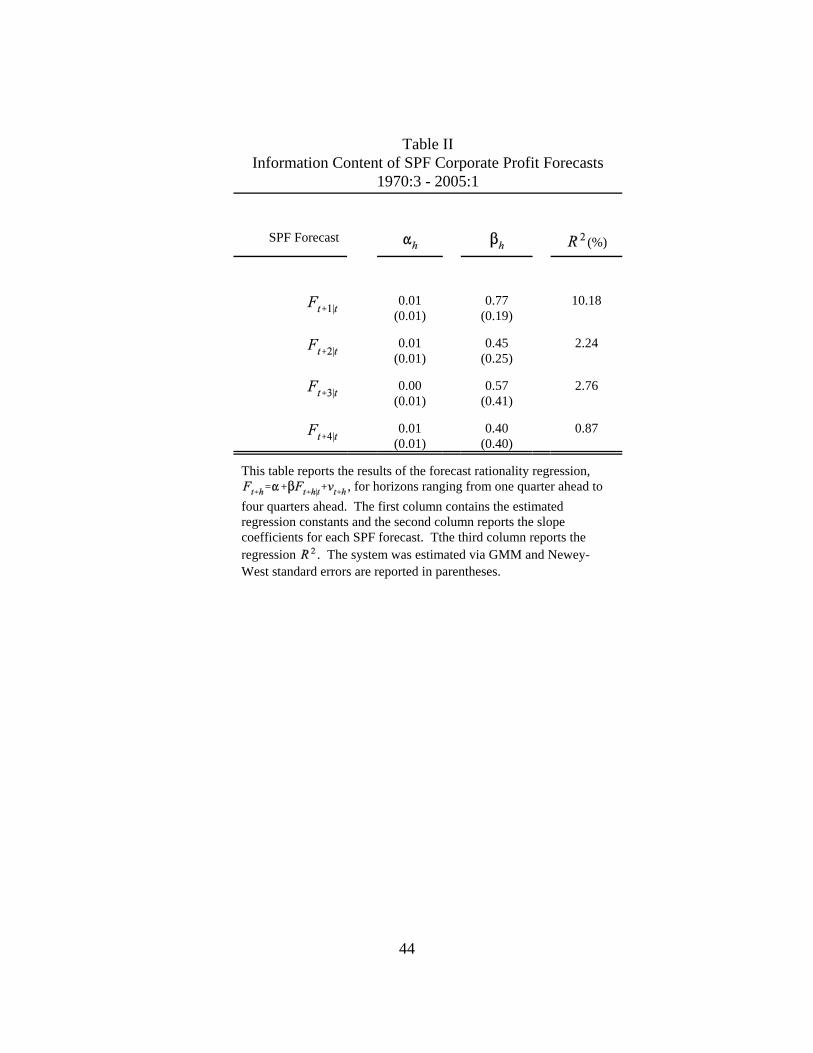
Turning to the results contained in Table II indicates that the SPF forecasts represent a

considerable improvement over and above the time series model. Each row of Table II contains

the estimates of and along with their standard errors and the associated regression .

Looking at the top row of Table II, one quarter ahead SPF forecasts have significant information

content for future corporate profit growth. Specifically, the one quarter ahead SPF forecasts

explain roughly 10% of the variation in NIPA corporate profits and the associated estimate of

5One can argue that the from the time series model should only be compared with that computed fromthe forecast error, , and not the regression from Table II. Two points are worth noting. First,

doing so lowers the from 10.2% to 9.3% in the case of the one step ahead forecasts. Second, Elliott, Kommunjerand Timmerman (2004) point out that the elicited forecast only has the interpretation of a conditional mean underquadratic loss. In the case that professional forecasters’ loss functions are not quadratic, interpreting as a

conditional mean is problematic and the from Table II may be a better measure of the forecast’s informationcontent than is the computed from . Moreover, in the case that the elicited forecast, , is a scaled version ofthe conditional mean, , it can still be informative about the revision process, .

10

is large and significant (0.77).5 As the forecast horizon lengthens, the information content of

the SPF forecasts naturally decline. At the two and three quarter ahead horizons, SPF forecasts

explain a little more than 2% of the variation in corporate earnings and the associated estimates

of and are smaller (0.45 and 0.57) and less significant. The forecasts, however, especially

in the case of two quarter ahead forecasts are informative about future profits when compared to

the benchmark AR(1) model. SPF forecasts of corporate earnings four quarters ahead have little

ability to account for future earnings growth since they explain less than 1% of the variation in

corporate profitability. Taken together, these results indicate that SPF forecasts are a useful

source of information about future movements in corporate profits. The forecasts are more

informative at shorter forecast horizons but are significantly more informative than forecasts

from a benchmark AR(1) model.

Aside from the question of how informative or accurate SPF forecasts are for future

corporate profits, it is also important to examine the extent to which the stock market reacts to

the news contained in these forecasts. This provides a market test of the SPF forecasts’

applicability as a measure of fundamental news. In particular, even if SPF forecasts were

excellent predictors of future earnings growth, if the stock market did not react to innovations in

the forecasts it would be difficult to interpret the forecasts as a source of fundamental news.

6 Returns are deflated using the CPI-U as a deflator.

11

Recall from the Campbell-Shiller decomposition of unexpected stock returns that,

,

so that in the event that return news is uncorrelated with fundamental news, the population

regression coefficient from regressing onto is unity. In order to assess the degree to

which the SPF expectation revisions are linked to real returns, I regress quarterly, real stock

returns on the CRSP value-weighted portfolio, , onto as well as each of its constituent

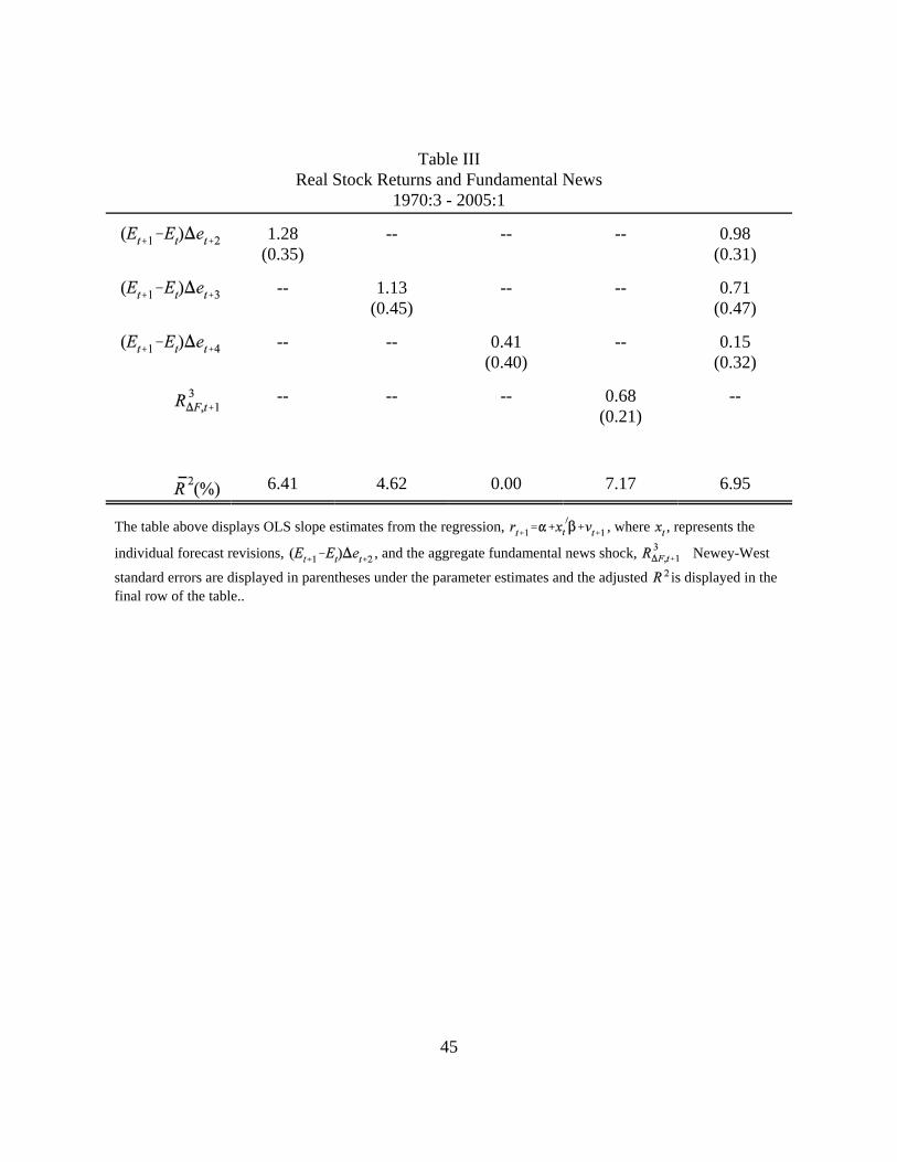
components, .6 The regression slope coefficients,

standard errors and adjusted are contained in Table III. Table III contains the results from

regressing each fundamental news measure onto real returns separately as well as the results

from regressing all three measures onto the real return series.

First, consider the reaction of the stock market to the individual SPF forecast revisions.

In the case of the first two revisions, , real stock returns react

strongly and significantly to changes in these profit forecasts. In both cases the point estimate of

the slope coefficient is slightly larger than one (1.28 ans 1.13) and highly significant. As the

length of the forecasting horizon increases the reaction of the stock market to forecast revisions

decreases. The reaction of real stock returns to the most distant SPF forecast

revisions, , is the smallest (0.40) and insignificant. Overall, however, real stock

returns do react significantly to SPF forecast innovations as expected. This is best seen by

12

examining the relationship between real returns and the measure of fundamental news, .

Positive fundamental news significantly increases real stock returns as evidenced by the large,

positive and significant slope estimate (0.68). It is also interesting to note that the fundamental

news measure summarizes well the information contained in all three revision series. The

adjusted in the regression of real returns on is larger than in any of the univariate

regressions or the multiple regression that uses each revision separately to explain real stock

returns.

The regression indicates that fundamental news accounts for a little more than 7% of

the variance in real stock returns over the sample period. This finding suggests that variation in

expected returns and return news dominates the effect of fundamental news in determining real

returns. While the amount of real return variation explained by fundamental news is small, this

finding is not unexpected. Previous studies linking movements in the stock market to

movements in fundamentals and movements in rates of return also find that movements in

fundamentals only explain a modest portion of stock return variability. Campbell (1991), for

example, finds that between 1952 and 1998, fundamental news explains between 8.5% to 10.0%

of the variance in stock returns. Recent studies by Bernanke and Kuttner (2004) as well as

Campbell and Vuolteenaho (2004), find similar results. Accordingly, the fact that the

constructed fundamental news series only explains around 7% of the variation in real stock

returns is consistent with the literature on the relation between fundamentals and stock returns.

In what follows, the revisions to SPF forecasts are used in conjunction with real stock

returns to construct an estimate of the two components of real stock returns that are related to

7Note that in defining , I subtract from rather than where is the OLS

slope estimate from Table III. One might reasonably prefer the latter. Since, however, the variance of is dominated by the variance of real returns, it makes little difference in the empirical analysis which way

is constructed.

13

expected returns and fundamentals. Namely, I construct the variables,

(II.7)

.7 (II.8)

Note that I do not take a stand on a model of expected returns to identify separately from

. This modeling choice is motivated by two considerations. First, there is much debate

and little agreement over what set of variables reliably predict stock returns. Second, much

empirical evidence indicates that the volatility of news to future returns dominates the volatility

of expected returns. As a result, the gain from directly modeling expected returns is likely to be

small. In what follows, I will use the term “return news” to refer to the term or its

estimate, . Similarly the term “fundamental news ” will refer to or its

estimate .

III. The Great Moderation and Stock Return Volatility: Fundamental and Return News

Structural Break Analysis

In order to assess the degree to which the three components of stock market volatility

14

were affected by the Great Moderation, I examine the evidence in favor of a structural break in

, and . Much of the literature on the Great Moderation has

interpreted the broad decline in the volatility of aggregate output, consumption, investment and

other macroeconomic aggregates as a permanent phenomenon. This has led previous researchers

to employ econometric tests of a single structural break as a means of testing for and

characterizing the size of the Great Moderation. Stock and Watson (2002) and McConnell and

Perez-Quiros (2000), for example, both employ single structural break tests in measuring the size

and significance of the Great Moderation. I employ a similar structural break test to remain

consistent with the permanent interpretation of the Great Moderation.

The structural break volatility model is specified is as follows,

, (III.1a)

, (III.1b)

where represents either or and the exponential model is employed to

account for the positivity of the absolute value. In order to assess the evidence in favor of a

structural break in the covariance between return news and fundamental news, I estimate the

structural break model,

, (III.1c)

. (III.1d)

In each case the break date, , must be constrained to lie away from the sample’s endpoints in

order to appeal to the asymptotic theory underlying the test. I selected the boundary points for

15

the break date following Andrews’ (1993) suggestion of using the middle 70% of the sample

period. The model is estimated for each possible break date within the boundary points by

GMM and the test statistic is defined to be the maximum Wald statistic over all possible break

dates of the null hypothesis that . Andrews (1993) provides the asymptotic distribution of

this test statistic, , under the null of no structural break. Using the boundary points referred

to above, the critical values of the test at the 10%, 5% and 1% level are 7.17, 8.85 and 12.35,

respectively.

I present the estimated break date, break size and its statistical significance in Table IV.

In Figure II, I display the value of the Wald statistic for each possible break date along with the

cutoff value for significance at the 10%, 5% and 1% level for each of the three tests. These plots

can be used to construct a confidence interval for the break date.

Looking at Figure II and Table IV the case for a permanent change in the volatility of

fundamental news, return news or the covariance between the two is strongest in the case of

fundamental news. In the case of fundamental news the structural break test is significant at a

level in between 1% and 5%. The estimated structural break parameter implies that the volatility

of fundamental news abated by roughly 50%. This is a large decline in volatility but generally in

line with the kind of volatility reduction that was experienced by other macroeconomic

aggregates over this period. As an example, Stock and Watson (2003) find that the volatility of

consumption and GDP growth declined by 40% after the onset of the Great Moderation. The

estimated break date of 1981:4 is also largely consistent with the timing of the Great Moderation.

While different authors use different dates for the Great Moderation all agree that the large

volatility decline occurred sometime in the early to mid-1980's. The case for a structural break

16

in the volatility of return news or the covariance between return news and fundamental news is

much weaker. While the estimated break date is within reason in both cases the test statistic is

well below the 10% critical value.

The results of the structural break tests indicate that the Great Moderation has affected

the volatility of fundamental news shocks. The structural break analysis suggests that the

volatility of fundamental news declined by roughly 50% since the onset of the Great Moderation.

In this sense, stock market volatility is related to macroeconomic volatility. Both

macroeconomic volatility and the volatility of fundamental news have declined in concert. The

strong link between macroeconomic volatility and fundamental news volatility, however, does

not carry over to return news. Since the volatility of fundamental news is small relative to the

volatility of return news, the Great Moderation did not exhibit a large influence on overall stock

return volatility.

These findings raise questions about how the fundamental news and return news

components of stock returns could react so differently to the same underlying structural change

in the macroeconomy. In what follows, I examine the effect the Great Moderation would have

from the perspective of Campbell and Cochrane’s (1999) habit formation asset pricing model.

Using this model, I show that the apparent disconnect between fundamental news volatility and

future return news volatility is entirely consistent with Campbell and Cochrane’s (1999) habit

formation model. This finding is further contrasted with the prediction of the traditional

CCAPM which predicts that a permanent decline in fundamental volatility would ultimately

result in a decline in stock return volatility.

17

IV. The Implications of the Great Moderation for Stock Market Volatility: An Asset

Pricing Model With Habit Formation

Motivation for the Modeling Framework

The main empirical finding of this paper is that while the volatility of fundamental news

has declined in response to the Great Moderation, the volatility of return news has not. From the

perspective of the Campbell-Shiller decomposition,

,

the volatility of return news, , has not been materially influenced by the large, abrupt and

arguably permanent drop in macroeconomic volatility since the middle of the 1980's. In this

section, I examine the influence of the Great Moderation on the different components of stock

return volatility through the lens of Campbell and Cochrane’s (1999) habit formation asset

pricing model (CCH). Specifically, I employ the CCH model and examine the effect of a one

time structural break in the volatility of consumption growth on the volatility of the different

components of real stock returns.

I choose to investigate the theoretical link between the volatility of fundamentals and

return news with the CCH model for two reasons. First, as an asset pricing model, CCH is

explicitly dynamic allowing for rich time variation in expected rates of return and hence provides

a substantive role for . In particular, even in an economy in which the distribution of

fundamentals, i.e. consumption or dividend growth, is fixed CCH delivers time variation in

expected rates of return. More traditional asset pricing models, such as the CCAPM, imply a

fixed rate of return when the distribution of fundamentals is fixed. As a result, absent any time

8There are variants of the CCAPM that do allow for time variation in expected rates of return through timevariation in the market risk premium. Lettau and Ludvigson (2001), for example, introduce time varying risk premiato the CCAPM. These models, however, are empirical and do not provide an equilibrium mapping between thedistribution of fundamentals and risk premia. As a result, it is not possible to examine the implications of the GreatModeration within the context of these models.

18

variation in the distribution of fundamentals, these models imply that return news, , is

identically zero. Time variation in expected rates of return can be added to these models by

introducing time variation in the distribution of fundamentals but these models then imply that

this is the only source of variation in expected rates of return. Since empirical evidence suggests

that time variation in expected rates of return, i.e. , is the main driver of stock return

volatility both before and after the onset of the Great Moderation, assuming that the Great

Moderation is the sole source of variation in expected rates of return is somewhat problematic.8

Alternatively, the richness of CCH implies that a variety of factors influence expected returns

and hence . As a result the CCH model provides a framework for disentangling the

importance of fundamental volatility relative to all other factors that drive expected returns.

Second, the CCH model is one of the few consumption based, rational asset pricing

models that captures a variety of stylized features of the U.S. stock market that have bedeviled

more traditional consumption based models for more than thirty years. In particular, CCH

delivers expected rates of return, risk free rates and Sharpe ratios that are consistent with

observed data. The large literature on the failure of the prototypical consumption based model,

i.e. the CCAPM, has shown that this model is largely unable to account for even the most

fundamental features of U.S. stock returns. Before conducting an analysis of the link between the

volatility of macroeconomic fundamentals and the volatility of stock returns it is desirable to

19

work with a model that can successfully account for the more basic features of U.S. stock

returns.

Before describing the model and how it behaves in the event of a Great Moderation in

consumption volatility, it is useful to point out the related work of Lettau, Ludvigson and

Wachter (2004) on the links between the stock market and the Great Moderation, as it is one of

the only other papers that assesses the effects of the Great Moderation on the stock market.

Their work differs from mine in several respects. First and foremost, Lettau, Ludvigson and

Wachter (2004) focus on the level of asset prices and not their volatility. Specifically, they focus

on whether or not the Great Moderation could account for the large run up in the level of stock

prices observed over the 1990's.

Also, their modeling strategy is considerably different from mine. There are three key

differences between our modeling strategies. First, they employ the CCAPM as their structural

model and I employ Campbell and Cochrane’s (1999) habit formation model. Second, they

model the Great Moderation as a transitory event in the sense that there is always a positive

probability of returning to a lower volatility regime. I follow the bulk of the Great Moderation

literature in interpreting the Great Moderation as a one time permanent decline in the volatility

of consumption growth. Lettau, Ludvigson and Wachter (2004) also model the volatility regime

as a hidden state that must be inferred from the observed history of consumption growth. In this

sense, learning plays a crucial role in their framework. I abstract from the effects of learning by

assuming that the structural break in fundamental volatility is observed immediately once it

occurs. Ultimately, the results of the analysis will suggest that including a learning process

would not materially change the predictions of the CCH model.

20

In what follows, I provide a brief description of the CCH model, how asset returns are

determined within the model and then I discuss how a one time break in the volatility of

consumption growth would affect the volatility of stock returns and its constituent components,

and .

The Campbell & Cochrane (1999) Habit Formation Model

The CCH model is a representative agent, complete markets endowment economy.

Below, I briefly describe the technology and preferences of the economy. The description

presented here is brief. Readers are referred to Campbell and Cochrane (1999) for a more

detailed description of the model.

Consumption growth is modeled as an exogenous process. The statistical model assumes

that log consumption follows a random walk with i.i.d. normally distributed shocks,

, (IV.1a)

, (IV.1b)

where represents the economy’s long-run growth rate and represents the level of uncertainty

surrounding future consumption. Since consumption is the only observable economic quantity

that relates to the broader macroeconomy, I consider the Great Moderation to be reflected in a

one time change in .

At this point it might be argued that the assumption on the consumption growth process

is inconsistent with the observed data from the SPF. In particular, if consumption, and

21

ultimately earnings and dividend, growth were i.i.d. then expectational terms of the form,

,

would be identically zero whereas the SPF clearly shows that these revisions to expectations are

non-zero. Importantly, however, CCH still provides a channel for fundamental news. In

particular, fundamental news is operative through the term which is non-zero in

the CCH model. A richer structure for revisions to expected future fundamentals could be

obtained within the CCH model by assuming an autoregressive structure for consumption

growth. While a variant of the CCH model in which consumption growth is autocorrelated

would be of interest, the substance of the analysis presented here would not be materially

affected by this change in the model’s structure.

Preferences in the CCH model are additively separable across time with discount factor,

. The model’s main departure from the standard consumption based model is in the

specification of per-period preferences, . In particular, each period, the investor’s utility is

defined with respect to a reference level of consumption, . Preferences take the form,

, (IV.2)

so that risk aversion is time varying. The coefficient of relative risk aversion, , takes the form,

,

22

where is defined to be the “surplus consumption ratio”. The reference level of

consumption, , is modeled as an external habit in the sense that the agent takes the reference

level as given and does not impute the effect of current choices on the future reference level.

Rather than model the evolution of the reference level directly, as in Constandinides (1990) for

example, a transformation of external habit, the log surplus consumption ratio is modeled as a

heteroskedastic, autoregressive process that reacts to shocks to consumption growth as follows,

, (IV.3)

where lowercase letters refer to logarithms of their uppercase counterparts. How the log surplus

consumption ratio, , responds to consumption shocks is governed by the sensitivity function,

. Importantly, note that the sensitivity of the future level of the log surplus consumption

ratio depends on its current level. The model for preferences is completed by specifying a

functional form for the sensitivity function.

Campbell and Cochrane (1999) require that the sensitivity function meet three separate

criteria: (1) real interest rates are a linear function of the log surplus consumption ratio; (2) the

reference level of consumption, , is pre-determined in the steady state so that, , when

; and (3) the reference level of consumption always moves non-negatively with

23

consumption. These three considerations yield the following specification of the sensitivity

function,

, (IV.4a)

, (IV.4b)

, (IV.4c)

where is a bound on the log surplus consumption ratio that ensures the sensitivity function

always remains positive and is the steady state value of the log surplus consumption ratio.

The Investment Opportunity Set in the Campbell-Cochrane Habit Formation Model

Before turning to an analysis of how changes in consumption volatility will affect stock

market volatility, it is useful to characterize the investment opportunity set in the CCH model.

An understanding of how macroeconomic risk affects the investment opportunity set will

provide some insight into how changing macroeconomic risk will affect the volatility of stock

returns. In order to have intuition for how macroeconomic risk affects the investment

opportunity set it is useful to consider how macroeconomic risk affects the model’s stochastic

discount factor (SDF).

The stochastic discount factor in the CCH model takes the particularly simple form,

9In what follows, I will interchangeably refer to and as the stochastic discount factor.

24

, (IV.5)

or in its log form,

, (IV.6)

and this representation of the model’s SDF makes clear how CCH differs from more traditional

asset pricing models such as the CCAPM.9 In the CCAPM the stochastic discount factor is

solely identified with consumption growth, . CCH augments the SDF with the change

in the log-surplus consumption ratio. Also, note that this additional factor, , is directly linked

to the underlying macroeconomy in the sense that movements in and are perfectly

conditionally correlated given the law of motion for . The conditional mean and variance of

the log SDF, determine both risk free rates and Sharpe ratios in the economy. They are given by,

, (IV.7)

, (IV.8)

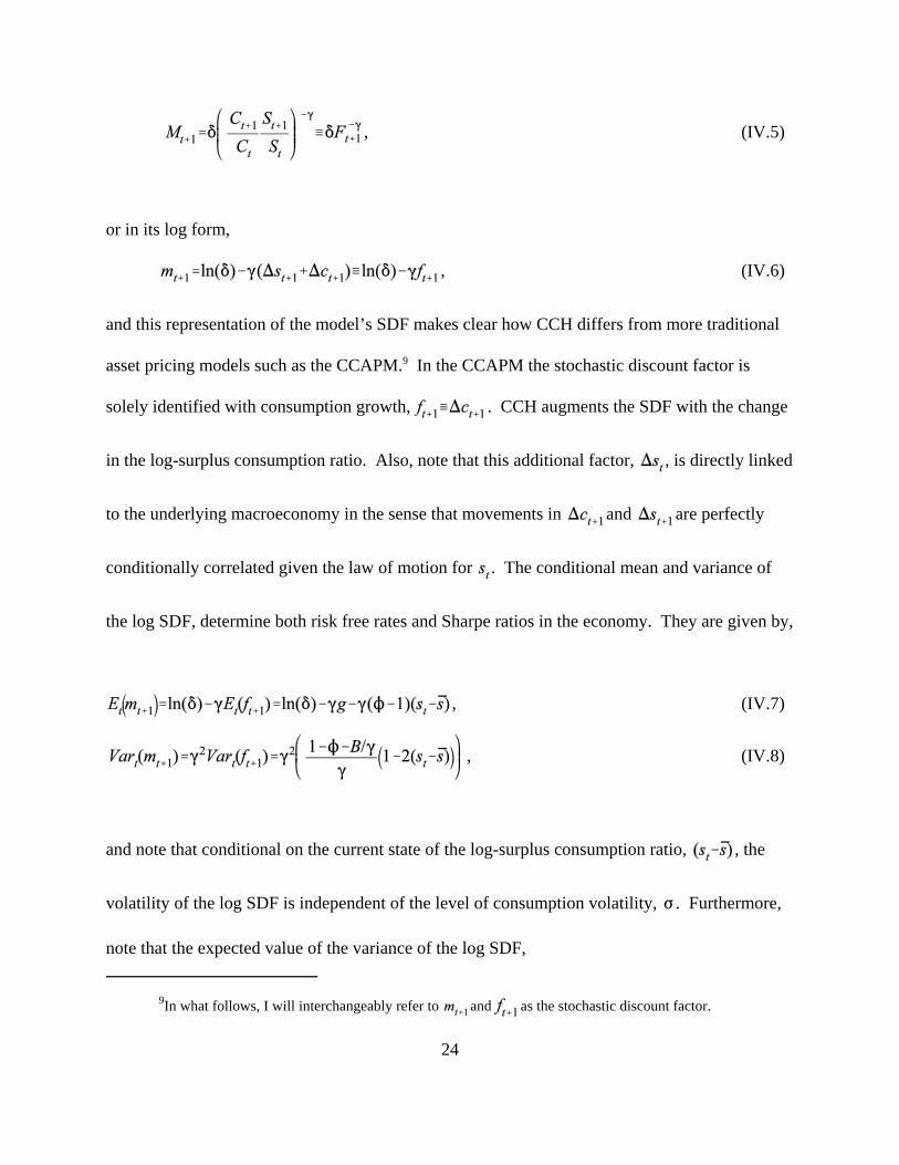
and note that conditional on the current state of the log-surplus consumption ratio, , the

volatility of the log SDF is independent of the level of consumption volatility, . Furthermore,

note that the expected value of the variance of the log SDF,

25

,

is itself independent of the level of consumption volatility. This feature of the CCH model’s

stochastic discount factor stands in stark contrast to other, more traditional, asset pricing models.

More traditional asset pricing models, such as the CCAPM, directly link the SDF with

consumption growth, , so that there is a direct relationship between the

volatility of consumption and the volatility of the SDF.

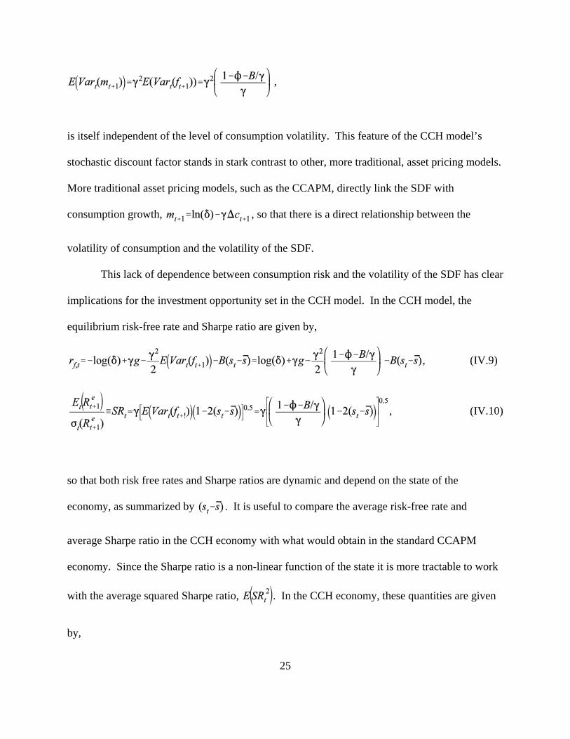
This lack of dependence between consumption risk and the volatility of the SDF has clear

implications for the investment opportunity set in the CCH model. In the CCH model, the

equilibrium risk-free rate and Sharpe ratio are given by,

, (IV.9)

, (IV.10)

so that both risk free rates and Sharpe ratios are dynamic and depend on the state of the

economy, as summarized by . It is useful to compare the average risk-free rate and

average Sharpe ratio in the CCH economy with what would obtain in the standard CCAPM

economy. Since the Sharpe ratio is a non-linear function of the state it is more tractable to work

with the average squared Sharpe ratio, . In the CCH economy, these quantities are given

by,

26

, (IV.11)

, (IV.12)

which contrasts sharply with the corresponding expressions in the standard CCAPM economy,

, (IV.13)

, (IV.14)

since consumption risk plays no role in determining average risk free rates and Sharpe ratios in

the CCH economy but plays a direct role in the CCAPM economy.

The average risk free rate and Sharpe ratio in the CCH model can be thought of as the

risk-free rate and Sharpe ratio that would obtain under the traditional CCAPM if consumption

growth were distributed according to,

,

rather than,

.

In this way, CCH replaces consumption risk with something that might be termed “habit risk” in

the sense that the fundamental volatility that drives Sharpe ratios and risk-free rates only

depends on preference parameters.

The replacement of consumption risk with habit risk in the CCH model is central to its

27

success as an asset pricing model. This is precisely the sense in which Campbell and Cochrane

(1999) claim that their model “posits a fundamentally novel description of risk premia”. As the

authors put it, “[i]nvestors fear stocks primarily because they do poorly in recessions unrelated to

the risks of long-run average consumption growth”. The defining characteristic of the equity

premium puzzle is that consumption growth is not volatile enough to explain either the relatively

high Sharpe ratios of U.S. stock returns or the low real risk-free rates of interest observed in

post-WWII data. Essentially, this fundamental source of risk is simply not risky enough to

account for the high equity premia observed in the data. By introducing the notion of surplus

consumption, , CCH introduces a new source of risk in the economy that is able to account for

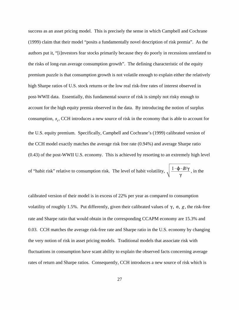
the U.S. equity premium. Specifically, Campbell and Cochrane’s (1999) calibrated version of

the CCH model exactly matches the average risk free rate (0.94%) and average Sharpe ratio

(0.43) of the post-WWII U.S. economy. This is achieved by resorting to an extremely high level

of “habit risk” relative to consumption risk. The level of habit volatility, , in the

calibrated version of their model is in excess of 22% per year as compared to consumption

volatility of roughly 1.5%. Put differently, given their calibrated values of , the risk-free

rate and Sharpe ratio that would obtain in the corresponding CCAPM economy are 15.3% and

0.03. CCH matches the average risk-free rate and Sharpe ratio in the U.S. economy by changing

the very notion of risk in asset pricing models. Traditional models that associate risk with

fluctuations in consumption have scant ability to explain the observed facts concerning average

rates of return and Sharpe ratios. Consequently, CCH introduces a new source of risk which is

28

both quite large relative to consumption risk, and more importantly from the perspective of this

paper, unrelated to the riskiness of observable macroeconomic quantities such as consumption or

output. Ultimately, the lack of a direct link between the riskiness of the stock market and the

riskiness of macroeconomic fundamentals, i.e. consumption, in the CCH model has direct

consequences for the relation between macroeconomic and stock market volatility.

Stock Return Volatility and the Great Moderation in the CCH Model

In this section I examine how a one-time permanent decline in the volatility of

consumption growth affects the volatility of the stock market in the CCH model. I consider the

variant of CCH in which a share of stock is a claim to consumption. Specifically, I assume that

dividends coincide with consumption in the model so that, . Alternatively, one could

model stocks as a claim on dividends that are imperfectly correlated with consumption growth so

that, . In this case, modeling the Great Moderation would amount to a significant

decline in both consumption volatility, , as well as a proportional decline in the volatility of the

idiosyncratic component of dividend growth, . Also, I assume that the change in consumption

volatility is not anticipated before it occurs and is fully realized once it occurs. In this sense, I

abstract from the effects of any learning or transitional dynamics. As a result, I employ a

comparative static analysis across a high and low consumption volatility economy to summarize

the likely effects of a structural break in consumption volatility within a single economy. I

analyze the effect of a Great Moderation in consumption volatility on stock return volatility by

analyzing the effect of a decline in consumption volatility on the volatility of stock dividends

29

and the volatility of the price dividend ratio. I then solve and simulate the CCH model for two

different levels of consumption volatility and compare the characteristics of the resulting

equilibria.

Consider the following decomposition of single period real stock returns,

,

or in logs,

,

so that the stock return may be thought of in terms of the dividend flow and the change in the

stock’s price-dividend ratio. Within the context of Campbell and Shiller’s (1988a,b)

decomposition the unexpected return can be written as,

.

Since consumption and dividend growth is i.i.d. in this model, stock prices contain no

information about future dividend growth. As a result, the component of unexpected returns due

to changes in the price-dividend ratio can be solely identified with . This implies that the

shock to dividends and shock to future returns can be identified as,

, (IV.15)

. (IV.16)

Accordingly, analyzing the effect of a Great Moderation on stock return volatility within the

30

CCH model amounts to analyzing how a change in the volatility of consumption growth affects

the volatility of and .

In the case of news about fundamentals, , the effect is immediate. A

reduction in consumption growth volatility directly translates, one for one, into a reduction in the

volatility of . The effect of declining consumption growth volatility on the volatility

of the price-dividend ratio is less direct.

Campbell and Cochrane (1999) show that the equilibrium price-dividend ratio in the

CCH economy is only a function of the state, . Specifically, the price-dividend ratio

satisfies the following functional equation,

, (IV.17)

where the expectation is taken with respect to the future state. While an analytical expression for

does not exist, Campbell and Cochrane (1999) demonstrate that the function is nearly a

log-linear function of ,

, (IV.18)

so that the volatility of the (log) price-dividend ratio roughly corresponds to the product of the

10 Following Campbell and Cochrane (1999), I solve and simulate the model at the monthly frequency. Iuse the same parameter transformations between the annual and monthly frequency used by Campbell and Cochrane(1999). The model was solved and simulated using GAUSS computer code provided by the authors. The GAUSScode may be downloaded from,http://gsbwww.uchicago.edu/fac/john.cochrane/research/Data_and_Programs/habit%20programs.

31

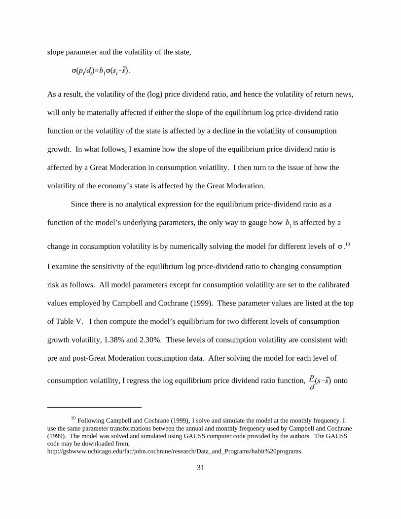
slope parameter and the volatility of the state,

.

As a result, the volatility of the (log) price dividend ratio, and hence the volatility of return news,

will only be materially affected if either the slope of the equilibrium log price-dividend ratio

function or the volatility of the state is affected by a decline in the volatility of consumption

growth. In what follows, I examine how the slope of the equilibrium price dividend ratio is

affected by a Great Moderation in consumption volatility. I then turn to the issue of how the

volatility of the economy’s state is affected by the Great Moderation.

Since there is no analytical expression for the equilibrium price-dividend ratio as a

function of the model’s underlying parameters, the only way to gauge how is affected by a

change in consumption volatility is by numerically solving the model for different levels of .10

I examine the sensitivity of the equilibrium log price-dividend ratio to changing consumption

risk as follows. All model parameters except for consumption volatility are set to the calibrated

values employed by Campbell and Cochrane (1999). These parameter values are listed at the top

of Table V. I then compute the model’s equilibrium for two different levels of consumption

growth volatility, 1.38% and 2.30%. These levels of consumption volatility are consistent with

pre and post-Great Moderation consumption data. After solving the model for each level of

consumption volatility, I regress the log equilibrium price dividend ratio function, onto

32

the log state, using 18 discrete points, . In Table V, I present the underlying

model parameters used in solving the CCH model as well as the parameters from the OLS

regression,

,

along with the regression .

Looking at the listed in Table 5 for both the low and high volatility model

specification shows that the linear approximation is not overly restrictive. In each case the is

in excess of 99% indicating that the log linear approximation is appropriate. Looking at the

constant and slope terms, both of the estimated equilibrium price-dividend ratio functions are

nearly identical. This result is driven by the fact that the stochastic discount factor, , the

fundamental driver of stock returns in the model is not affected by the change in consumption

volatility. In this sense, stock returns are as risky in a low consumption volatility as in a high

consumption volatility environment. Since the risk inherent in owning stocks does not change as

consumption risk changes, the level and slope of the equilibrium price-dividend ratio is

unaffected by a Great Moderation in consumption volatility.

Turning to the volatility of the state of the economy, , it is useful to recall how the

state of the economy is related to the SDF. Namely,

,

so that,

33

.

The effect of a change in macroeconomic volatility, , on the state of the economy can be

analyzed by appealing to the above equation. Recall that the conditional variance of the

stochastic discount factor, , is independent of the level of macroeconomic volatility. As a

result, changing macroeconomic risk only affects the volatility of the state of the economy

through the term . Formally we have that,

, (IV.19)

where the above expression uses the fact that the stochastic discount factor and consumption

growth are perfectly conditionally correlated. Finally, taking the derivative of this expression

with respect to yields,

, (IV.20)

so that reducing macroeconomic volatility will actually increase the volatility of the state

whenever exceeds .

Finally, recall that the average volatility of in Campbell and Cochrane’s (1999)

calibrated version of the model is in excess of 20%. Accordingly, reducing macroeconomic

volatility actually increases the volatility of the state. Moreover, as discussed previously, the

high level of volatility in is required to match the stylized facts of the US stock market.

Accordingly, versions of the CCH model in which the volatility of is less than would be

34

unable to account for the observed high average Sharpe ratios and low risk free rates observed in

the US economy. Consequently, parameterizations of the CCH model that are consistent with

the basic stylized facts of the U.S. stock market predict that the volatility of the economy’s state

and hence the volatility of return news shocks will only increase in the face of a large decline in

macroeconomic volatility.

In order to provide a quantitative assessment of the effect of a large decline in

consumption volatility consistent with the Great Moderation, I solve and then simulate the CCH

model for 100,000 months. The model is solved and simulated for both high and low

consumption growth volatility. I employ the same sets of parameter values that were used to

analyze the behavior of the equilibrium price-dividend ratio. In Table 6, I report the mean,

standard deviation and first order autocorrelation of different model variables across the two

economies. All numbers are reported in annualized terms.

I display the model’s fundamental, exogenous, driving variables in the top panel of Table

6. Consumption growth, , has a constant mean of 1.9% per annum and its standard deviation

changes from 2.30% to 1.38% resulting in a 40% decline. Looking at the change in the state

variable, , indicates that across the two economies there is little difference in the volatility of

the state variable even though there is a large difference in the volatility of consumption growth.

Consistent with the previous analysis, the standard deviation of the state variable increases

slightly from 0.225 to 0.233. Looking at the model’s SDF, , it is apparent that its riskiness is

unaffected by the Great Moderation. The volatility of the model’s stochastic discount factor and

hence the riskiness of the stock market is not materially affected by a significant decline in

35

fundamental macroeconomic volatility.

In the middle panel of Table 6, I compare the financial market equilibria of the high and

low consumption growth volatility economies. In both economies the average Sharpe ratio is

both high and highly variable. Across the two economies, however, there is only a minor

difference in both the average level of the Sharpe ratio and its volatility. The lack of any

difference in the behavior of the Sharpe ratio across the two economies is consistent with the

earlier theoretical analysis. The level of the Sharpe ratio is determined by the amount of

variability in which is shown to be nearly identical across the two economies. The time-

variation in the Sharpe ratio is driven by time-variation in the state, . Since the distribution of

the underlying state variable does not differ appreciably across the two economies neither do the

stochastic properties of the Sharpe ratio.

The average volatility of stock returns across both economies is also very similar. The

average conditional standard deviation of returns, is 13.7% per year in the low volatility

economy and 14.2% per year in the high volatility economy. Also, the temporal dependence in

volatility is largely unaffected by the large change in consumption volatility. In both cases the

first order autocorrelation in volatility is roughly 99%. Looking at the different components of

stock return volatility, the majority of stock volatility is accounted for by variation in return

news across both economies. Across both economies, return news explains over 90% of the

volatility of stock returns. As a result, the fact that fundamental news volatility declines by 40%

between the high and low volatility economies has essentially no effect on stock market

volatility.

36

The simulation results of the CCH model indicate that changing consumption risk only

has minor consequences for stock market volatility. In particular, though the volatility of

fundamental news is affected by the Great Moderation, the volatility of return news is essentially

unaffected by a large decline in consumption volatility. Consistent with the previous analysis,

the volatility of return news actually increases slightly following the Great Moderation. Since

the bulk of stock market volatility is attributable to return news variation, the Great Moderation

does not exhibit an appreciable influence on total stock market volatility.

These features of the CCH model are remarkably consistent with the pattern in stock

market volatility that has been observed over the period of the Great Moderation. The

previously reported empirical results indicate that fundamental news has declined substantially

since the onset of the Great Moderation. Specifically, the volatility of the SPF fundamental

news series has declined by 50% since the third quarter of 1981. Over the same period, the

volatility of measured return news has not abated. Empirically, the large reduction in

fundamental news volatility has not spilled over into the volatility of return news. The CCH

model provides a framework for interpreting these findings. In the CCH model, the risk inherent

in the stock market is unrelated to long term economic risk. Accordingly, changes to the

volatility of macroeconomic fundamentals such as consumption have no discernible effect on the

riskiness, and hence volatility, of the stock market.

V. Conclusion

The large and persistent decline in macroeconomic volatility that has occurred since the

middle of the 1980's represents one of the single largest changes to the macroeconomic

37

landscape in the past twenty years. In this paper, I document how this Great Moderation in

macroeconomic volatility has affected stock market volatility. Furthermore, I show that the

experience thus far is consistent with a rational, consumption based asset pricing model.

The empirical results show that the Great Moderation has had very different influences

on the two fundamental components of stock returns. The volatility of news about stock

fundamentals, such as dividends, earnings or cash flow, have abated since the onset of the Great

Moderation. In particular, the volatility of fundamental news shocks has declined by roughly

50% since the fourth quarter of 1981. The size of this reduction in volatility is consistent with

the reduction in the volatility of a broad range of macroeconomic aggregates including real

output and consumption growth over the same period. These findings indicate that the volatility

of macroeconomic fundamentals share important links with the volatility of the component of

stock returns that is directly related to news about fundamentals.

In contrast to the empirical findings on the links between fundamental news and

macroeconomic volatility I find no significant link between macroeconomic volatility and the

volatility of return news. The divergence in behavior between fundamental and return news is

reconciled with Campbell and Cochrane’s (1999) habit formation asset pricing model. The CCH

model predicts that even very large changes in consumption and dividend volatility will only

have negligible effects on return news volatility and ultimately overall stock return volatility. In

this way, the CHH model provides a framework for reconciling the disparate trends in the

volatility of real activity and the stock market.

The divergence between the behavior of fundamental news and return news shocks

within the context of the CCH model derives from the model’s stance on the underlying nature

38

of stock market risk. Unlike the CCAPM, the risk of declining consumption is not the most

important source of risk in the CCH economy. Declining surplus consumption, rather than

declining consumption is the dominant source of stock market risk in the CCH economy. More

importantly, the risk associated with surplus consumption is largely unaffected by changes in

consumption risk. As a result, reductions in consumption volatility do not make stocks less risky

and stock market volatility does not decline in response to a Great Moderation in consumption

volatility.

39

References

Bernanke B., and Kuttner K. (2004), “What Explains the Stock Market’s Reaction to Federal

Reserve Policy,” Finance and Economics Discussion Series Working Paper, 2004-16,

Board of Governors of the Federal Reserve.

Campbell J. (1991), “A Variance Decomposition for Stock Returns,” The Economic Journal,

101, 157-179.

Campbell J. and Cochrane (1999), “By Force of Habit: A Consumption-Based Explanation of

Aggregate Stock Market Behavior,” Journal of Political Economy, 107, 205-251.

Campbell J., and Shiller R. (1988a), “The Dividend Price Ratio and Expectations of Future

Dividends and Discount Factors,” Review of Financial Studies, 1, 195-227.

Campbell J., and Shiller R. (1988b), “Stock Prices, Earnings and Expected Dividends,” Journal

of Finance, 43, 661-676.

Campbell J., and Vuolteenaho T. (2004), “Bad Beta, Good Beta,” American Economic Review,

94(5), 1249-1275.

Constandinides G. (1990), “Habit Formation: A Resolution of the Equity Premium Puzzle,” The

Journal of Political Economy, 98, 3, 519-543.

Croushore D. (1993), “Introducing the Survey of Professional Forecasters,” Federal Reserve

Bank of Philadelphia Business Review, Nov/Dec.

Elliott G., Komumjer I., and Timmerman A. (2004),” Biases in Macroeconomic Forecasts:

Irrationality or Asymmetric Loss?,” working paper, UCSD.

Kim C., and Nelson C. (1999), “Has the U.S. Economy Become More Stable? A Bayesian

Approach Based ona Markov-Switching Model of the Business Cycle,” Review of

40

Economics and Statistics, 81,4,608-616.

Lettau M., and Ludvigson S. (2001), “Resurrecting the (C)CAPM: A Cross Sectional Test When

Risk Premia are time Varying,” Journal of Political Economy, 109, 6, 1238-1287.

Lettau M., Ludvigson S., and Wachter J. (2004), “The Declining Equity Premium: What Role

Does Macroeconomic Risk Play?,” working paper, New York University.

McConnell M., and Perez-Quiros G. (2000), “Output Fluctuations in the United States: What

Has Changed Since the Early 1980's?,” American Economic Review, 90, 5, 1464-1476.

Schwert W. (1989), “Why Does Stock Market Volatility Change Over Time?,” Journal of

Finance, 44, 1115-1153.

Schwert W. (1990), “Stock Market Volatility,” Financial Analysts Journal, May-June, 23-34.

Stock J., and Watson M. (2002) “Has the Business Cycle Changed and Why?,” NBER

Macroeconomics Annual, ed. M. Gertler and K. Rogoff, Cambridge: National Bureau of

Economic Research.

Stock J., and Watson M. (2003) “Has the Business Cycle Changed? Evidence and Explanations,”

FRB Kansas City Symposium 2003

41

The above figure displays, , constructed from the Survey of ProfessionalForecasters (SPF) between 1970:3 and 2004:4. Specifically, , is identified with the growth in real corporateprofits after taxes. The shaded regions depict the NBER recession dates.

-.15

-.10

-.05

.00

.05

.10

.15

1970 1975 1980 1985 1990 1995 2000 2005

Fundamental News

Qua

rterly

New

sFigure I

Fundamental News from the SPF1970:3 - 2004:4

42

The above figure displays the series of F-statistics that are used to determine for the Andrews’ (1993)structural break test. The horizontal lines represent the 1%, 5% and 10% critical values respectively. For eachseries, the F-statistic was computed for each break date between 1975:3 through 2000:1.

0

2

4

6

8

1 0

1 2

1 4

1 9 7 5 1 9 8 0 1 9 8 5 1 9 9 0 1 9 9 5 2 0 0 0 2 0 0 5

F u n d a m e n ta l N e w s V o la t i l i t y

F-S

tatis

tic

0

2

4

6

8

1 0

1 2

1 4

1 9 7 5 1 9 8 0 1 9 8 5 1 9 9 0 1 9 9 5 2 0 0 0 2 0 0 5

R e tu rn N e w s V o la t i l i t y

F-S

tatis

tic

0

2

4

6

8

1 0

1 2

1 4

1 9 7 5 1 9 8 0 1 9 8 5 1 9 9 0 1 9 9 5 2 0 0 0 2 0 0 5

F u n d a m e n ta l N e w s a n d R e tu rn N e w s C o va ria n c e

F-S

tatis

tic

Figure IIVolatility Structural Break Tests

Fundamental News and Return News

43

Table IEarnings Forecast Revisions and Fundamental News

Summary Statistics1970:3 - 2005:1

Mean -0.001 -0.004 0.003 -0.003

Median 0.000 -0.001 0.003 0.001

Std. Dev. 0.019 0.018 0.016 0.037

Skewness -0.500 -0.856 0.400 -0.795

Kurtosis 7.205 5.000 6.855 5.283

Jarque-Bera 108.180

(0.000)

40.169

(0.000)

89.706

(0.000)

44.841

(0.000)

The table above displays various summary statistics for each of the expectation revisions and for the fundamentalnews series. The Jarque-Bera statistic tests the null hypothesis that the data is distributed normally. Theasymptotic p-value of the test is displayed below the statistic in parentheses.

44

Table IIInformation Content of SPF Corporate Profit Forecasts

1970:3 - 2005:1

SPF Forecast (%)

0.01(0.01)

0.77(0.19)

10.18

0.01(0.01)

0.45(0.25)

2.24

0.00(0.01)

0.57(0.41)

2.76

0.01(0.01)

0.40(0.40)

0.87

This table reports the results of the forecast rationality regression,, for horizons ranging from one quarter ahead to

four quarters ahead. The first column contains the estimatedregression constants and the second column reports the slopecoefficients for each SPF forecast. Tthe third column reports theregression . The system was estimated via GMM and Newey-West standard errors are reported in parentheses.

45

Table IIIReal Stock Returns and Fundamental News

1970:3 - 2005:1

1.28(0.35)

-- -- -- 0.98(0.31)

-- 1.13(0.45)

-- -- 0.71(0.47)

-- -- 0.41(0.40)

-- 0.15(0.32)

-- -- -- 0.68(0.21)

--

6.41 4.62 0.00 7.17 6.95

The table above displays OLS slope estimates from the regression, , where , represents the

individual forecast revisions, , and the aggregate fundamental news shock, Newey-West

standard errors are displayed in parentheses under the parameter estimates and the adjusted is displayed in thefinal row of the table..

46

Table IVStructural Breaks in Fundamental News and Return News Volatility

1970:3 - 2005:1

Dependent Variable

1981:4 -3.76(0.16)

-0.70(0.20)

0.50 11.75**

1976:2 -2.92(0.14)

-0.31(0.20)

0.27 2.34

1983:3 0.003(0.001)

-0.002(0.001)

-- 2.98

The table above displays estimates from the structural break model, ,

. The model is estimate via GMM and Newey-West standard errors are reported in parenthesesunder the parameter estimates. The statistic, , is a formal test for a single structural break and it is asymptoticdistribution is given by Andrews (1993). *** signifies significance at the 1% level, ** signifies significance at the5% level and * signifies significance at the 10% level.

47

Table VCCH Equilibrium Log Price-Dividend Ratio Functions

Low vs. High Consumption Volatility

ModelParameters

1.89% 0.94% 0.87 2.00 0.00

ConsumptionVolatility

5.59 0.56 0.99

5.62 0.56 0.99

The top panel of this table displays the model parameters used in numerically solving for the equilibrium log price-dividend ratio as a function of the log state, . The bottom panel shows the result from fitting the equilibriumlog-price dividend ratio function to a linear function using OLS. The parameters represent the constant and

slope parameters, respectively. The summarizes the fit of the linear approximation.

48

Table VIThe Great Moderation and the CCH Model

Model Characteristics

Mean Standard Deviation Autocorrelation

Fundamental Variables

0.019 0.019 0.023 0.014 -0.001 -0.001

0.000 0.000 0.225 0.233 -0.007 -0.007

0.019 0.019 0.245 0.246 -0.007 -0.007

Financial Variables

0.067 0.066 0.151 0.146 -0.006 -0.006

0.071 0.070 0.014 0.014 0.991 0.991

0.000 0.000 0.023 0.014 -0.001 -0.001

0.000 0.000 0.128 0.133 -0.001 -0.001

0.142 0.137 0.049 0.051 0.988 0.988

0.376 0.374 0.182 0.190 0.990 0.990

Valuation Variables

3.066 3.094 0.272 0.282 0.991 0.991

22.181 22.853 5.129 5.435 0.977 0.976

The table above reports the mean, standard deviation and first order autocorellation in several model characteristicsfrom the CCH model using a high value, 2.3%, and a low value, 1.9%, of consumption volatility. In each case themodel was simulated for 100,000 periods. The other model parameters are fixed at the values reported in Table 5. All numbers are reported in annualized terms.