Student

Spring 2011

Master Thesis, 15 ECTS

Master’s Program in Economics, 120 ECTS

Stock Market Co-Movement and Volatility Spillover between USA and South Africa

Manex Yonis

ii

Acknowledgements

First and for most, I would like to forward my thanks to my supervisors Kurt Brännäs and

Yuna Liu for the encouragement and guidance that they provided during the writing of this

thesis. Through all this, however, it is beyond my expression to thank my family for their

patient and advice; thank you. Finally, I would like to express my deepest gratitude to Hasete

for reminding me to get it done.

iii

Abstract

The purpose of this study is twofold. First, I look at the co-movement of the US and South

African stock markets. Second, I examine the existence of volatility spillover between them. I

estimate unrestricted bivariate GARCH-BEKK representation proposed by Engle and Kroner

(1995) and VAR model by using daily total return series. I find evidence of return spillover

from NYSE to JSE by analyzing VAR based on two lags. While analyzing the MA-GARCH

model, empirical results exhibit that volatility spillover between US and SA is persistence.

Uni-directional link regarding transmission of shocks and volatility persistence between NYSE

and JSE is revealed, the direction is from NYSE to JSE, as off-diagonal parameters a12 and g12

are statistically significant. Finally, a strong influence of US market is observed in this paper

regarding stock movement in the SA market.

Key Words: Financial Globalization, Financial Crisis, Volatility Spillover, MA-GARCH,

Unrestricted Bivariate BEKK-GARCH Model.

iv

Table of Contents

Abstract iv

1. Introduction 1

1.1. Background 1

1.2. Objective 3

1.3. Scope and Limitations 3

1.4. Data and Methodology 3

1.5. Organization of The Paper 4

2. Literature Review 5

2.1. Theoretical Review 5

2.1.1. Financial Globalization 5

2.1.2. Financial Crisis 6

2.1.3. Volatility 8

2.2. Empirical Review 10

2.2.1. Stylized Facts of Financial Time Series Data 10

2.2.2. Empirical Literature 11

3. Econometric Method 13

3.1. Conditional Heteroskedasticity 13

3.2. BEKK-GARCH Representation 15

3.3. Vector Autoregression Model 17

3.4. Estimation 17

4. Data and Descriptive Statistic 18

5. Empirical results 21

5.1. VAR Estimation 21

5.2. MA-GARCH BEKK Estimation 23

6. Conclusion and Further Studies 26

References 27

v

Appendices

Tables

1. Estimated parameters for the mean return model 31

2. Estimated parameters for full BEKK MA-GARCH

presentation 32

3. Estimated Parameters for MA (1) 33

4. Correlations 33

Figures

1. Stock Indices 34

2. Frequency distribution of NYSE and JSE daily return series 35

3. Estimated conditional variance of NYSE and JSE

by unrestricted BEKK Model 36

Unrestricted Version of bi-variate MA-GARCH BEKK 37

1

1. Introduction

1.1. Background

The substantial increase in global financial flows along with the increasing globalized

economic activity has resulted in increased interdependence of major financial markets all

over the world (Balios and Xanthakis, 2003 pp 106). The interdependence of stock markets

has potential benefits that could boom investment and in turn economic growth (Mishkin,

2005 pp 14). Nevertheless, interdependence is accompanied with greater ease and speedy

transmission of volatility shocks in markets. The flow of, almost costless information,

reduced the isolation of domestic markets and increased their ability to react promptly to

news and shocks originating from the rest of the world (Singh & Kumar, 2008). This enables

volatility from global stock market to affect volatility in domestic capital market.

Accordingly, this interdependence between the global financial markets makes investors

and portfolio managers to have a close watch on the movement of not only the domestic

markets but also the international markets in order to carefully plan their global investment

strategy. Besides, policy makers are also interested whether a stock market show signs of co-

movement with other global market because the volatility spillover to that market has an

impact on the smooth functioning of the financial system and in turn the economic

performance (Mishkin 2005 pp 27).

Scholars in the field have been trying the corridor that can express the transmission

mechanism and degree of volatility spillover between financial markets. Accordingly, many

models and hypothesis has been studied extensively in recent years. Despite the level of

severity, many of them has been reached in common consensus that a result of intense

volatility somewhere in the global financial market, the dominant one, will spillover through

other financial markets (Kim and Rogers, 1995).

There are several studies focusing on the stock market linkage across countries. For instance,

Kim and Rogers (1995) found existence of volatility spillover from two well developed

financial centers, USA and Japan, to Korea after the announcement of liberalization. The

great influence of US market on UK and Japans market through return co-movement was

found by the work of Connolly and Wang (2000). Research by Surya (2009) found that there

2

is significant volatility spillover effect from USA and Japan markets to Indonesia. Sariannidis

et al (2010) found that there is positive co-movement between the financial markets of Hong

Kong, India and Singapore. They also found the integration of these markets derived from

common information which mostly stemmed from the US market. Moreover, the strong

impact of high degree shocks in NYSE and RTS on volatility and return of Baltic state stock

markets was shown in the thesis of Soultanaeva (2011).

However, considerably, little has been done in volatility spillover and return co-movement

between developed markets and emerging African markets. South Africa has the most

powerful economy in the continent of Africa and plays a leading role in industrial output,

mineral production and supplying a large proportion of Africa´s electricity. According to the

KOF index of globalization for 2011, South Africa has the second most economically

globalized economy in Africa and which is ranked 55 out of 186 nations around the world.

The size of the South African equity market is quite small as compared to that of the US.

However, since, a number of South African firms are also listed on the US stock exchanges

such as the NYSE; there is a chance of volatility and return spillover among these two

markets.

Volatility is a measure of uncertainty about future asset price or return change. Since it is a

major measure of risk for modern financial theories, it is a significant input for analyses in

risk management, strategic financial planning and policy driving. The motivation for my

paper is trying to answer a question of; are there significant volatility interactions in the

form of co-movement and spillover between USA and South Africa by focusing on

interaction of intraday returns and volatility.

The study considers volatility spillover modeling by using the bivariate BEKK-GARCH model

proposed by Engle and Kroner (1995). This BEKK formulation enables us to study the possible

transmission of volatility from one market to another, as well as any increased persistence in

market volatility (Engle, 1990). Besides, Vector Autoregression (VAR) lags method is applied

to capture return spillover and the interdependence of one market on the other.

3

1.2. Objective

The primary objective of this paper is to study whether there is return co-movement and

volatility spillover between USA, which is a proxy for well developed financial market, and

African emerging economy; South Africa which is a leading economy in the continent.

Therefore, the paper studies the co movement of the New York Stock Exchange (NYSE) and

Johannesburg Stock Exchange (JSE) markets. The paper will give a descriptive statistical

analysis of both NYSE and JSE index returns.

1.3. Scope and Limitations

While doing this paper, I faced some constraints which may adversely affect the

effectiveness of this study. First and for most, time constraint hindered me to do certain

aspects intensively, while they are important and useful for the topic which I studied.

Secondly, having the appropriate software package was difficult and then after since, it was

a first time to deal with it I faced some difficulties to understand and interpret results.

Regarding with the scope of the study, I confined with only two markets while it is better to

investigate the topic in broader approach with other additional European markets.

1.4. Data and Methodology

The data used in this paper are daily stock indices of the New York and Johannesburg stock

markets, April 1, 2005 to May 31, 2011 i.e. there are 1565 observations from each market

place. All data were accessed from Data Stream.

To achieve the objective of this work, different econometric and statistical models and

measurements are employed. Vector Autoregression and unrestricted bivariate MA-GARCH

BEKK (1, 1) model are employed to capture the return spillover and volatility transmission,

between the two markets, respectively. The main advantage of using the BEKK GARCH

model is that it has few parameters and ensures positive definiteness of the conditional

covariance matrix. This is a requirement needed to ensure non-negative estimated

variances.

4

The paper has employed both the SPSS 18 and EViews 6 software packages. EViews is mainly

used to estimate the parameters of the VAR and BEKK models, while SPSS is employed for

preliminarily statistical analysis of the data.

1.5. Organization of The Paper

This paper is organized as follows. Chapter 2 reviews both the theoretical and empirical

literature related to the topics of this paper. Chapter 3 presents the econometric model

specifications which are employed in the paper. Chapter 4 describes data and a preliminary

statistical analysis of the data. Chapter 5 reports empirical results and interprets the

estimated parameters. Chapter 6 is all about the conclusions.

5

2. Literature Review

2.1. Theoretical Review

2.1.1. Financial globalization

In most literatures financial globalization is implied as the integration of a country’s local

financial system with international financial market. According to Schmukler, integration

takes place when liberalized economies experience an increase in cross-country capital

movement, including an active participation of local borrowers and lenders in international

markets and a widespread use of international financial intermediaries (Schmukler, 2004).

Frenkel describe financial globalization as a historical process with two dimensions. One is

the growing volume of cross border financial transactions; the other is the sequence of

institutional and legal reforms implemented to liberalize and deregulate international capital

movements and national financial systems (Frenkel, 2003).

Financial globalization is not a new phenomenon it was existed for a long time. However, a

hundred years ago only a few countries and sectors were participated in the process of

capital flow which directed toward supporting trade flows. The appearance of the First

World War followed by the Great Depression and Second World War forced governments to

impose control on capital flows to regain monetary policy independence (Bordo, 2000).

According to Mundell the 1970s oil price increment let Eurodollar market expand by getting

huge fund from the enormous dollar surplus generated by the OPEC countries (Mundell,

2000). The time provides a chance for international banks to invest in developing countries

which the largest portion of it was used to finance the deficits of oil importing developing

countries. Schmukler in his work stated that Brady Bonds were created to solve the debt

crisis which led to the subsequent development of bond markets for emerging economies

(Schmukler, 2004). Many literatures argue that, 1980s and 1990s were gave rise to extensive

liberalization of domestic financial system, stock markets and international capital

transactions by the contemporary world (Isard, 2005).

We observe dramatic changes in information technology during the past two decade which

in turn advance the theory of finance and give a room to innovate new financial product and

6

market design. According to some literatures the new financial landscape enables investors

to allocate their risk efficiently. Also, in neoclassical models, financial globalization generates

major economic benefits. In particular, it enables investors to diversify risks worldwide, it

allows capital to flow where its productivity is highest, and it provides countries an

opportunity to collect the benefits of their respective comparative advantages (Stulz, 1999).

Generally, the new financial globalization process has a net benefit of facilitated foreign

direct investment, enhanced cross-broad trade and implementation of cross-border

portfolio investment strategies (Mishkin, 2005). In the other side of the mirror many

economists argue that financial globalization beside its benefit, it has a risk. According to

Schmukler the most common risk is that globalization can be related to financial crisis

(Schmukler, 2004).

2.1.2. Financial Crisis

Financial crisis have been a major feature of current globalized high capital mobility. When

Schmukler describe the pain of financial globalization he says:

Financial globalization can also carry some risks. These risks are more likely to

appear in the short run, when countries open up. One well-known risk is that

globalization can be related to financial crises. The crises in Asia and Russia in

1997–98, Brazil in 1999, Ecuador in 2000, Turkey in 2001, Argentina in 2001,

and Uruguay in 2002 are some examples that captured worldwide interest.

There are various links between globalization and crises. If the right financial

infrastructure is not in place or is not put in place during integration,

liberalization followed by capital inflows can debilitate the health of the local

financial system (Schmukler, 2004).

He, in his wok of “Benefits and Risks of Financial Globalization: Challenges for Developing

Countries” discus different channels through which financial globalization can be related to

crisis.

1. The liberalization of countries financial system makes the market subject to market

discipline exercised by both domestic and foreign investors. In open economies the

weakness in the monetary and fiscal policies and other macroeconomic

7

fundamentals trigger the chance of generating crisis by the joint force of domestic

and foreign investors. According to Schmukler, investors might overreact, being over-

optimistic in good times and over-pessimistic in bad ones, not necessarily disciplining

countries. Therefore, small changes in fundamentals, or even news, can trigger sharp

changes in investors’ appetite for risk.

2. A number of crises were triggered by shifts in market response that did not coincide

with any change in underlining economic fundamentals. This is because of

imperfectly functioning international financial market. Schmukler says:

Globalization can also lead to crises if there are imperfections in international

financial markets, which can generate bubbles, irrational behavior, herding

behavior, speculative attacks, and crashes, among other things. Imperfections

in international capital markets can lead to crises even in countries with sound

fundamentals. For example, if investors believe that the exchange rate is

unsustainable they might speculate against the currency, which can lead to a

self-fulfilling balance-of-payments crisis regardless of market fundamentals.

Imperfections can also deteriorate fundamentals. For example, moral hazard

can lead to over borrowing syndromes when economies are liberalized and

implicit government guarantees exist, increasing the likelihood of crises.

3. Schmukler put sudden withdrawal of foreign capital from one country as cause for

financial crises and economic downturns. If a country is dependent on foreign capital,

even it is associated with sound fundamentals and perfect financial market, the

country may direct to crisis due to external factors. According to him, economic

cyclical movements in developed economies, a global derive towards diversification

of investment in major financial centers, foreign interest rates, and regional effects

tend to be important external factors. The 1990s East Asian crisis witnessed the shift

of foreign capital flow and intern creates crisis. Initially foreigners were investing in

the East Asian economy and then later withdraw their investment, then, ones the

countries lacked the operating capital their economy become gloomy.

4. Evidence over the past decade has created a widely held impression that

international financial crisis have a tendency to spread from one country to another.

The fourth channel through which financial globalization can be related to crisis,

8

according to him, is through financial contagion, namely by shocks that are

transmitted across countries. Literatures have put different channels of contagion.

He chose three broad channels while he discussed about contagion: real links,

financial links, and herding behavior or “unexplained high correlations”. He discussed

those channels like this:

Real links have been usually associated with trade links. For example, if two countries trade

among themselves or if they compete in the same external markets, a policy change on

parameters which is linked with the existing trade in one country will affect the other

country’s competitive advantage. As a consequence, both countries will likely end up having

similar measures to re-balance their competitive advantage. Financial links exist when two

economies are connected through the international financial system. This mechanism

propagates the shock to other economies. Finally, financial markets might transmit shocks

across countries due to herding behavior or panics. He states this herding behavior as

asymmetric information. “At the root of this herding behavior is asymmetric information.

Information is costly so investors remain uniformed. Therefore, investors try to infer future

price changes based on how other markets are reacting”. This asymmetric information

implies that what the other market participants are doing might convey information that

each uniformed investor does not have. This type of reaction leads to herding behavior,

panics, and “irrational exuberance” (Schmukle, 2004).

2.1.3. Volatility

Volatility is a measure of uncertainty about future price or return changes on assets.

Concerning the factors which drive volatility, there are two arguments. Some scholars say it

is exogenously driven by unobservable factor which is correlated with the asset returns. But

others concluded that stock market volatility has a very strong pattern of business cycle.

According to Jones volatility will be higher during recession than during expansion (Jones P

C, 2002).

Economists and policy makers have largely believe financial globalization has the primary

impact of reducing domestic barriers to cross-border financial flows. This move towards

free and fast capital flow results in all the countries within a global market making closely

9

related and dependent up on each other, thus, a financial crisis in one country can quickly

spread to other countries (Dymski, 2005).

There are many empirical studies that show the existence of co-movements and

interdependence between capital markets in the global market. Such co-movement can

create interaction between the volatility of different financial market which we can call it

volatility spillover. Volatility spillover may exist between the markets of different

geographical locations and also between different types of financial markets, such as

between the stock markets, the foreign exchange markets and the bond markets (Mulyadi,

2009).

Mulyadi on his work “volatility spillover in Indonesia, USA and Japan capital market” use two

terminologies when he explain the nature of volatility spillover, contemporaneous volatility

spillover and dynamic volatility spillover. According to him, Contemporaneous volatility

spillover is volatility spillover in the very same day which could generally happen on stock

markets in a same region having overlapping trading time. So, information between markets

could be transmitted on the same day where trading still take place. Based on this

information, investor could make a decision that will impact that capital market. Meanwhile,

volatility spillover that could happen between capital markets in different region is called

dynamic volatility spillover. Time-trading difference is attributed from starting and closing

time of trading. One capital market starts trading when the other has been closed or almost

in closing time of trading. Therefore, information from one capital market will made an

impact to the other on next trading day, so volatility spillover happen on the next day

(Mulyadi, 2009).

10

2.2. Empirical Literature

2.2.1. Stylized Facts of Financial Time Series Data

In empirical economic analysis, observations on a variable may be available on once a year

or once a quarter and thus come from repeated observations, corresponding to different

dates. The sequence of these observations on one variable is called time series

(Gourieroux and Monfort, 1990 pp 1). Financial time series is concerned with a sequence of

observations on financial data obtained in a fixed period of time. According to Tsay financial

time series data analysis is differ from other time series analysis because the financial theory

and its empirical time series contain an element of complex dynamic system with a high

volatility and a great amount of noise (Tsay, 2005 pp 1). The uncertainty and noise makes

the series to exhibit some statistical regularity, which are known as stylized facts. Stylized

facts are empirical observations that are so consistence and have been made in so many

contexts that they are accepted as truth. Stylized facts are obtained by taking a common

denominator among the properties observed in studies of different markets and instruments

(Cont R, 2000).

Therefore most financial data exhibits features like:

• Volatility clustering: - Volatility does not keep constant. It is quite common that large

returns tend to be followed by large returns and small returns tend to be close with

low returns.

• Leptokurtosis effect: - By viewing the value of kurtosis, we can conclude that the

return series can show the feature of fat tails relative to the normal distribution as

high kurtosis indicates a larger possibility of extreme movements.

• Leverage effect: - Volatility is higher after negative shocks than after positive shocks

of same magnitude.

• Skewness: - The effect of skewness may be positive or negative, which describes

their departure from symmetry.

11

• Long-range dependence in the data: - Sample autocorrelations of the data are small

whereas the sample autocorrelations of the absolute and squared values are

significantly different from zero even for large lags. This behavior suggests that there

is some kind of long-range dependence in the data

• Long-run memory effect: - The existence of this effect reflects persistence temporal

dependence even between distant observations.

2.2.2. Empirical Review

Interdependence among world stock markets volatility over time and relationship that exist

has naturally represented a privileged field for international financial research. Eun and Shim

(1989) analyzed daily stock market returns of Australia, Hong Kong, Japan, France, Canada,

Switzerland, Germany, UK and the US markets. They found a substantial interdependence

between the national markets with USA. According to their finding the USA market is the

most influential market in the world that makes the country the most important producer of

information affecting the world stock market.

Kim and Rogers (1995) examine whether there has been any change in the transmission of

volatility from Japan and USA to Korea following the liberalization announcement. They use

GARCH methodology to inspect the existence of volatility spillover effect on the Korean

market from Japan and USA and they found that spillover has increased after the

announcement of liberalization especially from Japan. Moreover, they concluded that the

spillover effect is on the volatility of returns more than on returns themselves.

Liu and Pan (1997) examine stock return and volatility spillover effects from the U.S. and

Japanese markets to four Asian emerging stock markets, including Hong Kong, Singapore,

Taiwan, and Thailand. The result of their study declared that the US market is more

influential than the Japanese market in transmitting return and volatility to the Asian

market.

For the period 1985-1996, Connolly and Wang (2000) examine the co-movement between

returns for US, UK and Japans market, conditional on a representative set of macroeconomic

news announcement from these three countries. The result shows that the US market exerts

12

the greatest influence on both on the UK and Japans markets, while the UK market has more

influence on the US market than the Japans market has.

The study of volatility spillover across South East Asia Stock markets from USA by Shamiri,

and Isa (2009) has found that the USA stock has influential impact on the South East Asia

markets mean returns. Using daily and intraday price and stock returns data, they examined

volatility spillovers in the context of multivariate Generalized Autoregressive

Heteroskedasticity (GARCH), by adopting a bivariete BEKK representation.

By using multivariate BEKK GARCH representation Sariannidis, Konteos and Drimbetas

(2010), from the mean return equation, found that India, Singapore and Hong Kong markets

are highly integrated and reacting in common information which derives from the largest

information producer in the world, USA.

Soultanaeva (2011) examine whether the US and Russian markets has influence on the price

and volatility dynamics of the Baltic states’ stock markets and they employed an extended

AR-asQGARCH model to study the influence of information. The result concludes that news

arriving from NYSE has stronger impact on Tallinn and Vilnius market return than Moscow.

However, their study showed that Riga market is absolutely independent of shock from

abroad which is an interesting result.

To sum up, this empirical literature review advocates the existence of interdependence

between most emerging stock markets and those of developed countries. In the era of

globalization emerging countries are under market co-movement and volatility spillover

pressure which is attributed by information flow from well developed global markets more

specifically from USA.

13

3. Econometric Model

3.1. Conditional Heteroskedasticity

Empirical results declare that there is stochastic volatility in financial time series. Most

models for financial time series data have a form of:-

�� � ���� (1)

where Zt is a sequence of independent identically distributed random variables and δt is a

non-negative stochastic process. Zt ~ iid N (0, 1) is independent with δt. Let ft-1 is domestic

information set generated by the observed data up to and including time t-1.The

distribution of the disturbance conditioned on an information set at time t is assumed to be.

��ξ|f�� � � δ���Z|f�� � � 0

����ξ�� |f�� � � Var�δ�Z�|f�� � � δ��Var�Zt|ft � 1��δt2

Therefore,

ξt|ft-1~N�0,δt2�

A model that can capture the above conditional heteroskedasticity of financial time series

was introduced by Engle on 1982 for the first time. The model is called “Autoregressive

Conditional Heteroskedasticity” (Engle, 1982).

δt2�α0+∑ %

&' αiξt-i2 (2)

The term “Autoregressive” express that the process is depend on its past, the term

“Conditional Heteroskedasticity” means the variance is time varying i.e. non constant

variance. However, ARCH model is formulated to depict volatility through large shocks of the

explanatory variable ξt. Whereas, it is never be wrong to assume that the conditional

variance of the error term is also a function of its own past conditional variance. Bollerslev

(1986) has extended the ARCH model in to the generalization of Engle’s ARCH (GARCH)

model by adding an autoregressive term to the moving averages of squared errors to

capture the impact of lag conditional variance (Bollerslev, 1986).

14

Then the volatility process become

δt2 = α0 + ∑ %&' αi ξt-i2 + ∑ )*' βi δt-j2 (3)

where αi’s and βj’s are non negative parameters and in turn the above model specification

ensures a non negative estimate of the conditional variance. The two models are focused on

the volatility process of one time series. Though, to analyze a volatility co-movement in the

two markets I estimate a multivariate GARCH model. It helps me to capture the dynamic

relationship between NYSE and JSE.

Consider a stochastic vector process {rt} of daily returns with dimension 1- N. Let ft-1 denote

the information set generated by the observed series {rt} up to and including time t-1. Since

the ARCH models assume that the conditional error is serially uncorrelated, I remove the

serial correlation from the stock returns first moment. As Bollerslev (1987) adjust the

conditional mean return for a first-order moving average MA (1), the equation of rt become:

�� = μ� + ξ� (4)

μ� = c+ α ξt-1

where µt is the conditional mean stock return vector with respect of the information ft-1 and

the term α ξt-1 models the conditional mean according to a MA (1) process (Bollerslev, 1987).

As Bollerslev and Andersen (1997) suggest, I include the MA (1) term to capture

economically minor but statistically significant first order autocorrelation in the returns

(Bollerslev and Andersen, 1997). Besides, ξt accounts for the short term dependence in

expected returns and it will have the following form:

ξt= Ht1\2Zt

where Ht is N - N definite positive matrix conditional covariance of vector ξt even also of rt;

and Zt is iid vector N - 1 with mean 0 and variance identity matrix IN. With these properties

of the process, the distribution of the return has the following form:

Var rt|ft-1 = Var ξt|ft-1 = Ht1\2Var (Zt|ft-1) Ht1\2 =Ht,

rt|ft-1 ~ N (0, Ht)

15

3.2. BEKK-GARCH Representation

Considering the international literature, MGARCH model is very good choice for modeling

volatility transmission among market indices. The following mean equations were estimated

for each market’s

�� � c +Ɵξ�� + ξ� (6)

where rt is an 2x1 vector of daily returns at time t for each market, ξt|ft-1 ~N(0, Ht) is an 2x1

vector of random errors for each market at time t, ft-1 represents the market information

that is available at time t-1 with its corresponding 2x2 conditional variance-covariance

matrix, Ht. R1,t is an 2x1 vector of daily return for the NYSE and R2,t is 2x1 vector of daily

return for the JSE. The parameters in the conditional variance-covariance matrix can be

modeled in several ways. One way is to model it as a bivariate BEKK GARCH process. BEKK

formulation enables us to reveal the existence of any transmission of volatility from one

market to another (Engel and Kroner, 1995). Then, I start my empirical specification with the

model which is based on the bivariate GARCH (1, 1) BEKK representation proposed by Engle

and kroner (1995). One important feature of BEKK model, among the multivariate GARCH

models, is that it builds in sufficient generality allowing the conditional variances and

covariance of the stock markets to influence each other. Besides, it has few parameters and

ensures positive definiteness of the conditional covariance matrix which is a requirement

needed to quadratic non- negative estimated conditional variance (Engle and Kroner, 1995).

The conditional variance equation that I used in this paper has the following form:

Ht�C0'C0+A' ξt-1

' ξt-1A+G'Ht-1G(7)

where C is a 2x2 lower triangular matrix of constants and the purpose of decomposing the

constant term into a product of two triangular matrices is to guarantee the positive

semi-definiteness of Ht. A is a 2x2 square matrix which shows how the conditional variances

are correlated with past squared errors. The elements of matrix A measure the effects of

shocks or “news” on the conditional variances. The 2x2 square matrix G shows how past

conditional variances affect the current levels of conditional variances, in other words, the

degree of volatility persistence in conditional volatility among the markets. The elements of

16

the covariance matrix Ht, depends only on past values of itself and past values of ξt′ξt, which

is innovation. The BEKK parameterization for systematic GARCH is:

Ht=C0′C0 + 9� � ��� ���:; < ξ ,�� � ξ ,�� ξ�,�� ξ ,�� ξ�,�� ξ�,�� � = 9� � ��� ���: # 9

> > �>� >��:; Ht-1 9> > �>� >��:

where,

Ht=?@ @ �@� @��A

The symmetric matrixes A captures the ARCH effects, the elements aij of the symmetric

matrix A measure the degree of innovation from market i to market j. While the matrix G

focus on the GARCH effects, the elements gij in matrix G represent the persistence in

conditional volatility between market i and market j. The diagonal parameters in matrices A

and G measure the effects of own past shocks and past volatility of market i on its

conditional variance. The off-diagonal parameters in matrices A and G, aij and gij, measure

the cross-market effects of shock and volatility, also known as volatility spillover.

The above BEKK model has diagonal form by assuming A and G matrices are diagonal. It

restricts the off-diagonal elements in A and G to zero. Consequently, each conditional

variance only depends on past values of itself and its own lagged squared residuals, whereas

the conditional covariance depends on past values of itself and the lagged cross-product of

residuals. However, the diagonal BEKK-representation of the above equation will not capture

the spillover effect of each market own and cross volatility. So that, the full BEKK

representation is choose to analyze the degree of volatility spillover between NYSE and JSE.

Therefore, the parameter matrices for the above equation are defined as C0, which is

restricted to be lower triangular, and two unrestricted matrices A and G. Hence, it can be

further expanded by matrix multiplication and presented as follows:

h11,t =c112 + a112 ξ1,2t-1 +2a11a22 ξ1, t-1 ξ2, t-1+ a212 ξ2,2t-1 +g112 h11,t-1#2 g11g22h12,t-1+ g212h22,t-1 (8) h22,t =c212c222+a122ξ1,2t-1+2a12a22ξ1, t-1 ξ2, t-1+a222ξ2,2t-1+ g122h11,t-1 +2 g12g22h12,t-1 +g222h22,t-1 (9) h12,t =c11c21 + a11a12ξ1,2t-1+(a21a12+a11a22)ξ1, t-1 ξ2, t-1 + a21a22ξ2,2t-1+ g11g12 h11,t-1 +(g21g12+g11g22) h12,t-1 + g21g22h22,t-1 10)

where h12,t = h21,t.

17

3.3. Vector Autoregression Model

The following mean equations were estimated for each market’s own returns and the

returns of other markets lagged one period to analyze the existence of return spillover:

I� = μ + ƟR�� + ξ (11)

Vector autoregressive (VAR) models are proposed by Sims (1980) and can be used to capture

the dynamics and the interdependency of multivariate time series. It is regarded as a

generalization of univariate autoregressive models or a combination between the

simultaneous equations models and the univariate time series models. In the bivariate

VAR (1) case, with two variables, the model is:

9� ,���,�:= 9K K�: + ?Θ , Θ ,�Θ�, Θ�,�

A 9� ,�� ��,�� : + ?� ,���,�

A

where rt is an 2x1 vector of daily returns at time t for each market. In the above VAR (1)

model, � ,� represents the daily NYSE market return and ��,� are JSE market return. The

diagonal elements Θ ii of matrix Θ are the respective market’s own returns lagged one

period, while the off-diagonal elements Θ ij represent the mean spillover effect across

markets. The 2x1 vector ui contains constants.

3.4. Estimation Since rt|ft-1 ~ N (0, Ht), the above BEKK systems can be estimated efficiently and consistently

using the full information maximum likelihood method (Engle and Kronor, 1995). The log

likelihood function of the joint distribution is the sum of all the log likelihood functions of the

conditional distributions, i.e., the sum of the logs of the multivariate-normal distribution.

Letting ℓt be the log likelihood of observation t, n be the number of stock markets and L be

the joint log likelihood the function has the following form:

L(Θ) = ∑ %�' ℓt(Θ)

ℓt(Θ) = - O� log (2∏) - � log |Ht |- � ξt′ Ht-1 ξt

where, Θ denotes the vector of unknown parameters of the model.

18

4. Data and Descriptive Statistics

For this study I used daily closing stock index data of NYSE and JSE which are stock markets

from USA and SA respectively, for the period Apr 1, 2005 to Mar 31, 2011 and there are 1565

observations for each market. The data are obtained from Data Stream and the daily return

series will be generated as follows.

Rt = 100 - log (Pt/Pt-1)

where, Pt is the closing value of the stock index on day t. The return series therefore

continuously compounded daily returns expressed as a percentage.

Following the discovery of gold in 1886, financial institutions development comes into the

picture and in turn led to the born of stock exchange in South Africa. In 1887 Johannesburg

stock exchange was established by Benjamin Woollan. As of 2010, the Johannesburg Stock

Exchange has almost 480 listed companies on the exchange with a total market

capitalization of approximately $580 billion, ranks 18th place in the world.

With USA now a leading financial center in the global market, the New York Stock Exchange

(NYSE) has become one of the premier exchanges in the world. The Buttonwood agreement

between New York City stockbrokers and merchants led to the birth of New York Stock

Exchange in 1792. Today, roughly 1.6 billion shares worth $45 billion are exchanged daily on

the floor of the NYSE. As of the end of 2010, there are currently around 2,300 companies

listed on the exchange, with a market capitalization of nearly $12 trillion. New York market

serves well as a proxy for the global developed markets and is expected to play an influential

role in the emerging market of Johannesburg.

Table 1 reports summary statistics for the returns series. During the period under study, the

indices have a large difference between their maximum and minimum returns. NYSE has

more difference between the two extreme values than JSE. The high values of standard

deviation in both markets are indicating a high level of fluctuation of the daily return. During

the period under study, the NYSE is the most volatile as measured by the standard deviation

of 6.66%, while the JSE index is the least volatile with a standard deviation of 6.63% when

compared to NYSE.

19

Table 1: Sample Statistics of NYSE and JSE

ITEM NYSE JSE

No. 1565 1565

Minimum -4.444 -3.2922

Maximum 5.006 2.968

Mean 0.0044 0.0245

S.D 0.6619 0.6267

Skewnewss -0.352 -0.1937

Kurtosis 9.656 3.1805

J-B

1.8665 (0,000) 0.0076 (0,000)

The Jarque-Bera statistics reject the null hypothesis that the returns are normally distributed

for all cases. The NYSE and JSE indices have a negative skewness, which means that the left

tail is particularly extreme and indicating that large negative stock returns are more common

than large positive returns. The indices also have higher peaks, as the kurtosis statistics are

greater than 3. This coefficient of skewness and kurtosis indicate that the series for both

index have asymmetric and leptokurtic distribution.

Figure 1 displays the pattern of estimated return series of the price indices. MA (1) is

employed to estimate the return series. The result of estimated model from MA (1) is

significant for NYSE but not for JSE. This implies, the return series of NYSE market have

characteristics of moving average. This is shown in Table A3 (Appendix).

Figure 1: Fitted Return Series Using MA (1)

20

There are stretches of time where the volatility is relatively high and relatively low which

suggest an apparent volatility clustering in some periods. The two markets have very high

volatility during end of 2008 and they enjoy the lower level of volatility during the end of

2006 and beginning of 2007. Statistically, volatility clustering implies a strong

autocorrelation in squared return. Residuals ACF and squared returns are confirming the

existence of autocorrelation. As we see in figure 3 there is significant autocorrelation in the

squared return series. The result implies, since squared return measure the second order

moment, the time series NYSE and JSE exhibit time varying conditional heteroskedasticity

and volatility clustering.

Figure 2: Residual ACF and PACF plot for NYSE and JSE

Figure 3: Squared Return Autocorelation Plot for NYSE and JSE

21

5. Empirical Results

5.1. VAR Estimation

The results are presented in Table 2. I apply two lag VAR model in order to estimate the

parameters for mean return model (equation 11) which I exploit to analyze the existence of

return spillover and information transformation between NYSE and JSE.

Table 2: Vector Autoregression Estimates

DRNYSE DRJSE

DRNYSE(-1) -0.142600 0.381099

(0.02905) (0.02602)

[-4.90888] [ 14.6472]

DRNYSE(-2) -0.120938 0.074170

(0.03091) (0.02769)

[-3.91196] [ 2.67861]

DRJSE(-1) 0.075922 -0.172133

(0.03253) (0.02913)

[ 2.33405] [-5.90830]

DRJSE(-2) 0.019117 -0.040130

(0.02973) (0.02663)

[ 0.64309] [-1.50717]

C 0.003396 0.027731

(0.01663) (0.01489)

[ 0.20422] [ 1.86192]

F-statistic 8.319832 54.82702

Log likelihood -1556.671 -1384.457

Akaike AIC 1.998299 1.777936

Schwarz SC 2.015427 1.795065

I use the conventional level of significance of 5% in the discussion. The Akaike and Schwarz

information values for the model are 1.9983 and 2.0154 respectively; which is lower than

the corresponding value of lag one and four. This implies, since the lower the value of

Akaike and Schwarz information is the better the model, lag 2 model is preferable. Beside,

the F value, at 5 percent [F0.5 (4, 1563) =2.37, is statistically significant; the p values are

actually 8.3198 and 54.8270 in NYSE and JSE regression respectively. Therefore, there is no

22

reason to accept the null hypothesis that state lag value of its own return and cross market

return has no impact on its current return.

The serial correlation value of about 0.43 between the NYSE and JSE return series reveals the

co-movement of their returns. This is also exposed in the stock indices movement through

the period which the study undertakes (see figure Appendix 1). Almost non-overlapping

trading hour between them implies the existence of one period lag correlation. However, it

does not mean that there is return spillover between these two markets. VAR analysis solves

the question regarding the existence of return spillover.

In order to see the relationship in terms of return across the two indices I firstly look at

matrix Θ in the mean equation, equation (11). As the diagonal parameters for own market

shows, both 1-period and 2-period lag of Θ 11, and 1-period-lag of Θ 22, are statistically

significant which indicate that these parameters have non zero value. This demonstrate that,

even if it is weak, the return of NYSE index is depend on its first and second lags whereas JSE

index is only depend on its first lag. In contrast, off diagonal estimators for cross-market

return linkages show the significant of Θ 12 (1-period lag) and the insignificant of Θ 21 both 1-

period and 2-period lags. The VAR model discloses a large and significant value of about

0.3811 for the dependence of JSE return on 1-period lagged NYSE return. It implies the

existance of uni-directional return spillover from the NYSE to JSE; i.e. emerging market. The

question is how and why this spillover occur between this two marekts.

The cross-market returns linkage reveal that the U.S market has influence to transmit news

towards South Africa market. As table 3, JSE will open after ten hours that the NYSE market

closed. During the regular trading hours of the JSE, NYSE has already done their trading day.

Therefore, Information concerning price change in USA affects next trading day of JSE´s stock

price movement.

Table 3: Market Opening Times in GMT Time Zone

Exchange Name Opening Time (GMT) Closing Time (GMT)

NYSE 14:30 21:00

JSE 7:00 15:00

23

The above results, in general, put in the picture that information from the US market is

transmitted into the pricing process of the stock exchange in SA. As a result, there is a uni-

directional return spillover from NYSE to JSE.

5.2. MA-GARCH BEKK Estimation

The conditional variance covariance equations presented in bivariate MA-GARCH model

effectively captures the volatility and cross volatility spillover among the stock markets.

Table 4 presents the estimated coefficients in the variance – covariance matrix of bivariate

MA-GARCH-BEKK model employed for analyzing volatility relationship between the NYSE and

JSE.

Table 4: MA-GARCH estimated coefficients for variance covariance equations

Coefficient Std. Error z-Statistic Prob.

MU(1) 0.026945 0.008136 3.312081 0.0009

MU(2) 0.039351 0.011619 3.386832 0.0007

TETA(1) -0.243372 0.021930 -11.09786 0.0000

TETA(2) -0.011246 0.024343 -0.461993 0.6441

OMEGA(1) c11 -0.049163 0.006274 -7.835631 0.0000

BETA(1) g11 0.958416 0.005025 190.7134 0.0000

BETA(3) g21 7.32E-05 0.011985 0.006108 0.9951

ALPHA(1) a11 -0.295548 0.022820 -12.95111 0.0000

ALPHA(3) a21 0.043499 0.024240 1.794543 0.0727

OMEGA(3) c22 0.084485 0.014256 5.926251 0.0000

OMEGA(2) c21 -0.062655 0.023220 -2.698270 0.0070

BETA(4) g22 0.899498 0.012098 74.34840 0.0000

BETA(2) g12 0.022000 0.008962 2.454783 0.0141

ALPHA(4) a22 0.383423 0.025239 15.19144 0.0000

ALPHA(2) a12 -0.384320 0.027156 -14.15224 0.0000

Log likelihood -2093.875 Akaike info criterion 2.696771

Avg. log likelihood -1.338795 Schwarz criterion 2.748130

Number of Coefs. 15 Hannan-Quinn criter. 2.715864

Considering the set of parameters, the diagonal values in matrix A indicates own market

innovations and diagonal G matrix represent the persistence in own stock market

conditional volatility. As shown in table 4, the own past shocks and past volatility of all

markets are significant. From the result that ӀaiiӀ < ӀgiiӀ, suggesting that the behavior of

24

current variance and covariance is not so much affected by the magnitude of past

innovations as by the value of lagged variances and covariances. Moreover, the statistical

significance of GARCH parameters gii is revealing the extent of volatility clustering.

The off-diagonal elements of matrices A and G capture the cross-market effects of shocks

and volatility spillovers among the markets. I found uni-directional link regarding

transmission of shocks between NYSE and JSE as off-diagonal parameter a12 is statistically

significant. This suggests volatility spillover from NYSE to JSE, since innovations initiating in

one country affect volatility in the other; this is because innovation, ξ1,2t-1, does affect the

behavior of h22 whereas ξ2,2t-1 does not affect the dynamics of h11 significantly. Finally, there

is also strong evidence of uni-directional volatility persistence linkages between NYSE and

JSE, the direction is from NYSE to JSE, as only g12 is statistically significant. In this case, lagged

volatility persistence in NYSE has a positive effect on current volatility in JSE over time.

h11,t =0.002 + 0.09 ξ1,2t-1 - 0.23 ξ1, t-1 ξ2, t-1 + 0.002 ξ2,2t-1+0.92 h11,t-1+1.72h12,t-1 eq(8) h22,t =0.01+0.15ξ1,2t-1 - 0.3ξ1, t-1 ξ2, t-1+0.15ξ2,2t-1+ 0.001 h11,t-1 + 0.04h12,t-1 +0.81h22,t-1 eq(9) h12,t = 0.003 + 0.11ξ1,2t-1 - 0.1ξ1, t-1 ξ2, t-1 + 0.02ξ2,2t-1+ 0.02 h11,t-1 + 0.86 h12,t-1 From equation 8 and 9, compared with that of NYSE market, JSE market’s own shock effect

on current volatility is higher than NYSE market own shock effect. Whereas, NYSE market is

affected more by its own lagged volatility when it is compared with JSE market. Besides the

own shock effect, past shocks in NYSE have a positive effect on current volatility in JSE

market. Surprisingly, compared own and cross shocks, shock transmission to JSE have equal

impact like past shocks has on its own current volatility. However, lagged own volatility

persistence in JSE has a large effect on its own current volatility than cross volatility

persistence. The volatility persistence from NYSE to JSE is weak but significant. As we see

from equation 9, therefore, there is a significant uni-directional volatility spillover from NYSE

to JSE. It reveals strong impact of the USA markets on SA stock return movement which is

consistence to the arguments that developed stock markets have significant influence in

transmitting return and volatility to emerging stock markets (Liu and Pan, 1997).

Generally, the above estimated parameters for the sample period support the existence of

uni-directional volatility spillover between USA and SA and the direction is from USA to SA.

25

We see that the SA return variation of present day is depend on the return variation of the

previous day of USA and SA markets which is a component of weak ARCH effect and strong

GARCH. Similarly, covariance equation indicates that there is a statistically significant co-

variation in returns. This significant conditional covariance together with the spillover effect

noticeably implies that both markets are influenced by common information. Since their

time trading is different, information from the US market has an impact on next trading day

of the SA market. In the same token, volatility spillover will happen in the next day; which

we call it dynamic volatility spillover.

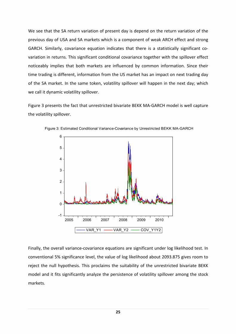
Figure 3 presents the fact that unrestricted bivariate BEKK MA-GARCH model is well capture

the volatility spillover.

Finally, the overall variance-covariance equations are significant under log likelihood test. In

conventional 5% significance level, the value of log likelihood about 2093.875 gives room to

reject the null hypothesis. This proclaims the suitability of the unrestricted bivariate BEKK

model and it fits significantly analyze the persistence of volatility spillover among the stock

markets.

-1

0

1

2

3

4

5

6

2005 2006 2007 2008 2009 2010

VAR_Y1 VAR_Y2 COV_Y1Y2

Figure 3: Estimated Conditional Variance-Covariance by Unrestricted BEKK MA-GARCH

26

6. Conclusion and Further Studies

The substantial increase in global capital flow along with the globalized economy is

attributed for the existence of interdependence between financial markets which is more

apparent than before. In the other side of the mirror, financial crisis was frequently

happened and adversely affect the global economy. This thesis investigates weather there is

stock market co-movement and volatility spillover between the USA and South Africa

markets. I employed daily stock return indices from Apr 1, 2005 to May 31, 2011.

First, by applying VAR representation approach based on two lag period, I found evidence of

uni-directional return spillover, which is from the NYSE to JSE. In this circumstance,

information from the US market has made impact on the SA market. According to the

assessment of trading time of both markets, the South Africa market is strongly affected on

what happened in the US market one period lag stock movement. Finally, the unrestricted

bivariate MA-GARCH – BEKK model is built to capture the existence of volatility spillover

between returns of the NYSE and JSE stock indices. I found significant own past shocks and

past volatility persistence impact on the current return fluctuation of both markets. Though

the dynamics of the conditional volatilities differ, there is uni-directional volatility

transmission between these two markets. This is due to the existence of significant and

positive shocks and volatility spillovers from USA to SA. Based on this, I conclude that USA

has influential impact on the South Africa stock return movement.

In summary, I consider my result support the finding in established literature on stock return

co-movement and volatility spillover between developed and emerging markets. Hence,

stakeholders on the investment activity, including government, should pay attention on the

behavior of volatility transmission. Policy makers and private as well as institutional

investors should modify their investment strategy and asset allocation decisions accordingly

to the spillover effects so that they can protect their investment from default and/or make

profit by hedging their investment.

Last but not least, however, this thesis could also be improved in the following ways. Firstly,

beside USA, one strong European market could be included to examine the effect from which

South Africa is strongly affected. Secondly, the study can be done by dividing the sample in to

two sub-samples: pre-reformation and post-reformation of South African market.

27

Reference

"Eviews 6 User Guide II."

Balios. D & Xanthakis. M 2003, "International Interdependence and Daynamic Linkages Between

Developed Stock Markets", South Eastern EuropeJournal of Economics 1, pp. 105-130

viewed May 02, 2011,

http://www.asecu.gr/Seeje/issue01/baliosxanthakis.pdf.

Beirne. J, Maria Caporale G, Schulze-Ghattas. M & Spagnolo. N 2008, "Volatility Spillovers and

Contagion from Mature to Emerging Stock Markets", Working Paper WP/08/286,

IMF, viewed Apr 13, 2011,

http://www.imf.org/external/pubs/ft/wp/2008/wp08286.pdf.

Bollerslev. T 1986, "Generalized autoregresive conditional heteroskedasticity",

Journal of Econometrics, vol. 31. (1986), pp 307-327.

Bollerslev. T 1987, "A conditionally Hetroskedastic Time Series Model for Speculative Prices

and Rates of Return", The Review of Economic and Statistics, Vol.69, No.3 (Aug 1987), pp542-547.

Bollerslev.T, Andersen. T 1997, "Interday Periodicity and Volatility Persistence in Financial Markets",

Journal of Empirical Finance, No.4 (1997), pp 115-158.

Bordo M. D 2000, "International Financial Markets: The Chalenge of Globalization", NBER,

viwed Mar 29, 2011, http://econweb.rutgers.edu/bordo/global.pdf.

Carmona. R 2004, Statistical Anaysis of Financial Data in S-Plus, Springer, USA.

Cont R. 2000. "Empirical Properties of Asset Returns: Stylized Facts and Statistical Issues",

Quantitative Finance, Vol. 1, PP. 223-236, viewed Apr 13, 2011,

http://citeseer.ist.psu.edu/viewdoc/download;jsessionid...?doi=10.1.1.16.5992.pdf.

Dymski. G 2005, "Financial Globalization, Social Exclusion and Financial Crisis",

International Review of Applied Economics, Vol. 19, No. 4, 439–457, viewed May 05, 2011,

http://www.econ.uoa.gr/UA/files/353039075..pdf.

Engle. F 1982, "Autoregeresive Conditional Heteroscedasticity withEstimates of the

Variance of UK Infilation", Econometrica, Vol. 50, No.4. (1982), pp.987-1008

viewed Mar 21, 2011, http://finance.martinsewell.com/arch-garch/Engle1982.pdf.

Engle. F and Kroner. F 1995, "Multivariate Simultaneous Generalized Arch",

Econometrica, Vol. 11, No. 1. pp. 122-150, viwed Mar 18,2011,

http://harrisd.net/papers/ARCHSV/Multivariate%20ARCH/EngleKroner1995ET.pdf.

Frankel. J 1994, "Price Volatility and Volume Spillovers between the Tokyo and

New York Stock Markets", The Internationalization of Equity Markets, University of

Chicago Press, pp309-343, viewed Mar 15, 2011, http://www.nber.org/chapters/c6277.

28

Gourieroux. C & Monfort. A 1997, Time Series and Dynamic Models, Bell and Bain Ltd., Glasgow.

Greene W. H, 2008. Econometric Analysis, 6th edn,Person Education, New Jersey.

Isard. P 2005, "Globalization and the International Financial System", Cambridge University Press, USA.

Jefferis. K, Smith. G 2005, "The Changing Effeiciency of African Stock Markets",

South African Journal of Economics, Vol. 73:1, pp54-67.

Jones. P 2002, Invesyments: Analysis and Management, 7th edn, John Wiley & Sons, Inc, USA.

Karanasos. M, Kim. J 2005, "The Inflation-Output Variability Relationship in the G3: A Bivariate

GARCH (BEKK) Approach", Risk Letters, 1 (2), 17-22, viewed May 19, 2011,

http://www.mkaranasos.com/RL05.pdf.

Karolyi. A 1995, "A Multivariate GARCH Model of International Transmissions of Stock Returns

and Volatility: The Case of the United States and Canada",

Journal of Business & Economic Statistics, Vol. 13, No. 1, pp. 11-25, viewed May 05, 2011,

http://harrisd.net/papers/ARCHSV/Multivariate%20ARCH/Karolyi1995JBES.pdf.

Kim. S & Rogers. H 1995, "International Stock Price Spillovers and Market Liberalization:

Evidence from Korea, Japan and the United States", BGFRS International Finance

Discussion Papers, No. 499, viwed May 02, 2011,

http://www.federalreserve.gov/pubs/IFDP/1995/499/ifdp499.pdf.

Liao. A &Williams. J 2004, "Volatility Transmssion and Changes in Stock Market Interdependence

in the European Community", European Review of Economics and Finance, Vol. 3, No. 3,

PP.203-231, viwed Mar 15, 2011, http://eprints.mdx.ac.uk/4068/1/Liao_Wms04_EREF.pdf.

Liu. Y & Pan Ming–Shiun 1997 "Mean and Volatility Spillover Effects in the U.S. And

Pacific–Basin Stock Markets", Multinational Finance Journal, 1997, vol. 1, no. 1, pp. 47–62

viwed May 02, 2011, http://mfs.rutgers.edu/mfj/Articles-pdf/V01N1p3.pdf

http://mfs.rutgers.edu/mfj/Articles-pdf/V01N1p3.pdf.

Martens. M 2001, "Forecasting daily exchange rate volatility using intraday returns",

Journal of International Money and Finance, No.20, PP.1-23, viwed May 03, 2011

http://wwwdocs.fce.unsw.edu.au/economics/Research/

Time%20Series%20and%20Applied%20Macroeconomics%20Group/JIMF2001.pdf.

Martin. Surya M 2009, "Volatility spillover in Indonesia, USA, and Japan capital market",

MPRA Paper No. 16914, viewed Mar 14, 2011,

http://mpra.ub.uni-muenchen.de/16914/School Press, USA.

29

Mason. S P 1995, "The Global Financial System: The Allocation of Risk", Harvard Business

School Press, USA.

Mishkin. F S 2005, "IS FINANCIAL GLOBALIZATION BENEFICIAL?", Working Paper 11891,

viwed Apr 23, 2011,

http://www.nber.org/papers/w11891.

Mundell. R A 2000, "A Reconsideration of the Twentieth Century", The American Economic Review,

Vol. 90, No. 3, pp. 327-340, viewed Apr 30, 2011,

http://nobelprize.org/nobel_prizes/economics/laureates/1999/mundell-lecture.pdf.

Penza. P & Bansal. V K 2001, Measuring Market Risk With Value at Risk, John Wiley & Sons, Inc, USA.

Rashid Sabri. N 2002, "Increasing Linkages of Stock Market and Price Volatility", Financial Risk and

Financial Risk Management, Volume 16, pages 349–373, viewed Mar 14, 2011,

http://home.birzeit.edu/commerce/sabri/link.pdf.

Sariannidis. N, Konteos. G & Drimbetas. E 2010, "Volatility Linkages among India, Hong Kong

and Singapore Stock Markets", International Research Journal of Finance and Economics,

EuroJournals Publishing, viewed Mar 17, 2011, http://www.eurojournals.com/finance.htm.

Schmukler. S L 2004, "Financial Globalization: Gain and Pain for Developing Countries",

Federal Reserve Bank of Atlanta Economic Review, viewed May 03, 2011,

http://www.frbatlanta.org/filelegacydocs/erq204_schmukler.pdf.

Shamiri. A & Isa. Z 2009, "The US Crisis and the Volatility Spillover Across South East

Asia Stock Markets ", International Research Journal of Finance and Economics,

ISSN 1450-2887, No. 34, pp. 8-17 viewed May 20, 2011, http://www.eurojournals.com/finance.htm.

Shutes. K & Niklewski. J 2010, "Multivariate GARCH Models - A Comparative Study of the Impact of

Alternative Methodologies on Correlation", Economics, Finance & Accounting Applied

Research Working Paper Series, viewed beginning of March 16, 2011,

http://wwwm.coventry.ac.uk/bes/cubs/aboutthebusinessschool/

Economicsfinanceandaccounting/Documents/RP2010-1.pdf.

Silvennoinen. A, Teräsvirta. T 2008, "Multivariate GARCH models", SSE/EFI Working Paper Series in

Economics and Finance No. 669, viewed Mar 16, 2011,

http://swopec.hhs.se/hastef/papers/hastef0669.pdf.

Singh. P, Kumar. B & Pandey. A 2008, "Price and Volatility Spillovers across North American,

European and Asian Stock Markets: With Special Focus on Indian Stock Market"

W.P. No.2008-12-04, INDIAN INSTITUTE OF MANAGEMENT viewed Apr 13, 2011

http://www.slideshare.net/Zorro29/price-and-volatility-spillovers-across-north-american.

30

Sok-Gee. C & Abd Karim 2010, "Volatility Spillovers of the Major Stock Markets in ASEAN-5

with the U.S. and Japanese Stock Markets",International Research Journal of

Finance and Economics, ISSN 1450-2887, No. 44, pp.157-168, viewed May 06, 2011,

http://www.eurojournals.com/finance.htm.

Soultanaeva. A 2011, "Back on the Map: Influence of News in Moscow and

New York on Returns and Risks of the Baltic State Stock Indices", Umeå University, Umeå.

Surya. M M 2009, Volatility Spillover in Indonesia, USA and Japan Capital Market, Munich Personal

RePEc Archive, viewed beginnig of March 2011, http://mpra.ub.uni-muenchen.de/16914/.

Tsay. S R 2005, "Analysis of Financial Time Series", 2nd edn, A John Wiley & Sons, Inc., Publication,

Canada.

Wang. M & Shih. F 2010, "VolatilityY Spillover: Ddynamic Rregional", European Journal

of Finance and Banking Research, Vol. 3. No. 3. 2010. pp 28-38 viewed Apr 14, 2011

http://www.globip.com/pdf_pages/european-vol3-article3.pdf.

Yu. J C 2005, "A Note on The Asymmetric Effect of Shocks on Market Return Volatility:

the Philippine Case", Philippine Management Review, Vol. 12, pp. 1-8, viewed Mar 14, 2011

http://journals.upd.edu.ph/index.php/pmr/article/viewFile/1826/1732.

31

Appendix

Table 1: Estimated parameters for the mean return model

Vector Autoregression Estimates

Date: 05/30/11 Time: 00:11

Sample (adjusted): 4/05/2005 3/31/2011

Included observations: 1563 after adjustments

Standard errors in ( ) & t-statistics in [ ]

DRNYSE DRJSE

DRNYSE(-1) -0.142600 0.381099

(0.02905) (0.02602)

[-4.90888] [ 14.6472]

DRNYSE(-2) -0.120938 0.074170

(0.03091) (0.02769)

[-3.91196] [ 2.67861]

DRJSE(-1) 0.075922 -0.172133

(0.03253) (0.02913)

[ 2.33405] [-5.90830]

DRJSE(-2) 0.019117 -0.040130

(0.02973) (0.02663)

[ 0.64309] [-1.50717]

C 0.003396 0.027731

(0.01663) (0.01489)

[ 0.20422] [ 1.86192]

R-squared 0.020914 0.123393

Adj. R-squared 0.018400 0.121143

Sum sq. resids 670.7431 538.0888

S.E. equation 0.656137 0.587683

F-statistic 8.319832 54.82702

Log likelihood -1556.671 -1384.457

Akaike AIC 1.998299 1.777936

Schwarz SC 2.015427 1.795065

Mean dependent 0.004542 0.024630

S.D. dependent 0.662258 0.626880

Determinant resid covariance (dof adj.) 0.110329

Determinant resid covariance 0.109624

Log likelihood -2707.942

Akaike information criterion 3.477852

Schwarz criterion 3.512109

32

Table A2: Estimated parameters for full BEKK MA-GARCH presentation

LogL: BVGARCH

Method: Maximum Likelihood (Marquardt)

Sample: 4/04/2005 3/31/2011

Included observations: 1564

Evaluation order: By observation

Estimation settings: tol= 1.0e-05, derivs=accurate numeric

Initial Values: MU(1)=0.15761, MU(2)=0.21396, TETA(1)=0.10000,

TETA(2)=0.10000, OMEGA(1)=0.05270, BETA(1)=0.50000,

BETA(3)=0.50000, ALPHA(1)=0.50000, ALPHA(3)=0.50000,

OMEGA(3)=0.07695, OMEGA(2)=0.00000, BETA(4)=0.50000,

BETA(2)=0.50000, ALPHA(4)=0.50000, ALPHA(2)=0.50000

Convergence achieved after 97 iterations Coefficient Std. Error z-Statistic Prob.

MU(1) 0.026945 0.008136 3.312081 0.0009

MU(2) 0.039351 0.011619 3.386832 0.0007

TETA(1) -0.243372 0.021930 -11.09786 0.0000

TETA(2) -0.011246 0.024343 -0.461993 0.6441

OMEGA(1) -0.049163 0.006274 -7.835631 0.0000

BETA(1) 0.958416 0.005025 190.7134 0.0000

BETA(3) 7.32E-05 0.011985 0.006108 0.9951

ALPHA(1) -0.295548 0.022820 -12.95111 0.0000

ALPHA(3) 0.043499 0.024240 1.794543 0.0727

OMEGA(3) 0.084485 0.014256 5.926251 0.0000

OMEGA(2) -0.062655 0.023220 -2.698270 0.0070

BETA(4) 0.899498 0.012098 74.34840 0.0000

BETA(2) 0.022000 0.008962 2.454783 0.0141

ALPHA(4) 0.383423 0.025239 15.19144 0.0000

ALPHA(2) -0.384320 0.027156 -14.15224 0.0000

Log likelihood -2093.875 Akaike info criterion 2.696771

Avg. log likelihood -1.338795 Schwarz criterion 2.748130

Number of Coefs. 15 Hannan-Quinn criter. 2.715864

33

Table A3: Estimated Parameters for MA (1)

MA Model Parameters

Estimate SE t Sig.

RNYSE-Model_1 RNYSE No Transformation Constant ,004 ,015 ,302 ,763

MA Lag 1 ,117 ,025 4,657 ,000

RJSE-Model_2 RJSE No Transformation Constant ,025 ,016 1,511 ,131

MA Lag 1 -,026 ,025 -1,022 ,307

Table A4: Correlations

RNYSE RJSE

RNYSE Pearson Correlation 1 ,430**

Sig. (2-tailed) ,000

N 1565 1565

RJSE Pearson Correlation ,430**

1

Sig. (2-tailed) ,000

N 1565 1565

**. Correlation is significant at the 0.01 level (2-tailed).

34

Figure A1: Stock indices

35

Figure 2A: Frequency distribution of NYSE and JSE daily return series

36

Figure 3A: Estimated Conditional Variance of NYSE and JSE by Full BEKK Model

0

1

2

3

4

5

6

2005 2006 2007 2008 2009 2010

VAR_NYSE

0

1

2

3

4

5

6

2005 2006 2007 2008 2009 2010

VAR_JSE

37

Unrestricted Version of bi-variate MA-GARCH BEKK

PRG (28/12/2011)

BV_MA_GARCH.PRG (02/21/2012) ' unrestricted version of ' bi-variate BEKK of Engle and Kroner (1995): ' ' y = µ + res ' µ= c+Θres(-1) ' res ~ N(0,H) ' ' H = omega*omega' + beta H(-1) beta' + alpha res(-1) res(-1)' alpha' ' ' where ' ' y = 2 x 1 ' µ = 2 x 1 ' H = 2 x 2 (symmetric) ' H(1,1) = variance of y1 (saved as var_y1) ' H(1,2) = cov of y1 and y2 (saved as var_y2) ' H(2,2) = variance of y2 (saved as cov_y1y2) ' omega = 2 x 2 low triangular ' beta = 2 x 2 ' alpha = 2 x 2 ' 'change path to program path %path = @runpath cd %path load nysejse.wf1 ' dependent variables of both series must be continues smpl @all series y1 = DRNYSE series y2 = DRJSE ' set sample ' first observation of s1 need to be one or two periods after ' the first observation of s0 sample s0 4/1/2005 3/31/2011 sample s1 4/2/2005 3/31/2011 ' initialization of parameters and starting values ' change below only to change the specification of model smpl s0 'get starting values from univariate GARCH equation eq1.arch(m=100,c=1e-5) y1 c ma(1) equation eq2.arch(m=100,c=1e-5) y2 c ma(1) ' declare coef vectors to use in bi-variate GARCH model ' see above for details coef(2) mu mu(1)= eq1.c(1)^.5 mu(2)= eq2.c(1)^.5 coef(3) teta teta(1) = .1 teta(2)= .1 coef(4) omega omega(1)=eq1.c(3)^.5 omega(2)=0

38

omega(3)=eq2.c(3)^.5 coef(5) alpha alpha(1) = 0.5 alpha(2) = 0.5 alpha(3) = 0.5 alpha(4) = 0.5 coef(5) beta beta(1)= 0.5 beta(2)= 0.5 beta(3) =0.5 beta(4)= 0.5 ' constant adjustment for log likelihood !mlog2pi = 2*log(2*@acos(-1)) ' use var-cov of sample in "s1" as starting value of variance-covariance matrix series cov_y1y2 = @cov(y1-mu(1), y2-mu(2)) series var_y1 = @var(y1) series var_y2 = @var(y2) series sqres1 = (y1-mu(1))^2 series sqres2 = (y2-mu(2))^2 series res1res2 = (y1-mu(1))*(y2-mu(2)) smpl 4/1/2005 4/2/2005 series res1=y1-mu(1) series res2=y2-mu(2) smpl 4/2/2005 3/31/2011 series res1=y1-mu(1)-teta(1)*res1(-1) series res2=y2-mu(2)-teta(2)*res2(-1) series cov_y1y2 = @cov(y1-mu(1)-teta(1)*res1(-1), y2-mu(2)-teta(2)*res2(-1)) series var_y1 = @var(y1-teta(1)*res1(-1)) series var_y2 = @var(y2-teta(2)*res2(-1)) series sqres1=y1-mu(1)-teta(1)*res1(-1)^2 series sqres2=y2-mu(2)-teta(2)*res2(-1)^2 series res1res2=(y1-mu(1)-teta(1)*res1(-1))*(y2-mu(2)-teta(2)*res2(-1)) ' ........................................................... ' LOG LIKELIHOOD ' set up the likelihood ' 1) open a new blank likelihood object (L.O.) name bvgarch ' 2) specify the log likelihood model by append ' ........................................................... logl bvgarch bvgarch.append @logl logl smpl 4/1/2005 4/2/2005 bvgarch.append res1=y1-mu(1) bvgarch.append res2=y2-mu(2)

39

smpl 4/1/2005 4/2/2005 bvgarch.append sqres1=(y1-mu(1))^2 bvgarch.append sqres2=(y2-mu(2))^2 bvgarch.append res1res2= (y1-mu(1))*(y2-mu(2)) smpl 4/2/2005 3/31/2011 bvgarch.append res1=y1-mu(1)-teta(1)*res1(-1) bvgarch.append res2=y2-mu(2)-teta(2)*res2(-1) smpl 4/2/2005 3/31/2011 bvgarch.append sqres1 = (y1-mu(1)-teta(1)*res1(-1))^2 bvgarch.append sqres2 = (y2-mu(2)-teta(2)*res2(-1))^2 bvgarch.append res1res2 = (y1-mu(1)-teta(1)*res1(-1))*(y2-mu(2)-teta(2)*res2(-1)) ' calculate the variance and covariance series bvgarch.append var_y1 = omega(1)^2 + beta(1)^2*var_y1(-1)+beta(1)*beta(3)*cov_y1y2(-1)+beta(1)*beta(3)*cov_y1y2(-1)+beta(3)^2*var_y2(-1) + alpha(1)^2*sqres1(-1)+alpha(1)*alpha(3)*res1res2(-1)+alpha(1)*alpha(3)*res1res2(-1)+alpha(3)^2*sqres2(-1) bvgarch.append var_y2 = omega(3)^2+omega(2)^2 +beta(4)^2*var_y2(-1)+beta(4)*beta(2)*cov_y1y2(-1)+beta(4)*beta(2)*cov_y1y2(-1)+beta(2)^2*var_y1(-1) + alpha(4)^2*sqres2(-1)+alpha(4)*alpha(2)*res1res2(-1)+alpha(4)*alpha(2)*res1res2(-1)+alpha(2)^2*sqres1(-1) bvgarch.append cov_y1y2 = omega(1)*omega(2) + beta(2)^2*var_y1(-1) + beta(3)*beta(2)*cov_y1y2(-1) + beta(1)*beta(4)*cov_y1y2(-1) + beta(4)*beta(3)*var_y2(-1) + alpha(2)*alpha(1)*sqres1(-1) + alpha(4)*alpha(1)*res1res2(-1) + alpha(3)*alpha(2)*res1res2(-1) + alpha(4)*alpha(3)*sqres2(-1) ' determinant of the variance-covariance matrix bvgarch.append deth = var_y1*var_y2 - cov_y1y2^2 ' inverse elements of the variance-covariance matrix bvgarch.append invh1 = var_y2/deth bvgarch.append invh3 = var_y1/deth bvgarch.append invh2 = -cov_y1y2/deth ' log-likelihood series bvgarch.append logl =-0.5*(!mlog2pi + (invh1*sqres1+2*invh2*res1res2+invh3*sqres2) + log(deth)) ' remove some of the intermediary series ' bvgarch.append @temp invh1 invh2 invh3 sqres1 sqres2 res1res2 deth ' estimate the model smpl s1 bvgarch.ml(showopts, m=100, c=1e-5) ' change below to display different output show bvgarch.output graph varcov.line var_y1 var_y2 cov_y1y2 show varcov ' LR statistic for univariate versus bivariate model scalar lr = -2*( eq1.@logl + eq2.@logl - bvgarch.@logl ) scalar lr_pval = 1 - @cchisq(lr,1)