stochasticdynamicsystemswithcomplex …user.engineering.uiowa.edu/~rahman/ijnme_comrep.pdfoperators...

INTERNATIONAL JOURNAL FOR NUMERICAL METHODS IN ENGINEERINGInt. J. Numer. Meth. Engng 2007; 71:963–986Published online 5 January 2007 in Wiley InterScience (www.interscience.wiley.com). DOI: 10.1002/nme.1973

Stochastic dynamic systems with complex-valued eigensolutions

Sharif Rahman∗,†,‡

Department of Mechanical & Industrial Engineering, The University of Iowa, Iowa City, IA 52242, U.S.A.

SUMMARY

A dimensional decomposition method is presented for calculating the probabilistic characteristics ofcomplex-valued eigenvalues and eigenvectors of linear, stochastic, dynamic systems. The methodinvolves a function decomposition allowing lower-dimensional approximations of eigensolutions,Lagrange interpolation of lower-dimensional component functions, and Monte Carlo simulation. Comparedwith the commonly used perturbation method, neither the assumption of small input variability nor thecalculation of the derivatives of eigensolutions is required by the method developed. Results of numericalexamples from linear stochastic dynamics indicate that the decomposition method provides excellentestimates of the moments and/or probability densities of eigenvalues and eigenvectors for various casesincluding large statistical variations of input. Copyright q 2007 John Wiley & Sons, Ltd.

Received 20 July 2006; Revised 21 November 2006; Accepted 22 November 2006

KEY WORDS: complex eigenvalue; random eigenvalue; random matrix; decomposition method; univariatedecomposition; bivariate decomposition; disc brake system

1. INTRODUCTION

Mathematical modelling and simulation to characterize dynamic systems and forecast theirevolution in time often lead to large-scale linear or non-linear eigenvalue problems. Generally,the coefficient matrices or operators in these eigenvalue problems are not precisely known be-cause of insufficient information, limited understanding of the underlying phenomena, and inherentrandomness. Eigenvalue problems defined for such random matrix, differential, or integraloperators are referred to as random eigenvalue problems and are commonly solved by stochastic

∗Correspondence to: Sharif Rahman, Department of Mechanical & Industrial Engineering, The University of Iowa,Iowa City, IA 52242, U.S.A.

†E-mail: [email protected], Website: http://www.engineering.uiowa.edu/∼rahman‡Professor.

Contract/grant sponsor: U.S. National Science Foundation; contract/grant number: DMI-0355487

Copyright q 2007 John Wiley & Sons, Ltd.

964 S. RAHMAN

methods that determine statistical moments, probability law, and other relevant properties ofeigensolutions.

Over the years, many approximate stochastic methods have been developed or examined forsolving random eigenvalue problems associated with undamped or proportionally damped stochas-tic systems. Of these methods, the perturbation methods have dominated the current literature [1–3]because of their ease of implementation and computational efficiency. However, these methodshave two major limitations: both the uncertainty of random input and the non-linearity of therandom eigenvalue or eigenvector with respect to random input must be small. Methods other thanthe perturbation methods include the iteration method [1], the Ritz method [4], the crossing theory[5], the stochastic reduced basis [6], the asymptotic method [7], the polynomial chaos expansion[8], and the recently developed dimensional decomposition method [9]. However, most if not all,of these past studies focus strictly on undamped or proportionally damped systems. Althoughconditions for proportional damping were derived by Caughey and O’Kelly [10], proportionaldamping is a mathematical construct that allows invoking classical normal modes. If the dampingis not proportional, as identified from practical modal testing, linear systems may possess com-plex modes instead of classical real modes. Complex modes may also appear for undamped orproportionally damped systems with unsymmetric stiffness matrices, for example, when there arefrictional springs. However, the consideration of complex modes in stochastic systems has not beenwidespread. Only recently have non-proportionally damped stochastic systems been examined; in2004, Adhikari employed the first-order perturbation method to derive the second-moment statis-tics of complex mode shapes and natural frequencies of simple dynamic systems [11]. However,the perturbation methods require expensive calculation of derivatives of eigensolutions, and moreimportantly, are limited to small non-linearity of input–output mapping or small input uncertainties.Hence, new stochastic methods for characterizing complex-valued eigensolutions that can managearbitrarily large non-linearity of input–output mapping and arbitrarily large uncertainties of inputare highly desirable.

This paper presents a dimensional decomposition method for predicting the statistical momentsand probability density functions of complex-valued eigensolutions of linear stochastic systems.The method can be viewed as an extension of the author’s previously developed dimensionaldecomposition method for analysing stochastic systems with real modes [9]. Section 2 formallydefines the random eigenvalue problem involving matrix operators. Section 3 gives a brief expositionof a function decomposition that facilitates lower-dimensional approximations of real and imaginaryparts of complex eigensolutions. Section 4 describes the proposed decomposition method andthe associated computational effort for calculating the probabilistic characteristics of complexeigenvalues and eigenvectors. In Section 5, three numerical examples from structural dynamicsillustrate the method developed. Comparisons have been made with direct Monte Carlo simulationto evaluate the accuracy and computational efficiency of the new method. Finally, Section 6provides conclusions from this work.

2. RANDOM EIGENVALUE PROBLEM

Let (�,F, P) be a probability space, where � is the sample space, F is the �-algebra of subsetsof �, and P is the probability measure; RN and CN be N -dimensional real and complex vectorspaces, respectively; and RN×N be a set of all N × N , real-valued matrices. Defined on theprobability space endowed with the expectation operator E, consider a real-valued N -dimensional

Copyright q 2007 John Wiley & Sons, Ltd. Int. J. Numer. Meth. Engng 2007; 71:963–986DOI: 10.1002/nme

STOCHASTIC DYNAMIC SYSTEMS 965

random vector X={X1, . . . , XN }T ∈ RN with the mean vector lX ≡ E[X] ∈ RN , the covariancematrix RX ≡ E[(X − lX)(X − lX)T] ∈ RN×N , and the joint probability density function fX(x) :RN �→ R.

Consider a family of L × L , real-valued, random coefficient matrices A j (X) ∈ RL×L ; j =1, . . . , J (J>0) and a general non-linear function f . A non-trivial solution of

f (�(X);A1(X), . . . ,AJ (X))/(X)= 0 (1)

if it exists, defines the random eigenvalue �(X) ∈ R or C and the random eigenvector /(X) ∈ RL

or CL of a general non-linear eigenvalue problem. For example, in stochastic dynamics, theequation of motion describing the free vibration of a linear, L-degree-of-freedom, discretesystem is

M(X)y(t) + C(X)y(t) + K(X)y(t)= 0 (2)

where the coefficient matrices are the random mass matrix M(X) ∈ RL×L , the random dampingmatrix C(X) ∈ RL×L , and the random stiffness matrix K(X) ∈ RL×L ; y(t)∈ RL is a vector ofgeneralized co-ordinates; and t ∈ R+ is the time, yielding a quadratic eigenvalue problem

[�2(X)M(X) + �(X)C(X) + K(X)]/(X) = 0 (3)

The probabilistic characteristics of random matrices M(X), C(X), and K(X) can be derivedfrom the probability law of X. In the present work focused on stochastic dynamics, the fol-lowing assumptions were made for the properties of coefficient matrices: (1) M(X) is symmet-ric and positive semi-definite; (2) C(X) is not necessarily proportional, i.e. it may in generalnot be expressed by a linear combination of M(X) and K(X); and (3) K(X) is not neces-sarily symmetric. The matrix properties allowed by assumptions (2) and/or (3) may generatecomplex-valued eigensolutions, where complex random eigenvalues �(X)= �R(X) ± √−1�I (X)

and complex random eigenvectors /(X) =/R(X) ± √−1/I (X) occur in conjugate pairs, andsubscripts R and I denote their real and imaginary parts, respectively. Both real and imaginaryparts of eigensolutions depend on the random input X via solution of the matrix characteristicequation

det[�2(X)M(X) + �(X)C(X) + K(X)] = 0 (4)

and subsequent solution of Equation (3). A major objective in solving a complex-valued ran-dom eigenvalue problem is to find the probabilistic characteristics of eigenpairs {�(i)

R (X) ±√−1�(i)I (X),/(i)

R (X) ± √−1/(i)I (X)}; i = 1, . . . , L when the probability law of X is arbitrarily

prescribed.

3. MULTIVARIATE FUNCTION DECOMPOSITION

Consider the real or imaginary part �m(x) : RN �→ R of a complex eigenvalue and the real or imag-inary part /m(x) : RN �→ RL of a complex eigenvector that depends on x={x1, . . . , xN }T ∈ RN ,where subscript m = R (real) or I (imaginary). A dimensional decomposition of �m(x) and /m(x),


966 S. RAHMAN

described by [12–20]

�m(x) = �m,0 +N∑i=1

�m,i (xi )︸︷︷︸=�m,1(x)

+N∑

i1,i2=1i1<i2

�m,i1i2(xi1, xi2)

︸︷︷︸=�m,2(x)

+ · · · +N∑

i1,...,iS=1i1<···<iS

�m,i1···iS (xi1, . . . , xiS )

︸︷︷︸=�m,S(x)

+ · · · + �m,12···N (x1, . . . , xN ) (5)

and

/m(x) =/m,0 +N∑i=1/m,i (xi )︸︷︷︸

=/m,1(x)

+N∑

i1,i2=1i1<i2

/m,i1i2(xi1, xi2)

︸︷︷︸=/m,2(x)

+ · · · +N∑

i1,...,iS=1i1<···<iS

/m,i1···iS (xi1, . . . , xiS )

︸︷︷︸=/m,S(x)

+ · · · + /m,12···N (x1, . . . , xN ) (6)

can be viewed as a finite hierarchical expansion of an output function in terms of its input variableswith increasing dimensions, where �m,0 and /m,0 are constants; �m,i (xi ) : R �→ R and /m,i (xi ) :R �→ RL are univariate component functions representing individual contribution to �m(x) and/m(x) by input variable xi acting alone; �m,i1i2(xi1, xi2) : R2 �→ R and /m,i1i2(xi1, xi2) : R2 �→ RL

are bivariate component functions describing the cooperative influence of two input variablesxi1 and xi2 ; �m,i1···iS (xi1, . . . , xiS ) : RS �→ R and /m,i1···iS (xi1, . . . , xiS ) : RS �→ RL are S-variatecomponent functions quantifying the cooperative effects of S input variables xi1, . . . , xiS ; and soon. If

�m,S(x)= �m,0 +N∑i=1

�m,i (xi ) +N∑

i1,i2=1i1<i2

�m,i1i2(xi1, xi2) + · · · +N∑

i1,...,iS=1i1<···<iS

�m,i1···iS (xi1, . . . , xiS ) (7)

and

/m,S(x)=/m,0+N∑i=1/m,i (xi )+

N∑i1,i2=1i1<i2

/m,i1i2(xi1, xi2)+ · · · +N∑

i1,...,iS=1i1<···<iS

/m,i1···iS (xi1, . . . , xiS ) (8)

represent general S-variate approximations of �m(x) and /m(x), respectively, the univariate (S = 1)approximations �m,1(x) and /m,1(x) and the bivariate (S = 2) approximations �m,2(x) and /m,2(x)provide two- and three-term approximants, respectively, of the finite decomposition in Equations (7)



and (8). Similarly, trivariate, quadrivariate, and other higher-variate approximations can be derivedby appropriately selecting the value of S. The fundamental conjecture underlying this work is thatcomponent functions arising in the eigenvalue function decomposition will exhibit insignificantS-variate effects cooperatively when S → N , leading to useful lower-variate approximations of�m(x) and /m(x). In the limit, when S = N , �m,S(x) and /m,S(x) converge to the exact functions�m(x) and /m(x), respectively. In other words, Equations (7) and (8) generate a hierarchical andconvergent sequence of approximations of eigensolutions.

The decomposition presented in Equations (5) or (6) can be traced to the work of Hoeffding[14] in the 1940s, and is well known in the statistics literature under the name analysis of variance(ANOVA) [15]. This decomposition, coined later as the high-dimensional model representation(HDMR) by Rabitz, has been further refined that led to notable contributions in function approxi-mation, including ANOVA-HDMR [16], cut-HDMR [17], and random-sampling (RS)-HDMR [18].Further generalizations to multi-cut HDMR [19] and monomial preconditioning (mp)-cut-HDMR[20] have also appeared. Recently, the author’s group exploited this decomposition techniquein calculating statistical moments of response [12] and reliability [13] of uncertain mechanicalsystems.

4. DIMENSIONAL DECOMPOSITION METHOD

4.1. Lower-dimensional approximations

For 1�S�N , consider S-variate approximations of �m(x) and /m(x), respectively, defined by

�m,S(x) ≡S∑

k=0(−1)k

(N − S + k − 1

k

)N∑

i1,...,iS−k=1i1<···<iS−k

�m(c1, . . . , ci1−1, xi1,

ci1+1, . . . , ciS−k−1, xiS−k , ciS−k+1, . . . , cN ) (9)

and

/m,S(x) ≡S∑

k=0(−1)k

(N − S + k − 1

k

)N∑

i1,...,iS−k=1i1<···<iS−k

/m(c1, . . . , ci1−1, xi1,

ci1+1, . . . , ciS−k−1, xiS−k , ciS−k+1, . . . , cN ) (10)

where c={c1, . . . , cN }T is a reference point, �m(c1, . . . , ci1−1, xi1, ci1+1, . . . , ciS−k−1, xiS−k ,

ciS−k+1, . . . , cN ) and /m(c1, . . . , ci1−1, xi1, ci1+1, . . . , ciS−k−1, xiS−k , ciS−k+1, . . . , cN ) are(S−k)th-dimensional component functions representing (S−k)th-dimensional cooperation amonginput variables xi1, . . . , xiS−k , where S = 1, . . . , N and k = 0, . . . , S. Based on the author’s pastexperience, the mean point of random input defines a suitable reference point. Using a multivariatefunction theorem developed by Xu and Rahman [12], it can be shown that �m,S(x) and /m,S(x)consist of all terms of the Taylor series of �m(x) and /m(x), respectively, that have less than orequal to S variables. The expanded form of Equation (9) or (10), when compared with the Taylor


968 S. RAHMAN

expansion of �m(x) or /m(x), indicates that the residual error in the S-variate approximationincludes terms of dimensions S+1 and higher. When S = 1 and 2, Equation (9) or (10) degeneratesto univariate or bivariate approximations, respectively. These univariate or bivariate approximations,which include all higher-order univariate or bivariate terms of �m(x) and /m(x), should thereforegenerally provide higher-order representations of eigenvalues than those provided by commonlyemployed first- or second-order perturbation methods.

The S-variate approximation described by Equations (9) or (10), when expanded and furthersimplified, can be shown to be equivalent to a cut-HDMR. However, if the input is random, theassociated component functions are also random. Therefore, further approximation of various com-ponent functions in the S-variate approximation or cut-HDMR is required for efficient stochasticcomputation, described as follows.

4.2. Lagrange interpolation

Consider (S − k)-variate component functions �m(c1, . . . , ci1−1, xi1, ci1+1, . . . , ciS−k−1, xiS−k ,

ciS−k+1, . . . , cN ) and/m(c1, . . . , ci1−1, xi1, ci1+1, . . . , ciS−k−1, xiS−k , ciS−k+1, . . . , cN ) in Equations

(9) and (10), respectively. If for sample points xi1 = x ( j1)i1

, . . . , xiS−k = x ( jS−k)

iS−k, nS−k function values

�m(c1, . . . , ci1−1, x( j1)i1

, ci1+1, . . . , ciS−k−1, x( jS−k)

iS−k, ciS−k+1, . . . , cN ); j1, jS−k = 1, . . . , n and nS−k

function values /m(c1, . . . , ci1−1, x( j1)i1

, ci1+1, . . . , ciS−k−1, x( jS−k)

iS−k, ciS−k+1, . . . , cN ); j1, jS−k =

1, . . . , n are numerically evaluated, the function values for an arbitrary point (xi1, . . . , xiS−k )

can be interpolated by

�m(c1, . . . , ci1−1, xi1, ci1+1, . . . , ciS−k−1, xiS−k , ciS−k+1, . . . , cN )

=n∑

jS−k=1· · ·

n∑j1=1

� j1(xi1) · · · � jS−k(xiS−k )�m(c1, . . . , ci1−1, x

( j1)i1

,

ci1+1, . . . , ciS−k−1, x( jS−k)

iS−k, ciS−k+1, . . . , cN ) (11)

and

/m(c1, . . . , ci1−1, xi1, ci1+1, . . . , ciS−k−1, xiS−k , ciS−k+1, . . . , cN )

=n∑

jS−k=1· · ·

n∑j1=1

� j1(xi1) · · · � jS−k(xiS−k )/m(c1, . . . , ci1−1, x

( j1)i1

,

ci1+1, . . . , ciS−k−1, x( jS−k)

iS−k, ciS−k+1, . . . , cN ) (12)

where

� j (xi ) =∏n

l=1,l �= j (xi − x (l)i )∏n

l=1,l �= j (x( j)i − x (l)

i )(13)



is the n-point Lagrange shape function. The combination of Equations (9)–(13) leads to generalS-variate approximations of eigensolutions, given by

�m,S(X) ∼=S∑

k=0(−1)k

(N − S + k − 1

k

)N∑

i1,...,iS−k=1i1<···<iS−k

n∑jS−k=1

· · ·n∑

j1=1� j1(Xi1) · · · � jS−k

(XiS−k )

×�m(c1, . . . , ci1−1, x( j1)i1

, ci1+1, . . . , ciS−k−1, x( jS−k)

iS−k, ciS−k+1, . . . , cN ) (14)

and

/m,S(X) ∼=S∑

k=0(−1)k

(N − S + k − 1

k

)N∑

i1,...,iS−k=1i1<···<iS−k

n∑jS−k=1

· · ·n∑

j1=1� j1(Xi1) · · · � jS−k

(XiS−k )

×/m(c1, . . . , ci1−1, x( j1)i1

, ci1+1, . . . , ciS−k−1, x( jS−k)

iS−k, ciS−k+1, . . . , cN ) (15)

which can be employed to generate a convergent sequence of lower-variate approximations of�m(X) or /m(X). For example, when S = 1, the univariate approximations are

�m,1(X) ∼=N∑i=1

n∑j=1

� j (Xi )�m(c1, . . . , ci−1, x( j)i , ci+1, . . . , cN ) − (N − 1)�m(c) (16)

and

/m,1(X) ∼=N∑i=1

n∑j=1

� j (Xi )/m(c1, . . . , ci−1, x( j)i , ci+1, . . . , cN ) − (N − 1)/m(c) (17)

whereas the selection of S = 2 yields the bivariate approximations

�m,2(X) ∼=N∑

i1,i2=1i1<i2

n∑j2=1

n∑j1=1

� j1(Xi1)� j2(Xi2)

× �m(c1, . . . , ci1−1, x( j1)i1

, ci1+1, . . . , ci2−1, x( j2)i2

, ci2+1, . . . , cN )

− (N − 2)N∑i=1

n∑j=1

� j (Xi )�m(c1, . . . , ci−1, x( j)i , ci+1, . . . , cN )

+ (N − 1)(N − 2)

2�m(c) (18)

and

/m,2(X) ∼=N∑

i1,i2=1i1<i2

n∑j2=1

n∑j1=1

� j1(Xi1)� j2(Xi2)


970 S. RAHMAN

×/m(c1, . . . , ci1−1, x( j1)i1

, ci1+1, . . . , ci2−1, x( j2)i2

, ci2+1, . . . , cN )

−(N − 2)N∑i=1

n∑j=1

� j (Xi )/m(c1, . . . , ci−1, x( j)i , ci+1, . . . , cN )

+ (N − 1)(N − 2)

2/m(c) (19)

Trivariate and other higher-variate approximations can be generated in a similar manner, but dueto their higher cost, only univariate and bivariate approximations are considered in this paper.

The sample points required by Lagrange interpolations can be selected based on the mean andstandard deviation of the random input. For example, if n sample points are uniformly deployedin the direction of Xi , which has mean �i and standard deviation �i , the sample points for theunivariate approximation are: (. . . , �i − 2�i , �i − �i , �i , �i + �i , �i + 2�i , . . .). Other selectionsentailing a sparser uniform spacing or a non-uniform spacing can be envisioned. Nonetheless,the number and location of sample points should be selected in such a way that the resultingapproximation is insensitive to further refinement. From the author’s past experience, a uniformspacing with five sample points works well unless the input uncertainty or the non-linearity ofthe component function is overly large, in which case a larger number of sample points maybe required. The appropriateness of selected sample points will be numerically evaluated in aforthcoming section.

4.3. Monte Carlo simulation

Once the Lagrange shape functions � j1(xi1), . . . ,� jS−k(xiS−k ), eigenvalue coefficients �m(c1, . . . ,

ci1−1, x( j1)i1

, ci1+1, . . . , ciS−k−1, x( jS−k)

iS−k, ciS−k+1, . . . , cN ), and eigenvector coefficients /m(c1, . . . ,

ci1−1, x( j1)i1

, ci1+1, . . . , ciS−k−1, x( jS−k)

iS−k, ciS−k+1, . . . , cN ); S = 1, . . . , N ; k = 0, . . . , S; j1, jS−k = 1,

. . . , n, are generated, Equations (14)–(19) provide explicit approximations of random eigensolu-tions {�(i)

R (X) ± √−1�(i)I (X),/(i)

R (X) ± √−1/(i)I (X)}; i = 1, . . . , L , in terms of random input

X. Therefore, any probabilistic characteristic of eigensolutions, including their moments andprobability density functions, can be easily evaluated by performing Monte Carlo simulation onEquations (14)–(19). Since Equations (14)–(19) do not require solving additional matrix equations,the embedded Monte Carlo simulation can be efficiently conducted for any sample size. Further-more, statistical moments obtained from Equations (14)–(19) can be employed in reconstructingprobability density function using the maximum entropy approach [21].

The proposed methods involving univariate (Equations (16) and (17)) or bivariate (Equations (18)and (19)) approximations, n-point Lagrange interpolation, and associated Monte Carlo simulationare defined as the univariate or bivariate decomposition methods in this paper. No expensivecalculation of partial derivatives of eigensolutions is required.

4.4. Computational effort

In reference to Equations (16) and (18), the univariate and bivariate decomposition methodsrequire evaluations of deterministic coefficients �m(c), �m(c1, . . . , ci−1, x

( j)i , ci+1, . . . , cN ), and

�m(c1, . . . , ci1−1, x( j1)i1

, ci1+1, . . . , ci2−1, x( j2)i2

, ci2+1, . . . , cN ) for m = R or I ; i, i1, i2 = 1, . . . , N ;



and j, j1, j2 = 1, . . . , n. Hence, the computational effort to obtain these coefficients can be viewedas numerically solving the associated deterministic characteristic equations

det[�2(c)M(c) + �(c)C(c) + K(c)]= 0 (20)

det[�2(c1, . . . , ci−1, x( j)i , ci+1, . . . , cN )M(c1, . . . , ci−1, x

( j)i , ci+1, . . . , cN )

+ �(c1, . . . , ci−1, x( j)i , ci+1, . . . , cN )C(c1, . . . , ci−1, x

( j)i , ci+1, . . . , cN )

+K(c1, . . . , ci−1, x( j)i , ci+1, . . . , cN )] = 0, i = 1, . . . , N , j = 1, . . . , n (21)

and

det[�2(c1, . . . , ci1−1, x( j1)i1

, ci1+1, . . . , ci2−1, x( j2)i2

, ci2+1, . . . , cN )

×M(c1, . . . , ci1−1, x( j1)i1

, ci1+1, . . . , ci2−1, x( j2)i2

, ci2+1, . . . , cN )

+ �(c1, . . . , ci1−1, x( j1)i1

, ci1+1, . . . , ci2−1, x( j2)i2

, ci2+1, . . . , cN )

×C(c1, . . . , ci1−1, x( j1)i1

, ci1+1, . . . , ci2−1, x( j2)i2

, ci2+1, . . . , cN )

+K(c1, . . . , ci1−1, x( j1)i1

, ci1+1, . . . , ci2−1, x( j2)i2

, ci2+1, . . . , cN )] = 0

i1, i2 = 1, . . . , N , j1, j2 = 1, . . . , n (22)

at several deterministic input defined by user-selected sample points. Therefore, the total costfor the univariate method entails a maximum of nN + 1 solutions of the matrix characteristicequation, and a maximum of N (N − 1)n2/2 + nN + 1 solutions of the matrix characteristicequation are required for the bivariate method. If the sample points include a common point in eachco-ordinate xi (see Example section), the numbers of such solutions reduce to (n − 1)N + 1 andN (N − 1)(n − 1)2/2 + (n − 1)N + 1 for the univariate and bivariate methods, respectively.Equations (9)–(22) are the result of a generalization of author’s previous work on real eigenvalue

problems [9]. Equations (9)–(22) will be employed in obtaining stochastic solutions of complex-valued eigenproblems in dynamic systems, including solving a large-scale eigenvalue problemfrom the automotive industry.

5. NUMERICAL EXAMPLES

Three numerical examples involving linear dynamics of a spring–mass–damper system, a cantileverbeam, and an automotive disc brake system are presented to illustrate the decomposition method.Comparisons have been made with the direct Monte Carlo simulation to evaluate the accuracy andefficiency of the proposed method. For the first two examples, the eigenvalues were calculated byan IMSL subroutine, which employs the state-space approach [22] and a hybrid double-shifted LR-QR algorithm [23]. A subspace projection algorithm embedded in the commercial finite elementcode ABAQUS (Version 6.5) [24] was employed to obtain eigenvalues for the third example.


972 S. RAHMAN

MK

C

KK

M MK

y1y2 y3

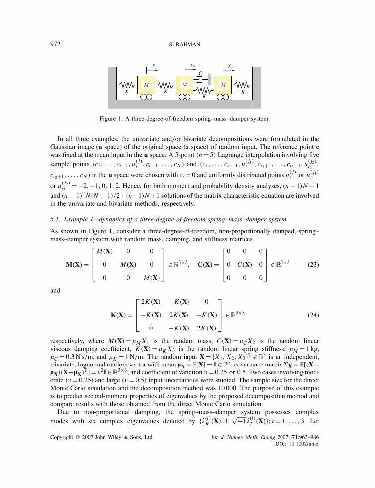
Figure 1. A three-degree-of-freedom spring–mass–damper system.

In all three examples, the univariate and/or bivariate decompositions were formulated in theGaussian image (u space) of the original space (x space) of random input. The reference point cwas fixed at the mean input in the u space. A 5-point (n = 5) Lagrange interpolation involving fivesample points (c1, . . . , ci−1, u

( j)i , ci+1, . . . , cN ) and (c1, . . . , ci1−1, u

( j1)i1

, ci1+1, . . . , ci2−1, u( j2)i2

,

ci2+1, . . . , cN ) in the u space were chosen with ci = 0 and uniformly distributed points u( j)i or u( j1)

i1

or u( j2)i2

= −2,−1, 0, 1, 2. Hence, for both moment and probability density analyses, (n− 1)N + 1

and (n − 1)2N (N − 1)/2+(n−1)N+1 solutions of the matrix characteristic equation are involvedin the univariate and bivariate methods, respectively.

5.1. Example 1—dynamics of a three-degree-of-freedom spring–mass–damper system

As shown in Figure 1, consider a three-degree-of-freedom, non-proportionally damped, spring–mass–damper system with random mass, damping, and stiffness matrices

M(X) =

⎡⎢⎢⎣M(X) 0 0

0 M(X) 0

0 0 M(X)

⎤⎥⎥⎦ ∈ R3×3, C(X) =

⎡⎢⎢⎣0 0 0

0 C(X) 0

0 0 0

⎤⎥⎥⎦ ∈ R3×3 (23)

and

K(X)=

⎡⎢⎢⎣2K (X) −K (X) 0

−K (X) 2K (X) −K (X)

0 −K (X) 2K (X)

⎤⎥⎥⎦ ∈ R3×3 (24)

respectively, where M(X)= �M X1 is the random mass, C(X) = �C X2 is the random linearviscous damping coefficient, K (X) = �K X3 is the random linear spring stiffness, �M = 1 kg,�C = 0.3N s/m, and �K = 1N/m. The random input X={X1, X2, X3}T ∈ R3 is an independent,trivariate, lognormal random vector with mean lX ≡ E[X] = 1∈ R3, covariance matrix RX ≡ E[(X−lX)(X−lX)T] = v2I∈ R3×3, and coefficient of variation v = 0.25 or 0.5. Two cases involving mod-erate (v = 0.25) and large (v = 0.5) input uncertainties were studied. The sample size for the directMonte Carlo simulation and the decomposition method was 10 000. The purpose of this exampleis to predict second-moment properties of eigenvalues by the proposed decomposition method andcompare results with those obtained from the direct Monte Carlo simulation.

Due to non-proportional damping, the spring–mass–damper system possesses complexmodes with six complex eigenvalues denoted by {�(i)

R (X) ± √−1�(i)I (X)}; i = 1, . . . , 3. Let



Y={�(1)R , �(2)

R , �(3)R , �(1)

I , �(2)I , �(3)

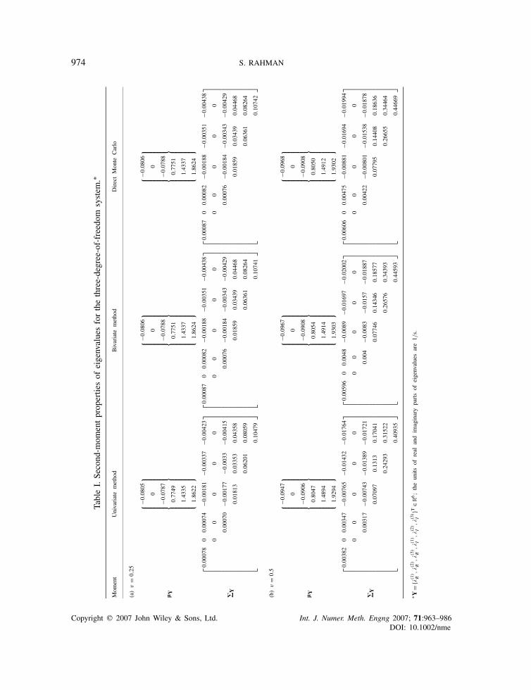
I }T ∈ R6 define a response vector comprising all three real and allthree imaginary parts of eigenvalues. Table I presents the mean vector (lY) and the covariancematrix (RY) of Y for both magnitudes of input uncertainties, calculated by the univariate andbivariate decomposition methods entailing only 13 and 61 solutions of the matrix characteristicequation, respectively. A direct Monte Carlo simulation by repeatedly solving the matrix character-istic equation was also performed to generate corresponding benchmark results, which are listed inTable I. The second rows of lY and RY contain zero elements, because the third and fourth eigen-values associated with the second mode are purely imaginary (i.e. �(2)

R (X) = 0). From the results ofTable I, the univariate and bivariate decomposition methods provide almost the same benchmarkestimates of means for both magnitudes of input uncertainties. When comparing covariance prop-erties for moderate input uncertainties (v = 0.25), the maximum errors in approximate variancesmeasured with respect to the direct Monte Carlo estimates are about 10% by the univariate methodand 0% by the bivariate method. The 0% error by the bivariate method is due to five significantdigits retained in comparing numerical values. Nonetheless, both versions of the decompositionmethod provide satisfactory estimates of the second-moment properties of eigenvalues for moderateinput uncertainties in this particular example. However, when there are large input uncertainties(v = 0.5), the maximum error by the univariate method rises to 37% and is no longer acceptable.In contrast, the bivariate method yields significantly improved results with errors less than 5%. Theerror can be further reduced by invoking a higher-variate decomposition method if desired. Thisimprovement is possible due to the hierarchical sequence of approximations in the dimensionaldecomposition method. Nevertheless, bivariate or higher-variate decomposition methods may berequired to account for large uncertainties of input. It is worth noting that the commonly employedperturbation methods are not expected to provide acceptable results for both magnitudes of inputuncertainties considered in this example [1–3]. An input coefficient of variation, as low as 10%,was required to yield satisfactory second-moment estimates of complex-valued eigensolutions byperturbation methods [11].

The statistics of Y predicted by the decomposition method were recalculated for a differentand new selection of sample points: u( j)

i or u( j1)i1

or u( j2)i2

= −3, −0.5, 0, 0.5, 3.§ The statisticsobtained using the new sample points are almost the same as listed in Table I. For example, themaximum difference in the variances calculated using new and old sample points by univariateor bivariate methods is only 0.3%. Such a comparison of results, although presented here for aspecific problem, shows that the final result is not so sensitive to the selection of sample points.

5.2. Example 2—flexural vibration of a free-standing beam

For the next example, the vibration of a tall, free-standing beam [22] shown in Figure 2(a) wasstudied. Figure 2(b) represents a lumped-parameter model of the beam, which comprises sevenrigid, massless links hinged together. The mass of the beam is represented by seven random pointmasses M located at the centre of each link. No damping was assumed except at the bottomjoint, where the random, rotational, viscous damping coefficient due to the foundation pad is C .The random rotational stiffness at the bottom of the beam, controlled by the lower half of thebottom link and the flexibility of the foundation pad, is K . The independent random variablesM , C , and K are lognormally distributed with respective means 3000 kg, 2× 107 Nm s/rad, and

§The new sample points, suggested by an anonymous reviewer, were used to evaluate the sensitivity of the method.


974 S. RAHMAN

TableI.Se

cond-m

omentpropertiesof

eigenvaluesforthethree-degree-of-freedom

system

.∗

Mom

ent

Univariatemethod

Bivariate

method

DirectMonte

Carlo

(a)

v=

0.25

l Y

⎧ ⎪ ⎪ ⎪ ⎪ ⎪ ⎪ ⎪ ⎪ ⎪ ⎨ ⎪ ⎪ ⎪ ⎪ ⎪ ⎪ ⎪ ⎪ ⎪ ⎩−0.080

5

0

−0.078

7

0.77

49

1.43

35

1.86

22

⎫ ⎪ ⎪ ⎪ ⎪ ⎪ ⎪ ⎪ ⎪ ⎪ ⎬ ⎪ ⎪ ⎪ ⎪ ⎪ ⎪ ⎪ ⎪ ⎪ ⎭

⎧ ⎪ ⎪ ⎪ ⎪ ⎪ ⎪ ⎪ ⎪ ⎪ ⎨ ⎪ ⎪ ⎪ ⎪ ⎪ ⎪ ⎪ ⎪ ⎪ ⎩−0.080

6

0

−0.078

8

0.77

51

1.43

37

1.86

24

⎫ ⎪ ⎪ ⎪ ⎪ ⎪ ⎪ ⎪ ⎪ ⎪ ⎬ ⎪ ⎪ ⎪ ⎪ ⎪ ⎪ ⎪ ⎪ ⎪ ⎭

⎧ ⎪ ⎪ ⎪ ⎪ ⎪ ⎪ ⎪ ⎪ ⎪ ⎨ ⎪ ⎪ ⎪ ⎪ ⎪ ⎪ ⎪ ⎪ ⎪ ⎩−0.080

6

0

−0.078

8

0.77

51

1.43

37

1.86

24

⎫ ⎪ ⎪ ⎪ ⎪ ⎪ ⎪ ⎪ ⎪ ⎪ ⎬ ⎪ ⎪ ⎪ ⎪ ⎪ ⎪ ⎪ ⎪ ⎪ ⎭

)Y

⎡ ⎢ ⎢ ⎢ ⎢ ⎢ ⎢ ⎢ ⎢ ⎢ ⎣0.00

078

00.00

074

−0.001

81−0

.003

37−0

.004

23

00

00

0

0.00

070

−0.001

77−0

.003

3−0

.004

15

0.01

813

0.03

353

0.04

358

0.06

201

0.08

059

0.10

479

⎤ ⎥ ⎥ ⎥ ⎥ ⎥ ⎥ ⎥ ⎥ ⎥ ⎦

⎡ ⎢ ⎢ ⎢ ⎢ ⎢ ⎢ ⎢ ⎢ ⎢ ⎣0.00

087

00.00

082

−0.001

88−0

.003

51−0

.004

38

00

00

0

0.00

076

−0.001

84−0

.003

43−0

.004

29

0.01

859

0.03

439

0.04

468

0.06

361

0.08

264

0.10

741

⎤ ⎥ ⎥ ⎥ ⎥ ⎥ ⎥ ⎥ ⎥ ⎥ ⎦

⎡ ⎢ ⎢ ⎢ ⎢ ⎢ ⎢ ⎢ ⎢ ⎢ ⎣0.00

087

00.00

082

−0.001

88−0

.003

51−0

.004

38

00

00

0

0.00

076

−0.001

84−0

.003

43−0

.004

29

0.01

859

0.03

439

0.04

468

0.06

361

0.08

264

0.10

742

⎤ ⎥ ⎥ ⎥ ⎥ ⎥ ⎥ ⎥ ⎥ ⎥ ⎦

(b)

v=

0.5

l Y

⎧ ⎪ ⎪ ⎪ ⎪ ⎪ ⎪ ⎪ ⎪ ⎪ ⎨ ⎪ ⎪ ⎪ ⎪ ⎪ ⎪ ⎪ ⎪ ⎪ ⎩−0.094

7

0

−0.090

6

0.80

47

1.48

94

1.92

94

⎫ ⎪ ⎪ ⎪ ⎪ ⎪ ⎪ ⎪ ⎪ ⎪ ⎬ ⎪ ⎪ ⎪ ⎪ ⎪ ⎪ ⎪ ⎪ ⎪ ⎭

⎧ ⎪ ⎪ ⎪ ⎪ ⎪ ⎪ ⎪ ⎪ ⎪ ⎨ ⎪ ⎪ ⎪ ⎪ ⎪ ⎪ ⎪ ⎪ ⎪ ⎩−0.096

7

0

−0.090

8

0.80

54

1.49

14

1.93

03

⎫ ⎪ ⎪ ⎪ ⎪ ⎪ ⎪ ⎪ ⎪ ⎪ ⎬ ⎪ ⎪ ⎪ ⎪ ⎪ ⎪ ⎪ ⎪ ⎪ ⎭

⎧ ⎪ ⎪ ⎪ ⎪ ⎪ ⎪ ⎪ ⎪ ⎪ ⎨ ⎪ ⎪ ⎪ ⎪ ⎪ ⎪ ⎪ ⎪ ⎪ ⎩−0.096

8

0

−0.090

8

0.80

50

1.49

12

1.93

02

⎫ ⎪ ⎪ ⎪ ⎪ ⎪ ⎪ ⎪ ⎪ ⎪ ⎬ ⎪ ⎪ ⎪ ⎪ ⎪ ⎪ ⎪ ⎪ ⎪ ⎭

)Y

⎡ ⎢ ⎢ ⎢ ⎢ ⎢ ⎢ ⎢ ⎢ ⎢ ⎣0.00

382

00.00

347

−0.007

65−0

.014

32−0

.017

64

00

00

0

0.00

317

−0.007

43−0

.013

89−0

.017

21

0.07

097

0.13

130.17

041

0.24

293

0.31

522

0.40

935

⎤ ⎥ ⎥ ⎥ ⎥ ⎥ ⎥ ⎥ ⎥ ⎥ ⎦

⎡ ⎢ ⎢ ⎢ ⎢ ⎢ ⎢ ⎢ ⎢ ⎢ ⎣0.00

596

00.00

48−0

.008

9−0

.016

97−0

.020

02

00

00

0

0.00

4−0

.008

3−0

.015

7−0

.018

87

0.07

746

0.14

346

0.18

577

0.26

576

0.34

393

0.44

593

⎤ ⎥ ⎥ ⎥ ⎥ ⎥ ⎥ ⎥ ⎥ ⎥ ⎦

⎡ ⎢ ⎢ ⎢ ⎢ ⎢ ⎢ ⎢ ⎢ ⎢ ⎣0.00

606

00.00

475

−0.008

81−0

.016

94−0

.019

94

00

00

0

0.00

422

−0.008

01−0

.015

38−0

.018

78

0.07

795

0.14

408

0.18

636

0.26

655

0.34

464

0.44

669

⎤ ⎥ ⎥ ⎥ ⎥ ⎥ ⎥ ⎥ ⎥ ⎥ ⎦

∗ Y=

{�(1)

R,�(2

)R

,�(3

)R

,�(1

)I

,�(2

)I

,�(3

)I

}T∈R

6;theunits

ofreal

and

imaginary

partsof

eigenvaluesare1/s.



l

l

l

l

l

l

x

l

y7

y6

y5

y4

y3

y2

y1

k 1

k 2

k 3

k 4

k 5

k 6

KC

M

M

M

M

M

M

M

M(ÿ2+ ÿ1)/2

M(ÿ3+ ÿ2)/2

M(ÿ4+ ÿ3)/2

M(ÿ5+ ÿ4)/2

M(ÿ6+ ÿ5)/2

M(ÿ7+ ÿ6)/2

Mÿ1/2

Mg

Mg

Mg

Mg

Mg

Mg

Mg(a) (b)

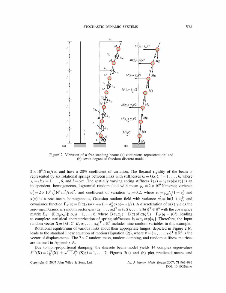
Figure 2. Vibration of a free-standing beam: (a) continuous representation; and(b) seven-degree-of-freedom discrete model.

2× 109 Nm/rad and have a 20% coefficient of variation. The flexural rigidity of the beam isrepresented by six rotational springs between links with stiffnesses ki ≡ k(xi ); i = 1, . . . , 6, wherexi = il; i = 1, . . . , 6, and l = 6m. The spatially varying spring stiffness k(x) = c� exp[�(x)] is anindependent, homogeneous, lognormal random field with mean �k = 2× 109 Nm/rad; variance

�2k = 2× 109v2k N2 m2/rad2; and coefficient of variation vk = 0.2; where c� = �k/

√1 + v2k and

�(x) is a zero-mean, homogeneous, Gaussian random field with variance �2� = ln(1 + v2k ) andcovariance function ��(u) ≡ E[�(x)�(x +u)] = �2� exp(−|u|/ l). A discretization of �(x) yields thezero-mean Gaussian random vector a≡{�1, . . . , �6}T ≡ {�(l), . . . , �(6l)}T ∈ R6 with the covariancematrix R� =[E(�p�q)]; p, q = 1, . . . , 6, where E(�p�q) = E(�(pl)�(ql))= ��((q − p)l), leadingto complete statistical characterization of spring stiffnesses ki = c� exp[�i ]. Therefore, the inputrandom vector X={M,C, K , �1, . . . , �6}T ∈ R9 includes nine random variables in this example.

Rotational equilibrium of various links about their appropriate hinges, depicted in Figure 2(b),leads to the standard linear equation of motion (Equation (2)), where y={y1, . . . , y7}T ∈ R7 is thevector of displacements. The 7× 7 random mass, random damping, and random stiffness matricesare defined in Appendix A.

Due to non-proportional damping, the discrete beam model yields 14 complex eigenvalues�(i)(X) = �(i)

R (X) ± √−1�(i)I (X); i = 1, . . . , 7. Figures 3(a) and (b) plot predicted means and


976 S. RAHMAN

1 2 3 4 5 6 7

Mode i

-120

-100

-80

-60

-40

-20

0

Mea

n of

λR

(i)

Monte Carlo

Univariate

Bivariate

1 2 3 4 5 6 7

Mode i

0

5

10

15

20

25

30

35

St.

dev.

of

λ R(i

)

Monte Carlo

Univariate

Bivariate

1 2 3 4 5 6 7

Mode i

0

1000

2000

3000

4000

5000

Mea

n of

λI(i

) , rad

/s

Monte Carlo

Univariate

Bivariate

1 2 3 4 5 6 7

Mode i

0

100

200

300

400

500

600

St. d

ev. o

f λ I(i

) , rad

/s

Monte Carlo

Univariate

Bivariate

(a)

(b)

Figure 3. Second-moment properties of eigenvalues of beam: (a) real part; and (b) imaginary part.

standard deviations of real parts �(i)R (X); i = 1, . . . , 7 and imaginary parts �(i)

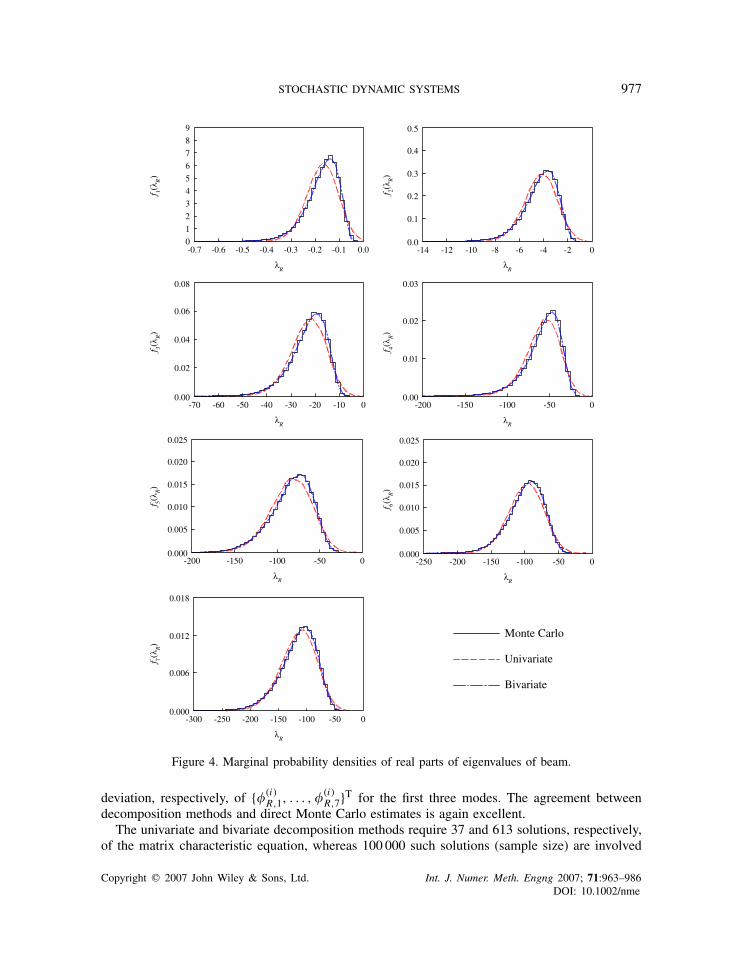
I (X); i = 1, . . . , 7,respectively, as a function of mode i , obtained by the univariate and bivariate decomposition meth-ods and the direct Monte Carlo simulation. The sample size for the direct Monte Carlo simulationand the decomposition method was 100 000. Compared with the direct Monte Carlo simulation,both versions of the decomposition method provide excellent estimates of second-moment prop-erties of eigenvalues. The marginal probability densities of seven real and seven imaginary partsof eigenvalues, respectively, plotted in Figures 4 and 5, also indicate a good agreement betweenresults from the decomposition and direct Monte Carlo methods. As expected, the bivariate methodis more accurate than the univariate method.

Corresponding to 14 eigenvalues, there are also 14 complex eigenvectors in conjugate pairs,denoted by /(i)(X) =/(i)

R (X) ± √−1/(i)I (X); i = 1, . . . , 7. Each eigenvector has 14 elements.

Consider the real part /(i)R (X)≡{�(i)

R,1, . . . ,�(i)R,7, �

(i)R,8, . . . , �

(i)R,14}T, where the first seven elements

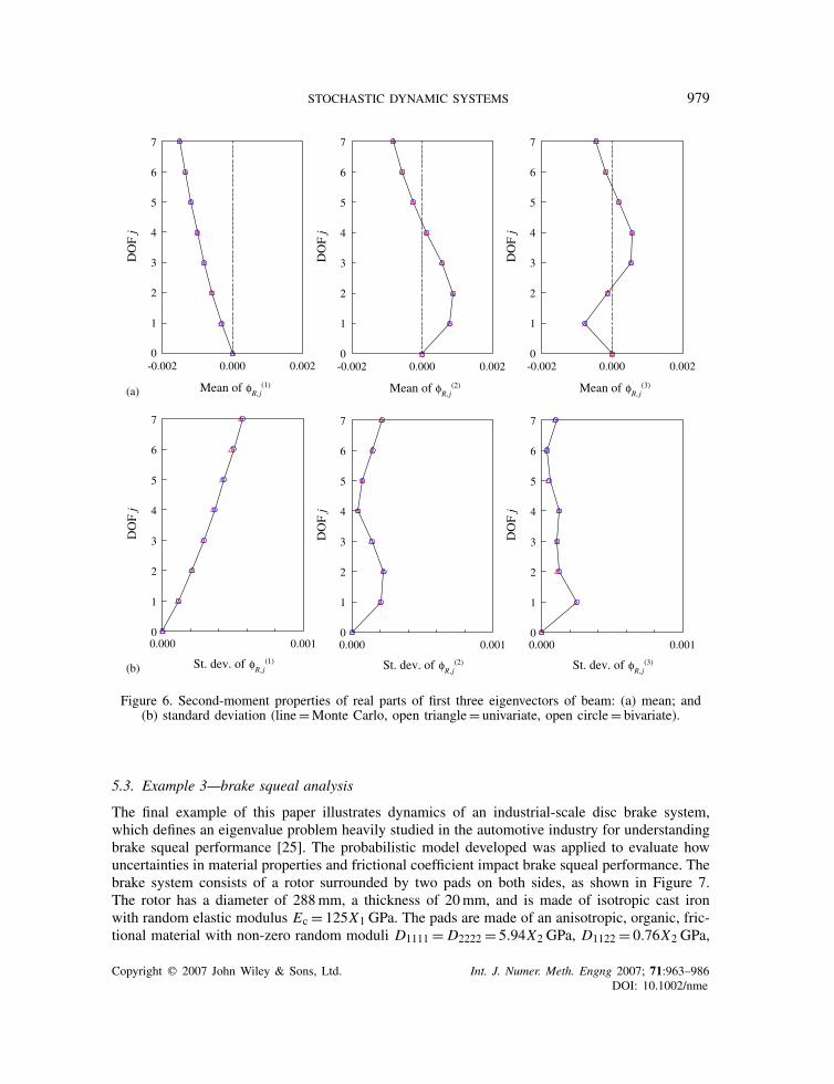
define the relative displacements of co-ordinates y1, . . . , y7 and the second seven define the relativevelocities of the same co-ordinates y1, . . . , y7. Figures 6(a) and (b) show the mean and standard



-0.7 -0.6 -0.5 -0.4 -0.3 -0.2 -0.1 0.0

λR

0

1

2

3

4

5

6

7

8

9

f 1(λ R

)

-14 -12 -10 -8 -6 -4 -2 0

λR

0.0

0.1

0.2

0.3

0.4

0.5

f 2(λ R

)

-70 -60 -50 -40 -30 -20 -10 0

λR

0.00

0.02

0.04

0.06

0.08

f 3(λ R

)

-200 -150 -100 -50 0

λR

0.00

0.01

0.02

0.03

4R

f(λ

)

-200 -150 -100 -50 0

λR

0.000

0.005

0.010

0.015

0.020

0.025

f 5(λ R

)

-250 -200 -150 -100 -50 0

λR

0.000

0.005

0.010

0.015

0.020

0.025

f 6(λ R

)

-300 -250 -200 -150 -100 -50 0

λR

0.000

0.006

0.012

0.018

f 7(λ R

)

Monte Carlo

Univariate

Bivariate

Figure 4. Marginal probability densities of real parts of eigenvalues of beam.

deviation, respectively, of {�(i)R,1, . . . ,�

(i)R,7}T for the first three modes. The agreement between

decomposition methods and direct Monte Carlo estimates is again excellent.The univariate and bivariate decomposition methods require 37 and 613 solutions, respectively,

of the matrix characteristic equation, whereas 100 000 such solutions (sample size) are involved


978 S. RAHMAN

4 8 10 12 14λ I , rad/s λI , rad/s

λ I , rad/sλ I , rad/s

λ I , rad/s λ I , rad/s

λ I , rad/s

0.0

0.1

0.2

0.3

0.4

0.5

30 40 50 60 70 80 90 1000.00

0.02

0.04

0.06

0.08

80 120 160 200 240 2800.000

0.005

0.010

0.015

0.020

0.025

200 300 400 500 6000.000

0.003

0.006

0.009

0.012

400 550 700 850 10000.000

0.002

0.004

0.006

0.008

800 1100 1400 1700 20000.000

0.001

0.002

0.003

0.004

2500 3400 4300 5200 6100 70000.0000

0.0005

0.0010

Monte Carlo

Univariate

Bivariate

f 1(λ

I )

f 2(λ

I )

f 3(λ

I )

f 4(λ

I )

f 5(λ

I )

f 7(λ

I )

f 6(λ

I )

6

Figure 5. Marginal probability densities of imaginary parts of eigenvalues of beam.

in the direct Monte Carlo simulation. However, these differences, although significant, are lessmeaningful given that the random matrices are only 7× 7. An example where such difference hasa major practical significance is demonstrated next.



-0.002 0.000 0.002

Mean of φR, j

(1)

0

1

2

3

4

5

6

7D

OF

j

-0.002 0.000 0.002

Mean of φR, j

(2)

0

1

2

3

4

5

6

7

DO

F j

-0.002 0.000 0.002

Mean of φR, j

(3)

0

1

2

3

4

5

6

7

DO

F j

100.0000.0

St. dev. of φR, j

(1)

0

1

2

3

4

5

6

7

DO

F j

100.0000.0

St. dev. of φR, j

(2)

0

1

2

3

4

5

6

7

DO

F j

100.0000.0

St. dev. of φR, j

(3)

0

1

2

3

4

5

6

7

DO

F j

(a)

(b)

Figure 6. Second-moment properties of real parts of first three eigenvectors of beam: (a) mean; and(b) standard deviation (line=Monte Carlo, open triangle= univariate, open circle= bivariate).

5.3. Example 3—brake squeal analysis

The final example of this paper illustrates dynamics of an industrial-scale disc brake system,which defines an eigenvalue problem heavily studied in the automotive industry for understandingbrake squeal performance [25]. The probabilistic model developed was applied to evaluate howuncertainties in material properties and frictional coefficient impact brake squeal performance. Thebrake system consists of a rotor surrounded by two pads on both sides, as shown in Figure 7.The rotor has a diameter of 288mm, a thickness of 20mm, and is made of isotropic cast ironwith random elastic modulus Ec = 125X1 GPa. The pads are made of an anisotropic, organic, fric-tional material with non-zero random moduli D1111 = D2222 = 5.94X2 GPa, D1122 = 0.76X2 GPa,


980 S. RAHMAN

Figure 7. A finite element model of disc brake system with various components.

D1133 = D2233 = 0.98X2 GPa, D3333 = 2.27X2 GPa, D1212 = 2.59X2 GPa, and D1313 = D2323 =1.18X2 GPa. Two back plates and insulators, positioned behinds the pads, are made of isotropicsteel with random modulus Es = 207X3 GPa. The mass density of the rotor material is �c =7.2× 10−6X4 kg/mm3 and the frictional coefficient between rotor and pad is fr = X5. Table IIdefines the statistical properties of X={X1, . . . , X5}T ∈ R5. The lognormal distribution of X wasdefined based on expert judgment. The remaining deterministic parameters are as follows: massdensity of steel= 7.82× 10−6 kg/mm3; mass density of pad= 2.51× 10−6 kg/mm3; and Poissonratios of the back plate, insulator, and rotor= 0.28, 0.29, and 0.24, respectively. No damping wasincluded (C= 0) in the present analysis. A finite element model of the disc brake system involving27,481 C3D6 and C3D8I elements from the ABAQUS commercial code is shown in Figure 7. Thetotal number of degrees of freedom is 881 460.



Table II. Statistical properties of random input for brake squeal analysis.

Random variable∗ Mean Coefficient of variation Probability distribution

X1 1 0.1 LognormalX2 1 0.1 LognormalX3 1 0.15 LognormalX4 1 0.15 LognormalX5 Varies† 0.2 Lognormal

∗All random variables are statistically independent.†Varies as 0.5, 0.3, and 0.1.

The disc brake analysis was conducted in three steps. First, a contact between the rotor andthe pads was established by applying pressure to the external surface of the insulators. Second,a rotational velocity of 5 rad/s, representative of braking at low speed, was imposed to createa steady-state motion. The resulting equation of motion, described by Equation (2), involves aneffective stiffness matrix K(X) − Kf(X), where the addition of the friction-induced componentKf(X) destroys the symmetry, leading to complex modes even when there is no damping. Third, thesubspace projection technique embedded in the ABAQUS code was employed to extract complexeigenvalues in the steady-state condition.

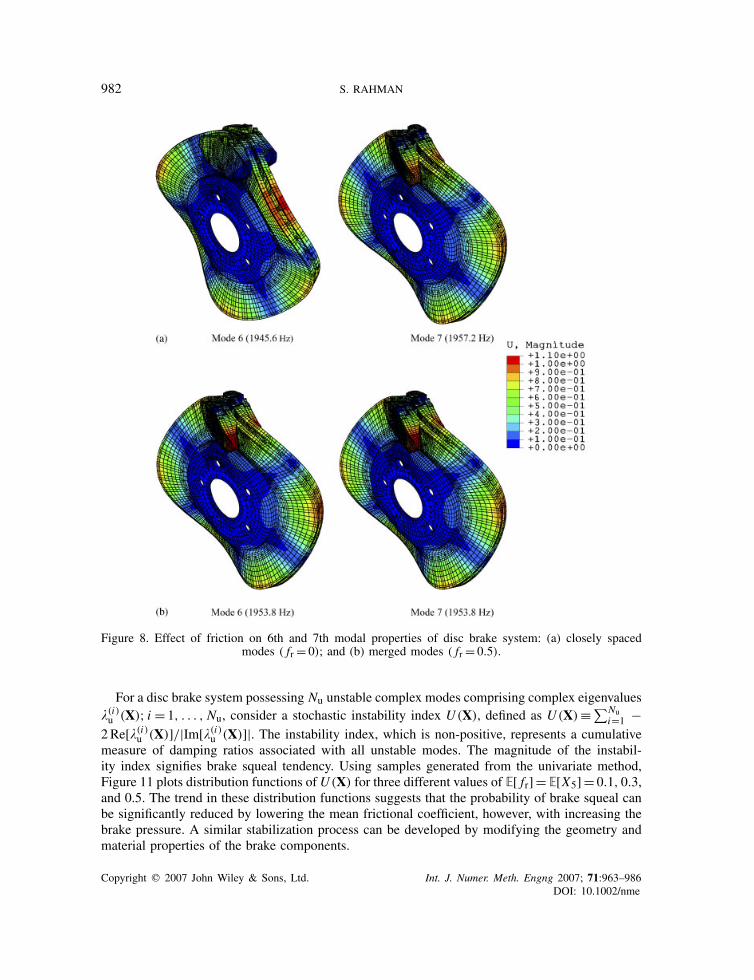
In calculating eigenvalues, both deterministic and stochastic analyses were performed. Forthe deterministic eigenvalue analysis, all previously defined random input except the frictionalcoefficient were fixed at their mean values. Two separate eigensolutions, one without friction( fr = 0) and the other with friction ( fr = 0.5), were obtained. When fr = 0, the stiffness matrix issymmetric and the system possesses only real modes. In the absence of friction, the 6th and 7thmode shapes, displayed in Figure 8(a), have frequencies of 1945.6 and 1957.2Hz, respectively.These two, closely spaced, neighbouring modes merge when the friction is raised to fr = 0.5,leading to the mode shapes (real part) in Figure 8(b) with a common frequency of 1953.8Hz.More importantly, a complex eigenvalue associated with the 7th mode, one of the two mergedmodes, has a positive real part, which makes the mode unstable. Similar instabilities occur athigher frequencies of 3040.5, 8026.0, and 8997.6Hz when fr = 0.5. All of these instabilities canbe identified by plotting the real part versus the imaginary part (frequency) of the eigenvalues,as presented in Figure 9 for the first 55 eigenvalues evaluated here. These unstable modes arefrequently attributed to the dynamic instability of a disc brake system, creating unwanted noise,commonly known as brake squeal.

For the random input X with its statistical properties listed in Table II and E[ fr] = E[X5] = 0.5,the univariate method was employed to evaluate probabilistic characteristics of eigensolutions.The calculation of eigenvalues for a given input is equivalent to performing a large-scale finiteelement analysis (ABAQUS). Therefore, computational efficiency is a major practical requirementin solving the disc brake random eigenvalue problem. Figures 10(a) and (b) present marginalprobability densities of the real and imaginary (frequency) parts, respectively, of the first unstablemode. These probability densities quantify the effect of random input on the variability of importantmodal properties of a disc brake system. Marginal densities of remaining unstable frequencies canbe developed similarly.


982 S. RAHMAN

Figure 8. Effect of friction on 6th and 7th modal properties of disc brake system: (a) closely spacedmodes ( fr = 0); and (b) merged modes ( fr = 0.5).

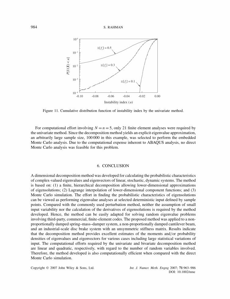
For a disc brake system possessing Nu unstable complex modes comprising complex eigenvalues�(i)u (X); i = 1, . . . , Nu, consider a stochastic instability index U (X), defined as U (X) ≡∑Nu

i=1 −2Re[�(i)

u (X)]/|Im[�(i)u (X)]|. The instability index, which is non-positive, represents a cumulative

measure of damping ratios associated with all unstable modes. The magnitude of the instabil-ity index signifies brake squeal tendency. Using samples generated from the univariate method,Figure 11 plots distribution functions ofU (X) for three different values of E[ fr] = E[X5] = 0.1, 0.3,and 0.5. The trend in these distribution functions suggests that the probability of brake squeal canbe significantly reduced by lowering the mean frictional coefficient, however, with increasing thebrake pressure. A similar stabilization process can be developed by modifying the geometry andmaterial properties of the brake components.



-200 -100 0 100 200Real part

0

2000

4000

6000

8000

10000

Imag

inar

y pa

rt (

freq

uenc

y), H

z

Figure 9. Complex eigenvalues of disc brake system for mean input ( fr = 0.5).

0 100 200 300 400 500

Re[λu

(1)]

0.000

0.002

0.004

0.006

0.008

0.010

Prob

abili

ty d

ensi

ty f

unct

ion Mean = 141.7

St. dev. = 48.83

[ fr] = 0.5

1000 1500 2000 2500 3000 3500 4000

Im[λu

(1)] (frequency), Hz

0.000

0.001

0.002

0.003

Prob

abili

ty d

ensi

ty f

unct

ion

[ fr] = 0.5

Mean = 1960.1 HzSt. dev. = 189.95 Hz

(a)

(b)

Figure 10. Probability density of complex eigenvalue of disc brake system at first unstable mode by theunivariate method: (a) real part; and (b) imaginary part (frequency).


984 S. RAHMAN

-0.10 -0.08 -0.06 -0.04 -0.02 0.00

Instability index (u)

10 -4

10 -3

10 -2

10 -1

10 0

P[U

(X)

< u

][ f

r] = 0.3

[ fr] = 0.5

[ fr] = 0.1

Figure 11. Cumulative distribution function of instability index by the univariate method.

For computational effort involving N = n = 5, only 21 finite element analyses were required bythe univariate method. Since the decomposition method yields an explicit eigenvalue approximation,an arbitrarily large sample size, 100 000 in this example, was selected to perform the embeddedMonte Carlo analysis. Due to the computational expense inherent to ABAQUS analysis, no directMonte Carlo analysis was feasible for this problem.

6. CONCLUSION

A dimensional decomposition method was developed for calculating the probabilistic characteristicsof complex-valued eigenvalues and eigenvectors of linear, stochastic, dynamic systems. The methodis based on: (1) a finite, hierarchical decomposition allowing lower-dimensional approximationsof eigensolutions; (2) Lagrange interpolation of lower-dimensional component functions; and (3)Monte Carlo simulation. The effort in finding the probabilistic characteristics of eigensolutionscan be viewed as performing eigenvalue analyses at selected deterministic input defined by samplepoints. Compared with the commonly used perturbation method, neither the assumption of smallinput variability nor the calculation of the derivatives of eigensolutions is required by the methoddeveloped. Hence, the method can be easily adapted for solving random eigenvalue problemsinvolving third-party, commercial, finite-element codes. The proposed method was applied to a non-proportionally damped spring–mass–damper system, a non-proportionally damped cantilever beam,and an industrial-scale disc brake system with an unsymmetric stiffness matrix. Results indicatethat the decomposition method provides excellent estimates of the moments and/or probabilitydensities of eigenvalues and eigenvectors for various cases including large statistical variations ofinput. The computational efforts required by the univariate and bivariate decomposition methodare linear and quadratic, respectively, with regard to the number of random variables involved.Therefore, the method developed is also computationally efficient when compared with the directMonte Carlo simulation.



APPENDIX A

For the discrete model of the beam, the 7× 7 mass, damping, and stiffness matrices are

M(X) = M(X)l

4

⎡⎢⎢⎢⎢⎢⎢⎢⎢⎢⎢⎢⎢⎢⎣

0 0 0 0 0 1 1

0 0 0 0 1 4 3

0 0 0 1 4 8 5

0 0 1 4 8 12 7

0 1 4 8 12 16 9

1 4 8 12 16 20 11

4 8 12 16 20 24 13

⎤⎥⎥⎥⎥⎥⎥⎥⎥⎥⎥⎥⎥⎥⎦

C(X) = C(X)

l

⎡⎢⎢⎢⎢⎢⎢⎢⎢⎢⎢⎢⎢⎢⎣

0 0 0 0 0 0 0

0 0 0 0 0 0 0

0 0 0 0 0 0 0

0 0 0 0 0 0 0

0 0 0 0 0 0 0

0 0 0 0 0 0 0

1 0 0 0 0 0 0

⎤⎥⎥⎥⎥⎥⎥⎥⎥⎥⎥⎥⎥⎥⎦

(A1)

and

K(X) = M(X)g

2

×

⎡⎢⎢⎢⎢⎢⎢⎢⎢⎢⎢⎢⎢⎢⎢⎣

0 0 0 0 k6 −2k6 + 1 k6 − 1

0 0 0 k5 −2k5 + 3 k5 − 2 −1

0 0 k4 −2k4 + 5 k4 − 2 −2 −1

0 k3 −2k3 + 7 k3 − 2 −2 −2 −1

k2 −2k2 + 9 k2 − 2 −2 −2 −2 −1

−2k1 + 11 k1 − 2 −2 −2 −2 −2 −1

K − 2 −2 −2 −2 −2 −2 −1

⎤⎥⎥⎥⎥⎥⎥⎥⎥⎥⎥⎥⎥⎥⎥⎦

(A2)

respectively, where ki (X) = 2ki (X)/(M(X)gl), K (X)= 2K (X)/(M(X)gl), and g is the accelera-tion due to the gravity.


986 S. RAHMAN

ACKNOWLEDGEMENTS

The author would like to acknowledge financial support from the U.S. National Science Foundation underGrant No. DMI-0355487. The author also thanks Dr A. Bajer of ABAQUS, Inc. for providing valuableinsights on disc brake analysis in Example 3.

REFERENCES

1. Boyce WE. Probabilistic Methods in Applied Mathematics I. Academic Press: New York, NY, 1968.2. Shinozuka M, Astill CJ. Random eigenvalue problems in structural analysis. AIAA Journal 1972; 10(4):456–462.3. Zhang J, Ellingwood B. Effects of uncertain material properties on structural stability. Journal of Structural

Engineering 1995; 121(4):705–714.4. Mehlhose S, Vom Scheidt J, Wunderlich R. Random eigenvalue problems for bending vibrations of beams.

Zeitschrift fur Angewandte Mathematik und Mechanik 1999; 79:693–702.5. Grigoriu M. A solution of the random eigenvalue problem by crossing theory. Journal of Sound and Vibration

1992; 158(1):69–80.6. Nair PB, Keane AJ. An approximate solution scheme for the algebraic random eigenvalue problem. Journal of

Sound and Vibration 2003; 260(1):45–65.7. Adhikari S, Friswell MI. Random matrix eigenvalue problems in structural dynamics. International Journal for

Numerical Methods in Engineering 2006, in press.8. Ghosh D, Ghanem RG, Red-Horse J. Analysis of eigenvalues and modal interaction of stochastic systems. AIAA

Journal 2005; 43(10):2196–2201.9. Rahman S. A solution of the random eigenvalue problem by a dimensional decomposition method. International

Journal for Numerical Methods in Engineering 2006; 67:1318–1340.10. Caughey TK, O’Kelly MEJ. Classical normal modes in damped linear dynamic systems. ASME Journal of

Applied Mechanics 1965; 32:583–588.11. Adhikari S. Complex modes in stochastic systems. Advances in Vibration Engineering 2004; 3(1):1–11.12. Xu H, Rahman S. A generalized dimension-reduction method for multi-dimensional integration in stochastic

mechanics. International Journal for Numerical Methods in Engineering 2004; 61:1992–2019.13. Xu H, Rahman S. Decomposition methods for structural reliability analysis. Probabilistic Engineering Mechanics

2005; 20:239–250.14. Hoeffding W. A class of statistics with asymptotically normal distributions. Annals of Mathematical Statistics

1948; 19:293–325.15. Efron B, Stein C. The Jackknife estimate of variance. Annals of Statistics 1981; 9:586–596.16. Sobol IM. Theorems and examples on high dimensional model representations. Reliability Engineering and

System Safety 2003; 79:187–193.17. Rabitz H, Alis O. General foundations of high dimensional model representations. Journal of Mathematical

Chemistry 1999; 25:197–233.18. Li G, Wang SW, Rabitz H. Practical approaches to construct RS-HDMR component functions. Journal of Physical

Chemistry A 2002; 106:8721–8733.19. Li G, Rosenthal C, Rabitz H. High dimensional model representations. Journal of Physical Chemistry A 2001;

105:7765–7777.20. Li G, Wang SW, Rosenthal C, Rabitz H. High dimensional model representations generated from low dimensional

data samples—I. mp-Cut-HDMR. Journal of Mathematical Chemistry 2001; 30:1–30.21. Puig B, Akian JL. Non-Gaussian simulation using hermite polynomial expansion and maximum entropy principle.

Probabilistic Engineering Mechanics 2004; 19:293–305.22. Newland DE. Mechanical Vibration Analysis and Computation. Wiley: New York, NY, 1989.23. IMSL Numerical Libraries. User’s Guide and Theoretical Manual. Visual Numerics Corporate Headquarters,

San Ramon, CA, 2005.24. ABAQUS. User’s Guide and Theoretical Manual, Version 6.5. Hibbitt, Karlsson, and Sorenson, Inc.: Pawtucket,

RI, 2005.25. Bajer A, Belsky V, Zeng LJ. Combining a nonlinear static analysis and complex eigenvalue extraction in brake

squeal simulation. Proceedings of 21st Annual Brake Colloquium and Exhibition, SAE Paper no. 2003-01-3349.Hollywood, FL, 2003.


stochasticdynamicsystemswithcomplex …user.engineering.uiowa.edu/~rahman/ijnme_comrep.pdfoperators...

Documents