Stochastic Stability in the Best–Shot Game

Leonardo Boncinelli∗ Paolo Pin†

March 4, 2010

Abstract

The best–shot game applied to networks is a discrete model of many processes ofcontribution in local public goods. It has generally a wide multiplicity of equilibriathat we refine through stochastic stability. In this paper we show that, dependingon how we define the perturbations, i.e. the possible mistakes that agents can make,we can obtain very different set of stochastically stable equilibria. In particular andnon–trivially, if we assume that the only possible source of error is that of an agentcontributing that stops doing so, then the only stochastically stable equilibria are themost inefficient ones.

JEL classification code: C72, C73, D85, H41.

Keywords: networks, best shot game, stochastic stability.

∗Dipartimento di Economia Politica, Universita degli Studi di Siena (Italy).†Dipartimento di Economia Politica, Universita degli Studi di Siena (Italy). I acknowledge support from

the project Prin 2007TKLTSR ”Computational markets design and agent–based models of trading behavior”.email: pin3@unisi.it

1

1 Introduction

Let us start with an example.

Example 1. Ann, Bob, Cindy, Dan and Eve live in a suburb of a big city and they all prefer

to take private cars to reach downtown every working day. They could share the car but

they are not all friends together: Ann and Eve do not know each other but they both know

Bob, Cindy and Dan, who also don’t know each other. The network of relations is shown in

Figure 1. In a one–shot equilibrium (the first working day) they will end up sharing cars.

Any of our characters would be happy to give a lift to a friend, but we assume here that

non–linked people do not know each other and would not offer each others a lift. No one

would take the car if a friend is doing so, but someone would be forced to take it if none

of her/his friends is doing so. There is an efficient equilibrium in which Ann and Eve take

the car (and the other three take somehow a lift), and a more polluting one in which Bob,

Cindy and Dan take their car (offering a lift to Ann and Eve, who will choose one of them).

Cindy

Bob

Dan

Ann Eve

Figure 1: Five potential drivers in a network of relations.

Imagine to be in the efficient equilibrium. Now suppose that, even if they all agreed how

to manage the trip, in the morning Ann finds out that her car’s engine is broken and she

cannot start it. She will call the other three, who are however not planning to take the car

and will not be able to offer her a lift. As Ann does not know Eve, and Eve will be the

only one left with a car, Ann will have to wait for her own car to be repaired before she can

reach her workplace. Only if both cars of Ann end Eve break down, then Bob, Cindy and

2

Dan will take their cars, and we will shift to the inefficient equilibrium. It is easy to see that

if we start instead from the inefficient equilibrium, then we need three cars to break down

before we can induce Ann and Eve to get their own. In this sense the bad equilibrium is

more stable, as it needs a less likely event in order to be changed with another equilibrium.

�

In this paper we analyze the best shot game:1 in a fixed exogenous network of binary

relations, each node (player) may or may not provide a local public good. The best response

for each player is to provide the good if and only if no one of her neighbors is doing so.

In the previous example we have described an equilibrium where each player can take one

of two actions: take or not take the car. Then we have included a possible source of error :

the car may break down and one should pass from action ‘take the car’ to action ‘not take

the car’. Clearly we can also imagine a second type of error, e.g. if a player forgets that

someone offered her/him a lift and takes her/his own car anyway. We think however that

there are situations in which the first type of error is the only plausible one, as well as there

can be cases in which the opposite is true, and finally cases where the two are equally likely.

What we want to investigate in the present paper is how the likelihood of different kind

of errors may influence the likelihood of different Nash Equilibria. Formally, we will analyze

stochastic stability (Young, 1998) of the Nash equilibria of the best shot game, under different

assumptions on the perturbed Markov chain that allows the agents to make errors.

What we find is that, if only errors of the type described in the example are possible,

that is players can only make a mistake by not providing the public good even if that is

their best response in equilibrium, then the only stochastically stable Nash equilibria are

those (inefficient ones) that maximize the number of contributors. If instead also (or only)

the other type of error (i.e. provide the good even if it is a dominant action to free ride) is

admitted, then every Nash equilibrium is stochastically stable.

The best shot game is very similar to the local public goods game of Bramoulle and

Kranton (2007): they motivate their model with a story of neighborhood farmers, with

reduced ability to check each others’ technology (this is the network constrain), who can

invest in experimenting a new fertilizer. They assume that the action set of the players is

continuous on the non–negative numbers (how much to invest in the new risky fertilizer),

they define stable equilibria as those that survive small perturbations, and they find that

stable equilibria are specialized ones, in which every agent either contributes an optimal

amount (which is the same for all contributors) or free rides, so that their stable equilibria

1This name for exactly the same game comes from Galeotti et al. (2008), but it stems back to thenon–network application of Hirshleifer (1983)

3

look like the equilibria of the discrete best shot game.

The main difference between our setup and the one of Bramoulle and Kranton (2007)

is that in the best shot games that we study actions are discrete, errors, even if rare, are

therefore more dramatic and the concept of stochastic stability naturally arises. We think

that this stark model offers a valid intuition of why typical problems of congestion are much

more frequently observed in some coordination problems with local externalities. Most of

these problems deal with discrete choice. Traffic is an intuitive and appealing example,2 while

others are given in the introduction of Dall’Asta et al. (2009a). In such complex situations

we analyze those equilibria which are more likely to be the outcome of convergence, under

the effect of local positive externalities and the possibility of errors.

In next section we formalize the best shot game. Section 3 describes the general best

response dynamics that we apply to the game. In Section 1 we introduce the possibility of

errors through perturbed dynamics. The main theoretical analysis on the effects of different

assumptions is there. In Section 5 we enrich our research with numerical simulations that

allow for quantitative analysis and to a comparison between different network structures.

2 Best-Shot Game

We consider a finite set of agents I of cardinality n. Players are linked together in a fixed

exogenous network which is undirected and irreflexive; this network defines the range of a

local externality described below. We represent such network through a n × n symmetric

matrix G, where Gij = 1 means that agents i and j are linked together (they are called

neighbors), while Gij = 0 means that they are not. We indicate with Ni the set of i’s

neighbors (the number of neighbors of a node is called its degree and is also its number of

links).

Each player can take one of two actions, xi = {0, 1} with xi denoting i’s action. This

action is interpreted as contribution, and an agent i such that xi = 1 is called contributor.

Similarly, action 0 is interpreted as defection, and an agent i such that xi = 0 is called

defector.3 We will consider only pure strategies. A state of the system is represented by a

2Economic modelling of traffic have shown that simple assumptions can easily lead to congestion, evenwhen agents are rational and utility maximizers (see Arnott and Small, 1994). Moreover, if we consider thediscretization of the choice space, the motivation for the Logit model of McFadden (1973) were actually thetransport choices of commuting workers.

3As will be clear below, we are dealing with a local public good game, so probably free rider would be amore suitable term than defector. Nevertheless, in the public goods game also “defector” is often used.

4

vector x which specifies each agent’s action, x = (x1, . . . , xi, . . . , xn). The set of all states is

denoted with X.

Payoffs are not explicitly specified. We limit ourselves to the class of payoffs that generate

the same type of best reply functions.4 In particular, if we denote with bi agent i’s best reply

function that maps a state of the system into a payoff value, then:

bi(x) =

{1 if xj = 0 for all j ∈ Ni ,

0 otherwise.(P1)

We introduce some further notation in order to simplify the following exposition. We

define the set of satisfied agents at state x as S(x) = {i ∈ I : xi = bi(x)}. Similarly, the set

of unsatisfied agents at state x is U(x) = I \ S(x). We also refer to the set of contributors

as C(x) = {i ∈ I : xi = 1}, and to the set of defectors as D(x) = {i ∈ I : xi = 0}. We also

define intersections of the above sets: the set of satisfied contributors is SC(x) = S(x)∩C(x),

the set of unsatisfied contributors is UC(x) = U(x) ∩ C(x), the set of satisfied defectors is

SD(x) = S(x)∩D(x), and the set of unsatisfied defectors is UD(x) = U(x)∩D(x). Finally,

given any pair of states (x,x′) we indicate with K(x,x′) = {i ∈ I : xi = x′i} the set of agents

that keep the same action in both states, and we indicate with M(x,x′) = I \K(x,x′) the

set of agents whose action is modified between the states.

The above game is called best-shot game. A state x is a Nash equilibrium of the best-shot

game if and only if S(x) = I and consequently U(x) = ∅. We will call all the possible Nash

equilibria, given a particular network, as N ⊆ X.

The set N is always non–empty but typically very large. It is an NP–hard problem

to enumerate all the elements of N , and to identify, among them, those that maximize

and minimize the set C(x) of contributors. For extensive discussions on this points see

Dall’Asta et al. (2009b) and Dall’Asta et al. (2009a). Here we provide two examples, the

second one illustrates how even very homogeneous networks may display a large variability

of contributors in different equilibria.

Example 2. Figure 2 shows two of the three possible Nash equilibria of the same 5–nodes

network, where the five characters of our introductory example have now a different network

of friendships. �

4Note that it would be very easy to define specific payoffs that generate the best reply defined by equation(P1): imagine that the cost for contributing is c and the value of a contribution, either from an agent herselfand/or from one of her neighbors (players are satiated by one unit of contribution in the neighborhood), isV > c > 0.

5

Ann

Bob

Cindy

Dan

Eve

(a)

Ann

Bob

Cindy

Dan

Eve

(b)

Figure 2: Two Nash equilibria for a 5–nodes network. The dark blue stands for contribution,

while the light blue stands for defection.

Example 3. Consider the particular regular random network, of 20 nodes and degree 4,

that is shown in Figure 3. The relatively small size of this network allows us to count all its

Nash equilibria. There exist 132 equilibria: 1 with 4 contributors (Figure 3, left), 17 with 5

contributors, 81 with 6 contributors, 32 with 7 contributors, 1 with 8 contributors (Figure

3, right). �

3 Unperturbed Dynamics

We imagine a dynamic process in which the network G is kept fixed, while the actions x of

the nodes change.

At each time, which is assumed discrete and denoted with t, a play of the best-shot

game occurs. The state of the system at time t + 1 is supposed to depend, possibly in a

probabilistic way, only on the state of the system at time t. We can therefore define a Markov

chain (X,T ), where X is the finite state space and T is the transition matrix, where Txx′

denotes the probability to pass from state x to state x′. We assume that T satisfies the

following property, which formalizes the idea that all and only the unsatisfied agents can

have the possibility to change action:

Txx′ > 0 if and only if (i ∈M(x,x′)⇒ i ∈ U(x)) (P2)

6

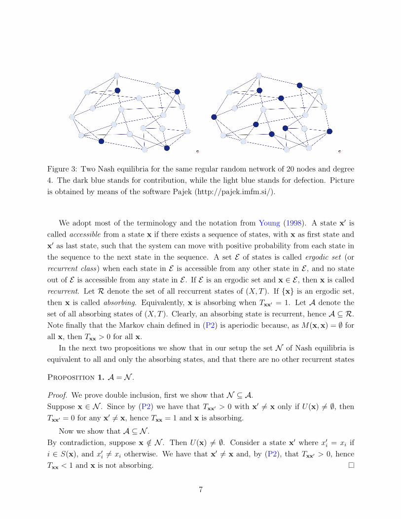
Figure 3: Two Nash equilibria for the same regular random network of 20 nodes and degree

4. The dark blue stands for contribution, while the light blue stands for defection. Picture

is obtained by means of the software Pajek (http://pajek.imfm.si/).

We adopt most of the terminology and the notation from Young (1998). A state x′ is

called accessible from a state x if there exists a sequence of states, with x as first state and

x′ as last state, such that the system can move with positive probability from each state in

the sequence to the next state in the sequence. A set E of states is called ergodic set (or

recurrent class) when each state in E is accessible from any other state in E , and no state

out of E is accessible from any state in E . If E is an ergodic set and x ∈ E , then x is called

recurrent. Let R denote the set of all reccurrent states of (X,T ). If {x} is an ergodic set,

then x is called absorbing. Equivalently, x is absorbing when Txx′ = 1. Let A denote the

set of all absorbing states of (X,T ). Clearly, an absorbing state is recurrent, hence A ⊆ R.

Note finally that the Markov chain defined in (P2) is aperiodic because, as M(x,x) = ∅ for

all x, then Txx > 0 for all x.

In the next two propositions we show that in our setup the set N of Nash equilibria is

equivalent to all and only the absorbing states, and that there are no other recurrent states

Proposition 1. A = N .

Proof. We prove double inclusion, first we show that N ⊆ A.

Suppose x ∈ N . Since by (P2) we have that Txx′ > 0 with x′ 6= x only if U(x) 6= ∅, then

Txx′ = 0 for any x′ 6= x, hence Txx = 1 and x is absorbing.

Now we show that A ⊆ N .

By contradiction, suppose x /∈ N . Then U(x) 6= ∅. Consider a state x′ where x′i = xi if

i ∈ S(x), and x′i 6= xi otherwise. We have that x′ 6= x and, by (P2), that Txx′ > 0, hence

Txx < 1 and x is not absorbing.

7

Proposition 2. A = R.

Proof. The first inclusion A ⊆ R follows from the definitions of A and R.

Now we show that R ⊆ A.

We prove that every element x which is not in A is also not in R. Suppose that x /∈ A. We

identify, by means of a recursive algorithm, a state x such that x is accessible from x, but x

is not accessible from x. This implies that x /∈ R.

By proposition 1 we know that A = N . Then x /∈ N and we have that U(x) 6= ∅. If

UC(x) 6= ∅, we define x′ ≡ x and we go to Step 1, otherwise we jump to Step 2.

Step 1. We take i ∈ UC(x′) and we define state x′′ such that x′′i ≡ 0 6= x′i = 1 and

x′′j ≡ x′j for all j 6= i.

Note that ||UC(x′′)|| < ||UC(x′)||. This is because of two reasons: first of all, i ∈ UC(x′) and

i /∈ UC(x′′); the second is that UC(x′′) ⊆ UC(x′), otherwise two neighbors contribute in x′′

and do not contribute in UC(x′), but that is not possible because C(x′′) ⊂ C(x′). Moreover,

by (P2) we have that Tx′x′′ > 0.

We redefine x′ ≡ x′′. Then, if UC(x′) = ∅ we pass to Step 2, otherwise we repeat Step 1.

Step 2. We know that UC(x′) = ∅. We take i ∈ UD(x) and we define state x′′ such that

x′′i ≡ 1 6= x′i = 0 and x′′j ≡ x′j for all j 6= i.

Note that ||UD(x′′)|| < ||UD(x′)||. This is because of two reasons: first of all, i ∈ UD(x′) and

i /∈ UD(x′′); the second is that UD(x′′) ⊆ UD(x′), otherwise two neighbors do not contribute

in x′′ and do contribute in UC(x′), but that is not possible because D(x′′) ⊂ D(x′).

We also note that still UC(x′′) = UC(x′) = ∅, since only i has become contributor and all i’s

neighbors are defectors.

By (P2) we have that Tx′x′′ > 0. Finally, if UD(x′′) 6= ∅ we redefine x′ ≡ x′′ and repeat Step

2, otherwise it means that x = x′′ and we have reached the goal of the algorithm.

The sequence of states we have constructed shows that x is accessible from x.

Since U(x′) = ∅, we have that Txx = 1 by (P2), and hence x is not accessible from x′.

An immediate corollary of Propositions 1 and 2 is that R = A = N .

We end this introductory section clarifying some points that could generate confusion as

there is ambiguity between the terminologies in game theoretical network economics (sur-

veyed in Jackson (2008)) and in the theory of stochastic stability (Young (1998)). The best

shot game is a one–shot game defined on a fixed network. In the topology of this network

we are interested only in characterizing neighborhoods. All the nodes of the network decide

simultaneously between contributing or not and every strategy profile in pure strategies will

de identified by a vector x ∈ X.

8

Then we define a dynamical system in discrete time, based on the best shot game, as is

done in the theory of stochastic stability. We call any element x as a state of the dynamical

system, and the rule in (P2) defines a Markov chain between those states. This Markov chain

can be represented as a directed network between the states, but should not be confused

with the original undirected network on which the game is played.5 We will use all the words

with a dynamic implication (e.g. accessible, path. . . ) only for the Markov chain.

The algorithm of the proof of Proposition 2 uses those transitions in T where only one

unsatisfied player changes its action. However, it should be noted that (P2) allows with

positive probability any change in which any subset of the unsatisfied nodes change.

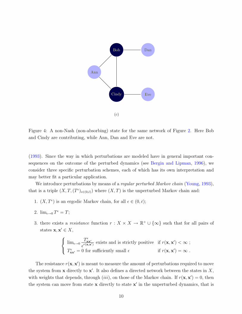
Example 4. Consider the network from Figure 2: both states (a) and (b) shown there are

absorbing, as they are Nash equilibria. Consider now the new state (c) on the same network,

shown in Figure 4: the satisfied nodes here are only the defectors Ann, Dan and Eve. Both

states (a) and (b) are accessible from state (c), but through different paths. To reach (a) from

(c), the unsatisfied contributor Cindy should turn to defection, so that Eve would become

(the only) unsatisfied and would be forced to become a contributor. To reach (b) from (c),

both the unsatisfied contributors Bob and Cindy should simultaneously turn to defection,6

then all five nodes would be unsatisfied. If we now turn to contribution exactly Ann, Dan

and Eve, we reach state (b). �

The diagram in Figure 5 sketches how the T dynamics works. The four nodes in the

figure represent the same agent, with the letters within each node indicating whether such

agent is a contributor (C) or a defector (D), and if she is satisfied (S) or unsatisfied (U).

Arrows represent all and only the possible changes in terms of cooperation/defection and

satisfaction/unstatisfaction that can occur to an agent when the T dynamics is applied.

4 Perturbed Dynamics

Given the multiplicity of Nash equilibria, we are uncertain about the final outcome of (X,T ),

that depends in part on the initial state and in part on the realizations of the probabilistic

passage from states to states. In order to obtain a more sharp prediction, which is inde-

pendent of the initial state, we introduce a small amount of perturbations and we use the

techniques developed in economics by Foster and Young (1990), Young (1993), Kandori et al.

5Such a network of all possible configurations, in which directed links are driven by best reply functions,is in the same spirit of meta–networks in Jackson and Watts (2002).

6This is not in contradiction with the algorithm defined in the proof of Proposition 2, because there thestarting state x is supposed to be a Nash equilibrium, while (c) is not.

9

Ann

Bob

Cindy

Dan

Eve

(c)

Figure 4: A non-Nash (non-absorbing) state for the same network of Figure 2. Here Bob

and Cindy are contributing, while Ann, Dan and Eve are not.

(1993). Since the way in which perturbations are modeled have in general important con-

sequences on the outcome of the perturbed dynamics (see Bergin and Lipman, 1996), we

consider three specific perturbation schemes, each of which has its own interpretation and

may better fit a particular application.

We introduce perturbations by means of a regular perturbed Markov chain (Young, 1993),

that is a triple (X,T, (T ε)ε∈(0,ε)) where (X,T ) is the unperturbed Markov chain and:

1. (X,T ε) is an ergodic Markov chain, for all ε ∈ (0, ε);

2. limε→0 Tε = T ;

3. there exists a resistance function r : X × X → R+ ∪ {∞} such that for all pairs of

states x,x′ ∈ X, limε→0T εxx′

εr(x,x′) exists and is strictly positive if r(x,x′) <∞ ;

T εxx′ = 0 for sufficiently small ε if r(x,x′) =∞ .

The resistance r(x,x′) is meant to measure the amount of perturbations required to move

the system from x directly to x′. It also defines a directed network between the states in X,

with weights that depends, through (iii), on those of the Markov chain. If r(x,x′) = 0, then

the system can move from state x directly to state x′ in the unperturbed dynamics, that is

10

. .^

. .^

. ._

. ._

Figure 5: Single node dynamics in T . Dark blue stands for contribution, light blue stands

for defection, . .^ stands for being satisfied, . ._ stands for being unsatisfied.

Txx′ > 0. If r(x,x′) = ∞, then the system cannot move from x directly to x′ even in the

presence of perturbations, that is T εxx′ = 0 for ε sufficiently small.

Even if T and r are defined on all the possible states of X, we can limit our analysis

to the absorbing states only, which are all and only the recurrent ones (Proposition 2).

This technical procedure is illustrated in Young (1998) and simplifies the complexity of the

notation, without loss of generality. Given x,x′ ∈ A, we define r∗(x,x′) as the minimum

sum of the resistances between absorbing states over any path starting in x and ending in

x′.

Given x ∈ A, an x-tree on A is a subset of A×A that constitutes a tree rooted at x.7 We

denote such x-tree with Fx and the set of all x-trees with Fx. The resistance of an x-tree,

denoted with r∗(Fx), is defined to be the sum of the resistances of its edges, that is:

r∗(Fx) ≡∑

xx′∈Fx

r∗(x,x′) .

Finally, the stochastic potential of x is defined to be

ρ(x) ≡ min{r∗(Fx) : Fx ∈ Fx} .7By tree we will refer only to this structure between absorbing states, and in no way to the topology of

the underlying exogenous undirected network on which the best shot game is played.

11

A state x is said stochastically stable (Foster and Young, 1990) if ρ(x) = min{ρ(x) : x ∈ A}.Intuitively, stochastically stable states are those and only those states that the system can

occupy after very long time has elapsed in the presence of very small perturbations.8

For the sake of an easy interpretation, we follow Samuelson (1997) and we derive the

perturbed transition matrix T ε by post-multiplying the unperturbed transition matrix T

with a perturbations matrix P ε, where P εxx′ is the probability that perturbations move the

system from x to x′. Therefore,

T εxx′ =∑x′′∈X

Txx′′P εx′′x′ . (1)

We consider three types of perturbations in Subsections 4.1, 4.2 and 4.3.

4.1 Perturbations affect only the agents that are playing action 0

We assume that every agent playing action 0 can be hit by a perturbation which makes her

switch action to 1. Each perturbation occurs with an i.i.d. probability ε. No agent playing

action 1 can be hit by a perturbation. We indicate the perturbations matrix with P 0,ε and

the resulting perturbed transition matrix with T 0,ε. It turns out that

P 0,εxx′ =

{ε||M(x,x′)||(1− ε)||D(x,x′)−M(x,x′)|| if C(x) ⊆ C(x′)

0 otherwise(2)

We check that (X,T, (T 0,ε)ε∈(0,ε)) is indeed a regular perturbed Markov chain.

1. (X,T 0,ε) is ergodic for all positive ε; this can be seen applying the last sufficient condi-

tion for ergodicity in Fudenberg and Levine (1998, appendix in chap. 5), once we take

into account that i) A = R by Proposition 2, and ii) r∗(x,x′) <∞ for all x,x′ ∈ A by

the following Lemma 1.

2. limε→0 T0,ε = T , since limε→0 P

0,ε is equal to the identity matrix.

3. The resistance function is

r0(x,x′) =

{||SD(x) ∩M(x,x′|| if SC(x) ∩M(x,x′) = ∅∞ otherwise

(3)

In fact,

8For a formal statement see Young (1993).

12

(a) if r(x,x′) = ∞, then SC(x) ∩M(x,x′) 6= ∅ and there is no way to go from x

to x′, since no satisfied agent can change in the unperturbed dynamics and no

contributor can be hit by a perturbation, hence T εxx′ = 0 for every ε;

(b) if r(x,x′) < ∞, then T 0,εxx′ has the same order of εr(x,x

′) when ε approaches zero;

in fact, the agents in U(x)∩M(x,x′) can change when T is applied, the agents in

SD(x) ∩M(x,x′) can change when P ε is applied (and only then), and no agent

is left since SC(x) ∩M(x,x′) = ∅.

The diagram in Figure 6 shows how the T ε dynamics works when (3) holds. Again, blue

dashed lines stand for changes that are possible only by perturbation. With respect to the

diagram in Figure ?? we have two blue dashed lines missing, those going from a satisfied

contributor to a satisfied defector and to an unsatisfied defector.

. .^

. .^

. ._

. ._

Figure 6: Single node dynamics in T ε under (2). Dark blue stands for contribution, light

blue stands for defection, . .^ stands for being satisfied, . ._ stands for being unsatisfied, blue

dashed lines stands for changes that are possible only by perturbation.

In the next remark we provide a lower bound for the resistance to move between Nash

equilibria under this perturbation scheme, and we then use such remark in Proposition 3.

Remark 1. When (2) holds, r∗(x,x′) ≥ 1 for all x,x′ ∈ N .

The following lemma, which is of help in the proof of Proposition 3, shows that under this

perturbation scheme any two absorbing states are connected through a sequence of absorbing

states, with each step in sequence having resistance 1.

13

Lemma 1. When (2) holds, for all x,x′ ∈ A, x 6= x′, there exists a sequence x0, . . . ,xs, . . . ,xk,

with xs ∈ A for 0 ≤ s ≤ k, x0 = x and xk = x′, such that r∗(xs,xs+1) = 1 for 0 ≤ s < k.

Proof. We denote with k the cardinality of the set of contributors in x′ that are defectors in

x, namely k = ||C(x′) ∩D(x)||. Since vecx 6= x′, we have that k ≥ 1. We set x0 = x.

For 0 ≤ s < k:

Take i ∈ C(x′) ∩ D(xs). We define state x such that xi ≡ 1 6= xsi = 0 and xj ≡ xij for all

j 6= i. Note that r(xi, x) = 1. We now define state xi+1 such that xi+1j ≡ 0 for all j ∈ Ni, and

xi+1j ≡ xj for all j /∈ Ni. Note that r(x,xi+1) = 0. By Lemma 2 in Dall’Asta et al. (2009a)

we have that xi+1 ∈ N , and hence xi+1 ∈ A by Lemma 1. Therefore, r∗(xi,xi+1) = 1.

Note that, since i /∈ D(xi+1) and (j ∈ Ni ⇒ j ∈ D(x′)), then ||C(x′) ∩ D(xi+1)|| =

||C(x′) ∩D(xi)|| − 1. Therefore, ||C(x′) ∩D(xk)|| = 0, and this means that xk = x′.

Next proposition provides a characterization of stochastically stable states under (3).

Proposition 3. When (2) holds, a state x is stochastically stable in (X,T, (T ε)ε∈[0,ε)) if and

only if x ∈ N .

Proof. We first show that x ∈ N implies x stochastically stable. Theorem 2 in Samuelson

(1994) implies that if x′ is stochastically stable, x ∈ A, r∗(x′,x) is equal to the minimum

resistance between recurrent states, then x is stochastically stable. Since at least one re-

current state must be stochastically stable, Proposition 2 implies that there must exist an

absorbing state x′ that is stochastically stable. For any x ∈ N , if x = x′ we are doone. If

x 6= x′, then we by Proposition 1 we can use Lemma 1 to say that there exists a sequence of

absorbing states from x′ to x. Remark 1, together with Propositions 2 and 1, implies that

1 is the minimum resistance between recurrent states. A repeated application of Theorem

2 in Samuelson (1994) shows that each state in the sequence is stochastically stable, and in

particular the final state x.

It is trivial to show that x stochastically stable implies x ∈ N . By contradiction, suppose

x /∈ N . Then, by Propositions 2 and 1, x /∈ R, and hence cannot be stochastically stable.

4.2 Perturbations affect only the agents that are playing action 1

We assume that avery agent playing action 1 can be hit by an i.i.d. perturbation ε, while no

agent playing action 0 is susceptible to perturbations. We denote the perturbations matrix

with P 1,ε and the resulting perturbed transition matrix with T 1,ε. It turns out that

P 1,εxx′ =

{ε||M(x,x′)||(1− ε)||C(x,x′)−M(x,x′)|| if D(x) ⊆ D(x′)

0 otherwise(4)

14

We check that (X,T, (T 1,ε)ε∈(0,ε)) is indeed a regular perturbed Markov chain.

1. (X,T 1,ε) is ergodic for all positive ε by the same argument of the corresponding point

in the previous Subsection 4.1, once we replace Lemma 2 to Lemma 1.

2. limε→0 T1,ε = T , since limε→0 P

1,ε is equal to the identity matrix.

3. The resistance function is

r1(x,x′) =

{||SC(x) ∩M(x,x′)|| if SD(x) ∩M(x,x′) = ∅∞ otherwise

(5)

In fact, analogously to what happens for Subsection 4.1,

(a) if r(x,x′) =∞, then SD(x)∩M(x,x′) 6= ∅ and there is no way to go from x to x′,

since no satisfied agent can change in the unperturbed dynamics and no defector

can be hit by a perturbation, hence T εxx′ = 0 for every ε;

(b) if r(x,x′) < ∞, then T 0,εxx′ has the same order of εr(x,x

′) when ε approaches zero;

in fact, the agents in U(x) ∩M(x,x′) can change when T is applied, the agents

in SC(x)∩M(x,x′) can change when P ε is applied (and only then), and no agent

is left since SD(x) ∩M(x,x′) = ∅.

The diagram in Figure 7 shows how the T ε dynamics works when (5) holds. With respect

to the diagram in figure ?? we have three blue dashed lines missing, the two going from a

satisfied defector to a satisfied contributor and to an unsatisfied contributor, and the one

(the most surprising) going from a satisfied contributor to a satisfied defector.

This remark plays the same role of Remarks 3 and 1.

Remark 2. When (4) holds, r∗(x,x′) ≥ 1 for all x,x′ ∈ N .

The following Lemma shows that the resistance between any two absorbing states is

equal to the number of contributors that must change to defection. This result is less trivial

than it might appear: it shows that there is no possibility that by changing only some of

the contributors to defectors, the remaining ones are induced to change by the unperturbed

dynamics.

Lemma 2. When (4) holds, for all x,x′ ∈ A, r∗(x,x′) = ||C(x) ∩D(x′)||.

Proof. We first show that r∗(x,x′) ≥ ||C(x)∩D(x′)||. By contradiction, suppose r∗(x,x′) <

||C(x) ∩D(x′)||. Then, some i ∈ C(x) ∩D(x′) must switch from contribution to defection

15

. .^

. .^

. ._

. ._

Figure 7: Single node dynamics in T ε under (4). Dark blue stands for contribution, light

blue stands for defection, . .^ stands for being satisfied, . ._ stands for being unsatisfied, blue

dashed lines stands for changes that are possible only by perturbation.

along a path from x to x′ by best reply to the previous state. This requires that in the

previous state there must exist some j ∈ Ni that contributes. However, j ∈ D(x) and j

can never change to contribution as long as i is a contributor, neither by best reply nor by

perturbation when (5) holds.

We now show that r∗(x,x′) ≤ ||C(x)∩D(x′)||. Define state x such that xi ≡ 0 6= xi = 1

for all i ∈ C(x) ∩D(x′), and xi ≡ xi otherwise. Note that r(x, x) = ||C(x) ∩D(x′)||. Note

also that bi(x) = 1 for all i ∈ C(x′) ∩ D(x). This means that r(x,x′) = 0, and therefore

r∗(x,x′) ≤ r(x, x) + r(x,x′) = ||C(x) ∩D(x′)||.

We now use the above Lemma 2 to relate algebraically the resistance move away from x

to x′ to the resistance to come back x′ to x.

Lemma 3. When (4) holds, for all x,x′ ∈ A, r∗(x,x′) = r∗(x′,x) + ||C(x)|| − ||C(x′)||.

Proof. From Lemma 2 we know that r∗(x,x′) = ||C(x)∩D(x′)||. Note that ||C(x)∩D(x′)|| =||C(x)|| − ||C(x) ∩ C(x′)||. Always from Lemma 2 we also know that r∗(x,x′) = ||C(x′) ∩D(x)|| = ||C(x′)|| − ||C(x) ∩C(x′)||, from which ||C(x) ∩C(x′)|| = C(x′)− r∗(x′,x), which

substituted in the former equality gives the desired result.

16

Lemma 3 allows us to provide in next Proposition a characterization of stochastically

stable states under (5).

Proposition 4. When (4) holds, a state x is stochastically stable in (X,T, (T ε)ε∈[0,ε)) if and

only if x ∈ arg maxx′∈N ||C(x′)||.

Proof. We first prove that only a state in arg maxx′∈N ||C(x′)|| may be stochastically stable.

Ad absurdum, suppose ||C(x)|| /∈ arg maxx′∈N ||C(x′)|| and x is stochastically stable. There

must exist x′ such that ||C(x′)|| > ||C(x)||. Take an x-tree Fx. Consider the path in Fx

going from x′ to x, that is the unique {(x0,x1), . . . , (xk−1,xk)} such that x0 = x′, xk = x,

and (xi,xi+1) ∈ Fx for all i ∈ {0, k − 1}. We now modify Fx by reverting the path from x′

to x, so we define Fx′ = (Fx \ {(xi,xi+1) : i ∈ {0, k − 1}}) ∪ {(xi+1,xi) : i ∈ {0, k − 1}},which is indeed an x′-tree. It is straightforward that r∗(Fx′) = r∗(Fx)−

∑k−1i=0 r

∗(xi,xi+1) +∑k−1i=0 r

∗(xi+1,xi). Applying Lemma 3 we obtain r∗(Fx′) = r∗(Fx) +∑k−1

i=0 (||C(xi+1)|| −||C(xi)||), that simplifies to r∗(Fx′) = r∗(Fx)+||C(x)||−||C(x′)||). Since ||C(x′)|| > ||C(x)||,then r∗Fx′ < r∗Fx. In terms of stochastic potentials, this implies that ρ(x′) < ρ(x), against

the hypothesis that x is stochastically stable.

We now prove that any state in arg maxx′∈N ||C(x′)|| is stochastically stable. Since

at least one stochastically stable state must exist, from the above argument we conclude

that there exists x ∈ arg maxx′∈N ||C(x′)|| that is stochastically stable. Take any other

x′ ∈ arg maxx′∈N ||C(x′)||. Following exactly the same reasoning as above we obtain that

ρ(x′) = ρ(x). Since ρ(x) is minimum, ρ(x′) is minimum too, and x′ is hence stochastically

stable.

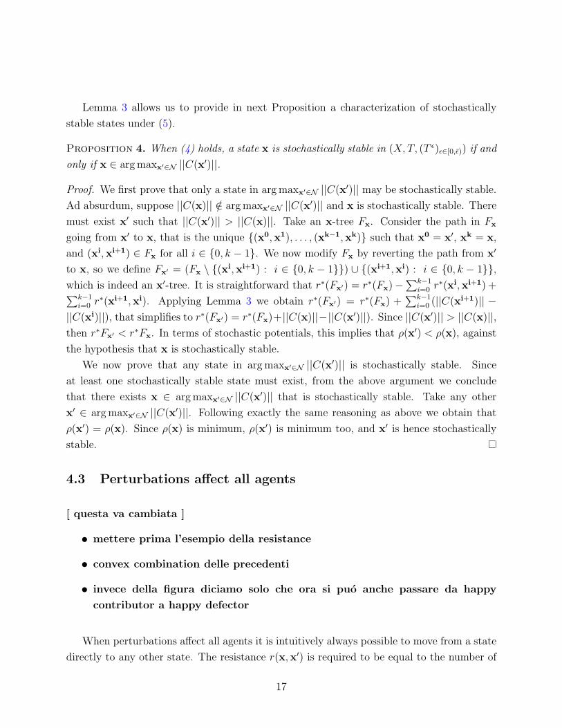
4.3 Perturbations affect all agents

[ questa va cambiata ]

• mettere prima l’esempio della resistance

• convex combination delle precedenti

• invece della figura diciamo solo che ora si puo anche passare da happy

contributor a happy defector

When perturbations affect all agents it is intuitively always possible to move from a state

directly to any other state. The resistance r(x,x′) is required to be equal to the number of

17

agents playing an action in x′ that is (i) different from the action in x and (ii) not obtainable

as best reply response to x. We can easily summarize this in an algebraic formula: for all

x ∈ X,

r(x,x′) ≡ ||S(x) ∩M(x,x′)|| =∑i∈I

(x′i − xi)(x′i − bi(x)) (P3)

In other words, r(x,x′) is the number of agents that are required to change action making

a mistake in order to pass from x to x′. Note that there exists a unique resistance function

that satisifes (P3), which can then be considered as a definition.

Example 5. Consider the following family of perturbed transition matrices: for all ε ∈ (0, ε),

T ε =∑x′′∈X

Txx′′T εx′′x′ ,

with

T εx′′x′ ≡ εd10(x′′,x′)(1− ε)n−d10(x′′,x′),

d10(x′′,x′) ≡ ||M(x′′,x′)|| =∑i∈I

(x′i − x′′i )(x′i − x′′i ).

Here the unperturbed transition matrix is first applied, and then each agent independently

switches action with probability ε. It is easy to check that such (X,T, (T ε)ε∈(0,ε)) is indeed a

regular perturbed Markov chain.

1. (X,T ε) is ergodic for all positive ε; this can be seen applying the last sufficient condition

for ergodicity in (Fudenberg and Levine, 1998, appendix in chap. 5), once we take into

account that i) A = R by Proposition 2, and ii) r∗(xx′) < ∞ for all x,x′ ∈ A by the

following Lemma 1.

2. limε→0 Tε = T , since limε→0 T

ε is equal to the identity matrix.

3. Function r satisfying (P3) is a resistance function, since the agents in U(x)∩M(x,x′)

can change when T is applied, while the agents in S(x) ∩M(x,x′) can change only

when T ε is applied.

The last point above shows also that the resistance function of the regular perturbed Markov

chain under consideration satisfies indeed (P3). �

The following simple remark states a lower bound for the resistance to move between Nash

equilibria, and it is of help to establish which states have minimum stochastic potential.

Remark 3. When (P3) holds, r∗(x,x′) ≥ 1 for all x,x′ ∈ N .

18

Next proposition provides a characterization of stochastically stable states under (P3).

Proposition 5. When (P3) holds, a state x is stochastically stable in (X,T, (T ε)ε∈[0,ε)) if

and only if x ∈ N .

Proof. It follows from Proposition 3 when we replace Remark 3 to Remark 1.

5 Simulation Results

In the previous section we have shown that under (5)-type of perturbations, at the limit of

vanishing perturbations, the regular perturbed Markov chain tends to Nash equilibria with

maximum number of contributors, while under (3)-type and (P3)-type of perturbations,

at the same limit, every Nash equibrium is visited with positive probability in the long

run. These results refer to the time-asymptotyc behavior when the amount of perturbations

appproaches zero. We are here concerned to understand what happens in terms of average

contribution in the presence of small but finite amount of perturbations, after very long

time has elapsed for time–asymptotic behavior to be relevant. This kind of investigation is

difficult to be done by mathematical deduction for general classes of networks, and therefore

we rely on computer–based simulations.

5.1 A completely controlled environment

We start, as a benchmark case, from a completely controlled environment: the regular

random network shown in Example 3. For this network we know exactly that the maximum

Nash equilibrium has a percentage of 40% of contributors (8 out of 20), but the percentage

of contributors in Nash equilibria ranges down to 20%. Figure 8 shows the average number

of contributors for the regular perturbed Markov chains from Examples ?? (the (3)-type

of perturbations) and ?? (the (5)-type of perturbations). We have considered the average

percentage of contributors over a large span of 106 time steps, for different values of the ε

i.i.d. probability of a single node making an error, as illustrated in Examples ?? and ??. This

has been iterated for 10 different time spans for each value of ε on a discrete grid of small

values, for the two regular perturbed Markov chains.By so doing we perform a comparative

static between steady states, which is analogous as approaching first the limit on the time

dimension, and then the limit on the probability ε of an error (see ? for the importance of

the order in which limits are taken).

It is clear from a comparison of the two panels in Figure 8 that the average contribution

in the (3)-type of perturbations lies always below the (5)-type. This is important since it

19

Figure 8: Box–plots over 10 runs of stochastic processes over the same regular random

network of Figure 3. In both panels x–axis is the i.i.d. probability of an error and y–axis is

the percentage of contributors averaged over 106 time steps. Left panel: (5)–type stochastic

process. Right panel: (3)–type stochastic process.

allows to extend the conclusion that we obtain comparing, at one side, either Proposition 3

or Proposition 5, and at the other Proposition 4, to non-vanishing amounts of perturbations:

(5)-type of perturbations favors contribution. Moreover, we note that the slope of the relation

between average contribution and the amount of perturbations is higher for (5)-type of

perturbations. This is likely to be related to the fact that in such a case there is the

tendency for the system to move to equilibria with maximum number of contributors as the

amount of perturbations approaches zero, while such tendency is absent for the other two

types of perturbations (Propositions 5, 3 and 4).

In the case of the (5)-type, moreover, the limit seems to converge linearly to the threshold

value that we know to be the maximum possible in a Nash equilibrium, as is shown for the

limit by Proposition 4. The higher variance is due to the fact that, as ε converges to 0,

perturbations on the network are much more rare on the same time–span, and the regular

perturbed Markov chain changes sites less frequently.

Commento sulla varianza maggiore di 1→ 0.

Finally, a remark concerns the downward slope of the relation between the amount ε

of perturbations and the average contribution, also for the (3)-type of perturbations in the

left panel. Since only agents that are playing action 0 can make a mistake, one would first

think that the relation should be upward sloping. However, as a consequence of an agent’s

switch from 0 to 1 we have that other agents can switch their action, possibly leading to

an equilibrium with an overall lower number of contributors. That the latter occurrence is

indeed what is more likely to happen is a matter of fact for which we do not have a convincing

20

argument.

5.2 Random networks

The nice monotonicity of previous simulations could be the consequence of a very particular

single network. We compare then two well–known classes of random networks: regular

random networks and scale–free networks.9 For the two types of networks, and for the

(3)-type and (5)-type of stochastic processes, we run 20 simulations, one for each different

realization of the two classes of random networks.10 The size of networks is always 50 nodes,

that is a trade-off between computational tractability and variability.

Figure 9 reports the results for the regular perturbed Markov chain from Example ?? (the

(3)-type of perturbations). Figure 10 reports instead the results for the regular perturbed

Markov chain from Example ?? (the (5)-type of perturbations). In the graphs on the top

of the figures we used networks that are realizations of a regular random network (with a

time span of 106 time–steps), and in the graphs on the bottom of the figures we repeated

the simulations using realizations of a scale-free network (for which a smaller time span of

105 time–steps was sufficient to get a reasonable stationarity). Here we reported also, in the

left panels, another average quantity on the time–spans, which is the percentage unsatisfied

agents across the regular perturbed Markov chains, that visits also non–equilibrium states.

Let us describe and compare Figures 9 and 10. We note that the downward and linear

slope of the relation between the amount of perturbations and the average contribution is

still present, as discussed for Figure 8. We do not know if the left panels of Figure 10 are

actually approaching the exact maximum number of contributors in a Nash equilibrium, as

we can claim for sure for the left panel of Figure 8. However, the left–top panel of Figure 10

approaches well the analytical predictions of Dall’Asta et al. (2009b).

In both figures the average contribution and its variability are always higher for scale-free

networks. This is essentially due to the more asymmetric structure that scale-free networks

have, if compared to regular random networks. In the former there are equilibria where

9Newman (2003) and Jackson and Rogers (2007) show that regular random networks and scale–freenetworks miss some important statistical properties of real–world networks, such as clustering, as the numberof nodes becomes large. For relatively small networks as the ones we are considering, this is not true andthe two types of networks may be thought of as representatives of homogeneous and heterogeneous degreedistributions.

10For regular random networks we adopted the procedure from McKay and Wormald (1990), while forscale-free networks we followed the preferential attachment model by Barabasi and Albert (1999). We didnot use the same realization for the underlying network in order not to have results depending on a fortuitousrealization.

21

Figure 9: Average quantities over large time spans of the (3)–type stochastic process. In

all four panels x–axis is the i.i.d. probability of an error. Top–left panel: y–axis is the

percentage of contributors averaged over 106 time steps (box plots over 20 different regular

random networks of 50 nodes and degree 4). Top–right panel: y–axis is the percentage of

unsatisfied nodes averaged over 106 time steps (box plots over the same sample). Lower

panels differ from the above as the quantities are averaged over only 105 time steps, and box

plots are over 20 different scale–free networks of 50 nodes and average degree 4.

few highly connected agents contribute, and others where many scarcely connected agents

contribute. In the latter, instead, all equilibria are less diverse since they involve agents that

all have the same number of connections.

We make some further remarks concerning the relation between the proportion of unsat-

isfied agents and the amount of perturbations. Its upward slope is rather trivial: starting

from equilibria, where by definition no agent is unsatisfied, an increase in the amount of per-

turbations clearly raises the proportion of unsatisfied agents (those who made the mistake

and possibly some of their neighbors). What is more interesting is the different slope for the

two types of perturbations. Part of the explanation is related to the different proportions of

agents that are susceptible of making mistakes. This leads, for instance, to conclude (as we

checked) that with (P3)-type of perturbations the slope is the highest. Another reason that

probably works in favor of a lower slope for (5)-type of perturbations with respect to (3)-type

of perturbations is that a mistake of the former type leads to changes that are limited to

22

Figure 10: Average quantities over large time spans of the (5)–type stochastic process. All

four panels have respectively the same legend as in Figure 9.

the neighborhood of order 1 of the original node, while a mistake of the latter type leads to

changes that are limited to the neighborhood of order 2 of the original node (see Lemma 2

in Dall’Asta et al., 2009a). Therefore we may roughly say that (3)-type of perturbations has

a larger impact than (5)-type of perturbations, and that is probably responsible for part of

the difference in slope.

5.3 Perturbation affects all agents

[To be completed]

6 Discussion

Results in Subsection 4.1 are given when (2) holds. Actually, they are valid for any regular

perturbed Markov chain whose resistance function is (3).

Results in Subsection 4.2 are given when (4) holds. Actually, they are valid for any

regular perturbed Markov chain whose resistance function is (5). [To be completed]

23

6.1 Relation with Bergin and Lipman (1996)

[To be completed]

Esempio che hai detto mentre si prendeva il caffe

6.2 Relation with Ellison (2000)

[To be completed]

Minimal spanning tree? coradius?

6.3 Relation with Bramoulle and Kranton (2007)

[To be completed]

6.4 Future research

[To be completed]

References

Arnott, R. and K. Small (1994). “The Economics of Traffic Congestion”. American Scien-

tist 82 (5), 446–455.

Barabasi, A.-L. and R. Albert (1999). “Emergence of Scaling in Random Networks”. Sci-

ence 286, 509–512.

Bergin, J. and B. L. Lipman (1996). “Evolution with State-Dependent Mutations”. Econo-

metrica 64, 943–956.

Bramoulle, Y. and R. Kranton (2007). “Public Goods in Networks”. Journal of Economic

Theory 135, 478–494.

Dall’Asta, L., P. Pin, and A. Ramezanpour (2009a). “Optimal equilibria of the best shot

game”. Working Papers of the FEEM Foundation (n.33.2009).

24

Dall’Asta, L., P. Pin, and A. Ramezanpour (2009b). “Statistical Mechanics of maximal

independent sets”. Physical Review E – accepted for publication.

Foster, D. and H. P. Young (1990). “Stochastic Evolutionary Game Dynamics”. Theoretical

Population Biology 38, 219–232.

Fudenberg, D. and D. K. Levine (1998). The Theory of Learning in Games. Cambridge,

Massachussets: the MIT Press.

Galeotti, A., S. Goyal, M. Jackson, F. Vega-Redondo, and L. Yariv (2008). “Network

Games”. The Review of Economic Studies , forthcoming.

Hirshleifer, J. (1983). “From Weakest-Link to Best-Shot: The Voluntary Provision of Public

Goods”. Public Choice 41 (3), 371–386.

Jackson, M. (2008). Social and Economic Networks. Princeton: Princeton University Press.

Jackson, M. and A. Watts (2002). “The Evolution of Social and Economic Networks”.

Journal of Economic Theory 106 (2), 265–296.

Jackson, M. O. and B. W. Rogers (2007). “Meeting Strangers and Friends of Friends: How

Random Are Social Networks?”. American Economic Review 97, 890–915.

Kandori, M., G. J. Mailath, and R. Rob (1993). “Learning, Mutation and Long Run Equi-

libria in Games”. Econometrica 61, 29–56.

McFadden, D. (1973). “Conditional Logit Analysis of Qualitative Choice Behavior”. in P.

Zarembka (ed.), Frontiers in Economics .

McKay, B. D. and N. C. Wormald (1990). “Uniform Generation of Random Rrgular Graphs

of Moderate Degree”. Journal of Algorithms 11, 52–67.

Newman, M. E. J. (2003). “The Structure and Function of Complex Networks”. SIAM

Review 45, 167–256.

Samuelson, L. (1994). “Stochastic Stability in Games with Alternative Best Replies”. Journal

of Economic Theory 64, 35–65.

Samuelson, L. (1997). Evolutionary Games and Equilibrium Selection. Cambridge, Mas-

sachusetts: the MIT Press.

Young, H. P. (1993). “The Evolution of Conventions”. Econometrica 61, 57–84.

25

Young, H. P. (1998). Individual Strategy and Social Structure. Princeton: Princeton Univer-

sity Press.

26