stochastic programming modeling - cae...

IE 495 – Lecture 3

Stochastic Programming Modeling

Prof. Jeff Linderoth

January 20, 2003

January 20, 2003 Stochastic Programming – Lecture 3 Slide 1

Outline

• Review convexity

• Review Farmer Ted

• Expected Value of Perfect Information

• Value of the Stochastic Solution

• Building the Deterministic Equivalent

¦ In an algebraic modeling language

• Formal notation

• More examples


Please don’t call on me!

• Name one way in which to deal with randomness inmathematical programming problems.

• Name another way.

• Name another way

• A set C is convex if and only if...

• A function f is convex if and only if...

• What does Farmer Ted like to grow?


For the Math Lovers Out There...

• It is extremely important to understand the convexityproperties of a function you are trying to optimize.

• A function f : <n → < is convex if for any two points x and y,the graph of f lies below or on the straight line connecting(x, f(x)) to (y, f(y)) in <n+1.

¦ f(αx + (1− α)y) ≤ αf(x) + (1− α)f(y) ∀0 ≤ α ≤ 1

• A function f : <n → < is concave if for any two points x and y,the graph of f lies above or on the straight line connecting(x, f(x)) to (y, f(y)) in <n+1.

¦ f(αx + (1− α)y) ≥ αf(x) + (1− α)f(y) ∀0 ≤ α ≤ 1

• A function that is neither convex nor concave, we will callnonconvex.


CONVEX

0

10

20

30

40

50

60

70

80

90

100

-10 -5 0 5 10

x*x

NONCONVEX

-1000

-500

0

500

1000

-10 -5 0 5 10

x*x*x


Convexity – Again. Ugh!

• A set S is convex if the straight line segment connecting anytwo points in S lies entirely inside or on the boundary of S.

¦ x, y ∈ S ⇒ αx + (1− α)y ∈ S ∀0 ≤ α ≤ 1

• A Confusing Point...

¦ Why do they have a convex function and a convex set? Howare they related?

¦ f is convex if and only if the epigraph, or “over part” of f isa convex set.


CONVEX NONCONVEX


True or False

• Discrete Constraint Sets are convex?

• Empty Constraint Sets are convex?

• Discontinuous functions are convex?


Recall Farmer Ted

• Farmer Ted can grow Wheat, Corn, or Beans on his 500 acres.

• Farmer Ted requires 200 tons of wheat and 240 tons of corn tofeed his cattle

¦ These can be grown on his land or bought from a wholesaler.

¦ Any production in excess of these amounts can be sold for$170/ton (wheat) and $150/ton (corn)

¦ Any shortfall must be bought from the wholesaler at a costof $238/ton (wheat) and $210/ton (corn).

• Farmer Ted can also grow beans

¦ Beans sell at $36/ton for the first 6000 tons

¦ Due to economic quotas on bean production, beans inexcess of 6000 tons can only be sold at $10/ton


Formulate the LP – Decision Variables

• xW,C,B Acres of Wheat, Corn, Beans Planted

• wW,C,B Tons of Wheat, Corn, Beans sold (at favorable price).

• eB Tons of beans sold at lower price

• yW,C Tons of Wheat, Corn purchased.


Formulation

maximize

−150xW−230xC−260xB−238yW +170wW−210yC+150yC+36wB+10eB

subject to

xW + xC + xB ≤ 500

2.5xW + yW − wW = 200

3xC + yC − wC = 240

20xB − wB − eB = 0

wB ≤ 6000

xW , xC , xB , yW , yC , eB , wW , wC , wB ≥ 0


Randomness

• Farmer Ted knows he doesn’t get the yields Y all the time.

• Assume that three yield scenarios (1.2Y, Y, 0.8Y ) occur withequal probability.

• Maximize Expected Profit

• Attach a scenario subscript s = 1, 2, 3 to each of the purchaseand sale variables.

¦ 1: Good, 2: Average, 3: Bad

Ex. wC2 : Tons of corn sold at favorable price in scenario 2

Ex. eB3 : Tons of beans sold at unfavorable price in scenario 3.


Expected Profit

• An expression for Farmer Ted’s Expected Profit is thefollowing:

−150xW − 230xC − 260xB

+1/3(−238yW1 + 170wW1 − 210yC1 + 150yC1 + 36wB1 + 10eB1)

+1/3(−238yW2 + 170wW2 − 210yC2 + 150yC2 + 36wB2 + 10eB2)

+1/3(−238yW3 + 170wW3 − 210yC3 + 150yC3 + 36wB3 + 10eB3)


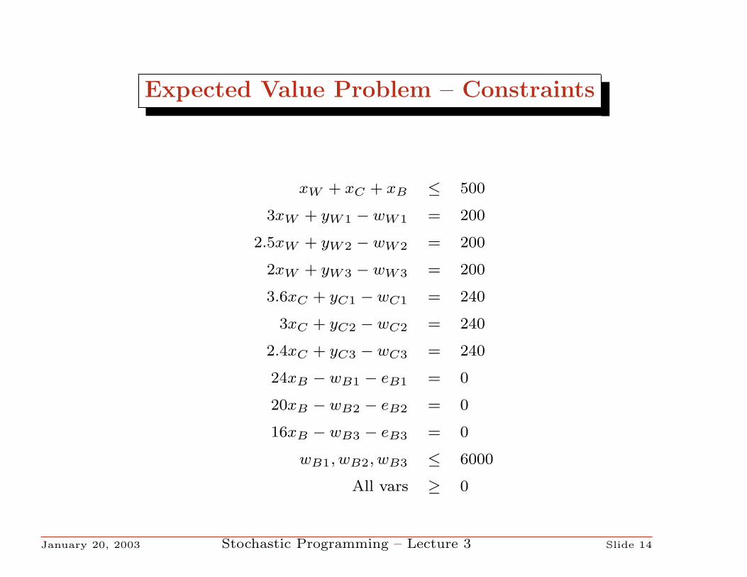
Expected Value Problem – Constraints

xW + xC + xB ≤ 500

3xW + yW1 − wW1 = 200

2.5xW + yW2 − wW2 = 200

2xW + yW3 − wW3 = 200

3.6xC + yC1 − wC1 = 240

3xC + yC2 − wC2 = 240

2.4xC + yC3 − wC3 = 240

24xB − wB1 − eB1 = 0

20xB − wB2 − eB2 = 0

16xB − wB3 − eB3 = 0

wB1, wB2, wB3 ≤ 6000

All vars ≥ 0


Optimal Solution

Wheat Corn Beans

s Plant (acres) 100 25 375

1 Production 510 288 6000

1 Sales 310 48 6000

1 Purchase 0 0 0


2 Sales 225 0 5000

2 Purchase 0 0 0


3 Sales 140 0 4000

3 Purchase 0 48 0

• (Expected) Profit: $108390


DE

• Congratulations, we’ve just solved our first stochastic program.

• What we’ve done is known as forming (and solving) thedeterministic equivalent of a stochastic program

• Note that you can always do this when...

¦ Ω is a finite set. (There are a finite number of scenariosω1, ω2, . . . ωK ∈ Ω)

¦ We are interested in optimizing an expected value.

⇒ We can write Eωf(x, ω) as∑K

k=1 pkf(x, ωk)


Wait and See

• Recall from last time, that Farmer Ted also “ran somescenarios”

• Given that he knew the yields, what was his best policy?

¦ We called these “Wait-and-see” solutions

0.8Y Y 1.2Y

Corn 25 80 66.67

Wheat 100 120 183.33

Beans 375 300 250

Profit 59950 118600 167667


Fortune Tellers

• Suppose Farmer Ted could with certainty tell whether or notthe upcoming growing season was going to be wet, average, ordry (or what his yields were going to be).

¦ His bursitits was acting up

¦ Consulting the Farmer’s Almanac

¦ Hiring a fortune teller

• The real point here is how much Farmer Ted would be willingto pay for this “perfect” information.

? In real-life problems, how much is it “worth” to invest in betterforecasting technology?

• This amount is called The Expected Value of PerfectInformation.


What is the EVPI?

• With perfect information, Farmer Ted’s Long Run Profit/Yearwould be:

¦ (1/3)(167667) + (1/3)(118600) + (1/3)(59950) = 115406

• Without perfect information, Farmer Ted can at best maximizehis expected profit by solving the stochastic program.

• In this case, he would make 108390 in the long run

? EVPI = 115406 - 108390 = 7016.

• Is there any other important information that you would like toknow?

¦ What is the value of including the randomess?


The Value of the Stochastic Solution (VSS)

• Suppose we just replaced the “random” quantities (the yields)by their mean values and solved that problem.

? Would we get the same expected value for the Farmer’s profit?

• How can we check?

¦ Solve the “mean-value” problem to get a first stage solutionx. (A “policy”).

¦ Fix the first stage solution at that value x, and solve all thescenarios to see Farmer Ted’s profit in each.

¦ Take the weighted (by probability) average of the optimalobjective value for each scenario


AMPL, Everyone?

• To do this, we’ll use AMPL

• You are welcome to solve problems anyway you can

¦ Except for copying/cheating

? An algebraic modeling language will be quite useful!

• Average AMPL proficiency was around 7, and minimium was3, so I am going to assume everyone comfortable with AMPL.

• There are some AMPL pointers on the web page.

• I have one copy of the AMPL book I can loan out for briefperiods.

• AMPL is all about algebraic notation, so lets convert FarmerTed to a more algebraic description...


Algebraic FT

• Sets...

¦ C : Set of crops

¦ D ⊆ C : Set of crops that have quotas

¦ Q ⊆ C : Set of crops that FT can purchase.

• Variables...

¦ xc, c ∈ C : Acres to allocate to c

¦ wc, c ∈ C : Amount of c to sell (at high price)

¦ yc, c ∈ C : (yc = 0 ∀ c ∈ C \Q) : Amount of c to purchase

¦ ec, c ∈ C : (ec = 0 ∀ c ∈ D) : Amount of c to sell (at lowprice)


AMPL

(Showing off AMPL here)


Great, but This Class is called Stochastic Programming

• Here’s how to create the deterministic equivalent...

• For each possible state of nature (scenario), formulate anappropriate LP model

• Combine these submodels into one “supermodel” making sure

¦ The first-stage variables are common to all submodels

¦ The second-stage variables in a submodel appear only inthat submodel

? Do this by attaching a “scenario index” to the second stagevariables and to the parameters that change in the differentscenarios


Deterministic Equivalent

• Combine these submodels into one “supermodel” making sure

¦ The first-stage variables are common to all submodels

¦ The second-stage variables in a submodel appear only inthat submodel

xW + xC + xB ≤ 500

3xW + yW1 − wW1 = 200

2.5xW + yW2 − wW2 = 200

2xW + yW3 − wW3 = 200


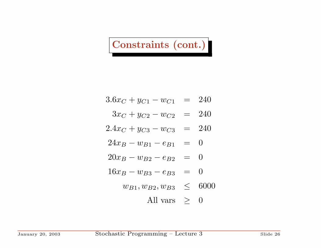
Constraints (cont.)

3.6xC + yC1 − wC1 = 240

3xC + yC2 − wC2 = 240

2.4xC + yC3 − wC3 = 240

24xB − wB1 − eB1 = 0

20xB − wB2 − eB2 = 0

16xB − wB3 − eB3 = 0

wB1, wB2, wB3 ≤ 6000

All vars ≥ 0


Computing Farmer Ted’s VSS

• Solve the “mean-value” problem to get a first stage solution x.(A “policy”).

¦ Mean yields Y = (2.5, 3, 20)

¦ (We already solved this problem).

¦ xW = 120, xC = 80, xB = 300

• Fix the first stage solution at that value x, and solve all thescenarios to see Farmer Ted’s profit in each.

• Take the weighted (by probability) average of the optimalobjective value for each scenario


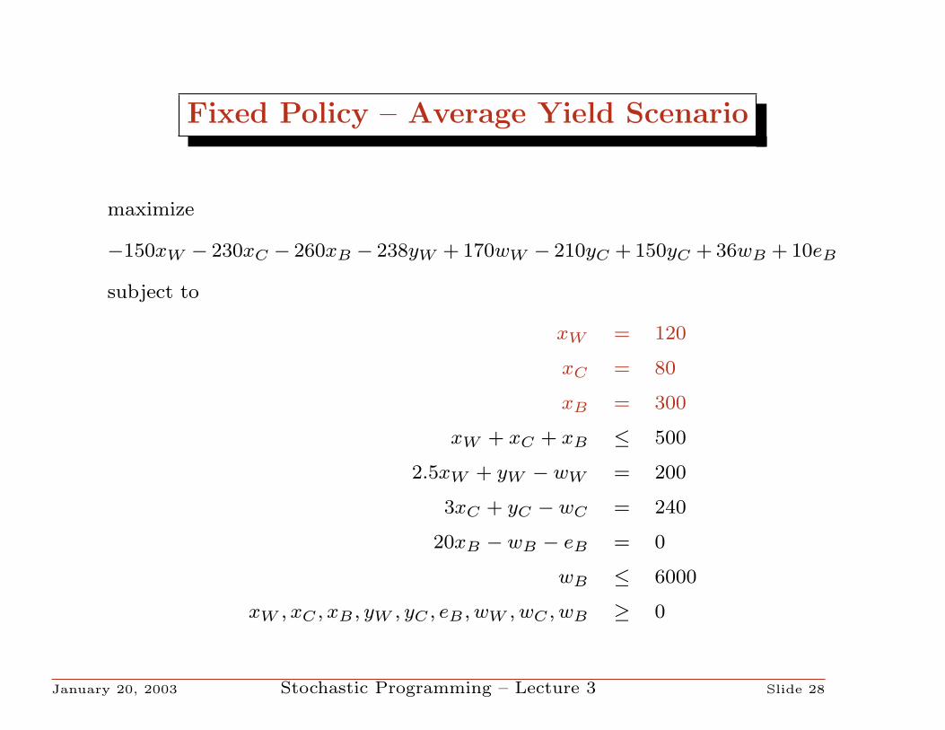
Fixed Policy – Average Yield Scenario

maximize

−150xW − 230xC − 260xB − 238yW + 170wW − 210yC + 150yC + 36wB + 10eB

subject to

xW = 120

xC = 80

xB = 300

xW + xC + xB ≤ 500

2.5xW + yW − wW = 200

3xC + yC − wC = 240

20xB − wB − eB = 0

wB ≤ 6000



Fixed Policy – Bad Yield Scenario

maximize


subject to

xW = 120

xC = 80

xB = 300

xW + xC + xB ≤ 500

2xW + yW − wW = 200

2.4xC + yC − wC = 240

16xB − wB − eB = 0

wB ≤ 6000



Fixed Policy – Good Yield Scenario

maximize


subject to

xW = 120

xC = 80

xB = 300

xW + xC + xB ≤ 500

3xW + yW − wW = 200

3.6xC + yC − wC = 240

24xB − wB − eB = 0

wB ≤ 6000



Profits

• If you solved those three problems, you would get

Yield Profit

Average 118600

Bad 55120

Good 148000

? Another trick – you don’t need to solve all three. Just solve theDE with the first stage fixed.

• I’ll show you this if we have time.


What’s it Worth to Model Randomness?

• If Farmer Ted implemented the policy based on using only“average” yields, he would plant xW = 120, xC = 80, xB = 300

• He would expect in the long run to make an average profit of...

¦ 1/3(118600) + 1/3(55120) + 1/3(148000) = 107240

• If Farmer Ted implemented the policy based on the solution tothe stochastic programming problem, he would plantxW = 170, xC = 80, xB = 250.

¦ From this he would expect to make 108390


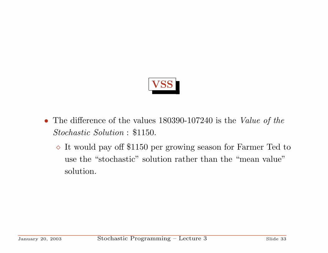
VSS

• The difference of the values 180390-107240 is the Value of theStochastic Solution : $1150.

¦ It would pay off $1150 per growing season for Farmer Ted touse the “stochastic” solution rather than the “mean value”solution.


stochastic programming modeling - cae...

Documents