stochastic optimization solution methods · basic idea l -shaped algorithm optimality cuts...

The L -Shaped MethodRegularized Decomposition

The Piecewise Quadratic Form of the L -shaped MethodsBunching and Other Efficiencies

Stochastic OptimizationSolution Methods

Alireza Ghaffari-Hadigheh

Azarbaijan Shahid Madani University (ASMU)

[email protected]

Fall 2017

Alireza Ghaffari-Hadigheh Stochastic Optimization



Overview

1 The L -Shaped MethodBasic IdeaL -Shaped AlgorithmOptimality CutsFeasibility cutsThe multicut version

2 Regularized DecompositionThe Regularized Decomposition Algorithm

3 The Piecewise Quadratic Form of the L -shaped MethodsAssumptionsExamplesAn Algorithm

4 Bunching and Other EfficienciesFull decomposabilityBunching




Basic IdeaL -Shaped AlgorithmOptimality CutsFeasibility cutsThe multicut version

Basic Idea

Basic two-stage stochastic linear program

min z = cT x +Q(x)s.t. Ax = b

x ≥ 0,(1)

Q(x) = EξQ(x , ξ(ω))

Q(x , ξ(ω)) = miny{q(ω)T y |Wy = h(ω)− T (ω)x , y ≥ 0}.The nonlinear objective term involves a solution of allsecond-stage recourse linear programs, we want to avoidnumerous function evaluations for it.

The basic idea: To approximate the nonlinear term in theobjective.

A master problem in x ,

Evaluate the recourse function exactly as a subproblem.





Assumption

The random vector ξ has finite support.k = 1, . . . ,K index its possible realizationspk are their probabilities.

The deterministic equivalent program

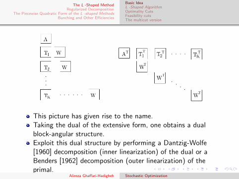
Associate one set of second-stage decisions, say, yk , to eachrealization ξ , i.e., to each realization of qk , hk , and Tk .Extensive form ( EF )

min z = cT x +∑K

k=1 pkqTk yk

s.t. Ax = bTkx + Wyk = hk , k = 1, . . . ,Kx ≥ 0, yk ≥ 0, k = 1, . . . ,K

(2)





This picture has given rise to the name.Taking the dual of the extensive form, one obtains a dualblock-angular structure.Exploit this dual structure by performing a Dantzig-Wolfe[1960] decomposition (inner linearization) of the dual or aBenders [1962] decomposition (outer linearization) of theprimal.





L -Shaped Algorithm

Step 0 Set r = s = ν = 0.

Step 1 Set ν = ν + 1 . Solve

min z = cT x + θ (3)

s.t. Ax = b,

D`x ≥ d`, ` = 1, . . . , r , (4)

E`x + θ ≥ e`, ` = 1, . . . , s, (5)

x ≥ 0, θ ∈ R.

Let (xν , θν) be an optimal solution.If no constraint (5) is presented, θν is set equal to−∞ and is not considered in the computation of xν .

Step 2 Check if x ∈ K2 If not, add at least one cut (4) andreturn to Step 1. Otherwise, go to Step 3.





L -Shaped Algorithm

Step 3 For k = 1, . . . ,K solve the linear program

min w = qTk ys.t. Wy = hk − Tkx

ν ,y ≥ 0

(6)

Let πνk be the simplex multipliers associated with theoptimal solution of Problem k of type (6). Define

Es+1 =k∑

k=1

pk � (πνk )TTk . (7)

es+1 =K∑

k=1

pk .(πνk )Thk . (8)

Let wν = es+1 − Es+1xν . If θν ≥ wν , stop; xν is an

optimal solution. Otherwise, set s = s + 1 , add to theconstraint set (5), and return to Step 1.





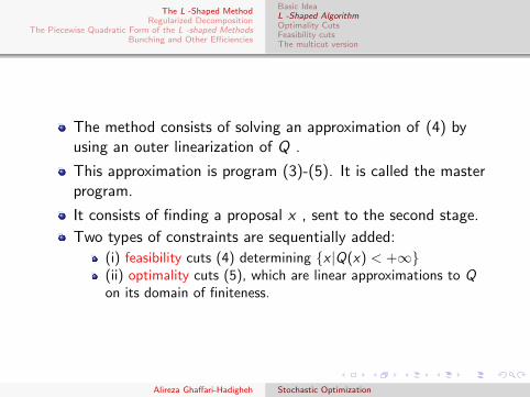
The method consists of solving an approximation of (4) byusing an outer linearization of Q .

This approximation is program (3)-(5). It is called the masterprogram.

It consists of finding a proposal x , sent to the second stage.

Two types of constraints are sequentially added:

(i) feasibility cuts (4) determining {x |Q(x) < +∞}(ii) optimality cuts (5), which are linear approximations to Qon its domain of finiteness.





Optimality cuts

Example

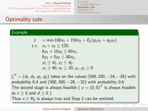
z = min 100x1 + 150x2 + Eξ(q1y1 + q2y2)s.t. x1 + x2 ≤ 120,

6y1 + 10y2 ≤ 60x1,8y1 + 5y2 ≤ 80x2,y1 ≤ d1, y2 ≤ d2,x1 ≥ 40, x2 ≥ 20, y1, y2 ≥ 0

ξT = (d1, d2, q1, q2) takes on the values (500, 100,−24,−28) withprobability 0.4 and (300, 300,−28,−32) with probability 0.6The second stage is always feasible ( y = (0, 0)T is always feasibleas x ≥ 0 and d ≥ 0 ).Thus x ∈ K2 is always true and Step 2 can be omitted.





Solution

Iteration 1:

Step 1 Ignoring θ , the master program is z =min{100x1 + 150x2|x1 + x2 ≤ 120, x1 ≥ 40, x2 ≥ 20}with solution x1 = (40, 20)T and θ1 = −∞.

Step 3 I For ξ = ξ1 , solve the programw = min{−24y1 − 28y2|6y1 + 10y2 ≤ 2400 ,8y1 + 5y2 ≤ 1600, 0 ≤ y1 ≤ 500, 0 ≤ y2 ≤ 100} .The solution is w1 = −6100,yT = (137.5, 100), πT1 = (0,−3, 0,−13) .I For ξ = ξ2 , solve the programw = min{−28y1 − 32y2|6y1 + 10y2 ≤ 2400,8y1 + 5y2 ≤ 1600, 0 ≤ y1 ≤ 300, 0 ≤ y2 ≤ 300} .The solution is w2 = −8384 ,yT = (80, 192), πT2 = (−2.32,−1.76, 0, 0) .





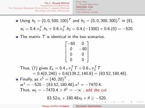
Using h1 = (0, 0, 500, 100)T and h2 = (0, 0, 300, 300)T in (8),

e1 = 0.4.πT1 .h1 + 0.6.πT2 .h2 = 0.4.(−1300) + 0.6.(0) = −520.

The matrix T is identical in the two scenarios.−60 0

0 −800 00 0

Thus, (7) gives E1 = 0.4 � πT1 T + 0.6 � πT2 T

= 0.4(0, 240) + 0.6(139.2, 140.8) = (83.52, 180.48).

Finally, as x1 = (40, 20)T ,w1 = −520− (83.52, 180.48).x1 = −7470.4.Thus, w1 = −7470.4 > θ1 = −∞ , add the cut

83.52x1 + 180.48x2 + θ ≥ −520.





Iteration 2:

Step 1 . Solve z = min{100x1 + 150x2 + θ|x1 + x2 ≤ 120,x1 ≥ 40, x2 ≥ 20, 83.52x1 + 180.48x2 + θ ≥ −520}with solutionz = −2299.2, x2 = (40, 80)T , θ2 = −18299.2 .

Step 3 I For ξ = ξ1 the programw = min{−24y1 − 28y2|6y1 + 10y2 ≤ 2400,8y1 + 5y2 ≤ 6400, 0 ≤ y1 ≤ 500, 0 ≤ y2 ≤ 100}has solution w1 = −9600,yT = (400, 0), πT1 = (−4, 0, 0, 0)T .I For ξ = ξ2 the programw = min{−28y1 − 32y2|6y1 + 10y2 ≤ 2400,8y1 + 5y2 ≤ 6400, 0 ≤ y1 ≤ 300, 0 ≤ y2 ≤ 300}has solution: w2 = −10320, yT = (300, 60), πT2 =(−3.2, 0,−8.8, 0) .





Apply (7) and (8),

e1 = 0.4.(0) + 0.6.(−2640) = −1584.

E1 = 0.4 � (240, 0) + 0.6 � (192, 0) = (211.2, 0).

As w2 = −1584− 211.2× 40 = −10032 > −18299.2,add the cut 211.2x1 + θ ≥ −1584.

Iteration 3:

Step 1 Master program has solution z = −1039.375 ,x3 = (66.828, 53.172)T , θ3 = −15697.994 .

Step 3 Add the cut 115.2x1 + 96x2 + θ ≥ −2104.

Iteration 4:

Step 1 Master program has solution z = −889.5,x4 = (40, 33.75)T , θ4 = −9952.

Step 3 The second-stage program for ξ = ξ2 has multiplesolutions. Selecting one of them, add the cut133.44x1 + 130.56x2 + θ ≥ 0





Iteration 5:

Step 1 Solve first stage programz = min{100x1 + 150x2 + θ|x1 + x2 ≤ 120, x1 ≥ 55, x2 ≥25, 83.52x1 + 180.48x2 + θ ≥ −520,211.2x1 + θ ≥ −1584, 115.2x1 + 96x2 + θ ≥ −2104,133.44x1 + 130.56x2 + θ ≥ 0}. It has solutionz = −855.833 , x5 = (46.667, 36.25)T , θ5 = −10960 .

Step 3 I For ξ = ξ1 the programw = min{−24y1 − 28y2|6y1 + 10y2 ≤ 2800,8y1 + 5y2 ≤ 2900, 0 ≤ y1 ≤ 500, 0 ≤ y2 ≤ 100}has the solution w1 = −10000 , yT = (300, 100) ,πT

1 = (0,−3, 0,−13) .I For ξ = ξ2 the programw = min{−28y1 − 32y2|6y1 + 10y2 ≤ 2800,8y1 + 5y2 ≤ 2900, 0 ≤ y1 ≤ 300, 0 ≤ y2 ≤ 300}has the solution w2 = −11600 , yT = (300, 100) ,πT

2 = (−2.32,−1.76, 0, 0).





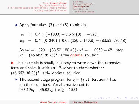
Apply formulaes (7) and (8) to obtain

e5 = 0.4× (−1300) + 0.6× (0) = −520,

E5 = 0.4 � (0, 240) + 0.6 � (139.2, 140.8) = (83.52, 180.48).

As w5 = −520− (83.52, 180.48) � x5 = −10960 = θ5 , stop.x5 = (46.667, 36.25)T is the optimal solution.

I This example is small, it is easy to write down the extensiveform and solve it with an LP-solver to check whether(46.667, 36.25)T is the optimal solution.

The second-stage program for ξ = ξ2 at Iteration 4 hasmultiple solutions. An alternative cut is165.12x1 + 46.08x2 + θ ≥ −1584.





Example

z = minEξ(y1 + y2)

s.t. 0 ≤ x ≤ 10,

y1 − y2 = ξ − x ,

y1, y2 ≥ 0,

ξ takes the values 1 , 2 and 4 with probability 13 each.

h = ξ , T = [1] and x are all scalars.

Step 2 can be omitted.





Iteration 1.Take x1 = 0 as starting point.

Step 3 I For ξ = ξ1 , solve the programw = min{y1 + y2|y1 − y2 = 1, y1, y2 ≥ 0}. Thesolution is w1 = 1 , yT = (1, 0) , π1 = (1) .I For ξ = ξ2 , solve the programw = min{y1 + y2|y1 − y2 = 2, y1, y2 ≥ 0}. Thesolution is w2 = 2 , yT = (2, 0) , π2 = (1).I For ξ = ξ3 , solve the programw = min{y1 + y2|y1 − y2 = 4, y1, y2 ≥ 0}. Thesolution is w3 = 4 , yT = (4, 0) , π3 = (1).I Using hk = ξk , one obtainse1 = 1

3 � 1 � (1 + 2 + 4) = 73 . Formula (7) gives

E1 = 13 � 1 � (1 + 1 + 1) = 1 . Finally, as x1 = (0) ,

w1 = 73 > −∞ ; add the cut, θ ≥ 7

3 − x .





Iteration 2:

Step 1 x2 = 10 ,

Step 3 . x2 is not optimal; add the cut θ ≥ x − 73

Iteration 3:

Step 1 x3 = 73 ,

Step 3 . x3 is not optimal; add the cut θ ≥ x−13

Iteration 4:

Step 1 x4 = 1.5 ,

Step 3 . x4 is not optimal; add the cut θ ≥ 5−x3

Iteration 5:

Step 1 x5 = 2 ,

Step 3 . x5 is optimal.





These cuts are supporting hyperplanes of Q(x) .

Q(x) = EξQ(x , ξ) =K∑

k=1

pkQ(x , ξk) ,

Q(x , ξ) = min{y1 + y2|y1 − y2 = ξ − x , y1, y2 ≥ 0} .

If x ≤ ξ , the second-stage optimalsolution is yT = (ξ − x , 0) andyT = (0, x − ξ) if x ≥ ξ.

Q(x , ξ) =

{ξ − x if x ≤ ξ,x − ξ if x ≥ ξ.





Consider Iteration 1. x1 = 0 is the starting point.

Step 3 obtains the cut θ ≥ 73 − x .

For x = x1 , Q(x , 1) = 1,Q(x , 2) = 2,Q(x , 4) = 4 andQ(x) = 7

3 .

Around x = x1 ,Q(x , 1) = 1− x ,Q(x , 2) = 2− x ,Q(x , 4) = 4− x andQ(x) = 7

3 − x .

Around x = x1 is simply 0 ≤ x ≤ 1 .

This can be seen from the construction of Q(x , 1) whereQ(x , 1) changes when x = 1 .

In general, such a range can be obtained by linearprogramming sensitivity analysis around the second stageoptimal solutions.

We conclude that Q(x) = 73 − x within 0 ≤ x ≤ 1 .

The optimality cut at the end of Iteration 1 is θ ≥ 73 − x





Step 2 of the L-shaped method consists of determining whether afirst-stage decision x ∈ K1 is also second stage feasible, i.e. x ∈ K2.

Step 2 For k = 1, . . . ,K solve the linear program

minw ′ = eTν+ + eTν− (9)

s.t. Wy + Iν+ − Iν− = hk − Tkxν , (10)

y ≥ 0, ν+ ≥ 0, ν− ≥ 0,

eT = (1, . . . , 1) , until, for some k , the optimal value w ′ > 0

σν be the associated simplex multipliers

Define

Dr+1 = (σν)TTk (11)

dr+1 = (σν)Thk (12)

Set r = r + 1 , add to the constraint set (4), and return to Step 1.If for all k , w ′ = 0 , go to Step 3.





Example

min 3x1 + 2x2 − Eξ(15y1 + 12y2)

s.t. 3y1 + 2y2 ≤ x1,

2y1 + 5y2 ≤ x2,

0.8ξ1 ≤ y1 ≤ ξ1,

0.8ξ2 ≤ y2 ≤ ξ2,

x , y ≥ 0, a.s.,

I ξ1 = 4 or 6 and ξ2 = 4 or 8 , independently, with probability 12

each and ξ = (ξ1, ξ2)T .

To keep the discussion short, assume the first consideredrealization of ξ is (6, 8)T .





Starting from an initial solution x1 = (0, 0)T , Program (9)-(10)reads as follows

w ′ = min ν+1 + ν−1 + ν+

2 + ν−2 + ν+3 + ν−3

+ν+4 + ν−4 + ν+

5 + ν−5 + ν+6 + ν−6

s.t. ν+1 − ν

−1 + 3y1 + 2y2 ≤ 0,

ν+2 − ν

−2 + 2y1 + 5y2 ≤ 0,

ν+3 − ν

−3 + y1 ≥ 4.8,

ν+4 − ν

−4 + y2 ≥ 6.4,

ν+5 − ν

−5 + y1 ≤ 6,

ν+6 − ν

−6 + y2 ≤ 8,

ν+, ν−, y ≥ 0





The optimal solution is w ′ = 11.2 with non-zero variablesν+

3 = 4.8 and ν+4 = 6.4 .

The dual variables are σ1 = (−3/11,−1/11, 1, 1, 0, 0).

h = (0, 0, 4.8, 6.4, 6, 8)T and T consists of the two columns(−1, 0, 0, 0, 0, 0)T and (0,−1, 0, 0, 0, 0)T .

Thus, D1 = (−0.273,−0.091, 1, 1, 0, 0) � T = (0.273, 0.091) ,and d1 = (−0.273,−0.091, 1, 1, 0, 0) � h = 11.2 , creating thefeasibility cut 3

11x1 + 111x2 ≥ 11.2 or 3x1 + x2 ≥ 123.2 .

The first-stage solution is then x2 = (41.067, 0)T .

A second feasibility cut is x2 ≥ 22.4.

The first-stage solution becomes x3 = (33.6, 22.4)T .

A third feasibility cut x2 ≥ 41.6 is generated.

The first-stage solution is: x4 = (27.2, 41.6)T , which yieldsfeasible second-stage decisions.





In some cases, Step 2 can be simplified.

When the second stage is always feasible. The stochastic program isthen said to have complete recourse.

When it is possible to derive some constraints that have to besatisfied to guarantee second-stage feasibility. These constraints aresometimes called induced constraints. They can be obtained from agood understanding of the model.

When Step 2 is not required for all k = 1, . . . ,K , but for one hk .

Theorem

When ξ is a finite random variable, the L -shaped algorithm finitelyconverges to an optimal solution when it exists or proves the infeasibilityof Problem

min cT x +Q(x)

s.t. x ∈ K1 ∩ K2.





In Step 3 of the L -shaped method, all K realizations of thesecond-stage program are optimized to obtain their optimalsimplex multipliers.

These multipliers are aggregated in (11) and (12) to generateone cut (5).

In the multicut version, one cut per realization in the secondstage is placed.

Adding multiple cuts at each iteration corresponds toincluding several columns in the master program of an innerlinearization algorithm.





The Multicut L -Shaped Algorithm

Step 0 . Set r = ν = 0 and sk = 0 for all k = 1, . . . ,K .

Step 1 Set ν = ν + 1 . Solve the linear program (13)-(16):

min z = cT x +K∑

k=1

θk (13)

s.t. Ax = b, (14)

D`x ≥ d`, ` = 1, . . . , r , (15)

E`(k)x + θk ≥ e`(k), `(k) = 1, . . . , sk , (16)

x ≥ 0, k = 1, . . . ,K ,

Let (xν , θν1 , . . . , θνK ) be an optimal solution of (13)-(16). If no constraint

(16) is presented for some k , θνk is set equal to −∞ and is notconsidered in the computation of xν .





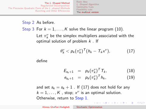
Step 2 As before.

Step 3 For k = 1, . . . ,K solve the linear program (10).

Let πνk be the simplex multipliers associated with theoptimal solution of problem k . If

θνk < pk(πνk )T (hk − Tkxν), (17)

define

Esk+1 = pk(πνk )TTk , (18)

esk+1 = pk(πνk )Thk , (19)

and set sk = sk + 1 . If (17) does not hold for anyk = 1, . . . ,K , stop; xν is an optimal solution.Otherwise, return to Step 1.





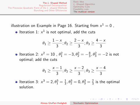
illustration on Example in Page 16. Starting from x1 = 0 ,

Iteration 1: x1 is not optimal, add the cuts

θ1 ≥1− x

3; θ2 ≥

2− x

3; θ3 ≥

4− x

3

Iteration 2: x2 = 10 , θ21 = −3, θ2

2 = −83 , θ

23 = −2 is not

optimal; add the cuts

θ1 ≥x − 1

3; θ2 ≥

x − 2

3; θ3 ≥

x − 4

3

Iteration 3: x3 = 2, θ31 = 1

3 , θ32 = 0, θ3

3 = 23 is the optimal

solution.




The Regularized Decomposition Algorithm

Regularized decomposition is a method that combines amulticut approach for the representation of the second-stagevalue function with the inclusion in the objective of aquadratic regularizing term.

This additional term is included to avoid two classicaldrawbacks of the cutting plane methods.

Initial iterations are often inefficient.Iterations may become degenerate at the end of the process.






Step 0 Set r = ν = 0, sk = 0 for all k = 1, . . . ,K . Select a1 afeasible solution.

Step 1 Set ν = ν + 1 . Solve the regularized master program

min cT x +k∑

k=1

θk +1

2‖x − aν‖2 (20)

s.t. Ax = b,

D`x ≥ d`, ` = 1, . . . , r ,

E`(k)x + θk ≥ e`(k), `(k) = 1, . . . , sk , k = 1, . . . ,K ,

x ≥ 0.

Let (xν , θν) be an optimal solution to (20) where (θν)T = (θν1 , . . . , θνK )T

. If sk = 0 for some k , θνk is ignored in the computation. IfcT xν + eT θν = cTaν +Q(aν) , stop; aν is optimal.





Step 2 As before, if a feasibility cut (4) is generated, setaν+1 = aν (null infeasible step), and go to Step 1.

Step 3 For k = 1, . . . ,K , solve the linear subproblem (10).Compute Qk(xν) . If (17) holds, add an optimalitycut (16) using formulas (18) and (19). Setsk = sk + 1 .

Step 4 If (17) does not hold for any k , then aν+1 = xν

(exact serious step); go to Step 1.

Step 5 . If cT xν +Q(xν) ≤ cTaν +Q(aν) , then aν+1 = xν

(approximate serious step); go to Step 1. Else,aν+1 = aν (null feasible step), go to Step 1.

When a serious step is made, the value Q(aν+1) should bememorized, so that no extra computation is needed in Step 1 forthe test of optimality.





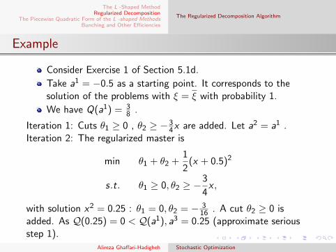
Example

Consider Exercise 1 of Section 5.1d.

Take a1 = −0.5 as a starting point. It corresponds to thesolution of the problems with ξ = ξ with probability 1.

We have Q(a1) = 38 .

Iteration 1: Cuts θ1 ≥ 0 , θ2 ≥ −34x are added. Let a2 = a1 .

Iteration 2: The regularized master is

min θ1 + θ2 +1

2(x + 0.5)2

s.t. θ1 ≥ 0, θ2 ≥ −3

4x ,

with solution x2 = 0.25 : θ1 = 0, θ2 = − 316 . A cut θ2 ≥ 0 is

added. As Q(0.25) = 0 < Q(a1), a3 = 0.25 (approximate seriousstep 1).





Iteration 3: The regularized master is

min θ1 + θ2 +1

2(x − 0.25)2

s.t. θ1 ≥ 0, θ2 ≥ −3

4x , θ2 ≥ 0,

with solution x3 = 0.25, θ1 = 0 , θ2 = 0 . Because θν = Q(aν) , asolution is found.




AssumptionsExamplesAn Algorithm

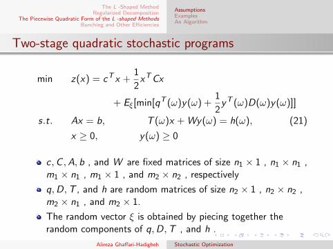
Two-stage quadratic stochastic programs

min z(x) = cT x +1

2xTCx

+ Eξ[min[qT (ω)y(ω) +1

2yT (ω)D(ω)y(ω)]]

s.t. Ax = b, T (ω)x + Wy(ω) = h(ω), (21)

x ≥ 0, y(ω) ≥ 0

c ,C ,A, b , and W are fixed matrices of size n1 × 1 , n1 × n1 ,m1 × n1 , m1 × 1 , and m2 × n2 , respectively

q,D,T , and h are random matrices of size n2 × 1 , n2 × n2 ,m2 × n1 , and m2 × 1.

The random vector ξ is obtained by piecing together therandom components of q,D,T , and h .





Assumption 1

The random vector ξ has a discrete distribution.

Assumption 2

The matrix C is positive semi-definite and the matrices D(ω) are positivesemi-definite for all ω . The matrix W has full row rank.

The first assumption guarantees the existence of a finitedecomposition of the second-stage feasibility set K2 .

The second assumption guarantees that the recourse functions areconvex and well-defined.

Recourse function for a given ξ(ω)

Q(x , ξ(ω)) = min{qT (ω)y(ω) +1

2yT (ω)D(ω)y(ω)|

T (ω)x + Wy(ω) = h(ω), y(ω) ≥ 0}, (22)





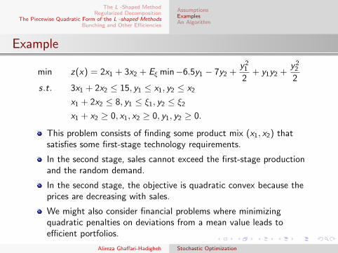
Example

min z(x) = 2x1 + 3x2 + Eξ min−6.5y1 − 7y2 +y2

1

2+ y1y2 +

y22

2s.t. 3x1 + 2x2 ≤ 15, y1 ≤ x1, y2 ≤ x2

x1 + 2x2 ≤ 8, y1 ≤ ξ1, y2 ≤ ξ2

x1 + x2 ≥ 0, x1, x2 ≥ 0, y1, y2 ≥ 0.

This problem consists of finding some product mix (x1, x2) thatsatisfies some first-stage technology requirements.

In the second stage, sales cannot exceed the first-stage productionand the random demand.

In the second stage, the objective is quadratic convex because theprices are decreasing with sales.

We might also consider financial problems where minimizingquadratic penalties on deviations from a mean value leads toefficient portfolios.





ξ1 can take the three values 2, 4, and 6 with probability 13 ,

ξ2 can take the values 1, 3, and 5 with probability 13 ,

ξ1 and ξ2 are independent of each other.

For very small values of x1 and x2 , it always is optimal in thesecond stage to sell the production, y1 = x1 and y2 = x2 .0 ≤ x1 ≤ 2 and 0 ≤ x2 ≤ 1, y1 = x1, y2 = x2 is the optimalsolution of the second stage for all ξ .

If needed, the reader may check this using theKarush-Kuhn-Tucker conditions.

Q(x , ξ) = −6.5x1 − 7x2 +x2

12 + x1x2 +

x222 for all ξ and

Q(x) = −6.5x1 − 7x2 +x2

12 + x1x2 +

x222 .

Here, the cell is {(x1, x2)|0 ≤ x1 ≤ 2, 0 ≤ x2 ≤ 1} . Withinthat cell, Q(x) is quadratic.





Definition

A finite closed convex complex K is a finite collection of closedconvex sets, called the cells of K , such that the intersection of twodistinct cells has an empty interior.

Definition

A piecewise convex program is a convex program of the forminf{z(x)|x ∈ S} where f is a convex function on Rn and S is aclosed convex subset of the effective domain of f with nonemptyinterior.The region where f is finite is called the effective domain of f(dom f ).





Assumption

Let K be a finite closed convex complex such that

(a) the n -dimensional cells of K cover S ,

(b) either f is identically −∞ or for each cell Cν of thecomplex there exists a convex function zν(x) definedon S and continuously differentiable on an open setcontaining Cν which satisfies

z(x) = zν(x)∀x ∈ Cν ,∇zν(x) ∈ ∂z(x)∀x ∈ Cν .

Definition

A piecewise quadratic function is a piecewise convex functionwhere on each cell Cν the function zν is a quadratic form.





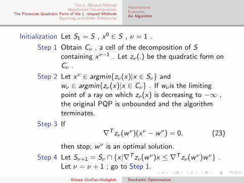
Initialization Let S1 = S , x0 ∈ S , ν = 1 .

Step 1 Obtain Cν , a cell of the decomposition of Scontaining xν−1 . Let zν(.) be the quadratic form onCν .

Step 2 Let xν ∈ argmin{zν(x)|x ∈ Sν} andwν ∈ argmin{zν(x)|x ∈ Cν} . If wν is the limitingpoint of a ray on which zν(x) is decreasing to −∞ ,the original PQP is unbounded and the algorithmterminates.

Step 3 If∇T zν(wν)(xν − wν) = 0, (23)

then stop; wν is an optimal solution.

Step 4 Let Sν+1 = Sν ∩ {x |∇T zν(wν)x ≤ ∇T zν(wν)wν} .Let ν = ν + 1 ; go to Step 1.




Full decomposabilityBunching

One big issue in the efficient implementation of the L -shapedmethod is in Step 3.The second-stage program (6) has to be solved K times toobtain the optimal multipliers, πνk .For a given xν and a given realization k , let B be the optimalbasis of the second stage.It is well-known from linear programming that B is a squaresubmatrix of W such that(πνk )T = qTk,BB

−1, qT − (πνk )TW ≥ 0,B−1(hk − Tkxν) ≥ 0 ,

where qk,B denotes the restriction of qk to the selection ofcolumns that define B .Important savings can be obtained in Step 3 when the samebasis B is optimal for several realizations of k .This is especially the case when q is deterministic.Then, two different realizations that share the same basis alsoshare the same multipliers πνk .





assumptions

q is deterministic.

Define the set of possible right-hand sides in the second stage.

τ = {t|t = hk − Tkxν for some k = 1, . . . ,K} (24)

Let B be a square submatrix and πT = qTBB−1 .

B satisfies the optimality criterion qT − πTW ≥ 0 .

Define a bunch as

Bu = {t ∈ τ |B−1t ≥ 0} (25)

the set of possible right-hand sides that satisfy the feasibilitycondition.

Thus, π is an optimal dual multiplier for all t ∈ Bu .

By virtue of Step 2 of the L -shaped method, only feasiblefirst-stage xν ∈ K2 are considered.

By construction, τ ⊆ posW = {t|t = Wy , y ≥ 0} .





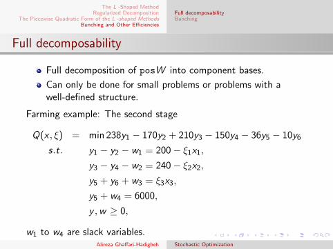
Full decomposability

Full decomposition of posW into component bases.

Can only be done for small problems or problems with awell-defined structure.

Farming example: The second stage

Q(x , ξ) = min 238y1 − 170y2 + 210y3 − 150y4 − 36y5 − 10y6

s.t. y1 − y2 − w1 = 200− ξ1x1,

y3 − y4 − w2 = 240− ξ2x2,

y5 + y6 + w3 = ξ3x3,

y5 + w4 = 6000,

y ,w ≥ 0,

w1 to w4 are slack variables.Alireza Ghaffari-Hadigheh Stochastic Optimization




This second stage has complete recourse, so posW = R4.

The matrix

w =

1 −1 0 0 0 0 −1 0 0 00 0 1 0 0 0 0 −1 0 00 0 0 −1 1 1 0 0 1 00 0 0 0 1 0 0 0 0 1

Theoretically,

(104

)= 210 bases could be found.

w1,w2, and w3 are never in the basis, as they are alwaysdominated by y2, y4 , and y6, respectively.

y5 is always in the basis.

y1 or y2 and y3 or y4 are always basic.





not only is a full decomposition of posW available, but animmediate analytical expression for the multipliers is also obtained.

π1(ξ) =

{238 if ξ1x1 < 200,−170 otherwise

π2(ξ) =

{210 if ξ2x2 < 240,−150 otherwise

π3(ξ) =

{−36 if ξ3x3 < 6000,

0 otherwise

π4(ξ) =

{10 if ξ3x3 > 6000,0 otherwise

The decomposition is thus (1,3,5,6) , (1,3,5,10) , (1,4,5,6) ,(1,4,5,10) , (2,3,5,6) , (2,3,5,10) , (2,4,5,6) , (2,4,5,10),

The four variables in a basis are described by their indices (the indexis 6 + j for the j -th slack variable).





the set of possible right-hand sides in the second stage:τ = {t|t = hk − Tkx for some k = 1, . . . ,K}Consider some k . Denote tk = hk − Tkx .

Arbitrarily be k = 1 , or if available, a value of k such thathk − Tkx = t , the expectation of all tk ∈ τ .

Let B1 be the corresponding optimal basis and π(1) thecorresponding vector of simplex multipliers.

Then, Bu(1) = {t ∈ τ |B−11 t ≥ 0} . Let τ1 = τ\Bu(1) .

Repeat the same operations.

Some element of τ1 is chosen.

The corresponding optimal basis B2 and its associated vectorof multipliers π(2) are formed .

Then, Bu(2) = {t ∈ τ1|B−12 t ≥ 0} and τ2 = τ1\Bu(2) .

The process is repeated until all tk ∈ τ are in one of b totalbunches.





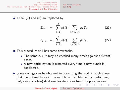
Then, (7) and (8) are replaced by

Es+1 =b∑`=1

π(`)T∑

tk∈Bu(`)

pkTk (26)

es+1 =b∑`=1

π(`)T∑

tk∈Bu(`)

pkhk (27)

This procedure still has some drawbacks.

The same tk ∈ τ may be checked many times against differentbases.A new optimization is restarted every time a new bunch isconsidered.

Some savings can be obtained in organizing the work in such a waythat the optimal basis in the next bunch is obtained by performingonly one (or a few) dual simplex iterations from the previous one.





Example

Consider the following second stage:

max 6y1 + 5y2 + 4y3 + 3y4

s.t. 2y1 + y2 + y3 ≤ ξ1,

y2 + y3 + y4 ≤ ξ2,

y1 + y3 ≤ x1,

2y2 + y4 ≤ x2

ξ1 ∈ {4, 5, 6, 7, 8} with equal probability 0.2 each

ξ2 ∈ {2, 3, 4, 5, 6} with equal probability 0.2 each





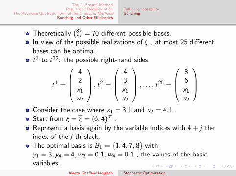
Theoretically(8

4

)= 70 different possible bases.

In view of the possible realizations of ξ , at most 25 differentbases can be optimal.

t1 to t25: the possible right-hand sides

t1 =

42x1

x2

, t2 =

43x1

x2

, . . . , t25 =

86x1

x2

Consider the case where x1 = 3.1 and x2 = 4.1 .

Start from ξ = ξ = (6, 4)T .

Represent a basis again by the variable indices with 4 + j theindex of the j th slack.

The optimal basis is B1 = {1, 4, 7, 8} withy1 = 3, y4 = 4,w3 = 0.1,w4 = 0.1 , the values of the basicvariables.





The optimal dictionary associated with B1

z = 3ξ1 + 3ξ2 − y2 − 2y3 − 3w1 − 3w2,

y1 =1

2ξ1 −

1

2y2 −

1

2y3 −

1

2w1,

y4 = ξ2 − y2 − y3 − w2,

w3 = 3.1− 1

2ξ1 +

1

2y2 −

1

2y3 +

1

2w1,

w4 = 4.1− ξ2 − y2 + y3 + w2.

This basis is optimal and feasible as long as ξ12 ≤ 3.1 and

ξ2 ≤ 4.1 , which in view of the possible values of ξ amountsto ξ1 ≤ 6 and ξ2 ≤ 4 , so thatBu(1) = {t1, t2, t3, t6, t7, t8, t11, t12, t13} .





Neighboring bases can be obtained by considering eitherξ1 ≥ 7 or ξ2 ≥ 5 .Let us start with ξ2 ≥ 5 .This means that w4 becomes negative and a dual simplexpivot is required in Row 4.This means that w4 leaves the basis, and, according to theusual dual simplex rule, y3 enters the basis.The new basis is B2 = {1, 3, 4, 7}

z = 3ξ1 + ξ2 + 8.2− 3y2 − 3w1 − w2 − 2w4,

y1 =ξ1

2− ξ2

2+ 2.05− y2 −

w1

2+

w2

2− w4

2,

y3 = ξ2 − 4.1 + y2 − w2 + w − 4,

y4 = 4.1− 2y2 − w − 4,

w3 = 5.15− ξ1

2− ξ2

2+

w1

2+

w2

2− w4

2.





The condition ξ1 − ξ2 + 4.1 ≥ 0 always holds.This basis is optimal as long as ξ2 ≥ 5 and ξ1 + ξ2 ≤ 10 ,So that Bu(2) = {t4, t5, t9} .Neighboring bases are B1 when ξ2 ≤ 4 and B3 obtained whenw3 < 0 , i.e., ξ1 + ξ2 ≥ 11 .This basis corresponds to w3 leaving the basis and w2 enteringthe basis.B1 = {1, 4, 7, 8} Bu(1) = {t1, t2, t3, t6, t7, t8, t11, t12, t13}B2 = {1, 3, 4, 7} Bu(2) = {t4, t5, t9}B3 = {1, 3, 4, 6} Bu(3) = {t10, t14, t15}B4 = {1, 4, 5, 6} Bu(4) = {t19, t20, t24, t25}B5 = {1, 2, 4, 5} Bu(5) = {t18, t22, t23}B6 = {1, 2, 4, 8} Bu(6) = {t16, t17, t21}B7 = {1, 2, 5, 8} Bu(7) = ∅.

Several paths are possible, as one may have chosen B6 instead ofB2 as a second basis.


stochastic optimization solution methods · basic idea l -shaped algorithm optimality cuts...

Documents