stochastic, dynamic, and periodic networked control...
TRANSCRIPT

UNIVERSIDADE TÉCNICA DE LISBOA
INSTITUTO SUPERIOR TÉCNICO
Stochastic, Dynamic, and PeriodicNetworked Control Systems
Duarte Jose Guerreiro Tome Antunes
Supervisor: Doctor Carlos Jorge Ferreira SilvestreCo-Supervisor: Doctor Joao Pedro Hespanha
Thesis approved in public session to obtain the PhD Degree inElectrical and Computer Engineering
Juri final classification: Pass with Distinction
JuriChairperson: Chairman of the IST Scientific Board
Members of the Committee:Doctor Wilhelmus Petrus Maria Hubertina HeemelsDoctor Joao Pedro HespanhaDoctor Fernando Manuel Ferreira Lobo PereiraDoctor Joao Manuel Lage de Miranda LemosDoctor Carlos Jorge Ferreira SilvestreDoctor Joao Manuel de Freitas Xavier
2011

ii
UNIVERSIDADE TECNICA DE LISBOA
INSTITUTO SUPERIOR TECNICO
Stochastic, Dynamic, and PeriodicNetworked Control Systems
Duarte Jose Guerreiro Tome Antunes
Supervisor: Doctor Carlos Jorge Ferreira SilvestreCo-Supervisor: Doctor Joao Pedro Hespanha
Thesis approved in public session to obtain the PhD Degree inElectrical and Computer Engineering
Juri final classification: Pass with Distinction
JuriChairperson: Chairman of the IST Scientific Board
Members of the Committee:Doctor Wilhelmus Petrus Maria Hubertina Heemels, Full Professor at
Technical University of EindhovenDoctor Joao Pedro Hespanha, Full Professor at
University of California, Santa BarbaraDoctor Fernando Manuel Ferreira Lobo Pereira, Full Professor at
Faculdade de Engenharia da Universidade do PortoDoctor Joao Manuel Lage de Miranda Lemos, Full Professor at
Instituto Superior TecnicoDoctor Carlos Jorge Ferreira Silvestre, Associate Professor at
Instituto Superior TecnicoDoctor Joao Manuel de Freitas Xavier, Assistant Professor at
Instituto Superior Tecnico
Funding Institutions:Fundacao para a Ciencia e a Tecnologia
2011

ii

Abstract
Networked Control Systems are controlled physical systems where sensing andcontrol devices are connected via communication networks. Motivated by theproliferation of embedded sensors, microprocessors, and wireless networks, ex-tensive research has been conducted in recent years on networked control sys-tems, bringing forth important theoretical advances in the automatic controlfield.
The results of the present thesis spring from networked control applications, con-sidering three di!erent network scenarios. First, considering a network modelinspired on the Ethernet and the Wireless 802.11 protocols, where delays andintervals between transmissions are stochastic, we provide a stability resultthat can be tested using the Nyquist criterion and show how to compute mo-ment Lyapunov exponents to investigate performance. In the same setup, butconsidering several asynchronous networks, we establish that stability can beasserted by computing the spectral radius of an integral operator. Second,assuming that all the sensing and control devices in the network can run anarbitration algorithm, we propose dynamic protocols, assigning priorities basedon data sent by the devices, which can outperform any static protocol wherenodes transmit in a prescribed order. Third, considering networks that guaran-tee fixed transmission rates, although in general di!erent among users-such ascircuit-switching networks-, we propose output regulation and gain-schedulingsolutions for multi-rate systems.
We use the framework of hybrid systems to model several networked controlscenarios, and the machinery of Volterra equations, piecewise deterministicprocesses, and dynamic programming to establish the main results of the thesis.These results are often stated with enough generality that their interest is shownto exceed the networked control systems scope.
Keywords: Networked Control Systems; Impulsive Systems; Stochastic Hy-brid Systems; Asynchronous Systems; Volterra Equations; Dynamic Protocols;Piecewise Deterministic Processes; Gain-Scheduling; Output Regulation; Multi-Rate Control.

iv

Resumo
Sistemas de controlo sobre redes são sistemas de controlo automático em quesensores, atuadores e controladores comunicam entre si através de redes decomunicação. A proliferação de sensores embebidos, micro-processadores e re-des de comunicação sem fios despertou o interesse por estes sistemas, o que setraduziu em progressos significativos na área do controlo automático.
Esta tese aborda problemas na área do controlo automático que provem de trêscenários para sistemas de controlo sobre redes. Em primeiro lugar, considera-se modelos para a rede inspirados na rede Ethernet e na rede Wireless 802.11,obtendo-se resultados de estabilidade que podem ser testados através do critériode Nyquist e mostrando-se também como se pode avaliar o desempenho dosistema. Ainda para este cenário, mas considerando várias redes operando ass-incronamente, prova-se que a estabilidade do sistema de controlo sobre redespode ser testada através do cálculo do raio espetral de um operador integral.Em segundo lugar, assumindo que os vários intervenientes na cadeia de con-trolo têm capacidade de processamento, propõem-se protocolos dinâmicos, queatribuem prioridades de acesso à rede com base na informação enviada pelosintervenientes na cadeia de controlo, conseguindo superar a performance dosprotocolos estáticos, em que uma dada ordem para as transmissões é repetidaperiodicamente. Em terceiro lugar, considera-se redes que garantem uma deter-minada taxa de transmissão, possivelmente diferente para cada utilizador-taiscomo as redes de circuitos comutados-, e propõem-se soluções para os problemasde regulação da saída e de síntese de sistemas de controlo de ganhos comutadospara sistemas multi-ritmo.
A capacidade de modelação dos sistemas híbridos e as ferramentas matemáticaspara equações de Volterra e de Fredholm, de processos determinísticos portroços, e de programação dinâmica estão na base dos principais resultados datese. Os resultados são enunciados com generalidade, o que permite mostrarque o seu interesse excede a área dos sistemas de controlo sobre redes.
Palavras Chave: Sistemas de controlo sobre redes; Sistemas Impulsivos; Sis-temas Híbridos Estocásticos; Sistemas Assíncronos; Multi-Ritmo; Equaçõesde Volterra; Protocolos Dinâmicos; Processos Determinísticos por Troços; Sis-temas de controlo de ganhos comutados; Regulação da Saída.

vi

Ad majorem Dei gloriam
“Àquele que puder ser sábio, não lhe perdoamos que o não seja”(Josemaria Escrivá).


AcknowledgementsFirst and foremost, I acknowledge the support and friendship of my two super-visors. I am grateful to Carlos Silvestre for several useful conversations. Histrust, especially in di"cult moments, has been invaluable. On the other hand,it has been an enormous pleasure to work with such an honest and dedicatedresearcher as Joao Hespanha. I am very grateful for his thorough work in ourarticles, his critical attitude towards the results, his encouragement, and severalprecious pieces of advice that I shall take with me in my professional future.
Many people have influenced me scientifically. I am especially grateful to RitaCunha and to Alexandre Mesquita, for their personal and intellectual integrity.Extraordinary lecturers at IST, such as João Xavier, João P. Costeira, João M.Lemos, Gustavo Granja, João Sentieiro, and Manuel Ricou, and my high-schoolteacher José Natário, have had an important influence on my resarch attitude.
A subset of the work presented in Chapter 7 was done in collaboration withRita Cunha. Some of the work presented in Chapter 5 was reviewed after afollow-up work with Maurice Heemels. I gratefully acknowledge their help.
I am very grateful for the financial and logistic support provided by Fundaçãopara a Ciência e Tecnologia through the Ph.D. grant SFRH/BD/24632/2005,and by the Institute for Systems and Robotics. It is a pleasure to conclude thethesis on occasion of the 100th anniversary of the Instituto Superior Técnico,which has been a second home to me in the past eleven years. I would alsolike to thank Professors Maurice Heemels, Joao M. Lemos, João Xavier, andFernando L. Pereira for having accepted to be part of the steering committee.
This thesis would not have been possible without the help of many friendsand colleagues. Special thanks are due to Manuel Marques, Marco Morgado,João Almeida, David Cabecinhas, Pedro Gomes, Francisco Melo, Bruno Nobre,Pedro Frazao, José Luís, Reza, José Vasconcelos, Alexandre Mesquita, PietroTesi, Toru, Payam, Tijs Donkers, Anita, Miguel Ferreira, Daniel Gaspar, andto all the friends at the DSOR and UCSB 5th floor labs. Also, the linguisticreview of the introduction by Ines Melo Sampaio is greatly appreciated.
My wonderful family has given me exceedingly support. I am ever so gratefulto my sister, with whom I lived for most of my Ph.D. years, to my mother forthe warm cheering in di"cult moments, and to my father for treasured advice.

iv
Contents
List of Figures ix
List of Tables xi
1 Introduction 11.1 Networked Control Systems - General Description . . . . . . . . . . . . . . 41.2 Overview of the Main Results . . . . . . . . . . . . . . . . . . . . . . . . . . 7
1.2.1 Control Systems over a Renewal Network . . . . . . . . . . . . . . . 81.2.2 Network Features Modeled by Finite State Machines . . . . . . . . . 101.2.3 Asynchronous Renewal Networks and Non-Linear Models . . . . . . 111.2.4 Dynamic Protocols . . . . . . . . . . . . . . . . . . . . . . . . . . . . 131.2.5 Output Regulation for Multi-Rate Systems . . . . . . . . . . . . . . 141.2.6 Gain-scheduling Control for Multi-Rate Systems . . . . . . . . . . . 16
1.3 Organization of the Thesis . . . . . . . . . . . . . . . . . . . . . . . . . . . . 171.4 Contributions and List of Publications . . . . . . . . . . . . . . . . . . . . . 171.5 Basic Notation and Nomenclature . . . . . . . . . . . . . . . . . . . . . . . 18
2 Control Systems over a Renewal Network 212.1 Modeling Networked Control Systems with Impulsive Renewal Systems . . 222.2 Definition of Impulsive Renewal Systems . . . . . . . . . . . . . . . . . . . . 232.3 Stability and Performance Analysis of Impulsive Renewal Systems . . . . . 252.4 Example-Inverted Pendulum . . . . . . . . . . . . . . . . . . . . . . . . . . . 282.5 Volterra Integral Equations with Positive Kernel . . . . . . . . . . . . . . . 30
2.5.1 Cones and Positive Linear Maps . . . . . . . . . . . . . . . . . . . . 312.5.2 Main results for Volterra Integral Equations . . . . . . . . . . . . . . 32
2.6 Proofs of the Main Results . . . . . . . . . . . . . . . . . . . . . . . . . . . 372.7 Additional Applications of Theorems 9 and 13 . . . . . . . . . . . . . . . . . 42
v

CONTENTS
2.8 Proofs of Auxiliary Results . . . . . . . . . . . . . . . . . . . . . . . . . . . 432.9 Further Comments and References . . . . . . . . . . . . . . . . . . . . . . . 47
3 Network Features Modeled by Finite State Machines 493.1 Modeling Several Network Features by Finite State Machines . . . . . . . . 50
3.1.1 Round-Robin Protocols . . . . . . . . . . . . . . . . . . . . . . . . . 503.1.2 Delays . . . . . . . . . . . . . . . . . . . . . . . . . . . . . . . . . . . 523.1.3 Other Networked Control Features . . . . . . . . . . . . . . . . . . . 54
3.1.3.1 Packet Drops . . . . . . . . . . . . . . . . . . . . . . . . . . 553.1.3.2 Nodes Independently Accessing the Same Network . . . . . 563.1.3.3 Several Renewal Networks . . . . . . . . . . . . . . . . . . 57
3.2 Stochastic Hybrid Systems with Renewal Transitions . . . . . . . . . . . . . 573.2.1 Generalizations . . . . . . . . . . . . . . . . . . . . . . . . . . . . . . 59
3.3 Main Results . . . . . . . . . . . . . . . . . . . . . . . . . . . . . . . . . . . 603.3.1 Moment Computation . . . . . . . . . . . . . . . . . . . . . . . . . . 613.3.2 Lyapunov Exponents . . . . . . . . . . . . . . . . . . . . . . . . . . . 633.3.3 Probability Density Function . . . . . . . . . . . . . . . . . . . . . . 64
3.4 Numerical Examples . . . . . . . . . . . . . . . . . . . . . . . . . . . . . . . 663.4.1 Round-robin protocols and packet drops - Batch Reactor . . . . . . 663.4.2 Delays - Inverted Pendulum . . . . . . . . . . . . . . . . . . . . . . . 67
3.5 Proofs . . . . . . . . . . . . . . . . . . . . . . . . . . . . . . . . . . . . . . . 683.6 Further Comments and References . . . . . . . . . . . . . . . . . . . . . . . 74
4 Asynchronous Renewal Networks 754.1 Modeling Networked Control Systems with Impulsive Systems . . . . . . . . 764.2 Impulsive Systems Triggered by Superposed Renewal Processes . . . . . . . 774.3 Main Results . . . . . . . . . . . . . . . . . . . . . . . . . . . . . . . . . . . 79
4.3.1 Non-linear Dynamic and Reset Maps . . . . . . . . . . . . . . . . . . 794.3.2 Linear Dynamic and Reset Maps . . . . . . . . . . . . . . . . . . . . 804.3.3 Stability with Probability One . . . . . . . . . . . . . . . . . . . . . 83
4.4 Example - Batch Reactor . . . . . . . . . . . . . . . . . . . . . . . . . . . . 844.5 Proof of Theorem 25 . . . . . . . . . . . . . . . . . . . . . . . . . . . . . . . 854.6 Proofs of Auxiliary Results . . . . . . . . . . . . . . . . . . . . . . . . . . . 914.7 Further Comments and References . . . . . . . . . . . . . . . . . . . . . . . 100
vi

CONTENTS
5 Dynamic Protocols 1015.1 Emulation . . . . . . . . . . . . . . . . . . . . . . . . . . . . . . . . . . . . . 102
5.1.1 Problem Formulation . . . . . . . . . . . . . . . . . . . . . . . . . . 1025.1.1.1 Networked Control Set-up . . . . . . . . . . . . . . . . . . . 1035.1.1.2 Impulsive systems . . . . . . . . . . . . . . . . . . . . . . . 105
5.1.2 Main Results . . . . . . . . . . . . . . . . . . . . . . . . . . . . . . . 1085.1.2.1 Stability Result I and dynamic vs. static protocols . . . . . 1085.1.2.2 Stability Result II and observer-protocol design . . . . . . 1095.1.2.3 Extensions to handle delays and packet drops . . . . . . . . 112
5.1.3 Illustrative Example . . . . . . . . . . . . . . . . . . . . . . . . . . . 1125.2 Direct Design . . . . . . . . . . . . . . . . . . . . . . . . . . . . . . . . . . . 114
5.2.1 Problem Formulation . . . . . . . . . . . . . . . . . . . . . . . . . . 1145.2.2 Main Results . . . . . . . . . . . . . . . . . . . . . . . . . . . . . . . 115
5.2.2.1 Base Policy . . . . . . . . . . . . . . . . . . . . . . . . . . . 1155.2.2.2 Rollout Policy . . . . . . . . . . . . . . . . . . . . . . . . . 117
5.2.3 Illustrative Example . . . . . . . . . . . . . . . . . . . . . . . . . . . 1205.3 Proofs . . . . . . . . . . . . . . . . . . . . . . . . . . . . . . . . . . . . . . . 121
5.3.1 Proof of Theorem 5.3.1 . . . . . . . . . . . . . . . . . . . . . . . . . 1235.4 Further Comments and References . . . . . . . . . . . . . . . . . . . . . . . 126
6 Output Regulation for Multi-rate Systems 1276.1 Problem Formulation . . . . . . . . . . . . . . . . . . . . . . . . . . . . . . . 128
6.1.1 Multi-Rate Set-up . . . . . . . . . . . . . . . . . . . . . . . . . . . . 1286.1.2 Exosystem . . . . . . . . . . . . . . . . . . . . . . . . . . . . . . . . 1296.1.3 Problem Statement . . . . . . . . . . . . . . . . . . . . . . . . . . . . 131
6.2 Output Regulator for Multi-Rate Systems . . . . . . . . . . . . . . . . . . . 1316.2.1 System CI . . . . . . . . . . . . . . . . . . . . . . . . . . . . . . . . . 1326.2.2 System CD . . . . . . . . . . . . . . . . . . . . . . . . . . . . . . . . 1326.2.3 Main Result . . . . . . . . . . . . . . . . . . . . . . . . . . . . . . . . 135
6.3 Example . . . . . . . . . . . . . . . . . . . . . . . . . . . . . . . . . . . . . . 1366.4 Blocking Zeros with respect to a Matrix . . . . . . . . . . . . . . . . . . . . 1386.5 Proof of the Main Result . . . . . . . . . . . . . . . . . . . . . . . . . . . . 143
6.5.1 Periodic Systems . . . . . . . . . . . . . . . . . . . . . . . . . . . . . 1436.5.2 Assumptions on CI : . . . . . . . . . . . . . . . . . . . . . . . . . . . 1446.5.3 Assumptions on CD: . . . . . . . . . . . . . . . . . . . . . . . . . . . 147
vii

CONTENTS
6.5.4 System CK : . . . . . . . . . . . . . . . . . . . . . . . . . . . . . . . . 1506.5.5 Output Regulation . . . . . . . . . . . . . . . . . . . . . . . . . . . . 153
6.6 Further Comments and References . . . . . . . . . . . . . . . . . . . . . . . 156
7 Gain-Scheduled Controllers for Multi-Rate Systems 1597.1 Problem Formulation . . . . . . . . . . . . . . . . . . . . . . . . . . . . . . . 160
7.1.1 Linearization Family . . . . . . . . . . . . . . . . . . . . . . . . . . . 1607.1.2 Multi-Rate Sensors and Actuators . . . . . . . . . . . . . . . . . . . 1617.1.3 Problem Statement . . . . . . . . . . . . . . . . . . . . . . . . . . . . 162
7.2 Proposed Solution . . . . . . . . . . . . . . . . . . . . . . . . . . . . . . . . 1637.2.1 Regulator Structure . . . . . . . . . . . . . . . . . . . . . . . . . . . 1637.2.2 Gain-Scheduled Implementation . . . . . . . . . . . . . . . . . . . . 165
7.3 Stability Properties . . . . . . . . . . . . . . . . . . . . . . . . . . . . . . . . 1667.3.1 Linearization Property . . . . . . . . . . . . . . . . . . . . . . . . . . 1667.3.2 Local Stability at each Operating Point . . . . . . . . . . . . . . . . 1667.3.3 Ultimate Boundedness for Slowly Varying Inputs . . . . . . . . . . . 168
7.4 Trajectory Tracking Control for Autonomous Rotorcraft . . . . . . . . . . . 1697.4.1 Vehicle Dynamic Model . . . . . . . . . . . . . . . . . . . . . . . . . 1707.4.2 Generalized Error Dynamics . . . . . . . . . . . . . . . . . . . . . . . 1717.4.3 Multi-rate Characteristics of the Sensors . . . . . . . . . . . . . . . . 1737.4.4 Controller Synthesis and Implementation . . . . . . . . . . . . . . . 1737.4.5 Simulation Results . . . . . . . . . . . . . . . . . . . . . . . . . . . . 176
7.5 Further Comments and References . . . . . . . . . . . . . . . . . . . . . . . 180
8 Conclusions and Future Work 183
Bibliography 185
Journal Publications 193
Conference Publications 195
viii

List of Figures
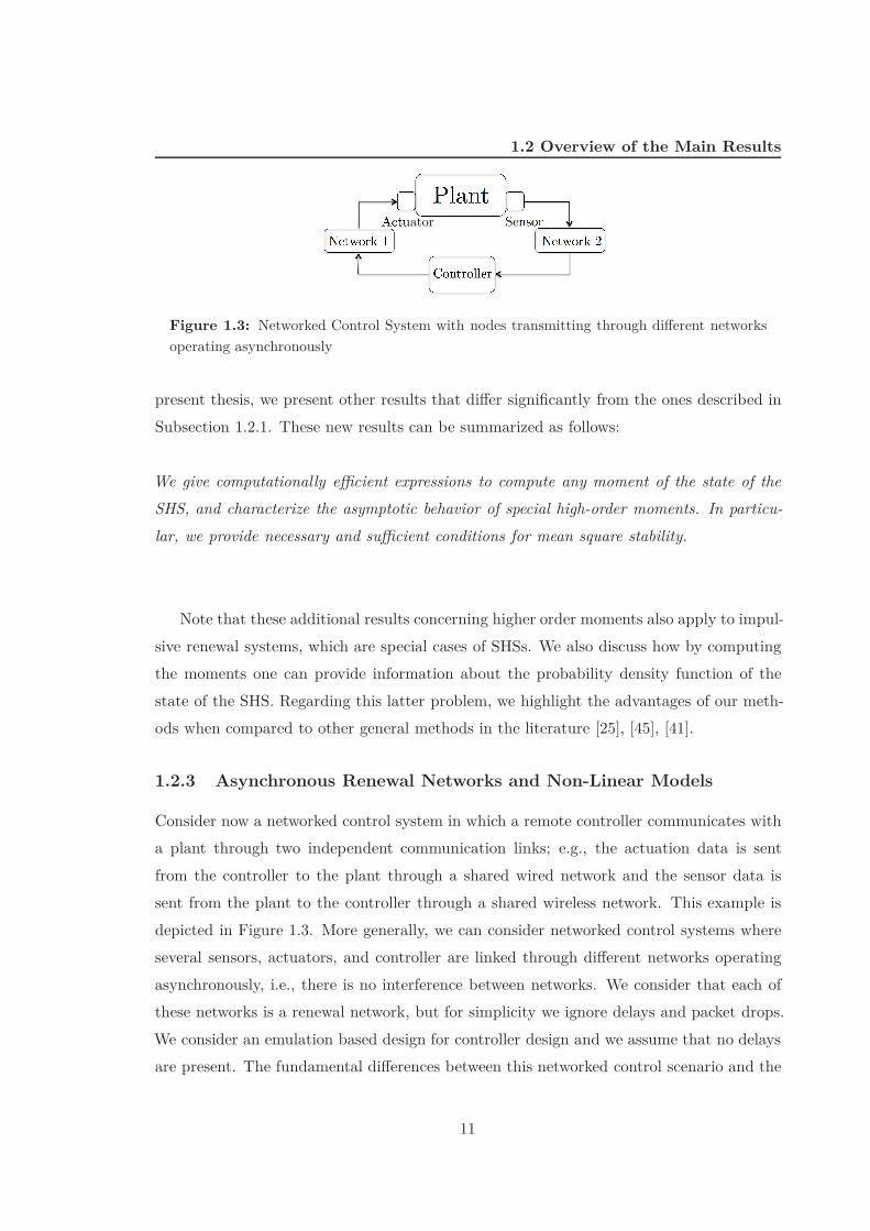
1.1 General Diagram of a Networked Control System . . . . . . . . . . . . . . . 41.2 Two possible scenarios where a single node transmits through a shared network 81.3 Networked Control System with nodes transmitting through di!erent net-
works operating asynchronously . . . . . . . . . . . . . . . . . . . . . . . . . 111.4 Multi-Rate networked control systems setup . . . . . . . . . . . . . . . . . . 15
2.1 Nyquist plot illustration of stability for the impulsive renewal pendulumsystem. . . . . . . . . . . . . . . . . . . . . . . . . . . . . . . . . . . . . . . 29
2.2 MIMO LTI closed loop . . . . . . . . . . . . . . . . . . . . . . . . . . . . . . 43
3.1 Plot of E[e(t)], where e(t) is quadratically state dependent. For a fixed t,E[e(t)] lies between the dashed curves with probability > 3
4 . . . . . . . . . . 69
4.1 MES for various values of the support of a uniform distributions of thetransmission intervals of two independent links. . . . . . . . . . . . . . . . . 85
6.1 Proposed controller structure to achieve output regulation; Plant:P; Con-troller: CI -internal model, CD blocking system, CK stabilizer . . . . . . . . 131
6.2 yr[k] and r[k]. . . . . . . . . . . . . . . . . . . . . . . . . . . . . . . . . . . . 1386.3 Various closed-loop signals . . . . . . . . . . . . . . . . . . . . . . . . . . . . 139
7.1 Regulator structure for non-square systems . . . . . . . . . . . . . . . . . . 1637.2 Gain-scheduled and linear controller . . . . . . . . . . . . . . . . . . . . . . 1697.3 Actuation and multi-rate inputs ym1 and ym2 . . . . . . . . . . . . . . . . . 1697.4 Slow and fast ramp response . . . . . . . . . . . . . . . . . . . . . . . . . . 1707.5 Block diagram with the final implementation scheme . . . . . . . . . . . . . 1757.6 Results for the first simulation- Errors . . . . . . . . . . . . . . . . . . . . . 1777.7 Results for the first simulation- Actuation . . . . . . . . . . . . . . . . . . . 178
ix

LIST OF FIGURES
7.8 Results for the second simulation . . . . . . . . . . . . . . . . . . . . . . . . 1797.9 Rotorcraft Maneuvers . . . . . . . . . . . . . . . . . . . . . . . . . . . . . . 180
x
List of Tables
2.1 Variation of the Lyapunov exponent of (2.16) with the support ! of for theinter-sampling distribution . . . . . . . . . . . . . . . . . . . . . . . . . . . . 30
3.1 Stability conditions for the Batch Reactor Example . . . . . . . . . . . . . . 673.2 Exponential decay rates E[e(t)] ! ce!!t . . . . . . . . . . . . . . . . . . . . 68
5.1 Stability results for the batch reactor example-MEF-TOD and Round Robinprotocol. NA stands for Not Available . . . . . . . . . . . . . . . . . . . . . 113
5.2 Stability results for the batch reactor example-Protocol design, no packetdrops . . . . . . . . . . . . . . . . . . . . . . . . . . . . . . . . . . . . . . . . 114
5.3 Performance of base (periodic) and rollout policies for the pendulum example121
7.1 H2 closed-loop values for di!erent position sampling rates . . . . . . . . . . 176
xi

LIST OF TABLES
xii

1
Introduction
In recent years we have witnessed remarkable technological advances in computing, sens-ing and wireless communication technologies. The combination of these advances madepossible pocket-size embedded electronic devices, designed to sense, compute, and commu-nicate information of interest. Sensors and micro-processors are now ubiquitously deployedin vehicles, roads, cell-phones, buildings, and environment, and have the ability to processmeasurement data in real time and transmit this data to perform adequate control actions.A control system where sensors, micro-controllers, and actuators are connected throughcommunication networks is termed a Networked Control System (NCS).
There are abundant new and envisioned applications of networked control systems [43].As a first example, consider the problem of preventing highways’ tra"c congestions. A re-quirement for providing tra"c control is to predict tra"c conditions. This can be achievedby using a limited number of vehicle detector stations (sensors) deployed along the highway.A networked control estimation problem is to infer on the highway tra"c density from thesedistributed measurements [37], [70]. Another research direction is the control of vehicleplatoons [30] to mitigate the so-called butterfly e!ect, i.e., large tra"c jams triggered byminor events, such as an abrupt steering maneuver by a single motorist. Here, the goalis to control the velocities and relative positions of the vehicles based on communicationfrom immediate predecessors, so that a desired behavior for the platoon is achieved, e.g.,constant speed cruising or leader following. As a second class of applications, consider theemerging field of smart grids. It is predicted that in a near future renewable energy sources,such as wind and solar power, will play an even more important role in the overall energyproduction. However, the uncertainty on the availability of such energy sources, along withthe increasingly variability of loads, such as electric vehicles, poses challenging problems
1
1. INTRODUCTION
concerning the transient stability of the network, i.e., achieving synchronism when sub-jected to these large disturbances on load and generation. In [29], the relation between thetransient analysis in a power network and a distributed networked control problem knownas the consensus problem is sharply recognized. Another example in the area of energysystems is the use of sensor networks in energy building e"ciency, which enables improvedcontrol of indoor environment [92]. As a third class of applications, consider automationin manufacturing systems. Here, communication networks are being used more and morefor diagnostic and control operations [71]. The use of wireless communications in industryenvironments can drastically reduce cabling and maintenance costs. However, the mea-surement and control delays resulting from introducing a shared communication mediumhave to be taken into account when designing such systems. There are several other appli-cations in many distinct fields, such as remote surgery [67], or thermal control of livestockstables [96]. Also in a luxury car there may exist over 50 embedded computers, runningseveral control algorithms, which include safety critical operations, as well as leisure appli-cations [83]. Using a network to close the control loop has several advantages, includingflexibility, high reliability, simple installation and maintenance, and low cost. The demandfor small and intelligent sensing devices is steadily growing in our society, which allowsone to predict that networked control systems will continue to be a prominent object ofinterest in coming years.
On the other hand, the interest on networked control system is far from confiningitself to the realm of applications. Networked control systems have given rise to a multi-disciplinary research field lying in the intersection of three distinct research areas: con-trol systems, telecommunications, and computer science, and this has promoted the inter-change of problem solving techniques and insights from di!erent areas. Moreover, someof the problems that arise in networked control lead to important research advances inthe control research field. For example, the celebrated Shannon’s results on the maximumbit-rate at which a communication channel can carry information reliably, has inspiredseveral researchers [31, 42, 72, 94], to tackle the problem of determining the minimumbit-rate needed to stabilize a linear system through feedback over a finite capacity chan-nel. Stochastic and deterministic hybrid systems [45], [77], have played an important rolein modeling several networked control scenarios, and several theoretical results promptedfrom this relation [62], [90], [73]. The inherent distributed structure of many problemsin networked control system has also inspired many problems in the area of distributedcontrol of agents deployed in a given environment [12]. There are several problems where
2

agents are connected by a communication network and wish to optimize a given perfor-mance cost in a distributed way [49] or achieve a common objective [10]. Hence, there is asignificant overlap between the research on networked control systems and the research ondistributed optimization and decentralized control. Another example are switched systems,where recognizing the connection with networked control system has favored research onboth areas [28], [36].
In this thesis, we formulate and address several networked control problems, consideringthree models for the communication network: (i) networks with stochastic characteristics,where the arbitration process for network access involves stochastic events, such as ran-dom delays, packet drops, or random back-o! times. Examples of networks where suchevents may occur are the Ethernet and networks utilizing the Wireless 802.11 protocol;(ii) networks in which access to the network is determined by a protocol based on stateinformation sent by the nodes. This may be achieved in networks where nodes have enoughcomputational resources to run an arbitration algorithm in a distributed way, or in caseswhere the network itself may provide an arbitration mechanism based on data sent by thenodes, e.g., CAN-BUS networks. Since decisions are dynamically taken at each transmis-sion time based on state information, we denote these protocols by dynamic protocols; (iii)networks with periodic multi-rate data transmissions, where each communication link hasa fixed rate, which is in general di!erent from the rates of the other links. Examples ofthese networks are the circuit switching networks, which guarantee a fixed bandwidth foreach link.
The solutions we propose often involve developing novel theoretical and system analyti-cal results. In fact, it is a common trend in the thesis that the underlying networked controlproblem serves as a motivation or as a starting point to consider mathematical and systemanalytical problems obtained from raising the level of abstraction of the models that cap-ture the networked control problem. As we shall see, this approach has the advantage thatour results often have a broader range of application that exceeds the networked controlsystems scope. We use the framework of hybrid systems to model the networked controlsystems that we consider and the machinery of Volterra equations, piecewise deterministicprocesses, and dynamic programming to establish the main results of the thesis.
In this introductory chapter, we give a general description of the networked controlproblems that we tackle in Section 1.1 and provide an overview of our main results in Sec-tion 1.2. We explain the organization of the thesis in Section 1.3 and enumerate the thesis
3
1. INTRODUCTION
Figure 1.1: General Diagram of a Networked Control System
contributions, as well as the list of publications that substantiate the thesis in Section 1.4.Basic notation is established in Section 1.5.
1.1 Networked Control Systems - General Description
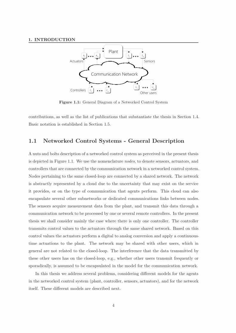
A nuts and bolts description of a networked control system as perceived in the present thesisis depicted in Figure 1.1. We use the nomenclature nodes, to denote sensors, actuators, andcontrollers that are connected by the communication network in a networked control system.Nodes pertaining to the same closed-loop are connected by a shared network. The networkis abstractly represented by a cloud due to the uncertainty that may exist on the serviceit provides, or on the type of communication that agents perform. This cloud can alsoencapsulate several other subnetworks or dedicated communications links between nodes.The sensors acquire measurement data from the plant, and transmit this data through acommunication network to be processed by one or several remote controllers. In the presentthesis we shall consider mainly the case where there is only one controller. The controllertransmits control values to the actuators through the same shared network. Based on thiscontrol values the actuators perform a digital to analog conversion and apply a continuous-time actuations to the plant. The network may be shared with other users, which ingeneral are not related to the closed-loop. The interference that the data transmitted bythese other users has on the closed-loop, e.g., whether other users transmit frequently orsporadically, is assumed to be encapsulated in the model for the communication network.
In this thesis we address several problems, considering di!erent models for the agentsin the networked control system (plant, controller, sensors, actuators), and for the networkitself. These di!erent models are described next.
4

1.1 Networked Control Systems - General Description
Plant
The model for the plant may be linear or nonlinear, certain or uncertain. Uncertaintymay be modeled by external stochastic disturbances, or by external deterministic (butunknown) disturbances. It may also be the case that there exists parameter uncertainty onthe plant.
Controller Synthesis
Tracing a parallel with traditional digital control [15], we consider two methods for obtain-ing the controller: emulation and direct design. In emulation, a continuous-time stabilizingcontroller designed without regard to the network characteristics is assumed to be avail-able. The controller for the networked control system is obtained by running a numericalapproximation method of the continuous-time controller based on the measurement valuesreceived from the sensors. This numerical approximation is typically obtained by emu-lating the evolution of the continuous-time controller using as its inputs hold values ofthe measurement data most recently received from the sensors. Both sensor measurementarrivals and transmissions of actuation updates from the controller to the actuators aredictated by the communication networks availability. From a networked control point ofview, for an emulation design, we are simply concerned with analyzing the e!ects of thenetwork in the closed-loop. On the other hand, in direct design the controller for the net-worked control system is synthesized by directly taking into account the plant and networkcharacteristics. The specifications to obtain this controller can be closed-loop stability, op-timality according to some performance criterion, and/or output regulation of some outputsof interest.
Sensors and actuators
Sensors perform an analog to digital conversion, which is assumed to be an ideal sampling,while actuators perform a digital to analog conversion which is typically assumed to bea standard hold operation, although other possibilities exist (cf. [69], [63]). Sensors andactuators are assumed to have network adapters to transmit data through the network.Each sensor may be associated with more than one output of the plant’s state, and eachactuator may be associated with more than one input of the plant. In cases where sensorsand actuators have dedicated links to transmit, we may only need to assume that theycan be sampled and updated (respectively) at a fixed rate, while in general we shall re-quire that they can be sampled and updated on demand, i.e., at any desired transmission
5
1. INTRODUCTION
time. We denote sensors and actuators by simple sensors and simple actuators if thesesampling and transmitting operations are the only operations they can perform. However,we denote sensors by smart sensors if they have enough computational resources to runan arbitration algorithm for network access, and denote controllers by smart controllers ifthey are collocated with the actuators, in which case we also assume that they have enoughcomputational resources to run an arbitration algorithm.
Network
The network access in a shared network typically introduces delays, since nodes may haveto wait until the network becomes available. Depending on the implementation or con-text, these delays may either a!ect the times between consecutive sampling, in cases wheresensors and controllers respond on demand to network availability, or may introduce sig-nificant delays on the data received from plant and controller, in case the sensors holdpast information until the network becomes available for transmission. Further delays maybe taken into account such as transmission and processing delays. In this thesis, we shallmainly consider the following model for a network with stochastic characteristics, whichwe denote by renewal network, a nomenclature justified in the sequel.
(i) The time intervals between transmissions from nodes pertaining to the networkedcontrol system are independent and identically distributed;
(ii) The transmission delays are small when compared to the time intervals betweentransmissions;
(iii) Packet may me dropped with a given probability.
Assumption (i) holds for scenarios in which nodes attempt to do periodic transmissionsof data, but these regular transmissions may be perturbed by the medium access proto-col. It is typically the case in CSMA protocols that nodes may be forced to back-o! fora typically random amount of time until the network becomes available. The probabilitydistribution of the time interval between transmissions, which can be estimated experimen-tally or by running Monte Carlo simulations of the protocol, is determined by two factors:the congestion of the network and the delay introduced by the medium access protocol.Assumption (ii) also holds in general in local area networks. In fact, as explained in [90],in local area networks, the transmission delays are typically small when compared to thetimes that nodes take to gain access to the communication medium. We shall considergeneral stochastic models for the delays (see Chapter 3, Sec. 3.1, and Chapter 5, Sec 5.1.1).
6
1.2 Overview of the Main Results
Assumption (iii) is typical and our modeling framework allows to consider general modelswhere packet drop are correlated and modeled by Markov Chains (see Chapter 3) such asthe well-known Gilbert-Elliot model. We use the nomenclature renewal network, since thestate variables associated with the sources of randomness (intervals between transmissions,delays, packet drops) restart or are renewed when a transmission occurs.
Another model that will be used in the present thesis is to assume that each sensor andeach actuator use a di!erent communication link to exchange data with the controller. Eachcommunication link may represent a shared network that guarantees a fixed transmissionrate, such as in circuit switching networks (cf. [58]). It can also simply represent a sensor,which outputs measurements at a fixed sampling rate, or an actuator which allows actuationupdates at a fixed rate. We denote these networks by multi-rate networks.
Access Protocol
Typical communication networks, such as the wireless 802.11, the Ethernet, and the CAN-BUS, provide a medium access protocol for transmissions. However, what we mean hereby access protocol is the high-level protocol that nodes pertaining to the same loop maypossibly implement on top of the protocol provided by the network. A static protocol isdefined as a protocol in which the nodes agree to transmit in a prescribed order, which isrepeated periodically. Note that in a static protocol a node is allowed to transmit more thanonce in a period. On the other hand, one can define dynamic protocols, running on-line,i.e., simultaneously with the process, in which nodes are allowed to arbitrate who transmitsbased on state information about the plant and/or based on the data received from previoustransmissions. Dynamic protocols may utilize some mechanism for arbitration provided bysome networks, e.g., dynamically changing the arbitration field of messages in CAN-BUSnetworks. However, in general, nodes run an arbitration algorithm in a distributed wayand on top of an underlying communication protocol which o!ers no direct service forarbitration, in which case we assume that the sensors and actuator nodes are smart.
1.2 Overview of the Main Results
We divide the presentation of our main results according to six works that substantiate thethesis. The first three works focus on analytical properties of networked control systemsin which the network has stochastic characteristics. The fourth work proposes a classof dynamic protocols for networked control systems, and the fifth and sixth works studynetworked control systems with periodic multi-rate transmissions. In each of these works we
7
1. INTRODUCTION��
Plant Controller
Actuator Sensor
Network
(a) Controller collocated with sensor
���������������
PlantController
Actuator Sensor
Network
(b) Controller collocated with actuator
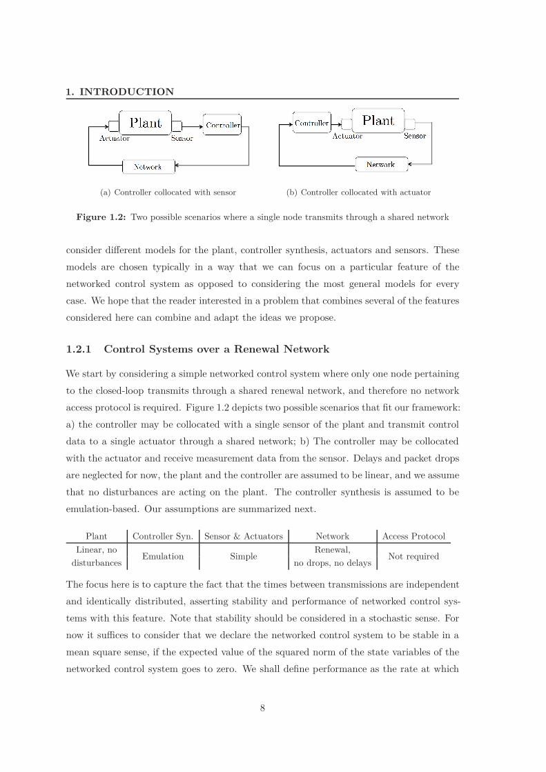
Figure 1.2: Two possible scenarios where a single node transmits through a shared network
consider di!erent models for the plant, controller synthesis, actuators and sensors. Thesemodels are chosen typically in a way that we can focus on a particular feature of thenetworked control system as opposed to considering the most general models for everycase. We hope that the reader interested in a problem that combines several of the featuresconsidered here can combine and adapt the ideas we propose.
1.2.1 Control Systems over a Renewal Network
We start by considering a simple networked control system where only one node pertainingto the closed-loop transmits through a shared renewal network, and therefore no networkaccess protocol is required. Figure 1.2 depicts two possible scenarios that fit our framework:a) the controller may be collocated with a single sensor of the plant and transmit controldata to a single actuator through a shared network; b) The controller may be collocatedwith the actuator and receive measurement data from the sensor. Delays and packet dropsare neglected for now, the plant and the controller are assumed to be linear, and we assumethat no disturbances are acting on the plant. The controller synthesis is assumed to beemulation-based. Our assumptions are summarized next.
Plant Controller Syn. Sensor & Actuators Network Access ProtocolLinear, no Emulation Simple Renewal, Not requireddisturbances no drops, no delays
The focus here is to capture the fact that the times between transmissions are independentand identically distributed, asserting stability and performance of networked control sys-tems with this feature. Note that stability should be considered in a stochastic sense. Fornow it su"ces to consider that we declare the networked control system to be stable in amean square sense, if the expected value of the squared norm of the state variables of thenetworked control system goes to zero. We shall define performance as the rate at which
8

1.2 Overview of the Main Results
the expected value of a quadratic positive definite function of the state goes to zero.
We show that the networked control system just described can be modeled by animpulsive renewal system. Impulsive renewal systems are described by a vector field thatdetermines the evolution of the state between transition times at which the state undergoesa jump determined by a reset map. The intervals between transition times are assumedto be independent and identically distributed (i.i.d.) random variables. The nomenclatureimpulsive renewal system is motivated by the fact that the process that counts the numberof transitions up to the current time is a renewal process (cf. [79]). We provide analyticalresults for impulsive renewal systems, which are deeply rooted in a set of novel results forVolterra integral equations with positive kernel, and have applications to the stability anal-ysis of the networked control systems depicted in Figure 1.2. Volterra integral equationswith positive kernel shall be defined in Chapter 2, where we also provide general results forthis class of equations and show other applications of these results. The main implicationsof these results for networked control systems can be summarized as follows.
We provide stability conditions for impulsive renewal systems that can be cast in termsof a matrix eigenvalue computation, the feasibility of a set of LMIs, and also tested usingthe Nyquist criterion. Moreover, we provide a method to compute a second moment Lya-punov exponent, which provides the asymptotic rate of decrease / growth for the expectedvalue of a quadratic function of the systems’ state. These results have a direct applicationto NCSs with a single renewal network.
We also discuss how one can assert the performance of the networked control system withsingle renewal network by computing the second moment Lyapunov exponent of the im-pulsive renewal system.
Our framework shares common features with randomly sampled systems [40], [55]. Aswe shall discuss in Chapter 2, our results, to the best of our knowledge, have not beenobtained before, and shed further insight also to randomly sampled systems.
We consider the problem of directly designing a controller in this framework in [AHS09a].However, since the results one obtains using a dynamic programming optimal control frame-work are similar to existing results for randomly sampled systems [40], [55], we decide not toinclude them in the present thesis. The interested reader can consult [AHS09a], [40], [55].
9

1. INTRODUCTION
1.2.2 Network Features Modeled by Finite State Machines
Consider now that several nodes pertaining to the same closed-loop are connected to thenetwork, implementing a static protocol, and also the general case where the network mayhave delays and packet drops. The remaining assumptions on the networked control systemare similar to the ones considered in Section 1.2.1 and are summarized next.
Plant Controller Syn. Sensor & Actuators Network Access ProtocolLinear, no Emulation Simple Renewal, Staticdisturbances with drops & delays
We will show that static protocols, delays, packet drops, and other network features whichcan be captured by finite state machines can be modeled by stochastic hybrid systems.
Stochastic hybrid systems (SHSs) are systems with both continuous dynamics anddiscrete logic. The execution of an SHS is specified by the dynamic equations of thecontinuous state, a set of rules governing the transitions between discrete modes, and resetmaps determining jumps of the state at transition times. We consider SHSs with lineardynamics, linear reset maps, and for which the lengths of times that the system stays ineach mode are independent arbitrarily distributed random variables, whose distributionsmay depend on the discrete mode. The process that combines the transition times andthe discrete mode is called a Markov renewal process [48], which motivated us to refer tothese systems as stochastic hybrid systems with renewal transitions. The class of impulsiverenewal systems is a special case of a SHS with renewal transitions, where there is only onediscrete mode and only one reset map. The key to model networked control system withSHSs is to capture the sequence of events as a finite state machine. As we will show inChapter 3, besides delays, packet drops, and static protocols we can capture, e.g., scenarioswhere nodes try to access the network independently, or scenarios where nodes transmitthrough more than one renewal network, operating synchronously.
Inspired by the work on impulsive renewal systems, the approach followed to analyzestochastic hybrid systems with renewal transitions is based on a set of Volterra renewal-typeequations. As for impulsive renewal systems, we can characterize the asymptotic behaviorof the system by providing necessary and su"cient conditions for various stability notionsin terms of LMIs, algebraic expressions and Nyquist criterion conditions, and determiningthe decay or increase rate at which the expected value of a quadratic function of the sys-tems’ state converges exponentially fast to zero or to infinity, depending on whether or notthe system is mean exponentially stable. We derived these results in [AHS10b]. In the
10
1.2 Overview of the Main Results
Plant
Controller
Actuator Sensor
Network 1 Network 2
Figure 1.3: Networked Control System with nodes transmitting through di!erent networksoperating asynchronously
present thesis, we present other results that di!er significantly from the ones described inSubsection 1.2.1. These new results can be summarized as follows:
We give computationally e!cient expressions to compute any moment of the state of theSHS, and characterize the asymptotic behavior of special high-order moments. In particu-lar, we provide necessary and su!cient conditions for mean square stability.
Note that these additional results concerning higher order moments also apply to impul-sive renewal systems, which are special cases of SHSs. We also discuss how by computingthe moments one can provide information about the probability density function of thestate of the SHS. Regarding this latter problem, we highlight the advantages of our meth-ods when compared to other general methods in the literature [25], [45], [41].
1.2.3 Asynchronous Renewal Networks and Non-Linear Models
Consider now a networked control system in which a remote controller communicates witha plant through two independent communication links; e.g., the actuation data is sentfrom the controller to the plant through a shared wired network and the sensor data issent from the plant to the controller through a shared wireless network. This example isdepicted in Figure 1.3. More generally, we can consider networked control systems whereseveral sensors, actuators, and controller are linked through di!erent networks operatingasynchronously, i.e., there is no interference between networks. We consider that each ofthese networks is a renewal network, but for simplicity we ignore delays and packet drops.We consider an emulation based design for controller design and we assume that no delaysare present. The fundamental di!erences between this networked control scenario and the
11
1. INTRODUCTION
one considered in the previous subsections are two fold: (i) the networks operate asyn-chronously, (ii) the model for the plant and for the controller are allowed to be non-linear.We still consider no disturbances in the model for the plant, and we assume for simplicitythat no two nodes transmit through the same shared network. Our assumptions are sum-marized next.
Plant Controller Syn. S & A Network Access ProtocolLinear & non-linear Emulation Simple Asynchronous Renewal Not requiredno disturbances links, no drops, no delays
We could model several renewal networks in the networked control system with the frame-work of stochastic hybrid systems, as long as the protocols could be modeled as finite statemachines. However, since each renewal network operates asynchronously, it does not ap-pear to be possible to capture this scenario with finite state machines. This significantlychanges the type of mathematical tools used to address these systems and the correspond-ing results. In fact, the approach we follow for the networked control scenarios consideredin Sections 1.2.1 and 1.2.2, based on Volterra integral equations, does not appear to renderan easy extension to the present case of asynchronous networks. Piecewise deterministicprocesses [25] are shown to be an adequate mathematical framework to tackle these sys-tems. Interestingly, they also allow to handle the case of non-linear models for the plantand the controller.
We show that the networked control system at hand can be modeled by an impulsivesystem triggered by a superposed renewal process, which is a model similar to impulsiverenewal systems but allowing several reset maps triggered by independent renewal pro-cesses, i.e., the intervals between jumps associated with a given reset map are identicallydistributed and independent of the other jump intervals. The connection between this classof systems and piecewise deterministic processes is also addressed. We provide stabilityresults for this new class of impulsive systems, which directly entail stability properties forthe considered asynchronous networked control systems. Our main results can be summa-rized as follows.
We provide stability conditions for general non-linear NCSs with asynchronous links. Byspecializing these stability conditions to linear NCSs, we show that stability for linear NCSscan be asserted by testing if the spectral radius of an integral operator is less than one.
12
1.2 Overview of the Main Results
We also show that the origin of the non-linear NCS is stable with probability oneif its linearization about zero equilibrium is mean exponentially stable, which justifiesthe importance of studying the linear case. Stability with probability one is a standardgeneralization of the notion of local stability to stochastic systems, and will be formallydefined in Chapter 4.
1.2.4 Dynamic Protocols
We have already discussed time-driven static protocols in which nodes choose a given orderto transmit, which is repeated periodically. However, it is reasonable to suspect that insome state configurations of the networked control system it may be more favorable forone of the nodes to transmit, whereas for other states, transmissions from other nodes maylead to more favorable outcomes. This leads us to study dynamic protocols, in which nodesare allowed to arbitrate who transmits based on state information about the plant and/orbased on the data received from previous transmissions. We tackle this problem from boththe frameworks of emulation and direct design for controller synthesis. The plant is con-sidered to be linear, and in the controller design setup we shall consider a model where theplant is disturbed by Gaussian noise. The sensors and actuators are assumed to be smart,i.e., to have enough computation resources to run an arbitration algorithm, and we alsoconsider delays and packet drops. Our assumptions are summarized next.
Plant Controller Syn. S & A Network Access ProtocolLinear, with and Emulation & Smart Renewal, Dynamicwithout disturbances direct design with drops and delays
Considering an emulation framework, we provide conditions for mean exponential sta-bility of the networked closed-loop in terms of matrix inequalities, both for investigatingthe stability of given protocols, such as static round-robin protocols and dynamic maximumerror first-try once discard protocols [91], and to design new dynamic protocols. The mainresult entailed by these conditions is that if the networked closed-loop is stable for a staticprotocol, then we can provide a dynamic protocol for which the networked closed-loop isalso stable. The dynamic protocol in this case can be obtained by construction. However,the obtained protocol assumes in general that the full-state is available, which restricts therange of applicability of the results in this emulation framework.
Considering a direct design framework, we tackle the problem of simultaneously de-signing the scheduling sequence of transmissions and the control law, so as to optimize a
13
1. INTRODUCTION
quadratic objective. The plant is assumed to be disturbed by noise. Using the frameworkof dynamic programming, we propose a rollout strategy [5] by which the scheduling andcontrol decisions are determined at each transmission time as the ones that lead to optimalperformance over a given horizon, assuming that from then on controller and sensors trans-mit in a periodic order and the control law is a standard optimal law for periodic systems.We show that this rollout strategy results in a protocol where scheduling decisions arebased on the state estimate and error covariance matrix of a Kalman estimator, and mustbe determined on-line (closed-loop policy) in the case where both control and measurementvalues are scheduled. This is in striking contrast with the optimal and analog rollout strate-gies for the sensor scheduling problem [68], in which only the sensors are to be schedulingwhile the control variables can be updated at every time step (e.g., controller is collocatedwith the plant), for which the scheduling sequence can be determined o!-line (open looppolicy). The resulting protocol obtained from the rollout algorithm can be implemented ina distributed way both in wireless and wired networks, based on previous data sent fromsensors and actuators, as opposed to the requirements of the protocol obtained with theemulation framework, where full-state is in general required. It follows by constructionof rollout algorithms that our proposed scheduling method can outperform any periodicscheduling of transmissions. Our main results both for emulation and direct design can besummarized as follows.
We propose a class of dynamic protocols for both the cases of emulation and direct de-sign that result directly from stability and optimal solutions to the problem at hand. Theprotocol for an emulation design depends on state information of the networked controlsystem, whereas the protocol obtained in the direct design framework depends on state es-timates of the plant and can be run in a distributed way. In both frameworks, dynamicprotocols are shown to outperform periodic protocols.
1.2.5 Output Regulation for Multi-Rate Systems
The output regulation problem consists on controlling the output of a linear time-invariantplant so as to achieve asymptotic tracking of an exogenous signal generated by the freemotion of a linear time-invariant system, so-called exosystem, while guaranteeing closed-loop stability. Here we tackle the output regulation problem when sensors transmit overdi!erent dedicated links imposing di!erent transmission rates. We consider linear plants
14
1.2 Overview of the Main Results
Figure 1.4: Multi-Rate networked control systems setup
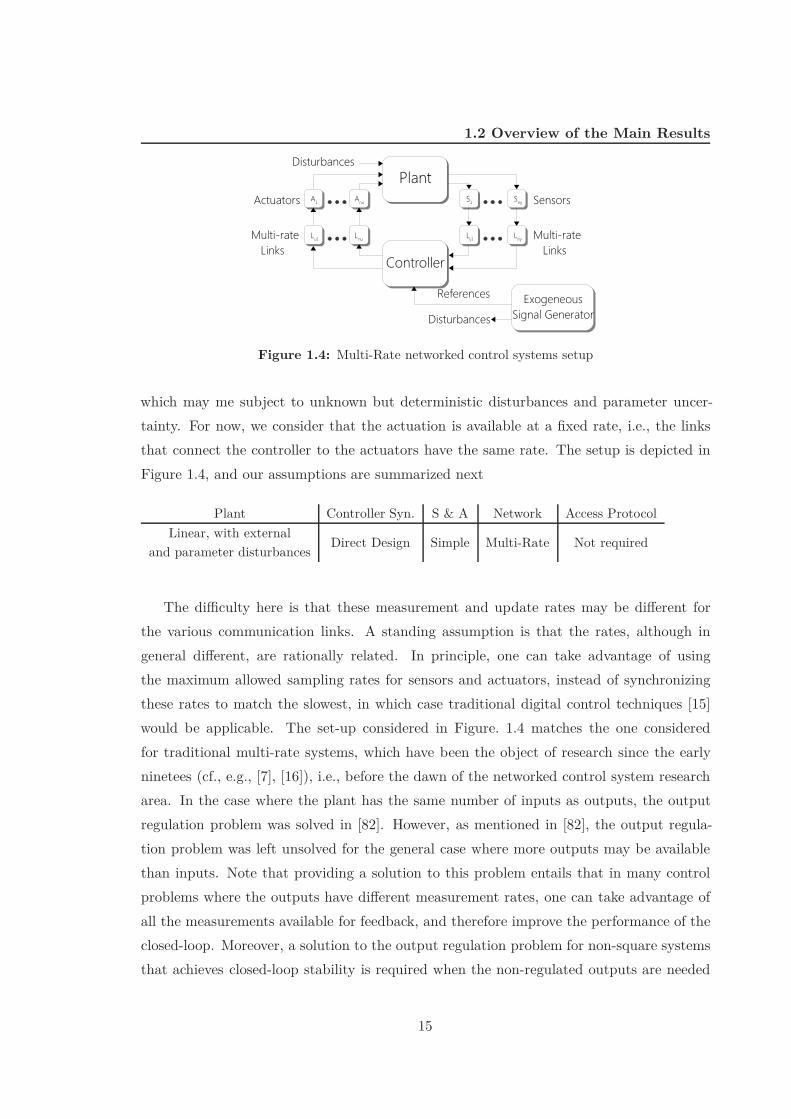
which may me subject to unknown but deterministic disturbances and parameter uncer-tainty. For now, we consider that the actuation is available at a fixed rate, i.e., the linksthat connect the controller to the actuators have the same rate. The setup is depicted inFigure 1.4, and our assumptions are summarized next
Plant Controller Syn. S & A Network Access ProtocolLinear, with external Direct Design Simple Multi-Rate Not requiredand parameter disturbances
The di"culty here is that these measurement and update rates may be di!erent forthe various communication links. A standing assumption is that the rates, although ingeneral di!erent, are rationally related. In principle, one can take advantage of usingthe maximum allowed sampling rates for sensors and actuators, instead of synchronizingthese rates to match the slowest, in which case traditional digital control techniques [15]would be applicable. The set-up considered in Figure. 1.4 matches the one consideredfor traditional multi-rate systems, which have been the object of research since the earlyninetees (cf., e.g., [7], [16]), i.e., before the dawn of the networked control system researcharea. In the case where the plant has the same number of inputs as outputs, the outputregulation problem was solved in [82]. However, as mentioned in [82], the output regula-tion problem was left unsolved for the general case where more outputs may be availablethan inputs. Note that providing a solution to this problem entails that in many controlproblems where the outputs have di!erent measurement rates, one can take advantage ofall the measurements available for feedback, and therefore improve the performance of theclosed-loop. Moreover, a solution to the output regulation problem for non-square systemsthat achieves closed-loop stability is required when the non-regulated outputs are needed
15
1. INTRODUCTION
to guarantee the detectability of the plant. In this thesis we present the following result.
We design a controller that achieves stability for the closed-loop and output regulation fora number of regulated outputs equal to the number of inputs, while taking advantage of theremaining outputs for feedback.
1.2.6 Gain-scheduling Control for Multi-Rate Systems
Gain-scheduling is a useful tool for designing control laws for non-linear plants, using linearcontrol tools [53]. The standard procedure for designing a gain-scheduling controller in-volves the following steps (cf. [81]): (i) the selection of scheduling variables or parameters;(ii) linearization of the non-linear plant about the equilibrium manifold; (iii) synthesis ofcontrollers for the family of plant linearizations, which typically involves linear controllerdesign for a given set of equilibrium points; and (iv) implementation of the controller. Theimplementation must be such that the controller verifies the linearization property: at eachequilibrium point, the nonlinear gain-scheduled controller must linearize to the linear con-troller designed for that equilibrium. In fact, it is often the case that for gain-schedulingimplementations which would perhaps appear more natural the linearization property doesnot hold and this mismatch is commonly known as the hidden coupling [81]. A solutionto part (iv) is the velocity implementation proposed in [52] and further discussed in [53,Ch. 12], [81]. In the present thesis, we pose the problem of obtaining a solution to thegain-scheduling problem in the case where actuators and sensors have di!erent rates. Theplant is assumed to be non-linear and subject to external deterministic but unknown dis-turbances and we assume that the model for the plant may have parameter uncertainty.Our assumptions are summarized next
Plant Controller Syn. S & A Network Access ProtocolNon-Linear, with external Direct Design Simple Multi-Rate Not requiredand parameter disturbances
In this thesis we have the following results.
We provide a method for the synthesis and implementation of gain-scheduled controllersfor multi-rate systems that satisfies the linearization property, and show that the proposedimplementation satisfies similar stability properties to the ones considered for linear time
16

1.3 Organization of the Thesis
invariant systems [53].
Gain-scheduling control is a tool per excellence in guidance, navigation and control prob-lems. As an application, we cast the integrated guidance and control problem for anautonomous vehicles as a regulation problem, and using our results we are able to solve ina systematic manner the guidance and control problem for autonomous vehicles equippedwith multi-rate sensor suite. The methodology is applied to the trajectory tracking problemof steering an autonomous rotorcraft along a pre-defined trajectory.
1.3 Organization of the Thesis
The organization of the thesis is dictated by the mentioned six networked control problemsthat we tackle. We devote a chapter to each. Networked control systems with a singlenode transmitting though a renewal network are addressed in Chapter 2, networked controlsystems modeled by finite state machines are addressed in Chapter 3, and networked controlsystems with asynchronous networks are addressed in Chapter 4. Chapter 5 is devotedto dynamic protocols, while Chapters 6 and 7 address the output regulation and gain-scheduling problems for multi-rate systems, respectively. Final conclusions and remarks,as well as future work are provided in Chapter 8.
1.4 Contributions and List of Publications
The publications that substantiate the present thesis are listed after the bibliography. Wesummarize next the already described contributions for stochastic, dynamic, and periodicnetworked control systems, and the corresponding publications where these contributionscan be found.
• Stability conditions and determination of Lyapunov exponents for NCSs with a singlerenewal network [AHS11d], [AHS09b], [AHS09a].
• Transitory and asymptotic moment analysis for NCSs with network features modeledby finite state machines [AHS11b], [AHS10b].
• Stability conditions for NCSs with asynchronous renewal networks [AHS10a],[AHS11a].
• Propose a class of dynamic protocols that always outperform static ones [AHS11],[AHS11c], [AHHS11a], [AHHS11b].
17
1. INTRODUCTION
• A solution to the output regulation problem for multi-rate systems [ASH11].
• A solution to the gain-scheduling problem for multi-rate systems [ASC07], [ASC08a],[ASC08b], [ASC10].
In the process of solving these networked control problems we found other results whichare important per se. These results are listed next, where we also provide the articles andthe section of the thesis where they can be found. More details on these results are giventherein.
• Definition and stability analysis of Volterra Equations with Positive Kernel [AHS11d],Section 2.7.
• Stability results for piecewise deterministic processes [AHS10a], Section 4.3.1.
• Definition of blocking zero with respect to a matrix both for linear time-invariantsystems and for periodically time-varying systems [ASH11], Section 6.4.
1.5 Basic Notation and Nomenclature
For a given matrix A, its transpose is denoted by A!, its hermitian by A", its trace bytr(A), its spectral radius by r"(A), and an eigenvalue by "i(A). We use A > 0 (A " 0) todenote that a real or complex symmetric matrix is positive definite (semi-definite). Then#n identity and zero matrices are denoted by In and 0n, respectively, and the notation 1n
indicates a vector of n ones. The dimensional information is dropped whenever no confusionarises. For dimensionally compatible matrices A and B, we define (A, B) := [A! B!]!.We denote by diag([A1 . . . An]) a block diagonal matrix with blocks Ai. The Kroneckerproduct is denoted by $. The expected value is denoted by E(.). For a complex numberz, %[z] and &[z] denote the real and complex parts of z, respectively. The notation x(t!
k )indicates the limit from the left of a function x(t) at the point tk. When we work infinite dimensional spaces, these are identified with Cn, or Rn, subsumed to be Hilbertspaces with the usual inner product 'x, y( = y"x, Banach spaces with the usual norm)x)2 = 'x, x( and endowed with the usual topology inherited by the norm. We considerthe usual vector identifications Cn#n *= Cn2, Rn#n *= Rn2 for matrices and this results inthe following inner product 'A, B( = tr(B"A). We denote the value at time t + R$0 ofthe continuous-time signals x : R$0 ,- Rn by x(t), and the value at time k + N of thediscrete time signals x : N ,- Rn by x[k]. We consider scalar real measures µ over R$0,
18
1.5 Basic Notation and Nomenclature
and we omit the ’over R$0’, since these are the only scalar measures that we consider. Weconsider also matrix real measures # (each entry #ij is a scalar real measure), with theusual total variation norm |#|(E) := sup !%
j=1 )#(Ej)), where the supremum is taken overall countable partitions {Ej} of a set E (cf. [39, Ch.3, Def.5.2], [80, p. 116]), and )#(Ej))denotes the induced matrix norm by the usual vector norm. One can prove that |#|(E)is a positive measure (cf. [39, Ch.3,Th.5.3]). For a measurable vector function b(s) + Rn
and an interval I . [0, /], the integral"
I #(ds)b(s) is a vector function with components!n
j=1"
I bj(s)#ij(ds). We say that"
I #(ds)b(s) converges absolutely if"
I )b(s))|#|(ds) < /,and use the same nomenclature when we replace the real measure #(ds) by the positiveLebesgue measure ds. Further notation will be introduced when necessary.
19

1. INTRODUCTION
20

2
Control Systems over a RenewalNetwork
In this chapter, we consider networked control systems with a single renewal network andfor which only one sensor or actuator transmits through the shared network introducingindependent and identically distributed intervals between transmissions. Network induceddelays and packet drops are for now neglected and will be addressed in the next chapters.
We show that these networked control scenarios can be modeled by impulsive renewalsystems, which are impulsive systems with independent and identically distributed intervalsbetween transmissions. The nomenclature used to address these systems is motivated bythe fact that the process that counts the number of transitions up to the current timeis a renewal process [79]. We characterize the stability of impulsive renewal systems byproviding necessary and su"cient conditions for mean square stability, stochastic stabilityand mean exponential stability. This result provides a unified treatment for these threestability notions and reveals that these are not equivalent in general. We prove that thestability conditions can be cast in terms of a matrix eigenvalue computation, the feasibilityof a set of LMIs, and also tested using the Nyquist criterion. Furthermore we discuss howone can assert the performance of the system by computing a second moment Lyapunovexponent, which provides the asymptotic rate of decrease/growth for the expected value ofa quadratic function of the systems’ state. We provide a method to compute this Lyapunovexponent. The applicability of the results to networked control is illustrated by an exampleof a linearized model of an inverted pendulum.
Our results follow from a new approach to analyze impulsive renewal system based ona Volterra integral equation, describing the expected value of a quadratic function of thesystems’ state. For this specific class of Volterra equations we show that stability can be
21

2. CONTROL SYSTEMS OVER A RENEWAL NETWORK
determined through a matrix eigenvalue computation or through a cone programmingproblem, and we provide a method to obtain the Lyapunov exponent of the Volterraequation. These two results can be used in problems unrelated to impulsive renewal systems.As an example, we show how they can be used to construct a simple stability condition fora class of LTI closed-loop systems with non-rational transfer functions.
The remainder of the chapter is organized as follows. Section 2.1 establishes the con-nection between networked control systems and impulsive renewal systems. Section 2.2defines impulsive renewal systems and introduces appropriate stability notions. The mainstability theorems are stated without a proof and discussed in Section 2.3. An exampleillustrating the applicability of these results is given in Section 2.4. Section 2.5 derivesthe Volterra integral equation describing a second moment of the impulsive systems’ state,and establishes general results for Volterra integral equations with positive kernel, leadingto the proof of the results of Section 2.6. Section 2.7 discusses LTI closed-loop systemswith non-rational transfer functions. Some technical results are proved in the Section 2.8.Section 2.9 provides further comments and references.
2.1 Modeling Networked Control Systems with ImpulsiveRenewal Systems
Suppose that a linear plant and a state-feedback controller are connected by a communi-cation network. The plant and the controller are described by:
Plant: xP (t) = AP xP (t) + BP u(t), (2.1)
Controller: u(t) = KxP (t) (2.2)
where u is the input to the plant and u is the output of the controller. The controller hasdirect access to the state of the plant. However, a network connects the controller to astandard sample and hold actuator, which holds the actuation value between transmissiontimes denoted by tk, i.e.,
u(t) = u(tk), t + [tk, tk+1), k + Z$0,
whereu(tk) = u(t!
k ) = KxP (t!k )
is the value sent from the controller to the plant at time tk. Let
e(t) := (u(t) 0 u(t)) (2.3)
22

2.2 Definition of Impulsive Renewal Systems
and note that e(t) is reset to zero each time a transmission occurs, i.e.,
e(tk) = 0. (2.4)
From (2.1), (2.2), (2.3), and (2.4) we obtain#xP (t)e(t)
$
=#
I0K
$ %AP + BP K BP K
& #xP (t)e(t)
$
#xP (tk)e(tk)
$
=#I 00 0
$ #xP (t!
k )e(t!
k )
$
, (2.5)
The time intervals between transmissions are assumed to be independent and identicallydistributed and described by a given probability measure characterizing the network. Themodel (2.5) is an impulsive renewal system, as defined in the next section. Typically oneassumes that the controller has been designed to stabilize the closed-loop, when the pro-cess and the controller are directly connected, i.e., when u(t) = u(t), or in other words,one assumes that AP + BP K is Hurwitz, and the objective is to analyze for which prob-ability measures of the times between transmissions does the closed-loop remains stable.In [AHS09a], we proved that if this probability measure assigns high probability to fastsampling then the closed-loop remains stable, as intuition suggests.
Besides this scenario, other simple scenarios could be modeled by impulsive renewalsystems. Namely, we could consider an output feedback controller and that only thesensors send their information through a shared network while continuous-time actuationis provided to the plant. The modeling framework will however be significantly augmentedin the next chapters, and the scenarios just described are special cases of the modelingframeworks provided in Sections 3.1, and 4.1.
2.2 Definition of Impulsive Renewal Systems
An impulsive renewal system is defined by the following equations
x(t) = Ax(t), t 1= tk, t " 0, k + Z>0,
x(tk) = Jx(t!k ), t0 = 0, x(t0) = x0,
(2.6)
where the state x evolves in Rn and the notation x(t!k ) indicates the limit from the left
of a function x(t) at the transition time tk. The intervals between consecutive transitiontimes {hk := tk+1 0 tk, k " 0} are assumed to be i.i.d.. The matrices A and J are real.The value at time t of a sample path of (2.6) is given by x(t) = T (t)x0, where
T (t) = eA(t!tr)JeAhr!1 . . . JeAh0, r = max{k + Z$0 : tk ! t},
23

2. CONTROL SYSTEMS OVER A RENEWAL NETWORK
is the transition matrix.The probability measure of the random variables hk is denoted by µ. The support of µ
may be unbounded but we assume that µ'(0, /)
(= 1, µ({/}) = 0. We also assume that
µ({0}) = 0. The measure µ can be decomposed into a continuous and a discrete componentas in µ = µc + µd, with µc([0, s)) =
" s0 f(r)dr, for some density function f(r) " 0, and
µd is a discrete measure that captures possible point masses {bi > 0, i " 1} such thatµ({bi}) = wi. The integral with respect to the measure µ is defined as
) t
0W (s)µ(ds) =
) t
0W (s)f(s)ds +
*
i:bi&[0,t]wiW (bi). (2.7)
In the present chapter we address two problems for the system (2.6). The first, is toobtain stability conditions for the following three stability notions, which are consistentwith those appearing in the literature (e.g. [32, Def. 2.1]).
Definition 1. The system (2.6) is said to be
(i) Mean Square Stable (MSS) if for every x0,
limt'+%
E[x(t)!x(t)] = 0,
(ii) Stochastic Stable (SS) if for every x0,) +%
0E[x(t)!x(t)]dt < /,
(iii) Mean Exponentially Stable (MES) if there exists constants c > 0 and $ > 0 such thatfor every x0,
E[x(t)!x(t)] ! ce!!tx!0x0, 2t$0.
The second problem is to compute a second order Lyapunov exponent for (2.6). Thefollowing definition of second order Lyapunov exponent is adapted from [66, Ch.2].
Definition 2. Suppose that E[x(t)!x(t)] 1= 0, 2t$0 and that for every x0 1= 0 the followinglimit exists
"L(x0) := limt'%
1t
logE[x(t)!x(t)].
Then the second order Lyapunov exponent "L for the system (2.6) is defined as
"L := supx0&Rn
"L(x0).
Moreover, if 3b>0 :E[x(t)!x(t)]=0, 2t > b then "L :=0/.
24
2.3 Stability and Performance Analysis of Impulsive Renewal Systems
The Lyapunov exponent provides a measure of how quickly the probability of )x(t))being large decays with time. One can see this, e.g., through the Chebyshev’s inequality
Prob[)x(t)) > %] ! E[x(t)!x(t)]%2 .
A small second moment Lyapunov exponent corresponds to a fast exponential decreaseof E[x(t)!x(t)] and consequently to a fast decrease of the probability that )x(t)) is largerthan some positive constant %.
2.3 Stability and Performance Analysis of Impulsive RenewalSystems
In this section we state the two main theorems of the chapter. The proofs are deferredto Section 2.6, and build upon the general results provided in Section 2.5 for VolterraEquations. The first main theorem characterizes the stability of (2.6) and to state it weneed to introduce the complex function
#(z) :=) %
0(JeAs)! $ (JeAs)!e!zsµ(ds),
which can be partitioned as in (2.7), #(z) = #c(z) + #d(z), where
#c(z) :=) %
0(JeAs)! $ (JeAs)!e!zsf(s)ds,
#d(z) :=%*
i=1wi(JeAbi)! $ (JeAbi)!e!zbi .
The following two technical conditions on the function # will be needed:
(T1) #(0%) converges absolutely for some % > 0.
(T2) infz&C(R,#){| det(I0#d(z))|} > 0 for some % > 0, andR > 0, where C(R, %) := {z : |z| > R, %[z] > 0%}.
These conditions hold trivially when µ has bounded support and no discrete component(µd([0, t]) = 0, 2t$0), but they also hold for much more general classes of probability mea-sures. Let r"(M) be the spectral radius of a m # m matrix M , i.e.,
r"(M) := max{|"| : Mz = "z, for some z + Cm}.
The following is our first main theorem. Each of the conditions appearing in its statementwill be commented in the sequel.
25

2. CONTROL SYSTEMS OVER A RENEWAL NETWORK
Theorem 3. Suppose that (T1) and (T2) hold. Then, the following conditions are equiv-alent
(A) det(I 0 #(z)) 1= 0, %[z] " 0,
(B) r"(M) < 1, where
M :=) %
0(JeAs)! $ (JeAs)!µ(ds),
(C) 3P >0 : L(P ) 0 P < 0, where
L(P ) :=) %
0(JeAs)!PJeAsµ(ds).
Moreover, (2.6) is
(i) MSS if and only if (A), (B) and (C) hold and
e2$"(A)tt2(m"(A)!1)r(t) - 0 as t - /; (2.8)
(ii) SS if and only if (A), (B) and (C) hold and) %
0e2$"(A)tt2(m"(A)!1)r(t)dt < /; (2.9)
(iii) MES if and only if (A), (B) and (C) hold and
e2$"(A)tt2(m"(A)!1)r(t)!ce!!1t for some c>0, $1 >0, (2.10)
where r(t) := µ'(t, /]
(denotes the survivor function, "((A) denotes the real part of the
eigenvalue of A with largest real part and m((A) the dimension of the largest Jordan blockassociated with this eigenvalue.
Proof. See Section 2.6.
The second main result provides a method to compute the Lyapunov exponent "L
for (2.6). For simplicity, we restrict ourselves to the case where µ has bounded support.We recall that if #(b) converges absolutely for a real b then #(a) converges absolutely forevery a > b (cf. [39, Ch. 3, Th.8.2]).
Theorem 4. Suppose that µ has bounded support, and let
b := inf{a : #(a) converges absolutely}.
Then, the spectral radius r"(#(a)) of #(a) is a non-increasing function of a for a > b andthe second-order Lyapunov exponent for (2.6) is given by
"L =
+,
-a + R : r"(#(a)) = 1, if such a exists0 / otherwise
(2.11)
26

2.3 Stability and Performance Analysis of Impulsive Renewal Systems
Proof. See Section 2.6.
Note that, since r"(#(a)) is non-increasing, one can compute "L by performing a simplebinary search on R.
We comment next on each condition of Theorem 3.
Condition (A)
When det(I 0 #(i&)) 1= 0, 2 & + R, the Nyquist criterion can be used to check if (A) holds,i.e., the number of zeros of det(I 0 #(z)) in the closed-right half complex plane countedaccording to their multiplicities equals the number of times that the curve det(I 0 #(i&))circles anticlockwise around the origin as & goes from / to 0/.
Eigenvalue Condition (B)
Using the properties(AB) $ (CD) = (A $ B)(C $ D), (2.12)
and (A $ B)! = A! $ B! (cf. [46]), and considering the Jordan normal form decompositionof A = V DV !1 we obtain
M! = (JV ) $ (JV )) %
0eDs $ eDsµ(ds)(V !1 $ V !1).
Thus M can typically be obtained by integrating exponentials with respect to the measureµ.
LMI Condition (C)
By choosing a basis Ci for the linear space of symmetric matrices, we can write P =!m
i=1ciCi, m := n#(n+1)2 , and express (C) it terms of the LMIs:
3{ci,i=1,...,m} :m*
i=1ciCi > 0,
m*
i=1ci(L(Ci) 0 Ci) < 0. (2.13)
Let ' denote the operator that transforms a matrix into a column vector, i.e.,
'(A) = '([a1 . . . an]) = [a!1 . . . a!
n]!.
Recalling that'(ABC) = (C! $ A)'(B) (2.14)
(cf. [46]), we conclude that'(L(Ci)) = M'(Ci). (2.15)
27
2. CONTROL SYSTEMS OVER A RENEWAL NETWORK
This shows that the integrals that appear in (2.13) can be obtained by computing thematrix M , which can be done e"ciently, as noted in the discussion regarding the condition(B).
A generalized version of [21, Th.3.9], can be used to prove that (C) is the stabilitycondition for the discrete-time stochastic process vk := x(tk) obtained by sampling (2.6)at jump times, which is described by vk+1 = JeAhk vk. Related stability condition arealso available for randomly sampled systems [40], [55]. However, Theorem 3 shows that,although being closely related, the stability of (2.6) is not equivalent to the stability of theprocess vk, when µ does not have a bounded support. Moreover, even when µ has boundedsupport, Theorem 3 provides novel alternative stability conditions.
Conditions (i), (ii) and (iii)
These conditions pertain to the inter-jump behavior of (2.6). To gain intuition on why (A)could not su"ce for stability, and on why there may exist systems for which the stabilitynotions di!er, suppose that A = a + R>0, J = 0 in (2.6) (in which case (A), (T1), and(T2) hold trivially). For this system, x(t) = 0 if one or more transitions have occurredup to time t, and x(t) = eatx0 if no jump has occurred up to time t. This latter event isequivalent to the first interval between transitions being greater than t, and has probabilityProb[h0 >t]=r(t). Thus,E[x(t)!x(t)]=e2atx2
0r(t) and (2.6) is:
(i) MSS but not SS nor MES if r(t) = e!2at 11+t ,
(ii) MSS and SS but not MES if r(t) = e!2at 11+t2 .
Conditions (T1) and (T2)
Note that (T1) holds if µ has bounded support or if A is Hurwitz, or, more generally, iffor some " > "((A), we have that
" %0 e2$sµ(ds) < /. Moreover, whenever (T1) holds, the
following proposition provides a simple condition to verify if (T2) holds. The proof can befound in Section 2.8.Proposition 5. Assuming that (T1) holds, the condition (T2) also holds provided that
r"(#d(0)) = r"
. %*
i=1wi(JeAbi)! $ (JeAbi)!
/< 1.
2.4 Example-Inverted Pendulum
In this section we illustrate the applicability of the main results in the previous sectionthrough a simple example. Suppose that the plant (2.1) is described by
AP =#
0 112 0
$
, BP =#01
$
,
28

2.4 Example-Inverted Pendulum
−0.5 0 0.5 1 1.5−1
−0.5
0
0.5
1
t = 't = 0
t >0
t <0
(a) ! = 1.35(MSS)
−0.5 0 0.5 1 1.5−1
−0.5
0
0.5
1
t = 't = 0
t >0
t <0
(b) ! = 1.391
−0.5 0 0.5 1 1.5−1
−0.5
0
0.5
1
t = 't = 0
t >0
t <0
(c) ! = 1.43 (NOT MSS)
Figure 2.1: Nyquist plot illustration of stability for the impulsive renewal pendulum system.
which by properly scaling the state and input can be viewed as a linearized model of a damp-free inverted pendulum. The controller is synthesized assuming u(t) = u(t), y(t) = y(t)and it is chosen to be an LQR controller given by u(t) = Kopty(t), Kopt =
%01.618 0 2.058
&
which is the solution to the minimization of" %
0 [xP (t)!xP (t) + u(t)2]dt.Suppose that the intervals between transmission tk+1 0 tk are uniformly distributed on
[0, ! ]. Then, we wish to: (i) determine for which values of the maximum sampling time !
the system (2.5) is stable (MSS sense); (ii) assess the performance of the networked controlsystem by computing the second-moment Lyapunov exponent of (2.5). The equations for(xP (t), eu) take the form (2.5). We can test for which values of ! the system is MSS (orequivalently SS and MES since ! is finite, cf. Theorem 3), using the algebraic condition (B)or the LMI condition (C) of the Theorem 3. Performing a binary search we conclude thatthe maximum value of ! for which the system is MSS is !c = 1.391. Using the condition (A)of the Theorem 3 and the Nyquist Theorem, we can illustrate this graphically in Fig. 2.1by drawing the Nyquist plot of det(I 0#(z)). In Figure 2.1 we see that for a value ! = 1.35less than !c the number of anti-clockwise encirclements of the curve det(I 0 #(j&)), when& varies from / to 0/ is zero, while for a value ! = 1.43 greater than !c, the number ofencirclements is one, which by the Nyquist Theorem implies that the stability condition(A) does not hold.
To assess the closed-loop performance we consider
E[xP (t)!xP (t) + u(t)2dt], (2.16)
which is the function whose integral is minimized when designing the controller in theabsence of a network. Notice that, since u(t) = e(t) + KoptxP (t), we can re-write (2.16) as
E[[xP (t)! e(t)]U!U [xP (t)! e(t)]!dt]], with U =#
I 0Kopt 1
$
. Using the Theorem 4 we can
compute the Lyapunov exponent of this function for di!erent values of ! . The results aresummarized in Table 2.1, quantifying the performance degradation as the distribution oftimes between consecutive transmissions assigns high probability to slow sampling.
29

2. CONTROL SYSTEMS OVER A RENEWAL NETWORKTable 2.1: Variation of the Lyapunov exponent of (2.16) with the support ! of for the inter-sampling distribution
! 0.1 0.3 0.6 0.9 1.2Lyap. exponent 02.152 02.111 01.904 01.836 00.709
2.5 Volterra Integral Equations with Positive Kernel
In this section we establish general results for Volterra Equations, which lie at the heartof the proofs of the main results in Section 2.3, which are established in Section 2.6. InSection 2.7, we discuss additional applications of these general results.
We start by showing that for the system (2.6),
E[x(t)!x(t)], (2.17)
can be obtained as the solution to a Volterra equation of the form (2.21). which motivatesthe study of Volterra Equations. Using (2.12) and (2.14), we can write (2.17) as
E[x(t)!Ix(t)] = E[(x(t)! $ x(t)!)'(I)] = (x!0 $ x!
0)w(t)
wherew(t) := E[(T (t)! $ T (t)!)'(I)], (2.18)
and I is the identity matrix. The next result shows that w(t) satisfies a Volterra equation.
Proposition 6. The function w(t) satisfies
w(t) =) t
0#(ds)w(t 0 s) + h(t), t " 0 (2.19)
where h(t) := eA!t $ eA!t'(I)r(t) and
#([0, t]) :=) t
0(JeAs)! $ (JeAs)!µ(ds). (2.20)
Proof. See Section 2.8.
The kernel # has a special property which we term of being positive with respect to acone, as defined below. Since our results hold for general Volterra equations with positivekernel we consider throughout this chapter a general Volterra equation taking the generalform
y(t) =) t
0$(ds)y(t 0 s) + g(t), t " 0 (2.21)
30
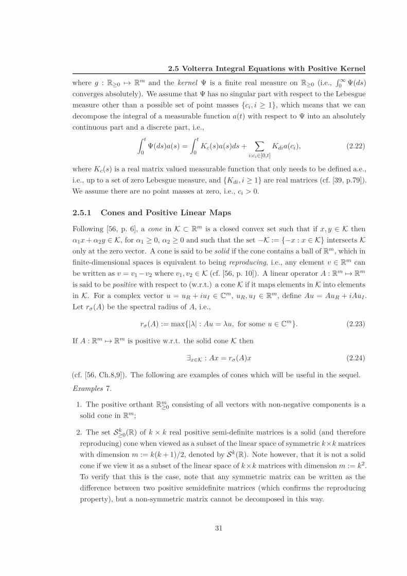
2.5 Volterra Integral Equations with Positive Kernel
where g : R$0 ,- Rm and the kernel $ is a finite real measure on R$0 (i.e.," %
0 $(ds)converges absolutely). We assume that $ has no singular part with respect to the Lebesguemeasure other than a possible set of point masses {ci, i " 1}, which means that we candecompose the integral of a measurable function a(t) with respect to $ into an absolutelycontinuous part and a discrete part, i.e.,
) t
0$(ds)a(s) =
) t
0Kc(s)a(s)ds +
*
i:ci&[0,t]Kdia(ci), (2.22)
where Kc(s) is a real matrix valued measurable function that only needs to be defined a.e.,i.e., up to a set of zero Lebesgue measure, and {Kdi, i " 1} are real matrices (cf. [39, p.79]).We assume there are no point masses at zero, i.e., ci > 0.
2.5.1 Cones and Positive Linear Maps
Following [56, p. 6], a cone in K 4 Rm is a closed convex set such that if x, y + K then$1x + $2y + K, for $1 " 0, $2 " 0 and such that the set 0K := {0x : x + K} intersects Konly at the zero vector. A cone is said to be solid if the cone contains a ball of Rm, which infinite-dimensional spaces is equivalent to being reproducing, i.e., any element v + Rm canbe written as v = v1 0v2 where v1, v2 + K (cf. [56, p. 10]). A linear operator A : Rm ,- Rm
is said to be positive with respect to (w.r.t.) a cone K if it maps elements in K into elementsin K. For a complex vector u = uR + iuI + Cm, uR, uI + Rm, define Au = AuR + iAuI .Let r"(A) be the spectral radius of A, i.e.,
r"(A) := max{|"| : Au = "u, for some u + Cm}. (2.23)
If A : Rm ,- Rm is positive w.r.t. the solid cone K then
3x&K : Ax = r"(A)x (2.24)
(cf. [56, Ch.8,9]). The following are examples of cones which will be useful in the sequel.Examples 7.
1. The positive orthant Rm$0 consisting of all vectors with non-negative components is a
solid cone in Rm;
2. The set Sk$0(R) of k # k real positive semi-definite matrices is a solid (and therefore
reproducing) cone when viewed as a subset of the linear space of symmetric k#k matriceswith dimension m := k(k + 1)/2, denoted by Sk(R). Note however, that it is not a solidcone if we view it as a subset of the linear space of k#k matrices with dimension m := k2.To verify that this is the case, note that any symmetric matrix can be written as thedi!erence between two positive semidefinite matrices (which confirms the reproducingproperty), but a non-symmetric matrix cannot be decomposed in this way.
31
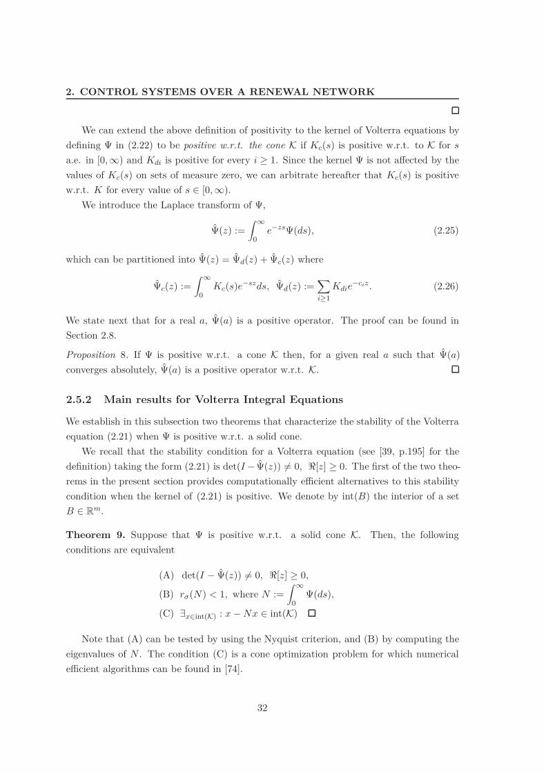
2. CONTROL SYSTEMS OVER A RENEWAL NETWORK
We can extend the above definition of positivity to the kernel of Volterra equations bydefining $ in (2.22) to be positive w.r.t. the cone K if Kc(s) is positive w.r.t. to K for s
a.e. in [0, /) and Kdi is positive for every i " 1. Since the kernel $ is not a!ected by thevalues of Kc(s) on sets of measure zero, we can arbitrate hereafter that Kc(s) is positivew.r.t. K for every value of s + [0, /).
We introduce the Laplace transform of $,
$(z) :=) %
0e!zs$(ds), (2.25)
which can be partitioned into $(z) = $d(z) + $c(z) where
$c(z) :=) %
0Kc(s)e!szds, $d(z) :=
*
i$1Kdie
!ciz. (2.26)
We state next that for a real a, $(a) is a positive operator. The proof can be found inSection 2.8.
Proposition 8. If $ is positive w.r.t. a cone K then, for a given real a such that $(a)converges absolutely, $(a) is a positive operator w.r.t. K.
2.5.2 Main results for Volterra Integral Equations
We establish in this subsection two theorems that characterize the stability of the Volterraequation (2.21) when $ is positive w.r.t. a solid cone.
We recall that the stability condition for a Volterra equation (see [39, p.195] for thedefinition) taking the form (2.21) is det(I 0 $(z)) 1= 0, %[z] " 0. The first of the two theo-rems in the present section provides computationally e"cient alternatives to this stabilitycondition when the kernel of (2.21) is positive. We denote by int(B) the interior of a setB + Rm.
Theorem 9. Suppose that $ is positive w.r.t. a solid cone K. Then, the followingconditions are equivalent
(A) det(I 0 $(z)) 1= 0, %[z] " 0,
(B) r"(N) < 1, where N :=) %
0$(ds),
(C) 3x&int(K) : x 0 Nx + int(K)
Note that (A) can be tested by using the Nyquist criterion, and (B) by computing theeigenvalues of N . The condition (C) is a cone optimization problem for which numericale"cient algorithms can be found in [74].
32
2.5 Volterra Integral Equations with Positive Kernel
As a preliminary to prove Theorem 9 we state two lemmas both proved in Section 2.8.The first lemma establishes a monotone property for the spectral radius of the Laplacetransform of $. We recall that if $(a) converges absolutely for some real a then $(z)converges absolutely in the set {z + C : %[z] " a}(cf. [39, Ch.3,Th.8.2]).
Lemma 10. Suppose that $ is positive w.r.t. a solid cone K, and that $(a) convergesabsolutely for some a + R. Then for any z : %[z] " a, the following holds r"($(z)) !r"($(a)).
The second Lemma characterizes the geometric placement of the zeros of det(I 0 $(z)).
Lemma 11. Suppose that $ is positive w.r.t. a solid cone K, and that $(a) convergesabsolutely for some a + R. Then, if r"($(a)) " 1, there exists a1 " a with the followingproperties:
(i) a1 is the unique real number such that r"($(a1)) = 1,
(ii) det(I 0 $(a1)) = 0,
(iii) if z : det(I 0 $(z)) = 0 then %[z] ! a1.
Proof. (of Theorem 9)(B)5(A) Note that N = $(0). From Lemma 10, r"($(z)) ! r"($(0)) = r"(N) for everyz : %[z] " 0. This implies that if (B) holds, all the eigenvalues of $(z) have a modulusstrictly less than one, and therefore det(I 0 $(z)) cannot be zero in %[z] " 0, whichimplies (A).(A)5(B) If r"(N) = r"($(0)) " 1, from Lemma 11 we have that there exists some a1 " 0such that det(I 0 $(a1)) = 0, and therefore condition (A) does not hold at z = a1.(B)5(C) If r"(N) < 1 the system of equations
Nx 0 x = 0v
has a unique solution given by
x =+%*
k=0Nk(v),
which satisfies x + K if v + K due to the fact that N is a positive operator (since N = $(0)and due to Proposition 8). If v + int(K) then since x = v + w, where
w =+%*
k=1Nk(y) + K
and v + int(K), we have that x + int(K). In fact, since v + int(K) there exists an % suchthat
B# := {z : )z 0 v) < %} . K.
33

2. CONTROL SYSTEMS OVER A RENEWAL NETWORK
Thus the set {w + z, z + B#} is a ball of radius % centered at x which belongs to K since w
and z belong to K, and thus x + int(K).(C)5(B) If (C) holds, then x 0 Nx = v for some v + int(K), from which we conclude that,for each k " 1,
x 0k!1*
j=0N jv = Nkx + K.
This implies that )!k
j=0 N jv) ! c)x) (cf [56, p.37]). Letting k - / we conclude that!%
j=0 N jv converges which implies that it converges absolutely, a general fact in Banachspaces (as it is the case since K + Rm), and this implies that Nkv - 0 as k - /. Givenany w + K, there exists $ > 0 such that v 0 $w + K because v + int(K). Then
Nkv 0 $Nkw = Nk(v 0 $w) + K,
and hence Nkw - 0 as k - / because Nkv - 0 as k - / and )$Nkw) ! c)Nkv).Finally, since K is reproducing, for every u + Rm, there exists u1, u2 + K such thatu = u1 0 u2, and therefore Nku = Nku1 0 Nku2 - 0 as k - /, which implies thatr"(N) < 1.
The Lyapunov exponent of the Volterra equation (2.21) is defined as follows.
Definition 12. Suppose that the solution to (2.21) satisfies )y(t)) 1= 0, 2t$0. Then thesecond order Lyapunov exponent for (2.21) is defined as
"V := limt'%
1t
log )y(t)) (2.27)
when such limit exists. Moreover, if 3b>0 : )y(t)) = 0, 2t > b then "V :=0/.
The next Theorem provides a method to determine the Lyapunov exponent "V for (2.21).Recall that a singularity zi of a complex function is said to be removable if the function isbounded in a neighborhood of zi. Consider the following assumptions.
(V1) $(0%) converges absolutely for some % > 0.
(V2) infz&C(R,#){| det(I0$d(z))|}>0 for some % > 0, andR > 0, where C(R, %) := {z : |z| > R, %[z] > 0%}.
(V3) g is bounded and g(t) = 0, t + [b, /) for some b > 0.
The same arguments utilized in the proof of Proposition 5 can be used to prove thatr"($d(0)) < 1 implies (V2), provided that (V1) holds.
34

2.5 Volterra Integral Equations with Positive Kernel
Theorem 13. Suppose that $ is positive w.r.t. a solid cone K and suppose that (V1),(V2) and (V3) hold, $(a) converges absolutely for some real a and r"($(a)) " 1. Thenthere is a unique
" > a : r"($(")) = 1 (2.28)
which is a singularity of [I0$(z)]!1g(z), and, if it is not removable, the Lyapunov exponent"V is given by "V = ". Moreover, if there does not exists a real a such that r"($(a)) " 1,then "V = 0/.
Note that r"($(a)) is a non-increasing function of a (cf. Lemma 10), and therefore (2.28)can be easily computed by performing a binary search.
To prove the Theorem 13 we need to derive two results. The first states how a specialperturbation of g(t) and $ a!ects the solution of (2.21). We introduce the following Laplacetransforms
y(z) :=) %
0y(s)e!zsds, g(z) :=
) %
0g(s)e!zsds. (2.29)
The following proposition can be obtained by direct substitution.
Proposition 14. Let g%(t) := g(t)e%t and $% be a measure such that,) t
0$%(ds)a(s) =
) t
0Kc(s)e%sa(s)ds +
*
i:ci&[0,t]Kdie
%cia(ci), (2.30)
for a measurable function a(t), where Kc and Kdi are specified by (2.22). Then the solutionto
y%(t) =) t
0$%(ds)y%(t 0 s) + g%(t), t " 0 (2.31)
satisfies y%(t) = y(t)e%t. Moreover
y%(z) = y(z 0 (), g%(z) = g(z 0 (), $%(z) = $(z 0 (), (2.32)
where y%(z), g%(z), and $%(z) are the Laplace transforms of w% and g% and $% defined asin (2.25) and (2.29).
The second is an instability result that takes into account the critical case, i.e, it allowsthe characteristic equation (det(I 0 $(z)) = 0)) to have zeros on the imaginary axis. It isimportant to emphasize that this result avoids the hard-to-test assumptions typically usedto handle the critical case (e.g. [39, Ch.7,Th.3.7]).
Lemma 15. Consider a general Volterra equation taking the form (2.21) and suppose that(V1), (V2), (V3) hold. Then
(i) there exists at most a finite number of zi + C such that %[zi] " 0 and det(I 0$(zi)) =0.
35

2. CONTROL SYSTEMS OVER A RENEWAL NETWORK
(ii) The solution to (2.21) is given by
y(t) = ws(t) +nz*
i=1
mi!1*
j=0si,jt
jezit, t " 0, (2.33)
and its Laplace transform is given by y(z) = [I 0 $(z)]!1g(z), where ws(t) is abounded function that converges to zero and si,j are such that in a neighborhoodof zi,
y(z) = ui(z) +mi!1*
j=0si,j
j!(z 0 zi)j+1 , (2.34)
where ui(z) are analytic vector functions.
The proof of Lemma 15 is given in Section 2.8. Note that the second term on the righthand side of (2.34) is the principal part of y(z) at zi and si,j can be uniquely determinedby the characterization (2.34) (see [80, Ch.10, Th.10.21]).
Proof. (of Theorem 13)If there exists a real number a such that r"($(a)) " 1, then there exists a unique " + R
such that r"($(")) = 1, which satisfies det(I 0 $(")) = 0 (cf. Lemma 11), and therefore "
is a singularity of [I 0$(z)]!1g(z). Consider a perturbation to the Volterra equation (2.21)as in Proposition (14) with ( = 0". Since " is the zero of det(I 0 $(z)) with largest realpart (cf. Lemma 10), we have that z1% = 0 is the zero of det(I 0 $%(z)) = det(I 0 $(z 0 ())with largest real part, where we used (2.32). Also, due to (2.32), the principal parts of y(z)about zi and of y%(z) about zi + ( have the same coe"cients si,j. Thus, from Lemma 15,the solution to the Volterra equation (2.31) becomes y%(t) = v%(t) + u%(t) + w%(t) wherev%(t) = !mi!1
j=0 s1,jtj corresponds to the zero of det(I 0 %(z)) labeled z1% = 0, u% is a sumof exponent and polynomial functions such that u%(t)e!ct - 0, as t - / for every c > 0and w%(t) is a bounded function that converges to zero. Note that u% may not tend to zerosince there may exist zeros of det(I 0 %%(z)) on the imaginary axis other than z1%. Sincethe singularity z1 = " is not removable, 3j : s1,j 1= 0, we have that y(t) = y%(t)e!%t is suchthat
"V = limt'%
log()y(t)))t
= limt'%
log()y%(t)))t
0 ( =00( =".
If there does not exists a real number a such that r"($(a)) " 1, then using Lemma 10, wehave that r"($(z)) < 1 for every complex z and therefore det(I 0%(z)) 1= 0 for all z. Usingthe arguments above we can choose ( arbitrarily large, and prove that y(t) = y%(t)e!%t
where y%(t) is a bounded function that converges to zero. This implies that &V = 0/. Notethat, this latter case encompasses the case where, e.g., $([0, t]) = 0, 2t$0 and y(t) = g(t)is such that y(t) = 0, t > b for some b > 0.
36

2.6 Proofs of the Main Results
2.6 Proofs of the Main Results
As a preliminary, we rewrite (2.19) in two forms. Applying '!1 to both sides of (2.19),and using (2.14), we obtain
W (t) = K(W )(t) + H(t), t " 0 (2.35)
where W (t) := '!1(w(t)), H(t) :=eA!tXeAtr(t) and
K(W )(t) :=) t
0(JeAs)!W (t 0 s)JeAsµ(ds).
Let Kj(W )(t) denote the composition operator obtained by applying j times K. Theunique solution to (2.35) is given by
W (t) =%*
j=1Kj(H)(t) + H(t), t " 0, (2.36)
(cf. [39, Ch.4, Th.1.7]). Note that H(t) and K(H)(t) are symmetric and therefore W (t) issymmetric. Let {Ci, 1 ! i ! m}, with m := n(n+1)
2 , be an orthogonal basis for the spaceof symmetric matrices Sn(R) and let '(x) : Rm ,- Sn(R) be the invertible map defined by
'(x) =m*
i=1xiCi.
Then (2.35) (or equivalently (2.19)) can be written in terms of u(t) := '!1(W (t)) as
u(t) =) t
0%(ds)u(t 0 s) + e(t) (2.37)
where e(t) = '!1(H(t)) and %(ds) is such that) t
0%(ds)a(s) =
) t
0Fc(s)a(s)ds +
*
i:ci&[0,t]Fdia(ci)
where a(s) is a measurable function and
Fc(s) = '!1'!1(JeAs)! $ (JeAs)!f(s)'',
Fdi = '!1'!1wi(JeAbi)! $ (JeAbi)!''.(2.38)
The kernel % is positive w.r.t. the cone in Rm corresponding to Sk$0(R), i.e., KS := {v +
Rm : !mi=1 viCi > 0}. In fact, if x + KS , i.e., X = '(x) " 0 then using (2.38) and (2.15)
Fc(s)x = '!1(Y ) + KS , where Y = (JeAs)!XJeAsf(s).
Similarly one can prove that all the Fdi are positive operators.
37
2. CONTROL SYSTEMS OVER A RENEWAL NETWORK
Let %(z) :=" %
0 e!zs%(ds). Since % is a positive kernel w.r.t. the solid cone KS
(cf. Example 7.2), from Theorem 9 we obtain that the following are equivalent:
(A’) det(I 0 %(z)) 1= 0, %[z] " 0,
(B’) r"(%(0)) < 1,
(C’) 3x&int(KS) : x 0 %(0)x + int(KS).
We shall also need the following facts: Using (2.38), we have
%(z) = '!1'!1#(z)''. (2.39)
Since % is positive w.r.t. a solid cone we have that %(a) for real a is a positive operator(cf. Proposition 8), and therefore from (2.24),
3x&KS : %(a)x = r"(%(a))x (2.40)
which, using (2.39), can be written as
3X$0#(a)'(X) = r"(%(a))'(X). (2.41)
Proof. (of Theorem 3)Since, as discussed above, (A’)-(C’) are equivalent, to prove that (A)-(C) are equivalent
we can show that
(C) 6 (C’) , (C) 5 (B), (B) 5 (A), (A) 5 (A’).
(C)6(C’) Using (2.39) with z = 0 we write (C’) as
3P >0 : '(P ) 0 M'(P ) + {'(Q) : Q > 0}. (2.42)
Applying '!1 to (2.42), and using (2.15), we conclude that (2.42) is equivalent to (C).(C) 5(B) Let Sn
$0(C) be the set of n # n complex positive semi-definite matrices andconsider the system
uk+1 =M!uk, Uk+1 =L)(Uk), '(Uk)=uk, U0 + Sn$0(C), (2.43)
where L)(Uk) := '!1 7 M! 7 '(Uk) is given by
L)(Uk) =) T
0JeAsUk(JeAs)!F (ds),
and for any Y, Z + Sn+(C) satisfies
tr(L(Z)"Y ) = tr(Z"L)(Y )). (2.44)
38

2.6 Proofs of the Main Results
Note that Uk " 0 for a given k implies that Uk+1 = L)(Uk) " 0, and therefore, by induction,we conclude that Uk " 0 for all k. We show that (C) implies that this system is stable byconsidering a Lyapunov function
V (uk) := tr(P'!1(uk))
for (2.43), where P satisfies (C), that is P > 0 and L(P ) 0 P < 0. In fact, this function V
is radially unbounded and positive definite for Uk " 0, and satisfies V (0) = 0. Using (C)and (2.44) we have that for every Uk + Sn
$0(C) 0 {0},
V (uk+1) 0 V (uk) = tr(P'!1(M!'(Uk))) 0 tr(PUk)= tr(PL)(Uk))0tr(PUk)= tr((L(P )0P )Uk)= 0tr(ZUk) < 0,
where Z := 0(L(P ) 0 P ) > 0. Therefore (2.6) is stable for any U0 + Sn$0(C), i.e.,
(M!)kU0 - 0. Since any complex matrix Z can be written as
Z = Z1 0 Z2 + i(Z3 0 Z4),
where Zi + Sn$0(C), 1 ! i ! 4 (cf. [57, Rem. 2]) this implies that (M!)kZ - 0, which
implies thatr"(M) = r"(M!) < 1.
(B)5(A) For z : %[z] " 0 and X, Y + Sn$0(C), we have
|'Y, '!1(#k(z)'(X))(|
= |) T
0. . .
) T
0tr(Y "(JeAhk )!. . . (JeAh1)!XJeAh1 . . . JeAhk e!zh1 . . . e!zhkµ(dh1) . . . µ(dhk)|
!) T
0. . .
) T
0|tr(Y "(JeAhk )!. . . (JeAh1)!X(JeAh1) . . . JeAhk |µ(dh1) . . . µ(dhk)
= 'Y, '!1(Mk'(X))( (2.45)
where the last equality holds because tr(Y "(JeAhk)!. . . (JeAh1)!XJeAh1 . . . JeAhk) is a non-negative function since it can be written as the inner product of two (complex) positivesemi-definite matrices. If (B) holds then r"(M) < 1, Mk'(X) converges to zero as k tendsto infinity and by the inequality (2.45) this implies that |'Y, '!1(#k(z)'(X))(| convergesto zero for any matrices Y, X + Sn
$0(C). Given Z1, Z2 + Cn#n we can write Zj = Zj1 0
Zj2 + i(Zj
3 0 Zj4), where for 1 ! l ! 4 and 1 ! j ! 2, Zj
l + Sn$0(C) (cf. [57, Rem. 2]). Thus,
|'Z1, '!1(#k(z)'(Z2))(| !*
1*l*4,1*j*2clj |'Zj
l , '!1(#k(z)'(Zjl ))(|
39
2. CONTROL SYSTEMS OVER A RENEWAL NETWORK
also converges to zero as k tends to infinity, where clj are constants. This implies r"(#(z)) <
1 in %[z] " 0 and thus det(I 0 #(z)) cannot be zero in %[z] " 0, which is (A).(A) 5 (A’) If (A)) does not hold then there must exist a z1 : %[z1] " 0 such that det(I 0%(z1)) = 0 and this implies that
3x&Cm : %(z)x = x. (2.46)
Using (2.39) we conclude that (2.46) can be rewritten as
3X=Y +iZ:Y,Z&Sn(R) : #(z1)'(X) = '(X)
and this implies thatdet(I 0 #(z1)) = 0,
which means that (A) does not hold.
Su!ciency of (A) and (2.8), (2.9), (2.10) for MSS, SS and MES
We start by noticing that (2.8) is equivalent to h(t) (or H(t)) converges to zero, and (2.9)is equivalent to
" T0 h(t)dt (or
" T0 H(t)dt) converging absolutely. Moreover, since
E[x(t)!x(t)] = x!0 $ x!
0w(t) = x!0W (t)x0,
where W (t), given by (2.36), is non-zero and positive semi-definite, MSS is equivalentto w(t) - 0 (or W (t) - 0), SS is equivalent to
" %0 w(t)dt (or
" %0 W (t)dt) converges
absolutely.Su"ciency of conditions (A) and (2.8) for MSS and of conditions (A) and (2.9) for SS
follow then directly from [39, Ch.4,Th.4.9], which states that for a Volterra equation takingthe form (2.19) if
inf([z]$0
| det(I 0 #(z))| > 0
then, w(t) is bounded and converges to zero if h(t) is bounded and converges to zero," %
0 w(t)dt converges absolutely if" %
0 h(t)dt converges absolutely. It remains to prove thatinf | det(I 0 #(z))| > 0 for z in %[z] " 0 is equivalent to det(I 0 #(z)) 1= 0 in the samecomplex region. Necessity is trivial. To prove su"ciency note that, det(I 0 #(z)) 1= 0in %[z] " 0 is equivalent to r"(#(0)) < 1, due to the equivalence between (A) and (B)of the present theorem. If r"(#(0)) < 1, then by Lemma 10, r"(#(z)) < 1 in the closedright half plane and therefore inf(| det(I 0 #(z))|) > 0 in %[z] " 0. To prove su"ciency ofthe conditions (A) and (2.10) for MES, we use a perturbation as in Proposition 14. For( < min(%, $1) where % is such that (T1) holds and $1 is such that (2.10) holds, we obtainthat h%(t) = h(t)e%t, and #%, satisfy the conditions (A) and (2.8) of the present theorem
40

2.6 Proofs of the Main Results
for MSS and therefore w%(t) converges to zero, whereas w(t) = w%(t)e!%t converges to zeroexponentially fast.
Necessity of (A) and (2.8), (2.9), (2.10) for MSS, SS and MES
From (2.36), W (t) " H(t). Hence, W (t) - 0 (MSS)," %
0 W (t)dt converges absolutely(SS), and W (t) converges to zero exponentially fast (MES), imply that the respectivecondition must hold for H(t) (or equivalently for h(t)) and therefore that (2.8), (2.9),and (2.10) must hold, respectively. Necessity of (A) for MSS, SS and MES, follows fromLemma 15, which requires (V1) and (V2), implied by (T1) and (T2), and also (V3), whichis assumed for now to hold, i.e., h(t) = 0, 2t>b for some b > 0, which holds for example if µ
has bounded support. If (A) does not hold, from Lemma 11 there exists a real a > 0 suchthat det(I 0 #(a)) = 0. Thus, from Lemma 15, w(t) converges to infinity exponentiallyfast, since the zero zi = a is not a removable singularity (3j : si,j " 0 (cf. Proof ofTheorem 4). If (V3) does not hold, we can use a similar reasoning to prove that (A) isnecessary for MSS, SS, and MES. Let W2(t) be the solution to (2.35) when H(t) is replacedby H2(t) := H(t) if t > b, H(t) := 0 otherwise for some b > 0. Then, W2(t) ! W (t) since
W (t) 0 W2(t) = K(W 0 W2)(t) + H(t) 0 H2(t),
whose solution is positive semi-definite (cf. (2.36)). Thus, since (A) is necessary for W2(t)to be MSS, SS and MES, it is also for W (t).
Proof. (of Theorem 4) Note that
E[x(t)!x(t)] = (x!0 $ x!
0)w(t) = x!0W (t)x0 =
m*
i=1ui(t)x!
0Cix0.
Note also that )W (t)) = )w(t)) = )u(t)). It is then clear that the limit
"L(x0) = limt'%
1t
log(E[x(t)!x(t)])
exists for every x0 if and only if the limit "V = limt'%1t log()u(t))) exists, and "V =
supx0 "L(x0) = "L. Note also that E[x(t)!x(t)] = 0, 2x0 , t > b > 0 if and only if u(t) =0, t > b > 0 in which case both "L and "V equal 0/ according to our definitions. We useTheorem 13 applied to the Volterra equation (2.37) to obtain that "V is determined byr"($("V )) = 1, when such a "V exists, and "V = 0/ otherwise. Note that "L in (2.11)equals "V since we can obtain that r"(%(a)) = r"(#(a)), for real a such that %(a) and #(a)converge. In fact, similarly to the equivalence between (B’) and (B) established in the proofof Theorem 4, we can prove that r"(%(a)) < 1 is equivalent to r"(#(a)) < 1, for every reala such that %(a) and #(a) converge, which implies that r"(#(a)) = r"(%(a)). To apply
41

2. CONTROL SYSTEMS OVER A RENEWAL NETWORK
Theorem 13, we note that the the fact that µ has bounded support implies conditions (T1)and (T2), which in turn, imply (V1) and (V2). Moreover, the fact that µ has boundedsupport implies (V3). It su"ces to prove that the real zero a of det(I 0 %(a)) such thatr"(%(a)) = 1, is not a removable singularity of R(a)e(a) where R(a) := [I 0 %(a)]!1 ande(z) :=
" %0 e(t)e!ztdt is the Laplace transform of e(t).
To this e!ect, we start by noticing that, using (2.40),
3x&KS : %(a)x = x (2.47)
which, by using (2.39), can be written as
3X$0La(X) = X, (2.48)
whereLa(X) :=
) %
0(JeAs)!X(JeAs)e!asµ(ds).
LetH(b) :=
) %
0eA!teAtr(t)e!btdt
and note that there exists $ such that $X ! H(b). For b > a, r"(%(b)) < 1 due to thecharacterization of a of Lemma 10 and due to the monotonicity property of Lemma 11.Thus, we can expand R(b) as a von Neumann series and conclude that
R(b)e(b) =%*
k=0%(b)ke(b) =
%*
k=0'[Lk
b (H(b))] "%*
k=0$'(Lk
b (X)), (2.49)
where Lkb denotes the composition of applying Lb, k times. Using (2.48), we have that
lima'b Lkb (X) = Lk
a(X) = X. This implies, taking the limit as b - a in (2.49), thatlimb'a,b>a R(b)e(z) cannot be finite and therefore a is not a removable singularity.
2.7 Additional Applications of Theorems 9 and 13
We can apply the results provided in Subsection 2.5.2 to other problems where Volterraequations arise and have the special property of having a positive kernel, e.g., in physics,engineering, biology (cf. [39, Ch.1]). As an example, consider the setup in Fig. 2.2. AnLTI system is defined by a convolution product v(t) = (H 8 e)(t) where e(t) + Rm is theinput, v(t) + Rm the output, H(t) = [hi,j ]m#m is the impulse response, and 8 denotesconvolution. All signals are defined for t " 0. The Laplace transform of H is given byH(z) :=
" %0 H(t)e!ztdt, and the closed loop is defined by e(t) = v(t) + r(t) for a reference
signal r(t), which leads to the following Volterra equation
v(t) =) t
0H(s)v(t 0 s)ds +
) t
0H(s)r(t 0 s)ds. (2.50)
42

2.8 Proofs of Auxiliary Results
Figure 2.2: MIMO LTI closed loop
The transfer function H is not rational, e.g., when the impulsive response H(t) exhibitsdelays. Following [39, Ch.1], we say that the closed-loop is stable if v(t) belongs to Lp (i.e.," t
0 |v(t)|pdt < /, if p < / and v(t) is bounded a.e. if p = /) whenever r(t) belongs to Lp.Assume that
" %0 H(t)dt converges absolutely which, in the case where H(z) is rational, is
equivalent to saying that the open-loop is stable. The stability of the closed-loop can betested by the condition
det(I 0 H(z)) 1= 0, 2z&([z]$0, (2.51)
One can conclude this from the stability condition for the Volterra equation (2.50) orfrom [39, Ch.4, Th.4.9]. However, when H(t), 2t is a positive operator w.r.t. a given coneK + Rm ( e.g., Rm
$0), we can use the following very simple algebraic test for stability.
Corollary 16. If hi,j(t) " 0 for every t " 0 and 1 ! i, j ! m, then the closed-loop describedby (2.50) is stable if and only if
r"(H(0)) < 1. (2.52)
Proof. Since H(t) is positive w.r.t the solid cone Rm$0, Theorem 3 assures that (2.52)
and (2.51) are equivalent.
2.8 Proofs of Auxiliary Results
Proof. (of Proposition 5) The condition (T1) assures that #d(y) converges absolutely fory > 0% and in this region, r"(#d(y)) is continuous (cf. [39, Ch. 3, Th.3.8]). Therefore,r"(#d(0)) < 1 implies that r"(#d(0%1)) < 1 for some %1 + (0, %), and from Lemma 10we have r"(#d(z)) < 1 in %[z] " 0%1, which encompasses C(%1, R), R > 0. This impliesinf | det(I 0 #d(z))| > 0 in C(%1, R).
Proof. (of Proposition 6) Conditioning (2.18) on the time of the first jump t1, we obtain
w(t) =) %
0E[T (t)! $ T (t)!'(I)|t1 = s]µ(ds). (2.53)
43

2. CONTROL SYSTEMS OVER A RENEWAL NETWORK
The integrand has a di!erent expression for s > t and s ! t,
E[T (t)! $ T (t)!'(I)|t1 = s]= (2.54)+,
-(eA!t $ eA!t)'(I), if s > t
E[(T1(t 0 s)JeAs)!$ (T1(t 0 s)JeAs)!'(I)], if s! t
where T1(t 0 s) is the transition matrix of (2.6) from s = t1 to t, which depends on{hk : k " 1}. Due to the i.i.d. assumption on the intervals between transitions E[T1(t)! $T1(t)!'(I)] = w(t). Thus, partitioning (2.53) using (2.54) we obtain (2.19):
w(t) =) t
0E[(T1(t 0 s)JeAs)!$ (T1(t 0 s)JeAs)!'(I)]µ(ds)+
) %
tE[(eA!t $ eA!t)'(I)]µ(ds)
=) t
0(JeAs)! $ (JeAs)!w(t 0 s)µ(ds) + (eA!t $ eA!t)'(I)r(t),
where we used the fact that we can write the first term on the right hand side of (2.19) as) t
0#(ds)w(t 0 s) =
) t
0(JeAs)! $ (JeAs)!w(t 0 s)µ(ds),
which can be concluded by extending [80, Ch.1, Th.1.29] to real matrix-valued measures.
Proof. (of Proposition 8) From the fact that
$(a) =) %
0Kc(s)e!asds +
*
i$1Kdie
!aci , (2.55)
it su"ces to prove that" %
0 Kc(s)e!asds is a positive operator since this implies that (2.55)is a sum of positive operators and therefore a positive operator. It is clear that the factthat $(a) converges absolutely implies that
" %0 Kc(s)e!asds converges absolutely. Since
the space of continuous function with bounded support on R$0, denoted by Cc, is dense inthe space of measurable function whose Lebesgue integral on R$0 is absolutely convergent,denoted by L1, (cf. [80, Th.3.14]), there exists a sequence Kn(s) + Cc such that
|) %
0(Kn(s) 0 Kc(s))e!asds| <
%n
2 ,
where %n - 0. Since Kn(s) is Riemann integrable, we can find a matrix step functionKR
n (s), and hn-spaced points si such that) %
0KR
n (s)e!asds =Nn*
i=1hnKR
n (si)e!asi .
The result of this integral is a positive operator since it is the sum of positive operators.Moreover for each n we can choose Nn su"ciently large such that
|) %
0(KR
n (s) 0 Kn(s))e!asds| <%n
2 .
44

2.8 Proofs of Auxiliary Results
Thus,|) %
0KR
n (s)e!asds0) %
0K(s)e!asds| < %n - 0, as n - /
and therefore" %
0 K(s)e!asds is a positive operator since it is the limit of positive operators,and the space of positive operators w.r.t a given cone is closed (cf. [56, p.22]).
Proof. (of the Lemma 10) By Proposition 8, $(a) is positive w.r.t. K, and by inductionso is $(a)k. Let v belong to the dual cone K" of K, i.e., the set v + Rm such that'x, v( " 0, 2x&K. Such v di!erent from zero always exists if K does not coincide with thewhole space [56, p.22]. For every v + K" and for real a, '$(a)kx, v( is a positive numberby definition of K". For z : %[z] " a and for every v + K", w + K and k " 1, one can showthat
|'$(z)kw, v(| ! '$(a)kw, v(. (2.56)
For example, for k = 2, let
a(r, s) := 'Kc(r)Kc(s)w, v(, bj(s) := 'Kc(s)Kdjw, v(
di(r) := 'KdiKc(r)w, v(, hij := 'KdiKdjw, v(
which are positive functions due to the fact that the kernel $ is positive and by definitionof K". Then
|'$(z)2w, v(| = |) %
0
) %
0a(r, s)e!zre!zsdrds +
) %
0
%*
j=1bj(s)e!zcj e!zsds+
) %
0
%*
i=1di(r)e!zcie!zrdr +
%*
i=1
%*
j=1hije!zcj e!zci |
!) %
0
) %
0|a(r, s)|e!are!asdrds +
) %
0
%*
j=1|bj(s)|e!acj e!asds+
) %
0
%*
i=1|di(r)|e!acie!ardr +
%*
j=1
%*
i=1|hij |e!acie!acj
= '$(a)2w, v(
where we used the fact that a(r, s), bj(s), di(r), hji are positive functions.If r"($(a)) < 1, then $(a)k converges to zero as k tends to infinity, and so does
'$(a)kw, v( for every v + K", w + K. Since K is solid, and therefore reproducing, so isK"(cf. [56, Th. 4.5] and use the fact that a cone in (Rm, ).)) is normal [56, p. 37]). Thus,for any u, y + Rm we can write u = u1 0 u2 and y = y1 0 y2, for ui + K, yi + K", i + {1, 2}and obtain that
|'$(z)ku, y(| !*
1*i,j*2|'$(z)kui, yi(|. (2.57)
45
2. CONTROL SYSTEMS OVER A RENEWAL NETWORK
Each of the terms on the right hand side of (2.57) tend to zero as k - / due to (2.56)and the fact that r"($(a)) < 1. This implies that '$(z)ku, y( - 0 for every u, y + Rm andtherefore that $(z)k -0 as k-/, which in turn implies that r"($(z))<1.
To conclude the proof we note that for $ > 0, if r"($(a)) < $ then r"( 1! $(a)) < 1.
Using the above arguments this implies that r"( 1! $(z)) < 1, for z : %[z] " a, or equivalently
that r"($(z)) < $. Since $ is arbitrary, r"($(z)) ! r"($(a)).
Proof. (of Lemma (11)) To prove (i), note first that, r"($(y)) is continuous along y " a
and converges to zero as y - +/. By the intermediate value theorem, if r"($(a)) "1 then 3a1$a : r"($(a1)) = 1. To see that a1 is the unique real number that satis-fies r"($(a1)) = 1, suppose that r"($(a2)) = 1 for another real number a2. Due toLemma 10, we must have r"($(y)) = 1 in y + [min{a1, a2}, max{a1, a2}]. Since, by theproperty (2.24), r"($(a1)) = 1 is an eigenvalue, this implies that det(I 0 $(y)) = 0, iny + [min{a1, a2}, max{a1, a2}]. But det(I 0 $(z)) = 0 is analytic and the zeros of analyticfunctions (other than the identically zero function) are isolated (cf. [80, Th.10.18]), whichleads to a contradiction.Since $(a) is a positive operator due to Proposition 8, by the prop-erty (2.24) of positive operators w.r.t. solid cones, r"($(a1)) = 1 is an eigenvalue and thisimplies that det(I 0 $(a1)) = 0 (part (ii)). Finally, we argue by contradiction to prove (iii).If there exists w satisfying %[w] > a1 and det(I 0 $(w)) = 0 then $(w) has an eigenvalueat 1 and therefore r"($(w)) " 1. From Lemma 10, r"($(w)) ! r"($(%[w])) which impliesthat r"($(%[w])) " 1. Now, r"($(%[w])) cannot be equal to one since a1 is the uniquereal number that satisfies this property and %[w] > a1. This leads to a contradiction since,again by Lemma 10, r"($(%[w])) ! r"($(a1)) = 1.
Proof. (of the Lemma 15)Theorems [39, Ch.7,Th.2.4,2.5] and the argument in [39, p.192] would allow us to
conclude that (i) and (ii) hold if:
infz:([z]=0
| det(I 0 $(z))| > 0, (2.58)
lim|z|'%,([z]$0
inf | det(I 0 $(z))| > 0, (2.59)
g(t) is bounded and converges to zero. (2.60)
Note that (2.58) is restrictive since det(I 0 $(z)) would not be allowed to have zeros orthe imaginary axis (critical case). It is clear that (V3) implies (2.60). Note also that (V2)implies (2.59) and, since we assume (V2), the condition (2.58) can be simply stated as thecharacteristic equation det(I 0 $(z)) = 0 has no zeros on the imaginary axis (non-criticalcase).
The proof of (i) under assumptions (V1), (V2) is a direct consequence of the argumentsin [39, p.192] and [39, p.195] are is therefore omitted. To prove (ii) under assumptions (V1),
46

2.9 Further Comments and References
(V2) and (V3) we argue as follows. Let g%(t) and $% be as in Proposition 14. Due to (2.32)the zeros of det(I 0 $%(z)) are given by zi + (, where zi are the zeros of det(I 0 $(z)). Ifdet(I 0 $(z)) has zeros on the imaginary axis (critical case), i.e., (2.58) does not hold, wecan always choose (due to part (i) of the present theorem) a ( : 0 < ( < %, where % is theconstant in (V1), and such that the characteristic equation of the Volterra equation (2.31)does not have zeros on the imaginary axis. Thus, the Volterra equation (2.31) satisfies theconditions (2.58), (2.59), (2.60) required by Theorems [39, Ch.7,Th.2.4,2.5] to assure (i)and (ii). Thus from Theorems [39, Ch.7,Th.2.4,2.5] one can conclude that
y%(t)=ys%(t)+nz*
i=1
mi!1*
j=0si,jt
je(zi+%)t+nw*
i=1
ni!1*
j=0qi,jt
jevit, (2.61)
where vi are the zeros of det(I 0$%(z)) in 0 < %[wi] < ( and we used the fact, due to (2.32),that the principal parts of y(z) about zi and of y%(z) about zi +( have the same coe"cientssi,j. Thus (2.33) follows from (2.61) due to y(t) = y%(t)e!%t.
2.9 Further Comments and References
Impulsive renewal systems are a special class of the piecewise deterministic processes con-sidered in [25]. In this chapter, we restricted ourselves to linear dynamic and reset maps.Impulsive renewal systems with general non-linear dynamic and reset maps are consideredin [44]. The paper [44] considers a more general class of impulsive systems in which the sys-tem evolves according to a stochastic di!erential equation between jumps (as opposed to adeterministic vector field). For this class of impulsive renewal systems, su"cient conditionsfor a form of exponential stability are provided.
Early work on systems with i.i.d. distributed parameters can be found in [4], [6], [59].The stability problems considered in these early references are typically cast into a discrete-time setting, even if the motivating stability problem is in a continuous-time setting, asit is the case for randomly sampled systems [59]. Su"cient conditions for continuous-time mean square stability are provided in [69] for impulsive renewal systems that arisein model-based networked control systems with stochastically spaced transmissions. Theapproach followed in [4], [6], [59], [69] involves a stability test in terms of a matrix eigen-value computation. An alternative approach that can be found in the literature to inves-tigate the stability of such systems resorts to stochastic Lyapunov functions, leading tostability conditions formulated in terms of the existence of a Lyapunov function satisfyingappropriate inequalities [32, 66]. We believe that the stability results (Theorems 3 and 4)that we obtain with our novel aproach cannot be obtained through any of the previousapproaches [44], [4], [6], [69], [32], [66]. Our stability result (Theorem 3 ) obviates the
47

2. CONTROL SYSTEMS OVER A RENEWAL NETWORK
conservativeness of the results in [44], [69] where only su"cient stability conditions arepresented to the case where the probability distributions of the intervals between reset canhave unbounded support. The stability tests in terms of an eigenvalue or an LMI com-putation resemble tests available for Markov linear systems [21], but, to the best of ourknowledge, a Nyquist test has not appeared previously for this type of systems.
Volterra integral equations arise in many problems in physics, engineering and biology.The excellent textbook [39] discusses an extensive number of results for these equations.The Volterra equation considered here has the special property that its kernel is a positiveoperator in a sense to be defined below. It is important to note that the notion of positive-ness needed in this chapter di!ers from the well-known notions of monotonicity (see [39,Ch.5]) and positiveness (see [39, Ch.16]).
The networked control setup is considered, e.g., in [44] and [87].
48

3
Network Features Modeled byFinite State Machines
In this chapter, we introduce Stochastic Hybrid Systems (SHSs) with renewal transitions,which are a generalization of impulsive renewal systems that allows one to considerablyaugment the number of networked control scenarios that one can model. In fact, withSHS with renewal transitions one can consider any scenario in which the network protocol,or more generally network features such as delays and packet drops, can be modeled bya finite state machine. In this chapter, we start by showing how one can model networkfeatures such as packet drops, round-robin protocols or delays, using finite state machines.
After presenting these networked control motivations, we formally define stochastichybrid systems with renewal transitions. Stated briefly, stochastic hybrid systems withrenewal transitions are systems with both continuous dynamics and discrete logic whoseexecution is specified by the dynamic equations of the continuous state, a set of rulesgoverning the transitions between discrete modes, and reset maps determining jumps ofthe state at transition times.
Besides defining this class of systems, which is an important generalization of impul-sive renewal systems, we provide results concerning the analyses of the transitory andasymptotic behavior of the statistical moments of a SHS with renewal transitions. First,we provide expressions for any moment of the SHS at a given time t in terms of a set ofVolterra equations. Note that in Chapter 2 we considered only a special second degreemoment for the special case of impulsive renewal systems. We discuss how by computingthe moments one can provide information about the probability density function of thestate of the SHS. For this latter problem, we highlight the advantages of our method whencompared to other general methods in the literature. The second main result provides amethod to obtain the Lyapunov exponents of even degree m, which are defined, in accor-dance to [66, p. 41], as the exponential decrease or increase rate at which the mth power
49

3. NETWORK FEATURES MODELED BY FINITE STATE MACHINES
of the norm of the state of the SHS, converges to zero or to infinity, respectively. We showthat when m is even, the Lyapunov exponents can be e"ciently determined by finding thezero of a monotonic function. As a corollary, we provide necessary and su"cient conditionsfor mean exponential stability, which is defined in terms of the exponential convergence tozero of the squared norm of the state of the SHS.
The remainder of the chapter is organized as follows. Examples of networked controlscenarios that can be modeled by finite state machines are given in Section 3.1. StochasticHybrid Systems are formally defined in Section 3.2, and our main results are provided inSection 3.3. A numerical example is provided in Section 3.4. The proofs of the main resultsare given in Section 3.5. Section 3.6 provides further comments and references.
3.1 Modeling Several Network Features by Finite State Ma-chines
We present next five networked control scenarios, where finite state machines are usedto model (i) static and round-robin protocols; (ii) delays; (iii) packet drops; (iv) nodesindependently accessing the same shared network; (v) nodes transmitting through morethan one renewal network. We will present a detailed study of scenarios (i) and (ii) andprovide numerical examples in Section 3.4. For the scenarios (iii), (iv), and (v), we onlybriefly sketch how they can be modeled by finite state machines. The finite state machinesmodeling NCS are loosely defined in this section by specifying the number and meaning ofdiscrete modes and specifying transitions in terms of events that trigger these transitions.In the next section, we formally introduce stochastic hybrid systems, which allow to rigor-ously model these descriptions. The ideas provided here can be used to model combinationsof these features (delays, packet drops, etc), when they occur simultaneously.
3.1.1 Round-Robin Protocols
Consider a networked control system for which a set of nodes consisting on sensors, actua-tors, and a controller, are connected through a communication network possibly shared byother users. The plant and controller are described by:
Plant: xP = AP xP + BP u, y = CP xP (3.1)Controller: xC =ACxC + BC y, u = CCxC + DC y. (3.2)
where u is the input to the plant, y is the input to the controller, y is the output of theplant, and u is the output of the controller. As explained in Section 2.1, it is typically thecase that one assumes that the controller has been designed to stabilize the closed-loop,when the process and the controller are directly connected, i.e., when u(t) = u(t), y(t) =
50
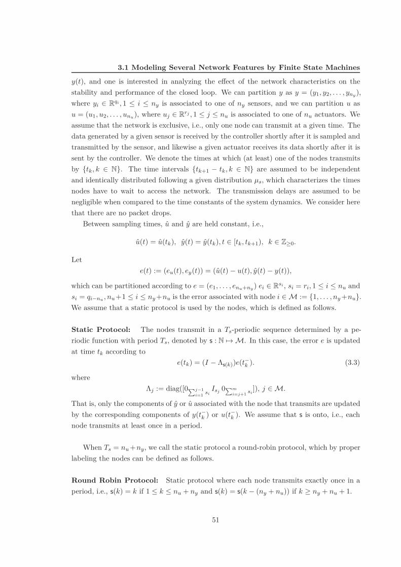
3.1 Modeling Several Network Features by Finite State Machines
y(t), and one is interested in analyzing the e!ect of the network characteristics on thestability and performance of the closed loop. We can partition y as y = (y1, y2, . . . , yny),where yi + Rqi , 1 ! i ! ny is associated to one of ny sensors, and we can partition u asu = (u1, u2, . . . , unu), where uj + Rrj , 1 ! j ! nu is associated to one of nu actuators. Weassume that the network is exclusive, i.e., only one node can transmit at a given time. Thedata generated by a given sensor is received by the controller shortly after it is sampled andtransmitted by the sensor, and likewise a given actuator receives its data shortly after it issent by the controller. We denote the times at which (at least) one of the nodes transmitsby {tk, k + N}. The time intervals {tk+1 0 tk, k + N} are assumed to be independentand identically distributed following a given distribution µs, which characterizes the timesnodes have to wait to access the network. The transmission delays are assumed to benegligible when compared to the time constants of the system dynamics. We consider herethat there are no packet drops.
Between sampling times, u and y are held constant, i.e.,
u(t) = u(tk), y(t) = y(tk), t + [tk, tk+1), k + Z$0.
Lete(t) := (eu(t), ey(t)) = (u(t) 0 u(t), y(t) 0 y(t)),
which can be partitioned according to e = (e1, . . . , enu+ny ) ei + Rsi, si = ri, 1 ! i ! nu andsi = qi!nu , nu +1 ! i ! ny +nu is the error associated with node i + M := {1, . . . , ny +nu}.We assume that a static protocol is used by the nodes, which is defined as follows.
Static Protocol: The nodes transmit in a Ts-periodic sequence determined by a pe-riodic function with period Ts, denoted by s : N ,- M. In this case, the error e is updatedat time tk according to
e(tk) = (I 0 &s(k))e(t!k ). (3.3)
where&j := diag([0!j!1
i=1 siIsj 0!m
i=j+1 si]), j + M.
That is, only the components of y or u associated with the node that transmits are updatedby the corresponding components of y(t!
k ) or u(t!k ). We assume that s is onto, i.e., each
node transmits at least once in a period.
When Ts = nu +ny, we call the static protocol a round-robin protocol, which by properlabeling the nodes can be defined as follows.
Round Robin Protocol: Static protocol where each node transmits exactly once in aperiod, i.e., s(k) = k if 1 ! k ! nu + ny and s(k) = s(k 0 (ny + nu)) if k " ny + nu + 1.
51

3. NETWORK FEATURES MODELED BY FINITE STATE MACHINES
Defining x := (xA, e), where xA := (xP , xc), the following system describes (3.1),(3.2),and (3.3),
#xA(t)e(t)
$
=#
I
Ae
$ %Axx Axe
& #xA(t)e(t)
$
(3.4)#xA(tk)e(tk)
$
=#I 00 (I 0 &s(k))
$ #xA(t!
k )e(t!
k )
$
, (3.5)
whereAxx =
#AP + BP DCCP BP CC
BCCP AC
$
,
Ae =#
0 0CC
0CP 0
$
, Axe =#BP BP DC
0 BC
$
.
This networked control scenario with static protocols can be modeled by a finite statemachine, specified as follows for the special case of a round-robin protocol.
Discrete modes. To model a NCS with a round-robin protocol as described above,we require nu + ny discrete modes, where each of these modes corresponds to thenode 1 ! i ! ny + nu having the transmission token, i.e., i is the node assignedto transmit when the network becomes available. At each discrete mode, x flowsaccording to (3.4).
Transitions. The times between transitions equal the network access time, dis-tributed according to µs. When a transition, corresponding to a transmission by nodei is triggered, the discrete mode changes from i to i + 1 for every 1 ! i ! nu + ny 0 1,and if i = nu + ny the next state equals i = 1. At each transition, x is updatedaccording to (3.5).
3.1.2 Delays
We start by modeling delays which may occur due to the times that users may have towait to access the network, and we continue to assume as in Section 3.1.1 that transmissiondelays are negligible. Another model for delays, more suitable to model transmission delays,is presented in Section 5.1.1. For simplicity, we consider only a single renewal network,where only one node transmits, as in Section 2.1, but the same ideas carry through to thecase where several nodes transmit through the network, as in Section 3.1.1.
Suppose that we wish to control a linear plant
xP (t) = AP xP (t) + BP u(t). (3.6)
52

3.1 Modeling Several Network Features by Finite State Machines
A state feedback controller taking the form KCxP (t) is implemented digitally and theactuation is held constant u(t) = u(s&), t + [s&, s&+1) between actuation update timesdenoted by {s&, ) " 0}.
The controller has direct access to the state measurements, but communicates with theplant actuators through a network possibly shared by other users. The controller attemptsto do periodic transmissions of data, at a desired sampling period Ts but these regulartransmissions may be perturbed by the medium access protocol. For example, users usingCSMA for medium access, may be forced to back-o! for a typically random amount oftime until the network becomes available. We assume these random back-o! times to bei.i.d. and denote by µs the associated probability measure.
We consider two di!erent cases:Case I: After waiting to obtain network access, the controller (re)samples the sensor,
computes the control law and transmits this most recent data. This case is the mostreasonable when transmitting dynamic data. Assuming that the transmission delays arenegligible, and defining x := (xP , u), we have
x = Ax, A =#AP BP
0 0
$
, (3.7)
x(sk) = Jx(s!k ), J =
#I 0
KC 0
$
. (3.8)
Since the intervals {sk+1 0 sk, k " 0} result from the controller waiting a fixed time Ts
plus a random amount of time with a measure µs(s), these intervals are independent andidentically distributed according to
µ'[0, !)
(=
+,
-µs(! 0 Ts), if ! " Ts
0, t + [0, Ts).(3.9)
This case is captured by the following simple finite state machine.
Discrete modes. A single discrete mode is required to model this scenario, in whichx flows according to (3.7).
Transitions. The times between transitions equal the network access times, dis-tributed according to (3.9). When a transition, corresponding to a transmission bynode i is triggered, the discrete mode remains unchanged and x is updated accordingto (3.8).
Case II: After waiting to obtain access to the network, the controller transmits thedata collected at the time it initially tried to transmit data. This case is more realisticthan Case I since the controller typically sends the sensor data to the network adapter and
53

3. NETWORK FEATURES MODELED BY FINITE STATE MACHINES
does not have the option to update this data at the transmission times. Let rk = sk + Ts,x := (xP , u, v) where v(t) := u&, t + [r&, r&+1) is a variable that holds the last computedcontrol value. We model this case by a finite state machine specified as follows
Discrete modes. Two modes are required to model this case.
– Mode 1- The controller waits for a fixed time Ts;– Mode 2- The controller waits a random time to gain access to the network.
Transitions. When in mode 1 the system transits to mode 2 at times r&. Thecorresponding state jump models the update of the variable v(r&) = u& that holdsthe last computed control value and is described by
x(r&) = J1,1x(r!& ), J1,1 =
0
112
I 0 00 I 0
KC 0 0
3
445 .
When in mode 2 the SHS transits to mode 1 at actuation update times s&. The statejump models the actuation update u(s&) = v(s!
& ) and is described by
x(s&) = J2,1x(s!& ), J2,1 =
0
112
I 0 00 0 I
0 0 I
3
445 .
The times spent in each mode can be modeled by reset-time measures given by
– Time spent in the discrete mode 1 follows a distribution µ1,1(!) = ((! 0 Ts),where ((! 0Ts) is the dirac measure, i.e., a discrete measure that places all masswi = 1 at time Ts.
– Time spent in the discrete mode 2 follows a distribution µ2,1(!) = µs(!).
In both discrete modes, the continuous-time dynamics are described by x = Aix,i + {1, 2}, A1 = A2 = A where
A =
0
112
AP BP 00 0 00 0 0
3
445 .
3.1.3 Other Networked Control Features
In the networked control scenarios that we have presented so far, we can see a trend whenmodeling networked control systems using an emulation approach. The model includes dif-ferential equations modeling plant and controller dynamics, and reset maps are introduced
54
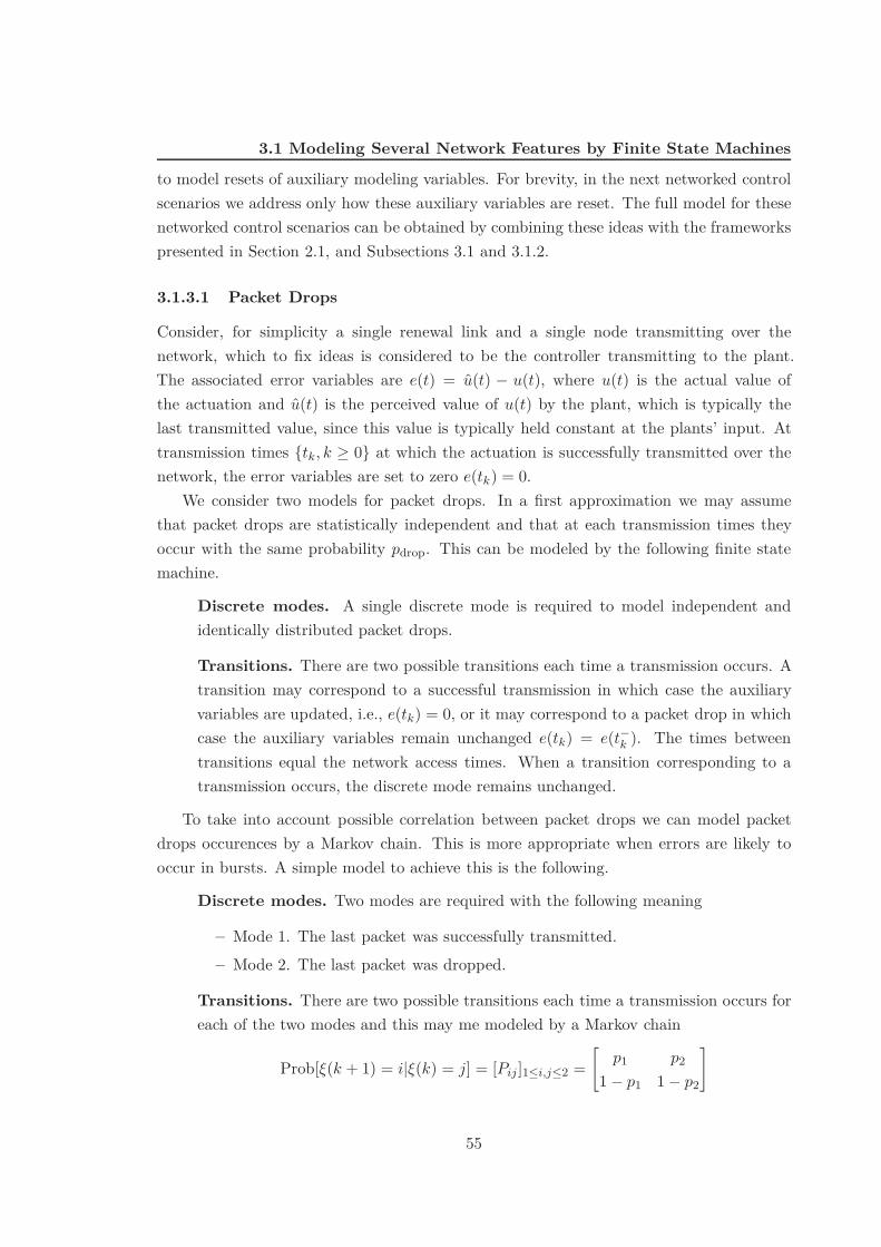
3.1 Modeling Several Network Features by Finite State Machines
to model resets of auxiliary modeling variables. For brevity, in the next networked controlscenarios we address only how these auxiliary variables are reset. The full model for thesenetworked control scenarios can be obtained by combining these ideas with the frameworkspresented in Section 2.1, and Subsections 3.1 and 3.1.2.
3.1.3.1 Packet Drops
Consider, for simplicity a single renewal link and a single node transmitting over thenetwork, which to fix ideas is considered to be the controller transmitting to the plant.The associated error variables are e(t) = u(t) 0 u(t), where u(t) is the actual value ofthe actuation and u(t) is the perceived value of u(t) by the plant, which is typically thelast transmitted value, since this value is typically held constant at the plants’ input. Attransmission times {tk, k " 0} at which the actuation is successfully transmitted over thenetwork, the error variables are set to zero e(tk) = 0.
We consider two models for packet drops. In a first approximation we may assumethat packet drops are statistically independent and that at each transmission times theyoccur with the same probability pdrop. This can be modeled by the following finite statemachine.
Discrete modes. A single discrete mode is required to model independent andidentically distributed packet drops.
Transitions. There are two possible transitions each time a transmission occurs. Atransition may correspond to a successful transmission in which case the auxiliaryvariables are updated, i.e., e(tk) = 0, or it may correspond to a packet drop in whichcase the auxiliary variables remain unchanged e(tk) = e(t!
k ). The times betweentransitions equal the network access times. When a transition corresponding to atransmission occurs, the discrete mode remains unchanged.
To take into account possible correlation between packet drops we can model packetdrops occurences by a Markov chain. This is more appropriate when errors are likely tooccur in bursts. A simple model to achieve this is the following.
Discrete modes. Two modes are required with the following meaning
– Mode 1. The last packet was successfully transmitted.– Mode 2. The last packet was dropped.
Transitions. There are two possible transitions each time a transmission occurs foreach of the two modes and this may me modeled by a Markov chain
Prob[*(k + 1) = i|*(k) = j] = [Pij ]1*i,j*2 =#
p1 p21 0 p1 1 0 p2
$
55

3. NETWORK FEATURES MODELED BY FINITE STATE MACHINES
where *(k) + {1, 2} denotes the mode of the finite state machine and k indexes trans-missions. If in mode 1, when a successful transmission occurs the discrete moderemains 1 and the auxiliary variables are updated, i.e., e(tk) = 0, and when a trans-mission is dropped the discrete mode is reset to 2 and the auxiliary variables remainunchanged e(tk) = e(t!
k ). Typically, when the last packet was successfully transmit-ted, one associates a high probability of a successful transmission occurring next, i.e.,p1 is typically close to one. If in mode 2, when a successful transmission occurs thediscrete mode is reset to 2 and the auxiliary variables are updated, i.e., e(tk) = 0.,and when a transmission is dropped the discrete mode is reset to 2 and the the aux-iliary variables remain unchanged e(tk) = e(t!
k ). Typically, when the last packet wasdropped, one associates a high probability of a packet drop occurring next, since er-rors are likely to occur in bursts, i.e., p2 is typically close to zero. The times betweentransitions equal the network access times.
3.1.3.2 Nodes Independently Accessing the Same Network
Consider a networked control system in which a remote controller communicates with aplant through a single shared communication network. Instead of assuming that plantand controller implement a high-level protocol as a round-robin protocol introduced inSubsection (3.1.1), suppose that plant and controller operate independently. Thereforethey compete for the network in general with other network users. We assume that acarrier sense multiple access protocol for medium access is fair, in the sense that theprobabilities of the plant transmitting to the controller and of the controller transmittingto the plant are the same. The associated auxiliary error variables are eu(t) = u(t) 0 u(t),where u(t) is the actual value of the actuation and u(t) is the perceived value of u(t) bythe plant, and ey(t) = y(t) 0 y(t), where y(t) is the actual value of the measurementsand u(t) is the perceived value of y(t) by the controller. Transmission times are denotedby {tk, k " 0} and the error variables are set to zero eu(tk) = 0, ey(tk) = ey(t!
k ) if thecontroller gains the access to the network at tk and eu(tk) = 0, eu(tk) = eu(t!
k ) if the plantgains the access to the network at tk. We can model this scenario by a finite state machinewith stochastic transitions.
Discrete modes. A single discrete mode is required to model the case where plantand controller aim independently to transmit over the same network.
Transitions. There are two possible transitions each time a transmission occurs attk and both have the same probabilities of occurring. Whether the plant gain accessto the controller and transmits to the plant, in which case eu(tk) = 0, ey(tk) = ey(t!
k ),or the controller gains access to the network and transmits to the plant, in which
56

3.2 Stochastic Hybrid Systems with Renewal Transitions
case eu(tk) = 0, ey(tk) = ey(t!k ). The times between transitions equal the network
access times.
3.1.3.3 Several Renewal Networks
Consider now a networked control system in which a remote controller communicates with aplant through two communication links; e.g., the actuation data is sent from the controllerto the plant through a shared wired network and the sensor data is sent from the plant tothe controller through a shared wireless network. The key point here is that these networkshave in general access times with di!erent distributions. Let ey, eu and tk have the samemeaning as in Subsection 3.1.3.2. If we assume that controller implement a (high-level)protocol with the plant, upon which they decide to transmit in a round-robin fashion, wecan model this scenario by the following finite state machine.
Discrete modes. Two modes are required with the following meaning.
– -Mode 1. The plant has the transmission token.
– -Mode 2. The controller has the transmission token.
Transitions. When in mode 1, a transition occurs to mode 2. The time spent inmode 1 corresponds to the time the plant takes to access the network from which ittransmits to the controller. When in mode 2, a transition occurs to mode 1. The timespent in mode 2 corresponds to the time the controller takes to access the networkfrom which it transmits to the plant, which is generally di!erently distributed fromthe access times of the network from which the plant transmits to the controller.
We can generalize these ideas to the case where several sensors and actuators transmitthrough di!erent, possibly many, networks. We shall consider the case where controllerand plant transmit independently and asynchronously in Chapter 4, in which case it doesnot appear to be possible to capture this scenario by a finite state machine.
3.2 Stochastic Hybrid Systems with Renewal Transitions
A SHS with renewal transitions, is defined by (i) a linear di!erential equation
x(t) = Aq(t)x(t), x(0) = x0, q(0) = q0, t0 = 0, (3.10)
where x(t) + Rn and q(t) + Q := {1, . . . , nq}; (ii) a family of n' discrete transition/resetmaps
(q(tk), x(tk)) = (*'(q(t!k )), Jq(t!
k ),'x(t!k )), + + L := {1, . . . , n'}, (3.11)
57

3. NETWORK FEATURES MODELED BY FINITE STATE MACHINES
where *' is a map *' : Q ,- Q and the matrix Jq(t!k ),' belongs to a given set {Ji,' + Rn#n, i +
Q, + + L}; and (iii) a family of reset-time measures
µi,', i + Q, + + L. (3.12)
Between transition times tk, the discrete mode q remains constant whereas the continuousstate x flows according to (3.10). At transition times, the continuous state and discretemode of the SHS are reset according to (3.11). The intervals between transition times areindependent random variables determined by the reset-time measures (3.12) as follows. Areset-time measure can be either a probability measure or identically zero. In the formercase, µi,' is the probability measure of the random time that transition + + L takes totrigger in the state q(t) = i + Q. The next transition time is determined by the minimumof the triggering times of the transitions associated with state q(t) = i + Q. Whenµi,'([0, s)) = 0, 2s$0, the transition + does not trigger in the state i + Q, which allows forsome reset maps not to be active in some states.
We assume that a transition probability measure µi,' can be decomposed as µi,' =µc
i,' + µdi,', with µc
i,'([0, t)) =" t
0 fi,'(s)ds, for some density function fi,'(s) " 0, and µdi,'
is a discrete measure that captures possible point masses {bri,' > 0, r " 1} such that
µdi,'({br
i,'}) = wri,'. The integral with respect to the measure µi,' is defined as
) t
0W (s)µi,'(ds) =
) t
0W (s)fi,'(s)ds +
*
r:bri,!&[0,t]
wri,'W (br
i,'). (3.13)
When the discrete measures µdi,' are di!erent from the zero measure, di!erent transitions
may trigger at the same time with probability di!erent from zero, leading to an ambiguityin choosing the next state. Thus, to guarantee that with probability one this does notoccur, we assume the following.
Assumptions 17.
(i) For every i + Q, the reset-time measures µi,', + + L for mode i have a finite numberof point masses;
(ii) For every i + Q, no two measures for mode i have common point masses, i.e., bji,l1
1=b&
i,l2 for l1 1= l2, l1 + L, l2 + L, 2j$1,&$1;
The construction of a sample path of the SHS with renewal transitions can be describedas follows.
1. Set k = 0, t0 = 0, (q(tk), x(tk)) = (q0, x0).
2. For every j + L, obtain hjk as a realization of a random variable distributed according
to µq(tk),j , if µq(tk),j is not identically zero, and set hjk = / otherwise.
58

3.2 Stochastic Hybrid Systems with Renewal Transitions
3. Takehk = min{hj
k, j + L} (3.14)
and set the next transition time to tk+1 = tk + hk. The state of the SHS in theinterval t + [tk, tk+1) is given by
(q(t), x(t)) = (q(tk), eAq(tk)(t!tk)x(tk)).
4. In the case where tk+1 < /, let lk denote the index of the transition that achievesthe minimum in step 3, i.e., lk = j : hk = hj
k and update the state according to(q(tk+1), x(tk+1)) = (*lk (q(t!
k+1)), Jq(t!k+1),lk x(t!
k+1)). Set k = k + 1 and repeat theconstruction from the step 2.
Due to the Assumption 17.(ii), there is zero probability that the minimum in step 3 isachieved by two or more indexes j.
3.2.1 Generalizations
Stochastic Hybrid Systems with renewal transitions are a special case of the stochastichybrid systems model presented in [45]. Two of the three generalizations discussed in [45]still apply to SHS with renewal transitions. We cannot model the case where discretetransitions are triggered by deterministic conditions on the state, e.g., guards being crossed,but we can generalize SHS with renewal transitions to the case where the dynamics aredriven by a Wiener process and the next state is chosen according to a given distribution,where the last generalization further requiring the transition distributions to be absolutelycontinuous. This latter generalization is especially useful to model the networked controlscenarios described in Sections 3.1.3.1 and 3.1.3.2, and therefore it is described next withmore detail.
Consider a dynamic system, which flows according to
x(t) = A1x(t), (3.15)
between transition times {tk, k " 0} at which the state is updated according to
x(tk) = J"k x(t!k ), (3.16)
where {,k, k " 0} are i.i.d. random variables with Prob[,k = 1] = p and Prob[,k = 2] =1 0 p. The intervals between transmissions {tk+1 0 tk, k " 0} are i.i.d. and are describedby a probability density function f , i.e., Prob[a ! tk+1 0 tk ! b] =
" ba f(s)ds, for b > a " 0.
An alternative characterization to f is given in terms of the survivor function of f , definedas
S(x) :=) %
xf(s)ds,
59
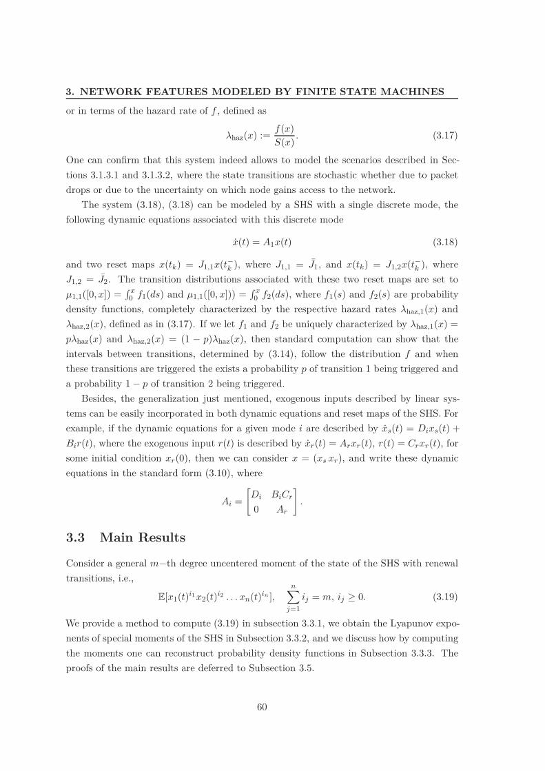
3. NETWORK FEATURES MODELED BY FINITE STATE MACHINES
or in terms of the hazard rate of f , defined as
"haz(x) := f(x)S(x) . (3.17)
One can confirm that this system indeed allows to model the scenarios described in Sec-tions 3.1.3.1 and 3.1.3.2, where the state transitions are stochastic whether due to packetdrops or due to the uncertainty on which node gains access to the network.
The system (3.18), (3.18) can be modeled by a SHS with a single discrete mode, thefollowing dynamic equations associated with this discrete mode
x(t) = A1x(t) (3.18)
and two reset maps x(tk) = J1,1x(t!k ), where J1,1 = J1, and x(tk) = J1,2x(t!
k ), whereJ1,2 = J2. The transition distributions associated with these two reset maps are set toµ1,1([0, x]) =
" x0 f1(ds) and µ1,1([0, x])) =
" x0 f2(ds), where f1(s) and f2(s) are probability
density functions, completely characterized by the respective hazard rates "haz,1(x) and"haz,2(x), defined as in (3.17). If we let f1 and f2 be uniquely characterized by "haz,1(x) =p"haz(x) and "haz,2(x) = (1 0 p)"haz(x), then standard computation can show that theintervals between transitions, determined by (3.14), follow the distribution f and whenthese transitions are triggered the exists a probability p of transition 1 being triggered anda probability 1 0 p of transition 2 being triggered.
Besides, the generalization just mentioned, exogenous inputs described by linear sys-tems can be easily incorporated in both dynamic equations and reset maps of the SHS. Forexample, if the dynamic equations for a given mode i are described by xs(t) = Dixs(t) +Bir(t), where the exogenous input r(t) is described by xr(t) = Arxr(t), r(t) = Crxr(t), forsome initial condition xr(0), then we can consider x = (xs xr), and write these dynamicequations in the standard form (3.10), where
Ai =#Di BiCr
0 Ar
$
.
3.3 Main Results
Consider a general m0th degree uncentered moment of the state of the SHS with renewaltransitions, i.e.,
E[x1(t)i1x2(t)i2 . . . xn(t)in ],n*
j=1ij = m, ij " 0. (3.19)
We provide a method to compute (3.19) in subsection 3.3.1, we obtain the Lyapunov expo-nents of special moments of the SHS in Subsection 3.3.2, and we discuss how by computingthe moments one can reconstruct probability density functions in Subsection 3.3.3. Theproofs of the main results are deferred to Subsection 3.5.
60
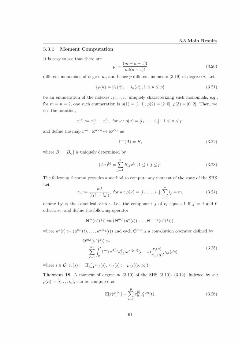
3.3 Main Results
3.3.1 Moment Computation
It is easy to see that there arep := (m + n 0 1)!
m!(n 0 1)! (3.20)
di!erent monomials of degree m, and hence p di!erent moments (3.19) of degree m. Let
{-()) = [i1()), . . . in())], 1 ! ) ! p} (3.21)
be an enumeration of the indexes i1 . . . , in uniquely characterizing such monomials, e.g.,for m = n = 2, one such enumeration is -(1) = [1 1], -(2) = [2 0], -(3) = [0 2]. Then, weuse the notation,
x[&] := xi11 . . . xin
n , for ) : -()) = [i1, . . . , in], 1 ! ) ! p,
and define the map (m : Rn#n ,- Rp#p as
(m(A) = B, (3.22)
where B = [Bij ] is uniquely determined by
(Ax)[i] =p*
j=1Bijx[j], 1 ! i, j ! p. (3.23)
The following theorem provides a method to compute any moment of the state of the SHS.Let
.& := m!(i1! . . . in!) , for ) : -()) = [i1, . . . , in],
n*
j=1ij = m, (3.24)
denote by ei the canonical vector, i.e., the component j of ei equals 1 if j = i and 0otherwise, and define the following operator
#m(u&(t)) := (#m,1(u&(t)), . . . , #m,nq (u&(t))),
where u&(t) := (u&,1(t), . . . , u&,nq(t)) and each #m,i is a convolution operator defined by
#m,i(u&(t)) :=n!*
'=1
) t
0(m(eA!
i sJ!i,')u&,(!(i)(t 0 s) ri(s)
ri,'(s)µi,'(ds),(3.25)
where i + Q, ri(s) := 'n!'=1ri,'(s), ri,'(s) := µi,'
'(s, /]
(.
Theorem 18. A moment of degree m (3.19) of the SHS (3.10)- (3.12), indexed by ) :-()) = [i1 . . . in], can be computed as
E[x(t)[&]] =p*
l=1x[l]
0 u&,q0l (t), (3.26)
61
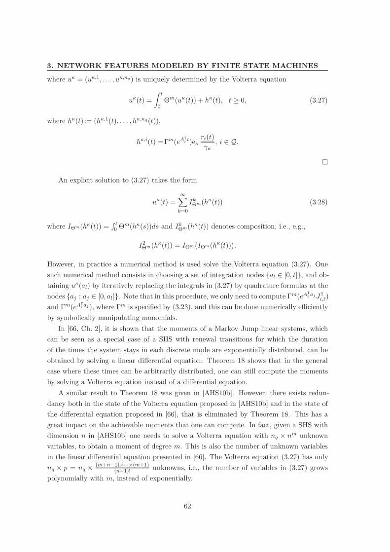
3. NETWORK FEATURES MODELED BY FINITE STATE MACHINES
where u& = (u&,1, . . . , u&,nq) is uniquely determined by the Volterra equation
u&(t) =) t
0#m(u&(t)) + h&(t), t " 0, (3.27)
where h&(t) := (h&,1(t), . . . , h&,nq (t)),
h&,i(t) =(m(eA!i t)e&
ri(t).&
, i + Q.
"
An explicit solution to (3.27) takes the form
u&(t) =%*
k=0Ik
!m(h&(t)) (3.28)
where I!m(h&(t)) =" t
0 #m(h&(s))ds and Ik!m(h&(t)) denotes composition, i.e., e.g.,
I2!m(h&(t)) = I!m
'I!m(h&(t))
(.
However, in practice a numerical method is used solve the Volterra equation (3.27). Onesuch numerical method consists in choosing a set of integration nodes {al + [0, t]}, and ob-taining u&(al) by iteratively replacing the integrals in (3.27) by quadrature formulas at thenodes {aj : aj + [0, al]}. Note that in this procedure, we only need to compute (m(eA!
i aj J!i,')
and (m(eA!i aj ), where (m is specified by (3.23), and this can be done numerically e"ciently
by symbolically manipulating monomials.In [66, Ch. 2], it is shown that the moments of a Markov Jump linear systems, which
can be seen as a special case of a SHS with renewal transitions for which the durationof the times the system stays in each discrete mode are exponentially distributed, can beobtained by solving a linear di!erential equation. Theorem 18 shows that in the generalcase where these times can be arbitrarily distributed, one can still compute the momentsby solving a Volterra equation instead of a di!erential equation.
A similar result to Theorem 18 was given in [AHS10b]. However, there exists redun-dancy both in the state of the Volterra equation proposed in [AHS10b] and in the state ofthe di!erential equation proposed in [66], that is eliminated by Theorem 18. This has agreat impact on the achievable moments that one can compute. In fact, given a SHS withdimension n in [AHS10b] one needs to solve a Volterra equation with nq # nm unknownvariables, to obtain a moment of degree m. This is also the number of unknown variablesin the linear di!erential equation presented in [66]. The Volterra equation (3.27) has onlynq # p = nq # (m+n!1)#···#(m+1)
(n!1)! unknowns, i.e., the number of variables in (3.27) growspolynomially with m, instead of exponentially.
62
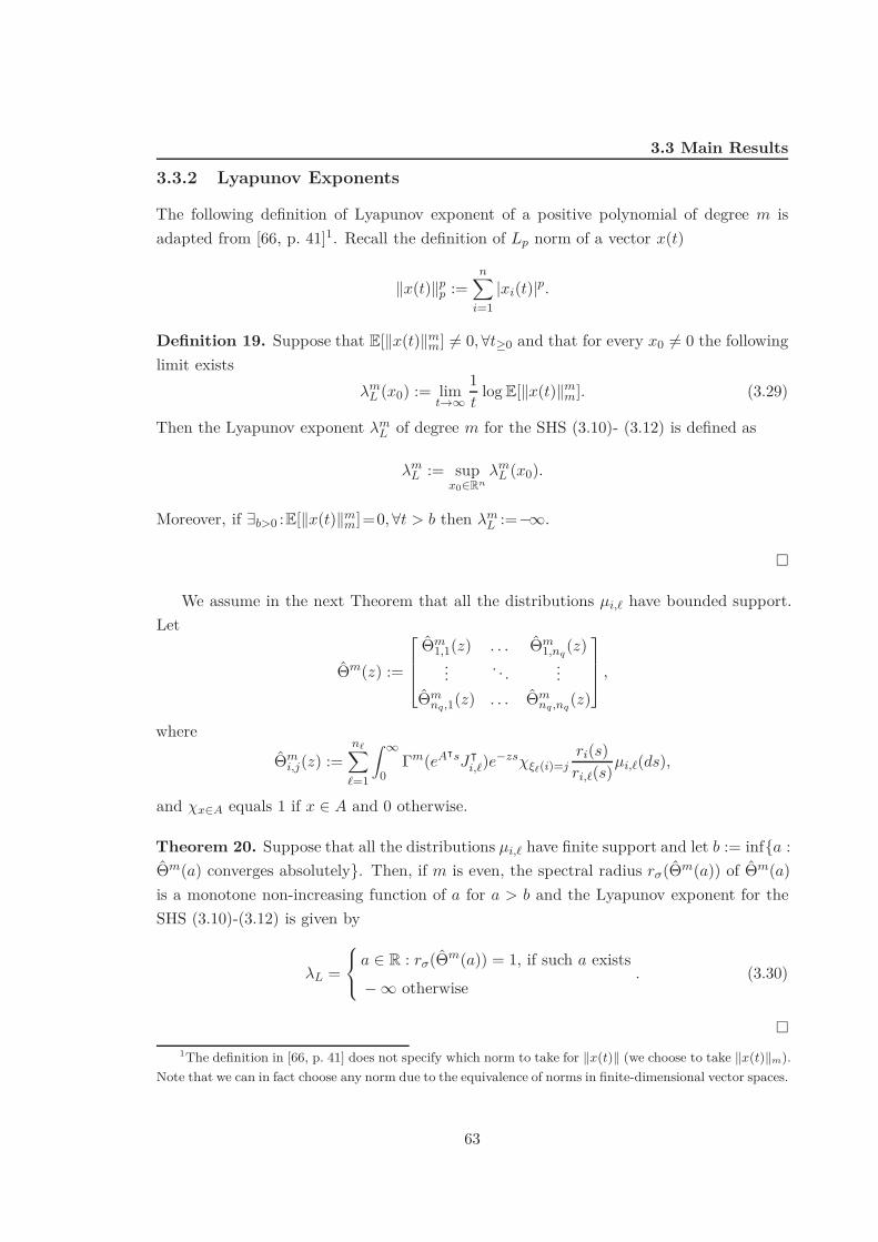
3.3 Main Results
3.3.2 Lyapunov Exponents
The following definition of Lyapunov exponent of a positive polynomial of degree m isadapted from [66, p. 41]1. Recall the definition of Lp norm of a vector x(t)
)x(t))pp :=
n*
i=1|xi(t)|p.
Definition 19. Suppose that E[)x(t))mm] 1= 0, 2t$0 and that for every x0 1= 0 the following
limit exists"m
L (x0) := limt'%
1t
logE[)x(t))mm]. (3.29)
Then the Lyapunov exponent "mL of degree m for the SHS (3.10)- (3.12) is defined as
"mL := sup
x0&Rn"m
L (x0).
Moreover, if 3b>0 :E[)x(t))mm]=0, 2t > b then "m
L :=0/.
"
We assume in the next Theorem that all the distributions µi,' have bounded support.Let
#m(z) :=
0
112
#m1,1(z) . . . #m
1,nq(z)
... . . . ...#m
nq,1(z) . . . #mnq,nq
(z)
3
445 ,
where
#mi,j(z) :=
n!*
'=1
) %
0(m(eA!sJ!
i,')e!zs/(!(i)=jri(s)ri,'(s)µi,'(ds),
and /x&A equals 1 if x + A and 0 otherwise.
Theorem 20. Suppose that all the distributions µi,' have finite support and let b := inf{a :#m(a) converges absolutely}. Then, if m is even, the spectral radius r"(#m(a)) of #m(a)is a monotone non-increasing function of a for a > b and the Lyapunov exponent for theSHS (3.10)-(3.12) is given by
"L =
+,
-a + R : r"(#m(a)) = 1, if such a exists0 / otherwise
. (3.30)
"1The definition in [66, p. 41] does not specify which norm to take for !x(t)! (we choose to take !x(t)!m).
Note that we can in fact choose any norm due to the equivalence of norms in finite-dimensional vector spaces.
63

3. NETWORK FEATURES MODELED BY FINITE STATE MACHINES
As we show next, Theorem 20 allows to establish necessary and su"cient stabilityconditions for the SHS with renewal transitions, which is defined in terms of a sum ofsecond moments. We say the SHS with renewal transitions is mean exponentially stable ifthere exists constants c > 0 and $ > 0 such that for every (x0, q0),
E[x(t)!x(t)] ! ce!!tx!0x0, 2t$0,
Corollary 21. Suppose that all the distributions µi,' have bounded support. Then the SHSwith renewal transitions is mean exponentially stable if and only if
r"(#2(0)) < 1. (3.31)
"Using the results in Chapter (2), once can show that mean exponential stability can
also be tested by asserting the feasibility of a set of linear matrix inequalities and by a testin terms of the Nyquist Criterion.
3.3.3 Probability Density Function
Let µ be the probability density function of the state of the SHS at time t, i.e.,"
E µ(ds) :=Prob[x(t) + E . Rn]. In this subsection we address the problem of obtaining informationon µ, based on its moments (3.19). It is well known that in the case where all the momentsare known, the measure µ can be uniquely determined [54], while in the case where onlya finite number of moments are known, this reconstruction is naturally not unique. Inthis latter case, an elegant procedure to obtain an explicit expression for an approximatingdistribution to µ, is the following (cf. [54]). Assume, for simplicity, that µ has boundedsupport, which without loss of generality (by proper scaling) can be assumed to be con-tained in the interval D := [0, 1]n = [0, 1] # · · · # [0, 1] (see [54] for the case of unboundedsupport). Given a continuous function f : D ,- R define the higher dimensional Bernsteinpolynomials as:
Br(f)(x) =*
k:0*ki*ri
f(k1r1
, . . . ,kn
rn)Pr,k(x)
where r = (r1, . . . , rn) is a vector of integers, and Pr,k(x) := 'ni=1
'riki
(xki
i (1 0 xi)ri!ki . It isshown in [54] that Br(f)(x) converges uniformly to f(x) as ri - /, 21*i*n. Thus, if welet Ir,k :=
"D Pr,k(x)µ(ds), we have that
*
0*ki*ri
f(k1r1
, . . . ,kn
rn)Ir,k (3.32)
is an approximation to E[f(x)] ="
E f(s)µ(ds) that converges to E[f(x)] as ri - /, 21*ri*n,and it is shown in [54] that a measure µr defined by
*
0*ki*ri
Ir,k(([k1r1
, . . . ,kn
rn]).
64

3.3 Main Results
is a discrete measure approximating µ in the sense that"
D f(s)µr(ds) -"
D f(s)µ(ds), forevery continuous function f : D ,- R, as ri - /, 21*i*n,where ((x) denotes the Diracmeasure located on x.
It is important to mention that the problem of recovering a probability density functionfrom its moments is regarded as a numerically ill-conditioned problem, meaning that smallerrors in the knowledge of the moments can produce large errors in the approximationfor the probability density function. In the procedure just described, one can see thatIr,n may have large errors for small error in the knowledge of the moments because ofthe large coe"cients that arise from writing Pr,n(x) as a sum of monomials. Thus, it isespecially important to have a computationally e"cient method to compute the moments,as provided by Theorem 18, so that one can obtain a good numerical precision in thisprocedure of obtaining an approximating distribution.
One way to interpret the procedure just described is that each integral Ir,n approximatesthe probability that x lies in a small neighborhood of (k1
r1, . . . , kr
rn). Instead of obtaining an
approximation one can use similar ideas to obtain an upper bound on the probability thatx belongs to a given region. That is, suppose, for example, that we wish to determine abound on the probability that a random variable y = g(x) is greater than a given value.Assume that y takes values in a compact set, which, without loss of generality, is assumedto be [0, 1]. Then we can choose a polinomial pn : [0, 1] - R$0 such that pn(x) " /[a,1],
a < 1, and obtain the following bound
Prob[y " a] ! E[pn(x)] (3.33)
where the right-hand side of (3.33) can be computed using Theorem 18. Note that whenpn(x) = x
a and pn(x) = x2
a2 , (3.33) correspond to the Markov and Chebychev inequalities,respectively.
Alternative approaches to estimate the probability density function of the state of theSHS include those based on the Focker-Plank equation and Dynkin’s formula. The Focker-Plank equation to the SHS with renewal transitions can be obtained by specializing theexpressions provided in [45], [41, Sec. 5.3], to this class of systems, and can be shown tobe a integro-partial di!erential equation. Besides the numerical di"culty and computationburden associated with solving this equation, the derivation of these Focker-Plank equationsrequires the map Jx to be invertible. The approach based on the Dynkin’s formula can befound in [25, Ch.3, Sec. 32.2] where a numerical method is provided to compute the expectedvalue of a given function E[f(x)], and a fortiori estimating the probability density functionfrom the relation E[/E(x)] = Prob[x + E]. Note that the approximation (3.32), whichcan be obtained with the methods derived in the present chapter, provides an alternativeto the method in [25, Ch.3, Sec. 32.2] to approximate the expected value of continuousfunctions of the state. Although we omit the derivations here, it is possible to prove
65

3. NETWORK FEATURES MODELED BY FINITE STATE MACHINES
that when specialized to SHSs with renewal transitions and to the case where f is amonomial, the recursive method provided in [25, Ch.3, Sec. 32.2] is equivalent to providingan approximation to (3.26) at each iteration 0 of the recursive algorithm, taking the form,
p*
l=1x[l]
0 v&,q0l (t), (3.34)
withv&(t) =
)*
k=0Ik
!m(h&(t)). (3.35)
This last equation converges to (3.28), and hence (3.34) converges to (3.26), but this it isclearly an ine"cient method to obtain the solution to the Volterra equation (3.27), whencompared to the method described in Subsection 3.3.1 (cf. [64]). Thus, by exploiting linear-ity and the special structure of the SHS with renewal transitions, our approach providesan insight that allows to compute moments more e"ciently, than when seeing the SHSwith renewal transitions as a piecewise deterministic process and specializing the approachproposed in [25, Ch.3, Sec. 32.2].
3.4 Numerical Examples
3.4.1 Round-robin protocols and packet drops - Batch Reactor
We consider here a numerical example of the round-robin scenario, considered in Subsec-tion 3.1.1. This example considers a linearized model of an open loop unstable batchreactor, described by (3.1), where
AP =
0
111112
1.38 00.2077 6.715 05.67600.5814 04.29 0 0.675
1.067 4.273 06.654 5.8930.048 4.273 1.343 02.104
3
444445,
BP =
0
111112
0 05.679 01.136 03.1461.136 0
3
444445, CP =
#1 0 1 010 1 0 0
$
.
(3.36)
We assume that only the outputs are sent through the network, using a round-robinprotocol. The system is controller by a PI controller, described by (3.2), where
AC =#
0 00 0
$, BC =
#0 11 0
$, CC =
#02 00 8
$, DC =
#0 025 0
$. (3.37)
This example appeared in [44]. To compare our results with the ones in [44] we consideruniformly and exponentially (µ([0, x)) = 1 0 exp(0"expx)) distributed time intervals hk.
66

3.4 Numerical Examples
This scenario can be modeled by a stochastic hybrid system with two discrete modesnq = 2, and using the description given in Subsection 3.1.1, where transitions are definedin an obvious way. The results are summarized in Table 3.1, where one can see thatour stability conditions eliminate the conservativeness of the stability conditions providedin [44].
Table 3.1: Stability conditions for the Batch Reactor Example
Nec. & Suf. Cond. Results taken from [44]no drops p = 0.5 no drops p = 0.5
Maximum support *
of Uniform Distribution0.112 0.0385 0.0517 0.0199
Max. expected value 1/$exp
of Exponential Distribution0.0417 0.0188 0.0217 0.00924
3.4.2 Delays - Inverted Pendulum
We consider here a numerical example for the scenario considered in Subsection 3.1.2where we illustrate the applicability of the results we present for stochastic hybrid systems.Suppose that the plant (3.6) is described by
AP =#0 11 0
$
, BP =#01
$
,
which by properly scaling the state and input can be viewed as a linearized model of a damp-free inverted pendulum. Moreover, suppose that the measure µs is uniform with supporton the interval [0, ! ], and fix Ts = 0.1s. A continuous-time state feedback controller issynthesized using LQR and is given by u(t) = KCx(t), KC = 0
%1 +
92 1 +
92&
, whichis the solution to the problem minu(t)
" %0 [xP (t)!xP (t)+u(t)2]dt, yielding "i(AP +BP KC) =
{01, 09
2}. We wish to investigate the stability and performance of the closed-loop wheninstead of the ideal networked-free case we consider the scenarios of Cases I and II. To thise!ect we define the quantity
e(t) = xP (t)!xP (t) + u(t)2,
which can be written as e(t) = x!Px, where in the network-free case P = I2 + K!CKC ,
and x = xP ; in case I, P = I3 and x = (xP , u); and in case II, P = diag(I2, 1, 0), andx = (xP , u, v). Note that, in the network-free case, e(t) is the quantity whose integral isminimized by LQR control synthesis and e(t) decreases exponentially fast at a rate $ = 2,since the dominant closed-loop eigenvalue equals "i(AP + BP KC) = 01. Note also that incases I and II, E[e(t)] converging to zero is equivalent to MSS, which is equivalent to SS andMES since the reset-time measures have finite support (! and !s are finite). Corollary 21
67
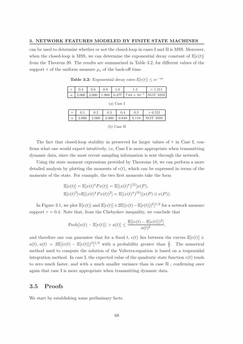
3. NETWORK FEATURES MODELED BY FINITE STATE MACHINES
can be used to determine whether or not the closed-loop in cases I and II is MSS. Moreover,when the closed-loop is MSS, we can determine the exponential decay constant of E[e(t)]from the Theorem 20. The results are summarized in Table 3.2, for di!erent values of thesupport ! of the uniform measure µs of the back-o! time.
Table 3.2: Exponential decay rates E[e(t)] ! ce!!t
! 0.4 0.6 0.8 1.0 1.2 > 1.211" 2.000 2.000 1.969 0.477 7.63 " 10!5 NOT MSS
(a) Case I
! 0.1 0.2 0.3 0.4 0.5 > 0.521" 2.000 2.000 2.000 0.849 0.118 NOT MSS
(b) Case II
The fact that closed-loop stability in preserved for larger values of ! in Case I, con-firms what one would expect intuitively, i.e, Case I is more appropriate when transmittingdynamic data, since the most recent sampling information is sent through the network.
Using the state moment expressions provided by Theorems 18, we can perform a moredetailed analysis by plotting the moments of e(t), which can be expressed in terms of themoments of the state. For example, the two first moments take the form
E[e(t)] = E[x(t)!Px(t)] = E[(x(t)!)(2)]'(P ),E[e(t)2]=E[(x(t)!Px(t))2] = E[(x(t)!)(4)]('(P ) $ '(P )).
In Figure 3.1, we plot E[e(t)] and E[e(t)]±2E[(e(t)0E[e(t)])2 ]1/2 for a network measuresupport ! = 0.4. Note that, from the Chebyshev inequality, we conclude that
Prob[|e(t) 0 E[e(t)]| > a(t)] ! E[(e(t) 0 E[e(t)])2]a(t)2 ,
and therefore one can guarantee that for a fixed t, e(t) lies between the curves E[e(t)] ±a(t), a(t) = 2E[(e(t) 0 E[e(t)])2]1/2 with a probability greater than 3
4 . The numericalmethod used to compute the solution of the Volterra-equation is based on a trapezoidalintegration method. In case I, the expected value of the quadratic state function e(t) tendsto zero much faster, and with a much smaller variance than in case II , confirming onceagain that case I is more appropriate when transmitting dynamic data.
3.5 Proofs
We start by establishing some preliminary facts.
68

3.5 Proofs
0 1 2 3 4 50
2
4
6
8
10
E[e(t)]E[e(t)]+2E[(e(t)−E[e(t)])2]1/2
E[e(t)]−2E[(e(t)−E[e(t)])2]1/2
(a) Case I
0 1 2 3 4 50
2
4
6
8
10
E[e(t)]E[e(t)]+2E[(e(t)−E[e(t)])2]1/2
max(E[e(t)]−2E[(e(t)−E[e(t)])2]1/2,0)
(b) Case II
Figure 3.1: Plot of E[e(t)], where e(t) is quadratically state dependent. For a fixed t, E[e(t)]lies between the dashed curves with probability > 3
4 .
First, let A(m), m > 0, denote the m-th fold Kronecker product of a matrix or a vectorA with itself, i.e.,
A(m) := A $ A · · · $ A6 78 9m
,
and recall that(A $ B)(C $ D) = (AC) $ (BD) (3.38)
(cf. [46]). Using (3.38), we can write (3.19) as
E[x1(t)i1x2(t)i2 . . . xn(t)in ] = E[(x(t)!)(m)c&], (3.39)
wherec& := e(i1)
1 $ · · · $ e(in)n , for -()) = [i1, . . . , in]. (3.40)
Second, let T (m, n) be the set of symmetric tensors, i.e., multilinear functions R onthe m-fold Rn # · · · # . . .Rn (cf. [85, Ch. 4]) such that
R(x1, x2, . . . , xm) = R(x"(1), x"(2), . . . , x"(m))
for every , : {1, 2, . . . , m} ,- {1, 2, . . . , m}, which is an one-to-one function, i.e., defines apermutation of indexes. We note that there is a natural identification between monomialsof degree m in Rn and T (m, n). In fact, to every m0degree monomial x[&] = xi1
1 xi22 . . . xin
n ,indexed by ), as in (3.21), we can associate an element b& of the following orthogonal basisof symmetric tensors
b& =*
j&J"
(e!j1) $ (e!j2) $ . . . $ (e!jm), 1 ! ) ! p (3.41)
where j belongs a set of .& permutations of indexes defined as follows
J& := {j = (j1, . . . , jm) : xj1xj2 . . . xjn = x[&], 2x&Rn} (3.42)
where ) : -()) = [i1, . . . , in]. Then one can obtain that
(x(t)(m))!c& = (x(t)(m))!d& (3.43)
69

3. NETWORK FEATURES MODELED BY FINITE STATE MACHINES
where d& := (b")!+"
. and we can write x(t)(m) in terms of the dual basis of b&, i.e.,
x(t)(m) =p*
&=1x[&](b&)! (3.44)
where p is given by (3.20). Let Ti(t) denote the transition matrix of the SHS starting atthe discrete mode q0 = i, i.e., x(t) = Tq0(t)x0 where
Ti(t) = eAq(t)(t!tr) . . . J(l0 (i),l1eA#l0 (i)Ji,l0eAit,
r = max{k + Z$0 : tk ! t}, and let
w&,i(t) := E[(Ti(t)))(m)d&], i + Q. (3.45)
We can express (3.19), or equivalently (3.39), in terms of w&,i(t), i + Q. In fact, us-ing (3.38), (3.39), and (3.43) we have that
E[(x(t)!)(m)c&] = E[(x(t)!)(m)d&]= (x!
0)(m)E[(Tq0(t)!)(m)d&]= (x!
0)(m)w&,q0(t).(3.46)
Third, note that for a matrix A + Rn#n, the map TA : Rp ,- Rp, y ,- v = TA(y) definedby
p*
&2=1v&2(b&2)! = A(m)
p*
&2=1y&2(b&2)!, (3.47)
can be simply described byv = (m(A)y (3.48)
where (m is given by (3.22). In fact, if A = [Aij ] = [(a1)! (a2)! . . . (an)!]!, then us-ing (3.38), the definition (3.42), and (3.44), we have that, for )1 : -()1) = [i1 i2, . . . in],
(Ax)[&1] = (a1)(i1) $ (a2)(i2) $ . . . $ (an)(in)x(m)
= 1.&1
*
j&J"1
aj1 $ aj2 $ . . . $ ajmx(m)
= 1.&1
*
j&J"1
aj1 $ aj2 $ . . . $ ajm
p*
&2=1(b&2)!x[&2]
=p*
&2=1B&1&2x[&2]
whereB&1&2 = 1
.&1
*
j&J"1
*
i&J"2
Aj1i1Aj2i2 . . . Ajnin . (3.49)
Applying the tensors b&1, 1 ! )1 ! p on both sides of (3.47) one also obtains that the linearmap (3.47) is described by (3.49) in the basis (bj)!, 1 ! j ! p.
70
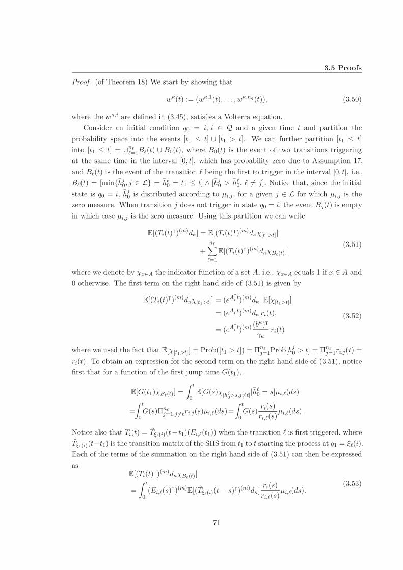
3.5 Proofs
Proof. (of Theorem 18) We start by showing that
w&(t) := (w&,1(t), . . . , w&,nq (t)), (3.50)
where the w&,i are defined in (3.45), satisfies a Volterra equation.Consider an initial condition q0 = i, i + Q and a given time t and partition the
probability space into the events [t1 ! t] : [t1 > t]. We can further partition [t1 ! t]into [t1 ! t] = :n!
'=1B'(t) : B0(t), where B0(t) is the event of two transitions triggeringat the same time in the interval [0, t], which has probability zero due to Assumption 17,and B'(t) is the event of the transition + being the first to trigger in the interval [0, t], i.e.,B'(t) = [min{hj
0, j + L} = h'0 = t1 ! t] ; [hj
0 > h'0, + 1= j]. Notice that, since the initial
state is q0 = i, hj0 is distributed according to µi,j, for a given j + L for which µi,j is the
zero measure. When transition j does not trigger in state q0 = i, the event Bj(t) is emptyin which case µi,j is the zero measure. Using this partition we can write
E[(Ti(t)!)(m)d&] = E[(Ti(t)!)(m)d&/[t1>t]]
+n!*
'=1E[(Ti(t)!)(m)d&/B!(t)]
(3.51)
where we denote by /x&A the indicator function of a set A, i.e., /x&A equals 1 if x + A and0 otherwise. The first term on the right hand side of (3.51) is given by
E[(Ti(t)!)(m)d&/[t1>t]] = (eA!i t)(m)d& E[/[t1>t]]
= (eA!i t)(m)d& ri(t),
= (eA!i t)(m) (b&)!
.&ri(t)
(3.52)
where we used the fact that E[/[t1>t]] = Prob([t1 > t]) = 'n!j=1Prob[hj
0 > t] = 'n!j=1ri,j(t) =
ri(t). To obtain an expression for the second term on the right hand side of (3.51), noticefirst that for a function of the first jump time G(t1),
E[G(t1)/B!(t)] =) t
0E[G(s)/[hj
0>s,j +=']|h'0 = s]µi,'(ds)
=) t
0G(s)'n!
j=1,j +='ri,j(s)µi,'(ds)=) t
0G(s) ri(s)
ri,'(s)µi,'(ds).
Notice also that Ti(t) = T(!(i)(t0 t1)(Ei,'(t1)) when the transition + is first triggered, whereT(!(i)(t0t1) is the transition matrix of the SHS from t1 to t starting the process at q1 = *'(i).Each of the terms of the summation on the right hand side of (3.51) can then be expressedas
E[(Ti(t)!)(m)d&/B!(t)]
=) t
0(Ei,'(s)!)(m)E[(T(!(i)(t 0 s)!)(m)d&] ri(s)
ri,'(s)µi,'(ds).(3.53)
71
3. NETWORK FEATURES MODELED BY FINITE STATE MACHINES
where Ei,'(s) := Ji,'eAs. By construction of the process E[(T(!(i)(t0s)!)(m)] = E[(T(!(i)(t0s)!)(m)] = w&,(!(i)(t0s). Replacing (3.52) and (3.53) in (3.51) and noticing that q0 = i + Qis arbitrary we obtain that
w&,i(t) = IiW (w&(t)) + (eA!
i t)(m) (b&)!.&
ri(t), i + Q. (3.54)
whereIW (w&(t)) :=
n!*
'=1
) t
0(Ei,'(!)!)(m)w&,(!(i)(t 0 !) ri(!)
ri,'(!)µi,'(d!)
An explicit solution to the set of equations (3.54) takes the form
w&(t) =%*
k=0Ik
W ((eA!i t)(m) (b&)!
.&ri(t)) (3.55)
where IkW denotes composition, and from (3.55) it is possible to conclude that w&,i(t)
belongs to the dual vector space of the symmetric tensors for every i + Q, and thereforecan be written as
w&,i(t) =p*
j=1u&,i
j (t)(bj)! (3.56)
Replacing (3.56) in (3.54) we getp*
j=1u&,i
j (t)(bj)! = (eA!i t)(m)(b&)! 1
.&ri(t)
+n!*
'=1
) t
0(Ei,'(!)!)(m)
p*
j=1u&,(!(i)
j (t 0 !)(bj)! ri(!)ri,'(!)µi,'(d!),
i + Q.
(3.57)
Applying the tensors bi, i + {1, . . . , n&} in (3.57), and using the fact that the maps (3.47)and (3.48) are equivalent, we obtain the set of equations (3.27).
Proof. (of Theorem 20)Similarly to (3.39) we can write
E[n*
j=1(xj(t))m] =
n*
j=1E[(x(t)!)(m)e(m)
j ], (3.58)
Each term of the summation E[(x(t)!)(m)e(m)j ] can be obtained from Theorem 18, where
the index ) in (3.26), (3.27), (18), should be taken as )j , given by
)j : -()j) =%j j . . . j
&, 1 ! j ! n.
72
3.5 Proofs
Due to the linearity of the Volterra equation we can obtainn*
j=1E[xj(t)p] =
p*
l=1x[l]
0 um,q0l (t), (3.59)
where um = (um,1, . . . , um,nq ) is uniquely determined by the Volterra equation
um(t) =) t
0#m(um(t)) + hm(t), t " 0, (3.60)
where hm(t) := (hm,1(t), . . . , hm,nq (t)),
hm,i(t) =(m(eA!i t)
n*
j=1e&j
ri(t)c
, i + Q.
It is then clear that the limit "L(x0) = limt'%1t log(E[)x(t))m
m]) exists for every x0 if andonly if the limit
"V := limt'%
1t
log()um(t))) (3.61)
exists, and "V = supx0 "L(x0) = "L. Note also that E[)x(t))mm] = 0, 2x0 , t > b > 0 if and
only if um(t) = 0, t > b > 0 in which case both "L and "V equal 0/ according to ourdefinitions.
Consider the setsU : {T + T (m, n) : T x(m) " 0}
andK : {x + Rp :
p*
i=1xib
i + U},
where bi is a basis for T (m, n) described by (3.41). The set K is a cone, i.e., K is a closedconvex set such that if y, z + K then $1y + $2z + K, for $1 " 0, $2 " 0 and is suchthat the set 0K := {0y : y + K} intersects K only at the zero vector. Moreover K is asolid cone, which in finite-dimensional spaces is equivalent to being reproducing, i.e., anyelement y + Rp can be written as y = y1 0 y2 where y1, y2 + K (cf. [56, p. 10]). In fact,let z + K be defined as !p
i=1 1ibi, where 1i = ( if i : -(i) = [i . . . i] and 1i = 0 otherwise.Then, from (3.41), z = (
!nj=1(ej)(j). Given any y + Rn, then y = y1 0 y2, for y1 = z + y
and y2 = z, which belong to K for su"ciently large (. Likewise one can also prove thatKnq := K # · · · # K 4 Rp # Rp # · · · # Rp, y = (y1, . . . , ynq ) + Knq if and only if yi + K,21*i*nq is a solid cone. We prove that the Volterra equation (3.60) has a positive kernelwith respect to the solid cone Knq , in the sense of Section 2.5, and therefore we can directlyapply Theorem 13 to conclude that, r"(#m(a)) is non-decreasing and that the root withlargest real part of det(I 0 #m(z)) is real and coincide with the unique value a such thatr"(#(a)m) = 1. As stated in Theorem 13, the zero a equals "V , given by (3.61), which inturn equal the Lyapunov exponent "L, provided this zero is not a removable singularity of
73
3. NETWORK FEATURES MODELED BY FINITE STATE MACHINES
a given complex function. The proof of this latter statement follows similar steps to theones provided in Theorem 4 and is therefore omitted.
To prove that the kernel of the Volterra equation (3.60) is a positive operator, we needto prove (cf. Section 2.5) that if y = (y1, . . . , ynq) + Knq then M(s)y + Knq , for every s > 0,where
M(s) :=
0
112
M1,1(s) . . . M1,nq(s)... . . . ...
Mnq,1(s) . . . Mnq,nq(s)
3
445 ,
andMi,j(s) :=
n!*
'=1(m(eA!sJ!
i,')/(!(i)=jri(s)ri,'(s) .
Note that if (z1, z2, . . . , znq ) = M(s)y then for a given s, each zi, 1 ! i ! nq can be writtenas a sum of terms taking the form (m(eA!sJ!
i,')yj multiplied by positive scalars. Thusto prove that zi + K and hence z + Knq , it su"ces to prove that w = (m(B)y + K foran arbitrary 1 ! j ! nq, y + K, and B + Rn#n. To this e!ect, using the fact that themaps (3.47) and (3.48) are equivalent, we have that
w :p*
i=1wi(bi)! = B(m)
p*
i=1yi(bi)!
belongs to K because !pi=1 wi(bi) belongs to U since
p*
i=1wi(bi)x(m) =
p*
i=1yi(bi)(B!)(m)x(m)
=p*
i=1yi(bi)(B!x)(m) " 0
where in the last equality we used the fact that !pi=1 yi(bi) + U .
3.6 Further Comments and References
As surveyed in [76], various models of SHSs [47], [38], [25] have been proposed di!ering onwhich of these features randomness come into play. See also [45], [41], [44], [66].
The class of SHS with renewal transitions can be viewed as a special case of the SHSmodel in [45], which in turn is a special case of a piecewise deterministic process [25], andalso a special case of a State-Dependent Jump-Di!usion [41, Sec. 5.3]. Stochastic Hybridsystems with renewal transitions can also be viewed as a generalization of a Markov JumpLinear System [66], in which the lengths of times that the system stays in each modefollow an exponential distribution, or as a generalization of an Impulsive Renewal System,in which there is only one discrete mode and one reset map.
74

4
Asynchronous Renewal Networks
In this chapter we consider networked control systems in which sensors, actuators, andcontroller transmit through asynchronous communication links, each introducing indepen-dent and identically distributed intervals between transmissions. We model these scenariosthrough impulsive systems with several reset maps triggered by independent renewal pro-cesses, i.e., the intervals between jumps associated with a given reset map are identicallydistributed and independent of the other jump intervals.
We provide stability results for impulsive systems triggered by superposed renewalprocesses, from which one can directly infer stability properties for the networked controlsystems just described. Our main result establishes that when the dynamic map a and thereset maps j' are linear, mean exponential stability is equivalent to the spectral radius of anintegral operator being less than one, which can be e"ciently tested numerically. To provethis result, we first derive conditions for mean exponential stability for impulsive systemswith general non-linear dynamic and reset maps. When specialized to linear dynamicand reset maps, these stability conditions can be expressed in terms of the existence ofa solution to an integro-di!erential equation, which, in turn, is related to the spectralradius of an integral operator. For the general nonlinear case, we show that the originof the impulsive system is (locally) stable with probability one if the linearization of theimpulsive system about zero equilibrium is mean exponentially stable, which justifies theimportance of studying the linear case.
To illustrate the applicability of our results, we consider the linearized model of a batch-reactor that we considered in the previous chapter, where we assumed that the sensorstransmit in a round-robin fashion through a single shared link. We can now test meanexponential stability in the case where the sensors transmit through two asynchronous linksboth introducing independent and identically distributed intervals between transmissions.
The remainder of the chapter is organized as follows. The connection between impulsivesystems triggered by superposed renewal processes and networked control systems is given
75

4. ASYNCHRONOUS RENEWAL NETWORKS
in Section 4.1. In Section 4.2 we formally defined an impulsive systems triggered by super-posed renewal processes. In Section 4.3 we state and discuss our main results. An exampleis given in Section 4.4. Our main result concerning stability of linear impulsive systems,is proved in Section 4.5, whereas the proofs of auxiliary results are given in Section 4.6.Further comments and references are provided in Section 4.7.
4.1 Modeling Networked Control Systems with ImpulsiveSystems
Consider a continuous-time plant and a controller described by
Plant: xP = fP (xP , u), y = g(xP ) (4.1)Controller: xC =fC(xC , y), u = h(xC , y). (4.2)
The controller is assumed to yield the closed-loop stable when the plant and the controllerare directly connected, i.e., u(t) = u(t), y(t) = y(t). However, sensors, actuators, and con-troller may be spatially distributed and linked via communication networks, in which casethis ideal assumption is not valid. Suppose that there are ny sensors, among which, ny arelinked to the controller via ny communication networks, i.e., each sensor transmits througha di!erent network. Then we can partition y as y = (yD, yD) := (gD(xP ), gD(xP )) = g(xP )where
yD = (y1, . . . , yny),
comprises the measurement signals yi + Rsi , 1 ! i ! ny of the ny sensors linked to thecontroller via a network, and yD comprises the measurement signals of the sensors whoseconnection to the controller is ideal. Therefore, partitioning y as y = (y1, . . . , yny , yD),yi + Rsi, we have yD(t) = yD(t). Likewise, assuming that there are nu actuators, amongwhich, nu communicate to the plant via a communication network, we can partition u asu = (uD, uD) := (hD(xC), hD(xC)) = h(xC), where
uD = (u1, . . . , unu),
comprises the actuation signals uj + Rrj , 1 ! j ! nu of the nu actuators linked to thecontroller via a network, and uD comprises the actuation signals of the actuators whoseconnection to the controller is ideal. Also here, partitioning u as u = (u1, . . . , unu , uD),uj + Rrj , we have uD(t) = uD(t). Let n' := ny + nu, and for a given + + {1, . . . , ny},let {t'
k, k " 0} denote the transmission times of the sensor y' and for a given + + {ny +1, . . . , n'}, let {t'
k, k " 0} denote the transmission times of the actuator u'!ny . Betweentransmission times we assume that yi and uj remain constant
y'(t) = y'(t'k), t + [t'
k, t'k+1), 1 ! + ! ny, (4.3)
76
4.2 Impulsive Systems Triggered by Superposed Renewal Processes
andu'!ny(t) = u'!ny(t'
k), t + [t'k, t'
k+1), 1 ! + 0 ny ! nu, (4.4)
while at transmission times we have the following update equations
y'(t'k) = y'(t'!
k ), 1 ! + ! ny, (4.5)
andu'!ny(t'
k) = u'!ny(t'!k ), 1 ! + 0 ny ! nu. (4.6)
We assume that in each of the n' networks that connect sensors and actuators to thecontroller, the intervals between transmissions are independent and identically distributed,i.e., {h'
k := t'k+1 0 t'
k} are independent and identically distributed random variables, andalso independent of the transmission intervals in the remaining networks. Defining,
e := (ey, eu) := (yD 0 yD, uD 0 uD), (4.7)
and using the fact that we can write y ='ey+gD(xP ), gD(xP )
(, we can model the networked
control system (4.1)-(4.7) as an impulsive system taking the form
x(t) = a(x(t)), t " 0, t 1= t'k, x(0) = x0,
x(t'k) = j'(x(t'!
k )), k " 1, + + L := {1, . . . , n'},
where x = (xP , xC , e) is the state;
a(x) =#fP
'xP , (eu + hD(xC , y), hD(xC , y))
(
fC'
xC , (ey + gD(xP ), gD(xP ))(
$
(4.8)
models the plant, controller, and error dynamics; and
j'(x) = (xP , xC , j'(e1), . . . , j'(en!)), (4.9)
models the transmissions at which the error associated with the transmitting sensor/actuatoris reset to zero, i.e., j'(ei) = 0, if i = +, and j'(ei) = ei, if i 1= +. The model (4.8) is termedin the next section an impulsive system triggered by superposed renewal processes.
4.2 Impulsive Systems Triggered by Superposed RenewalProcesses
Impulsive systems triggered by superposed renewal processes are defined as follows
x(t) = a(x(t)), t " 0, t 1= t'k, x(0) = x0,
x(t'k) = j'(x(t'!
k )), k " 1, + + L := {1, . . . , n'},(4.10)
77

4. ASYNCHRONOUS RENEWAL NETWORKS
where the duration of the intervals {h'k = t'
k+1 0 t'k, k " 0} between jumps times tk
associated with a given reset map j', are independent and identically distributed and alsoindependent of the jump intervals {hj
k, j 1= +, j + L}. In (4.10), the notation x(t'!k )
indicates the limit from the left of x at the point t'k.
The maps a and j', + + L are assumed to be di!erentiable and globally Lipschitz andthe origin is an equilibrium point, i.e., a(0) = 0 and j'(0) = 0, 2'&L. We denote by n
the dimension of the state x + Rn. We assume that the intervals between jump times{h'
k = t'k+1 0 t'
k, + + L}, are described by a probability density function f'(t) " 0, withfinite support in the interval [0, .'], .' > 0. We assume that the f'(t) are di!erentiable1
on (0, .') and we denote the survivor function by
r'(s) := Prob[h'k > s] =
) +!
sf'(r)dr, k " 1, s + [0, .'],
and the hazard rates by"'(!') := f'(!')
r'(!'), !' + B'. (4.11)
The system (4.10) is initialized at t = 0, where it is subsumed that a time !' := 0t'0
has elapsed since the last jump associated with map +. In other words, we consider thatfor each reset map + + L, the first jump times t'
1, satisfy
Prob([t'1 > s]) = r'(!' + s)
r'(!'), s + [0, .' 0 !'], (4.12)
which is the probability that the next jump after t = 0 occurs after time s, given that att = 0 a time !' has elapsed since the map j was triggered.
We need to define the following auxiliary process
v(t) = (v1(t), . . . , vn!(t)), v'(t) := t 0 t'k!
, v(0) = !, (4.13)
where k' := max{k " 0 : t'k ! t}. The process v(t) keeps track of the time elapsed
since the last jump associated with each of the reset maps, and therefore at time t = 0,v(0) = ! = (!1, . . . , !n!) = 0(t1
0, . . . , tn!0 ). Note that v(t) + B, where
B := B1 # · · · # Bn! . (4.14)
and B' := [0, .'], + + L. We also define
x(t) := (x(t), v(t)), x(0) := x = (x0, !), (4.15)
which, as we shall see, is a Markov process, although, in general, x(t) is not. In fact, (4.15)can be constructed as a piecewise deterministic process (cf. Theorem 35 in Section 4.6).
We consider the following definition of stability for (4.10).1We assume di!erentiability on most functions of interest in the chapter to avoid complicating the
proofs of our main results.
78
4.3 Main Results
Definition 22. We say that (4.10) is mean exponentially stable (MES) if there existsconstants c > 0, $ > 0 such that for any initial condition x0, the following holds
E[x(t)!x(t)] ! ce!!tx!0x0, 2t$0. (4.16)
"
4.3 Main Results
We start by providing in Subsection 4.3.1 a stability result for (4.10) with general non-linear dynamic and reset maps. Building upon this result, we are able to establish ourmain result, presented in Subsection 4.3.2, which provides necessary and su"cient stabilityconditions when the dynamic and reset maps in (4.10) are linear. In Subsection 4.3.3 werelate the stability of the non-linear impulsive system with that of its linearization.
4.3.1 Non-linear Dynamic and Reset Maps
We start by providing an important auxiliary results, which results from that fact that (4.15)can be constructed as a piecewise deterministic process (cf. Theorem 35 in Section 4.6).
Theorem 23. If V is a di!erentiable function, such that
E[*
t!k*n
|V (x(t'k)) 0 V (x(t'!
k ))|] < /, 2n&N (4.17)
where + + L, then
E[V (x(t))]=V (x)+E) t
0AV (x(s))ds, 2t$0, (4.18)
whereAV (x) := 2
2!V (x)+
XxV (x) +n!*
'=1"'(!')[V ((j'(x), 30
' (!))) 0 V (x)],(4.19)
for x = (x, !) + Rn # B, and XxV (x) :=!ni=1
,V (x),xi
ai(x).
"
The following result establishes general conditions for (4.10) to be MES, providinga stochastic analog of a well-known result for deterministic non-linear systems (cf. [53,Th.4.10]). The proof can be found in the Section 4.6.
79
4. ASYNCHRONOUS RENEWAL NETWORKS
Theorem 24. The system (4.10) is MES if and only if there exists a di!erentiable positivefunction V (x) which equals zero at zero, and positive constants c1, c2, r such that for everyx = (x, !) + Rn # B,
c1)x)2 ! V (x) ! c2)x)2 (4.20)AV (x) ! 0r)x)2 (4.21)
"
4.3.2 Linear Dynamic and Reset Maps
In this subsection, we consider the following linear version of (4.10)
x(t) = Ax(t), t " 0, t 1= t'k, x(0) = x0,
x(t'k) = J'x(t'!
k ), k " 1, + + L,(4.22)
where {h'k = t'
k+1 0 t'k, k " 1} and t'
0 are as described for (4.10).Define a variable ! = (!1, . . . , !n!) + B where !j + Bj . Furthermore, let Bj =
B1 # . . . Bj!1 # Bj+1 # · · · # Bn! and define the two following maps: 3' that removesthe component + from the vector ! , i.e., 3' : B ,- B', 3'(!) = (!1, . . . , !'!1, !'+1, . . . , !n!);and 30
' that sets the component + of the vector ! to zero, i.e.,
30' : B ,- B, 30
' (!) = (!1, . . . , !'!1, 0, !'+1, . . . , !n!). (4.23)
Let Pa be the Cartesian product space of n' real symmetric matrix functions, eachdefined in B', i.e., if P = (P1(!1), . . . , Pn!(!n!)) + Pa, then P'(!')! = P'(!'), 2!l + B'. Sumand multiplication by scalar in Pa are defined in a natural way and we consider the usualinner product 'Q, R( = !n!
'=1"
B!Q'(!')!R'(!')d!' for Q, R + P. Then we define the space
P 4 Pa as the space of elements P 4 Pa such that 'P, P ( < /, which can be shown to bea Hilbert space. Let L : P ,- P be the following integral operator
(Q1, . . . , Qn!) = L(P1, . . . , Pn!) (4.24)
where Q'(3'(!)) := R(30' (!)),
R(!) :=n!*
"=1
) #
0(J"e
As)!P"(3"(!)+s1n!!1)J"eAs r"(!, s)
r"(!)f"(!" + s)
r"(!")ds,
(4.25)
r'(!, s) := 'n!j=1,j +='rj(!j + s), r'(!) := 'n!
j=1,j +='rj(!j), . := min{.' 0 !', + + L} and 1n!!1is a vector with n' 0 1 components set to one.
For example for n' = 1, (4.24), (4.25) take the form
Q1 =) +1
0(J1eAs)!P1J1eAsf1(s)ds, (4.26)
80
4.3 Main Results
where P1 and Q1 are symmetric matrices, and in this special case P is a finite dimensionalspace since its elements are matrices and not matrix-valued functions. For n' = 2, we have
Q1(!2) =) #1
0(J1eAs)!P1(!2 + s)J1eAs r2(!2 + s)
r2(!2) f1(s)ds
+) #1
0(J2eAs)!P2(s)J2eAsr1(s)f2(!2 + s)
r2(!2) ds,
!2 + [0, .2],
Q2(!1) =) #2
0(J2eAs)!P2(!1 + s)J2eAs r1(!1 + s)
r1(!1) f2(s)ds
+) #2
0(J1eAs)!P1(s)J1eAsr2(s)f1(!1 + s)
r1(!1) ds.
!1 + [0, .1],
(4.27)
where .1 = min(.1, .2 0 !2), and .2 = min(.1 0 !1, .2).Since L operates in a real space P, to define its spectral radius we consider the com-
plexification of P (cf. [56, p. 77]), i.e., the space P := {Q = P + iR : P, R + P}. ForQ = P + iR + P , one defines L(Q) := L(P ) + iL(R). The spectral radius is defined asfollows:
r"(L) := max{|"| : " + ,(L)}, (4.28)
where ,(L) := {" : L 0 "I is not invertible in P} denotes the spectrum and I the identity.Note that, defining P as a real space, and defining the spectral radius of L acting on P asin (4.28) is generally di!erent from considering P to be a complex space, where the matrixcomponents P' of P = (P1, . . . , Pn!) + P are self-adjoint matrices, and defining the spectralradius of L as usual. We shall use the first construction since this will allow us to readilyuse the results for positive operators given in [56] to prove our results in Section 4.5.
The following is the main result of the chapter.
Theorem 25. The system (4.22) is MES if and only if r"(L) < 1.
"
The theorem is proved in Section 4.5. We discuss next how one can numerical computer"(L), and some special cases of the impulsive system, for which one can provide alternativestability conditions to Theorem (25).
Computation of the Spectral Radius of L
One can show that L is a compact operator (using, e.g., [14, p. 165, Th. 4.1]) and thereforeits spectrum consists either of a finite set of eigenvalues " : LP = "P for some P + P ora countable set of eigenvalues with no accumulation point other than zero (cf., e.g., [14,p. 117, Th. 2.34]). For simplicity, consider first the case n' = 2, where L is describedby (4.27). A numerical method to compute r"(L) is the following. Take a grid of points in
81

4. ASYNCHRONOUS RENEWAL NETWORKS
the interval !1j + [0, .1], 1 ! j ! nd1, and !2j + [0, .2], 1 ! j ! nd2 and consider the mapobtained by replacing P (!1), P (!2) in (4.27) by interpolating piecewise polynomials at thepoints {P1(!2k), P2(!1k)}, and evaluating the integrals (4.27) at the grid points to obtain{Q1(!2k), Q2(!1k)}. This yields a finite rank operator, from the chosen space of piecewisepolynomials in P, to itself, and assuming nd1 = nd2 = nd, its matrix representation hasdimension 2n2
dn(n + 1)/2, since Pi, Qi, i + {2} are symmetric. Denote by Lnd , the finiterank operator obtained. The method just described is known as the collocation method, aspecial case of the projection method (cf. [14, p. 177]), and one can conclude from the resultsin [14] that r"(Lnd) - r"(L) as nd - /, for typical piecewise polynomial approximations,such as the trapezoidal approximation.1 For general n', this method involves computingthe spectral radius of a nn!
d n'n(n + 1)/2 matrix, which means that computing r"(L) mayrequire significant computational e!ort when the number of reset maps is large.
Special Cases
A first special case is when there is only one reset map, i.e., n' = 1. In this case P issimply the finite dimensional space of symmetric matrices and L is the linear map P1 ,- Q1between two finite dimensional space defined in (4.26). In this case r"(L) < 1 reduces totesting if the spectral radius of a matrix is less than one. This condition can be shownto be equivalent to the stability condition given in [AHS11d], where the case n' = 1 isanalyzed using a di!erent approach, based on Volterra equations, which does not appearto generalize to the problem considered in this chapter.
A second special case is when the maps A, J' commute, i.e., AJ' = J'A, and J'Jr =JrJ', 2',r&L. In this case, the following result, proved in the Section 4.6, provides alternativestability conditions to Theorem 25.
Theorem 26. When the maps A and J', + + L commute, the system (4.22) is MES if
2" +n!*
'=1$' < 0, (4.29)
where " is the maximum real part of the eigenvalues of A and the $' are given by
$'=
+:,
:-
0 / , if r"(J!' $ J!
' ) = 0
a + R :) +!
0e!asf'(s)ds = 1
r"(J!' $ J!
' ) , otherwise(4.30)
"1 In fact, from the spectral characterization of compact operators described above, one can conclude
from [14, p.232, Th. 5.5 and p.250, Example 5.14]), that the eigenvalues of the compact operators Lnd
converge to the eigenvalues of the compact operator L which allows us to conclude that r$(Lnd ) # r$(L).
82

4.3 Main Results
It is important to emphasize, that even for the commuting case , the condition (4.29)is su"cient but not necessary, as shown in the following example.
Example 27. Suppose that A = [0]2#2, n' = 1, J1 =#a1 00 0
$
, and J2 =#0 00 a2
$
, where
a1 > 1, a2 > 1. Then, " = 0 and, from (4.30), we can conclude that $1 > 0 and $2 > 0.Thus (4.29) does not hold. However, since the state remains constant between jump timest'k, + + {1, 2}, and component i is reset to zero when the reset map i is triggered, i + {1, 2},
we conclude that E[x(t)!x(t)] = 0, t > max(.1, .2) and therefore (4.22) is MES.
"
A third special case is when the probability densities f' correspond to exponentialdistributions, i.e., r'(y) = e!-!y. Since the support of the probability density functions isnot bounded we assume the following
2" <n!*
'=11', (4.31)
where " is the maximum real part of the eigenvalues of A. This assumption can be shownto assure that the expected value of a quadratic function of the state of the system doesnot go unbounded between jump times. This assertion can be obtained using a similarreasoning to [AHS11d, Th. 3]. The next theorem states that, in this case, we can providestability conditions in the form of LMIs. The result is proved in Section 4.6.
Theorem 28. Suppose that r'(y) = e!-!y and that (4.31) holds. Then the system (4.22)is MES if and only if
3P >0 : A!P + PA +n!*
'=11'(J!
' PJ' 0 P ) < 0 (4.32)
"
4.3.3 Stability with Probability One
The following definition is adapted from [60].
Definition 29. We say that the origin of the system (4.10) is (locally) stable with probabilityone if for every - > 0 and % > 0 there is a ((-, %) > 0 such that, if )x0) < ((-, %) then
Prob{ sup%>t$0
)x(t)) " %} ! -. (4.33)
The following result shows that one can assert stability with probability one of theorigin of (4.10), by establishing mean exponential stability for its linearization, which canbe tested by Theorem 25. The proof is provided in Section 4.6.
83

4. ASYNCHRONOUS RENEWAL NETWORKS
Theorem 30. If (4.22) is MES with A = ,,xa(x)|x=0 and J' = ,
,xj'(x)|x=0, + + L where a
and j' are the non-linear maps in (4.10), then the origin of (4.10) is stable with probabilityone.
"
This theorem allow us to conclude a property analogous to the one proved in [62]stating that a standard periodic sampled-data connection of a non-linear plant and a non-linear controller is locally stable if the sampled-data connection of the linearization of theplant and of the linearization of the controller is stable. In fact, from Theorem 30, we canconclude that in the setup of Section 4.1, the non-linear networked control system describedby (4.8), (4.9) is stable with probability one, if the networked control system obtained byreplacing fP , g, fC , and h, by their local linearizations about the zero equilibrium is meanexponentially stable, which can be tested by Theorem 25.
4.4 Example - Batch Reactor
This example considers the control of a linearized model of an open loop unstable two-input two-output batch reactor, controlled by a PI controller. The plant and controllertake the form (4.1), and (4.2), with fP (xP , u) = AP xP + BP u, g(xP ) = CP xP , andfC(xC , y) = ACxC + BC y, h(xC , y) = CCxC + DC y. The expressions for (AP , BP , CP )and (AC , BC , CC , DC) are given in (3.36) and (3.37). The actuator is directly connectu(t) = u(t). However, the sensors are linked to the plant through communications networks.
In Section 3.4.1, it is assumed that the outputs are sent in a round-robin fashion througha single shared communication network. When the distribution of the intervals betweenconsecutive transmissions is assumed to be, e.g., uniform with a support ., we can use theresults in Chapter 3 to study the stability of this system.
Suppose now that, instead of transmitting the two measurements in a round robin fash-ion through the same communication network, the two sensors transmit data through twoindependent communication links. We assume that both links are shared with other usersand that the intervals between consecutive transmissions can be modeled by independentprocesses with support in the interval [0, .'] for the link associated with the output y',l + {1, 2}. We can cast this system in the framework os Section 4.1, and use the techniquesdeveloped here to study the stability in this latter case.
When two links are used to transmit the measurements of the two sensors, we can useTheorem 25 to investigate the stability of the system as a function of the distributionsfor the intersampling times on each network. The results obtained are summarized inFigure 4.1 for the case of uniform distributions with di!erent supports.
84

4.5 Proof of Theorem 25
00.02 0.06 0.1 0.14 0.18 0.22 0.260
0.02
0.06
0.1
0.14
0.18
0.22
0.26
0.3
T2(ms)
T 1(ms)
o−MES .−Not MES
Figure 4.1: MES for various values of the support of a uniform distributions of the transmis-sion intervals of two independent links.
For the case of two independent links we take a grid of values of .1 and .2, i.e., thesupport of the distributions between transmissions, and test mean exponential stability ofthe closed-loop using the numerical method described in Section 4.3 to compute the spectralradius of the operator defined in the Theorem 25. The results obtained are summarized inthe Figure 4.1. If the distributions of the two links have the same support then stabilityis preserved for every .1, .2 + [0, .], with . = 0.18. It is interesting to compare this withthe case of a round-robin single-link protocol where it was shown in Section 3.4.1 thatthe maximum support of a uniform distribution for which stability could be guaranteedwas . = 0.11. With a round-robin protocol, this would lead to a distribution betweenconsecutive samples for the same sensor that is triangular with support 0.22. However,note that in this case the duration of the intervals between transmissions of the two outputsare not independent, and a di!erent approach must be used to assert stability. If thetwo links have di!erent supports one can conclude from the Figure 4.1 that the meanexponential stability of the closed-loop is lost for a lower value of the support of thedistributions associated with the output y2 than the value of the support associated withthe output y1.
4.5 Proof of Theorem 25
We prove the Theorem 25 through three steps: (i) we show that specializing the stabilityconditions of Theorem 24 to the system (4.22), yields mean square stability conditionsfor (4.22) in terms of the existence of a solution to an integro-di!erential equation; (ii) weestablish that these conditions are equivalent to the existence of a solution to a Fredholmequation; (iii) we prove that (ii) is equivalent to the spectral radius of the integral operatorof the Fredholm equation being less than one.
85

4. ASYNCHRONOUS RENEWAL NETWORKS
(i) MES for Linear Impulsive Systems
The Theorem 24 can be specialized to (4.22) as follows.
Theorem 31. The system (4.22) is MES if and only if for every di!erentiable functionsY (!) and Z(!) such that a1I < Y (!) < a2I, 2*&B and b1I < Z(!) < b2I, ,*&B there existsa di!erentiable function X(!), such that c1I < X(!) < c2I, 2*&B, and for every ! + B,
n!*
'=1
2
2!'X(!) + A!X(!) + X(!)A+
n!*
'=1"'(!')[J!
' X(30' (!))J' 0 X(!) + Z(!)] + Y (!) = 0,
(4.34)
where 30' is defined by (4.23), and ai, bi, ci, i + {1, 2} are positive constants.
"
Proof. To prove su"ciency we use Theorem 24 and consider the function V (x(t)) =x!(t)X(v(t))x(t) where x = (x(t), v(t)) and X(!), ! + B satisfies (4.34) and the remainingconditions of the theorem. Then from (4.19) we have that
A(x!X(v)x) = x![n!*
'=1
2
2!'X(v) + A!X(v) + X(v)A+
+n!*
'=1"'(v')[J!
' X(30' (v))J' 0 X(v)]]x
(4.35)
Using (4.34) we obtain
A(x!X(v)x)=0x![(n!*
'=1"'(v')Z(v) + Y (v))]x!0a1)x)2,
and since c1I ! X(v) ! c2I, we have that c1)x)2 ! V (x) ! c2)x)2. Using Theorem 24,applied to (4.22), we conclude that (4.22) is MES.
Necessity follows by using the same arguments as in the proof of Theorem 24 andnoticing that the function (4.69) takes the form V (x) = x!
0X(!)x0, for x = (x0, !) + Rn #B,
X(!) = X1(!) + X2(!), (4.36)
where
X1(!) =) +%
0E* [%(t)!Y (v(t))%(t)]dt, (4.37)
X2(!) =*
k>0,'&LE* [%(t'
k)!Z(v(t'k))%(t'
k)],
86

4.5 Proof of Theorem 25
%(t) is the transition matrix of the system (4.22), i.e.,
%(t) = eA(t!t!rr )J'r!1 . . . J'1eAh
!11 J'0eAh
!00 , (4.38)
where {+j + L, j " 0} is the triggered sequence of reset maps, r = max{k : tk ! t} andE* emphasizes that expectation subsumes that the process %(t) depends on the initialconditions ! of the process v(t). Since from Theorem 24, c1)x0)2 ! V (x) ! c2)x0)2 itfollows that c1I ! X(!) ! c2I. From [25, p.92, Th.(32.2)]) it follows that
A(x!0X1(!)x0) = 0x!
0Y (!)x0
and from [25, p.90,91] we have that
E[x!0X2(!)x0] = E[
) %
0"T (v(t))x(t)!Z(v(t))x(t)],
where"T (!) :=
n!*
j=1"j(!j), (4.39)
from which one can conclude again from [25, p.92, Th. (32.2)] that
A(x!0X2(!)x0) = 0"T (!)x!
0Z(!)x0.
Thus, for every (x0, !), we have
A(x!0X(!)x0) = 0x!
0(Y (!) + "T (!)Z(!))x0 (4.40)
Computing A(x!X(v)x) from (4.19) we obtain (4.35) which must be equal to (4.40) whenx = (x0, !) is replaced by x = (x, v), from which we conclude (4.34).
(ii) Fredholm Equation (25)
Let U be the space of elements (U1(!1), . . . , Un!(!n!)) + P for which U'(!') " 0, 2'&L, 2*!&B! .The space V 4 U is defined similarly but requiring U'(!') > 0, 2'&L, 2*!&B! .
Theorem 32. The system (4.10) is MES if and only if for every di!erentiable functionsY (!) and Z(!) such that a1I < Y (!) < a2I, 2*&B and b1I < Z(!) < b2I, ,*&B , there existsa solution P + V to the Fredholm equation
P = L(P ) + U, (4.41)
where U =(U1,. . ., Un!),U'(3'(!)):=W (30
' (!)), (4.42)
87

4. ASYNCHRONOUS RENEWAL NETWORKS
andW (!) :=
n!*
'=1
) +
0eA!sZ(! + s1n!)eAs r'(!, s)
r'(!)f'(!' + s)
r'(!')ds+
) +
0eA!sY (! + s1n!)eAs'n!
'=1r'(!' + s)
r'(!')ds
.
"
Proof. Suppose that (4.10) is MES and therefore there exists a solution X to (4.34) givenby (4.36). Let
P (3'(!)) := X(30' (!)), 3'(!) + B'. (4.43)
We prove next that X(!) satisfies
X(!)=W (!)+n!*
'=1
) +!
0(J'e
As)!X(30' (! +s1n!))J'e
As r'(!, s)r'(!)
f'(!' + s)r'(!')
ds.(4.44)
Then su"ciency follows by directly using (4.44) in (4.43), and noticing that the fact thatX(!), given by (4.36), satisfies X(!) > c1I, 2*&B, implies that P + V.
To this e!ect, we start by conditioning the integrand in (4.37) on the time of the firstjump t1 := min{t'
1, + + L},
E* [%(t)!Y (v(t))%(t)] = E* [(%(t)!Y (v(t))%(t))1[t1>t]]
+n!*
'=1E* [(%(t)!Y (v(t))%(t))1C!(t)]
(4.45)
where C'(t) = [min{tj1, j + L} = t'
1 = t1 ! t] ; [tj1 > t1, j 1= +], is the event that jump + is
the first to trigger, given that a trigger has occurred at time t. Using (4.12) the first termon the right hand side of (4.45) is given by eA!tY (! + t1n!)eAt'n!
'=1r!(*!+t)
r!(*!) . Note that fora function G(t1),
E* [G(t1)1C!(t)] =) t
0E[G(s)1[tj
1>s,j +=']|t'1 = s]f'(!' + s)
r'(!')ds
=) t
0G(s) r'(!, s)
r'(!)f'(!' + s)
r'(!')ds
and that %(t) = %'(t 0 t1)(J'eAt1) when the transition + + L is first triggered, where%'(t 0 t1) is the transition matrix from t1 to t starting the process at 30
' (! + s1n!) where30
' is defined by (4.23). Thus
E* [%(t)!Y (v(t))%(t)1C!(t)] =) t
0(J'e
As)! . . .
E.0! (*+s1n! )[%(t0s)!Y (v(t 0 s))%(t0s)]J'e
As$'(!, s)ds,(4.46)
88
4.5 Proof of Theorem 25
where $'(!, s) := r!(*,s)r!(*)
f!(*!+s)r!(*!) . By construction of the process
E.0! (*+s1n! )[(%'(t0s)!Y (v(t 0 s))%'(t0s)]=
E.0! (*+s1n! )[%(t0s)!Y (v(t 0 s))%(t0s)].
(4.47)
Replacing (4.47) in (4.46) and (4.46) and (4.45) we obtain
X1(!)=n!*
'=1X'
1(!) +) +
0eA!tY (! + t1n!)eAt'n!
'=1r'(!' + t)
r'(!')dt (4.48)
whereX'
1(!)=) %
0
) t
0E.0
! (*+s1n! )[(J'eAs)!(%(t0s)!Y (v(t 0 s)) . . .
%(t0s)(J'eAs)$(!, s)]dsdt
Changing the order of integration in this last expression we have that (4.48) can be writtenas
X1(!) =) +
0eA!tY (! + s1n!)eAt'n!
'=1r'(!' + t)
r'(!')dt+
n!*
'=1
) +
0(J'e
As)!X1(30' (! +s1n!))J'e
Asr'(!,s)r'(!')
f'(!'+s)r'(!')
ds
With similar computations one can conclude that
X2(!)=n!*
'=1
) +
0eA!sZ(! + s1n!)eAs r'(!, s)
r'(!)fl(!' + s)
r'(!')ds+
n!*
'=1
) +
0(J'e
As)!X2(30' (! +s1n!))J'e
Asr'(!,s)r'(!)
f'(!'+s)r'(!')
ds
Since X(!) = X1(!) + X2(!) adding X1(!) and X2(!) we obtain (4.44).Conversely, suppose that there exists a solution P + V to (4.41). Then one can verify
thatX(!)=W (!)+
n!*
'=1
) +!
0(J'e
As)!P'(3'(!)+s1n!!1)J'eAs r'(!, s)
r'(!)f'(!' + s)
r'(!')ds
(4.49)
satisfies all the assumptions of the function X(!) of Theorem 31, and therefore (4.10) isMES. In fact, if there exists a solution P + V to (4.41) one can obtain an explicit expressionfor the solution to (4.41) (cf. Theorem 33), which is given by
P =%*
i=0Li(U), (4.50)
where Li denotes the composite operator obtained by applying i times L, e.g., L2(P ) =L(L(P )) and L0(P ) := P . From (4.50) we can conclude that P is bounded and di!eren-tiable with respect to ! , since we assume that the f' are di!erentiable. Then, it is clear
89
4. ASYNCHRONOUS RENEWAL NETWORKS
that X(!) is bounded, X(!) " W (!) > c1I, 2*&B , for some c1 > 0 and (4.34) can beobtained by direct computation.
(iii) Positive Solution of the Fredholm Equation
As a prelude to the next result, we note that U is a cone in the Hilbert space (and henceBanach space, with the usual norm inherit by the inner product) P, in the sense of [56]since (i) it is closed; (ii) if U, W + U then $1U + $2W + U for $1 " 0 and $2 " 0; and(iii) the set1 0U := {0P : P + U} intersects U only at the zero vector. Moreover, thiscone is reproducing in P, i.e., if Z + P, then there exists U, W + U such that Z = U 0 W
(take for example, Ui(!) = Zi(!) + %I and Wi(!) = %I for su"ciently large % > 0 such thatPi(!) + %I > 0 for all i + {1, . . . , n'}, ! + B). The operator L is a positive operator withrespect to U , i.e., L(U) + U if U + U .
Theorem 33. The equation (4.41) has a solution P + V if and only if r"(L) < 1.
"
Note that the main result, Theorem 25, can be concluded from Theorems 32, 33.
Proof. Su"ciency follows from the fact that if r"(L) < 1 then P = !%i=0 L
i(U) exists whichis the solution to P = L(P ) + U . Since L is a positive operator with respect to U , P is asummation of U + V plus elements in U . Thus, taking into account the definitions of Uand V, we conclude that P belongs to V.
To prove necessity, we start by noticing that it is possible to prove that the dualcone (cf. [11, Sec. 2.6]2) of U can be identified with itself, i.e., using the nomenclatureof [11, Sec. 2.6], U is self-dual. The proof follows similar arguments used to prove thatthe cone of positive semi-definite matrices is self-dual (cf. [11, p.52]), and is thereforeomitted. From [56, p.22, Th. 2.5], we conclude that the adjoint operator L" is also apositive operator with respect to U , and using [56, Th. 9.2] which states that a completelycontinuous positive operator with respect to a reproducing cone has an eigenvalue thatequals the spectral radius and an eigenvector that belongs to the solid cone, we concludethat there exists W + U (other than the zero element) such that
L"(W ) = r"(L")W. (4.51)1Recall that addition and multiplications by scalar are defined in a natural way in P , e.g. if P =
(P1, . . . , Pn! ) $ P then %P := (%P1, . . . , %Pn! )}2The nomenclature used in [56, Ch. 2] is adjoint cone instead of dual cone
90

4.6 Proofs of Auxiliary Results
In fact, L" is a compact operator, since L is a compact operator (cf. [2, p.178]), whichcan be concluded from [14, p. 165, Th. 4.1], and a compact operator in a Banach space iscompletely continuous (cf. [2, p.177]). Suppose that r"(L) " 1 and (4.41) has a solutionP + V. Then r"(L") = r"(L) " 1. Taking the inner product on both sides of (4.41) withW + U , such that (4.51) holds, yields
'W, P ( = 'W,L(P )( + 'W, U( 6
'W, P ( = 'L"(W ), P ( + 'W, U( 6
'W, P ( (1 0 r"(L")) = 'W, U( (4.52)
Now 'W, P ( " 0, since W, P + U . Moreover, one can conclude that 'W, U( > 0, since W isdi!erent from the zero element in U and one can conclude from (4.42) that U + V. Thus,from (4.52) we conclude that r"(L") = r"(L) " 1 leads to a contradiction.
4.6 Proofs of Auxiliary Results
Proof of Theorems 23) and 24
We start by describing a construction for the process x, described by (4.15), which mim-ics the construction of a piecewise deterministic process, as described in [25, p. 59]. Let) := {u1
k, u2k, k " 0} where {u1
k} and {u2k} are mutually independent and identically dis-
tributed random variables uniformly distributed in the interval [0, 1]. Let also 4x(s, x(tk)),4v(s, v(tk)) be the flows at time s of the systems described by x(t) = a(x(t)) and v(t) = 1with initial condition x(tk) and v(tk), respectively. Note that 4v(s, v(tk)) = v(tk) + s1n! .Set k = 0 and t0 = 0, x(t0) = (x0, !), and consider the process x(t) = (x(t), v(t)) obtainedby iteratively repeating:
(I) Obtain hk from
hk = inf{t : e!" t
0 $T (/v(s,v(tk)))ds ! u1k}. (4.53)
where "T is described by (4.39). Set tk+1 = tk + hk, and for t + [tk, tk+1) make
x(t) ='4x(t 0 tk, x(tk)), 4v(t 0 tk, v(tk))
((4.54)
(II) Make x(tk+1) = 5(u2k, x(t!
k+1)), where
5(w, (x, !) )=(j'(x), 30' (!))/
w&(!!!1
j=1%j(&j)%T (&) ,
!!
j=1%j (&j)%T (&) ]
, (4.55)
91
4. ASYNCHRONOUS RENEWAL NETWORKS
and /x&A denotes the characteristic function, i.e.,
/w&A =
+,
-1 if w + A
0, if w /+ A. (4.56)
"
Remark 34. Note that (4.53) simply states that
Prob[hk > s|x(tk)] = 'n!j=1rj(s + vj(tk)), 2k$0
and (4.55) simply states that
Prob[x(tk) = (j'(x(t!k )), 30
' (v(t!k )))|x(t!
k )] = "'(!j(t!k ))
"T (!(t!k )) .
We choose to use the description (I) and (II) to mimic the piecewise deterministic processconstruction in [25, p. 59], which allows us to use the results from [25].
"
The next Theorem establishes the connection between (4.10), (4.13), and piecewisedeterministic processes.
Theorem 35. The stochastic process (x(t), v(t)), described by (4.10) and (4.13), can berealized in the probability space ) and constructed as the piecewise deterministic processdefined by the steps (I) and (II).
"
Proof. For the process (x(t), v(t)), described by (4.10), (4.13), define {tk " 0} with tk <
tk+1, 2k$0 as a set containing the union of all the jump times in (4.10), i.e., {tk " 0} =:n!
'=1{t'r!
, r' " 0}, let {hk := tk+1 0 tk, k " 0}, h!1 := 0, and consider the following discrete-time process
zk := (hk!1, x(tk), v(tk)). (4.57)
There exist a one to one relation between zk and x(t), described by (4.10), and (4.13). Infact, given a sample path (x(t), v(t)) one can identify the jump times tk by the times atwhich v'(tk) = 0 for some +, and from these construct hk and hence zk. Conversely, fromzk we can obtain hk and hence tk, and construct (x(t), !(t)) from (x(tk), (v(tk)) as
(x(t), v(t)) = (4x(t 0 tk, x(tk)), 4v(t 0 tk, v(tk))),tk ! t < tk+1.
(4.58)
92

4.6 Proofs of Auxiliary Results
Moreover, zk is a discrete-time Markov process. To see this, it su"ces to prove that
Prob(zk+1 +D|zr, 0 ! r ! k)=Prob(zk+1 +D|zk), 2k$0, (4.59)
where D is a measurable set. Since at tk, a time !'(tk) has elapsed since the last jumpassociated with the reset map + + L, the time tk+1 equals tk+1 = tk + hk, where
hk := min'&{1,...,n!}
{w'k},
and w'k are random variables such that Prob(w'
k > s) = r!(v!(tk)+s)r!(v!(tk)) . Thus,
Prob(hk+1 > s|zr, 0 ! r ! k) = 'n!'=1
r'(v'(tk) + s)r'(v'(tk)) , (4.60)
Let *k+1 denote which reset map triggers at tk+1, i.e.,
*k+1 := argmin'&{1,...,n!}{w'k}.
Then,Prob[*k+1 = +|hk + [s, s + %) ; zr, 0 ! r ! k] =
Prob[hk + [s, s + %) ; *k+1 = +|zr, 0 ! r ! k]!n!
j=1 Prob[hk + [s, s + %) ; *k+1 = j|zr, 0 ! r ! k]. (4.61)
Now,Prob[hk + [s, s + %) ; *k+1 = +|zr, 0 ! r ! k]= Prob[w'
k + [s, s + %) ; wjk > w'
k, 2j +='|zr, 0 ! r ! k]
=) s+#
s'n!
j=1,j +='
rj(vj(tk) + q)rj(vj(tk))
f'(v'(tk) + q)r'(v'(tk)) dq
(4.62)
Replacing (4.62) in (4.61), taking the limit as % - 0, and dividing the numerator anddenominator of the right hand side of (4.61) by 'n!
j=1rj(vj(tk + s)), we obtain
Prob[*k+1 = +|hk = s ; zr, 0 ! r ! k]
= "'(v'(tk) + s)"T (v(tk) + s1n!)
="'(v'(t!
k+1))"T (v(t!
k+1)).
where "T (v(t!k+1)) := !n!
'=1 "'(v'(t!k+1)). Thus, we conclude that
Prob[(x(tk),v(tk))=(j'(x(t!k )), 30
' (v(t!k )))|hk ;zr, 0!r!k]
= "'(v'(t!k ))
"T (v(t!k ))
(4.63)
From (4.63), and (4.60), we conclude that
Prob[hk +[c, d], x(tk+1)+Ex, v(tk+1)+Ev|zr, 0!r !k]
=n!*
'=1[) d
c/j!(/x(s,x(tk)))&Ex-/v(s,x(tk))&Ev . . .
('n!j=1,j +='
rj(vj(tk) + s)rj(vj(tk)) )f'(v'(tk) + s)
r'(v'(tk)) ]ds,
(4.64)
93
4. ASYNCHRONOUS RENEWAL NETWORKS
where /(... ) denotes the characteristic function (4.56). Note that (4.64) depends only onzk = (hk!1, x(tk), v(tk)) and thus the Markov property (4.59) holds.
Consider now the piecewise deterministic process defined by steps (I) and (II) and let
yk := (hk!1, x(tk), v(tk))
where h!1 = 0, and hk!1, tk, x(tk), v(tk) are now the variables defined in steps (I) and (II).Then, by construction of the process and Remark 45, we immediately obtain that (4.60),and (4.63), also hold for this process, and this implies that (4.64) also holds for thisprocess. Thus yk is a Markov process with the same transition probability function, i.e., analternative realization to zk. Since there is a one-to-one relation between zk and the processdefined by (4.10), (4.13), and there is a one-to-one relation between yk and the processdefined by the piecewise deterministic process construction described by steps (I) and (II),and both processes are completed in the same way between jump times (see (4.54), (4.58)),we conclude that the process (4.10), (4.13) can be constructed as the piecewise deterministicprocess specified by steps (I) and (II).
Proof. (of Theorem 23) Theorem 35 allows us to apply the results available in [25]. Inparticular, Theorem 23 follows directly from [25, p.33, (14.17)], [25, p.66, Th. (26.14)]and [25, p. 70, Rem. (26.16)]), provided that we can prove that the assumption in [25,p.60, (24.4)] that the expected value of the number of jumps up to a given time t isbounded, which when specialized to the stochastic process (x(t), v(t)), described by (4.10),is equivalent to saying that E[!n!
'=1 N'(t)] < /, where
N'(t) := max{k + N : t'k ! t}. (4.65)
This is in fact true, since each N'(t) is a renewal process [79] with intervals betweenrenewal times following a probability density function f' with no atom points, and thereforeE[N'(t)] < / (cf. [79, p. 186]).
Proof. (of Theorem 24) To prove su"ciency, we use Theorem 23 applied to the function
W (x(t), t) := er1tV (x)
where V (x) satisfies (4.20) and (4.21), r1 is a positive constant such that r1 > rc2
, and it isimplicit that the process (x(t), t) is a piecewise deterministic process if x(t) is a piecewise
94

4.6 Proofs of Auxiliary Results
deterministic process (cf. [25, p.84]). We need to show that W satisfies (4.17). Since weassume that a and j' are globally Lipschitz, we have )a(x)) ! L1)x), 2x&Rn and for every+ + L, we have )j'(x)) ! L2)x), 2x&Rn . Thus, between jump times,
)x(t))2 ! e2L1(t!t!k))x(tk))2, t + [t'
k, t'k+1),
(cf. [53, p.107, Exercise 3.17]) and at jump times, )x(t'k))2 ! (L2)2)x(t'!
k ))2. Thus,
E[)x(t))2] ! E[e2L1t'n!'=1(L2)2N!(t)])x0)2 (4.66)
where N'(t) is the number of jumps associated with the reset map + up to the time t,described by (4.65). We also have
E[*
t!k*n
|W (x(t'k)) 0 W (x(t'!
k ))|]
! E[*
t!k*n
c2er1n)x(t'k)))2]
! e2L1ner1n)x0)2n!*
j=1
%*
k=0c3(L2)2kE[/t!
k*n] (4.67)
where we used (4.20), and (4.66), and /(... ) denotes the characteristic function (4.56). Notethat E[/t!
k*n] = Prob[N'(n) " k]. The fact that the right-hand side of (4.67) is boundedis a direct application of [79, p.186, Th. 3.3.1], and therefore W satisfies (4.17).
From Theorem 23
E(W (x(t), t)) = W (x, 0) + E[) t
0AW (x(s), s)ds]
for an initial condition x = (x0, !). From [25, p. 84], we can conclude that
AW (x(s), s) = r1W (x(s), s) + er1sAV (x(s))
and using (4.21) we obtain
E(W (x(t), t)) ! W (x, 0)+
E[) t
0r1W (x(s), s) 0 rer1s)x(s))ds]
Using (4.20) and interchanging expectation with integral operations, we obtain
E(W (x(t), t)) ! W (x, 0) + (r1 0 r
c2)
) t
0E[W (x(s), s)]ds.
which implies, from the integral form of the Gronwall’s inequality [3, Lemma 1], that
E[V (x(t))er1t] = E[W (x(t), t)]! E[W (x, 0)]e(r1! r
c2)t = V (x)e(r1! r
c2)t
. (4.68)
95
4. ASYNCHRONOUS RENEWAL NETWORKS
Note that we can apply the Gronwall’s inequality since r1 0 rc2
> 0, and this is the reasonto work with W , instead of directly using V . From (4.68), we conclude that
E[V (x(t))] ! V (x)e! rc2
t
and using (4.20), we conclude that:
E[)x(t))2] ! 1c1E[V (x(t))] ! 1
c1V (x)e! r
c2t
! c2c1
)x0)2e! r
c2t.
Necessity is obtained by proving that
V (x) := V1(x) + V2(x) (4.69)
satisfies (4.20) and (4.21) where
V1(x) :=) +%
0Ex[x(s)!Y (v(s))x(s)]ds
V2(x) :=n!*
'=1
*
k>0Ex[x(t'!
k )!Z(v(t'!k ))x(t'!
k )]ds,
Ex emphasizes that expectation subsumes that the process starts at an initial conditionx = (x0, !), and a1I < Y (!) < a2I, 2! + B, and b1I < Z(!) < b2I, 2! + B, aredi!erentiable functions.
To see that V (x) " c1)x0)2 denote by t1 the time of the first jump, which can be fromany of the n' reset maps, and note that V (x) " a1
" t10 Ex[x(s)!x(s)]ds + b1Ex[x(t!
1 )!x(t!1 )]
for any t1 " 0. Let L1 be a Lipchitz constant for a, )a(x)) ! L1)x), which exists sincewe assume a is di!erentiable. Then we have x(t)!x(t) " x!
0x0e!2L1t, 2t$0 (cf. [53, p.107,Exercise 3.17]). Thus V (x) " c1x!
0x0 where c1 = a1" t1
0 e!2L1tdt + b1e!2L1t1 > 0, 2t1>0.To see that V (x) ! c2)x0)2, note that since (4.10) is MES, we have that Ex[x(t)!x(t)] !
a2ce!!tx!0x0 for some constant c > 0. Thus V1(x) ! a2 c
!x!0x0, and V2(x) ! k2x!
0x0 wherek2 := !n!
'=1!%
k=1 E[b2ce!!t!k ]. Note that E[e!!t!
k ] = 606k!1, where eta0 = E[e!!h!k ], 6 =
E[e!!h!k1 ] < 1, for some 1 ! k1 < k, and therefore k2 < /. Thus, V (x) ! c2)x0)2 where
c2 = a2c! + k2.
It follows from [25, p. 92, Cor. (32.6)]) that V1(x) is di!erentiable since, as requiredin [25, p. 92, Cor. (32.6)]) "T (!), is continuous. From [25, p.92, Th. (32.2)]
AV1(x) = 0x!0Y (!)x0
and from [25, p.90,91] we have that
E[V2(x)] = Ex[) %
0"T (v(t))x(t)!Z(v(t))x(t)dt],
96

4.6 Proofs of Auxiliary Results
from which one can conclude again from [25, p.92, Th. (32.2)] that
AV2(x) = 0"T (!)x!0Z(!)x0.
and that V2(x) is di!erentiable (again by [25, Cor.(32.6)]). Thus V (x) is di!erentiable andAV (x) ! 0rx!
0x0 for r = a1.
Proof of Theorems 26 and 28
Proof. (of the Theorem 26) From the explicit solution to (4.22), described by (4.38), andthe commuting property, we obtain that
E[x(t)!x(t)] = x!0eA!teAt'n!
'=1E[(J!' )N!(t)JN!(t)
' ]x0, (4.70)
where N'(t) is described by (4.65). From [AHS11d, Th. 4], we can conclude for somesymmetric matrix C and for $' described by (4.30), we have that E[(J!
' )N!(t)JN!(t)' ] ! Ce!!t,
if r"(J!' $ J!
' ) 1= 0. If r"(J!' $ J!
' ) = 0, the state is reset to zero after a finite number ofjumps, from which the result follows.
Proof. (of the Theorem 28) Due to the memoryless property of the exponential distributionit is ready to establish that in this special case, the stochastic process defined by (4.22)can be constructed as a stochastic hybrid system with renewal transitions in the senseof [AHS09b] with one discrete mode and n' reset maps characterized by matrices J' andprobability density functions f'. In [AHS09b] we provided necessary and su"cient stabilityconditions for the stability of stochastic hybrid systems with renewal transitions. Althoughwe restricted ourselves to the case where the transition probability density functions havebounded support, the results provided in [AHS09b] can be generalized to the case of un-bounded support using the same arguments provided in [AHS09b] for the special case wherethe stochastic hybrid system has only one discrete mode and only one reset map. Then,under the assumption (4.31), mean exponential stability can be shown to be equivalent to(special case of [AHS09b, Th.9.D])
2R>03P >0 :n!*
'=1Q'(P ) 0 P = 0R (4.71)
97
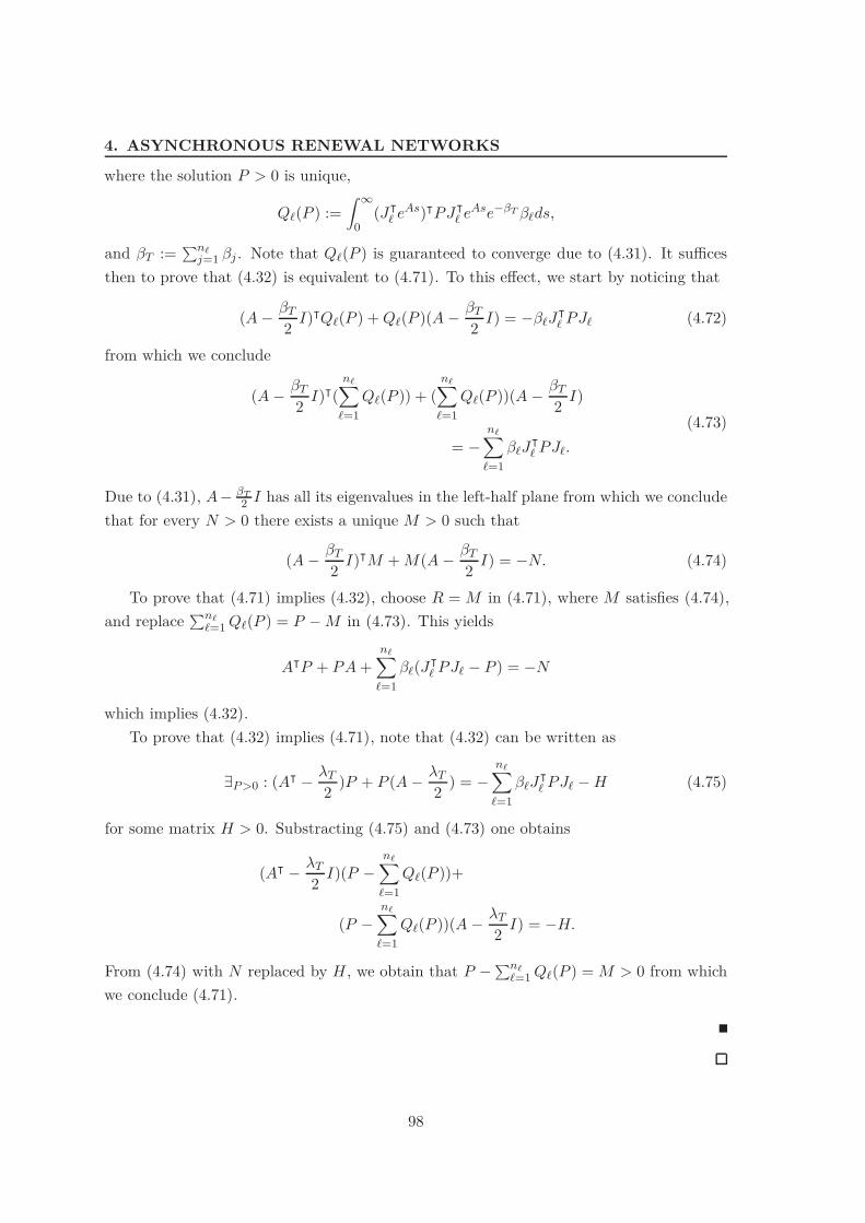
4. ASYNCHRONOUS RENEWAL NETWORKS
where the solution P > 0 is unique,
Q'(P ) :=) %
0(J!
' eAs)!PJ!' eAse!-T 1'ds,
and 1T := !n!j=1 1j . Note that Q'(P ) is guaranteed to converge due to (4.31). It su"ces
then to prove that (4.32) is equivalent to (4.71). To this e!ect, we start by noticing that
(A 0 1T
2 I)!Q'(P ) + Q'(P )(A 0 1T
2 I) = 01'J!' PJ' (4.72)
from which we conclude
(A 0 1T
2 I)!(n!*
'=1Q'(P )) + (
n!*
'=1Q'(P ))(A 0 1T
2 I)
= 0n!*
'=11'J
!' PJ'.
(4.73)
Due to (4.31), A 0 -T2 I has all its eigenvalues in the left-half plane from which we conclude
that for every N > 0 there exists a unique M > 0 such that
(A 0 1T
2 I)!M + M(A 0 1T
2 I) = 0N. (4.74)
To prove that (4.71) implies (4.32), choose R = M in (4.71), where M satisfies (4.74),and replace !n!
'=1 Q'(P ) = P 0 M in (4.73). This yields
A!P + PA +n!*
'=11'(J!
' PJ' 0 P ) = 0N
which implies (4.32).To prove that (4.32) implies (4.71), note that (4.32) can be written as
3P >0 : (A! 0 "T
2 )P + P (A 0 "T
2 ) = 0n!*
'=11'J
!' PJ' 0 H (4.75)
for some matrix H > 0. Substracting (4.75) and (4.73) one obtains
(A! 0 "T
2 I)(P 0n!*
'=1Q'(P ))+
(P 0n!*
'=1Q'(P ))(A 0 "T
2 I) = 0H.
From (4.74) with N replaced by H, we obtain that P 0!n!
'=1 Q'(P ) = M > 0 from whichwe conclude (4.71).
98

4.6 Proofs of Auxiliary Results
Proof of the Main Result
Proof. (of the Theorem 30) We rewrite the dynamic and reset maps in (4.10) as
a(x) = Ax + fe(x), j'(x) = J'x + ge'(x), (4.76)
where fe(x) := a(x) 0 Ax, and ge'(x) := j'(x) 0 J'x are di!erentiable functions such that
)fe(x)))x)
- 0, and )ge'(x)))x)
- 0, as )x) - 0 (4.77)
(cf. [53, p.138]). Let V (x(t)) = x(t)!X(v(t))x(t), where x(t) is described by (4.15) andX(!), ! + B satisfies (4.34) and c1I < X(!) < c2I, 2! + B. Then, there exists ' > 0 suchthat
AV (x) = 0r(x) ! 0d1)x)2, 2x:.x.*0 (4.78)
for some d1 > 0, where AV (x) is given by (4.19). This expression (4.78) can be obtainedby directly replacing (4.76) in (4.19), and using (4.77) in a similar fashion to the proof ofan analogous result for deterministic non-linear systems (cf. [53, p.139, Th. 4.7]).
Using similar arguments to [60, Th. 1,Ch. 2], we consider the stopped process xS(t) :=x(t ; !m), where t ; !m := min(t, !m); !m = inf{t : x(t) /+ Bm} is the first exit time fromthe set Bm := {x : V (x) < m}; and m ! 02
c1is such that Bm . {(x, !) : )x) ! '}] and
thus, from (4.78). It is easy to see that x(t ; !m) is a piecewise deterministic process andfrom (4.19) and (4.78),
AV (x(t ; !m)) =
+,
-0 r(x) if x + Bm
0 otherwise.(4.79)
Considering (4.18) for the process xS and using (4.79), we obtain that Ex[V (x(t ; !m))] !V (x), i.e., V (x(t;!m)) is a super-martingale. From this latter fact, and using the fact thatlimt'0 Ex[V (x(t))] = V (x), (cf. [25, p.77, Th. (27.6)]), we can apply the super-martingaletheorem [60, p.26, Eq. 7.4], and conclude that
Probx[ sup%>t$0
V (x(t ; !m)) " m] ! V (x)m
(4.80)
where Probx denotes probability with respect to the Markov process x started at initialcondition x = (x0, !). Given %, -, choose m = min(0,#)2
c1, and ( =
;1mc2
. Then, for any)x0) ! (,
Probx[ sup%>t$0
)x(t ; !m))) " %] !
Probx[ sup%>t$0
V (x(t ; !m)) " m]! V (x)m
! c2)x0)2
m!-
(4.81)
i.e., the origin of (4.10) is stable with probability one.
99
4. ASYNCHRONOUS RENEWAL NETWORKS
4.7 Further Comments and References
Several references to related work on networked control systems can be found in [43],including systems with asynchronous data transmissions, e.g., [97], and systems withindependent and identically distributed intervals between transmission, e.g, [69]. Seealso [44], [89], [AHS11d], [27]. However, the networked control problem we consider here,and the associated class of impulsive systems, seem to have not been studied in the litera-ture. Stability results for deterministic impulsive systems can be found in [77], [62]. Theproof of our results builds upon results for piecewise deterministic systems [25] and thestochastic Lyapunov approach [60].
100

5
Dynamic Protocols
In this chapter we address the problem of designing a protocol for network access in anetworked control system so that: (i) the range of parameters characterizing the networkedcontrol system that yield the networked control system stable is enhanced; (ii) optimalperformance is achieved with respect to a cost function which is quadratic with respect tothe states of the plant. As in the previous chapters, the network is assumed to introducestochastic intervals between transmissions, delays and packet drops. However, the way wemodel delays in this chapter di!ers from previous chapters.
We consider two frameworks for the problem: (i) an emulation framework, in whichonly the protocol is to be designed; and (ii) a direct design framework, in which both theprotocol and the controller are to be designed. In the emulation framework, we propose adynamic protocol specified as follows. Associated to each node there is a set of quadraticstate functions, which are evaluated at a given transmission time. The node allotted totransmit is the one corresponding to the least value of these quadratic state functions.These protocols are shown to be more general than quadratic protocols and MaximumError First-Try Once Discard protocols, considered in the literature. We establish twostability results for the networked control system, both providing conditions in terms oflinear matrix inequalities (LMIs) for investigating the stability in a mean exponential senseof given protocols, and conditions in terms of BMIs to design quadratic state functions,specifying the dynamic protocol, that yield the networked closed loop stable. The firststability result allows to prove that if the networked closed loop is stable for a staticprotocol then we can provide a dynamic protocol for which the networked closed loop isalso stable. This is the main result obtained in this framework and gives an analyticaljustification on why one should utilize dynamic protocols rather than static. The secondstability result allows for obtaining an observer-protocol pair that reconstructs the stateof an LTI plant in a mean exponential sense to the case where transmission intervals arestochastic. We illustrate through benchmark examples, that the conditions in this chapter
101
5. DYNAMIC PROTOCOLS
are significantly less conservative than other conditions that previously appeared in theliterature.
A drawback of the emulation framework is that full state knowledge is assumed forprotocol implementation, which restricts the range of applicability of these protocols. Con-sidering a direct design framework, we tackle the problem of simultaneously designing thescheduling sequence of transmissions and the control law so as to optimize a quadraticobjective. The plant is assumed to be disturbed by Gaussian noise, and for simplicity werestrict here the intervals between transmissions to be constant and consider no delaysand no packet drops. Using the framework of dynamic programming, we propose a rolloutstrategy by which the scheduling and control decisions are determined at each transmissiontime as the ones that lead to optimal performance over a given horizon assuming that fromthen on controller and sensors transmit in a periodic order and the control law is a standardoptimal law for periodic systems. We show that this rollout strategy results in a protocolwhere scheduling decisions are based on the state estimate and error covariance matrixof a Kalman estimator, and must be determined on-line. The resulting protocol obtainedfrom the rollout algorithm can be implemented in a distributed way both in wireless andwired networks, based on previous data sent from sensors and actuators, as opposed tothe requirements of the protocol obtained with the emulation framework where full-stateis generally required. It follows by construction of rollout algorithms that our proposedscheduling method can outperform any periodic scheduling of transmissions. We illustratethis fact with an example.
The remainder of the Chapter is organized as follows. In Section 5.1 we address theemulation problem. We address the problem formulation in Subsection 5.1.1, establishour main results in Subsection 5.1.2, and provide an illustrative example in 5.1.3. In Sec-tion 5.2 we address the direct design problem. In Subsection 5.2.1 we address the problemformulation, in Subsection 5.2.2 we establish our main results, and in Subsection 5.2.3 wegive an illustrative example. We provide the proof of the main results in Section 5.3 andwe give further comments and references in Section 5.4.
5.1 Emulation
5.1.1 Problem Formulation
We start by introducing the networked control stability problem and then we show that itcan be casted into analyzing the stability of an impulsive system.
102

5.1 Emulation
5.1.1.1 Networked Control Set-up
We consider a networked control system in which sensors, actuators, and a controller, areconnected through a communication network, possibly shared with other users. The plantand controller are described by the following state-space model:
Plant: xP = AP xP + BP u, y = CP xP (5.1)Controller: xC =ACxC + BC y, u = CCxC + DC y. (5.2)
Following an emulation approach, we assume that the controller has been designed tostabilize the closed loop, when the process and the controller are directly connected, i.e.,u(t) = u(t), y(t) = y(t), and we are interested in analyzing the e!ects of the network onthe stability of the closed loop. We denote the times at which a node transmits a messageby {tk, k + N}, and assume that, u and y are held constant, between transmission times,i.e.,
u(t) = u(tk), y(t) = y(tk), t + [tk, tk+1), k " 0. (5.3)
We denote by e the error signal between process output and controller input (y 0 y) andbetween controller output and process input (u 0 u). In particular,
e(t) := (eu(t), ey(t)) := (u(t) 0 u(t), y(t) 0 y(t)). (5.4)
We assume that while m nodes compete for the network, only one of them is allowed totransmit at each given transmission time. However, in our terminology a single transmittingnode could be associated with several entries of the process output y or with severalentries of the controller output u. For simplicity, we assume that the sensors and actuatorshave been ordered in such a way that we can partition the error vectors eu and ey aseu = (eu1, . . . , eunu), where each eui(t) + Rai is the error associated with an actuator nodei + {1, . . . , nu}, and ey = (ey1, . . . , eyny ), where each eyj(t) + Rbj is the error associatedwith a sensor node j + {1, . . . , ny}. We let M := {1, . . . , m}, where m = nu + ny is thenumber of nodes and we use the same index i + M to label both actuator (for which1 ! i ! nu) and sensor nodes (for wish nu + 1 ! i ! ny + nu). The state of the networkedcontrol system is thus defined by the vector x := (xP , xC , e), where xP + RnP , xC + RnC ,e + Rne , and x + Rnx . We are interested in scenarios for which the following assumptionshold:
(i) The time intervals {hk := tk+1 0 tk} are i.i.d. described by a probability measureµ with support on [0, .], . + R$0 : {+/}, i.e., Prob(a ! hk ! b) =
" ba µ(dr) for
a, b + [0, .].
(ii) Corresponding to a transmission at time tk there is a transmission delay dk no greaterthan hk = tk+1 0 tk; A joint stationary probability density / describes (hk, dk), in
103

5. DYNAMIC PROTOCOLS
the sense thatProb(a ! hk ! b, c ! dk ! d) =
) b
a
) d
c/(dr, ds) (5.5)
where a, b + [0, .] and Prob(a ! hk ! b, c ! dk ! d) = 0 if c > b. In view of (i) and(ii), we have that µ([a, b]) = /([a, b], [0, b]).
(iii) At each transmission time there is a probability pdrop that a packet may not arriveat its destination or that it may arrive corrupted (packet drop).
(iv) The nodes implement one of the two protocols:Dynamic protocol (DP): This protocol is specified by mD symmetric matrices {Ri, i +MD}, MD := {1, . . . mD}, mD " m. A subset of these matrices {Ri, i + Ij} isassociated with node j + M where Ij := {ij
1, ij2, . . . , ij
rj} is an index subset of MD.
These subsets are assumed to be nonempty, i.e., rj " 1, disjoint, and the rj are suchthat !m
j=1 rj = mD. The node j allotted to transmit at tk is determined by the mapd : Rnx ,- M,
d(x(t!k )) = d1 7 d2(x(t!
k )), (5.6)
where d2 : Rnx ,- MD is given by
d2(x(t!k )) := argmini&MD
x(t!k )!Rix(t!
k ), (5.7)
and d1 : MD ,- M is given by
d1(i) := {j : i + Ij}. (5.8)
In case the minimum in (5.7) is achieved simultaneously for several value of the indexi, stability of the networked control system should be guaranteed regardless of thespecific choice for the argmin. In view of (5.6), the error e is updated at time tk
according toe(tk) = (Ine 0 &d(x(t!
k )))e(t!k ), (5.9)
where&i := diag(
%)i (i
&), i + M,
)i =
+:::,
:::-
diag(0a1 , . . . , 0ai!1 , Iai , 0ai+1 , . . . , 0anu),
if 1 ! i ! nu
0, if nu + 1 ! i ! nu + ny,
(5.10)
and
(i =
+:::,
:::-
0, if 1 ! i ! nu
diag(0b1 , . . . , 0bi!1 , Ibi , 0bi+1 , . . . , 0bnu),
if nu + 1 ! i ! nu + ny.
(5.11)
104

5.1 Emulation
That is, only the components of y or u associated with the node that transmits areupdated by the corresponding components of y(t!
k ) or u(t!k ).
Static Protocol (SP): The nodes transmit in a mS-periodic sequence determined bya periodic function
s : N ,- M (5.12)
with period mS. In this case, the error e is updated at time tk according to
e(tk) = (Ine 0 &s(k))e(t!k ). (5.13)
We assume that s is onto, i.e., each node transmits at least once in a period. WhenmS = m, each node transmits exactly once in a period.
The class of dynamic protocols that we describe in (iv) allow a node to transmit if thestate of the networked control system lies on a given region of the state space, partitionedaccording to quadratic restrictions. This class of protocols boils down to the quadratic pro-tocols introduced in [27] when mD = m. Thus, our definition allows for ampler partitionsof the state-space than quadratic protocols, and as we shall see it also allows to obtain thatdynamic protocols are in a sense better than static ones. If we make mD = m and choseP > 0 such that Ri = P 0 diag([0nP +nC &i]) > 0, then (5.6) becomes the usual MEF-TODprotocol, where the node that transmits is the one with the maximum norm of the errorei(t) between its current value and its last transmitted value.
5.1.1.2 Impulsive systems
Suppose that there are no delays, i.e. dk = 0, and no packet drops, i.e., pdrop = 0. Thenwe can write the networked control system (5.36), (5.2), (5.3), (5.4), in the form of thefollowing impulsive system
x(t) = Ax(t), x(0) = x0
x(tk) = Jp(x(t!k ),k)x(t!
k ), (5.14)
where x + Rnx and tk+1 0 tk are i.i.d. random variables characterized by the probabilitydensity µ, and the map p takes the following form for dynamic and static protocols
DP: p(x(t!k ), k) = d(x(t!
k )) (5.15)SP: p(x(t!
k ), k) = s(k). (5.16)
For example, the following expressions for A and {Ji, i + M}, correspond to the case inwhich the controller and plant are directly connected and only the outputs are transmitted
105

5. DYNAMIC PROTOCOLS
through the network, i.e., u(t) = u(t), x = (xP , xC , y 0 y).
A =#A11 A12A21 A22
$
A11 =#AP + BP DCCP BP CC
BCCP AC
$
A12 =#BP DC
BC
$
A21 = 0%CP 0
&A11 (5.17)
A22 = 0%CP 0
&A12
Ji = diag([InP +nC Ine 0 &i]), i + M.
This case will be considered in Section 5.1.3. Expressions for the general case consideredin Section 5.1.1 can be easily obtained.
To take into account delays and packet drops modeled as described in Section 5.1.1, weconsider the following impulsive system
x(t) = Ax(t), x(0) = x0.
x(tk) = Kqk
p(x(t!k ),k)x(t!
k ),
x(sk) = Lx(s!k ), tk ! sk ! tk+1, (5.18)
where p(xk, k) is defined as in (5.15) for dynamic protocols and as in (5.16) for staticprotocols. The random variables tk and sk are completely defined by the inter-samplingtimes hk := tk+1 0 tk and by the delays dk := sk 0 tk. The (hk, dk) are i.i.d., and areas described by (5.5). The qk + {1, . . . , nq} are i.i.d., and such that Prob[qk = j] = wj
2j + {1, . . . , nq}, k " 0. We provide below expressions for A, L, wi and Kji , i + M,
j + {1, . . . , nq} which model the case where the controller and the plant are directlyconnected and only the plant outputs are transmitted through the network, i.e., u(t) = u(t).The state is now considered to be x = (xP , xC , y, v) + Rnx where v + Rne is an auxiliaryvector (v1, . . . vm) that is updated with the sampled value vj = yj(tk) at each samplingtime tk at which node j is allowed to transmit. However, the update only takes place if apacket sent at tk is not dropped and the sampled value vj is only used to update the value
106
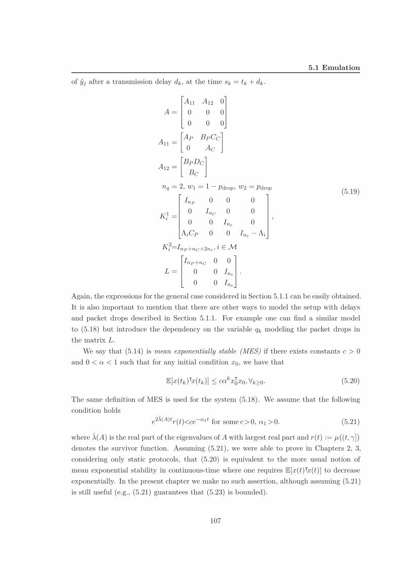
5.1 Emulation
of yj after a transmission delay dk, at the time sk = tk + dk.
A =
0
112
A11 A12 00 0 00 0 0
3
445
A11 =#AP BP CC
0 AC
$
A12 =#BP DC
BC
$
nq = 2, w1 = 1 0 pdrop, w2 = pdrop
K1i =
0
111112
InP 0 0 00 InC 0 00 0 Ine 0
&iCP 0 0 Ine 0 &i
3
444445,
K2i =InP +nC+2ne , i + M
L =
0
112
InP +nC 0 00 0 Ine
0 0 Ine
3
445 .
(5.19)
Again, the expressions for the general case considered in Section 5.1.1 can be easily obtained.It is also important to mention that there are other ways to model the setup with delaysand packet drops described in Section 5.1.1. For example one can find a similar modelto (5.18) but introduce the dependency on the variable qk modeling the packet drops inthe matrix L.
We say that (5.14) is mean exponentially stable (MES) if there exists constants c > 0and 0 < $ < 1 such that for any initial condition x0, we have that
E[x(tk)!x(tk)] ! c$kx!0x0, 2k$0. (5.20)
The same definition of MES is used for the system (5.18). We assume that the followingcondition holds
e2$(A)tr(t)<ce!!1t for some c>0, $1 >0. (5.21)
where "(A) is the real part of the eigenvalues of A with largest real part and r(t) := µ'(t, .]
(
denotes the survivor function. Assuming (5.21), we were able to prove in Chapters 2, 3,considering only static protocols, that (5.20) is equivalent to the more usual notion ofmean exponential stability in continuous-time where one requires E[x(t)!x(t)] to decreaseexponentially. In the present chapter we make no such assertion, although assuming (5.21)is still useful (e.g., (5.21) guarantees that (5.23) is bounded).
107

5. DYNAMIC PROTOCOLS
5.1.2 Main Results
For simplicity, we assume in Subsection 5.1.2.1 and 5.1.2.2, that there are no delays, i.e.,dk = 0, 2k, and no packet drops, i.e., pdrop = 0, and in Subsection 5.1.2.3 we consider thegeneral case.
5.1.2.1 Stability Result I and dynamic vs. static protocols
The following is our first stability result for (5.14).
Theorem 36. The system (5.14) with dynamic protocol (5.15) is MES if there exist scalars{0 ! pji ! 1, j, i + MD}, with !mD
j=1 pji = 1, 2i&MD , and nx # nx symmetric matrices{Ri > 0, i + MD} such that
J!d1(i)(
mD*
j=1pjiE(Rj))Jd1(i) 0 Ri < 0, 2i&MD , (5.22)
whereE(Rj) :=
) +
0eA!hRjeAhµ(dh). (5.23)
"
This result can be used to analyze if a given protocol yields the networked controlsystem stable or to synthesize a protocol that achieves this.Analysis: Note first that a given dynamic protocol specified by Ri > 0, i + MD, is equiva-lent to a dynamic protocol specified by
Ri = P + Ri > 0, i + MD, (5.24)
where P can be any symmetric matrix such that P + Ri > 0. If we replace in (5.22) thematrices Ri by Ri, given by (5.24), we obtain that (5.22), (5.24) are LMIs in the variablesP and pji (using the fact that !m
j=1 pji = 1, 2i&MD ).Synthesis: If we allow Ri to be variables in (5.22), then (5.22) are in general BMIs. In fact,if we chose a basis Bl for the linear space of symmetric matrices, we have Ri = !ns
l=1bilBl
and (5.22) depends on the products pjibil. In this case the dynamic protocol, determinedby the matrices Ri comes out from the solution to (5.22).
To state the next theorem, we need the following result which can be found in [AHS09b].Let [i] := i if i + {1, . . . , mS 0 1} and [i] = 1 if i = mS. Let MS := {1, . . . , mS}.
Theorem 37. The system (5.14), with static protocol (5.16) is MES if and only if thereexists nx # nx symmetric matrices {Ri > 0, i + MS} such that
J!s(i)E(R[i+1])Js(i) 0 Ri < 0, 2i&MS (5.25)
where E(R[i+1]) is given as in (5.23).
108
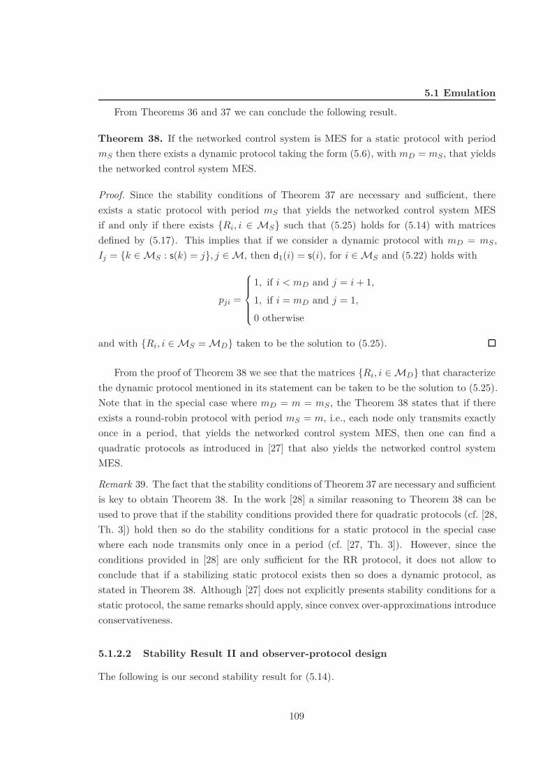
5.1 Emulation
From Theorems 36 and 37 we can conclude the following result.
Theorem 38. If the networked control system is MES for a static protocol with periodmS then there exists a dynamic protocol taking the form (5.6), with mD = mS, that yieldsthe networked control system MES.
Proof. Since the stability conditions of Theorem 37 are necessary and su"cient, thereexists a static protocol with period mS that yields the networked control system MESif and only if there exists {Ri, i + MS} such that (5.25) holds for (5.14) with matricesdefined by (5.17). This implies that if we consider a dynamic protocol with mD = mS ,Ij = {k + MS : s(k) = j}, j + M, then d1(i) = s(i), for i + MS and (5.22) holds with
pji =
+:::,
:::-
1, if i < mD and j = i + 1,
1, if i = mD and j = 1,
0 otherwise
and with {Ri, i + MS = MD} taken to be the solution to (5.25).
From the proof of Theorem 38 we see that the matrices {Ri, i + MD} that characterizethe dynamic protocol mentioned in its statement can be taken to be the solution to (5.25).Note that in the special case where mD = m = mS , the Theorem 38 states that if thereexists a round-robin protocol with period mS = m, i.e., each node only transmits exactlyonce in a period, that yields the networked control system MES, then one can find aquadratic protocols as introduced in [27] that also yields the networked control systemMES.
Remark 39. The fact that the stability conditions of Theorem 37 are necessary and su"cientis key to obtain Theorem 38. In the work [28] a similar reasoning to Theorem 38 can beused to prove that if the stability conditions provided there for quadratic protocols (cf. [28,Th. 3]) hold then so do the stability conditions for a static protocol in the special casewhere each node transmits only once in a period (cf. [27, Th. 3]). However, since theconditions provided in [28] are only su"cient for the RR protocol, it does not allow toconclude that if a stabilizing static protocol exists then so does a dynamic protocol, asstated in Theorem 38. Although [27] does not explicitly presents stability conditions for astatic protocol, the same remarks should apply, since convex over-approximations introduceconservativeness.
5.1.2.2 Stability Result II and observer-protocol design
The following is our second stability result for (5.14).
109
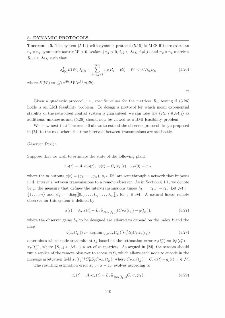
5. DYNAMIC PROTOCOLS
Theorem 40. The system (5.14) with dynamic protocol (5.15) is MES if there exists annx # nx symmetric matrix W > 0, scalars {cij > 0, i, j + MD, i 1= j} and nx # nx matricesRi, i + MD such that
J!d(i)E(W )Jd(i) +
mD*
j=1,j +=i
cij(Rj 0 Ri) 0 W < 0, 2i&MD (5.26)
where E(W ) :=" +
0 (eAh)!W eAhµ(dh).
"
Given a quadratic protocol, i.e., specific values for the matrices Ri, testing if (5.26)holds is an LMI feasibility problem. To design a protocol for which mean exponentialstability of the networked control system is guaranteed, we can take the {Ri, i + MD} asadditional unknowns and (5.26) should now be viewed as a BMI feasibility problem.
We show next that Theorem 40 allows to extend the observer-protocol design proposedin [24] to the case where the time intervals between transmissions are stochastic.
Observer Design
Suppose that we wish to estimate the state of the following plant
xP (t) = AP xP (t), y(t) = CP xP (t), xP (0) = xP 0
where the m outputs y(t) = (y1, . . . , ym), yi + Rsi are sent through a network that imposesi.i.d. intervals between transmissions to a remote observer. As in Section 5.1.1, we denoteby µ the measure that defines the inter-transmissions times hk := tk+1 0 tk. Let M :={1 . . . , m} and $j := diag([0s1 , . . . , Isj , . . . , 0sm ]), for j + M. A natural linear remoteobserver for this system is defined by
˙x(t) = AP x(t) + Lk$c(xe(t!k ))(CP x(t!
k ) 0 y(t!k )), (5.27)
where the observer gains Lk to be designed are allowed to depend on the index k and themap
c(xe(t!k )) := argminj&Mxe(t!
k )!C!P SjCP xe(t!
k ) (5.28)
determines which node transmits at tk based on the estimation error xe(t!k ) := xP (t!
k ) 0xP (t!
k ), where {Sj , j + M} is a set of m matrices. As argued in [24], the sensors shouldrun a replica of the remote observer to access x(t), which allows each node to encode in themessage arbitration field xe(t!
k )!C!P SjCP xe(t!
k ), where CP xe(t!k ) = CP x(t)0yj(t), j + M.
The resulting estimation error xe := x 0 xP evolves according to
xe(t) = AP xe(t) + Lk$c(xe(t!k ))CP xe(tk). (5.29)
110

5.1 Emulation
We can cast this problem into the framework of (5.14) with dynamic protocol (5.15) byadding an auxiliary variable v that holds the value of xe(tk) between transmission times,considering x = (xe, v) and
A =#
AP InP
0nP 0nP
$
,
Ji =#
InP 0nP
0nP 0nP
$
+#
0Lk
$ %$iCP 0
&
Ri =#C!
P SjCP 00 0nP
$
. (5.30)
In the following theorem, we propose a method to obtain observer gains Lk that yieldthe networked control system MES. To state the result we need the following assumption:
H(s) :=) s
0eAP rdr is invertible for every s+ [0, .] (5.31)
While this assumption holds generically, it is possible to construct examples where it does
not, as in the case where . > s = 23 and AP =#
0 101 0
$
, in which case H(s) = 0.
Theorem 41. Suppose that (5.31) hold. If there exists a nP # nP symmetric matrixP > 0, a m # m matrix Y , a nP # m matrix M , m # m matrices {Si, i + M}, and scalars{cij > 0, i, j + M}, such that
F (P ) + DM$iCP + (DM$iCP )! + C!P Y CP + (5.32)
m*
j=1,j +=i
cij(C!P SjCP 0 C!
P SiCP ) 0 P < 0, 2i&M
#P M
M! Y
$
> 0, (5.33)
where F (P ) :=" +
0 eA!P rPeAP rµ(dr) and D :=
" +0 eAP rµ(dr), then we have that the observer
gain Lk = H(hk)!1P !1M yields (5.14) with matrices (5.30) MES.
"
Note that our proposed observer gain Lk depends on the length hk of the time interval{tk+1 0 tk}, which is not known at time tk ! t ! tk+1 (5.27). In practice this results in adelay in constructing the state estimate that never needs to exceed hk since the state ofthe remote observer (5.27) can only be updated with the measurement y(tk) at the timetk+1 at which hk can be computed.
Similarly to the Theorem 40, the conditions of the Theorem 41 can be used to investigatethe stability of a given protocol determined by matrices Rj , in which case the problem
111

5. DYNAMIC PROTOCOLS
reduces to an LMI feasibility problem, or they can be used to design a protocol, in whichcase one needs to solve a BMI feasibility problem.
Remark 42. When the intervals between transmission are constant, one can show that thestability conditions (5.32) and (5.33) are equivalent to the ones given in [24], where such anassumption is made. In this case, the matrices Lk do not depend on k, and can thereforebe computed o!-line.
5.1.2.3 Extensions to handle delays and packet drops
Theorems 40 and 36 can be extended to the case where the network introduces packetdrops and delays modeled by (5.18) with matrices (5.19). We state these extensions next.
Theorem 43. The system (5.18) with dynamic protocol (5.15) is MES if there exist scalars{0 ! pji ! 1, j, i + MD}, with !mD
j=1 pji = 1, 2i&MD , and nx # nx symmetric matrices{Ri > 0, i + MD} such that
nq*
l=1wl
'K l
d1(i)!(
mD*
j=1pjiE(Rj))K l
d1(i)(
0 Ri < 0, 2i&MD ,
where
E(Rj) :=) +
0
) h
0(eAh!sLeAs)!RjeAh!sLeAs/(dh, ds). (5.34)
"
Theorem 44. The system (5.18) with dynamic protocol (5.15) is MES if there exists annx # nx symmetric matrix W > 0, scalars {cij > 0, i, j + MD, i 1= j} and nx # nx matricesRi, i + MD such that
nq*
l=1wl(K l
d1(i))!E(W )K ld1(i) +
m*
j=1,j +=i
cij(Rj 0 Ri) 0 W < 0,
2i&MD , where E(W ) is defined as in (5.34).
5.1.3 Illustrative Example
In this section we show that Theorems 40 and 44 reduce the conservatism of the resultsin [44], [87] and [27]. These three works use the same benchmark problem for the controlof a batch reactor, where the plant (5.36) and controller (5.2) matrices are given by
112

5.1 Emulation
AP =
0
1112
1.38 00.2077 6.715 05.67600.5814 04.29 0 0.675
1.067 4.273 06.654 5.8930.048 4.273 1.343 02.104
3
4445,
BP =
0
1112
0 05.679 01.136 03.1461.136 0
3
4445, CP =
#1 0 1 010 1 0 0
$.
AC =#
0 00 0
$,BC =
#0 11 0
$,CC =
#02 00 8
$,DC =
#0 025 0
$.
Only the two outputs are sent through the network, i.e., u(t) = u(t). The networkimposes i.i.d. intervals between transmissions, possibly packet drops and no delays. Thenetworked control closed loop can be written as in (5.14), (5.17) in the absence of drops andas in (5.18)- (5.19) when drops occur. Thus, the stability of the networked control systemcan be tested by Theorems 36, 40, and 43, 44. The results are shown in the Table 5.1,considering two distributions µ for the inter-transmissions intervals hk: uniform in theinterval [0, .], and exponential with expected value 1/"exp.
Table 5.1: Stability results for the batch reactor example-MEF-TOD and Round Robinprotocol. NA stands for Not Available
Dynamic Protocol Static Protocolno drops p = 0.5 no drops p = 0.5
Max. + : hk / Uni.(+)Results from [88] NA NA NA NAResults from [44] 0.0372 0.0170 0.0517 0.0199Results from [27] 0.11 NA NA NAThs. 40 and 44 0.0550 0.024 NA NAThs. 36 0.111 NA NA NATh. 37 NA NA 0.112 0.0385
Max. 1/$exp :hk / Exp.($exp)
Results from [88] 0.0095 0.0046 NA NAResults from [44] 0.0158 0.00795 0.0217 0.00924Results from [27] NA NA NA NAThs. 40 and 44 0.0226 0.01124 NA NAThs. 36 0.0357 NA NA NATh. 37 NA NA 0.0417 0.0188
From Table 5.1 we can conclude that our results allow to significantly reduce the con-servatism of the conditions in [44] and [88] for the same benchmark examples. The resultsin [27] are very close to the ones obtained with Theorem 36 and both outperform the resultsobtained with Theorem 40.
In Table 5.2, we show the results obtained by allowing Ri in Theorem 36 to be additional
113

5. DYNAMIC PROTOCOLS
variables, i.e., the protocol is to be designed. Note that Theorem 38 assures that thevalues obtained with Theorem 36 for the maximum support of a uniform distribution thatpreserves stability when a dynamic protocol (obtained from solving (5.22)) is utilized, arelarger than the ones obtained with the necessary and su"cient conditions provided byTheorem 37 for the static protocol, which matches well with the results in Table 5.2.
Table 5.2: Stability results for the batch reactor example-Protocol design, no packet dropsDynamic Prot. Design (Th.36) Static Prot. (Th.37)
Max.+ :hk/Uni.(+) 0.140 0.112
5.2 Direct Design
5.2.1 Problem Formulation
For the direct design problem 1 we assume, for simplicity, evenly spaced times betweentransmission, i.e., tk+1 0 tk = !s, 2k$0, for some sampling period !s, and we assume thatthere are no packet drops and no delays. We introduce the scheduling sequence
,(k) + M, for k + K, (5.35)
which indicates that at the time tk, ,(k) is the node that transmits, where K := {0, . . . , kF },with kF + N : {/}, denotes the set of the time instants of interest. In this case, if we letx[k] = xP (t!
k ), the discretization of the model for the plant 5.36 at times tk is given by
x[k + 1] = Ax[k] + Bu[k]y[k] = Cx[k]
(5.36)
where A = eAP *s , B =" *s
0 eAP sdsBP and C = CP , and y[k] = y(t!k ), u[k] = u(t!
k ).However, to directly take into account the communication constraints imposed by thenetwork, and to consider external disturbances acting on the plant we consider
x[k + 1] = Ax[k] + B)"(k)u[k] + wx[k], k " 0y[k] = ("(k)Cx[k] + wy[k]
(5.37)
where )j and (j , j + M are given in (5.11) and (5.11). The vectors wx[k] and vy[k]are zero mean independent Gaussian processes characterized by the covariance matricesE[wx[k]wx[k]!] = %x and E[wy[k]wy [k]!] = %y. The initial state x[0] is assumed to bea Gaussian variable, with E[x[0]] = x0, and E[x[0]x[0]!] = %0. Note that (5.37) indeedcaptures the fact that ,(k) selects at each time step k which components of the inputvector u[k] can influence the plant model, and which components of the output vector y[k]
1This Section was revised taking into account a follow-up work to the thesis [AHHS11a] and [AHHS11b]
114

5.2 Direct Design
are available for feedback. Moreover, we assume that when the actuation associated withactuator 1 ! j ! nu is not available it is set to zero throughout the interval [tk, tk+1),which is already captured in the model (5.37). Note that this model di!ers from the modelconsidered for there emulation approach, where we considered the input of the plant to beheld constant.
We are interested in the problem
min"(k),uk
E[kF !1*
k=0x[k]!Qx[k] + u[k]!Ru[k] + x[kF ]!Qx[kF ]] (5.38)
where the matrices Q and R are assumed to be positive definite. The set of admissiblecontrol laws u[k] is the set of functions of the information available to the controller fromlistening the network up to time tk, i.e., {y', u', + < k}.
Remark 45. Note that we do not need to impose the restrictions that uj[k] = 0 at timesat which the actuator j does not receive an update, since its value at these times doesnot a!ect (5.37). In fact, since uj [k] is always weighted in the performance cost it isautomatically set to zero at these times by the optimal and suboptimal controllers thatwe propose in the sequel (cf. Remark 42). Likewise, we do not need to assume that thecontroller does not know yi[k] at times at which sensor i does not send data to the controller.In fact, yi[k] is purely noise at these times, and it is automatically not taken into accountby the optimal and suboptimal controllers that we propose in the sequel (cf. Remark 42).
5.2.2 Main Results
In this section, we start by showing how to compute the cost (5.38) for a periodic basepolicy and then we present the scheduling protocol that a rollout policy with this periodicbase policy leads to.
5.2.2.1 Base Policy
To defined a periodic scheduling, we consider a set of h consecutive schedules for ,(k)denoted by
(v0, . . . , vh!1), (5.39)
where v' + M, 0 ! + ! h 0 1, which are periodically repeated as explained next. If we let<k=h denote the remainder after division of k by h, we have
,(k) = #&k , k + {0, . . . , kF }, (5.40)
where#&
k := v0k+&1h, k " 0, (5.41)
115
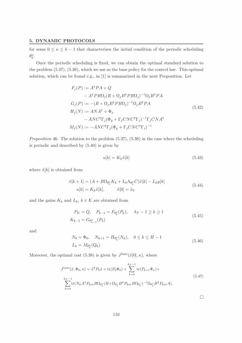
5. DYNAMIC PROTOCOLS
for some 0 ! ) ! h 0 1 that characterizes the initial condition of the periodic scheduling#&
k .Once the periodic scheduling is fixed, we can obtain the optimal standard solution to
the problem (5.37), (5.38), which we use as the base policy for the control law. This optimalsolution, which can be found e.g., in [1] is summarized in the next Proposition. Let
Fj(P ) := A!PA + Q
0 A!PB)j(R + )jB!PB)j)!1)jB!PA
Gj(P ) := 0(R + )jB!PB)j)!1)jB
!PA
Hj(N) := ANA! + %x
0 ANC!(j(%y + (jCNC!(j)!1(jCNA!
Mj(N) := 0ANC!(j(%y + (jCNC!(j)!1
(5.42)
Proposition 46. The solution to the problem (5.37), (5.38) in the case where the schedulingis periodic and described by (5.40) is given by
u[k] = Kkx[k] (5.43)
where x[k] is obtained from
x[k + 1] = (A + B)2"kKk + Lk&2"
kC)x[k] 0 Lky[k]
u[k] = Kkx[k], x[0] = x0(5.44)
and the gains Kk and Lk, k + K are obtained from
PK = Q, Pk!1 = F2"k(Pk), kF 0 1 " k " 1
Kk!1 = G2"k!1
(Pk)(5.45)
andN0 = %0, Nk+1 = H2"
k(Nk), 0 ! k ! H 0 1
Lk = M2"k(Qk)
(5.46)
Moreover, the optimal cost (5.38) is given by Jbase(x[0], )), where
Jbase(x, %0, )) = x!P0x + tr(P0%0) +kF !1*
k=0tr(Pk+1%x)+
kF !1*
k=0tr(NkA!Pk+1B)$"
k(R+)$"
kB!Pk+1B)$"
k)!1)$"
kB!Pk+1A).
(5.47)
"
116

5.2 Direct Design
5.2.2.2 Rollout Policy
We propose to choose at each iteration the control law and the node to transmit as theones that leads to optimal performance over a fixed lookahead horizon, assuming that fromthen on a periodic base policy is used. In other words, at each iteration +, 0 ! + ! kF 0 1,the schedules
,(+), ,(+ + 1), . . . , ,(+ + H 0 1)
and the controlsu[+], u[+ + 1], . . . , u[+ + H 0 1]
are assumed to be free variables, where H denotes the length of the lookahead horizon,while
,(+ + H), ,(+ + H + 1), . . .
andu(+ + H), u(+ + H + 1), . . .
are fixed and follow a periodic policy as in (5.40), (5.41), and (5.56), (5.44). The freescheduling variables are denoted by ' = ('0, . . . , 'H!1), i.e.,
,(k) = 'k!', for k + {+, . . . , + + H 0 1} (5.48)
and the fixed scheduling variables can be written as
,(k) = #&k!('+H), for k + {+ + H, . . . , kF 0 1}. (5.49)
Note that at time + + H the base policy is assumed to start at an initial schedule v&,determined by ). We consider that ) + {0, . . . , h 0 1} is also a decision variable, and thedecision set is denoted by I := MH # {0, . . . , h 0 1}, i.e, (', )) + I. The length of thelookahead horizon is a fixed constant, but naturally needs to be adapted when the iterationstep is close to the terminal step time kF , i.e,
H(+) := min(Hc, kF 0 1 0 +), (5.50)
where 1 ! Hc ! kF 0 1 is a constant. The dependency of H on + is omitted hereafter. Theprocess is restarted at each step.
As we shall see in the sequel this procedure boils down to the following protocol.
Protocol 1. Given the data {yk, uk, k < +} obtained by listening to the network, at eachiteration + choose
,(+) = ''0, (5.51)
where ''0 is the first entry of the vector '' = (''0, . . . , ''H!1) obtained from
('', )')=argmin(0,&)&I x!' P0,&,'x'+((', ), +)+1(', ), +, N'), (5.52)
and the quantities in (5.52) are determined as follows.
117
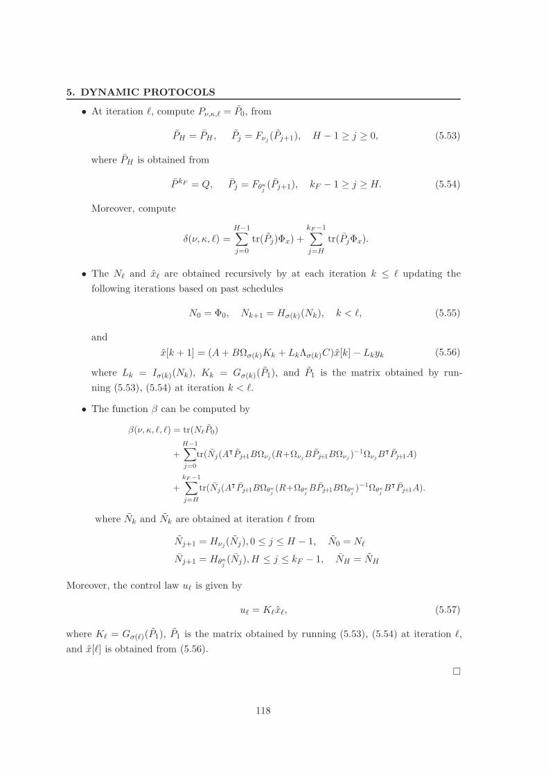
5. DYNAMIC PROTOCOLS
• At iteration +, compute P0,&,' = P0, from
PH = PH , Pj = F0j (Pj+1), H 0 1 " j " 0, (5.53)
where PH is obtained from
P kF = Q, Pj = F2"j(Pj+1), kF 0 1 " j " H. (5.54)
Moreover, compute
((', ), +) =H!1*
j=0tr(Pj)%x) +
kF !1*
j=H
tr(Pj%x).
• The N' and x' are obtained recursively by at each iteration k ! + updating thefollowing iterations based on past schedules
N0 = %0, Nk+1 = H"(k)(Nk), k < +, (5.55)
andx[k + 1] = (A + B)"(k)Kk + Lk&"(k)C)x[k] 0 Lkyk (5.56)
where Lk = I"(k)(Nk), Kk = G"(k)(P1), and P1 is the matrix obtained by run-ning (5.53), (5.54) at iteration k < +.
• The function 1 can be computed by
1(', ), +, +) = tr(N"P0)
+H!1*
j=0tr(Nj(A!Pj+1B)%j (R+)%j BPj+1B)%j )!1)%j B!Pj+1A)
+kF !1*
j=H
tr(Nj(A!Pj+1B)$"j(R+)$"
jBPj+1B)$"
j)!1)$"
jB!Pj+1A).
where Nk and Nk are obtained at iteration + from
Nj+1 = H0j(Nj), 0 ! j ! H 0 1, N0 = N'
Nj+1 = H2"j(Nj), H ! j ! kF 0 1, NH = NH
Moreover, the control law u' is given by
u' = K'x', (5.57)
where K' = G"(')(P1), P1 is the matrix obtained by running (5.53), (5.54) at iteration +,and x[+] is obtained from (5.56).
"
118
5.2 Direct Design
As stated next, this protocol does in fact correspond to the rollout algorithm describedabove, and it always outperforms the corresponding periodic base policy.
Theorem 47. The rollout scheduling algorithm with the base policy described in Subsec-tion 5.2.2.1 is determined by the Protocol 1. Moreover
Jdyn(x, %) ! min0*&*k!1
Jbase(x, %, )) (5.58)
where Jdyn(x) is the cost (5.38) when the scheduling sequence ,(k) and the control law uk
for the system (5.37) are as described by Protocol 1, starting with an initial state estimatex0 = x and associated covariance matrix %0 = %.
"
The Protocol 1 can be implemented in the nodes of the network in a distributed way. Infact every node can listen to the network at each transmission time, and therefore computex', and also Q', at time t'. In fact, knowing the data sent over the network at times{tk < t', k " 0}, nodes can locally iterate (5.56) and (5.55). Moreover, since the knowledgeof x', and also Q', at time t' is all one needs to run the Protocol (1), each node canimplement the same rollout algorithm independently and therefore determine which nodeis the next to transmit. At each transmission step, the node that gains arbitration simplytransmits and the other nodes do not. This implementation does not assume anythingfrom the network, e.g., whether it is wired or wireless, besides from the fact that the nodeshave the ability to listen to other nodes messages. This contrasts to, e.g., the solutionproposed in [91] for CAN-BUS networks where the assumption that we have available anarbitration field that is used in the network messages plays an essential role.
Another important observation, is that every information that the nodes require tocompute the arbitration function (5.52) is available at time t'!1 and therefore computationscan be done between time t'!1 and t', in a way that there are no delays at time t'. Thefeasibility of this implementation depends on the computational capacity of the nodes, i.e.,whether they can perform these calculations in a time interval no larger than one samplinginterval h.
Remark 48. The equations (5.56) and (5.57). confer what was stated intuitively in Re-mark 42. In fact, if an actuator 1 ! i ! m does not receive an update at time t' thenthe corresponding entries of the matrix )"(') is zero, and from the structure of the gainsK' = G"(')(P1) where G is defined in (5.42) we also have that uj[k] = 0. Likewise, if asensor 1 ! i ! ny does not transmit at time t' then the corresponding entries of the matrix("(') is zero, and from the structure of the gains L' = I"(')(N') where I is defined in (5.42)we have that yj = 0 is not taken into account in (5.56).
119
5. DYNAMIC PROTOCOLS
5.2.3 Illustrative Example
Consider the problem of controlling an inverted pendulum by a remote controller, whichis connected to the pendulum system though a communication network as the CAN-BUS,Wireless 802.11, or the Ethernet. Thus, the controller has to choose at each transmissiontime either to send a control action (torque) for the pendulum or obtain a measurement,which is assumed to be a measurement of the displacement angle. Control decisions attime tk correspond to ,(k) = 1, and measurement decision to ,(k) = 2. We assumethat transmissions occur with a sampling period of !s = 0.1. A discretized model ofa linearization of the inverted pendulum about the unstable equilibrum point is givenby (5.37), with
A = eAP *s , B =) *s
0eAP sBP ds, C = [1 0],
where
AP =#0 11 0
$
, BP =#01
$
,
and (1 = 0, (2 = 0, )1 = 1, )2 = 0. The noise signals in (5.37) are characterized by
%0 = 0.1I2, , %x = 0.001I2, %y = 0.001
The performance criterium is given,
E[kF !1*
k=0(Cx[k])2 + u[k]2dt + (Cx[kF ])2] (5.59)
with kF = 100 and the controller aims at finding simultaneously the scheduling sequence,(k) and the control law uk that minimize (5.59).
Consider for the base policy a periodic scheduling law that alternates between samplingand control, i.e, with period 2. We can compute from Proposition 46 the cost (5.59) whenthis periodic scheduling and the optimal control law given in Proposition 46 are appliedto (5.37) with the matrices described above. However, we have no closed-form solution tocompute the cost (5.59) when the scheduling is obtained by running the Protocol 1. Thus,we estimate it by running Monte Carlo simulations of the protocol. The results for thebase and rollout policies are shown in Table 5.3. The cost for the base policy can alsobe confirmed by running Monte Carlo simulations. The values in Table 5.3 corroborateTheorem 47, i.e., the cost obtained with the rollout policy is less than the one obtainedwith the base policy. In fact, a significant improvement of about 22 percent of the basepolicy cost is achieved.
120
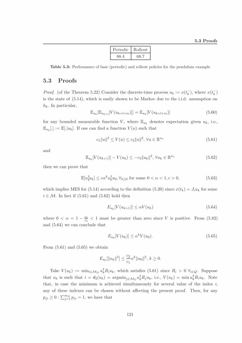
5.3 Proofs
Periodic Rollout88.4 68.7
Table 5.3: Performance of base (periodic) and rollout policies for the pendulum example
5.3 Proofs
Proof. (of the Theorem 5.22) Consider the discrete-time process uk := x(t!k ), where x(t!
k )is the state of (5.14), which is easily shown to be Markov due to the i.i.d. assumption onhk. In particular,
Euk [Euk+l [V (uk+l+m)]] = Euk [V (uk+l+m)] (5.60)
for any bounded measurable function V , where Euk denotes expectation given uk, i.e.,Euk [.] := E[.|uk]. If one can find a function V (u) such that
c1)u)2 ! V (u) ! c2)u)2, 2u + Rnx (5.61)
andEuk [V (uk+1)] 0 V (uk) ! 0c3)uk)2, 2uk + Rnx (5.62)
then we can prove that
E[u!kuk] ! c$ku!
0u0, 2k$0 for some 0 < $ < 1, c > 0. (5.63)
which implies MES for (5.14) according to the definition (5.20) since x(tk) = Jiuk for somei + M. In fact if (5.61) and (5.62) hold then
Euk [V (uk+1)] ! $V (uk) (5.64)
where 0 < $ = 1 0 c3c2
< 1 must be greater than zero since V is positive. From (5.82)and (5.64) we can conclude that
Eu0 [V (uk)] ! $kV (u0). (5.65)
From (5.61) and (5.65) we obtain
Eu0 [)uk)2] ! c2c1
$k)u0)2, k " 0.
Take V (uk) := mini&MD u!kRiuk, which satisfies (5.61) since Ri > 0 2i&Q. Suppose
that uk is such that i = d2(uk) = argminj&MDu!
kRjuk, i.e., V (uk) = min u!kRiuk. Note
that, in case the minimum is achieved simultaneously for several value of the index i,any of these indexes can be chosen without a!ecting the present proof. Then, for anypji " 0 : !mD
j=1 pji = 1, we have that
121
5. DYNAMIC PROTOCOLS
Euk [V (uk+1)] =Euk [ min
j&MD
u!kJ!
d1(i)eA!hRjeAhJd1(i)uk]
! Euk [mD*
j=1pjiu
!kJ!
d1(i)eA!hRjeAhJd1(i)uk]
= u!kJ!
d1(i)
mD*
j=1pjiE(Rj)Jd1(i)uk (5.66)
Suppose we choose pji such that (5.22) holds, i.e.,
J!d1(i)
mD*
j=1pjiE(Rj)Jd1(i) 0 Ri = 0Qi
for some Qi > 0. Then from (5.66) we conclude that Euk [V (uk+1)]0V (uk) ! 0u!kQiuk, i =
d2(uk), which implies (5.62) and concludes the proof.
Proof. (of the Theorem 40) As in the proof of the Theorem 36 it su"ces to find a functionV (uk) such that (5.61), (5.62) hold. Take V (uk) = u!
kW uk, where W is the solutionto (5.26) and suppose that i = argminj&Mu!
kRjuk. Then
Euk [V (uk+1)] 0 V (uk) = u!k[J!
d1(i)E(W )Jd1(i) 0 W ]uk,
=0u!k[
mD*
j=1,j +=i
cij(Rj 0 Ri) + Qi]uk
(5.67)
where Qi > 0. Since i = argminj&Mu!kRjuk we have that u!
k[!mDj=1,j +=i cij(Rj 0 Ri)]uk " 0
for every uk + %nx and therefore from (5.67) we conclude that V satisfies (5.62). It is alsoclear that V satisfies (5.61), which concludes the proof.
Proof. (of the Theorem 41) We start by noticing that if there exists P > 0 such that) +
0[eAP h+H(h)Lk$iCP )!P (eAP h+H(h)Lk$iCP ]µ(dh) (5.68)
+m*
j=1,j +=i
cij(C!P SjCP 0 C!
P SiCP ) 0 P < 0
then (5.26) holds for (5.14) with matrices (5.30). In fact, since m = mDP , we can assumethat d1(i) = i, 2i&M since if this is not the case we can relabel the sensor nodes in such away this holds. Noticing that for A, Ji given by (5.30) we have that
eAhJi =#eAP h + H(h)Lk$iC 0
Lk$iC 0
$
.
122

5.3 Proofs
We can prove that (5.26) holds for W = diag([P %InP ]) since in this case (5.26) takes theform
) +
0
#B(h) 0
0 0
$
+m*
j=1,j +=i
cij
#C!
P SjCP 0 C!P SiCP 0
0 0nP
$
0#P 00 %InP
$
< 0, 2i&M (5.69)
where
B(h)=(eAP h+H(h)Lk$iCP )!P (eAP h+H(h)Lk$iCP ) (5.70)+%(Lk$iCP )!(Lk$iCP ) (5.71)
Thus if (5.68) holds then (5.69) holds for su"ciently small %. Set Lk = H(hk)!1P !1M fora nP # m matrix. Then (5.68) can be written as
F (P ) + DM$iCP + (DM$iCP )! + C!P MP !1MCP +
m*
j=1,j +=i
cij(C!P SjCP 0 C!
P SiCP ) 0 P < 0, 2i&M(5.72)
If we let Y > 0 be such that M!P !1M < Y , which applying the Shur complement canbe seen to be equivalent to (5.33), we see that if (5.32) holds then (5.72) holds, whichconcludes the proof.
5.3.1 Proof of Theorem 5.3.1
For simplicity we restrict the proof to the case where µ is absolutely continuous, i.e.,µ([0, t)) =
" t0 f(s)ds where f is a probability density function.
Let ! := t0 tk be a variable that keeps track of the time elapsed since the last transmis-sion time tk. Then the pair x = (x, !) is a Piecewise Deterministic Process (PDP) in thesense of [25], where x is the state of (5.14). A PDP is a process where randomness comesinto play at fixed or random jump times but there is no source of uncertainty between thesetimes. In the present case these times are tk. A PDP can be described by three ingredients:(i) a deterministic flow, which describes the evolution of the state between jump times. Inthe present case this is the linear dynamics of (5.14); (ii) a possibly state-dependent tran-sition jump intensity which determines the occurrences of the jump times. In the presentcase the transitions intervals are independent and identically distributed, and therefore,at time t, the transition intensity depends on the time of the last jump before t and isgiven by the hazard function of f , "(!) := g(!)/s(!) where s(!) is the survivor functions(!) =
" +* f(r)dr [25]; (iii) a transition probability measure Q(x, dy) over the state-space
that characterizes the probability of a jump from a state to another state at jump times. In
123
5. DYNAMIC PROTOCOLS
the present case the transitions are state-dependent but deterministic and can be describedby the characteristic distribution
Prob[x(tk) + A|E] =)
AQ(x(t!
k ), dy) (5.73)
=
+:::,
:::-
1 if Jjx(t!k ) + A and
x(t!k )!Rjx(t!
k ) " x(t!k )!Rix(t!
k ), i + M
0 otherwise, (5.74)
where E is the event that a jump occurred at time tk and that the state is x(t!k ).
In [25], an expression is given for the extended generator A of a PDP and a characteri-zation is given for its domain, which consists of the class of functions for which
Ex0(V (x(t)))=V (x(0))+Ex0
) t
0AV (x(s))ds, 2t$0, (5.75)
where Ex0 denotes expectation given that the process started at the initial state x0 = x(0).We see from (5.75) that the extended generator for PDPs plays the role of a Lyapunovderivative for deterministic systems. The expression for the extended generator A takesthe form
AV (x) :=XV (x) + "(!)[V (Jjx, 0) 0 V (x)], (5.76)if x!Rjx ! x!Rix, i + M
where XV (x) := !i
,V (x),xi
xi.The following result will be key to prove Theorem 40. The proof is analogous to the
proof of the su"ciency part of the Theorem 24, and therefore it is omitted.
Theorem 49. If there exists a di!erentiable positive function V (x) which equals zero atzero, and positive constants c1, c2, k such that for every x = (x, !),
c1)x)2 ! V (x) ! c2)x)2 (5.77)AV (x) ! 0k)x)2 (5.78)
where AV (x) is given by (5.76) then the system (5.14) is MES.
"
Proof. (of Theorem 40) We start by noticing that (5.26) is equivalent to existing P > 0,U > 0, cij > 0 and Ri, i, j + M such that
E(W ) 0 U < 0 (5.79)
J!i UJi +
m*
j=1,j +=i
cij(Ri 0 Rj) 0 W < 0, 2i&M. (5.80)
124
5.3 Proofs
To see that (5.79) and (5.80) imply (5.26) note that (5.79) implies that J!i (E(W )0U)Ji < 0
for every i + M and adding this last equation to (5.80) for each i one obtains (5.26).Conversely, if (5.26) holds, U = E(W ) + %I satisfies (5.79) and (5.80) for su"ciently small%.
We consider a function V (x) = x!P (!)x, for a P (!) to be introduced shortly, and provethat V (x) satisfies the conditions of Theorem 49 provided that (5.79), (5.80) are satisfied.
Taking the generator of V (x) using (5.76) we obtain
AV (x) = x![P (!) + A!P (!) + P (!)A +"(!)(J!
j P (0)Jj 0 P (!))]xif x!Rjx " x!Rix, i + {1, . . . , m}
we shall show that there exists P (!) such that c1I < P (!) < c2I and
P (!) + A!P (!) + P (!)A + "(!)[J!i P (0)Ji 0 P (!))(5.81)
+ !mj=1 cij(Ri 0 Rj) + Zi] + Y = 0
for some matrices d1I < Zi < d2I, i + M, e1I < Y < e2I, to be introduced wherecl, dl, el, l + {1, 2} are positive constants. This implies that if we take such P (!) forV (x) = x!P (!)x then (5.61) takes the form
AV (x) = 0x![Y + "(!)(Zj + (m*
j=1cij(Ri 0 Rj)))]x
if x(t!k )!Rjx(t!
k ) " x(t!k )!Rix(t!
k ), i + {1, . . . , m}.
which implies that AV (x) = 0x!Y x, 2x&Rnx
Note that "(!) is a positive function. Thus, V (x) satisfies (5.77) and (5.78). If su"cesto prove that (5.79)-(5.80) implies that there exists c1I < P (!) < c2I, d1I < Zi < d2I,e1I < Y < e2I such that (5.81) holds.
Let P (0) = U , Zi = W 0 (!mj=1 cij(Ri 0 Rj) + J!
i P (0)Ji) > 0, where U, W, cij are thesolution to (5.79), (5.80). Moreover since from (5.79), E(W ) 0 U = 0Q for some Q > 0we can chose Y such that
" +0 eA!hY eAhf(h)dh = Q. Then the unique solution to (5.81) is
given by
P (!)=" +!*
0 eA!rW eAr f(*+r)s(*) dr (5.82)
+" +!*
0 eA!sY eAs s(*+s)s(*) ds
which can be confirmed by direct replacement. It is clear that P (!) is bounded and positivedefinite, and this concludes the proof.
125

5. DYNAMIC PROTOCOLS
5.4 Further Comments and References
Walsh and co-authors [90] made strides in the analysis of control systems closed via a localarea network, such as the controller-area network, the ethernet and wireless 802.11 net-works. The key assumptions in [90] are that there exists a bound on the interval betweentransmissions denoted by maximum allowable transfer interval (MATI), and that transmis-sion delays and packet drops are negligible. In [90] an emulation set-up is considered in thesense that the controller for the networked control system is obtained from a previouslydesigned stabilizing continuous-time controller. Two basic types of protocols have beenproposed: static protocols, such as the round-robin (RR) protocol where nodes take turnstransmitting data in a periodic fashion; and dynamic protocols such as the maximum errorfirst-try once discard (MEF-TOD) protocol, where the node that has the top priority in us-ing the communication medium is the one whose current value to transmit di!ers the mostfrom the last transmitted value. Under this setup, one can attempt to provide an upperbound on the MATI for which stability can be guaranteed. Since these protocols have beenproposed in the papers referenced above, MATI bounds have been improved [73], [88], [28].Although, [90] illustrate through simulations that using the MEF-TOD protocol allows forpreserving stability of the networked closed loop for a larger MATI than that obtainedwhen using the RR protocol, and similar conclusions are obtained in [73]- [28] from su"-cient stability conditions, no analytical result has been established proving that this holdsin general.
As mentioned in [90], the occurrence of transmission events on the network is oftenmore appropriately modeled as a random process. This feature is taken into accountin [44], which considers networked control systems with MEF-TOD and RR protocols,and independent and identically distributed (i.i.d.) intervals between transmissions. It isshown that stability can be guaranteed for distributions of the inter-transmission intervalsthat have a support larger than previously derived deterministic upper bounds for theMATI [90], [73], [88]. The conservativeness of these results for linear networked control sys-tems using the RR protocol was eliminated in [AHS09b]. Recently, [27] addresses a modelof networked control systems with i.i.d. intervals between transmissions and stochasticdelays for a class of quadratic protocols that is more general than MEF-TOD. Through aconvex over-approximation approach, su"cient conditions are given for mean exponentialstability. In [24] a method is proposed to design an observer-protocol pair to asymptoti-cally reconstruct the states of an LTI plant where the plants outputs are sent through anetwork with constant intervals between transmissions. The protocol to be designed canbe viewed as a weighted version of the MEF-TOD.
126

6
Output Regulation for Multi-rateSystems
One of the celebrated problems in automatic control, commonly known as output regula-tion, is that of controlling the output of a linear time-invariant system so as to achieveasymptotic tracking of an exogenous signal generated by the free motion of a linear time-invariant system, so-called exosystem, while guaranteeing closed loop stability. A solutionto this problem is required to yield closed-loop stability and should be such that outputregulation is achieved even in the presence of small plant uncertainties and exogenousdisturbances also generated by the exosystem.
In this chapter we address the output regulation problem for multi-rate systems. Multi-rate systems can arise in the scope of networked control system in cases where several nodesnegotiate fixed, but di!erent, bandwidths with the possibly several networks connectingthat are part of the networked control system. Networks that guarantee a fixed bandwith,are, for example, circuit switchign networks [58]. It can also simply represent a sensor,which outputs measurements at a fixed sampling rate, or an actuator which allows actuationupdates at a fixed rate. Typical cases of the use of multi-rate control systems design arisefrom hardware restrictions, for example, due to the fact that the discrete-analog (D/A)converters are generally faster than the analog-discrete (A/D) converters or from the useof camera-based sensors, which might require larger sampling periods than other sensorsand actuators ([35]). Another important application arises in the design of integratedguidance and control systems for vehicular applications ([ASC07], [ASC08b]), where thelinear positioning sensors (e.g. Global Positioning System (GPS)) are usually available ata lower rate than the remaining sensors.
We propose a controller that achieves stability for the closed loop and output regulationfor a number of regulated outputs equal to the number of inputs, while taking advantagesof the remaining outputs for feedback. Besides incorporating an internal model of the
127

6. OUTPUT REGULATION FOR MULTI-RATE SYSTEMS
exosystem, the key feature of our proposed controller is that it includes a system thatblocks signals generated by the exosystem arriving to the controller from the non-regulatedoutputs. The concept of a system that blocks signals is made precise, by introducing thenotion of blocking zero with respect to a matrix, both for LTI and periodic systems, whichgeneralizes the standard notion of blocking zero for LTI systems (see, e.g., [98]). We showthat there exists a stabilizing controller with the proposed structure, i.e., incorporatingan internal model of the exosystem and a system that blocks signals generated by theexosystem, that achieves output regulation even in the presence of plant uncertainties anddisturbances generated by the exosystem.
The remainder of the chapter is organized as follows. In Section 6.1, we provide theproblem setup and state the output regulation problem for multi-rate systems. In Sec-tion 6.2 we propose a solution to the problem statement summarized in our main result.An illustrative example showing that our solution allows to solve problems not possible tosolve through previous works is provided in Section 6.3. In Section 6.4 we introduce thenotion of blocking zero with respect to a matrix, which is a key concept to prove the mainresults which is established in Section 6.5. Further comments and references are given inSection 6.6.
6.1 Problem Formulation
We describe first the multi-rate set-up, and the exosystem. Then we state the outputregulation problem.
6.1.1 Multi-Rate Set-up
We consider a continuous-time plant#xP (t)yP (t)
$
=#AP BP
CP 0
$ #xP (t)uP (t)
$
+#EP
0
$
vP (t), t " 0, (6.1)
where xP (t) + Rn is the state, uP (t) + Rm is the input, and vP (t) + Rnv is a disturbancevector generated by the following system
wP (t) = SV wP (t), t " 0,
vP (t) = EV wP (t).(6.2)
The output vector yP (t) + Rp can be partitioned into
yP (t) = (y1P (t), . . . , y
ny
P (t))
where yiP (t) + Rpi , is associated with sensor i + {1, . . . , ny}, and !ny
i=1 pi = p. The sensorsare assumed to operate at di!erent sampling rates, with periods that are rationally related.
128
6.1 Problem Formulation
This model for the measurements can be described by
y[k] := (y1[k], . . . , yny [k]),
whereyi[k] := (i
kyiP (tk), k " 0, 1 ! i ! ny, (6.3)
tk := kts, for some ts > 0, (ik = .i
kIpi , and
.ik :=
+,
-1, if sensor i is sampled at tk
0, otherwise. (6.4)
Let(k := bdiag((1
k, . . . , (ny
k ).
Note that, due to our assumption that the periodicities of the sensors sampling are ratio-nally related, (k is a periodic function of k, i.e., there exists h such that (k = (k+h, 2k.We can assume that each diagonal entry of (k is non-zero at least once in a period sinceotherwise a given sensor component would never be sampled and could be disregarded.
The actuator mechanism is assumed to be a standard sample and hold device, and itis assumed to be available for update at every sampling time tk, i.e.,
u(t) = u[k], t + [tk, tk+1), (6.5)
where u[k] is the actuation update at time tk.Denote the sampled state at times tk by x[k] := x(tk). Then we can write (6.1), (6.3)
and (6.5) at times tk as
P :=< #
x[k + 1]y[k]
$
=#
A B
(kC 0
$ #x[k]u[k]
$
+#BV
0
$
v[k] (6.6)
where A = eAP h, B =" ts
0 eAP sdsBP , C = CP , BV =" ts
0 eA(ts!s)EP EV eSV sds, and v[k] =vP (tk) is generated by the discretization of (6.2), which is given by
wV [k + 1] = eSV tswV [k], k " 0,
v[k] = EV wV [k].(6.7)
6.1.2 Exosystem
Suppose that we further partition the output vector y[k] according to
y[k] =#ym[k]yr[k]
$
=#(mkCm
(rkCr
$
x[k] (6.8)
129

6. OUTPUT REGULATION FOR MULTI-RATE SYSTEMS
where (mk and (rk are nm # nm and m # m matrices, respectively, such that (k =bdiag((mk, (rk). Note that nm = p 0 m. The component yr[k] + Rm is a set of out-puts that we wish to asymptotically track a reference signal r[k], and ym[k] + Rpm is anadditional set of measurements available for feedback. Subsumed in this partition is thatp > m. A solution to the output regulation problem in the case where p ! m can be foundin [82].
The reference signal r[k] + Rm and the disturbance signal v[k] + Rnv are assumed tobe generated by the following model, which we denote by exosystem,
w[k + 1] = Sw[k]r[k] = CRw[k]v[k] = CV w[k],
(6.9)
where w[k] + Rnw . The matrices S and CV must be compatible with (6.7), i.e., the samesignal v[k] should be generated by (6.9) and (6.7). Consider the Jordan canonical form ofS i.e.,
S = V bdiag(S1, . . . , Sns)V !1 (6.10)where V is an invertible matrix and the matrices Sj take the form
Sj =
0
111112
µj 1 0 . . .
0 µj 1 . . .... ... . . . ...0 0 . . . µj
3
444445+ C&j#&j , 1 ! j ! ns (6.11)
where ns ! nw, and !nsj=1 )j = nw. We assume that:
(S1) )µi) " 1, 21*i*ns .
(S2) µi 1= µj for i 1= j.
To see that (S1) and (S2) introduce no loss of generality, note first that the exosystemcan generated signals r[k] and v[k] taking the form
*[k] =ns*
j=1
&j!1*
l=0bjl
=k
l
>
µk!lj , (6.12)
where bjl can be made arbitrarily by properly choosing CR, CV , and w[0]. Since, as we shallsee shortly, output regulation is an asymptotic property, if (S1) would not hold then thedisturbance and reference terms in (6.12) corresponding to stable eigenvalues of S wouldplay no role. If (S2) would not hold, the exosystem would still only be able to generatethe same class of reference and disturbance signals (6.12). Another way of stating (S2) isto say that the characteristic polynomial of S coincides with the minimal polynomial of S,which is a statement more commonly seen in related works addressing the internal modelprinciple (see, e.g., [13]).
130

6.2 Output Regulator for Multi-Rate Systems
Figure 6.1: Proposed controller structure to achieve output regulation; Plant:P; Controller:CI -internal model, CD blocking system, CK stabilizer
.
6.1.3 Problem Statement
Consider a linear controller for the system (6.6), i.e., a map y[k] ,- u[k] with state xc[k] +Rnc . We say that the closed-loop is stable if (x[k], xc[k]) - 0 as k - /, when r[k] = 0,2k$0. Moreover, we say that output regulation is achieved if (Crx[k]0r[k]) - 0 as k - /.
The problem we are interested in this chapter can be stated as follows.
Problem 50. Find a linear controller for the system (6.6) such that the closed loop is stableand output regulation is achieved.
6.2 Output Regulator for Multi-Rate Systems
The structure of the controller that we propose to solve the Problem 50 is shown in Fig-ure 6.1.
The purpose of the systems CI , CD and CK and the rationale behind this structure arebriefly explained as follows. Since the controller must provide the adequate input valueu[k] such that the output yr[k] of the linear plant tracks the desired reference signal r[k],the system CI is such that it is capable of providing such an input to the plant, when theinput to CI is identically zero. Denote by steady state the state of the plant at which outputregulation is achieved. At steady state, due to the linearity of the plant, the non-regulatedoutput ym[k] consists of a signal with the same frequency content of the input to the plant.The system CD has the purpose of yielding a zero output when the steady state signalym[k] is applied to its input, while assuring that other signals of interest, do not yield azero output and thus can still be utilized to control the plant.
Closed loop can be guaranteed if the following condition is met
(G1) The system ”seen” by the controller, i.e., obtained by computing the series of CI , Pand CD, with input yK [k] and output (yD[k], yr[k] 0 r[k]), is detectable and stabiliz-able.
131
6. OUTPUT REGULATION FOR MULTI-RATE SYSTEMS
In fact, from standard results for linear systems, if (G1) holds one can compute a stabilizingcontroller CK . Note that, when output regulation is achieved, both the input to thecontroller and its output are zero.
Before we state our main result, we provide possible choices for CI and CD. We shall im-pose in Section 6.5 some requirements that CI and CD must meet to prove our main outputregulation result. We shall see that the systems proposed below meet these requirements.However other choices may exist that satisfy these requirements.
6.2.1 System CI
The system CI is an LTI system described by
CI :=< #
xI [k + 1]yI [k]
$
=#AI BI
CI 0
$ #xI [k]uI [k]
$
(6.13)
where xI [k] + RnI , uI [k] + Rm, and yI [k] + Rm. The system CI should be capable ofproviding the adequate input to the plant such that output regulation is achieved. Such aninput takes the general form (6.12). One realization for (6.13) that achieves this is givenby
AI = bdiag(S, . . . , S) + R(mnw)#(mnw).
BI = bdiag(BJ , . . . , BJ) + R(mnw)#m
CI = bdiag(CJ , . . . , CJ) + Rm#(mnw) (6.14)
where BJ + RnI#1 is such that (S, BJ ) is stabilizable, and CJ + R1#nw is such that (CJ , S)is detectable. It is straightforward to verify that this implies that (AI , BI) is observable, and(CI , AI) is detectable, respectively (cf. Proposition 62 below). Note that, the system (6.13)with matrices (6.14) incorporates an m0fold reduplication of the exosystem (6.9), in thesense of [34].
6.2.2 System CD
The system CD , is a linear periodically time-varying system, described by
CD :=< #
xD[k + 1]yD[k]
$
=#ADk BDk
CDk DDk
$ #xD[k]uD[k]
$
(6.15)
where xD[k] + RnD , uD[k] + Rnm, and yD[k] + Rnm, and ADk, BDk, CDk and DDk areh0periodic, i.e., e.g., ADk = ADk+h, 2k$0.
The system CD has the purpose of blocking the signals that can be generated by theexosystem. By this we mean that the output of (6.15) is zero for every input generated
132
6.2 Output Regulator for Multi-Rate Systems
by the exosystem, which takes the general form (6.12). The notion is made precise in theAppendix (cf. Definition 58).
One realization for (6.15) that achieves this is given by
ADk = bdiag(A1k, . . . , Anm
k ) + Rnmnw#nmnw .
BDk = bdiag(B1k , . . . , Bnm
k ) + R(nmnw)#nm
CDk = bdiag(C1k , . . . , Cnm
k ) + Rnm#(nmnw) (6.16)DDk = bdiag(D1
k, . . . , Dnmk ) + Rnm#nm, k " 0
where, corresponding to each output i + {1, . . . , }, the matrices are given by
Aik =
#0 0
Inw!1 0
$
, Bik =
#1
0nw!1
$
, Cik = (cik)!, Di
k = 1, (6.17)
if the output i is sampled at tk, and
Aik = Inw , Bi
k = 0nw#1, Cik = 01#nw Di
k = 0, (6.18)
otherwise, where cik is a h0periodic vector, i.e., cik = ci(k+h) which is described shortly.The matrices Ai
k and Bik, which correspond to the ith component of the output vector
ym[k], are such that the system CD holds the last nw sampled values of the output i whenk is su"ciently large. A condition for k that assures this is k " nwh. In fact, from (6.17)we see that if the output is sampled at tk then the new measurement is introduced in thestate while the least recent is dropped. From (6.18) we see that if the output is not sampledat tk the system CD holds the previous state. The matrices Ci
k and Dik are such that the
output is zero when steady state is achieved, in which case ym[k] is a signal taking theform (6.12). This will be shown in Proposition 63. The nw dimensional periodic vectorcik can be determined as follows. Since the cik are h0periodic we need only to specify cik
along a period, i.e., e.g., for k + {1, . . . , h}, and for values for which .ik = 1 (otherwise
Cik = 0), where .i
k is given by (6.4). Let <k= be the remainder of the division of k by h ifk " 1, i.e., e.g., <k + 1= = k + 1 if 1 ! k ! h 0 1, and <k + 1= = 1 if k = h. Moreover ifk ! 0 use the same notation to denote <k= := <k +rh= for some r + N such that k +rh " 1.For each k + {1, . . . , h} such that .ik = 1, define a set of nw + 1 indexes {! ik
l , 0 ! l ! nw}by
! ikl =
+:::,
:::-
0, if l = 0,
! ikl!1 + min{k1 > 0 : .i
0k!* ikl!1!k11 = 1},
if 1 ! l ! nw.
Define the following set of matrices
133
6. OUTPUT REGULATION FOR MULTI-RATE SYSTEMS
M ik =
0
112
N ik(µ1)
...N i
k(µns)
3
445 + Cnw#nw
where k + {1, . . . , h}, and
N ik(µj) :=
0
1111112
µ!* ik
1j µ
!* ik2
j . . . µ!* ik
nwj
! ik1 µ
!* ik1
j ! ik2 µ
!* ik2
j . . . ! iknw
µ!* ik
nwj
... ... ... ...(! ik
1 )&j µ!* ik
1j (! ik
2 )&j µ!* ik
2j . . . (! ik
nw)&j µ
!* iknw
j
3
4444445.
Define also the set of vectors
bik =
0
112
d1...
dns
3
445 + Rnw#1
where k + {1, . . . , h} and
dj :=%1 01#(&j!1)
&!, 1 ! j ! ns.
We make the following assumption:
M ik is invertible for every k + {1, . . . , h}, 1 ! i ! ny. (6.19)
Take cik = [cik1 . . . cik
nw] as the solution to
M ikcik = 0bk, (6.20)
which is unique due to (6.19) and it is real. To see that it is real note that if µi is a complexeigenvalue of S then so is its conjugate since S is real. Note also that to the eigenvalue µi
and to its conjugate, correspond complex conjugate rows of M ik and therefore both cik and
its conjugate satisfy (6.20).The assumption holds in the special case where the sensors are sampled at a single-
rate. In fact, in this case we have that ! ikl = l, 21*k*h,1*i*ny,1*l*nw , and the rows of
Mki correspond to linear independent functions lrµ!l
j where 1 ! r ! )j. This is also ingeneral true in the multi-rate case where the ! ik
l are in general not equal to l. However,the assumption may fail in some pathological cases as we illustrate in the next example.
Example 51. Suppose that ym[k] is one dimensional and corresponds to a sensor which issampled once every five times in a period, i.e., h = 5, .1
k = 1, if k = 1 and, .1k = 0 if
k + {2, 3, 4, 5}. If nw = ns = 3, then we can obtain that !1k1 = 5, !1k
2 = 10, and !3k3 = 15
134
6.2 Output Regulator for Multi-Rate Systems
if k = 1 and ! ikl do not need to be specified if k + {2, 3, 4, 5}. Suppose that µ1 = ei2./5,
µ2 = e!i2./5, µ3 = 1. Then the matrices M1k , which needs only be specified for k = 1, is
given by
M11 =
0
112
(ei2./5)!5 (ei2./5)!10 (ei2./5)!15
(e!i2./5)!5 (e!i2./5)!10 (e!i2./5)!15
1 1 1
3
445 ,
which is singular and therefore the Assumption 6.19 does not hold.
6.2.3 Main Result
We make the following assumptions on the multi-rate discrete-time plant (6.6):
(P1) (A, B) is stabilizable and (C, A) is detectable.
(P2) There are no invariant zeros from the input of the plant to the regulated output thatcoincide with the eigenvalues of S, i.e.,
#A 0 µjIn B
Cr 0
$
is invertible 21*j*ns.
(P3) Consider the following systems
x[k + 1] = Ax[k] w[k + 1] = Sw[k]yr[k] = (rkCrx[k] r[k] = (mkCM w[k]
ym[k] = (mkCmx[k](6.21)
with initial conditions x[0] = x0 and w[0] = w0. Then, there does not exist x0di!erent from the zero vector, such that there exists a w0 and CM for the free motionof (6.21), such that yr[k] = 0, 2k$0 and ym[k] = r[k], 2k$0.
We assume (P1)-(P3) to obtain (G1). The assumptions (P1) and (P2) are typicalin related problems (cf. [34]). The assumption (P3) is closely related to the followingassumption, which is easier to test:
(P3’) A and S do not share an eigenvalue, or if A and S share an eigenvalue µj , 1 ! j !ns, then the corresponding eigenvector of A is not in the kernel of (rkCr for everyk + {1, . . . , h}.
While (P3) and (P3’) are not equivalent, it is straightforward to show that (P3) implies(P3’). However if (P3’) holds then (P3) may not hold in pathological cases.
135

6. OUTPUT REGULATION FOR MULTI-RATE SYSTEMS
Example 52. Suppose that (rk = 1, 2k$0 and (mk = 1 if k = 0, (mk = 0 if k + {1, 2, 3, 4}and (mk = (m(k+5), 2k$0. Let S = 1, Cm = [1 0 0], Cr = [ 0 0 1], and
A =
0
112
cos(2.5 ) 0 sin(2.
5 ) 0sin(2.
5 ) cos(2.5 ) 0
0 0 12
3
445 .
Although A does not have eigenvalues that coincide with the eigenvalues of S, and therefore(P3’) holds, if we make x0 = [0 1 0]! and w0 = 1 then we have that yr[k] = 0, 2k$0, andr[k] = ym[k] = 1, 2k$0, which means that (P3) does not hold.
The following is the main result of the chapter. We denote by plant uncertainties thefact that the matrices A, B, C in (6.6) might not be known exactly, i.e., although thecontroller of Fig. 6.1 is designed for the model (6.6), the actual plant is described by thematrices A, B, C and is given by
P :=< #
x[k + 1]y[k]
$
=#
A B
(kC 0
$ #x[k]u[k]
$
+#BV
0
$
v[k] (6.22)
Since asymptotic stability is a robust property, if A, B, and C are su"ciently close toA, B, and C, respectively, and if the controller of Fig. 6.1 designed for (6.42) asymptoticstabilizes the closed-loop, then asymptotic stability is preserved when P is replaced by theactual plant P.
Theorem 53. Suppose that (P1)-(P3) hold for the plant P, and that CI is given by (6.13),and CD is given by (6.16), (6.17), and (6.18). Then there exists matrices BJ , CJ for CI ,and CK such that the closed-loop in Figure 6.1 is stable. Moreover, output regulation forym[k] is achieved even in the presence of plant uncertainties that do not destroy closed-loopstability.
"
6.3 Example
Example 54. The following continuous-time linear system is considered in [ASC08a].
PC =
+:::,
:::-
x1(t) = 0x1(t) 0 x2(t)x2(t) = 0x2(t) + u(t)x3(t) = 0x2(t) + 0.5x3(t) + u(t)
(6.23)
A sensor measuring x1(t) works at a fixed sampling period of ts1 = 0.25, while theactuator update mechanism can be done at a sampling period of tu = 0.05. We wish
136

6.3 Example
that x1(t) tracks a prescribed reference signal. However, one can verify that PC is notdetectable from x1(t). Therefore we cannot use the solution provided in [82] for outputregulation of square multi-rate systems, since this solution would not guarantee closed-loop stability. We consider that x3(t) is also available for feedback at a sampling period oft2 = 0.1. According to the framework of Section 6.1 we have that ts = 0.05, h = 10. Thesystem is now detectable from (x1(t), x3(t)), and since the sampling period ts = 0.05 is notpathological (see, e.g., [15], the discretization of (6.23) is also detectable with respect tothe multi-rate outputs yr[k] := (rkx1(kts), and ym[k] := (mkx3(kts) where the h-periodicmatrices (mk, (rk, )k are determined by
(mk =<
1 k odd,
0 otherwise, (rk =
<1 k = 1, 60 otherwise
.
and we also used the Proposition 67 to conclude the detectability of the multi-rate dis-cretization. Consider the problem of designing a linear controller for PC that achievesclosed loop stability and such that the output yr[k] tracks the reference (rr[k] with zerosteady-state error, where r[k] is described by
w[k + 1] = Sw[k], w[0] = w0,
r[k] = CRw[k]
whereS =
#1 10 1
$
, CR =%1 0
&
Thus, the reference r[k] takes the form
r[k] = c1 + c2k (6.24)
where c1, c2 can be made arbitrary. Such non-constant references, prevent the use of theresults from [ASC08a]. Contrarily to [82], this problem can be solved with the solution weprovide in the present chapter. In fact, the discretization of P can be verified to satisfy(P1)-(P3) and therefore a linear controller with the structure depicted in Figure 6.1 canbe synthesized for this system. The stabilizing controller CK in the Figure 6.1 can beobtained, e.g., from the solution provided in [18] and the gains c1k
k determining the systemCD are in this special case time-invariant and given by
c1k = [02 1]!, 2k odd
and do not need to be specified for k even since ym[k] is only sampled for odd k. InFigure 6.2, we show the response of the output x1[k] when a reference signal r[k] consistingof a concatenation of signals taking the general form (6.24) is applied to the closed-loopsystem. We see that zero steady-state error is achieved after a transitory period, as desired.
137

6. OUTPUT REGULATION FOR MULTI-RATE SYSTEMS
0 20 40 60 80 100−40
−20
0
20
40
60
80
100
120
140
ryr
Figure 6.2: yr[k] and r[k].
In Figure 6.3 we show several signals of the closed-loop for a short period of time where atransition of the reference signal occurs. Note that before the transition, in steady state,the output yD[k] of the blocking system CD is zero as desired, and that at steady state u[k]has the desired value to be applied to the plant so that output regulation can be achieved.
6.4 Blocking Zeros with respect to a Matrix
Consider an LTI system
x[k + 1] = Ax[k] + Bu[k]y[k] = Cx[k] + Du[k], k " 0,
(6.25)
and a periodic linear system
x[k + 1] = Akx[k] + Bku[k]y[k] = Ckx[k] + Dku[k], k " 0,
(6.26)
where both (6.25) and (6.26) have the same number of inputs and outputs, and x[k] +RnA , u[k] + RnB , y[k] + RnB .
We generalize next the definition of blocking zero for LTI systems (see, e.g. [98]) andsubsequently introduce the notion for periodic systems. This generalization lies at theheart of the solution we propose in Figure 6.1 since it is the property that the key systemCD is required to satisfy (cf. Subsection 6.5.3).
Definition 55. We say that (6.25) has a blocking zero with respect to a matrix R + RnR ,
138
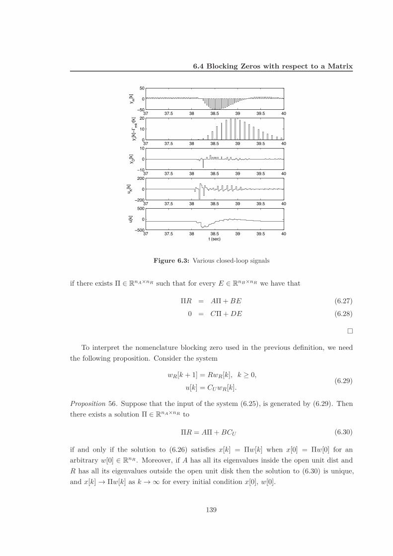
6.4 Blocking Zeros with respect to a Matrix
37 37.5 38 38.5 39 39.5 40−50
0
50
y m[k
]
37 37.5 38 38.5 39 39.5 400
10
20
y r[k]−K
mkr[k
]
37 37.5 38 38.5 39 39.5 40−10
0
10
y D[k
]
37 37.5 38 38.5 39 39.5 40−200
0
200
u K[k]
37 37.5 38 38.5 39 39.5 40−500
0
500
u[k]
t (sec)
Figure 6.3: Various closed-loop signals
if there exists ' + RnA#nR such that for every E + RnB#nR we have that
'R = A' + BE (6.27)0 = C' + DE (6.28)
"
To interpret the nomenclature blocking zero used in the previous definition, we needthe following proposition. Consider the system
wR[k + 1] = RwR[k], k " 0,
u[k] = CUwR[k].(6.29)
Proposition 56. Suppose that the input of the system (6.25), is generated by (6.29). Thenthere exists a solution ' + RnA#nR to
'R = A' + BCU (6.30)
if and only if the solution to (6.26) satisfies x[k] = 'w[k] when x[0] = 'w[0] for anarbitrary w[0] + RnR . Moreover, if A has all its eigenvalues inside the open unit dist andR has all its eigenvalues outside the open unit disk then the solution to (6.30) is unique,and x[k] - 'w[k] as k - / for every initial condition x[0], w[0].
139

6. OUTPUT REGULATION FOR MULTI-RATE SYSTEMS
"
Proof. If there exists ' such that (6.30) has a solution, then we can argue by inductionthat x[k] = 'w[k]. In fact this is valid by hypothesis for k = 0, and if it is valid for k = r,then
x[r + 1] 0 'w[r + 1] (6.31)= Ax[r] + BCUw[r] 0 'Rw[r]= (A' + BCU 0 'R)w[r] + A(x[r] 0 'w[r])= A(x[r] 0 'w[r]) (6.32)= 0.
Conversely if x[k] = 'w[k] when x[0] = 'w[0] for an arbitrary w[0] + RnR, then0 = x[1] 0 'w[1] = (A' + BCU 0 'R)w[0], which implies (6.30) since w[0] is arbitrary.
Now suppose that A has all its eigenvalues inside the open unit disk and R has all itseigenvalues outside the open unit disk, and that there exists two solutions ' and ', whichsatisfy (6.30). Let E := ' 0 '. Then ER = AE, which implies that ERk = AkE for everyk " 0 and this implies that E = 0. Moreover from (6.31), (6.32) and the stability of A weconclude that for every x[0], w[0], we have that x[k] - 'w[k] when k - /.
From Proposition 56, we can conclude that according to the Definition 55, the sys-tem (6.25) has a blocking zero with respect to R if the following hold. If the input of (6.25)is generated by (6.29) for an arbitrary matrix CR = E and the initial condition of (6.25)satisfies x[0] = 'w[0], then the output of (6.25) is identically zero. This suggests thenomenclature blocking zero with respect to the matrix R.
According to [98, Def. 3.14] the system (6.25) has a blocking zero at a complex numberz0 + C that does not belong to the spectrum of A, if
C(z0I 0 A)!1B + D = 0. (6.33)
As stated in the next proposition, in the case where R is scalar our definition coincideswith the one from [98, Def. 3.14],Proposition 57. Suppose that R = z0 + C is a complex number that does not belong to thespectrum of A. Then, the system (6.25) has a blocking zero according to the Definition 55if and only if (6.33) holds.
"
Proof. To prove su"ciency it su"ces to multiply (6.27) by C(z0I 0 A)!1 and sum theresult to (6.28). One obtains (C(z0I 0 A)!1B + D)E = 0 for every E, which implies (6.33).To prove necessity take ' = (z0I 0 A)!1BE, and see that (6.27)-(6.28) holds if (6.33)holds.
140
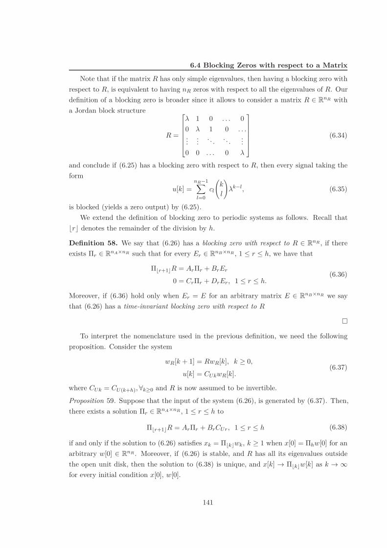
6.4 Blocking Zeros with respect to a Matrix
Note that if the matrix R has only simple eigenvalues, then having a blocking zero withrespect to R, is equivalent to having nR zeros with respect to all the eigenvalues of R. Ourdefinition of a blocking zero is broader since it allows to consider a matrix R + RnR witha Jordan block structure
R =
0
111112
" 1 0 . . . 00 " 1 0 . . .... ... . . . . . . ...0 0 . . . 0 "
3
444445(6.34)
and conclude if (6.25) has a blocking zero with respect to R, then every signal taking theform
u[k] =nR!1*
l=0cl
=k
l
>
"k!l, (6.35)
is blocked (yields a zero output) by (6.25).We extend the definition of blocking zero to periodic systems as follows. Recall that
<r= denotes the remainder of the division by h.
Definition 58. We say that (6.26) has a blocking zero with respect to R + RnR , if thereexists 'r + RnA#nR such that for every Er + RnB#nR , 1 ! r ! h, we have that
'0r+11R = Ar'r + BrEr
0 = Cr'r + DrEr, 1 ! r ! h.(6.36)
Moreover, if (6.36) hold only when Er = E for an arbitrary matrix E + RnB#nR we saythat (6.26) has a time-invariant blocking zero with respect to R
"
To interpret the nomenclature used in the previous definition, we need the followingproposition. Consider the system
wR[k + 1] = RwR[k], k " 0,
u[k] = CUkwR[k].(6.37)
where CUk = CU(k+h), 2k$0 and R is now assumed to be invertible.Proposition 59. Suppose that the input of the system (6.26), is generated by (6.37). Then,there exists a solution 'r + RnA#nR , 1 ! r ! h to
'0r+11R = Ar'r + BrCUr, 1 ! r ! h (6.38)
if and only if the solution to (6.26) satisfies xk = '0k1wk, k " 1 when x[0] = 'hw[0] for anarbitrary w[0] + RnR . Moreover, if (6.26) is stable, and R has all its eigenvalues outsidethe open unit disk, then the solution to (6.38) is unique, and x[k] - '0k1w[k] as k - /for every initial condition x[0], w[0].
141

6. OUTPUT REGULATION FOR MULTI-RATE SYSTEMS
"
Proof. If there exists 'r such that (6.38) has a solution, then we can argue by inductionthat x[k] = '0k1w[k]. In fact, this is valid by hypothesis for k = 0, and if it is valid fork = l, then
x[l + 1] 0 '0l+11w[l + 1] (6.39)= Alx[l] + BlCUlw[l] 0 '0l+11Rw[r]= (Al'0l1 + BlCUl 0 '0l+11R)w[l] + A(x[l] 0 '0l1w[l])= Al(x[l] 0 '0l1w[l]) (6.40)= 0.
Conversely if x[k] = '0k1w[k] when x[0] = 'T w[0] for an arbitrary w[0] + RnR , then0 = x[r] 0 'rw[r] = (A'r + BCU 0 'r)Rw[r] = (A'r + BCU 0 'rR)Rrw[0], whichimplies (6.30) since w[0] is arbitrary and R is invertible.
Now suppose that (6.26) is stable, R has all its eigenvalues outside the open unit disk,and that there exists two solutions 'r and 'r, which satisfy (6.30). Let Er := 'r 0 'r
for 1 ! r ! h. Then E0k1R = AkE0k1, which implies that Er = 0 for every 1 ! r ! h.Moreover from (6.39), (6.40) and the stability of (6.26) we conclude that for every x[0], w[0],we have that x[k] - '0k1w[k] when k - /.
From Proposition 59, we can conclude that according to Definition 58, the system (6.26)has a blocking zero with respect to R if the following hold. If the input of (6.26) is generatedby (6.37) for an arbitrary matrices CUk = Ek, then the output of (6.25) is identically zero.If this hold when (6.37) is time-invariant, then (6.26) with nA = nB has a time-invariantblocking zero with respect to R.
The relation between the blocking zeros of a periodic system and the blocking zeros ofits lift is provided in the next result.
Proposition 60. The periodic system (6.26) has a blocking zero with respect to R if andonly if its LTI lifted system has a blocking zero with respect to Rh.
"
Proof. From Proposition 59 we conclude that (6.26) has a blocking zero with respect toR, if and only if for every signal generated by (6.37), the output is zero. This holds if andonly if (6.43) has zero output when the input is generated by
w[l + 1] = Rhw[l]u[l] = Fw[k],
(6.41)
142

6.5 Proof of the Main Result
where
F =
0
111112
CU0CU1R
. . .
CU(h!1)Rh!1
3
444445
Since the CU&, ) + {1, . . . , h} are arbitrary and R is invertible, we see that F can be madearbitrary, and using Proposition 56 we conclude that (6.43) has a blocking zero with respectto the matrix Rh.
6.5 Proof of the Main Result
We start by reviewing some general definitions for periodically time-varying systems. Thenwe state the assumptions that we make on CI , CD that lead to establishing that there existsa system CK that yields the closed-loop of Figure 6.1 stable. After establishing the existenceof such a system CK we prove the main result. In the Appendix we introduce the notionof blocking zero with respect to a matrix, which is key to understand the assumptions onthe block CD, and to prove some of the results in the present Section.
6.5.1 Periodic Systems
Consider a discrete-time linear periodic system
R =
+,
-x[k + 1] = Akx[k] + Bku[k]
y[k] = Ckx[k] + Dku[k], k " 0,(6.42)
where x[k] + RnA , u[k] + RnB , y[k] + RnC , and Ak, Bk, Ck, Dk are h-periodic matrices,e.g., Ak = Ak+h. Many system analytical notions for (6.42) are defined by considering thelifted time-invariant system R associated with R, which is defined as
R =
+,
-x[l + 1] = Ax[l] + Bu[l]
y[l] = Cx[l] + Du[l], l " 0,(6.43)
where x[l] = x[lT ],
u[l] := (u[lh], u[lh + 1], . . . , u[lh + h 0 1]),y[l] := (y[lT ], y[lT + 1], . . . , y[lT + h 0 1]),
143

6. OUTPUT REGULATION FOR MULTI-RATE SYSTEMS
and the system matrices in (6.43) are given by A := %(h, 0),
B := [%(h, 1)B0 %(h, 2)B1 . . . Bh!1] ,
C := (C0, C1%(1, 0), . . . , Ch!1%(h 0 1, 0)),
D :=
0
112
E11 . . . E1T... ... ...
ET 1 . . . ET h
3
445 ,
Eij :=
+:::,
:::-
Ci!1%(i 0 1, j)Bj!1 i > j
Di i = j
0 i < j
,
where %(i, j) := Ai!1Ai!2 . . . Aj , for i > j and %(i, i) := I.The system R is stable, stabilizable and detectable if and only if R is stable, stabilizable
or detectable, respectively. Equivalently, stability of (6.42) is characterized by all theeigenvalues of the matrix A having norm less that one, i.e., )"i(A)) < 1, 2i, stabilizabilityof (6.42), denoted by (Ak, Bk) is stabilizable, is characterized by there exists a set ofperiodic matrices Fk, Fk = Fk+h, such that x[k + 1] = (Ak + BkFk)x[k] is stable, anddetectability of (6.42), denoted by (Ck, Ak) is detectable, is characterized by there existsa set of periodic matrices Gk, Gk = Gk+h, such that x[k + 1] = (Ak + GkCk)x[k] is stable(cf. [7]).
6.5.2 Assumptions on CI :
The system CI , described by (6.13), must be such that:
(I1) (AI , BI) is stabilizable and (CI , AI) is detectable,
(I2) CI does not have invariant zeros at the unstable eigenvalues of the plant P, i.e.,#AI 0 -InI BI
CI 0
$
is invertible (6.44)
for - + {"i(A) : )"i(A)) " 1}.
(I3) For every Z + Rm#nw , the following equation
AI'I = 'IS
CI'I = Z(6.45)
has a solution 'I + RnI#nw . Moreover such solution is unique.
(I4) The eigenvalues of AI belong to the set of eigenvalues of S.
144

6.5 Proof of the Main Result
We assume (I1)-(I2) to obtain (G1). The assumption (I4) is required to limit the setof possible systems CI . As stated in the next proposition the assumption (I3) is closelyrelated to the purpose of the system CI , i.e., to provide the adequate input to the plant sothat it tracks the reference signal. Note that due to the linearity of the plant, an adequateinput takes the same form of the reference signal one wishes to follow, i.e., it is generatedby
w[k + 1] = Sw[k], k " 0,
u[k] = CUw[k]. (6.46)
Proposition 61. If (I3) holds then for any signal u[k] generated by (6.46) there exists aninitial condition x0 such that the free motion of
xI [k + 1] = AIxI [k], xI [0] = x0
yI [k] = CIxI [k]
is such that yI [k] = u[k].
"
Proof. (of proposition 61) If (I3) holds then for an initial condition xI [0] = 'Iw[0], wehave that
yI [k] = CIAkI 'Iw[0] = CI'ISkw[0] = ZSkw[0].
The result follows by making Z = CU .
Due to the following proposition it is always possible to find BJ and CJ such that(I1)-(I3) hold for the system (6.13) with matrices (6.14).
Proposition 62. The set of matrices (BJ , CJ) + Rnw#1 # R1#nw for which (I1)-(I3) do nothold for the system (6.13) with matrices (6.14) is a set of measure zero in Rnw#1 # R1#nw .
"
Proof. Since the union of sets of measure zero has measure zero it su"ces to prove thatfor each assumption (I1), (I2), and (I3) the set of matrices (BJ , CJ ) + Rnw#1 # R1#nw
which do not satisfy each of these assumption has measure zero. We start by showing thisfor (I1). If (S, BJ) is not stabilizable, there exists a left eigenvalue of S, say wi, for some1 ! i ! ns, such that w!
i BJ = 0. Since the set {BJ : w!i BJ = 0, for every 1 ! i ! ns}
where (S, BJ ) is not stabilizable has measure zero, we establish that (S, BJ ) is stabilizableexcept in a set of measure zero in BJ + Rnw#1. A similar reasoning allows to conclude that(CJ , S) is detectable except in a set of measure zero in CJ + R1#nw . Since stabilizabilityof (S, BJ) implies that of (AI , BI) and detectability of (CJ , S) implies that of (CI , AI), we
145
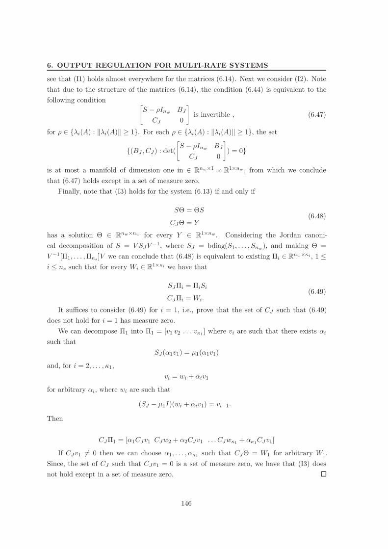
6. OUTPUT REGULATION FOR MULTI-RATE SYSTEMS
see that (I1) holds almost everywhere for the matrices (6.14). Next we consider (I2). Notethat due to the structure of the matrices (6.14), the condition (6.44) is equivalent to thefollowing condition #
S 0 -Inw BJ
CJ 0
$
is invertible , (6.47)
for - + {"i(A) : )"i(A)) " 1}. For each - + {"i(A) : )"i(A)) " 1}, the set
{(BJ , CJ) : det(#S 0 -Inw BJ
CJ 0
$
) = 0}
is at most a manifold of dimension one in + Rnw#1 # R1#nw , from which we concludethat (6.47) holds except in a set of measure zero.
Finally, note that (I3) holds for the system (6.13) if and only if
S# = #S
CJ# = Y(6.48)
has a solution # + Rnw#nw for every Y + R1#nw . Considering the Jordan canoni-cal decomposition of S = V SJV !1, where SJ = bdiag(S1, . . . , Snw), and making # =V !1['1, . . . , 'ns ]V we can conclude that (6.48) is equivalent to existing 'i + Rnw#&i , 1 !i ! ns such that for every Wi + R1#&i we have that
SJ'i = 'iSi
CJ'i = Wi.(6.49)
It su"ces to consider (6.49) for i = 1, i.e., prove that the set of CJ such that (6.49)does not hold for i = 1 has measure zero.
We can decompose '1 into '1 = [v1 v2 . . . v&1] where vi are such that there exists $i
such thatSJ($1v1) = µ1($1v1)
and, for i = 2, . . . , )1,vi = wi + $iv1
for arbitrary $i, where wi are such that
(SJ 0 µ1I)(wi + $iv1) = vi!1.
Then
CJ'1 = [$1CJv1 CJw2 + $2CJv1 . . . CJw&1 + $&1CJv1]
If CJv1 1= 0 then we can choose $1, . . . , $&1 such that CJ# = W1 for arbitrary W1.Since, the set of CJ such that CJv1 = 0 is a set of measure zero, we have that (I3) doesnot hold except in a set of measure zero.
146
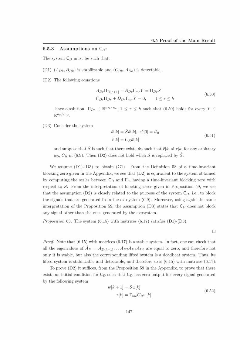
6.5 Proof of the Main Result
6.5.3 Assumptions on CD:
The system CD must be such that:
(D1) (ADk, BDk) is stabilizable and (CDk, ADk) is detectable.
(D2) The following equations
ADr'D0r+11 + BDr(mrY = 'DrS
CDr'Dr + DDr(mrY = 0, 1 ! r ! h(6.50)
have a solution 'Dr + RnD#nw , 1 ! r ! h such that (6.50) holds for every Y +Rnm#nw .
(D3) Consider the systemw[k] = Sw[k], w[0] = w0
r[k] = CRw[k](6.51)
and suppose that S is such that there exists w0 such that r[k] 1= r[k] for any arbitraryw0, CR in (6.9). Then (D2) does not hold when S is replaced by S.
We assume (D1)-(D3) to obtain (G1). From the Definition 58 of a time-invariantblocking zero given in the Appendix, we see that (D2) is equivalent to the system obtainedby computing the series between CD and (m having a time-invariant blocking zero withrespect to S. From the interpretation of blocking zeros given in Proposition 59, we seethat the assumption (D2) is closely related to the purpose of the system CD, i.e., to blockthe signals that are generated from the exosystem (6.9). Moreover, using again the sameinterpretation of the Proposition 59, the assumption (D3) states that CD does not blockany signal other than the ones generated by the exosystem.
Proposition 63. The system (6.15) with matrices (6.17) satisfies (D1)-(D3).
"
Proof. Note that (6.15) with matrices (6.17) is a stable system. In fact, one can check thatall the eigenvalues of AD = AD(h!1) . . . AD2AD1AD0 are equal to zero, and therefore notonly it is stable, but also the corresponding lifted system is a deadbeat system. Thus, itslifted system is stabilizable and detectable, and therefore so is (6.15) with matrices (6.17).
To prove (D2) it su"ces, from the Proposition 59 in the Appendix, to prove that thereexists an initial condition for CD such that CD has zero output for every signal generatedby the following system
w[k + 1] = Sw[k]r[k] = (mkCRw[k]
(6.52)
147
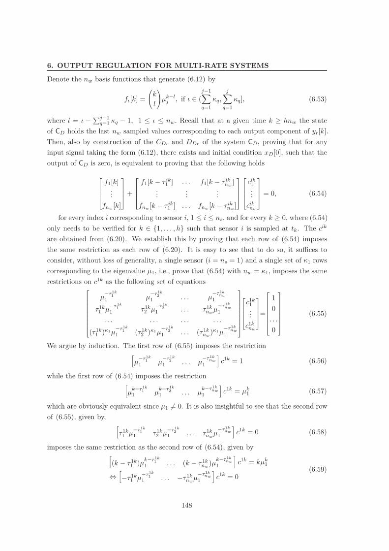
6. OUTPUT REGULATION FOR MULTI-RATE SYSTEMS
Denote the nw basis functions that generate (6.12) by
f)[k] ==
k
l
>
µk!lj , if 0 + (
j!1*
q=1)q,
j*
q=1)q], (6.53)
where l = 0 0!j!1
q=1 )q 0 1, 1 ! 0 ! nw. Recall that at a given time k " hnw the stateof CD holds the last nw sampled values corresponding to each output component of yr[k].Then, also by construction of the CDr and DDr of the system CD, proving that for anyinput signal taking the form (6.12), there exists and initial condition xD[0], such that theoutput of CD is zero, is equivalent to proving that the following holds
0
112
f1[k]...
fnw [k]
3
445 +
0
112
f1[k 0 ! ik1 ] . . . f1[k 0 ! ik
nw]
... ... ...fnw [k 0 ! ik
1 ] . . . fnw [k 0 ! iknw
]
3
445
0
112
cik1...
ciknw
3
445 = 0, (6.54)
for every index i corresponding to sensor i, 1 ! i ! ns, and for every k " 0, where (6.54)only needs to be verified for k + {1, . . . , h} such that sensor i is sampled at tk. The cik
are obtained from (6.20). We establish this by proving that each row of (6.54) imposesthe same restriction as each row of (6.20). It is easy to see that to do so, it su"ces toconsider, without loss of generality, a single sensor (i = ns = 1) and a single set of )1 rowscorresponding to the eigenvalue µ1, i.e., prove that (6.54) with nw = )1, imposes the samerestrictions on c1k as the following set of equations
0
1111112
µ!*1k
11 µ
!*1k2
1 . . . µ!*1k
nw1
!1k1 µ
!*1k1
1 !1k2 µ
!*1k2
1 . . . !1knw
µ!*1k
nw1
. . . . . . . . . . . .
(!1k1 )&1µ
!*1k1
1 (!1k2 )&1µ
!*1k2
1 . . . (!1knw
)&1µ!*1k
nw1
3
4444445
0
112
c1k1...
c1knw
3
445=
0
111112
10
. . .
0
3
444445(6.55)
We argue by induction. The first row of (6.55) imposes the restriction%µ
!*1k1
1 µ!*1k
21 . . . µ
!*1knw
1
&c1k = 1 (6.56)
while the first row of (6.54) imposes the restriction%µ
k!*1k1
1 µk!*1k
21 . . . µ
k!*1knw
1
&c1k = µk
1 (6.57)
which are obviously equivalent since µ1 1= 0. It is also insightful to see that the second rowof (6.55), given by,
%!1k
1 µ!*1k
11 !1k
2 µ!*1k
21 . . . !1k
nwµ
!*1knw
1
&c1k = 0 (6.58)
imposes the same restriction as the second row of (6.54), given by%(k 0 !1k
1 )µk!*1k1
1 . . . (k 0 !1knw
)µk!*1knw
1
&c1k = kµk
1
6%0!1k
1 µ!*1k
11 . . . 0!1k
nwµ
!*1knw
1
&c1k = 0
(6.59)
148

6.5 Proof of the Main Result
where we used (6.56).Now assuming that the first 1 ! r 0 1 < nw 0 1 rows of (6.54) impose the same
restriction as the first 1 ! r 0 1 < nw 0 1 rows (6.55), we prove that the same is true forthe row r, i.e.,
%fr[k 0 !1k
1 ] fr[k 0 !1k2 ] . . . fr[k 0 !1k
nw]&
c1k = fr[k] (6.60)
To this e!ect, note that we can write (6.53) as
fr[k 0 ! ] ==
k 0 !
r
>
µk!r!*1
= (r*
m=0amk(r!m)!m)µk!r!*
1
= (r!1*
m=0amk(r!m)!m + ar! r)µk!r!*
1 (6.61)
for some coe"cients am implicitly defined from=
k 0 !
r
>
= (k 0 !)(k 0 ! 0 1) . . . (k 0 ! 0 r)
=r*
m=0amk(r!m)!m.
Note that ar = (01)r+1. If we replace (6.61) in (6.60) and use the fact that the first r 0 1restrictions of (6.55) hold, we obtain
ar
%(!1k
1 )rµk!r!*1k
1j . . . (!1k
nw)rµ
k!r!*1knw
j
&c1
k = 0
which is equivalent to the restriction associated with row r of (6.55) since µ1 1= 0 andar 1= 0.
To prove that (6.15) with matrices (6.17) satisfies (D3), note that using the interpre-tation of a blocking zero given in the Proposition 59, the assumption (D3) states that CD
does not block any other signal other than the ones generated by the exosystem. To seethat this is true, suppose that there exists a signal g[k] such that there exists an initialcondition to the system CD such that the output of the system CD is identically zero wheng[k] is applied to its input. Then, by construction of CD, i.e., by the fact that for k " nwh,xD[k] will hold the value of the last nw samples of every sensor 1 ! i ! ns, g[k] mustsatisfy
g[k] +%g[k 0 ! ik
1 ] g[k 0 ! ik2 ] . . . g[k 0 ! ik
nw]&
cik = 0
for every, 1 ! i ! ns and k + {1, . . . , h} such that sensor i is sampled at tk. From (6.54) anduniqueness of the cik(cf. (6.19), (6.20)) we conclude that g[k] must be a linear combinationof the f)[k], 1 ! 0 ! nw and therefore g[k] can be generated by the exosystem.
149
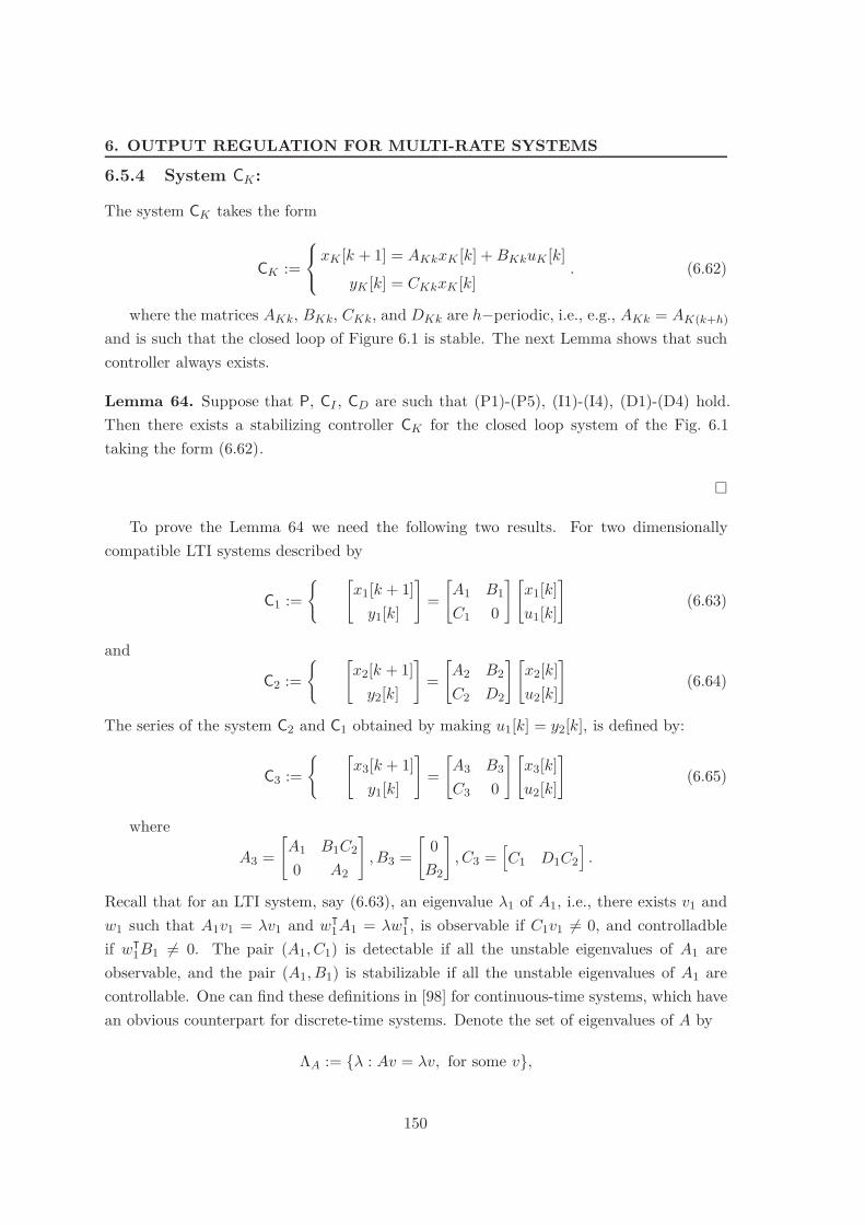
6. OUTPUT REGULATION FOR MULTI-RATE SYSTEMS
6.5.4 System CK:
The system CK takes the form
CK :=
+,
-xK [k + 1] = AKkxK [k] + BKkuK [k]
yK [k] = CKkxK [k]. (6.62)
where the matrices AKk, BKk, CKk, and DKk are h0periodic, i.e., e.g., AKk = AK(k+h)and is such that the closed loop of Figure 6.1 is stable. The next Lemma shows that suchcontroller always exists.
Lemma 64. Suppose that P, CI , CD are such that (P1)-(P5), (I1)-(I4), (D1)-(D4) hold.Then there exists a stabilizing controller CK for the closed loop system of the Fig. 6.1taking the form (6.62).
"
To prove the Lemma 64 we need the following two results. For two dimensionallycompatible LTI systems described by
C1 :=< #
x1[k + 1]y1[k]
$
=#A1 B1C1 0
$ #x1[k]u1[k]
$
(6.63)
and
C2 :=< #
x2[k + 1]y2[k]
$
=#A2 B2C2 D2
$ #x2[k]u2[k]
$
(6.64)
The series of the system C2 and C1 obtained by making u1[k] = y2[k], is defined by:
C3 :=< #
x3[k + 1]y1[k]
$
=#A3 B3C3 0
$ #x3[k]u2[k]
$
(6.65)
where
A3 =#A1 B1C20 A2
$
, B3 =#
0B2
$
, C3 =%C1 D1C2
&.
Recall that for an LTI system, say (6.63), an eigenvalue "1 of A1, i.e., there exists v1 andw1 such that A1v1 = "v1 and w!
1A1 = "w!1 , is observable if C1v1 1= 0, and controlladble
if w!1B1 1= 0. The pair (A1, C1) is detectable if all the unstable eigenvalues of A1 are
observable, and the pair (A1, B1) is stabilizable if all the unstable eigenvalues of A1 arecontrollable. One can find these definitions in [98] for continuous-time systems, which havean obvious counterpart for discrete-time systems. Denote the set of eigenvalues of A by
&A := {" : Av = "v, for some v},
150

6.5 Proof of the Main Result
where A can be replaced by A1, A2, A3. Also denote the set of eigenvalues of A which arenot eigenvalues of B by
&A/B := {" : " + &A and " /+ &B},
where A, B can be replace by A1 and A2.
Proposition 65. Consider C1, C2 and the series C3. Then
(i) &A3 = &A1 : &A2
(ii) If " + &A1/A2 then " is an observable eigenvalue of C3 if " is an observable eigenvalueof C1.
(iii) If " + &A2 then " is an observable eigenvalue of C3 if " is an observable eigenvalueof C2 and C1 has no invariant zeros at ".
(iv) If " + &A2/A1 then " is a controllable eigenvalue of C3 if " is a controllable eigenvalueof C2.
(v) If " + &A1 then " is a controllable eigenvalue of C3 if " is a controllable eigenvalueof C1 and C2 has no invariant zeros at ".
"
Proof. (i) We can conclude from det("I 0 A3) = det("I 0 A1) det("I 0 A2), which holdsdue to the structure of A3.We prove only (ii) and (iii) since (iv) and (v) can be obtained from the fact that detectabilityand stabilizability are dual notions. To this e!ect consider the following equation for theeigenvalues of A3 #
A1 B1C20 A2
$ #v1v2
$
= "
#v1v2
$
If " + &A1/A2 then v1 : A1v1 = "v1 and v2 = 0. Thus C3[v!1 v!2 ]! = C1v1 1= 0, which meansthat " is an observable eigenvalue of C3 if it is an observable eigenvalue of C1, which is (ii).
If " + &A2 then v2 : A2v2 = "v2 and v1 : A1v1 +B1v2 = "v1. If " was not an observableeigenvalue of C3 then we would have C3[v!1 v!2 ]! = 0 which would imply that
#A1 0 "1I B1
C1 D1
$ #v1
C2v2
$
= 0 (6.66)
where C2v2 1= 0 since " is an observable eigenvalue of C2. The equation (6.66) contradictsthe assumption that C1 has no invariant zeros at ".
151

6. OUTPUT REGULATION FOR MULTI-RATE SYSTEMS
The series of two periodically time-varying systems is defined similarly to the series oftwo LTI systems.
Proposition 66. The lift of the series of two periodic systems is the series of the LTI liftsystems of each periodic system.
"
Proof. Obtained by direct replacement.
We shall need the following proposition.
Proposition 67. Consider the system
x[k + 1] = Ax[k]y[k] = bdiag(.1
k , . . . , .ny
k )Cx[k](6.67)
where y[k] + Rny . The .ik + {0, 1}, 1 ! i ! ny are h0 periodic, i.e., .i
k = .ik+h, and for
each i are equal to 1 at least once in a period. The (6.67) is detectable if and only if thepair (A, C) is detectable.
"
Proof. See [18]
We shall also need to take into account that if we apply the lift for an LTI system weobtain the following eigenvalues of the lifted system.
&Ah := {"h, " + &A} (6.68)
The Lemma 64 is proved next.
Proof. In [16], it is shown that a periodic system R taking the form (6.42) is detectable andstabilizable if and only if there exists a periodic linear controller, taking the form (6.62)such that the closed loop system is asymptotically stable. Thus it su"ces to prove thestabilizability and detectability of the periodic system obtained by computing the seriesof CI , P, and CD, which is a periodic system that we shall term CA. This can proved byestablishing stabilizability and detectability of the lifted LTI system, denoted by CA. FromProposition 66 the lift of CA is the series of the lift of each individual system CI , P, andCD, which are denoted by CI , P, and CD, respectively. Thus, we only have to prove theobservability and controllability of the unstable eigenvalues of CA, corresponding to theunstable eigenvalues of CI and P, since CD is a deadbeat system and thus stable.
We start by establishing stabilizability. From Proposition 65(iv) the controllabilityof the unstable eigenvalues of CA associated with P or with CI , do not depend of CD
152
6.5 Proof of the Main Result
(which has only stable eigenvalues), and since CI , P are LTI systems, this amounts toan LTI test. In fact, for an LTI system, considered to be a special case of a periodicsystem with period h, stabilizability of the lift is equivalent to stabilizability of the originalLTI system, which can be concluded from the definition of stabilizability for periodicsystems. Thus, it su"ces to prove that the LTI series of CI , P, which we denote by CIP , isstabilizable. The eigenvalues of CIP belonging to &CI/CP
are controllable due to (I1) andProposition 65(iv). The eigenvalues of CIP belonging to &CP are controllable due to (P1),(I2), and Proposition 65(v).
We prove next detectability. To prove that observability of the unstable eigenvalues ofCA belonging to &CI
, which in turn correspond to unstable eigenvalues of CI , due to (6.68),it su"ces to prove that these eigenvalues are detectable from the plant output yr[k], i.e.,if we consider the system obtained by the series of CI and Pr where Pr is the systemobtained by considering the plant with yr[k] has the only output. Again this amounts toan LTI test, since the series of CI and Pr is an LTI system with multi-rate measurementsas in Proposition 67, where we state that for such system detectability can be proved byan LTI test. The desired conclusion follows then from Assumptions (I1), (I4), (P2), andProposition 65(iii).
To see the observability of the unstable eigenvalues of CA that correspond to those of Pit su"ces to consider those not observable through yr[k]. By this we mean, the eigenvaluesof the plant P that are not an observable eigenvalue of the pair (A, Cr). The existence ofsuch eigenvalue, is equivalent to existing an initial condition for the plant x[0] such that
x[k + 1] = Ax[k]yr[k] = (rCrx[k]
(6.69)
has zero output, i.e., yr[k] = 0, 2k$0. From assumption (P3) there cannot exist an initialcondition for the plant such that (6.69) has a zero output yr[k] = 0 and ym[k] can begenerated by the exosystem. Since by assumption (D3), the system CD does not cancelsignals other than those generated by the exosystem, we obtain that this yields a non-zerooutput for CD and thus these eigenvalues of A are also observable for the system CA.
6.5.5 Output Regulation
The following result and Lemma 64 allows to conclude the main result of the chapter, i.e.,Theorem 53.
Theorem 68. Suppose that (P1)-(P3) hold for the plant P. Then one can find CI suchthat (I1)-(I4) holds, CD such that (D1)-(D4) hold, and CK such that the closed-loop inFigure 6.1 is stable. Moreover, output regulation is achieved even in the presence of plantuncertainties that do not destroy closed-loop stability.
153

6. OUTPUT REGULATION FOR MULTI-RATE SYSTEMS
"
Proof. The first part of the Theorem has been established in Proposition 62 and 63 andLemma 64. Thus, it su"ces to prove that output regulation is achieved. We start bywriting the equations for the series connection of CI , P, and CD, which are given by
xA[k + 1] = AAkxA[k] + BAkuA[k] + BAwkw[k]yA[k] = CAkxA[k] + DAwkw[k]
where
AAk =
0
112
A BCI 00 AI 0
BDk(mkCm 0 ADk
3
445
BAk =
0
112
0BI
0
3
445
CAk =#DDk(mkCm 0 CDk
(rkCr 0 0
$
BAwk =
0
112
BV CV
00
3
445
DAwk =#
00(rkCR
$
Let CK be a stabilizing controller described by (6.62), whose existence is established inLemma 64. Then the closed-loop is described by
#xA[k + 1]xK [k + 1]
$
=#
AAk BAkCDk
BKkCAk AKk
$#xA[k]xK [k]
$
+#
BAwk
BKkDAwk
$
w[k]. (6.70)
where w[k] is described by (6.9). Using the fact that the periodic system (6.70) is stable,since CK is a stabilizing controller, from Proposition 59 in the Appendix, we conclude thatthere exists unique 'k, k + {1, . . . h}, such that
#AAk BAkCKk
BKkCAk AKk
$
'k +#
BAwk
BKkDAwk
$
= '0k+11S (6.71)
and for any initial condition (xA[0], xK [0]) the state of the system tends asymptotically to#
xA[k]xK [k]
$
= 'kw[k] (6.72)
154
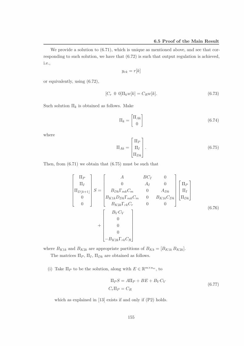
6.5 Proof of the Main Result
We provide a solution to (6.71), which is unique as mentioned above, and see that cor-responding to such solution, we have that (6.72) is such that output regulation is achieved,i.e.,
yrk = r[k]
or equivalently, using (6.72),
[Cr 0 0]'kw[k] = CRw[k]. (6.73)
Such solution 'k is obtained as follows. Make
'k =#'Ak
0
$
(6.74)
where
'Ak =
0
112
'P
'I
'Dk
3
445 . (6.75)
Then, from (6.71) we obtain that (6.75) must be such that
0
11111112
'P
'I
'D0k+11
00
3
44444445
S =
0
11111112
A BCI 00 AI 0
BDk(mkCm 0 ADk
BK1kDDk(mkCm 0 BK1kCDk
BK2k(rkCr 0 0
3
44444445
0
112
'P
'I
'Dk
3
445
+
0
11111112
BV CV
000
0BK2k(rkCR
3
44444445
(6.76)
where BK1k and BK2k are appropriate partitions of BKk = [BK1k BK2k].The matrices 'P , 'I , 'Dk are obtained as follows.
(i) Take 'P to be the solution, along with E + Rm#nw , to
'P S = A'P + BE + BV CV
Cr'P = CR
(6.77)
which as explained in [13] exists if and only if (P2) holds.
155

6. OUTPUT REGULATION FOR MULTI-RATE SYSTEMS
(ii) Take 'I to be the unique solution to
AI'I = 'IS
CI'I = E
where E is, along with 'P , the solution to (6.77). Note that such solution 'I existsdue to the Assumption (I3).
(iii) Take 'Dk to be the solution to
ADk'Dk + BDk(mkCm'P = 'D0k+11S
CDk'Dk + DDk(mkCm'P = 0(6.78)
which exists due to the Assumption (D3) and is unique due to Proposition 59 andthe fact that CD is a stable system.
By construction, we conclude that 'k given by (6.74), where 'Ak is given by (6.75), and'P , 'I and 'Dk are described by (i), (ii) and (iii), respectively, satisfies (6.71) and (6.73)and therefore output regulation is achieved.
Note that in the proof we only required the controller CK to stabilize the closed-loop.If the plant describing matrices are not known but CK still stabilizes the closed-loop theproof remains unchanged.
Proof. (of Theorem 53) Follows as a Corollary of Lemma 64 and Theorem 68, provided thatwe notice that the matrices BJ and CJ can be chosen such that CI , given by (6.13), satisfies(I1)-(I4) (cf.Proposition 62) and that we notice that CD, given by (6.16), (6.17), (6.18)satisfies (D1)-(D3) (cf.Proposition (63)).
6.6 Further Comments and References
Several solutions were proposed in the seventies using di!erent approaches (see, e.g., [26],[95], [33], [34]), and all incorporate an internal model of the exosystem, as well as a con-troller that stabilizes the closed loop. The necessity of incorporating a model of the ex-osystem in the controller was proved in [34], and is thereafter known as the internal modelprinciple.
The blossom of the research in multi-rate systems took place in the early nineties,where many standard problems for LTI systems have been extended to multi-rate systems.For example, structural properties for multi-rate systems including stabilizability and de-tectability notions are provided in [65], a solution to the output pole placement problemcan be found in [18], and the linear quadratic gaussian problem for multi-rate systems issolved in [20]. The close relation between multi-rate and periodic systems (see, e.g., [9]),
156
6.6 Further Comments and References
entails that these definitions and problem solutions are often based on the concept of lifting(see [68]), i.e., considering the LTI system obtained by writing the equations of the periodicsystem along a period.
The output regulation problem for multi-rate systems was addressed in [82]. Seealso [19] for the special case where the exogenous references are constant signals. How-ever, both in [82] and [19] the analysis is restricted to square systems, i.e., systems withthe same number of inputs and measured outputs, which are also the outputs to be reg-ulated. The solution in [82] and [19] consists of designing a stabilizing controller for thesystem obtained by adding an internal model of the exosystem in series with the inputof the plant. The peculiarities of the multi-rate systems that prevented the authors fromgeneralizing the solution to non-square systems, are discussed in [82].
The present chapter may be viewed as a follow up work of [ASC08a], and [ASC10],where the output regulation problem was considered for non-square multi-rate systems inthe special case where the exogenous reference signals are constant signals. For constantreference signals, the proposed controller structure, is shown in [ASC08a], and [ASC10]not only to be suited for output regulation but also that it can be exploited to implementnonlinear gain-scheduled controllers in such a way that a fundamental property known aslinearization property is satisfied.
157
6. OUTPUT REGULATION FOR MULTI-RATE SYSTEMS
158

7
Gain-Scheduled Controllers forMulti-Rate Systems
In this chapter we present a new methodology for the design and implementation of gain-scheduled controllers for multi-rate systems.
The standard procedure for designing a gain-schedulling controller involves the followingsteps (cf. [81]): (i) the selection of scheduling variables or parameters; (ii) linearization ofthe non-linear plant about the equilibrium manifold; (iii) synthesis of controllers for thefamily of plant linearizations, which typically involves linear controller design for a givenset of equilibrium points; and (iv) implementation of the controller.
Since the controllers are designed for time-frozen parameters and when implementedthe parameters are allowed to vary, the linearization of the nonlinear gain-scheduled con-troller about a given equilibrium point does not in general match the designed time-frozenlinear controller. This mismatch is commonly known as the hidden coupling [81] and mightlead to performance degradation or even instability. Therefore, for a correct implementa-tion of the controllers, the following property is required to hold:
Linearization property: At each equilibrium point, the nonlinear gain-scheduled controllermust linearize to the linear controller designed for that equilibrium.
A technique known as the velocity implementation, presented in [51], [52] and discussedin [53], [81] which is related with the work presented herein, provides a simple solutionfor the implementation of controllers with integral action that satisfies the linearizationproperty.
Our proposed implementation satisfies the linearization property and boils down tothe velocity implementation for single-rate systems. The key to our solution is a regulatorstructure which can be obtained with the tools developed in the previous Chapter. Building
159

7. GAIN-SCHEDULED CONTROLLERS FOR MULTI-RATE SYSTEMS
upon the work presented in [81] for the continuous time case, and in [62, 63] for the single-rate sampled-data case, we guarantee i) local stability of the feedback interconnection of thesampled-data multi-rate system and gain-scheduled controller about individual equilibria,and ii) ultimate boundedness of a conveniently defined closed-loop error in response toslowly varying exogenous inputs.
We illustrate the applicability of our results in the problem of steering an autonomousrotorcraft along a predefined trajectory. Simulation results obtained with a full non-linearrotorcraft dynamic model are presented and discussed.
The remainder of the Chapter is organized as follows. Section 7.1 describes the problemformulation and Sections 7.2 and 7.3 present the main results. In Section 7.4 we apply theproposed methodology to the design of an integrated guidance and control system thataddresses the trajectory tracking problem for a small-scale rotorcraft, and evaluate theperformance of the resulting nonlinear feedback system in simulation. Section 7.5 givesfurther comments and references.
7.1 Problem Formulation
Consider the nonlinear system
G :=
+,
-x(t) = f(x(t), u(t), w(t))y(t) = h(x(t), w(t))
(7.1)
where f and h are twice continuously di!erentiable functions, x(t) + Rn is the state, u(t) +Rm is the control input, and the vector w(t) + Rnw contains references and possibly otherexogenous inputs. The vector y(t) + Rp can be decomposed as y(t) = [ym(t)T yr(t)T ]T =[hm(x(t), w(t))T hr(x(t), w(t))T ]T where ym(t) + Rnym is a vector of measured outputsavailable for feedback and yr(t) + Rnyr is a vector of tracking outputs, which we assumeto have the same dimensions as the control input, nyr = m. This vector is requiredto track the reference r(t) with zero steady state error, i.e., the error vector defined ase(t) := yr(t) 0 r(t) must satisfy e(t) = 0 at steady-state. Some of the components of yr(t)may be included in ym(t) as well.
7.1.1 Linearization Family
We assume that there exists a unique family of equilibrium points for G of the form
* :={(x0, u0, w0) : f(x0, u0, w0)=0, yr0 =hr(x0, w0)=r0}
which can be parameterized by a vector $0 + + + Rs, s.t.
* = {(x0, u0, w0) = a($0), $0 + +} (7.2)
160

7.1 Problem Formulation
where a is a continuously di!erentiable function. We further assume that there exists acontinuously di!erentiable function v such that $0 = v(y0, w0). By applying the functionv to the measured values of y and w, we obtain the variable
$ = v(y, w), (7.3)
which is usually referred to as the scheduling variable.Linearizing the nonlinear system G about the equilibrium manifold * parameterized
by $0 yields the family of linear systems
Gl($0) :=#x'(t)y'(t)
$
=#
A($0) B1($0) B2($0)C2($0) D21($0) 0
$0
112
x'(t)w'(t)u'(t)
3
445 (7.4)
where, e.g. A($0) = ,f,x(a($0)) and x'(t) = x(t) 0 x0.
7.1.2 Multi-Rate Sensors and Actuators
We consider that the sample and hold devices that interface the discrete-time controllerand the continuous-time plant operate at di!erent rates. Associated with each sampler Si,corresponding to the ith component of y(t), there is a sequence of sampling times {,i
1, ,i2, ..}
that verify 0 < ,ij < ,i
j+1. Similarly, associated with each holder Hi, correspondingto the ith component of u(t), there is a sequence of hold times {! i
1, ! i2, ..} that verify
0 < ! ij < ! i
j+1. We assume that the sample and hold operations are periodic and thattheir periods are related by rational numbers. Thus we can define a sequence of equallyspaced time instants {t0, t1, ...}, tk+1 0 tk = ts, k + Z+, such that for every samplingtime ,i
j and hold time ! ij there exists a k1 and a k2 for which ,i
j = tk1 and ! ij = tk2. In
addition, we introduce the matrix (k = diag(g1(k), ..., gp(k)), where gi(k) = 1 if ,ij =
tk for some j and gi(k) = 0 otherwise, and the matrix )k := diag(r1(k), ..., rm(k)), whereri(k) = 1 if ! i
j = tk for some j and ri(k) = 0 otherwise. Due to the periodic nature ofthe sample and hold devices we have (k = (k+h and )k = )k+h, for some positive integerh which denotes the period. We further assume that every output is sampled and everyinput is updated at least once in a period.
The multi-rate sample and hold operators can then be written as
S : L(R+) ,- l(Z+) H : l(Z+) ,- L(R+)S = (dSts H = Hts)d
(7.5)
where the operators )d : l(Z+) ,- l(Z+), Hts : l(Z+) ,- L(R+), Sts : L(R+) ,- l(Z+) and(d : l(Z+) ,- l(Z+) are given by
)d :*k+1 = (I 0 )k)*k + )kuk, *0 = 0uk = (I 0 )k)*k + )kuk
Hts :u(t)= uk
t +[tk, tk+1[
161

7. GAIN-SCHEDULED CONTROLLERS FOR MULTI-RATE SYSTEMS
Sts :yk =#ymk
yrk
$
= y(tk) (d :yk =#(mk 0
0 (rk
$ #ymk
yrk
$
and (k =#(mk 0
0 (rk
$
is partitioned according to the output decomposition yT = [yTm yT
r ].
Similarly to y(t), the values of r(t) sampled at the instants tk are denoted by rk and totake into account the multi-rate nature of the outputs we define rk = (rk rk. We can thenintroduce the error variables ek = yrk 0 rk and ek = yrk 0 rk.
7.1.3 Problem Statement
Given this setup the problem addressed in this paper can be stated as follows:Problem 69. 1) For a fixed operating point $0, find a possibly time-varying discrete-timelinear controller C($0) : [y%mk, ek] ,- u%k
C($0)=
+::,
::-
#xc
'k+1
u'k
$
=#Ac
k($0) Bc1k($0) Bc
2k($0)Cc
k($0) Dc1k($0) Dc
2k($0)
$0
112
xc'k
y'mk
ek
3
445 (7.6)
for the linearization of the nonlinear plant (7.4) with multi-rate interface (7.5) that stabi-lizes the closed loop system and achieves zero steady-state error for ek, where u'k = uk 0u0,y'mk = ymk 0 (mkym0, and ym0 =hm(x0, w0).2) Based on the family of linear controllers C($0), implement a discrete-time controller K,possibly nonlinear and time-varying, that verifies the linearization property, which will bedefined shortly, and takes the form
K =
+,
-xc
k+1 = fc(xck, ymk, ek, $k, k)
uk = hc(xck, ymk, ek, $k, k)
, (7.7)
where xck + RnK and given its dependence on the scheduling variable $k sampled at time
tk, K is referred to as a gain-scheduled controller. By linearization property we formallymean that if we consider a family of equilibrium points *c for the controller compatiblewith the family of equilibrium points * defined in (7.2), such that
*c :={xc0 : xc
0 =fc(xc0, ym0, 0, $0, k), u0 =hc(xc
0, ym0, 0, $0, k),(x0, u0, w0) = a($0), $0 + +}
the controller K linearizes to C($0), at each equilibrium point $0, that is, for example,,fc,xc ($0, k) = Ac
k($0) and ,hc,ym
($0, k) = Dc1k($0).
The proposed solution for part 2) has an a gain-scheduled structure and we will showthat under mild assumptions the linearization property just described is su"cient to guar-antee local stability about each equilibrium point of the feedback interconnection of thenon-linear plant and a gain-scheduled controller with multi-rate interface.
162
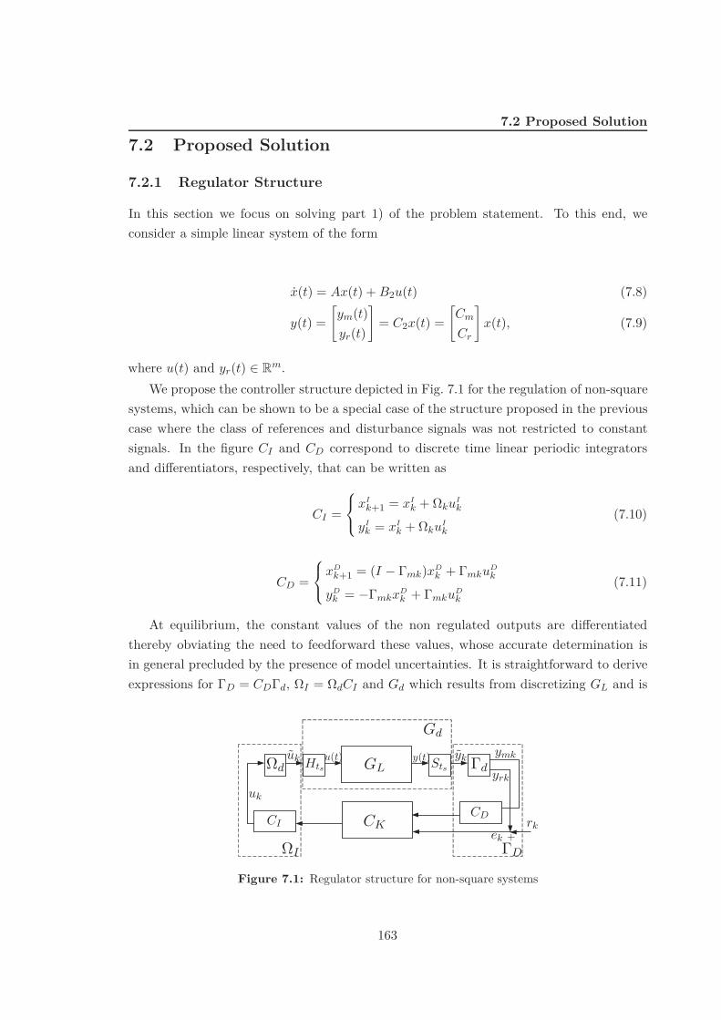
7.2 Proposed Solution
7.2 Proposed Solution
7.2.1 Regulator Structure
In this section we focus on solving part 1) of the problem statement. To this end, weconsider a simple linear system of the form
x(t) = Ax(t) + B2u(t) (7.8)
y(t) =#ym(t)yr(t)
$
= C2x(t) =#Cm
Cr
$
x(t), (7.9)
where u(t) and yr(t) + Rm.We propose the controller structure depicted in Fig. 7.1 for the regulation of non-square
systems, which can be shown to be a special case of the structure proposed in the previouscase where the class of references and disturbance signals was not restricted to constantsignals. In the figure CI and CD correspond to discrete time linear periodic integratorsand di!erentiators, respectively, that can be written as
CI =
+,
-xI
k+1 = xIk + )kuI
k
yIk = xI
k + )kuIk
(7.10)
CD =
+,
-xD
k+1 = (I 0 (mk)xDk + (mkuD
k
yDk = 0(mkxD
k + (mkuDk
(7.11)
At equilibrium, the constant values of the non regulated outputs are di!erentiatedthereby obviating the need to feedforward these values, whose accurate determination isin general precluded by the presence of model uncertainties. It is straightforward to deriveexpressions for (D = CD(d, )I = )dCI and Gd which results from discretizing GL and is
GL
ymk
yrk
y(t) yk
rkek
uk
u(t)uk
+
StsHts
CICDCK
)d
)I (D
(d
Gd
Figure 7.1: Regulator structure for non-square systems
163

7. GAIN-SCHEDULED CONTROLLERS FOR MULTI-RATE SYSTEMS
given by
Gd =
+::,
::-
xk+1 = Adxk + Bduk
yk =#ymk
yrk
$
= Cdxk =#Cdm
Cdr
$
xk, (7.12)
where Ad = eAts , Bd =" ts
0 eA* d!B2 and Cd = C2.Going back to the original problem stated in Section 7.1.3, we can conclude that a
stabilizing controller of the form
C($0)=
+:::::::::::::,
:::::::::::::-
#xK
%k+1yK
%k
$
=#AK
k ($0) BK1k($0) BK
2k($0)CK
k ($0) DK1k($0) DK
2k($0)
$0
112
xK%k
yD%k
e%k
3
445
#xD
%k+1yD
%k
$
=#I 0 (mk (mk
0(mk (mk
$ #xD
%k
y%mk
$
#xI
%k+1u%k
$
=#I )k
I )k
$ #xI
%k
yK%k
$
(7.13)
where the first subsystem is a realization for CK($0), provides a solution for part 1) of theproblem statement, for fixed $0. We assume that the design phase produces a family ofcontrollers C($0) such that its parameters are continuously di!erentiable functions of $0.The next example illustrates some of the concepts introduced so far.
Example 70. Suppose the nonlinear system (7.1) is given by
G =
+:::,
:::-
x1(t) = 0x1(t) 0 x2(t)x2(t) = 0x2(t) + u(t)x3(t) = 0x2(t) + x3
2(t) + 0.5x3(t) + u(t). (7.14)
The output yr(t) = x1(t) is required to track the reference r(t) with zero steady-state error.Considering $0 = r0, the equilibrium manifold (7.2) is given by
* = {x10 = 0x20 = 0u0 = $0, x30 = 2$30, $0 + R}.
The linearization family Gl($0), described by (7.4), can also be easily obtained, where forexample
A($0) =
0
112
01 01 00 01 00 01 + 3$2
0 0.5
3
445 .
Consider the problem of designing a linear controller for Gl($0) with $0 = 0. Noticethat if we consider the output to be yr = x1 this linear system is non-minimum phase.Furthermore, it is straightforward to check that Gl(0) is not detectable from the regulatedoutput yr = x1. Hence we assume that x3 is also available for feedback and set ym =
164
7.2 Proposed Solution
[x1 x3]T , which implies that the system becomes non-square. The sampling and updatingperiods for ym1, ym2, and u are set to tsy1 = 0.25, tsy2 = 0.1 and tsu = 0.05, respectively.According to the framework of Section 7.1.2 we have ts = 0.05, h = 10, and the h-periodicmatrices (mk, (rk, )k are determined by
(mk =#,1
k 00 ,2
k
$
, (rk = ,3k, )k = !1
k = 1, 2k
,2k =
<1 k odd,
0 otherwise, ,1
k = ,3k =
<1 k = 1, 60 otherwise
.
A linear controller with the structure (7.13) can be synthesized for this system. The stabi-lizing controller CK in (7.13) is obtained using the standard H2 output-feedback synthesissolution for periodic systems. The performance of this controller will be evaluated insimulation and compared with that of a gain-scheduled controller and we will show thatzero-steady state error is obtained for yr = x1.
7.2.2 Gain-Scheduled Implementation
Having designed the parameterized family of linear controllers C($0) as described in (7.13),suppose we implement the gain-scheduled nonlinear controller K as follows
K =
+:::::::::::::::::::::,
:::::::::::::::::::::-
#xK
k+1yK
k
$
=#
AKk ($k) BK
1k($k) BK2k($k)
CKk ($k) DK
1k($k) DK2k($k)
$0
112
xKk
yDk
ek
3
445
#xD
k+1yD
k
$
=#I 0 (mk (mk
0(mk (mk
$ #xD
k
ymk
$
#xI
k+1uk
$
=#I )k
I )k
$ #xI
k
yKk
$
$k = g(yk, wk)#xY
k+1yk
$
=#I 0 (k (k
I 0 (k (k
$ #xY
k
yk
$
(7.15.A)
(7.15)
which is a gain-scheduled controller. Notice that $k, which was considered to be a constantdesign parameter during the design process, now becomes a scheduling variable computedon-line from the plant outputs and exogenous variables. Due to the multi-rate natureof the output, the system described by (7.15.A) is used to perform a hold operation onthe output yk so that the scheduling variable $k is computed, at each iteration, accord-ing to the last sampled value of the output. The exogenous vector is assumed to beavailable at each sampling instant, so that wk = w(tk). Notice that the non-linear con-troller proposed in (7.15) conforms to the general description of K given in (7.7) withxc
k =%(xK
k+1)T (xDk+1)T (xI
k+1)T&T
. Moreover as we will show in Section 7.3.1, it verifies
165

7. GAIN-SCHEDULED CONTROLLERS FOR MULTI-RATE SYSTEMS
the linearization property and therefore constitutes a solution to part 2) of the problemstatement.
As a final remark, when the multi-rate set-up particularizes to the single-rate case, thereis a close relation between the method presented herein and the velocity implementation([52]), which is a method to implement gain-scheduled controllers for the single-rate case.
7.3 Stability Properties
In this section we show that the linearization property holds for the gain-scheduled imple-mentation (7.15) and establish the results of local stability and ultimate boundedness inresponse to exogenous inputs for the feedback interconnection of the nonlinear multi-ratesystem and the proposed controller. These two last results can be obtained using the the-oretical framework of jump systems and building upon the work presented in [62, 63] forthe single-rate sampled-data case.
In what follows, the feedback interconnection of the nonlinear system G, described by(7.1), and gain-scheduled controller K, described by (7.15), with multi-rate sampled-datainterface (7.5) is denoted by Fnl := F(SGH, K). Similarly, for each $0, the feedbackinterconnection of the linearized system Gl($0), described by (7.4), and the designed con-troller C($0), described by (7.13), with multi-rate sampled-data interface (7.5) is denotedby Fl($0) := F(SGl($0)H, C($0)).
7.3.1 Linearization Property
The required linearization property for the gain-scheduled controller implementation (7.15)is stated in the next result.
Theorem 1. Suppose for each parameter vector $0 + +, Fl($0) is asymptotically stable.Then Fnl admits an unique equilibrium point associated with $0 and the linearization of thegain-scheduled controller K about this equilibrium coincides with the designed controllerC($0).
7.3.2 Local Stability at each Operating Point
In order to establish local stability for Fnl about each equilibrium point, we start byconsidering the generic feedback interconnection of a continuous-time plant and a discrete-time periodically time-varying controller
x(t)=f(x(t), u(t))y(t)=h(x(t)), t " 0
zk+1 =a(zk, yk, k)uk =c(zk, yk, k), k " 0
(7.16)
166

7.3 Stability Properties
with standard sample and hold interface
u(t)=uk, t + [tk, tk+1[, tk+10tk = ts yk =y(tk) (7.17)
where functions f and h are continously di!erentiable, and a and c are continously dif-ferentiable in z and y and h-periodic in k, e.g., a(., ., k) = a(., ., k + h). Assuming thatthe closed-loop system has a single equilibrium point at the origin f(0, 0) = 0, h(0) = 0,a(0, 0, k) = 0, c(0, 0, k) = 0 and introducing the vector
xs(t) = [x(t)T zTk+1 uT
k ]T , t + [tk, tk+1[,
local exponential stability for this interconnection about the origin equilibrium can bedefined as
3r0,C,+ : 2t0$0,xs(t0)&Br0 (0))xs(t)) ! Ce!+(t!t0))xs(t0)),
t " t0.
Consider also the feedback interconnection of the linearized system and linearized controller
x'(t) = Ax'(t) + Bu'(t) z'k+1 = Nkz'k + Mky'k
y'(t) = Cx'(t), t " 0 u'k = Lkz'k + Kky'k, k"0(7.18)
with sample and hold interface similar to that defined in (7.17), and where, for example,B = ,f
,u (0, 0), Nk = ,a,z (0, 0, k) and Kk = ,c
,y (0, 0, k). Notice that Nk, Mk, Lk, Kk areh-periodic matrices. The next theorem establishes the stability relation between systems(7.16) and (7.18).
Theorem 2. The following statements are equivalent:i) The system described by (7.16) is exponentially stable about the origin.ii) The linearized system (7.18) is exponentially stable.iii) For Ad = eAts and Bd =
" ts0 eA* d!B,
,(h?
k=1
#Ad + BdKkC BdLk
MkC Nk
$
) < 1 (7.19)
The local stability property for Fnl is given by the following corollary.
Corollary 71. Suppose for each parameter vector $0 + +, Fl($0) is asymptotically (expo-nentially) stable. Then Fnl is locally exponentially stable about each equilibrium pointassociated with $0.
Proof. About each equilibrium point, characterized by constant $0 and w(t) = w0, thenonlinear system G can be rewritten as x%(t) = f(x%(t), u%(t)), y%(t) = h(x%(t)), wheref(x%(t), u%(t)) := f(x0 + x%(t), u0 + x%(t), w0), and h(x%(t)) := h(x0 + x%(t)) and a sim-ilar redefinition can be applied to K. Moreover, simple block manipulations show that
167

7. GAIN-SCHEDULED CONTROLLERS FOR MULTI-RATE SYSTEMS
Fnl = F(SGH, K) = F((dStsGHts)d, K) = F(Sts GHts , )dK(d). Hence, Fnl conformsto (7.16)-(7.17), where G is the continuous-time system and )dK(d is the discrete-timecontroller connected by standard sample and hold interface. According to (7.4) and thekey linearization property of K, the linearizations of G and )dK(d are given by Gl($0)and )dC($0)(d, respectively. By Theorem 2 we can conclude that the asymptotic stabilityof Fl($0) = F(Sts Gl($0)Hts , )dC($0)(d) implies local exponential stability of Fnl abouteach equilibrium point.
7.3.3 Ultimate Boundedness for Slowly Varying Inputs
In this section we restrict the scheduling variable to depend solely on the exogenous inputs$(t) = w(t) so that we can impose a bound on its time-derivative. Then, building uponthe work presented in [62, 63] for single-rate sampled-data systems, it is possible to addressthe multi-rate case and show that for any initial condition starting near the equilibriummanifold described by * and *c, the error between the state of Fnl and the correspondingequilibrium value parameterized by w(t) is ultimately bounded, with an ultimate boundthat depends on the time-derivative of w(t). Defining
xs(t) :=[xT (t) (xck+1)T uT
k ]T , t + [tk, tk+1[,
as the state of Fnl and
xs0($0) :=[xT0 ($0) (xc
0($0))T uT0 ($0)]T ,
as the corresponding parameterized equilibrium points, we can establish the following re-sult.
Theorem 3. Suppose for each parameter vector $0 + +, Fl($0) is asymptotically stable.Then there exist positive constants (1, (2, k and ., and a class K function b(.) such thatthe following property holds. If, for any t0 " 0, a continuously di!erentiable exogenousinput w(t) = $(t) satisfies w(t) + +, t " t0
)xs(t0) 0 xs0(w(t0))) < (1 and ' := supt$t0
)w(t)) < (2
then there exists a t1 " t0 such that
)xs(t) 0 xs0(w(t))) ! ke!+(t!t0))xs(t0) 0 xs0(w(t0))),
t0 ! t < t1
)xs(t) 0 xs0(w(t))) ! b('), t " t1.
168

7.4 Trajectory Tracking Control for Autonomous Rotorcraft
We return to Example 70 to illustrate these stability properties.Example 1. (cont.) We design a gain-scheduling controller for the multi-rate system
considered in Example 70, using the following methodology: i) the parameter space isdiscretized according to $0l = 00.9+0.1l, l + {0, ..., 18}; ii) for each value $0l, a controllerwith the structure (7.13) is computed using the standard H2 output-feedback synthesissolution for periodic systems, yielding a finite set of controllers; and iii) the controllercoe"cients are interpolated by quadratic parameter dependent functions. The schedulingvariable is set to $ = r. Figure 7.2 shows the response of the closed-loop system output yr(t)to an input r(t) consisting of a sequence of steps, obtained with both the gain-scheduledand linear controllers. This simulation justifies the use of parameter varying controllers
0 10 20 30 40 50 60 70 80 90 100−0.4
−0.2
0
0.2
0.4
0.6
0.8
1
Time t
y r
gain−sheduledlinear controllerreference
Figure 7.2: Gain-scheduled and linear controller
0 1 2 3 4 5−0.5
0
0.5
1
1.5
Time t
u
0 1 2 3 4 5
−0.2
0
0.2
0.4
0.6
Time t
ym1ym2
Figure 7.3: Actuation and multi-rate inputs ym1 and ym2
since the linear controller leads to instability. The actuation and the multi-rate inputs ym1and ym2 of the gain-scheduled controller are shown in Fig. 7.3 for a short period of time.Notice that zero steady-state error is obtained for yr. In Fig. 7.4, the responses to a slowand a fast ramp input in r(t) obtained with the gain-scheduled controller are shown. Onecan see that the deviation between the output and the corresponding equilibrium value(which coincides with the value of the reference) depends on the rate of variation of thereference which is in agreement with Theorem 3.
7.4 Trajectory Tracking Control for Autonomous Rotorcraft
In this section the proposed method is applied to the control of an autonomous rotorcraft.To this e!ect, the dynamics model of a small-scale helicopter, parameterized for the Vario X-
169

7. GAIN-SCHEDULED CONTROLLERS FOR MULTI-RATE SYSTEMS
0 10 20 30 40 50 60 70 80 90 100
0
0.2
0.4
0.6
0.8
1
Time t
y r
slow ramp responsefast ramp responsereference
Figure 7.4: Slow and fast ramp response
treme R/C helicopter [23], is used. We address a trajectory tracking control problem, whichcan be described as the problem of steering a vehicle along a predefined trajectory definedin terms of space and time coordinates. The solution presented relies on the definition ofan adequate error space to express the model of the vehicle [84]. The following sectionbriefly describes the helicopter dynamic model.
7.4.1 Vehicle Dynamic Model
The helicopter dynamics are described using the conventional six degree of freedom rigidbody equations
+::::::,
::::::-
v = f (v, &, u) + R!1(")[0 0 g]!
& = n (v, &, u)p = R(")v" = Q(4B, #B) &
, (7.20)
where (p, R) + SE(3) # R3 # SO(3) denotes the configuration of the body frame {B}attached to the vehicle’s center of mass with respect to the inertial frame {I} and the rota-tion matrix R = R(") can be parameterized by the Z-Y-X Euler angles " = [4B #B 5B]!,#B + ]03/2, 3/2[, 4B, 5B + R, R = RZ(5B)RY (#B)RX(4B). The inertial frame {I} issuch that its z0axis is aligned with the gravity vector. The linear and angular body ve-locities are denoted by v = [uB vB wB]T + R3 and & = [pB qB rB]T + R3, respectively.Notice that the gravitational term fg(4B, #B) = R!1(")[0 0 g]! depends only on the rolland pitch angles and that the euler angles rates " and the angular velocities are related bythe well-known transformation matrix Q(4B , #B).
The actuation u = [#0 #1s #1s #0t] comprises the main rotor collective input #0, themain rotor cyclic inputs, #1s and #1c, and the tail rotor collective input #0t. The dynamicequations for the helicopter are highly non-linear and its derivation is only accomplishableassuming several simplifications. For a detailed explanation of the modeling of the small-scale helicopter used in this chapter the reader is referred to [23].
170
7.4 Trajectory Tracking Control for Autonomous Rotorcraft
7.4.2 Generalized Error Dynamics
The integrated guidance and control strategy proposed in [84] for the trajectory trackingproblem, consists in defining a convenient non-linear transformation to be applied to thevehicle dynamic and kinematic model. In the new error space the trajectory trackingproblem is reduced to that of regulating the error variables to zero using the fact that thelinearization of the error dynamics is time-invariant about any trimming trajectories. Itis well-known that these comprise helix and straight lines, parameterized by the vehiclelinear speed, flight path angle, yaw rate and yaw angle with respect to the path [84]. Thus,the control design for the trajectory tracking problem can be solved by using tools thatborrow from gain scheduling control theory, where the aforementioned parameters play therole of scheduling variables that interpolate the parameters of linear controllers designedfor a finite number of representative trimming trajectories.
In order to define the non-linear transformation we start by formally introducing thetrimming trajectories. Consider the helicopter equations of motion presented in (7.20),and let vC , &C, pC, "C = [4C #C 5C ]T and uC denote the trimming values of the stateand input vectors, respectively. At trimming, these vectors satisfy vC = 0 and &C = 0,implying that uC = 0, 4C = 0 and #C = 0. Given the dependence of the gravitationalterms on the roll and pitch angles, only the yaw angle can change without violating theequilibrium condition. However, 5C satisfies
0
112
00
5C
3
445 = Q(4C , #C)&C
and thus the yaw rate 5C is constant. From this analysis it is easy to show [84] thattrimming trajectories correspond to helices (which degenerate into straight lines when5C = 0) that can be described by
"C =
0
112
4C
#C
5Ct + 50 + 5CT
3
445 , pC =
0
112
VC
3Ccos(.C) sin(5Ct + 50)
0 VC
3Ccos(.C) cos(5Ct + 50)
0VC sin(.C)t
3
445 +
0
112
x0
y0
z0
3
445 ,
where VC = )vC) is the linear body speed and .C is the flight path angle. Therefore,apart from a z-rotation and a translation, the parameter vector (VC , .C , 5C , 4C , #C , 5CT , )completely characterizes a trimming trajectory. As explained in [22], due to the tail rotoractuation, helicopters can describe trimming trajectories with arbitrary but constant yawangle relative to the path, that is, with arbitrary 5CT . However the roll and pitch angles4C and #C are automatically constrained by this choice. The trimming trajectory can thusbe described by the following parameterization
171
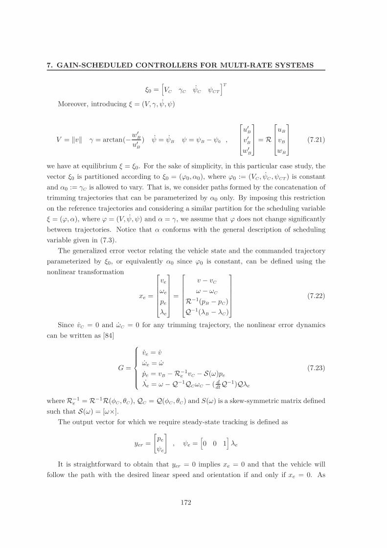
7. GAIN-SCHEDULED CONTROLLERS FOR MULTI-RATE SYSTEMS
*0 =%VC .C 5C 5CT
&T
Moreover, introducing * = (V, ., 5, 5)
V = )v) . = arctan(0w)B
u)B
) 5 = 5B 5 = 5B 0 50 ,
0
112
u)B
v)B
w)B
3
445 = R
0
112
uB
vB
wB
3
445 (7.21)
we have at equilibrium * = *0. For the sake of simplicity, in this particular case study, thevector *0 is partitioned according to *0 = (70, $0), where 70 := (VC , 5C , 5CT ) is constantand $0 := .C is allowed to vary. That is, we consider paths formed by the concatenation oftrimming trajectories that can be parameterized by $0 only. By imposing this restrictionon the reference trajectories and considering a similar partition for the scheduling variable* = (7, $), where 7 = (V, 5, 5) and $ = ., we assume that 7 does not change significantlybetween trajectories. Notice that $ conforms with the general description of schedulingvariable given in (7.3).
The generalized error vector relating the vehicle state and the commanded trajectoryparameterized by *0, or equivalently $0 since 70 is constant, can be defined using thenonlinear transformation
xe =
0
111112
ve
&e
pe
"e
3
444445=
0
111112
v 0 vC
& 0 &C
R!1(pB 0 pC)Q!1("B 0 "C)
3
444445(7.22)
Since vC = 0 and &C = 0 for any trimming trajectory, the nonlinear error dynamicscan be written as [84]
G =
+:::::,
:::::-
ve = v
&e = &
pe = vB 0 R!1e vC 0 S(&)pe
"e = & 0 Q!1QC&C 0 ( ddtQ
!1)Q"e
(7.23)
where R!1e = R!1R(4C , #C), QC = Q(4C , #C) and S(&) is a skew-symmetric matrix defined
such that S(&) = [&#].The output vector for which we require steady-state tracking is defined as
yer =#
pe
5e
$
, 5e =%0 0 1
&"e
It is straightforward to obtain that yer = 0 implies xe = 0 and that the vehicle willfollow the path with the desired linear speed and orientation if and only if xe = 0. As
172

7.4 Trajectory Tracking Control for Autonomous Rotorcraft
mentioned in the next section, the state is assumed available, although at di!erent rates,and thus we have
yem = xe
The linearization of (7.23) about the equilibrium (xe = 0, u = uC), or equivalently, thelinearization of (7.20) about $0, can be written in compact form as
Gl($0) =
+:::,
:::-
xe' = Ae($0)xe' + Be($0)u'
yem' = xe'
yer' = Cer($0)xe'
, (7.24)
where xe' = xe, u' = u 0 uC , yer' = yer, yem' = yem, and Cer($0) =#0 I3 00 0 [0 0 1]
$
. For
details on the matrices of the linearization see [84]. Note that, Gl($0) is the parameterizedlocal system model, for which the controller is to be designed.
7.4.3 Multi-rate Characteristics of the Sensors
As already mentioned, for an autonomous vehicle the dynamic and kinematic state-variablescomprise linear and angular velocities, position and orientation which are usually availableat di!erent rates (for example the position is typically measured by a GPS receiver whichimposes a slow rate). In the present chapter we assume that the state variables of thevehicle corresponding to linear and angular velocities and orientation are measured at asampling rate of 50 Hz, which corresponds to a sampling period ts = 0.02 s, whereas theposition variables are measured at a sampling rate of 2.5 Hz, corresponding to a samplingrate of tsp = 0.4 s. The actuators are assumed synchronous and updated at a rate of50 Hz. According to these sampling rates, the h-periodic matrices (mk, (rk and )k thatcharacterize the multi-rate setup, are given by
)k = I4
(mk =<
I12 k = 0diag([13 13 03 13]) otherwise
(rk =<
I4 k = 0diag([03 1]) otherwise
, k = 0, .., h 0 1.
where h = 20.
7.4.4 Controller Synthesis and Implementation
The commonly used method for the design of a family of controllers for the parameterizedfamily of models, which is also adopted in the present chapter, comprises the following steps:
173

7. GAIN-SCHEDULED CONTROLLERS FOR MULTI-RATE SYSTEMS
i) obtain a finite set of parameter values from the discretization of the continuous parameterspace, ii) synthesize a linear controller for each linear plant, described by (7.24), obtainedfrom the linearization of the nonlinear plant for each value of the schedule parameter, iii)interpolate the coe"cients of the linear controllers to obtain a continuously parameter-varying controller.
We have restricted the parameter space to $ = ., which means that the synthesizedcontrollers are valid in operating conditions where the remaining parameters 7 = (V, 5, 5)do not change significantly about nominal values (VC , 5C , 5C). The finite set of values forthe discretization of this one-dimensional parameter space was chosen to be
$0 = {$0i} = [-50 -40 -30 -20 -10 0 10 20 30 40 50] 3
180 rad.
so that the conditions under which the vehicle is expected to operate include straightlines 5C = 0 and z-aligned helices 5C 1= 0, with a flight path angle between -50 and50 degrees, that the vehicle is required to follow with constant velocity, yaw rate andorientation with respect to the path ((V, 5, 5) = (VC , 5C , 5C)).
For each fixed value of $0, the standard output feedback H2 formulation for periodicsystem was used to synthesize a controller CK for the augmented system Ga where Ad,Bd, Cd are the discretizations of system matrices of (7.24). Notice that Ga has a numberof states equal to n + m + nyr = 12 + 4 + 12 = 28 and a number of outputs equal tonym + nyr = 12 + 4 = 16. For an h-periodic system G of the form
G :=
+::,
::-
xk+1 = Akxk + B1kwk + B2kuk
zk = C1kxk + D11kwk + D12kuk
yk = C2kxk + D21kwk + D22kuk
(7.25)
with D11k = 0, the H2 control problem can be interpreted as the problem of finding alinear h-periodic controller K : yk ,- uk that minimizes the average over one period of thenorms of the impulse responses of the closed-loop system,
Gcl :=<
xk+1 = Ak xk + B1kwk
zk = C1kxk
which can be written as
)Gcl)2 = (1h
h!1*
j=0
nw*
i=1)Gcl((k 0 j)ei)2) 1
2 . (7.26)
where Gcl((k 0 j)ei denotes the output response to an impulse applied at input i and timej. The solution to this problem can be obtained by solving two periodic Riccati equations[8] or by the solution of two LMI optimization problems [93]. The matrices associatedwith the performance channel wk ,- zk are typically used as tuning knobs to improve the
174
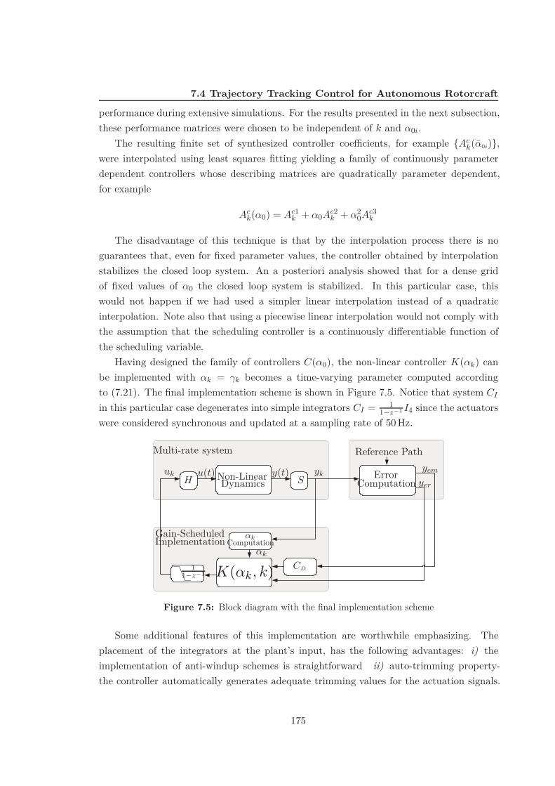
7.4 Trajectory Tracking Control for Autonomous Rotorcraft
performance during extensive simulations. For the results presented in the next subsection,these performance matrices were chosen to be independent of k and $0i.
The resulting finite set of synthesized controller coe"cients, for example {Ack($0i)},
were interpolated using least squares fitting yielding a family of continuously parameterdependent controllers whose describing matrices are quadratically parameter dependent,for example
Ack($0) = Ac1
k + $0Ac2k + $2
0Ac3k
The disadvantage of this technique is that by the interpolation process there is noguarantees that, even for fixed parameter values, the controller obtained by interpolationstabilizes the closed loop system. An a posteriori analysis showed that for a dense gridof fixed values of $0 the closed loop system is stabilized. In this particular case, thiswould not happen if we had used a simpler linear interpolation instead of a quadraticinterpolation. Note also that using a piecewise linear interpolation would not comply withthe assumption that the scheduling controller is a continuously di!erentiable function ofthe scheduling variable.
Having designed the family of controllers C($0), the non-linear controller K($k) canbe implemented with $k = .k becomes a time-varying parameter computed accordingto (7.21). The final implementation scheme is shown in Figure 7.5. Notice that system CI
in this particular case degenerates into simple integrators CI = 11!z!1 I4 since the actuators
were considered synchronous and updated at a sampling rate of 50 Hz.
Non-LinearDynamics
CD11!z!1
Reference Path
ErrorComputation
u(t) y(t)uk yk
K($k, k)
$kComputation
SHyem
yer
$k
Multi-rate system
Gain-ScheduledImplementation
Figure 7.5: Block diagram with the final implementation scheme
Some additional features of this implementation are worthwhile emphasizing. Theplacement of the integrators at the plant’s input, has the following advantages: i) theimplementation of anti-windup schemes is straightforward ii) auto-trimming property-the controller automatically generates adequate trimming values for the actuation signals.
175

7. GAIN-SCHEDULED CONTROLLERS FOR MULTI-RATE SYSTEMS
Though in the present case simple integrators are being used, the same advantages wouldhold if the inputs were updated at di!erent rates and the integrators took the form of )I .
7.4.5 Simulation Results
We start with a simple example that compares the performance of a multi-rate guid-ance and control law with that obtained using a standard single-rate H2 compensatordesigned using equivalent weighting matrices. First, we compare the values of the closed-loop H2 norms while changing the rate of the linear position measurement and keepingthe sampling periods of the other outputs and of the input at ts = 0.02 s. The peri-odic H2 controllers were synthesized for a single operating condition, characterized by*0 =
%VC .C 5C 5CT
&T
=%1 m.s!1 0 rad 0 rad.s!1 0 rad
&T
. The results are shown inTable 7.1.
Notice that when the sampling rate of the linear position measurement equals thesampling rate of the other outputs (ts = 0.02 s), the multi-rate set-up particularizes to thesingle-rate case and the periodic H2 controller is equivalent to a standard discrete-time H2controller. As expected the performance of the closed-loop system, given in terms of theH2 norm, deteriorates as the sampling period for the linear position increases. In order toassess the impact of this performance loss on the tracking response of the vehicle, a simplemaneuver task is set up for the rotorcraft. During the maneuver the vehicle is required tofollow a path with constant velocity VC = 1 m.s!1 and constant orientation with respectto the path, consisting of: i) a level flight segment along the x axis, ii) a climbing rampwith a flight path angle of .C = .
6 rad, iii) a level flight segment along the x axis. Again-scheduled controller was synthesized following the procedure given in Section 7.4 forconstant parameters 70 = (VC , 5C , 5CT ) = (1 m.s!1, 0 rad.s!1, 0 rad). For the single-ratecase, all the outputs are measured at a sampling rate of ts = 0.02 s, and for the multi-ratecase, the sampling rates are given according to Section 7.4.7.4.3. The results comparingthese two cases, which include the temporal evolution of the actuation, dynamic variables v
and &, and kinematic errors pE = pB 0pC = [xE yE zE]T and "E = "B 0"C = [4E #E 5E]T ,are shown in Figures 7.6 and 7.7.
As expected, we can notice some degradation in the actuation and error responsesfor the multi-rate case in comparison with the single-rate case. Nevertheless, while theproposed method takes into account the multi-rate characteristics of the sensors, it alsoachieves good tracking performance and displays a smooth behavior throughout the di!er-
Table 7.1: H2 closed-loop values for di!erent position sampling rates
Linear position sampling period tsp(s) 0.02 0.04 0.1 0.2 0.4Closed loop H2 norm )Gcl)2 10.40 11.08 12.18 13.15 14.27
176
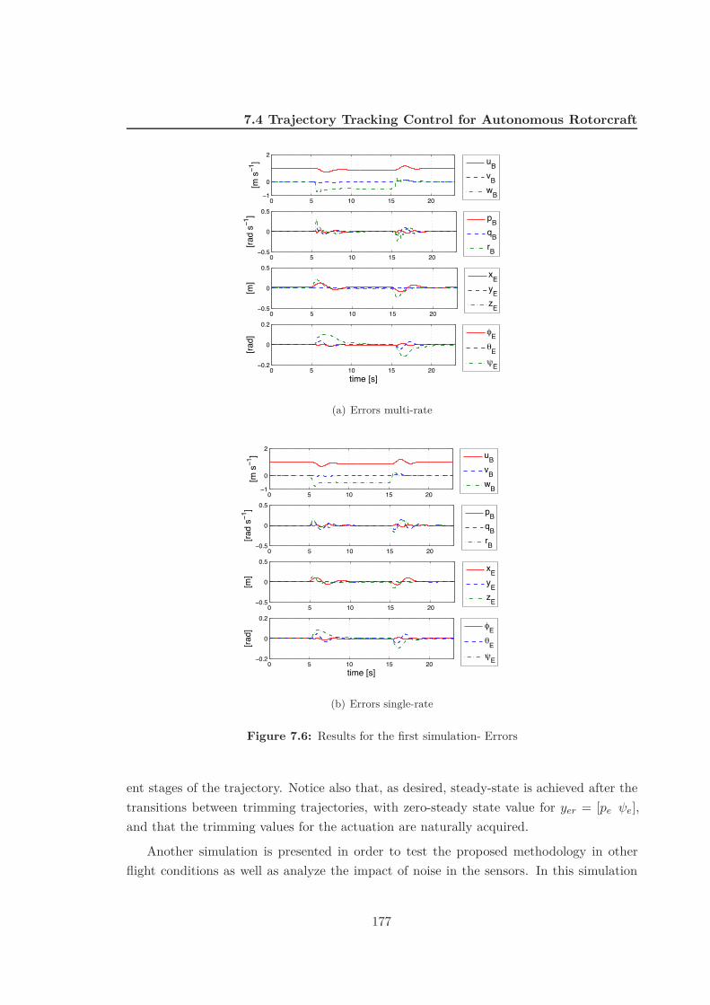
7.4 Trajectory Tracking Control for Autonomous Rotorcraft
0 5 10 15 20−1
0
2
[m s−1
]
uBvBwB
0 5 10 15 20−0.5
0
0.5
[rad
s−1 ]
pBqBrB
0 5 10 15 20−0.5
0
0.5
[m]
xEyEzE
0 5 10 15 20−0.2
0
0.2
time [s]
[rad]
qEeEsE
(a) Errors multi-rate
0 5 10 15 20−1
0
2
[m s−1
]
uBvBwB
0 5 10 15 20−0.5
0
0.5
[rad
s−1 ]
pBqBrB
0 5 10 15 20−0.5
0
0.5
[m]
xEyEzE
0 5 10 15 20−0.2
0
0.2
time [s]
[rad]
qEeEsE
(b) Errors single-rate
Figure 7.6: Results for the first simulation- Errors
ent stages of the trajectory. Notice also that, as desired, steady-state is achieved after thetransitions between trimming trajectories, with zero-steady state value for yer = [pe 5e],and that the trimming values for the actuation are naturally acquired.
Another simulation is presented in order to test the proposed methodology in otherflight conditions as well as analyze the impact of noise in the sensors. In this simulation
177

7. GAIN-SCHEDULED CONTROLLERS FOR MULTI-RATE SYSTEMS
0 5 10 15 200
0.05
0.1
e 0[rad]
0 5 10 15 20−0.05
0
0.05e s[ra
d]
0 5 10 15 20−0.05
0
0.05
e c[rad]
0 5 10 15 200.05
0.1
0.15
e tr[rad]
time [s]
(a) Actuation multi-rate
0 5 10 15 200
0.05
0.1
e 0[rad]
0 5 10 15 20−0.05
0
0.05
e s[rad]
0 5 10 15 20−0.05
0
0.05
e c[rad]
0 5 10 15 200.05
0.1
0.15
e tr[rad]
time [s]
(b) Actuation single-rate
Figure 7.7: Results for the first simulation- Actuation
the vehicle is required to follow a path with constant velocity VC = 5m.s!1 and constantorientation with respect to the path, consisting of i) a level flight segment along the x axis,ii) a climbing helix with a flight path angle of .C = 0.29 rad and yaw rate 5C = 0.26 rad.s!1,iii) a level flight segment along the x axis. The controller is synthesized according tothe methodology presented in Section 7.4 for constant parameters 70 = (VC , 5C , 5CT ) =(5 m.s!1, 0 rad.s!1, 0 rad) and the weights of the H2 controller synthesis problem, describedin (7.25) are changed to accommodate for the di!erent operating conditions. We have
178
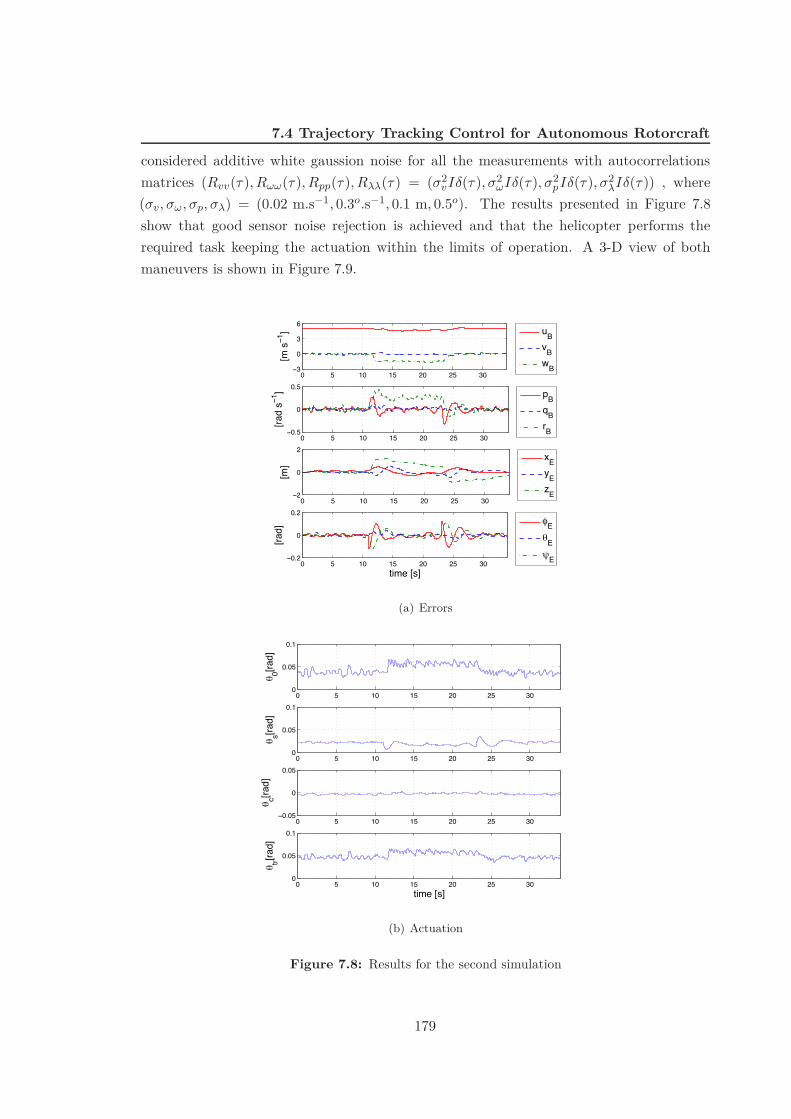
7.4 Trajectory Tracking Control for Autonomous Rotorcraft
considered additive white gaussion noise for all the measurements with autocorrelationsmatrices (Rvv(!), R44(!), Rpp(!), R$$(!) = (,2
vI((!), ,24I((!), ,2
pI((!), ,2$I((!)) , where
(,v, ,4, ,p, ,$) = (0.02 m.s!1, 0.3o.s!1, 0.1 m, 0.5o). The results presented in Figure 7.8show that good sensor noise rejection is achieved and that the helicopter performs therequired task keeping the actuation within the limits of operation. A 3-D view of bothmaneuvers is shown in Figure 7.9.
0 5 10 15 20 25 30−3
0
3
6
[m s−1
]
uBvBwB
0 5 10 15 20 25 30−0.5
0
0.5
[rad
s−1 ]
pBqBrB
0 5 10 15 20 25 30−2
0
2
[m]
xEyEzE
0 5 10 15 20 25 30−0.2
0
0.2
time [s]
[rad]
qEeEsE
(a) Errors
0 5 10 15 20 25 300
0.05
0.1
e 0[rad]
0 5 10 15 20 25 300
0.05
0.1
e s[rad]
0 5 10 15 20 25 30−0.05
0
0.05
e c[rad]
0 5 10 15 20 25 300
0.05
0.1
e tr[rad]
time [s]
(b) Actuation
Figure 7.8: Results for the second simulation
179

7. GAIN-SCHEDULED CONTROLLERS FOR MULTI-RATE SYSTEMS
05101520
-6
-4
-2
0
2
x[m]
z[m
]
(a) First Simulation
0
10
20
30
40
50
60
70
-5 0 5 10 15 20 25 30 35 40
-15
-10
-5
0
5
y[m]
x[m]
z[m
]
(b) Second Simulation
Figure 7.9: Rotorcraft Maneuvers
7.5 Further Comments and References
Over the last few decades there has been a surge of interest in the development of ef-ficient and reliable guidance and control algorithms for unmanned vehicles. An endlessnumber of applications are reported in the literature, ranging from underwater geologicalsurveillance [75] to spacecraft missions [93].
Traditionally, the guidance and control problem for autonomous vehicles involves thedesign of an inner and an outer loop [86]. The inner loop is designed to stabilize thevehicle dynamics and usually requires a high sampling rate, whereas the outer loop designrelies essentially on the vehicle’s kinematic model, converting tracking errors into innerloop commands, and is amenable to a lower sampling rate. As explained in [84], sincethe two systems, kinematics and dynamics, are e!ectively coupled, stability and adequateperformance of the combined systems are not guaranteed. An interesting feature of thistechnique is that, since the kinematic variables are commonly available at lower rates(consider for example the case of a GPS receiver), the design of the di!erent loops atdi!erent rates often handles naturally the multi-rate characteristic of the sensors.
180

7.5 Further Comments and References
Another line of work, presented in [22], [50], [84] proposes and integrated solution for theguidance and control problem. This solution amounts to applying a conveniently definedpath-dependent transformation to the vehicle’s equations of motion, which involves bothkinematic and dynamic variables of the vehicle. In this new space, referred to as error-space,the problems of trajectory tracking or path-following reduce to the problem of driving thisnewly-defined error to zero. The family of error transformations presented in [22], [50], [84]have the notable property of guaranteeing that the linearization of the error dynamics istime-invariant along trimming trajectories, which comprise arbitrary straight lines and z-aligned helices. Since the vehicle’s dynamic behavior changes considerably throughout itsflight envelope, gain-scheduling control laws, which have become a standard solution inflight control systems, are typically used. In this setting, the multi-rate characteristics ofthe sensors have been traditionally handled by the navigation system design [75] withoutguaranteeing the performance (or even the stability) of the overall closed loop system,although the problem can be formulated as a control design problem.
This chapter follows the line of work reported in [22], [50], [84], adopting the integratedguidance and control approach and proposes a novel method to take into account themulti-rate characteristics of the sensors in the controller design. To this e!ect, theoreticalresults are first derived which make use of the existing background for multi-rate systemsand gain-scheduling theory. The theory for multi-rate systems is intimately related withthe theory of periodically time-varying systems. See, for example, [78] and the referencestherein for early work on the subject and [61] for more recent developments. Noteworthyis the bulk of work in this field by Bittanti, Colaneri and co-workers. With particularinterest to the present chapter are the definitions of stabilizability and detectability forperiodic systems [7], and the solutions of the problems of regulation for square multi-ratesystems [19], output stabilization for periodic systems [16], and LQG optimal control formulti-rate systems [17]. In the field of gain-scheduling an excellent survey can be foundin [81].
The velocity implementation, was presented in [51], [52] and is also discussed in [53,Ch. 12], [81] which is related with the work presented herein, provides a simple solutionfor the implementation of controllers with integral action that satisfies the linearizationproperty.
181

7. GAIN-SCHEDULED CONTROLLERS FOR MULTI-RATE SYSTEMS
182
8
Conclusions and Future Work
In this thesis, we addressed several scenarios in Networked Control Systems. We modeledthese scenarios under the framework of impulsive systems and stochastic hybrid systemsand we derived several theoretical results for such systems, which directly entails propertiesfor the networked control system. The results were shown to be of interest in other researchareas. In a nutshell, the main conclusions are as follows:
• The framework of Volterra renewal type equations is a useful framework for the anal-ysis of linear networked control systems with independent and identically distributedtime between transmissions, and with several other features amenable with a finite-state machine model. This approach leads to interesting results, such as providing astability condition in terms of the Nyquist criterion for the analysis of these networkedcontrol systems.
• Networked Control Systems with asynchronous renewal transmissions can be modeledby piecewise deterministic processes. Using tools that borrow from this latter classof systems, one can provide a necessary and su"cient stability test in terms of thecomputation of the spectral radius of an integral operator.
• One can construct a class of dynamic protocols that outperform static protocols byconstruction. In an optimal control framework where the intent is to simultaneouslydesign the control law and the protocols, our approach, based on a rollout strategy,leads to a distributed algorithm which nodes can run independently.
• There is a solution to the output regulation problem for multi-rate systems, evenin the case where the number of outputs is larger than the number of inputs. Inthe special case of constant references, this same solution is useful to tackle thegain-scheduling problem for non-linear systems.
There are several directions for future work. We include here the following:
183

8. CONCLUSIONS AND FUTURE WORK
• Direct design. The problem of directly designing a controller in the setting of Chap-ters 2, Chapter 3, and Chapter 4 should be looked into with more detail. We haveshown in [AHS09a] how to optimally design a state feedback controller for simple net-worked control set-ups as in the framework of Chapter 2. An interesting direction forfuture work is to extend these results for output feedback. In particular one could askif the separation or equivalence principle holds, i.e., if the optimal output feedbackcontroller could be obtained by separately computing the optimal controller and theoptimal state observer. In the case of networked control systems with asynchronousrenewal networks, as in Chapter 4, the problem was not addressed, and thereforeremains open.
• Dynamic Protocols. The rollout strategy that we propose to solve the simultaneouscontroller and protocol design may be in general computationally demanding to beimplemented on-line. Therefore, a direction for future work is to propose heuristicsthat approximate this policy, while being within reasonable computational burdensfor on-line implementation.
• Gain-Scheduling structure. The gain-scheduling structure that we propose for multi-rate systems is inspired on the velocity implementation. However, this implementa-tion involves a di!erentiation, which may introduce significant noise at the input ofthe gain-scheduled controller, and in general this can have malicious e!ects for theclosed-loop. An interesting direction for future work would be to obtain a structurethat also satisfies the linearization property, but does not require di!erentiation.
• Output regulator Controller Structure. It would also be interesting to obtain a con-troller structure that does not need to di!erentiate the inputs in the output regulationproblem, since di!erentiation may lead to large transitory behavior.
• Nonlinear Networked Control Systems. The Theorem 24 provides an analog resultto a well-known stability results for non-linear stochastic hybrid systems. One canexplore this fact by posing several problems for non-linear closed-loops with inde-pendent and indentically distributed intervals between transmissions, which parallelproblems for non-linear deterministic systems.
• Assumptions on the intervals between transmissions. We argued that in the Ether-net and Wireless 802.11 networks the times between transmissions are independentand identically distributed, following similar reasonings to other works in the litera-ture [44]. A direction for future work is to confirm this assumption experimentally.
184

Bibliography
[1] Karl Astrom. Introduction to stochastic control theory. Academic Press, 1970.
[2] Conway J. B. A Course in Functional Analysis. Springer-Verlag, New York, 1985.
[3] Richard Bellman. The stability of solutions of linear di!erential equations. Duke Math.J., (10):643–647, 1991.
[4] A. Bergen. Stability of systems with randomly time-varying parameters. AutomaticControl, IRE Transactions on, 5(4):265–269, Sep 1960.
[5] Dimitri P. Bertsekas. Dynamic Programming and Optimal Control. Athena Scientific,2005.
[6] B. H. Bharucha. On the stability of randomly varying systems. PhD thesis, Universityof California, Berkeley, CA„ July 1961.
[7] S. Bittanti and P. Bolzern. Stabilizability and detectability of linear periodic systems.System & Control Letters, 6(2):141–146, 1985.
[8] S. Bittanti, P. Colaneri, and G. Nicolao. The di!erence periodic riccati equation for theperiodic prediction problem. IEEE Transactions on Automatic Control, 33(8):706–712,August 1988.
[9] Sergio Bittanti and Patrizio Colaneri. Invariant representations of discrete-time periodicsystems. Automatica, 36(12):1777 – 1793, 2000.
[10] S. Boyd, A. Ghosh, B. Prabhakar, and D. Shah. Randomized gossip algorithms.Information Theory, IEEE Transactions on, 52(6):2508 – 2530, 2006.
[11] Stephen Boyd and Lieven Vandenberghe. Convex Optimization. Cambridge UniversityPress, 2004.
[12] F. Bullo, J. Cortes, and S. Martınez. Distributed Control of Robotic Networks. Ap-plied Mathematics Series. Princeton University Press, 2009. Electronically available athttp://coordinationbook.info.
185

BIBLIOGRAPHY
[13] C. I. Byrnes and A. Isidori. Output regulation for nonlinear systems: an overview.International Journal of Robust and Nonlinear Control, 10:323–337, 2000.
[14] F. Chatelin. Spectral approximation of linear operators. Academic Press, 1983.
[15] Tongwen Chen and Bruce Francis. Optimal Sampled-Data Control Systems. Springer-Verlag, 1995.
[16] P. Colaneri. Output stabilization via pole placement of discrete-time linear periodicsystems. IEEE Transactions on Automatic Control, 36(6):739–742, June 1991.
[17] P. Colaneri and G. Nicolao. Multirate lqg control of continuous-time stochastic sys-tems. Automatica, 31(4):591–596, April 1995.
[18] P. Colaneri, R. Scattolini, and N. Schiavoni. Stabilization of multirate sampled-datalinear systems. Automatica, 26(2):377 – 380, 1990.
[19] P. Colaneri, R. Scattolini, and N. Schiavoni. Regulation of multirate sampled-datasystems. Control-Theory and Advanced Technology, 7(3):429–441, 1991.
[20] P. Colaneri, R. Scattolini, and N. Schiavoni. Lqg optimal control of multirate sampled-data systems. IEEE Transactions on Automatic Control, 37(5):675–682, May 1992.
[21] O. L. V. Costa, M.D. Fragoso, and R.P.Marques. Discrete-Time Markov Jump LinearSystems. Springer, 2005.
[22] R. Cunha, D. Antunes, and C. Gomes, P. Silvestre. A path-following preview controllerfor autonomous air vehicles. In AIAA Guidance, Navigation, and Control Conference,Keystone, August 2006. AIAA.
[23] R. Cunha and C. Silvestre. Dynamic modeling and stability analysis of model-scalehelicopters with bell-hiller stabilizing bar. In AIAA Guidance, Navigation, and ControlConference, Austin, TX, August 2003. AIAA.
[24] Dragan Dacic and Dragan Nesic. Observer design for wired linear networked controlsystems using matrix inequalities. Automatica, 44(11):2840 – 2848, 2008.
[25] M. H. A. Davis. Markov Models and Optimization. Chapman & Hall, London, UK,1993.
[26] E. Davison. The output control of linear time-invariant multivariable systems withunmeasurable arbitrary disturbances. Automatic Control, IEEE Transactions on,17(5):621 – 630, oct. 1972.
186
BIBLIOGRAPHY
[27] M. C. F. Donkers, W. P. M. H. Heemels, D. Bernadini, A. Bemporad, and V. Shneer.Stability analysis of stochastic networked control systems. Accepted for Automatica,2011.
[28] M.C.F. Donkers, W.P.M.H. Heemels, N. van de Wouw, and L. Hetel. Stability analysisof networked control systems using a switched linear systems approach. AutomaticControl, IEEE Transactions on, 56(9):2101 –2115, sept. 2011.
[29] Florian Dorfler and Francesco Bullo. Synchronization and transient stability in powernetworks and non-uniform kuramoto oscillators. In Proceedings of the American ControlConference 2010, Baltimore, Maryland, USA, July 2010.
[30] W. Dunbar and D. Caveney. Distributed receding horizon control of vehicle platoons:Stability and string stability. Automatic Control, IEEE Transactions on, PP(99):1,2011.
[31] N. Elia and S.K. Mitter. Stabilization of linear systems with limited information.Automatic Control, IEEE Transactions on, 46(9):1384 –1400, September 2001.
[32] X. Feng, K.A. Loparo, Y. Ji, and H.J. Chizeck. Stochastic stability properties of jumplinear systems. Automatic Control, IEEE Transactions on, 37(1):38–53, Jan 1992.
[33] B. Francis and W. M. Wonham. The internal model principle of control theory. Au-tomatica, 12:457–465, September 1976.
[34] Bruce A. Francis. The linear multivariable regulator problem. SIAM J. ControlOptim., 15(3):486–505, May 1977.
[35] H. Fujimoto and Y. Hori. Visual servoing based on intersample disturbance rejectionby multirate sampling control-time delay compensation and experimental verification.In 40th IEEE Conference on Decision and Control, Orlando, FL, USA, December 2001.
[36] J.C. Geromel and P. Colaneri. Stability and stabilization of discrete time switchedsystems. International Journal of Control, 79(7):719–728, 2006.
[37] B. Ghosh, B. Basu, and M. Mahony. Multivariate short-term tra"c flow forecastingusing time-series analysis. IEEE Transactions on Intelligent Transportation Systems,10(2), 2009.
[38] Mrinal K. Ghosh, Aristotle Arapostathis, and Steven I. Marcus. Ergodic controlof switching di!usions. SIAM Journal of Control and Optimization, 35:1952–1988,November 1997.
187

BIBLIOGRAPHY
[39] G. Gripenberg, S. O. Londen, and O. Sta!ans. Volterra Integral and Functional Equa-tions. Cambridge University Press, 1990.
[40] Kuoruey Han. Randomly sampled-data control systems, 1990. phd thesis, UCLA.
[41] Floyd B. Hanson. Applied Stochastic Processes and Control for Jump Di"usions:Modeling, Analysis, and Computation. SIAM, New York, NY, USA, 2007.
[42] Joao Hespanha, Antonio Ortega, and Lavanya Vasudevan. Towards the control oflinear systems with minimum bit-rate. In In Proc. of the Int. Symp. on the MathematicalTheory of Networks and Syst, 2002.
[43] Joao P. Hespanha, Payam Naghshtabrizi, and Yonggang Xu. A survey of re-cent results in networked control systems. Proc. of IEEE Special Issue on Tech-nology of Networked Control Systems, 95(1):138–162, January 2007. Available athttp://www.ece.ucsb.edu/˜hespanha/published.
[44] Joao P. Hespanha and Andrew R. Teel. Stochastic impulsive systems driven by renewalprocesses. In 17th International Symposium on Mathematical Theory of Networks andSystems (MTNS06), Kyoto, Japan, July 2006.
[45] Joao Pedro Hespanha. A model for stochastic hybrid systems with application to com-munication networks. Nonlinear Analysis, Special Issue on Hybrid Systems, 62(8):1353–1383, September 2005.
[46] Roger A Horn and Charles R. Johnson. Topics in matrix analysis. Cambridge Uni-versity Press, New York, NY, USA, 1994.
[47] Jianghai Hu, John Lygeros, and Shankar Sastry. Towards a theory of stochastic hybridsystems. In In Third International Workshop on Hybrid Systems: Computation andControl, pages 160–173. Springer, 2000.
[48] Janssen, Jacques, Manca, and Raimondo. Applied Semi-Markov Processes. Springer-Verlag, 2006.
[49] B. Johansson, T. Keviczky, M. Johansson, and K.H. Johansson. Subgradient methodsand consensus algorithms for solving convex optimization problems. In Decision andControl, 2008. CDC 2008. 47th IEEE Conference on, pages 4185 –4190, 2008.
[50] I. Kaminer, A. Pascoal, E. Hallberg, and C. Silvestre. Trajectory tracking for au-tonomous vehicles: An integrated approach to guidance and control. AIAA Journal ofGuidance, Control, and Dynamics, 21(1):29–38, 1998.
188

BIBLIOGRAPHY
[51] I. Kaminer, A. Pascoal, P. Khargonekar, and E. Coleman. A velocity algorithm forthe implementation of gain-scheduled controllers. Technical report, Naval PostgraduateSchool, 1994.
[52] I. Kaminer, A. Pascoal, P. Khargonekar, and E. Coleman. A velocity algorithm forthe implementation of gain-scheduled controllers. Automatica, 31(8):1185–1191, August1995.
[53] Hassan Khalil. Nonlinear Systems, Third Edition. Prentice Hall, Upper Saddle River,NJ, 2002.
[54] Oliver Knill. On haussdor!’s moment problem in higher dimensions. Technical report,University of Arizona, 2000.
[55] W. L. De Koning. Infinite horizon optimal control of linear discrete time systems withstochastic parameters. Automatica, 18(4), 1982.
[56] M. A. Krasnoselskii, Je. A. Lifshits, and A. V. Sobolev. Positive linear systems : themethod of positive operators. Heldermann, Verlag, Berlin, 1989.
[57] C. Kubrusly and O. Costa. Mean square stability conditions for discrete stochasticbilinear systems. Automatic Control, IEEE Transactions on, 30(11):1082–1087, Nov1985.
[58] James F. Kurose and Keith W. Ross. Computer Networking: A Top-Down Approach(3th Edition). Addison Wesley, 2005.
[59] H. Kushner and L. Tobias. On the stability of randomly sampled systems. AutomaticControl, IEEE Transactions on, 14(4):319–324, Aug 1969.
[60] Harold J. Kushner. Stochastic Stability and Control. Academic Press, New York, NY,USA, 1967.
[61] S. Lall and G. Dullerud. An lmi solution to the robust synthesis problem for multi-ratesampled-data systems. Automatica, 37, 2001.
[62] D. A. Lawrence. Stability analysis of nonlinear sampled-data systems. In 36th IEEEConference on Decision and Control, San Diego, CA, USA, December 1997.
[63] D.A. Lawrence and E.A. Medina. Output regulation for linear systems with sampledmeasurements. volume 3, pages 2044 –2049 vol.3, 2001.
[64] Peter Linz. Analytical and Numerical Methods for Volterra Equations. SIAM Studiesin Applied Mathematics 7, 1985.
189
BIBLIOGRAPHY
[65] S. Longhi. Structural properties of multirate sampled-data systems. Automatic Con-trol, IEEE Transactions on, 39(3):692 –696, mar. 1994.
[66] Michel Mariton. Jump Linear Systems in Automatic Control. Marcel Dekker Inc, NewYork, NY, USA, 1990.
[67] Cai Meng, Tianmiao Wang, Wusheng Chou, Sheng Luan, Yuru Zhang, and ZengminTian. Remote surgery case: robot-assisted teleneurosurgery. In Robotics and Automa-tion, 2004. Proceedings. ICRA ’04. 2004 IEEE International Conference on, 2004.
[68] R.A. Meyer and C.S. Burrus. A unified analysis of multirate and periodically time-varying digital filters. IEEE Trans. Circuits Systems, 22:162–168, 1975.
[69] L.A. Montestruque and P. Antsaklis. Stability of model-based networked control sys-tems with time-varying transmission times. Automatic Control, IEEE Transactions on,49(9):1562–1572, Sept. 2004.
[70] Irinel Constantin Morarescu and Carlos Canudas De Wit. Highway tra"c model-based density estimation. In Proceedings of the American Control Conference 2011,San Francisco, USA, July 2011.
[71] J.R. Moyne and D.M. Tilbury. The emergence of industrial control networks formanufacturing control, diagnostics, and safety data. Proceedings of the IEEE, 95(1):29–47, 2007.
[72] Girish N. Nair and Robin J. Evans. Exponential stabilisability of finite-dimensionallinear systems with limited data rates. Automatica, 39(4):585 – 593, 2003.
[73] D. Nesic and A.R. Teel. Input-output stability properties of networked control systems.Automatic Control, IEEE Transactions on, 49(10):1650–1667, Oct. 2004.
[74] Y. Nesterov and A. Nemirovskii. Interior-Point Polynomial Methods in Convex Pro-gramming. Society for Industrial and Applied Mathematics, 1994.
[75] P. Oliveira and A. Pascoal. On the design of multirate complementary filters for au-tonomous marine vehicle navigation. In GCUV2003 - 1st IFAC Workshop on Guidanceand Control of Underwater Vehicles, Newport, UK, 2003.
[76] G. Pola, M.L. Bujorianu, J. Lygeros, and M.D. Di Benedetto. Stochastic hybridmodels: An overview. In IFAC Conference on Analysis and Design of Hybrid Systems,pages 16–18, St. Malo, June 2003. Springer.
[77] R. Sanfelice R. Goebel and A.R. Teel. Hybrid dynamical systems. robust stability andcontrol for systems that combine continuous-time and discrete-time dynamics. IEEEControl Systems Magazine, 29(2):28–93, 2009.
190
BIBLIOGRAPHY
[78] H. Rahmani and G. Franklin. A new optimal multirate control of linear periodic andtime-invariant systems. IEEE Transactions on Automatic Control, 35(4):406–415, April1990.
[79] Sidney I. Resnick. Adventures in stochastic processes. Birkhauser Verlag, Basel,Switzerland, Switzerland, 1992.
[80] Walter Rudin. Real and complex analysis, 3rd ed. McGraw-Hill, Inc., New York, NY,USA, 1987.
[81] W. Rugh and J. Shamma. Research on gain scheduling. Automatica, 36:1401–1425,October 2000.
[82] R. Scattolini and N. Schiavoni. On the output control of multirate systems subjectto arbitrary exogenous signals. Automatic Control, IEEE Transactions on, 38(4):643–646, apr. 1993.
[83] L. Schenato, B. Sinopoli, M. Franceschetti, K. Poolla, and S.S. Sastry. Foundations ofcontrol and estimation over lossy networks. Proceedings of the IEEE, 95(1):163 –187,2007.
[84] C. Silvestre, A. Pascoal, and I. Kaminer. On the design of gain-scheduled trajectorytracking controllers. International Journal of Robust and Nonlinear Control, 12:797–839, 2002.
[85] Michael Spivak. Calculus on manifolds. A modern approach to classical theorems ofadvanced calculus. W. A. Benjamin, Inc., New York-Amsterdam, 1965.
[86] B. Stevens and F. Lewis. Aircraft Control and Simulation. John Wiley & Sons, NewYork, USA, 1992.
[87] M. Tabbara and D. Nesic. Input output stability of networked control systemswith stochastic protocols and channels. Automatic Control, IEEE Transactions on,53(5):1160–1175, June 2008.
[88] M. Tabbara, D. Nesic, and A.R. Teel. Stability of wireless and wireline networkedcontrol systems. Automatic Control, IEEE Transactions on, 52(9):1615 –1630, sep.2007.
[89] Mohammad Tabbara and Dragan Nesic. Stability of networked control systems withstochastic protocols. In American Control Conference, 2007, New York City, USA, July2007.
191
BIBLIOGRAPHY
[90] G.C. Walsh and Hong Ye. Scheduling of networked control systems. Control SystemsMagazine, IEEE, 21(1):57 –65, feb. 2001.
[91] G.C. Walsh, Hong Ye, and L.G. Bushnell. Stability analysis of networked controlsystems. Control Systems Technology, IEEE Transactions on, 10(3):438 –446, may.2002.
[92] B. Warneke, M. Last, B. Liebowitz, and K.S.J. Pister. Smart dust: communicatingwith a cubic-millimeter computer. Computer, 34(1):44 –51, January 2001.
[93] J. Stoustrup Wisniewski R. Periodic h2 synthesis for spacecraft attitude control withmagnetometers. AIAA Journal of Guidance, Control, and Dynamics, 27(5):874–881,2004.
[94] Wing Shing Wong and R.W. Brockett. Systems with finite communication bandwidthconstraints. ii. stabilization with limited information feedback. Automatic Control,IEEE Transactions on, 44(5):1049 –1053, May 1999.
[95] W. M. Wonham and J. B. Pearson. Regulation and internal stabilization in linearmultivariable systems. SIAM Journal on Control, 12(1):5–18, 1974.
[96] Z. Wu, M.R. Rajamani, J.B. Rawlings, and J. Stoustrup. Model predictive controlof thermal comfort and indoor air quality in livestock stable. In Proceedings of theEuropean Control Conference, Kos, Greece, July 2007. European Union Control Asso-ciation.
[97] Wei Zhang, M.S. Branicky, and S.M. Phillips. Stability of networked control systems.Control Systems Magazine, IEEE, 21(1):84 –99, feb. 2001.
[98] Kemin Zhou, John C. Doyle, and Keith Glover. Robust and Optimal Control. PrenticeHall, Inc., Upper Saddle River, NJ, 1995.
192
Journal Publications
[AHS11a] Duarte Antunes, Joao Pedro Hespanha, and Carlos Silvestre. Stability of net-worked control systems with asynchronous renewal links: An impulsive systemsapproach. Provisionally accepted for publication in Automatica, Sept. 2011.
[AHS11b] Duarte Antunes, Joao Pedro Hespanha, and Carlos Silvestre. Stochastic hy-brid systems with renewal transitions: Moment analysis with application tonetworked control systems with delays. Submitted to the SIAM Journal onControl and Optimization, Dec. 2011.
[AHS11c] Duarte Antunes, Joao Pedro Hespanha, and Carlos Silvestre. Stochastic net-worked control systems with dynamic protocols. Submitted to the Asian Journalof Control, Dec. 2011.
[AHS11d] Duarte Antunes, Joao Pedro Hespanha, and Carlos Silvestre. Volterra integralapproach to impulsive renewal systems: Application to networked control. Au-tomatic Control, IEEE Transactions on, PP(99):1, 2011. to appear Nov 2012,available online.
[ASC10] Duarte Antunes, Carlos Silvestre, and Rita Cunha. On the design of multi-ratetracking controllers: Application to rotorcraft guidance and control. Interna-tional Journal of Robust and Nonlinear Control, 20:1879–1902, November 2010.
[ASH11] Duarte Antunes, Carlos Silvestre, and Joao Pedro Hespanha. Output regulationfor non-square multi-rate systems. Provisionally accepted for publication in theInternational Journal of Robust and Nonlinear Control, feb. 2011.
193

JOURNAL PUBLICATIONS
194

Conference Publications
[AHHS11a] Duarte Antunes, Maurice Heemels, Joao Pedro Hespanha, and Carlos Silvestre.Scheduling measurements and controls over networks - part i: Rollout strate-gies for protocol design. Submitted to the 2011 Amer. Contr. Conf., Sep.2011.
[AHHS11b] Duarte Antunes, Maurice Heemels, Joao Pedro Hespanha, and Carlos Silvestre.Scheduling measurements and controls over networks - part ii: Rollout strate-gies for simultaneous protocol and controller design. Submitted to the 2011Amer. Contr. Conf., Sep. 2011.
[AHS09a] Duarte Antunes, Joao P. Hespanha, and Carlos Silvestre. Control of impul-sive renewal systems: Application to direct design in networked control. InDecision and Control, 2009 held jointly with the 2009 28th Chinese ControlConference. CDC/CCC 2009. Proceedings of the 48th IEEE Conference on,pages 6882 –6887, dec. 2009.
[AHS09b] Duarte Antunes, Joao P. Hespanha, and Carlos Silvestre. Stability of impulsivesystems driven by renewal processes. In American Control Conference, 2009.ACC ’09., pages 4032 –4037, june 2009.
[AHS10a] Duarte Antunes, Joao P. Hespanha, and Carlos Silvestre. Impulsive systemstriggered by superposed renewal processes. In Decision and Control (CDC),2010 49th IEEE Conference on, pages 1779 –1784, dec. 2010.
[AHS10b] Duarte Antunes, Joao P. Hespanha, and Carlos Silvestre. Stochastic hybridsystems with renewal transitions. In American Control Conference (ACC),2010, pages 3124 –3129, 30 2010-july 2 2010.
[AHS11] Duarte Antunes, Joao P. Hespanha, and Carlos Silvestre. Stochastic networkedcontrol systems with dynamic protocols. In American Control Conference(ACC), 2011, pages 1686 –1691, 29 2011-july 1 2011.
195
CONFERENCE PUBLICATIONS
[ASC07] Duarte Antunes, Carlos Silvestre, and Rita Cunha. On the design of multi-rate tracking controllers: An application to rotorcraft guidance and control.In AIAA Guidance, Navigation, and Control Conference, Hilton Head, SouthCarolina, August 2007. AIAA.
[ASC08a] Duarte Antunes, Carlos Silvestre, and Rita Cunha. Linear parameter varyingcontrol for sampled-data multi-rate systems. In 17th IFAC World Congress,Seoul, Korea, July 2008. IFAC.
[ASC08b] Duarte Antunes, Carlos Silvestre, and Rita Cunha. Multi-rate path-followingcontrol for unmanned air vehicles. In 17th IFAC World Congress, Seoul, Korea,July 2008. IFAC.
196