stochastic circuit design and performance evaluation of...

> REPLACE THIS LINE WITH YOUR PAPER IDENTIFICATION NUMBER (DOUBLE-CLICK HERE TO EDIT) <

1

Abstract—Vector Quantization (VQ) is a general data

compression technique that has a scalable implementation

complexity and potentially a high compression ratio. In this paper,

a novel implementation of VQ using stochastic circuits is proposed

and its performance is evaluated against conventional binary

designs. The stochastic and binary designs are compared for the

same compression quality and the circuits are synthesized for an

industrial 28-nm cell library. The effects of varying the sequence

length of the stochastic representation are studied with respect to

throughput per area (TPA) and energy per operation (EPO). The

stochastic implementations are shown to have higher EPOs than

the conventional binary implementations due to longer latencies.

When a shorter encoding sequence with 512 bits is used to obtain

a lower quality compression measured by the L1 norm, squared L2

norm and 3rd-law errors, the TPA ranges from 1.16 to 2.56 times

that of the binary implementation with the same compression

quality. Thus, although the stochastic implementation

underperforms for a high compression quality, it outperforms the

conventional binary design in terms of TPA for a reduced

compression quality. By exploiting the progressive precision

feature of a stochastic circuit, a readily scalable processing quality

can be attained by halting the computation after different

numbers of clock cycles.

Keywords—stochastic computing; Vector Quantization;

sequence length; cost efficiency

I. INTRODUCTION

In some application areas, stochastic computation has been

shown to have advantages with respect to important measures

of circuit performance [1, 2]. These advantages include

potentially simpler arithmetic hardware and inherent tolerance

of transient signal errors [3, 4]. Because the stochastic sequence

length is closely related to accuracy, we should consider those

scenarios where some accuracy can be safely sacrificed, such

as multimedia information displayed to humans. Some image

processing algorithms using stochastic methods have already

been shown to match their binary counterparts in terms of cost

and speed while providing a similar experience to humans [5].

The use of combinational logic as stochastic elements can be

traced back to the work of Gaines [1]. Several common

arithmetic blocks, such as adders, multipliers, dividers and

integrators, were proposed for both bipolar and unipolar

stochastic representations. An arithmetic synthesis method

based on Bernstein polynomials was investigated in [6, 7].

Bernstein polynomials were found to be efficiently built with

stochastic logic. An arbitrary polynomial can be expressed

using Bernstein polynomials after proper scaling operations,

thus any polynomial can be implemented stochastically. A

design for an edge-detection algorithm was proposed in [5] for

image processing. Correlated sequences were employed in their

design while XOR gates were used to implement subtraction

and the absolute value function. XOR gates have also been used

to model the effect of soft errors in the so-called stochastic

computational models [8, 9], which have been extended to the

domain of fault tree analysis [10, 11]. Other applications of

stochastic computing include signal processing [12] and the

implementation of Low Density Parity Check (LDPC) decoders

[13, 14] and Finite Impulse Response (FIR) filters [15, 16].

In [17, 18], sequential stochastic computational elements

were built using finite state machines (FSMs). Various

arithmetic functions were built using state transition diagrams

such as stochastic exponentiation, a stochastic tanh function,

and a stochastic linear gain function [19]. These stochastic

implementations were shown to be efficient compared with

previous stochastic computing elements implemented with

combinational logic. Using these functions, five different image

processing kernels were implemented. Among the applications,

Kernel Density Estimation-based image segmentation provided

a smaller area-delay product compared with the binary

implementation. Stochastic implementations have the

advantage of being inherently fault tolerant and can provide

progressive image quality without extra hardware cost.

Vector quantization based compression algorithms are useful

in that the amount of stored and transmitted data can be reduced

with a readily adjusted trade-off between compression ratio and

implementation size. These features are important in

multimedia processing and communications, such as for voice

and image compression. VQ is a lossy data compression

method, and the loss in the original information must be kept as

low as possible. In VQ, information loss can be reduced by

simply using a larger suitably-designed codebook. The

resulting extra search time can be minimized by using parallel

computational elements [20].

VQ is a useful technique in speech recognition. In [21], VQ

is employed to characterize a speaker’s voice. The minimum-

distance entry in a codebook of speakers is used to recognize

the identity of an arbitrary speaker. VQ also has applications in

image compression coding. Several major issues are discussed

in [22] such as the edge degradation issue. One of the potential

Stochastic Circuit Design and Performance

Evaluation of Vector Quantization for Different

Error Measures

Ran Wang, Student Member, IEEE, Jie Han, Member, IEEE, Bruce Cockburn, Member, IEEE, and

Duncan Elliott, Member, IEEE

The authors are with the Department of Electrical and Computer

Engineering, University of Alberta, Edmonton, AB T6G 1H9, Canada.

E-mail: {ran5, jhan8, cockburn, duncan.elliott}@ualberta.ca.


2

solutions is to use a dynamic codebook whose contents can be

updated so that the codevectors can match the partial image to

be encoded.

As a significant expansion from [23], this paper explores the

feasibility of using stochastic circuits to implement VQ. For the

L1-norm and squared L2-norm errors, a few basic computational

elements such as multiplication and addition are required. For

other error measures, such as the Lp-norm or pth-law (𝑝 ≥ 3),

Bernstein polynomials can be introduced to efficiently

implement the required high-order polynomials. Stochastic

computing has the convenient feature of being able to provide

progressive quality. Typically, a longer sequence offers greater

representational accuracy. Shorter sequences are used to

provide faster computation but with less accurate results. Both

the stochastic and binary designs are synthesized to measure

important performance characteristics.

In Section II, we review the required background for vector

quantization. Starting with the requirements of vector

quantization implementation, stochastic computing using both

combinational and sequential logic is introduced in Section III.

In Section IV, we show the detailed implementation of

stochastic vector quantization. Synthesis reports from the

Synopsys design compiler are discussed in Section V as well as

the simulation results in an image processing case study. The

competitive sequence lengths are determined and the circuit

performances are discussed and compared. Finally, Section VI

concludes the paper.

II. VECTOR QUANTIZATION

A. Background

Vector quantization (VQ) is a lossy digital compression

technique (see Fig. 1). First the source data is partitioned into

equal-length vectors [24]. Each vector is then replaced with the

index of the closest matching codevector that is contained in a

given codebook. This encoding process is shown in Fig. 1(a).

Note that each input vector is more compactly represented using

the index of the closest codevector. The indexes are then

converted back to the corresponding codevectors during

decompression, as shown in the decoding process in Fig. 1(b).

The principle when generating a codebook of a given size is to

minimize the expected error distances to the input vectors over

the expected input data domain. The size of the codebook (i.e.,

number of codevectors) determines the trade-off between the

accuracy of the coded representation and the transmission bit

rate of codevector indexes.

Error

calculations

Signal

input

Error

sorting and

comparison

Index

selection

Codebook

Training and

codebook

generation

Index look

up

Use the

retrieved

codevectorsCodebook

Communi-

cation channel

(a) Encoding Process (b) Decoding Process

Fig. 1. The block diagram for the (a) encoding and (b) decoding processes in Vector Quantization.

B. Codebook Generation

In 1980’s, Linde, Buzo, and Gray (LBG) proposed a VQ

codebook generation algorithm [20]. A training sequence is

used to generate an efficient codebook, and that codebook is

then used to encode subsequent source or input vectors. The

use of a training sequence makes it possible to generate a

codebook with reduced computational cost. Although other

efficient codebook generation approaches have been developed,

the LBG algorithm was selected to generate our codebooks

because of its reported efficiency.

The VQ encoding process is as follows:

1) Nx source vectors {𝑿𝟏, 𝑿𝟐, … , 𝑿𝑵𝒙} are to be compressed.

2) A codebook with Nc codevectors was generated previously:

𝑪 = {𝑪𝟏, 𝑪𝟐, … , 𝑪𝑵𝒄}. (1)

3) The codevector 𝑪𝒊 (𝑖 = 1, 2, … , 𝑁𝑐) that is the nearest to

each of the source vectors in terms of the corresponding errors

𝐸𝑖 (𝑖 = 1, 2, … , 𝑁𝑐) must be found. If function f maps the source

vector X to its nearest codevector 𝑪𝒊 , we have

𝑓(𝑿) = 𝑪𝒊 if 𝐸𝑖 ≤ 𝐸𝑖′ , ∀𝑖′ = 1, 2, … , 𝑁𝑐 . (2)

4) Compression is obtained by mapping the 𝑁𝑥 source vectors

to the 𝑁𝑥 corresponding indexes of the closest codevectors.

5) A decompressed approximation to the 𝑁𝑥 source vectors is

reconstructed from the compressed representation by replacing

the indexes with the corresponding codevectors.

C. Error Calculation in the Encoding Process

As shown in Fig. 1, the pre-defined codebook is used to

encode every source vector X. The distance between X and each

of the codevectors in the codebook must be calculated. The

index i of the codevector that is the closest to X is determined

and then used to encode X.

There are two common ways to define the required distance

metric. Let 𝑁𝑐 be the number of codevectors in the codebook,

which is also the number of possible error distances that must

be compared. 𝑁𝑒 is the number of elements in a vector (any

codevector or input vector X). Index i identifies the different

codebook entries and hence error distances and index j

identifies the elements in the vectors. For the L1 norm and

squared L2 norm errors, 𝐸𝑖 is defined respectively, as

𝐿1-norm: 𝐸𝐿1,𝑖 = ∑ |𝑋𝑗 − 𝐶𝑖𝑗|𝑁𝑒−1𝑗=0 , (3)

Squared 𝐿2 norm: (𝐸𝐿2,𝑖 )2

=

∑ (𝑋𝑗 – 𝐶𝑖𝑗 )2𝑁𝑒−1

𝑗=0 ,

(4)

where 𝑖 = 1, 2, … , 𝑁𝑐 are the indexes of the codevectors.

By expanding the squared error in (4), we obtain

Squared error: (𝐸𝐿2,𝑖 )2

= ∑ (𝑋𝑗2 − 2𝑋𝑗𝐶𝑖𝑗 +

𝑁𝑒−1𝑗=0

𝐶𝑖𝑗2) , 𝑖 = 1, 2, … , 𝑁𝑐 .

(5)

As the input vector X is constant during the comparison (i.e.

∑ 𝑋𝑗2𝑁𝑒−1

𝑗=0 does not change for all the 𝑁𝑐 codevectors), the

common term 𝑋𝑗2 in (5) can be ignored and only the other two

terms are needed in the error calculation. That is, we simply

need to calculate and compare the result 𝐸′𝑖 as follows

Simplified squared error: 𝐸′𝑖 = ∑ (𝐶𝑖𝑗

2 − 2𝐶𝑖𝑗𝑋𝑖)𝑁𝑒−1𝑗=0 ,

𝑖 = 1, 2, … , 𝑁𝑐 . (6)

In general, the 𝐿𝑝-norm error and its pth power (or pth-law (𝑝 ≥3)) error are defined as

𝐿𝑝-norm: 𝐸𝐿𝑝,𝑖 = (∑ |𝑋𝑗 – 𝐶𝑖𝑗 |𝑝

)1 𝑝⁄𝑁𝑒−1𝑗=0 , (7)

pth-law: (𝐸𝐿𝑝,𝑖 )𝑝

= ∑ |𝑋𝑗 − 𝐶𝑖𝑗 |𝑝𝑁𝑒−1𝑗=0 , (8)


3

where 𝑖 = 1, 2, … , 𝑁𝑐 , p is an integer and 𝑝 ≥ 3 [20]. The

widely used general error measure in (7) is a distance measure

that satisfies the triangle inequality:

𝑑(𝑿, 𝒀) + 𝑑(𝒀, 𝒁) ≥ 𝑑(𝑿, 𝒁), for any Y. (9)

Here 𝑑(𝑿, 𝒀) is the distance between two vectors X and Y. This

property makes it easy to bound the overall error. However,

𝑓(𝑥) = 𝑥1 𝑝⁄ is a monotonic increasing function for 𝑝 ≥ 3. If

two pth-law errors satisfy 𝐸𝑖𝑝

> 𝐸𝑗𝑝, then 𝐸𝑖 > 𝐸𝑗 , where 𝐸𝑖 and

𝐸𝑗 are the 𝐿𝑝-norm errors in (7). Errors measured using the pth-

law in (8) are therefore considered for computational

convenience.

With the errors computed, the next step is to compare and

find the minimum error distance 𝐸𝑚𝑖𝑛 using (3), (6) and (8).

If 𝐸𝑖 = 𝐸𝑚𝑖𝑛 , then index i is used as the compressed encoding

of the input vector X.

III. REQUIRED STOCHASTIC COMPUTING ELEMENTS

The arithmetic operations required by our VQ design follow

the error calculations specified in (3), (6) and (8) as well as the

block diagram in Fig. 1(a). In this section we present the designs

of stochastic number generators that are widely used in

stochastic computing. The required stochastic computing

elements include adders, multipliers, absolute subtractors and

comparators. The Bernstein polynomial method is also

discussed to implement the complex error polynomials required

by the squared 𝐿2 norm and pth-law (𝑝 ≥ 3).

A. Encoding Signed Numbers in Bipolar Representation

Stochastic number generators (SNGs) are typically based on

pseudo-random bit generators such as linear feedback shift

registers (LFSRs). For example, to generate the stochastic

sequence for a 4-bit unsigned binary number, the SNG in Fig.

2(a) is implemented with a 4-bit LFSR [2]. The SNG in Fig. 2(a)

converts a 4-bit unsigned binary number x to a stochastic

number (sequence) of length 16. The all-zero state must be

inserted into the maximum-length (15-state) nonzero state

sequence by adding some combinational logic to a traditional

4-bit LFSR (see Fig. 3). The SNG takes advantage of weight

generation. The bit streams named W3, W2, W1 and W0

represent the weights 1/2, 1/4, 1/8 and 1/16, respectively. The

binary number x is converted bit-by-bit with different weights

assigned to them. Therefore, we have

𝑃(𝑆) =1

2∙ 𝑥[3] +

1

4∙ 𝑥[2] +

1

8∙ 𝑥[1] +

1

16∙ 𝑥[0] =

(8∙𝑥[3]+ 4∙𝑥[2]+ 2∙𝑥[1]+ 1∙𝑥[0])

16=

x

16,

(10)

where S is the output sequence of the SNG and P(S) is the

probability that S represents. Thus S is the stochastic

representation of the binary number x.

For signed numbers, we use bipolar stochastic

representations [1]. An Ns-bit stochastic sequence with N1 1’s

encodes the probability of (2×N1 – Ns)/Ns. To design an SNG

for signed numbers, let us consider the mappings of a signed

binary number to its stochastic representation. For example, for

a 4-bit signed binary number in two’s complement, Table 1

shows its relationship with the probability that every single bit

in the stochastic sequence is ‘1’ and the probability that the

number is encoded in the bipolar representation, assuming that

the sequence length is 16 bits. This relationship reveals that

ANDAND

ANDAND

ANDANDANDAND

ANDAND

ANDAND

ANDAND

Unsigned Binary Number X

Unsigned Binary Number X

x[3]x[3] x[2]x[2] x[1]x[1] x[0]x[0]

L3L3

L2L2

L1L1

L0L0

Stochastic Sequence

S(x)

Stochastic Sequence

S(x)

W3W3

W2W2

W1W1

W0W0

OR

4-b

it L

FSR

incl

ud

ing

all-

zero

sta

te

4-b

it L

FSR

incl

ud

ing

all-

zero

sta

te

(a)

ANDAND

ANDAND

ANDANDANDAND

ANDAND

ANDAND

Signed Binary Number X

Signed Binary Number X

SignSign x[2]x[2] x[1]x[1] x[0]x[0]

L3L3

L2L2

L1L1

L0L0

Stochastic Sequence

S(x)

Stochastic Sequence

S(x)

W3W3

W2W2

W1W1

W0W0

OR

NOR

4-b

it L

FSR

incl

ud

ing

all-

zero

sta

te

4-b

it L

FSR

incl

ud

ing

all-

zero

sta

te

(b)

Fig. 2. (a) Unipolar stochastic number generator [2] and (b) Bipolar

stochastic number generator.

L0L0 L1L1 L2L2 L3L3

OR

MUX

XOR

1 0

Fig. 3. A 4-bit LFSR with the all-zero state.

Table 1. A mapping scheme of unsigned binary numbers and their

corresponding stochastic representations

Decimal

Signed Binary

Number in 2’s

complement

Probability of

any bit being

‘1’ in the 16-

bit sequence

Probability in bipolar

representation:

(𝟐 × 𝑁1 − 𝑁𝑠)/𝑁𝑠

7 0111 15/16 (2×15−16)/16 = 7/8

6 0110 14/16 (2×14−16)/16 = 6/8

5 0101 13/16 (2×13−16)/16 = 5/8

4 0100 12/16 (2×12−16)/16 = 4/8

3 0011 11/16 (2×11−16)/16 = 3/8

2 0010 10/16 (2×10−16)/16 = 2/8

1 0001 9/16 (2×9−16)/16 = 1/8

0 0000 8/16 (2×8−16)/16 = 0/8

−1 1111 7/16 (2×7−16)/16 = −1/8

−2 1110 6/16 (2×6−16)/16 = −2/8

−3 1101 5/16 (2×5−16)/16 = −3/8

−4 1100 4/16 (2×4−16)/16 = −4/8

−5 1011 3/16 (2×3−16)/16 = −5/8

−6 1010 2/16 (2×2−16)/16 = −6/8

−7 1001 1/16 (2×1−16)/16 = −7/8

−8 1000 0/16 (2×0−16)/16 = −8/8

the stochastic conversion of a signed binary number can be

implemented by the SNG for unsigned numbers by simply

inverting the sign bit and treating the remaining bits in the

signed binary number as for an unsigned number. This SNG

design is shown in Fig. 2(b). To invert the signal of the sign bit

in the 4-bit signed number, a NOR gate is used to replace the

AND gate connected to the sign bit and some inverters are

combined into one at the output of L3.


4

B. Combinational Stochastic Elements

In stochastic computing, multiplications are realized using

AND gates for the unipolar representation and XNOR gates for

the bipolar representation, as shown in Fig. 4 [1]. Additions are

realized using multiplexers. Interestingly, an XOR gate can be

used to realize the absolute value of a subtraction [5], provided

that there is an appropriate correlation between the two parallel

input sequences. If S1 and S2 are two statistically independent

sequences containing 𝑁𝑠 bits, respectively, then S1 and S2 are

related as follows:

∑ 𝑆1(𝑖) ∙ 𝑆2(𝑖)𝑁𝑠−1𝑖=0 =

1

𝑁𝑠 ∑ 𝑆1(𝑖)𝑁𝑠−1

𝑖=0 ∙ ∑ 𝑆2(𝑖)𝑁𝑠−1𝑖=0 . (11)

To use an XOR gate to implement the absolute value of a

subtraction, correlated sequences are generated by sharing the

same Linear Feedback Shift Register (LFSR) and the same

initial seed.

XORS1

S2S3

S3S1

S2XNOR(a)

(b)

MUX

S3

S2

S1S4(c)

Fig. 4. Stochastic arithmetic units: (a) S3 = S1 ∙ S2, (S1 and S2 are

uncorrelated bipolar sequences); (b) S3 = |S1 − S2| (S1 and S2 are correlated

unipolar sequences), or S3= −S1 ∙ S2 (S1 and S2 are uncorrelated bipolar

sequences); (c) S4 =1

2∙ (S1 + S2) (S3 is a unipolar sequence encoding

probability of 0.5).

C. Sequential Stochastic Elements

Combinational stochastic elements can implement

polynomial arithmetic using Bernstein polynomials [7]. Many

other arithmetic functions can be implemented using stochastic

sequential elements. A stochastic exponential function,

sequential implementations of a stochastic tanh function, and a

stochastic linear gain function are discussed in [3, 4]. For

example, the state transition diagram of the stochastic tanh

function is shown in Fig. 5 [19]. This is essentially a saturating

up-down counter with the sign bit as the output. The state

machine starts at the central state and is always reset to that state

before every new tanh calculation.

1S1

2

stNS

2

stNS2stNS 1stNS 0S

X =1 X =1 X =1

X =0 X =0 X =0

X =1

X =0

Reset

12

stNS

Output Y = 1Output Y = 1Output Y = 0Output Y = 0

Fig. 5. A state transition diagram of stochastic tanh( ) [19]

The distance calculation and sorting operations are crucial in

vector quantization. Ideally the comparison operations in

stochastic VQ require the Heaviside step function, which can

be approximated using the stochastic tanh function and then

realized using a finite state machine (FSM). Let X and Y be the

stochastic input and output sequences, respectively. If 𝑃𝑋 and

𝑃𝑌 represent the probability of seeing a ‘1’ in X and Y, then 𝑃𝑌

is defined for an approximation to the Heaviside step function

as

lim𝑁𝑠𝑡→∞

𝑃𝑌 = {

0, if 0 ≤ 𝑃𝑋 < 0.5; 0.5, if 𝑃𝑋 = 0.5;1, if 0.5 < 𝑃𝑋 ≤ 1.

(12)

where 𝑁𝑠𝑡 is the number of states in the FSM. When 𝑁𝑠𝑡 is large,

the tanh function behaves like a Heaviside function: if the input

is below 0.5, the function output goes to ‘0’ and if the input is

above 0.5, the output goes to ‘1’. Here 𝑁𝑠𝑡 = 32 is used, as in

[17].

To investigate the influence of sequence length 𝑁𝑠 on the

switching function, the output of the stochastic tanh using a

Matlab simulation is plotted in Fig. 6. The simulations used

stochastic sequence lengths 𝑁𝑠 = 256, 1024 and 4096. 10000

random numbers between 0 and 1 are encoded as Ns-bit

stochastic sequences and then used as the inputs of the

stochastic tanh function. The stochastically encoded output of

the resulting tanh function is plotted in Fig. 6. As shown in Fig.

6, the resulting functions are only rough approximations to the

ideal Heaviside function. However, the stochastic tanh function

becomes an increasingly accurate approximation to the ideal

switching function when 𝑁𝑠 increases.

(a) Ns = 256

(b) Ns =1024

(c) Ns =4096

Fig. 6. Stochastic tanh function for various sequence lengths.

If the input is far from the threshold value 0.5, the behavior

of the stochastic tanh function is actually quite close to that of

the Heaviside function. We set up an experiment to investigate

how accurately the stochastic tanh function approximates the

ideal Heaviside function. The goal of the experiment is to find

the range of input values between 0 and 1 that map with high


5

probability to the correct output as in the Heaviside function. In

the experiment, the stochastic tanh function is built using the

state transition diagram in Fig. 5. The input sequences have

𝑁𝑠 = 1000 bits, which can represent the values between 0 and

1 with a minimum step size of 0.001. Thus there are 1000

different input values in total. For each of the 1000 input values,

we converted the input to a 1000-bit stochastic sequence and

obtained the output of the stochastic tanh function as the result.

The correct/expected result would be the output of the

Heaviside function for the same input. The simulation was

repeated 10000 times as the same input can be represented by

different stochastic sequences. We then counted the number of

correct/expected results in the 10000 tests. If 99.5% of the

10000 tests can produce the expected results, the output is said

to have an error rate of 0.5%.

The results of the experiment are shown in Table 2. Note that

the “Error Rate” refers to the probability of having an

unexpected output corresponding to a certain input. The

“Accurately Processed Inputs” lie outside input limits that were

determined empirically so as to generate correct/expected

outputs that meet the two arbitrary Error Rate requirements.

The “Inaccurately Processed Inputs” are those inputs that lie

within the same two empirically defined input limits. With a

small probability, which could be obtained through a detailed

statistical analysis, there will be spillover from one category to

the other. We can conclude from our simple empirical

experiment that input values that are far from 0.5 are more

likely to produce expected/good results and the stochastic tanh

function can be used to replace the ideal Heaviside function. As

the input approaches 0.5 the output of the tanh function deviates

from that of an ideal Heaviside function and the error rate rises.

Table 2. The accepted input interval under different error rate requirements

Error Rate Accurately

Processed Inputs

Inaccurately

Processed Inputs

0.5% [0, 0.489] [0.522, 1] (0.489, 0.522)

0.1% [0, 0.463] [0.551, 1] (0.463, 0.551)

A stochastic comparator can be implemented using the tanh

function [17]. In Fig. 7, the architecture of a stochastic

comparator is shown with two stochastic inputs, PX and PY,

which may be encoded as both unipolar or bipolar sequences.

The result of subtracting PY from PX is computed by MUX 1

and an inverter. The output PS1 of MUX 1 goes to the input of

the tanh block implemented by the FSM shown in Fig. 5. If

𝑃𝑋 = 𝑃𝑌 , then PS1 = 0.5 and PS2 = tanh(PS1) approaches 0.5.

If 𝑃𝑋 > 𝑃𝑌, then PS1 > 0.5 and the output PS2 of the tanh block

approaches 1; otherwise, if 𝑃𝑋 < 𝑃𝑌 then PS2 approaches 0.

Therefore PS2 can be used by MUX 2 to select the smaller of

the two primary inputs, PX and PY. The output 𝑃𝑠 of the

stochastic comparator is a stochastic approximation to

𝑚𝑖𝑛(𝑃𝑋, 𝑃𝑌). If it is not the last stage in the comparison tree,

𝑃𝑆 will be passed on as a data input to the next comparator stage.

MUX 1

0.5

PX

PY

PS1tanh

MUX 2PS≈ min(PX, Py)

PS2

0

1

0

1

Fig. 7. Stochastic comparator based on the stochastic tanh function [17].

D. Polynomial arithmetic synthesized using Bernstein

polynomials

Although various operations can be implemented by

combinational and sequential digital circuits, a general

synthesis approach for stochastic logic is needed to implement

an arbitrary single-variable polynomial. In [7], this problem is

solved by decomposing a polynomial into a series of Bernstein

basis polynomials. An encoder is needed to implement the

Bernstein basis polynomials. The coefficients are then

associated with the corresponding basis polynomials by a

multiplexer that implements a weighted adder.

To implement the absolute value of an arbitrary polynomial,

we can follow a standard design flow as below [7].

1) Convert the polynomial to a linear combination of

Bernstein basis polynomials with coefficients. Suppose that we

have an n-order polynomial

𝑦 = |∑ 𝑎𝑘 ∙ 𝑥𝑘𝑛

𝑘=0|. (13)

The n-order polynomial inside the absolute value operation

in (13) can be converted into a polynomial with (n+1) Bernstein

basis functions, i.e.,

𝑦 = |∑ 𝑏𝑘 ∙ 𝐵𝑛,𝑘𝑛

𝑘=0|, (14)

where 𝑏𝑘 (k = 0, 1, 2, …, n) is a Bernstein coefficient, and 𝐵𝑛,𝑘

is a basis polynomial. They are given by

𝑏𝑘 = ∑ (𝑘𝑗) (𝑛

𝑗)⁄ ∙ 𝑎𝑘

𝑘

𝑗=0, (15)

𝐵𝑛,𝑘 = (𝑛𝑘

)𝑥𝑘(1 − 𝑥)𝑛−𝑘, (16)

where k = 0, 1, 2, …, n.

2) Normalize the Bernstein coefficients so that they can be

implemented using stochastic logic. The input x and

coefficients 𝑏𝑘 (k = 0, 1, 2, …, n) are converted to stochastic

sequences.

3) Properly assign input wires of a multiplexer for each basis

polynomial and assign the Bernstein coefficients to the

combined inputs. Here we take a 4-term Bernstein polynomial

as an example. We assume that the input x is a normalized

positive number, which can be converted using uncorrelated

unipolar stochastic number generators (SNGu), as in Fig. 2. The

Bernstein coefficient 𝑏𝑘 (k = 0, 1, 2, …, n) is encoded as a

bipolar stochastic sequence using the bipolar stochastic number

generator (SNGb). The polynomial can be written as

𝑦 = |𝑏0 ∙ (30)(1 − 𝑥)3 + 𝑏1 ∙ (3

1)𝑥(1 − 𝑥)2 + 𝑏2 ∙

(32)𝑥2(1 − 𝑥) + 𝑏3 ∙ (3

3)𝑥3|.

(17)

In Fig. 8, the input x is encoded using three different

unipolar SNGs as three uncorrelated stochastic sequences

which then become the three selecting signals of the 8-input

multiplexer. The data inputs of the multiplexer are indexed with


6

binary numbers from (000)2 to (111)2. The coefficient 𝑏𝑘 is then

connected to the data inputs whose binary index contains k 1’s.

For instance, data inputs indexed by (001)2, (010)2 and (100)2

are all connected to coefficient 𝑏1 (see Fig. 8). Therefore, the

probability of selecting coefficient 𝑏1 as the output of the

multiplexer is (31)𝑥(1 − 𝑥)2 . If we apply this strategy to the

other coefficients, the architecture in Fig. 8 implements the

Bernstein polynomial in (17). The architecture in Fig. 8 can be

easily scaled for other problems by using larger multiplexers.

Generally, for the Bernstein polynomial with (n+1) terms in

(14), a 2𝑛 -input multiplexer with combined data inputs is

needed.

8-input MUX

Sel[0]

0 (000)

1 (001)

6 (110)

S(y)

SNGb

SNGu

SNGu

SNGu

Sel[1]Sel[2]

x

2 (010)

S(b0)

3 (011)

4 (100)

5 (101)

7 (111)

S(b1)

S(b3)

S(b2)

SNGb

SNGb

SNGb

b0

b1

b3

b2

0XORSNGb

Fig. 8 Architecture of the 4-term Bernstein polynomial defined in (17) using

stochastic logic.

To implement the absolute value function from (17) for a

bipolar stochastic value, we require the XOR gate at the output,

as shown in Fig. 8. One of the inputs of the XOR gate is the

output of the multiplexer while the other one is a correlated

bipolar stochastic sequence encoding 0, i.e., a sequence

containing an equal number of 0s and 1s. Here, correlated

sequences are referred to as two sequences that have the

maximum overlapped 1’s. Ideally, two correlated Ns-bit

stochastic sequences S1 and S2 satisfy

∑ |𝑆1𝑖 − 𝑆2𝑖|𝑁𝑠𝑖=1 = |∑ 𝑆1𝑖

𝑁𝑠𝑖=1 − ∑ 𝑆2𝑖

𝑁𝑠𝑖=1 |. (18)

𝑆1𝑖 and 𝑆2𝑖, being either 0 or 1, are the ith bits in the stochastic

sequences S1 and S2, respectively. To guarantee correlation, we

use the same SNGs and the same initial seeds to encode all of

the Bernstein coefficients as well as 0, which is the second input

of the XOR gate. Output S(y) is thus the absolute value of the

Bernstein polynomial and it can now be treated as a unipolar

stochastic sequence encoding numbers in the range between 0

and 1.

IV. PROPOSED STOCHASTIC CIRCUIT DESIGN

A. Overall System Architecture

The VQ system can be abstracted as in Fig. 9. As an example

for performance evaluation and comparison, consider an image

of 300 pixels by 300 pixels. Each of the four-by-four square

blocks is considered a vector while the pixel values are the

elements in the vector. Fig. 10 illustrates how the 16-element

input vectors are formed. There are thus 300 × 300/16 = 5625 four-by-four pixel blocks in this image. Suppose we have

256 codevectors in the codebook. Both the binary and

stochastic implementations of VQ use errors calculated based

on the L1 norm, the squared L2 norm or the pth-law. In addition

to the gates for error calculation and comparison, the total

hardware cost must also include memory cost because the

iteratively updated errors are stored in indexed arrays.

Input Vectors

in stochastic

streams

Input Vectors

in stochastic

streams

Calculated

Errors to be

compared

Calculated

Errors to be

compared

Stochastic

streams for

codevectors in

the codebook

Stochastic

streams for

codevectors in

the codebook

Stochastic

Error

Calculator

Stochastic

Error

Calculator

Stochastic

Comparator

Stochastic

Comparator

Index for

code-vectors

in the

codebook

Index for

code-vectors

in the

codebook

Index for the

minimum

error

Index for the

minimum

error

Encoded

Vectors

Encoded

Vectors

Flow of code indexes

Flow of data vectors and codevectors

Fig. 9. Data flow in vector quantization encoding process.

Fig. 10. An input vector has 16 entries, from 1 to 16 in the left block, forming

a macro-pixel. In the right block, the array of 8×8 pixels can be divided into 4 macro-pixels.

B. Detailed design for stochastic VQ

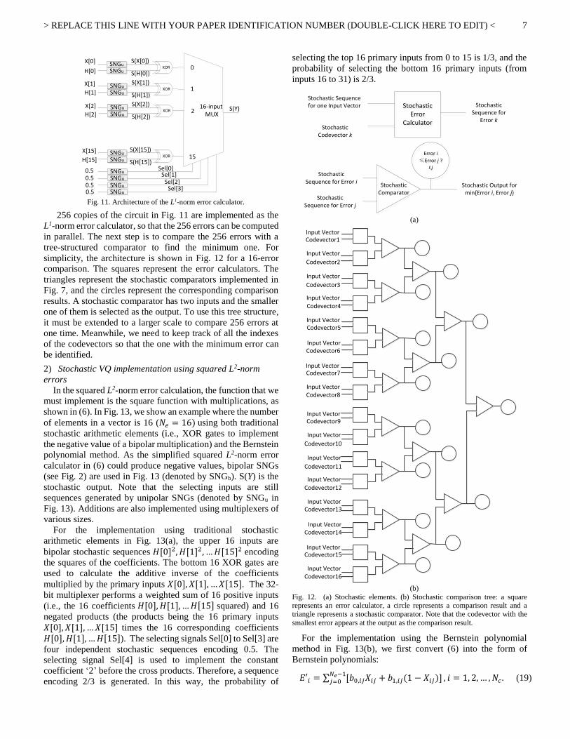
1) Stochastic VQ implementation using L1-norm errors

In the L1-norm error calculation, we need to implement (3).

In Fig. 11, an example is shown with 𝑁𝑒 =16 elements in a

vector. X[i] and H[i] represent the ith element in the input vector

and one of the 𝑁𝑐 = 256 codevectors, respectively. Both X[i]

and H[i] are encoded as stochastic sequences from their

previous 8-bit binary values for a grey-scale image. An RGB

color image can be treated by encoding the three colors

separately. This can be done using stochastic number generators

(SNGs), as described in the previous section, and the

computation is based on stochastic unipolar representations. In

Fig. 11, the label SNGu (see Fig. 2) is used to denote the

unipolar (regular) stochastic number generators. In our

stochastic VQ design, the stochastic error output S(Y) contains

the index embedded in binary format at the end of S(Y). This

binary value can be extracted later without requiring a counter.

The XOR gates are used to implement the absolute subtractions

in stochastic computing with correlated stochastic sequences,

where the correlated sequences attain the maximum overlap of

1’s [5]. This can be implemented by sharing the same LFSR for

SNGs at the inputs of the XOR gates. For the inputs of the

different XOR gates and selecting inputs of the multiplexer,

however, we generate sequences with different LFSRs and

initial seeds for SNGs in order to minimize the correlation.

Then the results are added up by the 16-input multiplexer whose

selecting signals Sel[0] to Sel[3] are four independent

stochastic sequences encoding 0.5.


7

16-input MUX

S(X[0])

Sel[0]

XOR

S(H[0])0

1

15

S(Y)

SNGuX[0]

H[0]

S(X[1])XOR

S(H[1])

SNGSNG

X[1]

H[1]

S(X[15])XOR

S(H[15])

SNGSNG

X[15]

H[15]

0.5 SNGu

SNGu

SNGu

SNGu

Sel[1]Sel[2]

Sel[3]

0.50.50.5

S(X[2])XOR

S(H[2])2

SNGSNG

X[2]

H[2]

SNGu

SNGu

SNGu

SNGu

SNGu

SNGu

SNGu

Fig. 11. Architecture of the L1-norm error calculator.

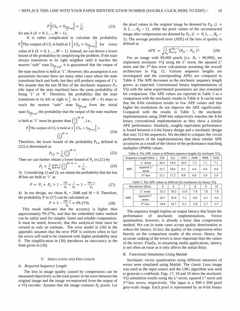
256 copies of the circuit in Fig. 11 are implemented as the

L1-norm error calculator, so that the 256 errors can be computed

in parallel. The next step is to compare the 256 errors with a

tree-structured comparator to find the minimum one. For

simplicity, the architecture is shown in Fig. 12 for a 16-error

comparison. The squares represent the error calculators. The

triangles represent the stochastic comparators implemented in

Fig. 7, and the circles represent the corresponding comparison

results. A stochastic comparator has two inputs and the smaller

one of them is selected as the output. To use this tree structure,

it must be extended to a larger scale to compare 256 errors at

one time. Meanwhile, we need to keep track of all the indexes

of the codevectors so that the one with the minimum error can

be identified.

2) Stochastic VQ implementation using squared L2-norm

errors

In the squared L2-norm error calculation, the function that we

must implement is the square function with multiplications, as

shown in (6). In Fig. 13, we show an example where the number

of elements in a vector is 16 (𝑁𝑒 = 16) using both traditional

stochastic arithmetic elements (i.e., XOR gates to implement

the negative value of a bipolar multiplication) and the Bernstein

polynomial method. As the simplified squared L2-norm error

calculator in (6) could produce negative values, bipolar SNGs

(see Fig. 2) are used in Fig. 13 (denoted by SNGb). S(Y) is the

stochastic output. Note that the selecting inputs are still

sequences generated by unipolar SNGs (denoted by SNGu in

Fig. 13). Additions are also implemented using multiplexers of

various sizes.

For the implementation using traditional stochastic

arithmetic elements in Fig. 13(a), the upper 16 inputs are

bipolar stochastic sequences 𝐻[0]2, 𝐻[1]2, … 𝐻[15]2 encoding

the squares of the coefficients. The bottom 16 XOR gates are

used to calculate the additive inverse of the coefficients

multiplied by the primary inputs 𝑋[0], 𝑋[1], … 𝑋[15]. The 32-

bit multiplexer performs a weighted sum of 16 positive inputs

(i.e., the 16 coefficients 𝐻[0], 𝐻[1], … 𝐻[15] squared) and 16

negated products (the products being the 16 primary inputs

𝑋[0], 𝑋[1], … 𝑋[15] times the 16 corresponding coefficients

𝐻[0], 𝐻[1], … 𝐻[15]). The selecting signals Sel[0] to Sel[3] are

four independent stochastic sequences encoding 0.5. The

selecting signal Sel[4] is used to implement the constant

coefficient ‘2’ before the cross products. Therefore, a sequence

encoding 2/3 is generated. In this way, the probability of

selecting the top 16 primary inputs from 0 to 15 is 1/3, and the

probability of selecting the bottom 16 primary inputs (from

inputs 16 to 31) is 2/3.

Stochastic Sequence for Error i

Stochastic Sequence for Error j

Stochastic Error

Calculator

Stochastic Error

Calculator

Error i

≤Error j ? i:j

Error i

≤Error j ? i:j

Stochastic Sequence for one Input Vector

Stochastic Codevector k

Stochastic Sequence for

Error k

Stochastic Output for min{Error i, Error j}

Stochastic Comparator

(a)

Input VectorCodevector1

Input Vector

Codevector2

Input Vector

Codevector3

Input Vector

Codevector4






Input Vector

Codevector10

Input Vector

Codevector11

Input Vector

Codevector12





(b)

Fig. 12. (a) Stochastic elements. (b) Stochastic comparison tree: a square represents an error calculator, a circle represents a comparison result and a

triangle represents a stochastic comparator. Note that the codevector with the

smallest error appears at the output as the comparison result.

For the implementation using the Bernstein polynomial

method in Fig. 13(b), we first convert (6) into the form of

Bernstein polynomials:

𝐸′𝑖 = ∑ [𝑏0,𝑖𝑗𝑋𝑖𝑗 + 𝑏1,𝑖𝑗(1 − 𝑋𝑖𝑗)]𝑁𝑒−1𝑗=0 , 𝑖 = 1, 2, … , 𝑁𝑐 . (19)


8

where 𝑏0,𝑖𝑗 = 𝐶𝑖𝑗2 − 2𝐶𝑖𝑗 and 𝑏1,𝑖𝑗 = 𝐶𝑖𝑗

2 are pre-computed

Bernstein coefficients. For every term indexed by j ( 𝑗 =0,1, 2, … , 𝑁𝑒 − 1 ) in (19), a 2-input multiplexer is needed.

There are a total of 16 two-input multiplexers (𝑁𝑒 = 16). A 16-

input multiplexer is then used to sum up the outputs of all the

two-input multiplexers. The new coefficients 𝑏0,𝑖𝑗 and 𝑏1,𝑖𝑗 are

encoded by independent bipolar stochastic number generators

(denoted by SNGb) while the primary inputs 𝑋𝑖𝑗 are encoded by

independent unipolar stochastic number generators (denoted by

SNGu). The selecting signals Sel[0] to Sel[3] are four

independent stochastic sequences encoding 0.5, which are also

unipolar stochastic sequences. The outputs of the squared L2-

norm error calculators in Fig. 13 are then passed on to the

parallel comparison tree in Fig. 12(b).

32-input MUXX[0]

X[1]

X[15]

H[0]

H[1]

H[15]

Sel[0]0.5 SNGu

SNGu

SNGu

SNGu

Sel[1]Sel[2]

Sel[3]

0.50.50.5

SNGuSel[4]

2/3

0

1

15

16

17

31

S(Y)

SNGb

SNGb

SNGb

SNGb

SNGb

SNGbXOR

XOR

XOR

SNGb

SNGb

SNGb

(a)

(b)

Fig. 13. Architecture of the squared L2-norm error calculator: (a) using

traditional stochastic arithmetic elements and (b) using the Bernstein polynomial method.

To compare the two implementations shown in Fig. 13, the

circuits for the squared error calculators were designed and

synthesized with the Synopsys Design Compiler tool [25]. The

resulting synthesis report provides the silicon area, the power

(including both static and dynamic powers) and the minimum

clock period (see Table 3). It is clear that the Bernstein

polynomial method shows slightly better performance, so the

implementation in Fig. 13(b) is selected as the squared L2-norm

error calculator. Although the advantage over the traditional

stochastic arithmetic elements is not so significant for the

squared L2-norm error calculation, the Bernstein polynomial

method becomes more favorable for the Lp-norm or pth-

law (𝑝 ≥ 3) error calculations. This is primarily because the

higher-order terms can be more efficiently implemented using

the Bernstein polynomial method in that fewer stochastic

number generators are required.

Table 3. Circuit performance of the squared error calculators using (a) traditional stochastic arithmetic elements and (b) the Bernstein polynomial

method (𝑁𝑒 = 16).

Area (um2) Power (uW) @ Min

Clock Period

Minimum Clock

Period (ns)

(a) (b) Ratio:

(a)/(b) (a) (b)

Ratio:

(a)/(b) (a) (b)

Ratio:

(a)/(b)

5.246 5.129 1.02 8.74 8.36 1.05 0.05 0.05 1

3) Stochastic VQ implementation using pth-law errors

As discussed above, the Bernstein polynomial method is

selected for error calculations of the pth-law (𝑝 ≥ 3) in (8) to

achieve efficiency. Based on the Bernstein polynomial

calculator in Fig. 8, the overall architecture of the pth-law error

calculator is shown in Fig. 14, where p=3 and 𝑁𝑒 = 16 in our

example. X[i] represents the ith element in the input vector. The

Bernstein coefficients b0[i], b1[i], b2[i] and b3[i] are calculated

using 𝑏𝑘 = ∑ (𝑘𝑗) (3

𝑗)⁄ ∙ 𝑎𝑘

𝑘

𝑗=0, where 𝑎𝑘 is the kth-order

coefficient of the error polynomial in (8) without the absolute

value function and k = 0, 1, 2, 3. For an input vector X with

𝑁𝑒 elements, the input X[i] (𝑖 = 0, 1, … , 𝑁𝑒 − 1 ) is always

positive as it is an 8-bit binary value encoding a grey scale pixel.

It is then converted into unipolar stochastic sequences. The

Bernstein coefficients can be positive or negative, so in Fig. 14

bipolar SNGs are used in the Bernstein polynomial calculators

(in Fig. 8). S(Y[i]) is the stochastic output of the absolute value

of the Bernstein polynomial for input X[i], where 0 ≤ 𝑖 ≤ 15

and the Bernstein polynomial has (p+1) terms for errors

measured by the pth-law. In general, a pth-law error is a sum of

𝑁𝑒 Bernstein polynomials. We therefore add up all the outputs

of 𝑁𝑒 Bernstein polynomials using an Ne-input multiplexer. The

output of the error calculator S(Y) in Fig. 14 is a stochastic

sequence to be compared with other errors in the stochastic

comparison tree shown in Fig. 12(b).

16-input MUX

Sel[0]

0

S(Y)

0.5 SNGu

SNGu

SNGu

SNGu

Sel[1]Sel[2]

Sel[3]

0.50.50.5

Bernstein Polynomial Calculator for X[0]

X[0]b0[0]b1[0]b2[0]b3[0]

1Bernstein Polynomial

Calculator for X[1]

X[1]b0[1]b1[1]b2[1]b3[1]

15Bernstein Polynomial Calculator for X[15]

X[15]b0[15]b1[15]b2[15]b3[15]

S(Y[0])

S(Y[1])

S(Y[15])

Fig. 14. Architecture of the pth-law error calculator for p=3 using the

Bernstein polynomial calculator in Fig. 8.

C. Index storage and delivery

A source vector is encoded by the index of the codevector


9

that produces the minimum error among all the calculated ones.

The comparison results come naturally as stochastic streams

that represent probabilities instead of deterministic Boolean

values. Therefore the stochastic streams have to be converted to

binary numbers by counters, which would add cost. To avoid

this problem, we can embed the index in the last few bits of the

stochastic sequence as a binary-encoded value, as shown in Fig.

15. The error of the kth codevector is labeled with index k.

Initially the error calculator is used to obtain the stochastic

sequence for the error of the kth codevector at the input port, and

then this stochastic error is labelled with index k. The last few

bits that are shaded in this stochastic error sequence in Fig. 15

represent the binary number k. The remaining bits represented

by the white squares in the bit stream are left unchanged in Fig.

15.

If the sequences are long enough, giving up the last few bits

will have little effect on the stochastic value. For most of the

codewords, the stochastic comparator will rapidly converge to

select one of the inputs as the output after an initial period of

instability. So we can rely on the index being delivered

correctly especially when the sequence is long enough. We

only prepare one counter at the last stage to extract the index

from the stochastic sequence. Registers for index storage and

counters used as the stochastic-to-binary converter for every

comparator are saved to reduce hardware cost. A shorter delay

also results as no extra time is needed to process the index,

which is extracted easily from the output bit stream.

Stochastic

Error

Calculator

Stochastic

Error

Calculator

Stochastic

Input Vectors

Stochastic

Codevector Ck

Remaining bits

are unchanged

Six-bit binary

index k

Stochastic Output for

Error denoted by Ek

Last six bits of the

error sequence to

be replaced with

the binary index k

Data Flow

Direction

To Comparators in

the Comparison Tree

Fig. 15. Embedding a 6-bit binary index into the stochastic error bit stream.

D. Error Analysis

A mathematical analysis is given to show the validity of the

index storage and delivery method. Assume that the last M bits

are used to store the index in an Ns-bit stochastic sequence (see

Fig. 16). The index of the smaller inputs between Px and Py must

be safely passed on through the stochastic comparator shown in

Fig. 7. This requires that the last M bits in the stochastic

sequence encoding Ps2 correctly indicate the result of

comparing stochastic numbers Px and Py. As Ps2 is the output of

the stochastic tanh function, we consider the state transition

diagram of the stochastic tanh function where 𝑁𝑠𝑡 is the number

of states in the FSM (see Fig. 5) and 𝑁𝑠 ≫ 𝑀 (see Fig. 16). Our

goal is to ensure with high probability that the last M bits in the

stochastic sequence encoding Ps2 are stable at ‘1’ (or ‘0’) for the

comparison result Px ≥ Py (or Px < Py). Now we calculate the

conditional probability P{Last M bits in Ps2 are all 1’s | Px ≥ Py}, which would be similar to calculating P{Last M bits in Ps2

are all 0’s | Px < Py }.

Stochastic Number (Ns bits)Stochastic Number (Ns bits)

Index storage (M bits)Index storage (M bits)

Fig. 16. The embedded index in a stochastic sequence.

To focus on the index embedded in the last M bits of a

stochastic sequence, we consider the state transitions after

(𝑁𝑠 − 𝑀) transitions in the diagram (see Fig. 5). The remaining

M states produce the last M bits of the stochastic sequence Ps2,

which selects the M-bit index of the smaller one between Px and

Py. Suppose that the current state is denoted by 𝐶𝑆𝑖, where i is

the storage bit index ( 𝑖 = 0, 1, … , 𝑀 − 1 ). We consider all

possible values of Ps1, which is the input of the tanh function,

to analyze the output Ps2. The computation steps are as follows.

1) It can be seen that 𝑆𝑁𝑠𝑡2

is the central state in the state

transition diagram in Fig. 5. 𝑆𝑁𝑠𝑡2

+𝑘 represents the kth state to the

right of 𝑆𝑁𝑠𝑡2

, where k (𝑘 = 0, 1, 2, …) is an integer index. When

𝑘 ≥ 𝑀, 𝑆𝑁𝑠𝑡2

+𝑘 is considered a “safe” initial state because the

next M transitions will remain in the right half of the state

transition diagram, regardless of the inputs (M-bit embedded

index shown in Fig. 16). Hence, if 𝐶𝑆0 = 𝑆𝑁𝑠𝑡2

+𝑘 and 𝑘 ≥ 𝑀,

the last M bits in Ps2 will be held at ‘1’. Assume that the two

errors Px and Py encoded by the stochastic sequences are evenly

distributed between 0 and 1. The probability that 𝐶𝑆0 = 𝑆𝑁𝑠𝑡2

+𝑘

and 𝑘 ≥ 𝑀 is

𝑃1 = 1 −2𝑀

𝑁𝑠+

𝑀2

𝑁𝑠2 > ( 1 −

2𝑀

𝑁s), (20)

which is proved in detail in the appendix.

2) If 𝐶𝑆0 = 𝑆𝑁𝑠𝑡2

+𝑘 and 0 ≤ 𝑘 < 𝑀 , the next state 𝐶𝑆𝑖 ( 𝑖 =

0, 1, … , 𝑀 − 1 ) will possibly cross the boundary from

outputting 1’s to outputting 0’s, so that it fails to hold the value

‘1’. Let the probability of not crossing the boundary be

𝑃2 = ∑ 𝑃2,𝑘𝑀−1𝑘=0 , (21)

where 𝑃2,𝑘 denotes the probability that the output of 𝐶𝑆𝑖 is held

at ‘1’ for any 𝑖 ∈ {0, 1, … , 𝑀 − 1} provided that 𝐶𝑆0 = 𝑆𝑁st2

+𝑘

(0 ≤ 𝑘 < 𝑀). By definition, 𝑃2,𝑘 can be obtained by

𝑃2,𝑘 = 𝑃 {𝐶𝑆0 = 𝑆𝑁st2

+𝑘} ×

P {The output of 𝐶𝑆𝑖 is held at 1|𝐶𝑆0 = 𝑆𝑁st2

+𝑘},

(22)

where 𝑘 = 0, 1, … , 𝑀 − 1. According to (37) in the appendix,

the probability that the initial state is 𝑆𝑁st2

+𝑘 can be calculated

as


10

𝑃 {𝐶𝑆0 = 𝑆𝑁st2

+𝑘} ≈

2

𝑁s, (23)

for any k (𝑘 = 0, 1, … , 𝑀 − 1).

It is rather complicated to calculate the probability

P {The output of 𝐶𝑆𝑖 is held at 1 | 𝐶𝑆0 = 𝑆𝑁st2

+𝑘} for every

value of k (𝑘 = 0, 1, … , 𝑀 − 1). Instead, we can derive a lower

bound of the probability by simplifying the problem. If the state

always transitions to its right neighbor until it reaches the

nearest “safe” state 𝑆𝑁𝑠𝑡2

+𝑀, it is guaranteed that the output of

the state machine is held at ‘1’. However, this assumption is too

pessimistic because there are many other cases where the state

transitions back and forth, but they still produce outputs of 1’s.

We assume that the last M bits of the stochastic sequence Ps1

(the input of the state machine) have the same probability of

being ‘1’ or ‘0’. Therefore, the probability that the state

transitions to its left or right is 1

2. As it takes (𝑀 − 𝑘) steps to

reach the nearest “safe” state SNst2

+M from the initial

state 𝑆𝑁st2

+𝑘, the probability that the output of the state machine

is held at ‘1’ must be greater than (1

2)

𝑀−𝑘

, i.e.,

P {The output of 𝐶𝑆𝑖 is held at 1 | 𝐶𝑆0 = 𝑆𝑁st2

+𝑘} >

(1

2)

𝑀−𝑘.

(24)

Therefore, the lower bound of the probability 𝑃2,𝑘 defined in

(22) is determined as

𝑃2,𝑘 >2

𝑁s(

1

2)

𝑀−𝑘

. (25)

Then we can further obtain a lower bound of 𝑃2 in (21) by

𝑃2 >2

𝑁s∑ (

1

2)

𝑀−𝑘−1𝑀−1𝑘=0 ≈

1

𝑁s . (26)

3) Considering 1) and 2), we obtain the probability that the last

M bits are held at ‘1’ as

𝑃 = 𝑃1 + 𝑃2 > 1 −2𝑀

𝑁s+

1

𝑁s= 1 −

2𝑀−1

𝑁s (27)

4) In our design, we chose 𝑁𝑠 = 2048 and M = 8. Therefore,

the probability P in (27) can be calculated as

𝑃 > 1 −2𝑀−1

𝑁s≈ 99.27% (28)

This result indicates that the accuracy is higher than

approximately 99.27%, and that the embedded index method

can be safely used for simpler, faster and reliable computation.

It must be noted, however, that this analytical limit must be

viewed as only an estimate. The error model in (30) in the

appendix assumes that the error PDF is uniform when in fact

the errors will tend to be clustered with higher probability near

0. The simplification in (30) introduces an inaccuracy in the

limit given in (28).

V. SIMULATION AND DISCUSSION

A. Required Sequence Length

The loss in image quality caused by compression can be

measured objectively as the total power in the error between the

original image and the image reconstructed from the output of

a VQ encoder. Assume that the image contains Np pixels. Let

the pixel values in the original image be denoted by 𝑃𝑂𝑖 (𝑖 = 0, 1, … , 𝑁𝑝 − 1), while the pixel values of the reconstructed

image after compression are denoted by 𝑃𝐶𝑖 (𝑖 = 0, 1, … , 𝑁𝑝 −

1). The average penalized error (APE) of the loss of quality is

defined as

𝐴𝑃𝐸 = √1

𝑁𝑝∑ (𝑃𝑂𝑖 – 𝑃𝐶𝑖 )2𝑁𝑝−1

𝑖=0. (29)

For an image with 90,000 pixels (i.e. Np = 90,000), we

implement stochastic VQ using the L1 norm, the squared L2

norm and the 3rd-law error calculations assuming the overall

architecture in Fig. 12. Various sequence lengths are

investigated and the corresponding APEs are compared in

Table 4. The APE decreases as the stochastic sequence length

grows, as expected. Conventional binary implementations of

VQ with the same experimental parameters are also simulated

for comparison. The APE values are reported in Table 5 as a

comparison with the stochastic results in Table 4. It can be seen

that the 8-bit resolution results in low APE values and that

higher bit resolutions do not improve the APE significantly.

Compared with the results in Table 5, the stochastic

implementation using 2048 bits subjectively matches the 8-bit

binary conventional implementation as they show a similar

APE performance. Similarly, roughly equivalent performance

is found between a 6-bit binary design and a stochastic design

that uses 512-bit sequences. We decided to compare the circuit

performances of the implementations that show similar APE

accuracies as a result of the choice of the performance matching

multiplier (PMM) values.

Table 4. The APE values at different sequence lengths for stochastic VQ.

Sequence Length (bits) 256 512 1024 2048 4096 9192

APE

L1 norm 30.4 19.9 10.9 7.3 7.1 7.1

squared L2

norm 25.7 18.6 9.5 6.0 6.0 6.0

3rd-law 25.1 17.2 8.8 6.0 5.9 5.9

Table 5. The APE values at different bit resolutions for binary VQ.

Resolution (Bits) 4 6 7 8 9 10

APE

L1 norm 33.1 18.3 11.0 7.8 7.8 7.8

squared L2

norm 26.7 16.9 7.2 6.0 6.1 6.0

3rd-law 24.6 14.7 6.2 5.8 5.7 5.7

The sequence length implies an output latency that limits the

performance of stochastic implementations. Vector

quantization, however, is already a lossy data compression

method. We can in some cases accept quality deterioration to

reduce the latency. In fact, the quality of the compression relies

heavily on the comparison results of the errors. Hence, the

accurate ranking of the errors is more important than the values

of the errors. Finally, in streaming media applications, latency

is not often an issue as it only affects the initial delay.

B. Functional Simulation Using Matlab

Stochastic vector quantization using different measures of

errors were simulated using Matlab. The classic Lena image

was used as the input source and the LBG algorithm was used

to generate a codebook. Figs. 17, 18 and 19 show the stochastic

VQ simulation results using the L1-norm, squared L2-norm and

3rd-law errors, respectively. The input is a 300 × 300 pixel

grey-scale image. Each pixel is represented by an 8-bit binary


11

number. After using stochastic vector quantization to compress

the original image, the image is re-constructed using codebook

look-up and displayed for visual quality assessment. The image

has 5625 input vectors, and each vector comprises 16 unsigned

8-bit pixel values. We use 2048 bits in a stochastic

representation, so it takes 2048 clock cycles to finish one round

of calculation. To encode the 5625 input vectors in a fully-

parallel architecture, a total of 5625 independent processor units

are required and each unit includes 256 error calculators and a

256-input comparison tree.

Fig. 17. The progressive improvement of image quality using L1-norm

stochastic VQ after 256, 512, 1024 and 2048 clock cycles.

Fig. 18. The progressive improvement of image quality using squared L2-norm stochastic VQ after 256, 512, 1024 and 2048 clock cycles.

Fig. 19. The progressive improvement of image quality using the 3rd-law

stochastic VQ after 256, 512, 1024 and 2048 clock cycles.

The output images in Figs. 17, 18 and 19 illustrate the

progressive quality feature of stochastic computing. The

reconstructed image after stochastic compression for the 256th,

512th, 1024th and 2048th clock cycles are shown for the three

error measures. However the reconstructed output images are

vague and only show a rough outline of the original image after

compression using 256 clock cycles. The reconstructed image

becomes a clearer and more accurate reproduction as the

stochastic encoding time increases. The stochastic

representation of 2048 bits can be generated by an 11-bit LFSR

in a Matlab function. Note that because the stochastic sequences

repeat every 2048 cycles, the image quality will not improve for

additional clock cycles beyond 2048.

C. Circuit Performances

Following the results in Tables 4 and 5, we compared (a) an

8-bit binary implementation with the stochastic implementation

using 2048-bit sequences, (b) a 7-bit binary implementation

with the stochastic implementation using 1024-bit sequences

and (c) a lower quality processing implementation using the 6-

bit binary and the 512-bit stochastic designs. The hardware area,

power consumption and delay comparisons are shown in Tables

6, 7 and 8 for L1-norm, squared L2-norm and 3rd-law

implementations, respectively. The stochastic circuits are built

according to the architecture in Fig. 12(b). The designs of the

error calculators are shown in Figs. 11, 13 and 14. By using the

Synopsys design compiler, which automatically maximized the

data throughputs by introducing pipeline registers in both the

stochastic and binary VQ designs, we obtained the fastest clock

that still meets the timing requirements. Then the power

consumption and silicon area were obtained for the fastest clock

frequency. Note that the auxiliary circuits such as stochastic

number generators (implemented by LFSRs) and counters are

all included.

As shown in Tables 6, 7 and 8, the stochastic circuits have

significantly lower hardware cost. Stochastic implementations

only cost roughly 1% of the hardware of binary

implementations. This also leads to savings in power

consumption. The time required for an encoding operation is

also an important measurement to calculate the total energy,

and it is determined by the product of the clock period and the

stochastic sequence length. Because the structure of stochastic

circuits is simpler, a shorter critical path delay is expected. This

is reflected in the columns showing that the minimum stochastic

clock periods are smaller than the minimum binary clock

periods.

We used the energy per operation (EPO) and the throughput

per area (TPA) as two generic metrics. The EPO is defined in

the binary case to be the energy consumed in one binary clock

period; in the stochastic case, the EPO is the energy consumed

over one stochastic sequence. We are assuming here that the

processing pipeline is full and we are ignoring the fixed pipeline

latency. The TPA is defined to be the number of input vectors

compressed per unit area. In the stochastic case the TPA is

reduced by the length of the stochastic sequence. In Table 6 for

the L1-norm, the stochastic approach shows significant

advantages over the binary approach in terms of the area cost,

power consumption and delay. When long sequences such as

2048 bits are considered, the ratio of stochastic over binary

energy per operation is about 5.38, and the ratio of the

throughputs per area is approximately 0.38. Therefore, the

stochastic approach using 2048-bit sequences underperforms

the conventional binary approach using 8-bit resolution.

However, if some loss in quality is acceptable in the application,

the stochastic implementation using 512-bit sequences shows

only 2.38 times the energy cost per operation and 2.56 times

throughput per area in only 1.5% the total area compared to a

6-bit binary implementation. It can be seen that the stochastic

implementation using 1024-bit sequences shows similar

performance compared to the 7-bit binary implementation in

terms of TPA. The stochastic VQ is thus not competitive for 7-

bit or higher bit resolutions in terms of the TPA performance.


12

Table 6. Circuit performance of L1-norm vector quantization with three

compression qualities: (a) 8-bit binary (B) vs. 2048-bit stochastic (S), (b) 7-bit

binary (B) vs. 1024-bit stochastic (S) and (c) 6-bit binary (B) vs. 512-bit

stochastic (S).

Area (𝜇𝑚2) Power (mW) @ Min

Clock Period

Minimum Clock

Period (ns)

B S Ratio:

S/B B S

Ratio:

S/B B S

Ratio:

S/B

(a) 93294 1358 0.015 107.56 3.22 0.03 2.28 0.20 0.09

(b) 86231 1003 0.012 81.30 2.86 0.04 2.26 0.20 0.09

(c) 79177 641 0.008 50.09 2.47 0.05 2.23 0.21 0.09

Energy per Operation

(pJ/Operation)

Throughput per Area

(1/(𝜇𝑚2 ∙ 𝑠))

Required Sequence

Length (bits)

B S Ratio:

S/B B S

Ratio:

S/B B S

Ratio:

S/B

(a) 245 1319 5.38 4701 1798 0.38 N/A 2048 N/A

(b) 184 586 3.19 5131 4868 0.95 N/A 1024 N/A

(c) 112 266 2.38 5664 14510 2.56 N/A 512 N/A

In Tables 7 and 8, the stochastic VQ implementations for the

squared L2-norm and the 3rd-law errors are compared with the

conventional binary implementations. In general, the squared

L2-norm and the 3rd-law implementations use more hardware

and consume more energy as the computational complexity

increases from the L1-norm implementation. However, the

implementation areas for the stochastic implementations are

still less than 1.5% of the binary designs. The TPAs of the 3rd-

law VQ implementations are much smaller than those of L1-

norm and squared L2-norm VQ implementations. However, the

squared L2-norm and the 3rd-law benefit from more accurate

results compared with the L1 norm. For the same stochastic

sequence length, the reconstructed images using the squared L2-

norm and the 3rd-law have higher fidelity as they show smaller

average penalized error (APE) than that using the L1 norm, as

shown in Table 4. The 3rd-law VQ takes advantage of the

Bernstein polynomial method to build the error calculator based

on high order polynomials. It shows the best compression

quality compared with the other two implementations.

Table 7. Circuit performance of squared L2-norm vector quantization with

three compression qualities: (a) 8-bit binary (B) vs. 2048-bit stochastic (S), (b)

7-bit binary (B) vs. 1024-bit stochastic (S) and (c) 6-bit binary (B) vs. 512-bit stochastic (S).


Clock Period

Minimum Clock

Period (ns)

B S Ratio:

S/B B S

Ratio:

S/B B S

Ratio:

S/B

(a) 113847 1588 0.014 61.48 3.17 0.052 2.29 0.21 0.09

(b) 99631 1264 0.013 56.30 2.79 0.050 2.26 0.20 0.09

(c) 89992 972 0.011 50.09 2.39 0.048 2.23 0.20 0.09


(pJ/Operation)

Throughput per Area

(1/(𝜇𝑚2 ∙ 𝑠))

Required Sequence

Length (bits)

B S Ratio:

S/B B S

Ratio:

S/B B S

Ratio:

S/B

(a) 141 1363 9.68 3836 1464 0.38 N/A 2048 N/A

(b) 127 571 4.49 4441 3863 0.87 N/A 1024 N/A

(c) 112 245 2.19 4983 10047 2.02 N/A 512 N/A

Table 8. Circuit performance of 3rd-law vector quantization with three

compression qualities: (a) 8-bit binary (B) vs. 2048-bit stochastic (S), (b) 7-bit

binary (B) vs. 1024-bit stochastic (S) and (c) 6-bit binary (B) vs. 512-bit

stochastic (S).


Clock Period

Minimum Clock

Period (ns)

B S Ratio:

S/B B S

Ratio:

S/B B S

Ratio:

S/B

(a) 256261 3772 0.014 183.2 12.86 0.07 4.43 0.55 0.12

(b) 247439 3481 0.014 179.6 11.71 0.07 4.41 0.55 0.09

(c) 238261 3251 0.013 175.7 10.72 0.06 4.38 0.54 0.12


(pJ/Operation)

Throughput per Area

(1/(𝜇𝑚2 ∙ 𝑠))

Required Sequence

Length (bits)

B S Ratio:

S/B B S

Ratio:

S/B B S

Ratio:

S/B

(a) 812 14486 17.85 881 235 0.27 N/A 2048 N/A

(b) 792 6595 8.33 917 510 0.56 N/A 1024 N/A

(c) 770 2964 3.85 958 1113 1.16 N/A 512 N/A

When high-quality (8-bit binary and 2048-bit stochastic) VQ

implementations are considered, the EPO ratios of the

stochastic implementation over conventional binary

implementation are 9.68 and 17.85 for the squared L2-norm and

the 3rd-law errors, respectively. For lower-quality (6-bit binary

and 512-bit stochastic) VQ implementations, the EPO ratios

become 2.19 and 3.85 for the squared L2-norm and the 3rd-law

errors, respectively. With respective to the EPO, therefore, the

stochastic implementations are not competitive due to the

required long sequences.

For high-quality VQ compressions (using 2048-bit stochastic

and 8-bit conventional binary implementations), the stochastic

implementations are not advantageous over the conventional

binary implementations in terms of TPA. When a lower-quality

compression is acceptable (using 512-bit stochastic and 6-bit

conventional binary implementations), however, the TPA ratios

of the stochastic implementation over the conventional binary

implementation are 2.02 and 1.16 for the squared L2-norm and

the 3rd-law errors, respectively. The stochastic approach using

shorter sequences loses some accuracy but saves more in terms

of hardware cost and power consumption. By comparing the

1024-bit stochastic and 7-bit conventional binary VQ

implementations, we see that the stochastic approach could be

competitive for resolutions below 7 bits in terms of TPA.

The stochastic sequence length is a parameter that has a

maximum value for any given system design. It is determined

by the shortest repetition period among all the SNGs. The

shortest period must be chosen to amply satisfy the needs of the

application as reflected by the minimum acceptable subjective

reconstruction quality (e.g., image quality as perceived by

human users) and/or the minimum acceptable objective APE.

Once the shortest period has been synthesized into the system

design, a global stochastic bit counter can be used to further

trim back the sequence length at run time to provide a simple

control over the trade-off between compression time,

compression energy and reconstruction quality.

Stochastic VQ has the flexibility to easily adapt to poor

communication channels where lower compression quality is

preferred. Using L1 norm, for example, we can compress two

input images using the 2048-bit stochastic VQ implementation

and achieve the same compression quality as the 1024-bit

stochastic VQ implementation. In this way, only the 2048-bit

stochastic VQ implementation is needed instead of two copies


13

of the 1024-bit stochastic VQ circuit, further saving 32.3% of

the hardware area.

VI. CONCLUSIONS

The objective of the reported research was to clarify the

potential benefits of stochastic vector quantization versus

conventional binary VQ. In the image compression application

of VQ we determined the minimum stochastic sequence lengths

and binary resolutions that are required to produce equivalent

reconstruction accuracy in both the stochastic and binary VQ

compressors. We evaluated the various designs according

generic figures of merit including minimum clock period with

optimal pipelining, energy per operation and throughput per

area.

In this paper, stochastic circuits are designed to implement

the L1-norm, squared L2-norm and pth-law (𝑝 = 3 is used as an

example)-based vector quantization (VQ). Finite state machine-

based stochastic arithmetic elements and the Bernstein

polynomials are used to build error calculators and stochastic

comparison trees. By embedding the codevector indexes into

the last few bits of the stochastic error sequences, costly

counters are saved to reduce hardware cost. Various sequence

lengths are considered in the stochastic vector quantization and

the compression quality was assessed using average penalized

error (APE) for a grey-scale image.

Implementations using a codebook of 256 codevectors with

similar compression qualities are then compared with respect to

APE: (a) an 8-bit binary implementation with the stochastic

implementation using 2048-bit sequences, (b) a 7-bit binary

implementation with the stochastic implementation using 1024-

bit sequences and (c) a lower quality processing

implementation using the 6-bit binary and the 512-bit stochastic

designs. Due to the compact stochastic arithmetic elements and

an efficient index storage approach, the area advantage of the

stochastic VQ implementations is significant. The

implementation areas for the stochastic circuits are no more

than 1.5% of the fully parallel binary implementations. Our

results show that the stochastic VQ underperforms the

conventional binary VQ in terms of energy per operation.

However, the stochastic VQ can be efficient in terms of

throughput per area (TPA) when the implementation (c) with

an acceptable lower quality is considered. For the three error

measures, the TPA of the 512-bit stochastic implementation is

shown to be 1.16, 2.02 and 2.56 times as large as that of the 6-

bit binary implementations with a similar compression quality.

It can be seen that for resolutions of 7 bits and above, the

stochastic implementations underperform the corresponding

binary implementations in terms of TPA. However, the lower

quality of the reconstructed images is in fact a greater challenge

for stochastic VQ, as illustrated in Figures 18 and 19.

Successful applications of stochastic VQ must be justified on

the basis of its superior system-level error and fault tolerance

properties, along with a TPA that is at least comparable with

that of binary VQ. For example, from Table 6, 2048-bit

stochastic VQ has 38% of the TPA of 8-bit binary VQ, offering

equivalent image quality with superior system-level error and

fault tolerance.

Applications that could benefit from stochastic VQ must

value its superior system-level error and fault tolerance. High-

radiation environments might be one suitable application,

where real-time image data or sensor measurements must be

compressed and either stored in the sensor or communicated to

the outside despite conditions that render conventional digital

systems inoperable.

The inherent progressive quality, of the stochastic VQ design,

with its simply-controlled scalability, might be attractive in

some applications. An example might be a large network of

security cameras, where most of the time, the pixel accuracy

can be quite low. But periodically, or in response to a raised

alarm, the accuracy of some video frames can be increased by

using a longer stochastic sequence. This variable resolution

feature could be elegantly handled with a single stochastic VQ

circuit design in each camera.

APPENDIX

In this appendix, we prove Equation (20) by calculating the

probability P1 that 𝐶𝑆0 = 𝑆𝑁𝑠2

+𝑘 and 𝑘 ≥ 𝑀 (see Figs. 5 and

16). Equation (23) can be proved using the same method.

Assume that the stochastic errors 𝐸𝑖 ( 𝑖 = 1, 2, … , 𝑁𝑐 ) are

evenly distributed between 0 and 1. The probability density

function (PDF) of 𝐸𝑖 is

𝑓(𝑒) = {1, if 0 ≤ 𝑒 ≤ 1;0, 𝑜𝑡ℎ𝑒𝑟𝑤𝑖𝑠𝑒.

(30)

Let 𝐷𝑖,𝑗 denote the difference between two independent

errors 𝐸𝑖 ≥ 𝐸𝑗, where 𝑖, 𝑗 ∈ {1, 2, … , 𝑁𝑐} and 𝑖 ≠ 𝑗.

𝐷𝑖,𝑗 = 𝐸𝑖 − 𝐸𝑗 . (31)

Then the problem becomes to determine the probability

that 𝐷𝑖,𝑗 ≥ 𝑀

𝑁𝑠, where M is the number of storage bits and Ns is

the total length of a stochastic sequence. To solve this problem,

we consider the distribution of 𝐷𝑖,𝑗. The PDF of 𝐷𝑖,𝑗 is given

by the convolution of the PDFs of 𝐸𝑖 and (−𝐸𝑗) [26], i.e.,

𝑓 𝐷𝑖,𝑗(𝑥) = 𝑓𝐸𝑖+(−𝐸𝑗)(𝑥) = ∫ 𝑓(𝑒, 𝑥 − 𝑒)𝑑𝑒

∞

−∞=

∫ 𝑓𝐸𝑖(𝑒)𝑓−𝐸𝑗

(𝑥 − 𝑒)𝑑𝑒∞

−∞.

(32)

According to (30), we have

𝑓𝐸𝑖(𝑒) = {

1, if 0 ≤ 𝑒 ≤ 1;0, 𝑜𝑡ℎ𝑒𝑟𝑤𝑖𝑠𝑒.

(33)

𝑓−𝐸𝑗(𝑒) = {

1, if − 1 ≤ 𝑒 ≤ 0;0, 𝑜𝑡ℎ𝑒𝑟𝑤𝑖𝑠𝑒.

(34)

Substituting (33) and (34) into (32), the PDF of 𝐷𝑖,𝑗 is given by

𝑓 𝐷𝑖,𝑗(𝑥) = {

𝑥 + 1, if − 1 ≤ 𝑥 ≤ 0;1 − 𝑥, if 0 < 𝑥 ≤ 1;0, 𝑜𝑡ℎ𝑒𝑟𝑤𝑖𝑠𝑒.

(35)

Therefore, 𝑃1 is given by

𝑃1 =𝑃{𝐷𝑖,𝑗≥

𝑀

𝑁𝑠}

𝑃{𝐷𝑖,𝑗≥ 0}=

∫ 𝑓 𝐷𝑖,𝑗(𝑥)𝑑𝑥

1 𝑀/𝑁𝑠

∫ 𝑓 𝐷𝑖,𝑗(𝑥)𝑑𝑥

10

= 1 −2𝑀

𝑁𝑠+

𝑀2

𝑁𝑠2 , (36)

which is the same as (20).

Similarly, we can calculate 𝑃2,𝑘 as

𝑃2,𝑘 = 𝑃 {𝐶𝑆0 = 𝑆𝑁st2

+𝑘} =

𝑃{𝐷𝑖,𝑗≥ 𝑘

𝑁𝑠}

𝑃{𝐷𝑖,𝑗≥ 0}−

𝑃{𝐷𝑖,𝑗≥ 𝑘+1

𝑁𝑠}

𝑃{𝐷𝑖,𝑗≥ 0}=

(1 −2𝑘

𝑁𝑠+

𝑘2

𝑁𝑠2) − (1 −

2(𝑘+1)

𝑁𝑠+

𝑀(𝑘+1)2

𝑁𝑠2 ) ≈

2

𝑁𝑠,

(37)

which is the same as (23).


14

REFERENCES

[1] B. Gaines, “Stochastic computing systems,” in Advances in Information Systems Science, Springer, 1969, pp. 37-172.

[2] A. Alaghi and J. P. Hayes, “Survey of stochastic computing,” ACM

Transactions on Embedded Computing Systems (TECS), vol. 12, no. 2, p. 92, 2013.

[3] B.D. Brown, and H.C. Card. "Stochastic neural computation. I.

Computational elements." IEEE Transactions on Computers, vol. 50, no. 9 (2001): 891-905.

[4] B.D. Brown, and H.C. Card. "Stochastic neural computation. II. Soft

competitive learning." IEEE Transactions on Computers, vol. 50, no. 9 (2001): 906-920.

[5] A. Alaghi, C. Li and J. P. Hayes. "Stochastic circuits for real-time image-

processing applications." In Proc. of the 50th Annual Design Automation Conf., p. 136:1-6. ACM, 2013.

[6] W. Qian and M. D. Riedel. "The synthesis of robust polynomial arithmetic

with stochastic logic." In Design Automation Conference, pp. 648-653. IEEE, 2008.

[7] W. Qian, X. Li, M.D. Riedel, K. Bazargan, and D.J. Lilja. "An

architecture for fault-tolerant computation with stochastic logic." IEEE Transactions on Computers, vol. 60, no. 1 (2011): 93-105.

[8] H. Chen and J. Han, “Stochastic computational models for accurate reliability evaluation of logic circuits,” in GLSVLSI’10, Proceedings of

the 20th IEEE/ACM Great Lakes Symposium on VLSI, Providence, Rhode

Island, USA, pp. 61–66, 2010. [9] J. Han, H. Chen, J. Liang, P. Zhu, Z. Yang and F. Lombardi, “A Stochastic

Computational Approach for Accurate and Efficient Reliability

Evaluation,” IEEE Transactions on Computers, vol. 63, no. 6, pp. 1336 - 1350, 2014..

[10] P. Zhu, J. Han, L. Liu and M.J. Zuo, “A Stochastic Approach for the

Analysis of Fault Trees with Priority AND Gates,” in IEEE Trans. on Reliability, vol. 63, no. 2, pp. 480 - 494, 2014.

[11] P. Zhu, J. Han, L. Liu and F. Lombardi, “A Stochastic Approach for the

Analysis of Dynamic Fault Trees with Spare Gates under Probabilistic Common Cause Failures,” IEEE Trans. on Reliability, 2015.

[12] J.F. Keane, and L.E. Atlas. "Impulses and stochastic arithmetic for signal

processing." In Acoustics, Speech, and Signal Processing, Proceedings.(ICASSP'01). IEEE International Conference on, vol. 2, pp.

1257-1260. IEEE, 2001.

[13] V.C. Gaudet, and A.C. Rapley. "Iterative decoding using stochastic

computation." Electronics Letters, vol. 39, no. 3 (2003): 299-301.

[14] W.J. Gross, V.C. Gaudet, and A. Milner. "Stochastic implementation of

LDPC decoders." In Signals, Systems and Computers, 2005. Conference Record of the Thirty-Ninth Asilomar Conference on, pp. 713-717. IEEE,

2005.

[15] Y. Chang and K. K. Parhi, "Architectures for digital filters using stochastic computing." 2013 IEEE International Conference on,

Acoustics, Speech and Signal Processing (ICASSP), pp. 2697-2701.

[16] R. Wang, J. Han, B.F. Cockburn, D.G. Elliott, "Design, evaluation and fault-tolerance analysis of stochastic FIR filters," Microelectronics

Reliability, 2015.

[17] P. Li and D. J. Lilja, "Using stochastic computing to implement digital image processing algorithms." Proc. 29th Int. Conf. on Computer Design,

IEEE, 2011.

[18] Li, Peng, David J. Lilja, Wei Qian, Marc D. Riedel, and Kia Bazargan. "Logical computation on stochastic bit streams with linear finite-state

machines." IEEE Transactions on Computers, vol. 63, no. 6 (2014): 1474-

1486. [19] P. Li, D. J. Lilja, W. Qian, K. Bazargan, and M. D. Riedel, “Computation

on stochastic bit streams digital image processing case studies," IEEE

Trans. on Very Large Scale Integration (VLSI) Systems, vol. 22, no. 3, pp. 449-462, 2014.

[20] Y. Linde, A. Buzo and R. M. Gray, "An algorithm for vector quantizer

design." IEEE Trans. on Communications, vol. 28, no.1, pp.84-95, 1980. [21] F. K. Soong, A. E. Rosenberg, B. Juang, and L. R. Rabiner, "Report: A

vector quantization approach to speaker recognition." AT&T Technical

Journal, vol. 66, no. 2, pp. 14-26, 1987. [22] N. M. Nasrabadi and R. A. King, "Image coding using vector quantization:

A review." IEEE Trans. on Communications, vol. 36, no.8, pp 957-971,

1988. [23] R. Wang, J. Han, B. Cockburn and D. Elliott, “Stochastic Circuit Design

and Performance Evaluation of Vector Quantization,” in Proc. IEEE ASAP

2015, IEEE 26th International Conference on Application-specific

Systems, Architectures and Processors, Toronto, Canada, July 27 - 29,

2015.

[24] J. Makhoul, S. Roucos and H. Gish. "Vector quantization in speech

coding." Proc. IEEE, vol. 73, no. 11, pp. 1551-1588, 1985.

[25] D. W. Knapp, Behavioral synthesis: Digital system design using the

Synopsys behavioral compiler, Prentice-Hall, Inc., 1996. [26] D. D. Wackerly and R. L. Scheaffer, “Multivariate Probability

Distributions.” in Mathematical Statistics with Applications, 6th ed.

Duxbury, 2002, ch. 5, pp. 223–295.


15

Ran Wang was born in Anyang, China,

in 1988. He received the B.Eng. degree

in the School of Electronic Engineering

and Computer Science from Peking

University, Beijing, China, in 2012, and

the M.Sc. degree from the Department of

Electrical and Computer Engineering,

University of Alberta, Edmonton, AB,

Canada.

His research interests include stochastic circuit design,

system fault-tolerance analysis and their applications in image

processing. He is also interested in PVT variation analysis to

facilitate custom IC design.

Jie Han (S’02–M’05) received the

B.Sc. degree in electronic engineering

from Tsinghua University, Beijing,

China, in 1999 and the Ph.D. degree

from Delft University of Technology,

The Netherlands, in 2004. He is

currently an associate professor in the

Department of Electrical and Computer

Engineering at the University of

Alberta, Edmonton, AB, Canada.

His research interests include reliability and fault tolerance,

nanoelectronic circuits and systems, and novel computational

models for nanoscale and biological applications.

Dr. Han and coauthors have won the Best Paper Award at

IEEE/ACM International Symposium on Nanoscale

Architectures 2015 (NanoArch'15) and a Best Paper

Nomination at the 25th IEEE/ACM Great Lakes Symposium on

VLSI (GLSVLSI’15). His work was recognized by the 125th

anniversary issue of Science, for developing a theory of fault-

tolerant nanocircuits. He was also nominated for the 2006

Christiaan Huygens Prize of Science by the Royal Dutch

Academy of Science (Koninklijke Nederlandse Akademie van

Wetenschappen (KNAW) Christiaan Huygens

Wetenschapsprijs). Dr. Han is serving as a guest editor for the

Special Issue on Approximate and Stochastic Computing

Circuits, Systems and Algorithms, IEEE Transactions on

Emerging Topics in Computing, 2016. He is also serving as a

Technical Program Chair in the IEEE/ACM Great Lakes

Symposium on VLSI (GLSVLSI 2016). He served as a General

Chair and a Technical Program Chair in the IEEE International

Symposium on Defect and Fault Tolerance in VLSI and

Nanotechnology Systems (DFT) 2013 and 2012, respectively.

He also served as a Technical Program Committee member in

the Design, Automation & Test in Europe Conference (DATE

2014, 2015 and 2016), DFT 2011-2015, and several other

international conferences and workshops.

Bruce F. Cockburn (S'86—M'95)

completed the B.Sc. degree in

engineering physics in 1981 from

Queen's University at Kingston, Canada.

In 1985 and 1990 he completed M.Math.

and Ph.D. degrees, respectively, in

computer science from the University of

Waterloo.

He is a Professor in the Department

of Electrical and Computer Engineering at the University of

Alberta in Edmonton, Canada. From 1981 to 1983 he worked

as a Test Engineer and Software Designer at Mitel Corporation,

Kanata, ON, Canada. In 2001 he was a visiting engineer at

Agilent Technologies in Santa Clara. Over 2014-15, he was a

sabbatical visitor at the University of British Columbia in

Vancouver. His research interests include VLSI design and

test, built-in self-repair and self-test, application-specific

hardware accelerator architectures, applications of field-

programmable gate arrays, and genetic data processing.

Dr. Cockburn is a member of the IEEE Computer Society,

the IEEE Communications Society, the IEEE Solid-State

Circuits Society, the IEEE Signal Processing Society, and the

Association for Computing Machinery. He is a registered

Professional Engineer in the Province of Alberta, Canada.

Duncan G. Elliott (M’97) received his

B.A.Sc. in Engineering Science and his

masters and doctorate degrees in

Electrical and Computer Engineering

from the University of Toronto.

He is a Professor in the Department

of Electrical and Computer Engineering

at the University of Alberta, Edmonton,

Canada. Previously, he has worked at

Nortel in data communications, at

MOSAID Technologies as a DRAM designer, and at IBM

Microelectronics as a contractor in application-specific

memory design. His research interests include merged

microfluidic-microelectronic systems, information processing

architectures, RF & communications circuits and unmanned

aircraft systems.

Professor Elliott was the 2001 winner of the Colton Medal

in microelectronics for his work on Computational RAM,

which has been commercialized. He is a member of the IEEE

and ACM.

stochastic circuit design and performance evaluation of...

Documents