stochastic and optimal aggregation of electric vehicles...

Aalborg University Department of Energy Technology

Stochastic and Optimal Aggregation of Electric

Vehicles in Smart Distribution Grids

Master Thesis

Zheyuan Hu

2013/5/30

Cover image is from Sustainable Building Solutions (SBS), a division of Travis Perkins plc.

Title: Stochastic and Optimal Aggregation of Electric Vehicles in Smart Distribution Grids Semester: 9th ─ 10th

Semester theme: Master’s Thesis Project period: 1st of September 2012 ─ 30th of May 2013 ECTS: 50 Supervisor: Jayakrishnan R Pillai Project group: WPS4-1050 _____________________________________ [Zheyuan Hu] _____________________________________ _____________________________________ _____________________________________ _____________________________________ _____________________________________

Copies: [3] Pages, total: [110] Appendix: [16] Supplements: [1 CD] By signing this document, each member of the group confirms that all group members have participated in the project work, and thereby all members are collectively liable for the contents of the report. Furthermore, all group members confirm that the report does not include plagiarism.

SYNOPSIS:

In this report, a study of stochastic and optimal aggregation of electric vehicles (EVs) in smart distribution grid is presented.

The analyses of base cases in the distributions grid connected with EVs show the bottleneck of the system operation. The ability of supporting EVs of the grid is investigated.

The stochastic process of the driving pattern is done to make the outcome of the project more realistic. Based on the stochastic data, the optimization of charging plans is made.

I

Preface

This is the master thesis made by Zheyuan Hu, a master student at Department of Energy

Technology, Aalborg University, Denmark. I am specialized in Wind Power Systems.

This report is based on a long project lasts for nine months in title “Stochastic and Optimal

Aggregation of Electric Vehicles in Smart Distribution Grids”. The knowledge learned through

the master program has been applied on the project. The courses I have taken and the

experiences of former semester projects have been very helpful.

I would like to give special thanks to my supervisor, Jayakrishnan R Pillai, who has been very

encouraging to me and given me valuable guidance. I would also like to thank postdoctoral

Weihao Hu whose suggestions are very helpful to the project.

Thank my parents who have been very supportive through all my master program study.

Also thank the staffs and classmates in the Department of Energy Technology for the help

and supports.

II

Summary

The background concerned about wind power and EVs is presented along with the

motivation of this project. The EVs can achieve zero CO2 emission to be environment friendly.

They have potentials to reduce the cost of the transportation systems [1]. The development

of the EVs is on an accelerated pace [2].

As new loads in the distribution grid, charging EVs could influence the operation of the

distribution grid. The base cases are set to investigate the capacity of the grid to support EVs.

Four representative days have been chosen: summer weekday, summer weekend, winter

weekday and winter weekend. Issues of high wind power penetration in Danish power

system are demonstrated. With a whole picture of electricity market in Denmark, the

architecture of this project is presented.

To make the outcome more realistic, the stochastic data is used in this project. The

stochastic data is generated by certain driving patterns using Monte Carlo Method. The

stochastic data include driving distance, arriving time and leaving time of 75 EVs. A plan of

dumb charging is made based on these data. EVs start to charge as soon as they arrive home

and stop charge until the batteries are fully charged.

Because of the fluctuation of electricity price and the wind power production, it is wise to

charge EVs during off-peak time of the consumption of electricity. The optimal charging

plans are made to reduce the charging cost. The smart charging plans could benefit the gird

aggregators and the EV owners.

III

Contents Preface ........................................................................................................................................ I

Summary.................................................................................................................................... II

Contents ................................................................................................................................... III

Nomenclature ........................................................................................................................... VI

1. Introduction ....................................................................................................................... 1

1.1 Background and Motivation ...................................................................................... 1

1.2 Objectives .................................................................................................................. 2

1.3 Methodology ............................................................................................................. 3

1.4 Limitations ................................................................................................................. 4

1.5 Outline of the Thesis ................................................................................................. 4

2 Electric Vehicles in Distribution Grid ................................................................................. 7

2.1 Background of Electric Vehicles ................................................................................ 7

2.1.1 History and Types .............................................................................................. 7

2.1.2 The Advantage of EVs ........................................................................................ 8

2.1.3 The Limitations of EVs ....................................................................................... 9

2.1.4 The Batteries of EVs ......................................................................................... 10

2.1.5 EVs in Denmark ................................................................................................ 11

2.2 Issues with High Wind Power Penetration .............................................................. 12

2.3 The Electricity Markets in Denmark ........................................................................ 15

2.4 Architecture of the Project ...................................................................................... 17

3 Analyses on the Distribution Grids .................................................................................. 21

3.1 Introduction of the Distribution Network ............................................................... 21

3.2 Base Case Analyses .................................................................................................. 24

3.2.1 Case 1: Summer Weekday ............................................................................... 25

3.2.2 Case 2: Summer Weekend .............................................................................. 29

3.2.3 Case 3 Winter Weekday .................................................................................. 30

3.2.4 Case 4 Winter Weekend .................................................................................. 31

3.2.5 Summary of the scenarios ............................................................................... 32

3.3 Load and Line Loss ................................................................................................... 32

3.4 Feeder Reformation to Improve the Behaviour of the Grid .................................... 34

3.5 Conclusion ............................................................................................................... 36

4 Stochastic Process of EV Integration ............................................................................... 37

4.1 Introduction ............................................................................................................. 37

IV

4.2 The Driving Pattern and the Available Charging Times ........................................... 37

4.2.1 The Driving Pattern .......................................................................................... 37

4.2.2 Available Charging Times ................................................................................. 41

4.3 The Consumption Needed for EVs in the Grid ........................................................ 43

4.4 The Dumb Charging ................................................................................................. 44

4.5 The Stochastic Simulation ....................................................................................... 45

4.5.1 The Stochastic Process for Driving Distance and Available Charging Time ..... 45

4.5.2 Charging plan using stochastic data on Wednesday in summer ..................... 50

4.5.3 Charging plan using stochastic data on Wednesday in winter ........................ 54

4.6 Conclusion ............................................................................................................... 56

5 Optimization of Charging Plans ....................................................................................... 57

5.1 Introduction ............................................................................................................. 57

5.2 The Smart Charging ................................................................................................. 57

5.3 Wind Power Case in the Optimization Process ....................................................... 59

5.4 The Objective and Methodology of the Optimization ............................................ 62

5.5 The Simulation ......................................................................................................... 65

5.5.1 Scenario 1: Winter Windy Weekday ................................................................ 65

5.5.2 Scenario 2: Summer Weekday with Low Wind Speed .................................... 67

5.6 Analyses of the Optimised Charging Plans .............................................................. 69

5.6.1 Voltage, Loading and Loss ............................................................................... 69

5.6.2 The optimized charging cost ............................................................................ 71

5.7 Conclusion ............................................................................................................... 74

6 Conclusion ....................................................................................................................... 75

7 Future Work .................................................................................................................... 77

Reference ................................................................................................................................ 79

Appendix .................................................................................................................................. 83

A. Resistance and Reactance of Lines in the Distribution Grid ........................................... 83

B. Total basic load for 75 houses [35] ................................................................................. 85

C. Distribution of Driving Distance [38] ............................................................................... 86

D. Table of the Dumb Charging plan ................................................................................... 87

E. The relationship between Elspot price and wind production ......................................... 88

F. The Price used in Optimization ........................................................................................ 90

G. Part of Matlab source code for Load Flow ...................................................................... 91

H. Part of Matlab source code for generating stochastic data of driving distance ............. 95

V

I. Part of Matlab source code for generating stochastic data of arriving times .................. 95

J. Part of Matlab source code for optimizing the charging plans ........................................ 96

K. Part of Matlab source code for improving the smart charging plans ............................. 96

VI

Nomenclature

EV Electric Vehicle

EVs Electric Vehicles

CO2 Carbon dioxide

PM Particulate Matter

PM2.5 Small particles less than 2.5 micrometers in diameter

V2G Vehicle-to-Grid

SOC State-Of-Charge

NHTS National Household Travel Survey

BEVs Battery Electric Vehicles

HEVs Hybrid Electric Vehicles

PHEVs Plug-in Hybrid Electric Vehicles

BEV Battery Electric Vehicle

NiMH Nickel Metal Hydride

Li-ion Lithium ion

Ah Ampere-hour

DOD Depth-Of-Discharge

TSO Transmission System Operator

V Voltage

pu per-unit

GPS Global Positioning System

DSO Distribution System Operator

Ct Total cost of charging

m The No. of charging hour

n The No. of EVs

c The price of electricity in a particular hour

VII

p The charging power

Vn Voltage of cable box n

En Energy demand of EV n

CDCW The cost of the dumb charging plan in winter weekday

CSCW The cost of the smart charging plan in winter weekday

CrW The amount of reduction of charging cost in one winter weekday

CDCS The cost of the dumb charging plan in summer weekday

CSCS The cost of the smart charging plan in summer weekday

CDCA The average cost of dumb charging of two scenarios

CSCA The average cost of smart charging of two scenarios

Cr The total reduction of the cost by using smart charging for one year

1

1. Introduction

1.1 Background and Motivation

The energy crisis has been an important issue for last few decades. The shortage of fossil

fuels is becoming a reality. There is an estimate that the oil production left in the ground can

only be used for less than 50 years [3].

The environment problems caused by using fossil fuels are also becoming more serious. The

global warming created by CO2 emission leads to the disorder of ecosystem all over the

world [4]. For example, the north part of China nowadays suffers a severe air pollution

condition. The PM2.5 (small particles less than 2.5 micrometers in diameter) frequently goes

over 300, which is considered hazardous to all humans [5]. The consumption of fossil fuels is

considered the main reason for this kind of pollution, including motor vehicles using gasoline

and power generation by coal [6].

People have never stopped exploring new energy sources. The nuclear power is one that

people place high hopes on. However, the high risk of controlling issues forces people to

look for other solutions. Since Fukushima Daiichi Nuclear Disaster, more countries hold a

cautious attitude towards nuclear power. Germany announced that nuclear energy will be

abandoned completely before year 2022 [7]. Therefore, other renewable energy will play

more important roles in the future.

Wind power is environment friendly and matured technology with zero CO2 emission. It is a

kind of renewable energy resource which is inexhaustible. Denmark has been committed to

developing wind power for decades. Now in Denmark more than 20% electricity is generated

by wind [8]. The new initiatives of government would make the share of renewable energy

go over 60% of overall electricity consumption in 2020 [9]. In which wind power will cover

more than 40% of the consumption, as seen in Figure 1-1. The goal is to be independent

from fossil fuels by 2050 [9].

2

Figure 1-1 Share of renewable energy in electricity production [9]

Besides wind power, Denmark concentrates on many aspects of renewable energy and

solutions for dealing with environment issues. The electric vehicles (EVs) have been put on

energy agenda to replace the gasoline vehicles in the future. The price of gasoline in

Denmark is much higher than in the US. The tax for buying a gasoline car is also very high,

while there is low or no tax for EVs [8]. Moreover, the EV batteries as energy storages can

support the power system with high wind penetration [10].

With increasing wind power and expected growth of EVs in Danish power system, the

impacts caused should be studied. The wind power is hard to forecast and it causes some

reliability and stability issues to the grid. The fluctuation of wind production can affect the

profits of electricity vitally and can cause troubles in the power systems [11]. EVs can

support such a system as new loads and sometimes as generators with technique called

Vehicle-to-Grid (V2G) [12]. As sizeable loads, charging EVs can easily affect distribution grid.

The voltage will drop considerable and losses in the grid could also increase [13]. The plans

for promoting EVs should be made by considering the capacity of existing grid and future

smart grids involving information and communication technology.

1.2 Objectives

This project will analyze the aggregation of EVs in power systems in Denmark. Considering

the high level of penetration of wind power in Danish power systems, it is worthy to study

the possibility of using EVs to balance the systems.

The robustness of the grid will be verified. Some impacts of EVs on distribution power

systems have been studied in [14] and [15]. This project aims to do a stochastic process for

3

the analysis. Since the behaviours of EV owners are not deterministic, the stochastic method

could make the results more realistic.

And in order to promote the development of the EVs and have stable grid operation, the

project aims to make economic charging plans. The optimization of the charging cost and

grid losses can benefit both consumers and aggregators.

1.3 Methodology

The first approach to the project is to understand the concepts of EVs. The features of EVs

should be studied in order to pick the right case for this project. The driving pattern is useful

for predicting the behaviour of the EV owners and the possible consumption of EVs. The

features of battery of EV are used to help assume and set the State-Of-Charge (SOC).

This project is based on the power systems in Denmark. So the impacts of high wind power

penetration should be well considered. Furthermore, knowing how the electricity market

works in Denmark is essential. Danish power system is highly penetrated with wind and the

market is volatile. Future market operation may have to be modified. For instance, to use

local resources to support wind power, aggregation is required. New system architecture is

important to be studied.

The project is focused on residential distribution grid, because most of EVs will be charged at

home. There are limited numbers of charging stations. The limitations of the grids should be

looked into in advance. Some base cases with EVs charging in the grids will be tested. After

this, the data of driving patter and available charging time will be used to generate random

behaviours of the EVs. The grids will be studied in these realistic situations. Due to the

differences of electricity consumption in different time in Denmark, several scenarios will be

set. Some results will be used to analyze the limitations of the grids. The charging plans will

be made based on the analyses.

The fluctuating nature of the wind could lead the price of the electricity in Denmark to vary a

lot. An optimization process could be done to make the EV charging more economic based

on the varying price.

DIgSILENT Power Factor tool is used to analyze the base cases of the distribution grids and

verify the results. DIgSILENT is a software used in generation, transmission, distribution and

4

industrial systems [16]. In this project, the base cases of grids connected with EVs are

verified in DIgSILENT.

The Matlab is the main tool in this project. It is a high-level language and interactive

environment for programming, numerical computation and visualization [17]. In this project,

the load flow of the grids will be calculated in the Matlab. The stochastic process and

optimization will also be done with Matlab.

To generate random data of the charging EVs, the Monte Carlo Method is used. It is a

method to numerically compute integrals and expected values. It is a probabilistic method to

simulate random scenarios or outcomes [18]. In this project, the method will be used to

generate a matrix which contains the charging EVs with different charging times and powers.

The data will be random based on the realistic driving pattern and arriving/leaving times.

1.4 Limitations

In this project, the flicker, harmonics and unbalancing of the grid are not considered. The

information and communication technology is not discussed here. The steady state and

balanced system are used. There are no dynamic studies involved.

The optimization is based on the Elspot price of the electricity. The scenarios of EVs

participating in ancillary services to support grid are not investigated in this project.

The data of arriving and leaving time of EVs is from National Household Travel Survey (NHTS).

The data is based on the travel behaviour of the American public. So it may have some

variations for case in Denmark.

The future power systems in Denmark could not be fully predicted. The chosen type of EVs

may not present the majority of EVs in the future.

1.5 Outline of the Thesis

The Chapter 2 is focused on the State-Of-Art of this topic. The relevant features of EVs are

studied first. To understand power systems in Denmark, the issues with high wind power

penetrated systems is discussed here. The electricity market in Denmark is explained in

5

order to be associated with future step. The architecture for this project is designed in this

chapter.

The Chapter 3 makes the analyses on the distribution grid in this project. An introduction of

the grid is presented along with the possible limitation. The DIgSILENT will be utilized here to

see the base cases. Due to the actual situations in Denmark, the scenarios are divided into

summer weekday, summer weekend, winter weekday and winter weekend. The basic idea is

to see how many EVs can be supported in different scenarios and what the grid limitation is.

In Chapter 4, the stochastic method makes the EV behaviours more realistic. The driving

pattern and arriving/leaving times are processed to generate random data of charging EVs.

The Monte Carlo Method is used here. The consumption of the EVs is estimated. Two kinds

of charging plans are discussed in scenarios with and without random process.

Chapter 5 is to optimize the charging plans based on the variation of electricity price caused

by fluctuating wind power. The constraints may be voltage drop and battery SOC etc. The

method of optimization is illustrated in this chapter. The result provides an economic

charging plan which can benefit both customers and aggregators. The stability and quality of

the distribution grid would also meet the requirements.

The Chapter 6 gives the conclusions of this project. The work been done in this project is

summarized. The contributions and limitations are presented. And based on those, the

future work can be done is proposed in Chapter 7. The references and appendixes are

followed.

7

2 Electric Vehicles in Distribution Grid

2.1 Background of Electric Vehicles

2.1.1 History and Types

Electric vehicles are vehicles that are driven by electricity. They normally have one or more

electric motors. In a broad sense, the electric vehicles include electric cars, electric boats,

electric trains, electric airplanes etc. [19] In this thesis, the Electric Vehicles (EVs) are

referred to as electric cars.

The first model of electric vehicles was built in the 1830s. By the end of 19th century, the

commercial electric vehicles were on the market [20]. Nowadays, there are many kinds of

electric vehicles. They are divided in [20] into 6 types: battery electric vehicles; the IC

engine/electric hybrid vehicle; Fuelled electric vehicles; Electric vehicles using supply lines;

Solar powered vehicles; Electric vehicles which use flywheels or super capacitors. However,

on the consumer market of EVs, the following three types are commonly referred:

Battery electric vehicles (BEVs):

Use electricity to provide the power. They have large batteries to storage the electricity

which is used to drive the electric motors. The cars need to be plugged into power supply to

charge.

Hybrid electric vehicles (HEVs):

Use the combination of electricity stored in a battery and either a petrol or diesel to drive

the motors. This kind of EVs does not need to be plugged in to charge the batteries. They

can be charged while the cars are driven.

Plug-in hybrid electric vehicles (PHEVs):

PHEVs normally have much larger batteries than conventional HEVs. And they can be

plugged into mains to charge. This kind of EVs can travel relatively longer distance.

Some hybrid electric vehicles have achieved success in the market, like PRIUS made by

TOYOTA. In this project, since the electric part is the main section discuss, the EVs will be

considered as BEVs to simplify the analyses. The basic concept of BEVs is shown in Figure 2-1.

8

The BEV has an electric battery, an electric motor and a controller. The battery can be

charged by plugging into the mains. In the case for this project, it can be charged by power

supply from the house.

Figure 2-1 Concept of the BEVs [20]

2.1.2 The Advantage of EVs

One of the main motivations to promote EVs is to solve the environmental problems. The

CO2 exhausted by gasoline cars causes global warming. And the emissions of CO and SO2 of

gasoline cars result in serious air pollution. The particulate matter (PM) can causes lung

problems and other diseases. The gasoline cars also make much more noise than EVs.

EVs like BEVs, on the other hand, can achieve zero emission in driving. The emissions of

hybrid vehicles are also much less than the conventional cars. EVs are relatively quiet when

operating. In summary, EVs are environment friendly.

Since electricity is normally cheaper than gasoline, EVs will cost less than conventional cars

for driving. Also in a power system with high wind power penetration like Denmark, the

customers could benefit more by using smart charging plans. The economic profit could be

expected to be more and more in the future. An example of comparison can be seen in

Figure 2-2. It is assumed that an owner need use a car for 10 years and drive 17,000 km a

9

year. A petrol car costs 6,900 Euros more than a BEV, and a diesel car costs 5700 Euros more

than a BEV [21].

Figure 2-2 Comparison of the costs of ownership of battery electric cars, petrol cars and diesel cars [21]

Because of the features of electric motors, EVs usually have smooth acceleration and

deceleration [21].

2.1.3 The Limitations of EVs

The price of the EVs is more expensive than conventional cars. However, the price is

expected to be cheaper in the future due to the development of manufacturing technique of

batteries [22].

Although the EVs have less or zero emission in driving, the emissions may happen during the

processes that the electricity being generated by fossil fuels. If the electricity is generated by

renewable energy like wind power, the emission could be much less.

At present, the size of most EVs is small. And due to the limitations of the batteries, BEVs

normally have limited driving distance [23]. And the charging infrastructures are not well

established.

10

2.1.4 The Batteries of EVs

One of the key parts of EVs is the batteries. The technology of the batteries affects

developing and promoting EVs vitally.

Table 2-1 Batteries used in EVs of selected car manufacturers [24]

As shown in Table 2-1, the nickel metal hydride (NiMH) and lithium ion (Li-ion) are two main

technologies of batteries being used. The NiMH batteries technology is more mature and

most of HEVs use this kind of batteries. The Li-ion batteries have potential to obtain higher

energy density. Most PHEVs and BEVs use Li-ion batteries and this kind of batteries will be

more used [24].

The operating conditions like temperature, charging or discharging current, state of charge

(SOC) could influence the performance of the batteries. The SOC is an important

characteristic used in this project. It is defined as the remaining capacity of a battery.

Remaining Capacity

Rated CapacitySOC = (E2-1)

The Rated Wh Capacity is defined as

Rated Wh Capacity Rated Ah Capacity Rated Battery Voltage= × (E2-2)

The Ampere-hour (Ah) capacity is the total charge that can be delivered from a fully charged

battery being discharged [24].

11

Depth-Of-Discharge (DOD) is the percentage of discharged capacity. It can normally be up to

80%.

1DOD SOC= − (E2-3)

The high cost of manufacturing EV batteries leads the high price of the EVs. A cost target of

250 dollars per kWh has been set by the United States Advanced Battery Consortium [25]. It

is hard to achieve this target and this price is still relatively high. However the study shows

that the costs will be reduced by 2020 as seen in Figure 2-3.

Figure 2-3 Battery cost will be reduced from 2009 to 2020 [25]

2.1.5 EVs in Denmark

A new Energy Agreement was made in Denmark in March 2012. It sets some ambitious goals

of green energy development. The EV is an important role to help achieve these goals. The

Danish transport sector mostly runs on fossil fuels nowadays. The investment of DKK 70

million will be used to establish more recharging stations for EVs etc. [26]. And DKK 15

million will be used to keep the pilot scheme for electric cars running [26]. The goal is to

have 5,000 charging points and 200,000 EVs in Denmark by 2020 [27].

With more wind farms being built, more excess electricity would result and the electricity

price would be low when the wind speed is high. EVs can store this surplus energy and

benefit economically thus supporting a system with high wind penetration.

12

2.2 Issues with High Wind Power Penetration

Denmark has a long history of developing wind power since 1980s. Now the wind energy

plays a critical role in Danish power systems. Over 20% consumption of electricity is

generated by wind power, and the number is planned to be 50% in 2020 [8]. There were

5052 wind turbines in Denmark until May 2010, with a capacity of 3545 MW [28]. The Figure

2-4 shows the increase of the wind power capacity from 1990 to 2011.

Figure 2-4 Wind power capacity and wind power’s share of domestic electricity supply [29]

From the figure it can also be seen that the capacity of offshore wind power increased

rapidly these years. To achieve the 50% in 2020, 2000 MW wind power needs to be

established. 1500 MW will come from offshore wind farms [28].

In the windy days, the production of wind power could be very high. The exceeded power

need to be exported to neighbour countries. Meanwhile the price of the electricity could be

extremely low. In days with low speed wind and high demand of consumption, the price of

the electricity could be high. Figure 2-5 shows the power systems in Denmark. It is a windy

day in March 2013. The power generated by wind turbines is up to 4,002 MW which is more

than 80% of the actual electricity consumption. A large amount of power is exported to

Sweden and Norway. It can be said that the power system with high wind power penetration

is dependent on neighbour countries. The communication and cooperation between these

countries are essential to keep the whole grid operating stably and efficiently.

13

Figure 2-5 Power Systems in Denmark [30]

With the data from energinet.dk, the curves of Elspot electricity price can be plotted. Two

days in summer and two days in winter are picked to be compared. From Figure 2-6 and

Figure 2-7, several features can be observed: Both in summer and winter, when the windy

day comes, the electricity price gets lower; Sometimes when the wind goes strong and the

demand of consumption is low, the price could even go below zero; Despite the fact that the

consumption is normally higher in winter than summer in Denmark, because of the high

production of wind power, the electricity price in winter can be lower than in summer;

During one day, the price within off-peak time is much lower, which creates the great

opportunity to apply planned charging of EVs.

14

Figure 2-6 The Elspot price in two summer days related to the wind power production

Figure 2-7 The Elspot price in two winter days related to the wind power production

There will be much more wind power production exceeded during the windy days in the

future. EVs are considered as a solution to solve the problems caused by high wind power

penetration in the grid. Since lots of EVs are new large loads in the grid. They can cause

0

50

100

150

200

250

300

350

400

450

500

0

500

1000

1500

2000

2500

1 2 3 4 5 6 7 8 9 10 11 12 13 14 15 16 17 18 19 20 21 22 23 24

Elsp

ot P

rice,

DDK

/MW

h

Win

d Pr

oduc

tion,

MW

h/h

Time

Wind Production, A Summer Windy Day Wind Prodution, A Summer Day

Price, A Summer Windy Day Price, A Summer Day

0

200

400

600

800

1000

1200

1400

1600

1800

0

500

1000

1500

2000

2500

3000

1 2 3 4 5 6 7 8 9 10 11 12 13 14 15 16 17 18 19 20 21 22 23 24

Elsp

ot P

rice,

DDK

/MW

h

Win

d Pr

oduc

tion,

MW

h/h

Wind Productin, A Winter Windy Day Wind Production, A Winter Day

Price, A Winter Windy Day Price, A Winter Day

15

troubles of stability and availability in present distribution grid. Proper charging plan are

essential to maintain the stable operation of the grid.

2.3 The Electricity Markets in Denmark

As mentioned before, Danish power system is dependent on neighbouring countries for

balancing the grid with high wind power penetration. Denmark, Sweden, Norway and

Finland found the Nordic electricity market. The border tariffs have been removed and a

common power exchange has been established in this market [31]. The structure of the

electricity market is shown in Figure 2-8.

Figure 2-8 Structure of the electricity market [30]

There are several roles of players in the electricity market. Energinet.dk is the transmission

system operator (TSO) which ensures the balance of the electricity system. They are doing

grid planning and developing power system. They also develop rules and settings for the

markets. Other players include balance responsible parties, electricity suppliers (local

electricity trading companies), companies with a supply obligation, grid companies, the

producer, end users with grid access and Nord Pool [30].

The electricity suppliers have contracts with the end user for the supply of electricity. The

grid companies operate the distribution network and ensure the stability and quality of it.

There are two market places for electricity trading: Elspot and Elbas. Trade is based on the

auction principle on the Elspot. Nord Pool matches bids and offers once a day to calculate

the market price [30]. When the Elspot is closed, the players can trade for balance on Elbas.

Regulating power and reserve capacity are needed to maintain the balance in the electricity

system. The regulating power is purchased by Energinet.dk. Figure 2-9 and Figure 2-10 are

16

generated by data from Energinet.dk. It can be seen that most of the days, when the wind

power production is very high, the downward regulating power has been purchased. And

when the speed of wind is low, the upward regulating power is needed.

Figure 2-9 Wind power production and Regulating power in January 2012 [30]

Figure 2-10 Wind power production and Regulating power in July 2012 [30]

-500.0

0.0

500.0

1000.0

1500.0

2000.0

2500.0

3000.0 1 29

57

85

11

3 14

1 16

9 19

7 22

5 25

3 28

1 30

9 33

7 36

5 39

3 42

1 44

9 47

7 50

5 53

3 56

1 58

9 61

7 64

5 67

3 70

1 72

9

Pow

er, M

Wh/

h

Hour

January,2012

DK-West: Wind power production

DK-West: Regulating power - downward regulation. MWh/h

DK-West: Regulating power - upward regulation. MWh/h

-500.0

0.0

500.0

1000.0

1500.0

2000.0

2500.0

1 29

57

85

113

141

169

197

225

253

281

309

337

365

393

421

449

477

505

533

561

589

617

645

673

701

729

Pow

er, M

Wh/

h

Hour

July,2012

DK-West: Wind power production

DK-West: Regulating power - downward regulation. MWh/h

DK-West: Regulating power - upward regulation. MWh/h

17

With more wind power established in the next few decades, it can be predicted that the

regulating power could be affected more by wind production. Denmark is committed to

build the Smart Grid system. In this system, users like EV owners have opportunities to

participate in the regulating market. This project is not involved in this kind of ancillary

services.

The demands of consumption are the main concern of this project. The price of the

electricity normally becomes low during the off-peak time of consumption. And the high

wind power production could also decrease the price of the electricity.

2.4 Architecture of the Project

To accommodate the increase of electricity consumption, Denmark is promoting the Smart

Grid. The basic concept of this grid is to make the system more intelligent with information

and communication technology. It can create opportunities to integrate more wind power,

along with more EVs in the grid.

The Smart Grid could allow consumers to participate in regulating market and consume

electricity more flexibly and economically. For instance, charging the EVs when the price of

electricity is cheap. The Smart Grid could also reduce the stress in the distribution grids [32].

Figure 2-11 shows a picture of the Smart Grid proposed by Energinet.dk.

Figure 2-11 Danish Smart Grid [32]

18

At present, the hourly price of spot market is available one day ahead. However, the

electricity companies nowadays cannot use price signals to optimize the charging plan.

About 3.2 million consumers do not respond to hourly price signals [33].

In the future, the aggregator of fleet operators could form a key part to develop flexible

charging systems of EVs. A large number of EVs can be aggregated by aggregators as a whole

in order to bid in the markets. Individual meters allow the consumers to minimize their

charging cost by charging at off-peak time of the electricity demand. And aggregators can

also develop charging strategies to benefit economically and support the wind power

systems properly.

Based on the scheme of the Smart Grid, the architecture has been proposed to be used in

this project in Figure 2-12. The customers have contracts with the aggregator. The

aggregator sends a plan of electricity demand for next day to TSO. The electricity is traded in

the Nord Pool market. The DSO consolidates the data of the electricity consumption of the

customers and sends to the TSO. The unbalances between real consumption and planed

consumption can be bought or sold from the TSO [34].

Figure 2-12 A proposed architecture for this project

The charging schedule can be provided by aggregators for distribution grid EV users. The

goal is to minimize the cost, stable the grid and support large wind power production. The

aggregators can collect the data of individual customers of EVs, while the individuals can also

19

receive the hourly price of charging. Aggregated houses and EVs as one could also have

opportunities to trade in new market which could be regulating power market.

The two possible general scenarios of EV charging methods can be established in this

architecture.

Scenario 1:

The customers charge their EVs whenever they want. Normally the EVs start to charge as

soon as they get home. This may cause a few problems. First, the low price time is normally

at midnight. It is inconvenient for EV owners to plug in their cars at that time. Second, a

large number of users could probably charge their cars at very same time. This may cause

bottlenecks in distribution grid.

Scenario 2:

The aggregators control the charging. Individuals have their EVs plug in when they get home.

The aggregators make a plan to decide the charging time and charging power. Customers

can sign an agreement with aggregators. Aggregators will make sure the battery is charged

to fulfil the demand driving distance before next morning. While minimize the cost to a low

level. In this way, the stability of grid is normally ensured.

21

3 Analyses on the Distribution Grids

3.1 Introduction of the Distribution Network

It can be seen in Chapter 2 that Danish power system penetrated with high amounts of wind

power is suitable for promoting EVs. The price of EVs may reduce and the EV battery

technology may be developed future. Denmark has established an ambitious goal to

promote EVs. The possibility of participating in balancing the grid could benefit owners of

EVs. These facts could lead to a massive increase of number of EVs in next decade.

In this project, the maximum of charging power of EVs is 11kW. The owners of EVs normally

return home by evening and leave in the morning. And the electricity price at midnight is

relatively low. So the charging plans can be made to charging the EVs during the off-peak

time (22:00-07:00).

In order to analyze the impact of EVs on distribution grid, the base cases are designed in this

chapter. The grid available from [35] is shown in Figure 3-1. The tools to analyzing are

DIgSILENT and Matlab.

This is a radial type network with five feeders. Each feeder has different structure so they

can be compared. Three phase connections are used in this project. The power factor is

considered as 0.95. There are 75 houses in this distribution grid. Each house is assumed to

have one EV. That means there are 75 EVs in total in this network.

22

Figure 3-1 Distribution Grid used in this project

23

Table 3-1 and Table 3-2 show some parameters of this distribution grid.

Table 3-1 Parameters of the Three Phase Transformer

Rated Voltage 10kV / 0.4 kV

Rated Power 0.4 MVA

Nominal Frequency 50Hz

Short-Circuit Voltage uk of Positive Sequence Impedance 4.45%

Copper Losses of Positive Sequence Impedance 4.721kW

Table 3-2 Parameters of some selected lines

Name of

Lines

L3, L30, L20, L35, L40, L45, L13, L21, L23, L25, L27, L28, L34, L48, L49, L50, L54,



L58, L66, L80, L92, L96, L19, L70, L47, L100, L101, L60, L85, L93, L52, L64, L57,

L14, L104, L105, L32, L72, L88, L99, L63

Parameters Rated Voltage: 1kV, Rated Current: 0.075kA, Resistance R’: 1.81Ohm/km,

Reactance X’: 0.094Ohm/km, Resistance R0’: 7.24Ohm/km, Reactance X0’:

0.378Ohm/km

Name of

Lines

L2, L79, L73, L1


Reactance X’: 0.07539822Ohm/km, Resistance R0’: 1.2833Ohm/km, Reactance

X0’: 0.3015929Ohm/km

Name of

Lines

L89, L33, L102, L26, L74, L6, L69, L86, L10, L46, L95, L56, L61, L11, L4, L78, L75



X0’: 0.3141593Ohm/km

Name of

Lines

L22, L53, L39, L29, L24, L43, L65, L36, L55



X0’: 0.2890265Ohm/km

24

The load demand of each house is different. Also the consumption of one house differs from

every hour, and from summer to winter. In Denmark, the load demand in winter is normally

higher than it is in summer, due to the using of lightning etc. See data from [35] in Appendix

B.

In Figure 3-2 the load demands are plotted based on data in Appendix B. It is clearly seen

that the consumption of electricity in winter is much more than in summer. And in a typical

winter weekday, the load demand can go up to the highest. Based on this data, four base

cases are discussed to see the behaviours of the distribution grid.

Figure 3-2 Total basic load for 75 houses

3.2 Base Case Analyses

The base case is established to see the influence caused from EVs on the operation of the

distribution grid. There are four main scenarios based on the season and weekday/weekend.

In each scenario, the number of connected EVs will be assumed to see that how many EVs

can be supported by the network. And different time periods will also be considered, since

the load demands can distinctly differ. The Matlab coding is made to do the analyses. The

constraints in the simulations are: 0.94 ≤V≤1.06, Loading≤100% [36]. The maximum

charging power of the EVs is 11kW. All the buses are numbered in the five feeders: Feeder

0%

20%

40%

60%

80%

100%

120%

1 2 3 4 5 6 7 8 9 10 11 12 13 14 15 16 17 18 19 20 21 22 23 24 Hour

Winter Weekday Winter Weekend

Summer Weekday Summer Weekend

25

1(Bus 3 to Bus 23), Feeder 2(Bus 24 to Bus 54), Feeder 3(Bus 55 to Bus 56), Feeder 4(Bus 57

to Bus 103), Feeder 5(Bus 104 to Bus 107).

3.2.1 Case 1: Summer Weekday

Scenario 1: Summer Weekday, without EVs connected

Using the load demand curve in Figure 3-2, the load flow calculation is done in Matlab for 24

hours without EVs. The peak demand 44.0909% happens from 17:00 to 18:00.

In the Figure 3-3, the X axis is bus number, and F1 represents Feeder 1 and so as F2 to F5.

The same feeder division (F1: Bus 3 to 23; F2: Bus 24 to 54; F3: Bus 55 to 56; F4: Bus 57 to

103; F5: Bus 104 to107) is used in all figures of following scenarios. The total load is

47.653kW. It can be seen that the voltage drops to the lowest at the end of each feeder.

However, without EVs, even in the highest load demand situation, the voltage drop is

acceptable for the grid. The lowest voltage happens at the end of Feeder 4 which is around

0.98pu. From this figure it can be said that the Feeder 4 may have less ability to support EVs.

Too many branches cause the voltage drop. So in further analyses Feeder 4 is put into

account for improving.

Figure 3-3 Bus voltage during 17:00 to 18:00 on summer weekday (without EVs)

26

The Bus 103 at the end of Feeder 4 is selected to see the voltage drop during a whole

summer weekday. As seen in Figure 3-4, the curve of voltage corresponds to the load

demand curve. The voltage drops most heavily around 17:00 to 18:00.

Figure 3-4 Voltage of Bus 103 in Feeder 4 on Summer Weekday (without EVs)

Scenario 2: Summer Weekday, with EVs connected, 11kW

It can be predicted that it is not realistic to connect all the EVs to the grid at 11kW charging

power. The total load will exceed the capacity of the transformer. In this scenario, the

number of EVs that the grid can support is 22, as shown in Table 3-3. The voltage can be

seen in Figure 3-5. In this case there are total 22 EVs (29.33% of total EVs), and 6 EVs (15% of

total EVs in Feeder 4) in Feeder 4.

The Feeder 4 can only support about 15% EVs at this period. This indicates it is the weakest

feeder of all five feeders.

0.97

0.975

0.98

0.985

0.99

0.995

1

1 2 3 4 5 6 7 8 9 10 11 12 13 14 15 16 17 18 19 20 21 22 23 24

Volta

ge(p

.u.)

Hour

Voltage of Bus 103

27

Table 3-3 22 EVs are connected to the grid, summer weekday

Feeder 1 Feeder 2 Feeder 3 Feeder 4 Feeder 5

Bus No. connected with EVs

6 10 13 16 25 28 32 33 40 41 45 51 52

56 58 59 65 66 83 105 107

Total number of Houses 15 22 1 34 3

Number of connected EVs 4 9 1 5 3

Percentage of connected EVs

27% 41% 100% 15% 100%

Figure 3-5 Bus voltage (pu), summer weekday 17:00 to 18:00, 22 EVs, 11kW

Scenario 3: Summer Weekday, with EVs connected, 5kW

The average driving distance in Denmark is 42.7 km [37]. Assuming every kilometre requires

about 0.15kwh, 6.405kwh is needed for such distance. The available time for charging at

night is normally several hours long. So the EVs can charge at a lower power than 11kW to

meet the demand. In this scenario, 5kW is taken into account to analyze the network.

0.91 0.92 0.93 0.94 0.95 0.96 0.97 0.98 0.99

1 1.01

1 5 9 13

17

21

25

29

33

37

41

45

49

53

57

61

65

69

73

77

81

85

89

93

97

101

105

Volta

ge(p

.u.)

Hour

Voltage(p.u.), summer weekday 17:00 to 18:00, 22 EVs

28

In scenario 2, 22 EVs with 11kW charging power can be put into the grid at peak time. Now

the charging power is reduced to less than half which is 5kW. Doubling the number could be

a reasonable assumption. The structure of connection is shown in Table 3-4. Figure 3-6

shows that the voltage of a few buses at the end of Feeder 4 is closed to 0.94pu. So in this

case the Feeder 4 still cannot support more than 50% EVs, while other feeders can nearly

support all the EVs. It can be also seen that reducing the charging power is a proper plan to

allow more EVs charging at the same time.

Table 3-4 41 EVs are connected to the grid, summer weekday


Total number of

Houses 15 22 1 34 3

Number of

connected EVs 8 18 1 11 3

Percentage of

connected EVs 53% 82% 100% 32% 100%

Figure 3-6 Voltage (pu),Summer Weekday 17:00 to 18:00, with 42 EVs connected, 5kW

0.91 0.92 0.93 0.94 0.95 0.96 0.97 0.98 0.99

1 1.01

1 5 9 13

17

21

25

29

33

37

41

45

49

53

57

61

65

69

73

77

81

85

89

93

97

101

105

Volta

ge(p

.u.)

Hour

Voltage(p.u.),Summer Weekday 17:00 to 18:00, with 41 EVs connected, 5kW

29

3.2.2 Case 2: Summer Weekend

Scenario 4: Summer Weekend, 5kW in Feeder 1, 2, 3, and 5, 2kW in Feeder 4

From Figure 3-2 it can be observed that the load curve in summer weekend is similar to

summer weekday. Only from 06:00 to 10:00, there is a ridge of wave indicating some more

consumption. It could be caused by more activities like doing laundry, cooking and cleaning

in the weekend morning. It could be predicted that most of the time of the day, the ability to

support EVs is similar to summer weekday.

In Case 1 there is evidence demonstrating that Feeder 4 is weaker than others in supporting

EVs. In this scenario, the charging power is reduced to 2kW in Feeder 4 to see the

improvement of the grid. The peak time of load demand is 19:00 to 20:00 in this case, which

is 41.1136%.

The simulation in Scenario 3 shows that the Feeder 4 can support 11 EVs at 5kW charging.

Since the charging power is reduced to 2kW which is less than 50% of 5kW in this Feeder, 24

EVs are connected to the Feeder to observe the voltage. In Figure 3-7, it is shown that

Feeder 4 can support 24 EVs (all the bus voltage is above 0.94pu), if the charging power is

2kW.

Figure 3-7 Comparison of voltage in different charging power in Feeder 4

From this simulation, it can be seen that without reforming the network, simply controlling

the charging power could achieve the goal to charge many EVs at the same time. Even in

0.925 0.93

0.935 0.94

0.945 0.95

0.955 0.96

0.965 0.97

0.975 0.98

57 60 63 66 69 72 75 78 81 84 87 90 93 96 99 102

Volta

ge(p

.u.)

Hour

Scenario 4(24 EVs at 2kW) Scenario 3(11 EVs at 5kW)

30

Feeder 4 which is weaker than other feeders, there is possibility to charge all the EVs at peak

time in summer.

3.2.3 Case 3 Winter Weekday

Scenario 5: Winter Weekday, 11kW

The charging power is up to 11kW. In order to meet the constraints, the number of EVs has

to be reduced to 21. Figure 3-9 shows the possible number of EVs supported by each feeder.

It can be observed that Feeder 2 is relatively stronger than Feeder 1 and 4. Which means

Feeder 2 can support more EVs at the same time with same charging power.

Figure 3-8 Bus voltage at peak time on a winter weekday, 11kW

Table 3-5 21 EVs are connected to the grid, winter weekday


Total number

of Houses 15 22 1 34 3

Number of

connected EVs 4 11 1 2 3

Percentage of

connected EVs 27% 50% 100% 6% 100%

0.91

0.92

0.93

0.94

0.95

0.96

0.97

0.98

0.99

1

1.01

1 6 11

16

21

26

31

36

41

46

51

56

61

66

71

76

81

86

91

96

101

106

Volta

ge(p

u)

Bus No.

31

Figure 3-9 Possible number of EVs, 11kW

3.2.4 Case 4 Winter Weekend

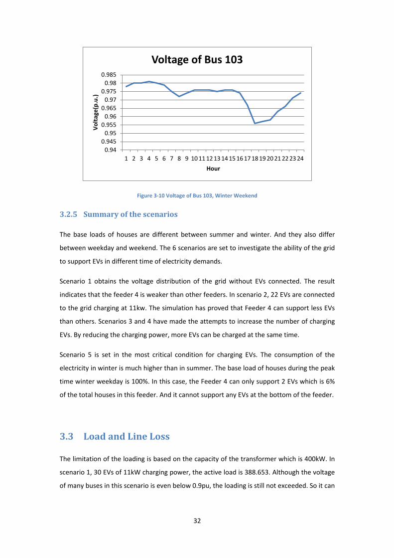
Scenario 6: Winter Weekend, 11kW, whole day

At most of the time, the load demand on a winter weekend is lower than a winter weekday.

So the number of EVs can be supported is expected to be the same or a little more. In this

scenario, Bus 103 is chosen to observe the voltage variation in a whole day. The number of

EVs connected to the grid is 21 (2 EVs in Feeder 4) as in Scenario 5. The voltage drops to

0.956 during the time 17:00 to 18:00. From the curve it can be seen that the off peak time

has less pressure of voltage drop. Therefore, the charging time is more suitable to be

arranged to the time from 22:00 to 07:00.

27%

50%

100%

6%

100%

0%

20%

40%

60%

80%

100%

120%


Possible number of EVs(%), 11kW

32

Figure 3-10 Voltage of Bus 103, Winter Weekend

3.2.5 Summary of the scenarios

The base loads of houses are different between summer and winter. And they also differ

between weekday and weekend. The 6 scenarios are set to investigate the ability of the grid

to support EVs in different time of electricity demands.

Scenario 1 obtains the voltage distribution of the grid without EVs connected. The result

indicates that the feeder 4 is weaker than other feeders. In scenario 2, 22 EVs are connected

to the grid charging at 11kw. The simulation has proved that Feeder 4 can support less EVs

than others. Scenarios 3 and 4 have made the attempts to increase the number of charging

EVs. By reducing the charging power, more EVs can be charged at the same time.

Scenario 5 is set in the most critical condition for charging EVs. The consumption of the

electricity in winter is much higher than in summer. The base load of houses during the peak

time winter weekday is 100%. In this case, the Feeder 4 can only support 2 EVs which is 6%

of the total houses in this feeder. And it cannot support any EVs at the bottom of the feeder.

3.3 Load and Line Loss

The limitation of the loading is based on the capacity of the transformer which is 400kW. In

scenario 1, 30 EVs of 11kW charging power, the active load is 388.653. Although the voltage

of many buses in this scenario is even below 0.9pu, the loading is still not exceeded. So it can

0.94 0.945

0.95 0.955

0.96 0.965

0.97 0.975

0.98 0.985

1 2 3 4 5 6 7 8 9 10 11 12 13 14 15 16 17 18 19 20 21 22 23 24

Volta

ge(p

.u.)

Hour

Voltage of Bus 103

33

be concluded that the loading is not the main limitation of the grid. The overall load and line

loss is shown in Table 3-6.

Table 3-6 Load of the transformer and Loss of the Grid

Load (kW)

Load (kvar)

Line Loss (kW)

Line Loss (kvar)

S1 Summer Weekday 47.653 12.119 0.452 0.324 S2 Summer Weekday 30EVs 11kw 388.653 12.119 28.583 22.385 S2 Summer Weekday 22EVs 11kw 300.653 12.119 11.749 12.093 S3 Summer Weekday 42EVs 5kw 257.653 12.119 9.503 9.064 S5 Winter Weekday 35EVs 5kw 283.08 27.487 11.066 11.232 S6 Winter Weekday 22EVs 11kw 350.08 27.487 15.356 17.16

Figure 3-11 Comparison of Load and Loss

Figure 3-11 is the comparison of the load and loss in different scenarios. All these 4 scenarios

meet the voltage requirement. It can be observed that the line loss is a small part compared

to the total load. And the loss does not differ much between different scenarios with

different load.

Based on the analyses above, rather than the load and loss of the grid, the voltage will be

the main characteristic to analyze.

0

50

100

150

200

250

300

350

400

S2 Summer Weekday 22EVs

11kw

S3 Summer Weekday 42EVs

5kw

S5 Winter Weekday 35EVs

5kw

S6 Winter Weekday 22EVs

11kw

Pow

er (k

W)

Scenarios

Line Loss (kW)

Load (kW)

34

Three critical lines are selected to be compared. They are the first line of Feeder 1, Feeder 2

and Feeder4. The loading of these three lines are presented in Figure 3-12. The L22 has the

most critical loading stress of the three. This is because that Feeder 2 supports 11 EVs which

is 50% of total in this condition.

Figure 3-12 Loading of the lines, winter weekday, peak time

3.4 Feeder Reformation to Improve the Behaviour of the

Grid

In the section 3.2, 7 scenarios have been analyzed to observe the behaviours of the network

with integration of EVs. It can be seen that Feeder 2 is stronger than other feeders for

supporting EVs, while Feeder 4 is weaker. The possible reason for Feeder 4 to be weak is

that it has too many levels of branch feeders, so the impedance of this feeder is much bigger

than other feeders.

The thought is to divide the Feeder 4 into two new independent feeders. It may improve the

ability of supporting EVs. As shown in Figure 3-13, the blue line is created to connect Bus 81

directly to the main Bus 2. In that way, two new feeders, called Feeder 4_1 and Feeder 4_2,

are established from original Feeder 4. The parameters of the new blue line are shown in

Table 3-7. The length of the line is calculated by summing four lines nearby (0.217km,

0.072km, 0.073km, 0.079km).

69.83

141.28

65.73

0

20

40

60

80

100

120

140

160

L1 L22 L55

Load

ing(

kw)

Name of the lines

Loading of the lines (kW)

35

Figure 3-13 Divide Feeder 4 into two new feeders

Table 3-7 Parameters of the new blue line

Length(

km)

Resistance

R'(Ohm/km)

Reactance

X'(Ohm/km)

Resistance

R'(pu)

Reactance

X'(pu)

0.441 0.2075 0.07225663 0.132079699 0.045993417

In Scenario 5, peak time on winter weekday, the network can only support 2 EVs at front

part of Feeder 4. In this new network, 12 EVs is put into the grid at the same position. Figure

3-14 reveals the distinct improvement after the division of Feeder 4. It can be said that new

Feeder 4_1 and 4_2 could support more than 12 EVs at the same condition (peak time on

winter weekday). The reformation is done by setting a new line.

36

Figure 3-14 Comparison of new grid and original grid

3.5 Conclusion

In this chapter, the operation of the distribution network has been analyzed. 6 scenarios are

set due to the different load demands between winter and summer, weekday and weekend.

The objective is to observe the ability of the grid to support connected EVs.

It can be concluded that in summer the grid can support more EVs than in winter, for the

houses have more consumption in the winter. There are more needs for heating and lighting

in the winter. Furthermore, there is more consumption during the weekdays than the

weekends.

There are evidences to prove that Feeder 4 is weaker than the other feeders. It is a long

feeder and the voltage easily drops at the end of the feeder. A solution to improve the

behaviour of Feeder 4 is given. By splitting the Feeder 4 into two new feeders, the ability of

supporting EVs is markedly improved.

The loading and loss of the grid are analyzed. They are not the main limitations of supporting

EVs. The voltage is proved to be the main bottleneck of the distribution grid.

0.925

0.93

0.935

0.94

0.945

0.95

0.955

0.96

0.965

0.97

57

59

61

63

65

67

69

71

73

75

77

79

81

83

85

87

89

91

93

95

97

99

101

103

Volta

ge(p

.u.)

Bus Number

Voltage of new Feeder 4_1 and 4_1 (12EVs) Voltage of original Feeder 4 (2EVs)

37

4 Stochastic Process of EV Integration

4.1 Introduction

In Chapter 3, the distribution grid has been tested with different scenarios. The charging

time is chosen to be peak time. During this time, the load demands have extreme value that

can be analyzed. The maximum charging power is 11kW, which has been used in some cases

to see the ability of the grid to support EVs. Some charging power has been assumed, like

5kW and 2kW, to allow more EVs to charge at the same time. In [14] [15], some work of

optimization has been done based on assumption of initial state.

In real life, the behaviours of EV owners could be complex. For instance, the driving distance

of each EV differs from others; the time of leaving/arriving home is not the same; some

families may have needs to drive a lot during weekends etc. Those are random behaviours

which also can be predicted based on certain patterns. The patterns can be obtained by

large number of survey.

Using those patterns, a stochastic process can be done to generate random data of EVs. This

data can reflect the behaviours of EVs in real life. A model can be built on this stochastic

process which could make the analyses of the network more realistic. Furthermore, a dumb

charging plan based on the stochastic data could be made.

4.2 The Driving Pattern and the Available Charging Times

4.2.1 The Driving Pattern

The main charging places here are the houses of EV owners. The EVs are not considered to

be charged at working parking lot or other charging station in this project. So the driving

pattern mainly refers to the driving distance. The available charging times are the times

during which the EVs are parking at home. Hence the times of EVs leaving/arriving home are

essential to the case.

38

The cases studied in this project are based on Danish power system. Therefore the driving

pattern has to be the transportation data of Denmark. There are based on three data bases

[38]:

AKTA data (GPS-based data that follow the vehicles);

MDCars (Database of Odometer readings);

TU data (Danish National Transport Survey).

AKTA data are based on the data recorded by GPS with certain participated drivers. Hence,

the accuracy of this data is quite high. However, there are only 360 cars in this data base,

and the owners all live in Copenhagen [38]. So the samples can hardly represent the

behaviours of the majority of car owners in Denmark. The MDCars data are from the

collection of odometer data in cars. It has two years data for private cars [38].

TU data provided by Technical University of Denmark is a Danish National Travel Survey data.

It was first conducted in 1975, and about 270,000 Danish car owners participated in the

survey since 1992 [39]. The data contain 750,000 trip information with details [39]. The

group of drivers, region, age, income and day of week are all collected in the survey.

Through this data, a proper picture of driving pattern can be revealed. So this data base is

used in this project to do the stochastic process.

The Figure 4-1 shows the distribution on transport means in Denmark in 2012. From both

distance and times of trips sides, the travels by vehicles occupy the most part. Even though

Denmark is well known with promoting bicycles, the vehicles are still the main transport

means. Many families go to work by cars and the number of cars is growing. EVs analyzed in

this project are seen having the similar behaviours as normal gasoline cars.

39

Figure 4-1 Distribution of transport means [40]

Table 4-1 presents the average driving distance in Denmark based on TU data. From this

table it can be observed that the average driving distance of all days is less than 30km. This

may differ from other countries like America. Since America has larger territory and drivers

are expected to drive more distance. Relatively short driving distance is a suitable factor to

promote EVs in Denamrk. Because the technique of EV batteries has limited the driving

distance of EVs.

The other characteristic shown in Table 4-1 is that EVs tend to drive less on weekends and

holidays. The reduction of driving distance at those times could be explained by reduction of

work related travels.

Table 4-1 Average driving distance in Denmark [38]

Average

Distance(km)

All Days 29.48

Monday 28.39

Tuesday 31.57

Wednesday 32.19

Thursday 30.98

Friday 33.96

Saturday 26.48

Sunday 24.4

Holiday 18.9

40

The distributions of driving distance on weekdays, weekends and holiday are shown in

Appendix C. Based on these data, the distributions of distance are plotted in Figure 4-2 and

Figure 4-3.

Figure 4-2 Distribution of driving distance on weekdays

Figure 4-3 Distribution of driving distance on weekends and holiday

0 0.05

0.1 0.15

0.2 0.25

0.3 0.35

0.4 0.45

0.5

0 20 40 60 80 100 200 300 400 500 700 900

Percentage

Driving Distance(km)

Distribution of distance on weekdays

Mon

Tue

Wed

Thu

Fri

0

0.1

0.2

0.3

0.4

0.5

0.6

0.7

Percentage


Distribution of distance on weekends and holiday

Sat

Sun

Holiday

41

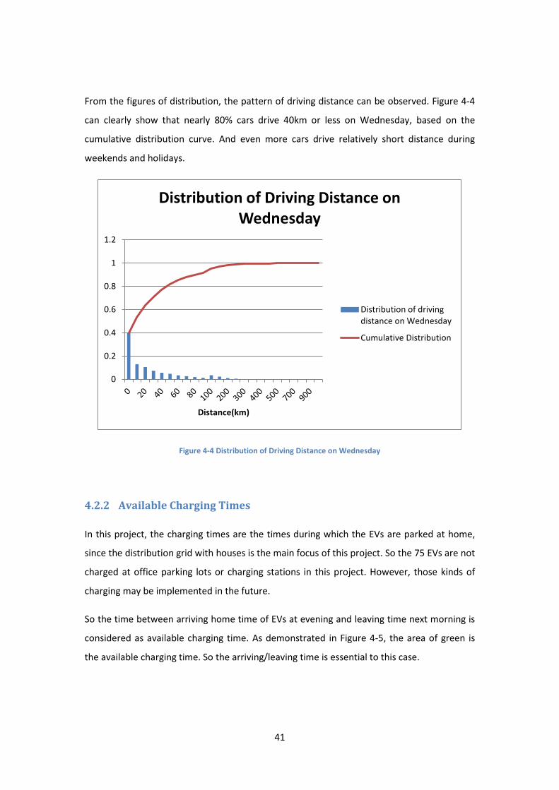
From the figures of distribution, the pattern of driving distance can be observed. Figure 4-4

can clearly show that nearly 80% cars drive 40km or less on Wednesday, based on the

cumulative distribution curve. And even more cars drive relatively short distance during

weekends and holidays.

Figure 4-4 Distribution of Driving Distance on Wednesday

4.2.2 Available Charging Times

In this project, the charging times are the times during which the EVs are parked at home,

since the distribution grid with houses is the main focus of this project. So the 75 EVs are not

charged at office parking lots or charging stations in this project. However, those kinds of

charging may be implemented in the future.

So the time between arriving home time of EVs at evening and leaving time next morning is

considered as available charging time. As demonstrated in Figure 4-5, the area of green is

the available charging time. So the arriving/leaving time is essential to this case.

0

0.2

0.4

0.6

0.8

1

1.2

Distance(km)

Distribution of Driving Distance on Wednesday

Distribution of driving distance on Wednesday

Cumulative Distribution

42

Figure 4-5 Available Charging Time

Normally, the arriving/leaving time of cars is similar in many countries, since most people

work at day and get home by evening. The arriving time data in this project is from National

Household Travel Survey (NHTS). The data are based on the survey of American vehicle users.

Because of the similarity, it could be used in case of Denmark. The arriving data are plotted

in Figure 4-6. It can be seen that many cars arrive home around 18:00.

Figure 4-6 Arriving time [41]

0.00%

10.00%

20.00%

30.00%

40.00%

50.00%

60.00%

70.00%

80.00%

90.00%

100.00%

0.00%

2.00%

4.00%

6.00%

8.00%

10.00%

12.00%

14.00%

00:0

0-01

:00

01:0

0-02

:00

02:0

0-03

:00

03:0

0-04

:00

04:0

0-05

:00

05:0

0-06

:00

06:0

0-07

:00

07:0

0-08

:00

08:0

0-09

:00

09:0

0-10

:00

10:0

0-11

:00

11:0

0-12

:00

12:0

0-13

:00

13:0

0-14

:00

14:0

0-15

:00

15:0

0-16

:00

16:0

0-17

:00

17:0

0-18

:00

18:0

0-19

:00

19:0

0-20

:00

20:0

0-21

:00

21:0

0-22

:00

22:0

0-23

:00

23:0

0-24

:00

Share of Sampled Vehicles Cumulative Frequency

43

In order to get the leaving time of EVs, the similar distribution shape is assumed. Move the

ridge of wave of arriving time from 17:00-18:00 to 06:00-07:00 to present the peak of

leaving time distribution. The departure time distribution is formed in Figure 4-7.

Figure 4-7 Distribution of Departure/Arrival Time

4.3 The Consumption Needed for EVs in the Grid

Electric vehicles normally are more efficient than petrol cars. The average consumption is

0.15-0.25kWh/km including the charging losses, while the petrol cars have to use equivalent

at least 0.5 kWh to drive one kilometre [42]. Table 4-2 shows an example of consumption of

4 types of EVs. The FEV refers to Full Electric Vehicles, and the PHEV refers to Plug-in Hybrid

Electric Vehicles.

Table 4-2 Example of consumption of EVs [42]

Electricity consumption

kWh/km

Trip on electricity

km/year

Annual consumption

MWh/year

FEV 0.25 0.25 17400 4.34

FEV 0.17 0.17 17500 2.97

PHEV 0.25 0.25 14100 3.53

PHEV 0.17 0.17 14000 2.38

0.00%

2.00%

4.00%

6.00%

8.00%

10.00%

12.00%

14.00%

Arrival

Departure

44

In this project, the EVs are assumed to use 0.15kWh for one kilometre. Since the high

efficiency is the tendency in the future. Thus the energy needed per day could be calculated

by following formula:

0.15 /E kWh km D= × (E4-1)

where D is the distance(km) has been driven per day.

4.4 The Dumb Charging

Dumb charging is a charging method that allows EV owners to charge their EVs whenever

they need. Normally the charging starts at the time they get home. When the EVs are

plugged into the mains, the charging begins. And the charging power intends to be the

maximum. In this case, the charging power could be 11kW. So the dumb charging is not

controlled and planed. It could cause fluctuation in the distribution grid.

The dumb charging has some characteristics [43]:

1. Vehicles begin to charge as soon as plugged in. And normally keep being charged

until full charge of the batteries;

2. The load variability in the distribution grid will increase because of the dumb

charging;

3. The dumb charging normally does not participate in balancing the power system or

V2G.

Many EVs nowadays use dumb charging, because it is convenient and fast. People are used

to charge EVs till the batteries are full, like any other electric equipment. Dumb charging is

important to network case study. The simulation of dumb charging could affect the ability

and stability of the distribution grid to support EVs. A strong network should meet the

requirements of dumb charging and minimize the jeopardizing caused by dumb charging.

A dumb charging plan will be made in this chapter based on the stochastic data.

45

4.5 The Stochastic Simulation

4.5.1 The Stochastic Process for Driving Distance and Available Charging

Time

The main goal of this section is to use the driving patterns to obtain the stochastic data of

energy demands and available charging times of the EVs. The energy demand is based on

the driving distance. And the available charging time is between the arriving time and

leaving time.

Normally the cars drive more distance during weekday. The consumption of electricity is also

higher during weekdays than weekends. So in order to fulfil the daily driving requirements, a

weekday like Wednesday is selected to be analyzed.

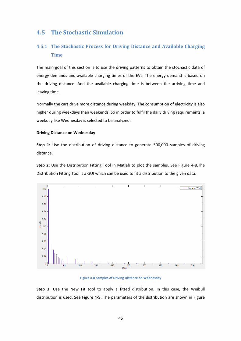
Driving Distance on Wednesday

Step 1: Use the distribution of driving distance to generate 500,000 samples of driving

distance.

Step 2: Use the Distribution Fitting Tool in Matlab to plot the samples. See Figure 4-8.The

Distribution Fitting Tool is a GUI which can be used to fit a distribution to the given data.

Figure 4-8 Samples of Driving Distance on Wednesday

Step 3: Use the New Fit tool to apply a fitted distribution. In this case, the Weibull

distribution is used. See Figure 4-9. The parameters of the distribution are shown in Figure

46

4-10. For Weibull distribution, a=33.4061 and b=0.798717 are important parameters for next

step.

Figure 4-9 A fitted distribution

Figure 4-10 Parameters of new fitted distribution

Step 4: Using appropriate source code in Matlab to generated random data of driving

distance for 75 EVs, with the parameters of new fitted distribution. Part of the code is shown

in Appendix H. Figure 4-11 is the stochastic data of driving distance generated by the

program. It can be seen that most EVs drive less than 50 km per day.

47

Figure 4-11 Stochastic Data of Driving Distance

Step 5: Using the formula of energy consumption in 4.3. The energy needed for each EV is

calculated with driving distance. See Figure 4-12. It can be observed that many EVs need less

than 10 kWh per day to fulfil the driving demand.

Figure 4-12 The energy needed for each EV

0 50 100 150 200 250 300 350 400 1 6

11 16 21 26 31 36 41 46 51 56 61 66 71


The

No.

of E

Vs

Stochastic Data of Driving Distance(km) for 75 EVs

0

10

20

30

40

50

60

1 4 7 10 13 16 19 22 25 28 31 34 37 40 43 46 49 52 55 58 61 64 67 70 73

Ener

gy(k

Wh)

The No. of Evs

Energy

48

Available Charging Time

Step 1: Use the distribution of arriving time to generate 8,601 samples of arriving time. The

number 8,601 is selected because the cumulative frequency of the given data of arriving

time is 86.01%.

Step 2: Use the Distribution Fitting Tool in Matlab to plot the samples of arriving time. See

Figure 4-13. Many EVs arrive home from the afternoon till the evening.

Figure 4-13 Samples of arriving time

Step 3: Find a new fitted distribution. For these samples of arriving time, the Normal

distribution is used. See Figure 4-14. The parameters mu=16.8461, sigma=3.60194.

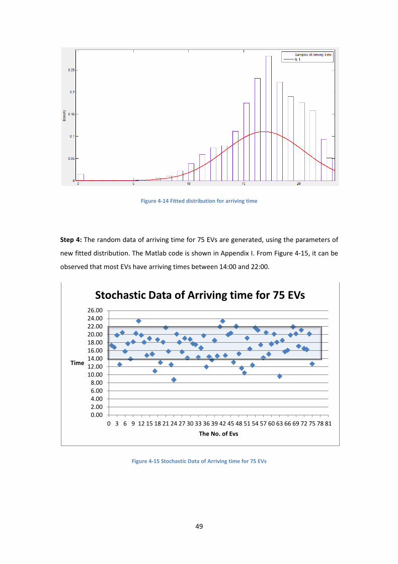
49

Figure 4-14 Fitted distribution for arriving time

Step 4: The random data of arriving time for 75 EVs are generated, using the parameters of

new fitted distribution. The Matlab code is shown in Appendix I. From Figure 4-15, it can be

observed that most EVs have arriving times between 14:00 and 22:00.

Figure 4-15 Stochastic Data of Arriving time for 75 EVs

0.00 2.00 4.00 6.00 8.00

10.00 12.00 14.00 16.00 18.00 20.00 22.00 24.00 26.00

0 3 6 9 12 15 18 21 24 27 30 33 36 39 42 45 48 51 54 57 60 63 66 69 72 75 78 81

Time

The No. of Evs

Stochastic Data of Arriving time for 75 EVs

50

Step 5: Use similar method to obtain the stochastic data of departure time for 75 EVs in

Figure 4-16. Most of the EVs leave home between 4:00 and 12:00.

Figure 4-16 Stochastic data of departure time for 75 EVs

4.5.2 Charging plan using stochastic data on Wednesday in summer

In section 4.5.1, the random data of the energy needed for each EV on Wednesday is

obtained. Based on these data a charging plan is made. The flow diagram of charging plan

for each EV is given in Figure 4-17.

0.00 2.00 4.00 6.00 8.00

10.00 12.00 14.00 16.00 18.00 20.00 22.00 24.00 26.00

0 3 6 9 12 15 18 21 24 27 30 33 36 39 42 45 48 51 54 57 60 63 66 69 72 75 78 81

Time

The No. of EVs

Stochastic data of departure time for 75 EVs

51

Figure 4-17 Charging Flow Diagram for Each EV

For almost all the EVs, the available charging time during the night is adequate. Hence the

arriving time is the major factor of available charging time. The random arriving time is also

obtained from the section 4.5.1.

52

Based on the charging plan for each EV, a Matlab program is made to do the load flow

calculation for each hour in the distribution grid. First, the matrices of energy needed and

arriving time is set. Then check from hour 1(00:00 to 01:00) to hour 24(23:00 to 24:00). Each

EV corresponds to a unique hour of arriving. When the EV arrives, it starts to charge. If the

energy needed of this particular car is less or equal to 11kWh, for instance 5kWh, it charges

at 5kW. Or if the energy needed is more than 11kWh, for instance 30kWh, it charges at

11kW and charges remain at following hours. When the energy consumption for driving is

recharged, it stops charging. So a matrix with the time and charging power of all EVs can be

obtained. A part of the matrix is shown in Table 4-3. The full table is in Appendix D. Each

column has the total consumption of EVs in one hour.

In the table, most EVs charge from noon 12:00 till night 24:00. They begin to charge as soon

as they arrive home. There are more EVs charging at the peak times (16:00-20:00) than

other times.

Table 4-3 A part of matrix of charging plan

16:00-

17:00

17:00-

18:00

18:00-

19:00

19:00-

20:00

20:00-

21:00

21:00-

22:00

22:00-

23:00

23:00-

24:00

0.64 0 0 0 0 0 0 0 EV1

0.03 0 0 0 0 0 0 0 EV2

0 0 0 1.18 0 0 0 0 EV3

0 0 0 0 0 0 0 0 EV4

0 0 0 2.3 0 0 0 0 EV5

2.66 0 0 0 0 0 0 0 EV6

0 0.27 0 0 0 0 0 0 EV7

0 0 0 0 0 0 0 0 EV8

0 0.67 0 0 0 0 0 0 EV9

0 0 0 7.26 0 0 0 0 EV10

0 0 0 0 0 0 2.21 0 EV11

0 0 0 11 11 4.6 0 0 EV12

0 4.12 0 0 0 0 0 0 EV13

Combining each the charging power in each column with corresponding house load, the

power consumed in each bus is obtained. Afterwards, then load flow is calculated. As shown

53

in Figure 4-18, the quality of voltage meets the requirement (≥0.94 pu). One of most

constrained buses, Bus 103 is chosen in Figure 4-19. It can be seen that there is a steep drop

during 19:00-20:00. This phenomenon is caused by six EVs charging at this time in the

Feeder 4, which significantly increases the loading.

Figure 4-18 Bus voltage at hour 18, Wednesday, summer

0.91

0.92

0.93

0.94

0.95

0.96

0.97

0.98

0.99

1

1.01

1 5 9 13

17

21

25

29

33

37

41

45

49

53

57

61

65

69

73

77

81

85

89

93

97

101

105

Volta

ge(p

.u.)

Bus Number

Voltage, 17:00-18:00, Wednesday, Summer

54

Figure 4-19 Voltage (pu), Bus 103, Wednesday, Summer

4.5.3 Charging plan using stochastic data on Wednesday in winter

From the section 4.5.2, it has been proved that the grid can support the charging of EVs with

stochastic pattern in a summer weekday. A Wednesday in winter is picked to be analyzed to

compare the results with the section 4.5.2.

The energy needed of EVs is assumed to be the same as in summer. The consumption of

house is more, as shown in Appendix B. The voltage comparison is shown in Figure 4-20 and

Figure 4-21.

0.92

0.93

0.94

0.95

0.96

0.97

0.98

0.99

1

00:0

0-01

:00

01:0

0-02

:00

02:0

0-03

:00

03:0

0-04

:00

04:0

0-05

:00

05:0

0-06

:00

06:0

0-07

:00

07:0

0-08

:00

08:0

0-09

:00

09:0

0-10

:00

10:0

0-11

:00

11:0

0-12

:00

12:0

0-13

:00

13:0

0-14

:00

14:0

0-15

:00

15:0

0-16

:00

16:0

0-17

:00

17:0

0-18

:00

18:0

0-19

:00

19:0

0-20

:00

20:0

0-21

:00

21:0

0-22

:00

22:0

0-23

:00

23:0

0-24

:00

Volta

ge(p

u)

Time

Voltage(p.u.), Bus 103, Wednesday, Summer

55

Figure 4-20 Comparison of voltage, 17:00-18:00

Figure 4-21 Comparison of voltage, Bus 103

Arriving home at different time has reduced the congestions in the distribution grid.

Normally the grid allows EVs to charge as soon as they arrive home. However, for the

economic reason, charging as soon as arriving is not always recommendable. At midnight,

0.9

0.92

0.94

0.96

0.98

1

1.02

1 5 9 13

17

21

25

29

33

37

41

45

49

53

57

61

65

69

73

77

81

85

89

93

97

101

105

Volta

ge(p

u)

Bus No.

Comparison of voltage(p.u.), 17:00-18:00

WinterWed SummerWed

0.91 0.92 0.93 0.94 0.95 0.96 0.97 0.98 0.99

1

00:0

0-01

:00

01:0

0-02

:00

02:0

0-03

:00

03:0

0-04

:00

04:0

0-05

:00

05:0

0-06

:00

06:0

0-07

:00

07:0

0-08

:00

08:0

0-09

:00

09:0

0-10

:00

10:0

0-11

:00

11:0

0-12

:00

12:0

0-13

:00

13:0

0-14

:00

14:0

0-15

:00

15:0

0-16

:00

16:0

0-17

:00

17:0

0-18

:00

18:0

0-19

:00

19:0

0-20

:00

20:0

0-21

:00

21:0

0-22

:00

22:0

0-23

:00

23:0

0-24

:00

Volta

ge(p

u)

Time

Comparison of voltage, Bus 103

WinterWed SummerWed

56

when the house consumption is relatively low and the wind production is high, the price of

electricity would drop. Charging at those times could benefit both grid and owners of EVs.

During the peak time in the winter weekday, the Feeder 4 cannot support all the EVs to

charge as they arriving home. Using this dumb charging plan may cause steep voltage drop

at the bottom of the feeder. A few EVs need to be moved to other times for charging.

4.6 Conclusion

In this chapter, the stochastic data of the behaviours of EVs are generated using the Monte

Carlo Method. With arriving time and leaving time, the available charging times for EVs are

obtained. The energy demands for each EV are calculated based on the random driving

distance.

A charging plan is then made based on the stochastic data. It is a dump charging plan with

which EVs start to charge as soon as they arrive. The voltage drops distinctly during the peak

time because of the arrivals of many EVs and the peak demands of houses. The grid has

much stress during these times. The cost of charging at these times is also high because of

the large amount consumption of electricity.

57

5 Optimization of Charging Plans

5.1 Introduction

In Chapter 3, 6 scenarios have been set to analyze the operation behaviours of the

distribution grid. The number and charging power of the EVs have been assumed to meet

the operation requirements of the grid. The places to put connected EVs in the grid are also

manually selected. These assumptions make it easy to observe the operation features of the

grid. However, it is not realistic because the behaviours of EV owners are not deterministic.

Based on the stochastic analysis in the previous chapter, simulations were conducted to

reflect a situation closed to the real behaviours of the EVs in the grid. The EVs drive different

distance a day and arrive home at different time. The simulation is based on certain pattern

supported by surveys. With the stochastic data, charging plans have been made. EVs start to

charge when they arrive home. Since most EVs arrive between 14:00 and 22:00 as shown in

Figure 4-15, and 16:00 to 20:00 are normally the peak time of electricity consumption, it

may cause huge stress on the grid operation.

An optimization methodology is applied in this Chapter, focusing on dispersing the

congestions of the grid by moving the charging time of the EVs to off-peak times of the

consumption of electricity. The off-peak times of electricity are normally midnight when the

price of electricity is relatively low. So by optimizing the charging plans, the economic

benefit for aggregators and EV owners may be achieved.

There are some optimized charging plans proposed in [15] [44] and [45]. Most of the plans

are based on assumptions rather than stochastic data. In this project, the stochastic process

is used to make the optimization outcomes more realistic.

5.2 The Smart Charging

Smart charging is a charging method that requires systematic control system. The efficient

management is crucial in this method. Instead of charging immediately and automatically

when the EVs being plugged in, the charging happens in different time period at different

charging power controlled by the system. This requires the coordination and communication

58

between TSO, DSO, aggregators, EVs owners etc. The data of electricity price should be

updated day ahead or even hour ahead. After the smart charging, the SOC of the batteries

should meet the demand of driving distance needed. The Smart Grid proposed in Denmark

aims to provide a suitable environment for smart charging. Figure 5-1 shows an example of

smart charging system.

Figure 5-1 An example of smart charging system [44]

The smart charging has following features [43]:

1. Charging plan is normally made one day ahead;

2. The plan can be changed intra-day.

3. The spinning and tertiary reserves can be provided by EVs, along with V2G.

With planed charging at different time period with different charging power, the pressure of

operation of the distribution grid can be reduced. This is a hierarchical structure of

controlling. The EV owners have to commit to the agreement of controlling. Besides the fact

that smart charging can help stabilize the bus voltage and prevent the congestion of the grid,

the benefit could be made by smart charging is also attractive to EV owners to make such

agreement. Figure 5-2 shows the system and the market benefit of smart charging EVs. The

market price of smart EVs is also cheaper than the dumb EVs.

59

Figure 5-2 Example of benefits from smart charging EVs [43]

In Denmark, the high penetration of wind power could lead the electricity price to very low

during windy days. The smart charging makes it possible for EVs owners to benefit from the

electricity price fluctuation.

5.3 Wind Power Case in the Optimization Process

The penetration of the wind is very high in Danish power system. The production of wind

power could seriously affect the supply and demand relationship of the electricity, thereby

affect the price of the electricity. The table of the Elspot price and corresponding wind

production for 8 typical days is shown in Appendix E.

60

Figure 5-3 Wind Production of two winter weekdays

Figure 5-4 Elspot Price of two winter weekdays

Figure 5-3 and Figure 5-4 show the relationship between the wind production and the price

of the electricity in two typical winter weekdays. The price in the windy day goes very low, at

some hours even closed to zero. This probably caused by that the wind production exceeds

the demand of the electricity. In the day with low wind speed, the price goes extremely high,

even over 1000 DKK/MWh at some hours. It is because that there is little wind production

and most of the electricity has to be generated by conventional power plant.

Beside the wind production, the price could also be affected by the demand of consumption,

operations of power system of neighbour countries, market fluctuation etc. In this project,

0

500

1000

1500

2000

2500

3000

13 14 15 16 17 18 19 20 21 22 23 24 1 2 3 4 5 6 7 8 9 10 11 12

Win

d Pr

oduc

tion

(MW

h/h)

Hour Winter Windy Weekday Winter Weekday with Low Wind Speed

0

200

400

600

800

1000

1200

1400

1600

1800

13 14 15 16 17 18 19 20 21 22 23 24 1 2 3 4 5 6 7 8 9 10 11 12

Pric

e (D

DK/M

Wh)

Hour Winter Windy Weekday Winter Weekday with Low Wind Speed

61

some typical days are chosen mainly based on the wind condition. The price of electricity of

typical days is shown in Figure 5-5, Figure 5-6 and Figure 5-7.

Figure 5-5 Elspot Price of electricity at two winter weekends

Figure 5-6 Elspot Price of electricity at two summer weekdays

Figure 5-7 Elspot Price of electricity at two summer weekends

0

200

400

600

800

1000

13 14 15 16 17 18 19 20 21 22 23 24 1 2 3 4 5 6 7 8 9 10 11 12

Pric

e (D

DK/M

Wh)

Hour Winter Windy Weekend

Winter Weekend with Low Wind Speed

0

100

200

300

400

500

13 14 15 16 17 18 19 20 21 22 23 24 1 2 3 4 5 6 7 8 9 10 11 12

Pric

e (D

DK/M

Wh)

Hour Summer Windy Weekday

Summer Weekday with Low Wind Speed

0

100

200

300

400

13 14 15 16 17 18 19 20 21 22 23 24 1 2 3 4 5 6 7 8 9 10 11 12

Pric

e (D

DK/M

Wh)

Hour Summer Windy Weekend

Summer Weekend with Low Wind Speed

62

5.4 The Objective and Methodology of the Optimization

The main objective of the optimization is to minimize the cost in the EV charging plans, while

meeting the requirement of the stable operation of the distribution grid. The price data is

from [30] which is the Elspot price in DKK/MWh. To make it more practical, the price is

converted to DKK/KWh and added 2 DKK/KWh tax with it [34]. The adding tax will not affect

the amount of the reduction of charging cost. Since the available charging times are mostly

from afternoon till next day morning, it is wise to choose the 24 hour duration within 12:00

to next day 12:00. Table 5-1 shows an example of converted price in a winter windy day. The

complete table of price used in the optimization is in Appendix F.

Table 5-1 Price used in optimization, A winter windy day

Hour Elspot Price, DKK/MWh Price, with Tax, DKK/KWh

13 248.32 2.24832 14 248.62 2.24862 15 248.54 2.24854 16 250.7 2.25070 17 252.41 2.25241 18 251.22 2.25122 19 249.73 2.24973 20 245.72 2.24572 21 251 2.25100 22 214.8 2.21480 23 214.5 2.21450 24 118.92 2.11892 1 37.91 2.03791 2 0.52 2.00052 3 0.3 2.00030 4 0.67 2.00067 5 74.34 2.07434 6 81.78 2.08178 7 154.11 2.15411 8 294.99 2.29499 9 244.96 2.24496

10 244.44 2.24444 11 246.67 2.24667 12 247.26 2.24726

The procedure of the optimization for smart charging is explained as following:

1. Generate the stochastic data of energy need and arriving time of EVs.

63

2. Search the hour with lowest price of electricity.

3. Charge the arrived EVs at the hour of lowest price at 11kW. The remaining needed

energy will be moved to the hour of second lowest price. If the energy need is less

than 11kWh, for instance 6kWh, then charge at 6kW.

4. Run the load flow calculation, set the constraint of 0.94 pu≤Voltage≤1.06pu

5. If the voltage of any buses is lower than 0.94pu, move certain number of EVs from

the hour of lowest price to the hour of second low price. The number of moved EVs

is based on the analyses of base cases in Chapter 3. Run the load flow again and

repeat this step until the hour of lowest price in which the voltage meets the

constraint.

6. Repeat the same step 3, 4, 5 to the hour of second low price. Then move to the hour

of third low price etc. Until all the EVs are fully charged.

The optimization process is done by using “fmincon” function in Matlab. The objective

function is

10 75

1 1( )m nm

m nCt c p

= =

= ×∑ ∑ (E5-1)

Where Ct is the total cost of charging, m is the hour, n is the number of EVs, c is the price of

a particular hour, p is the charging power at that hour of an EV which is variable.

The optimization function subjects to:

1. 0.94 . .nV p u≥ , nV is the voltage of every cable box.

2. 10

1n nm

mE p

=

=∑ , nE is the energy need of EV n. This ensures that all the EVs are fully

charged.

3. 11nmp kW≤ , the maximum charging power of each EV is 11kW.

The flow diagram of the optimization is shown in Figure 5-8.

64

Figure 5-8 Flow diagram of optimization

65

5.5 The Simulation

5.5.1 Scenario 1: Winter Windy Weekday

Based on the stochastic data of arriving time and leaving time generated in Section 4.5.1,

most of the EVs are available between 19:00 and 05:00. These 10 hours are chosen to

simplify the optimization and reduce the processing time period. The price of these 10 hours

in a winter windy weekday is shown in Table 5-2.

Table 5-2 Price of electricity in a winter windy weekday

Hour 20 21 22 23 24 1 2 3 4 5 Price(DKK/kWh)

2.24572

2.25100

2.21480

2.21450

2.11892

2.03791

2.00052

2.00030

2.00067

2.07434

The energy demand is also generated in Section 4.5.1. The outcome of the optimized

charging plans is in Figure 5-9. It can be observed in the plan that many EVs charge during

02:00-03:00 when the price is the lowest. If cannot be fully charged, these EVs charge at

01:00-02:00 and 03:00-04:00.

In the Feeder 4, however, only a few EVs can simultaneously charge during 02:00-03:00,

because of the constraint of voltage drop. The EVs are been placed on different time period

to charge in the order of price of electricity. The EV68 which needs 54.9 kWh takes 5 hours

to be fully charged. And because it is at the bottom part of the Feeder 4, it has not been

arranged to 01:00-04:00 to charge.

66

Figure 5-9 Optimized charging plan of a winter windy day

67

5.5.2 Scenario 2: Summer Weekday with Low Wind Speed

The same driving pattern as 5.4.1 has been chosen in this scenario. The time period is also

the same 10 hours. The price of electricity in a summer weekday with low wind speed is

shown in Table 5-3. The outcome of the optimization is presented in Figure 5-10.

Table 5-3 Price of electricity in a summer weekday with low wind speed

Hour 20 21 22 23 24 1 2 3 4 5 Price(DKK/kWh)

2.39420

2.35681

2.34543

2.36402

2.31286

2.17339

2.16707

2.16328

2.16083

2.16090

In this charging plan, the prices during 03:00-04:00 and 04:00-05:00 are very close. This

leads to that many EVs approximately evenly charge during these two hours. This disperses

the stress of the grid and enables more EVs to charge at low price periods.

68

Figure 5-10 Optimized charging plan of a summer day with low wind speed

69

Figure 5-11 shows the voltage of Bus 103 which is one of the most constrained buses in two

scenarios. Because of the charging of EVs, the voltage drops during the off-peak time 24:00

to 05:00. The constraint of the optimization function ensures that the voltage is above

0.94pu.

Figure 5-11 The voltage of Bus 103

5.6 Analyses of the Optimised Charging Plans

5.6.1 Voltage, Loading and Loss

In the scenario of winter windy weekday, many EVs charge during 24:00-04:00 since it is the

time when the price is low that day. The grid probably goes through with enormous stress

on operation during this time. The voltage, loading and loss of the grid at that time are

analyzed.

Figure 5-12 and Figure 5-13 show the voltage, load and loss of the grid during the four hours.

To make it clear to see the correspondence, there are colour marks on Time axis in Figure

5-13 corresponding to the voltage curve in Figure 5-12.

0.91

0.92

0.93

0.94

0.95

0.96

0.97

0.98

0.99

1

Volta

ge(p

.u.)

Time Voltage Bus 103 Winter Voltage Bus 103 Summer

70

Figure 5-12 Voltage during the four hours, winter windy weekday

Figure 5-13 Load and loss during the four hours, winter windy day

There are several things can be observed:

1. The highest loading happens during 02:00-03:00. This is because the price of

electricity is the lowest during this time, and the objective of this optimized charging

0.9

0.91

0.92

0.93

0.94

0.95

0.96

0.97

0.98

0.99

1

1.01

1 6 11

16

21

26

31

36

41

46

51

56

61

66

71

76

81

86

91

96

101

106

Volta

ge (p

.u.)

Bus No.

24:00-01:00

01:00-02:00

02:00-03:00

03:00-04:00

F1 F2 F3 F4 F5

0

50

100

150

200

250

24:00-01:00 01:00-02:00 02:00-03:00 03:00-04:00

Pow

er(k

W)

Time

Loss(kW)

Load(kW)

71

plan is to minimize the charging cost. It can be predict that more EVs charging at this

time, more benefit for EV owners will be made.

2. During these four hours, the highest loading is around 225 kW, which does not

exceed the capacity of the transformer. And there is relatively little loss during these

four hours.

3. The Feeder 2 only has distinct voltage drop during 02:00-03:00, when the price of

electricity is the lowest. That means that Feeder 2 has ability to charge most of EVs

in Feeder 2 at that time. Another word, Feeder 2 is a strong Feeder.

4. The bus voltage in Feeder 4 drops to the lowest during 24:00-01:00, when the price

of electricity is the highest in these four hours. While the load of charging EVs during

this hour does not differ from other 3 hours. However, due to the processing

sequence of the optimization program, the charging EVs in this hour are at the end

of the Feeder. Because Feeder 4 is a long and relatively weak Feeder, the steep

voltage drop of cable boxes at the last part of the Feeder could easily happen.

5. Feeder 1, 2, 3 and 5 all restore high voltage quality during 24:00-01:00. This can be

seen as a sign that most EVs connected to these Feeders are fully charged during

these four hours.

5.6.2 The optimized charging cost

The main objective of the optimization is to come out smart charging plans to reduce the

charging cost. In section 4.5.2, all EVs start to charge as soon as they arrive. The cost of this

kind of dumb charging is used to compare with the smart charging plans.

The data of dumb charging plan is in Appendix D. The price of electricity of a winter windy

weekday is chosen as Table 5-4. The total cost can be calculated by formula:

24 75

1 1( )DCW m nm

m nC c p

= =

= ×∑ ∑ (E5-2)

where CDCW is the total cost of the dumb charging plan. The outcome is CDCW = 996.55 DKK.

Table 5-4 Price of electricity of a winter windy weekday

Time Price(DKK/kWh) Time Price(DKK/kWh) 12:00-13:00 2.24832 24:00-01:00 2.03791 13:00-14:00 2.24862 01:00-02:00 2.00052 14:00-15:00 2.24854 02:00-03:00 2.0003 15:00-16:00 2.2507 03:00-04:00 2.00067

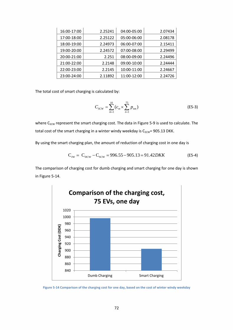
72

16:00-17:00 2.25241 04:00-05:00 2.07434 17:00-18:00 2.25122 05:00-06:00 2.08178 18:00-19:00 2.24973 06:00-07:00 2.15411 19:00-20:00 2.24572 07:00-08:00 2.29499 20:00-21:00 2.251 08:00-09:00 2.24496 21:00-22:00 2.2148 09:00-10:00 2.24444 22:00-23:00 2.2145 10:00-11:00 2.24667 23:00-24:00 2.11892 11:00-12:00 2.24726

The total cost of smart charging is calculated by:

10 75

1 1( )SCW m nm

m nC c p

= =

= ×∑ ∑ (E5-3)

where CSCW represent the smart charging cost. The data in Figure 5-9 is used to calculate. The

total cost of the smart charging in a winter windy weekday is CSCW= 905.13 DKK.

By using the smart charging plan, the amount of reduction of charging cost in one day is

rW DCW SCWC C C 996.55 905.13 91.42DKK= − = − = (E5-4)

The comparison of charging cost for dumb charging and smart charging for one day is shown

in Figure 5-14.

Figure 5-14 Comparison of the charging cost for one day, based on the cost of winter windy weekday

840

860

880

900

920

940

960

980

1000

1020

Dumb Charging Smart Charging

Char

ging

Cos

t (DD

K)

Comparison of the charging cost, 75 EVs, one day

73

Similarly, the cost of dumb charging in a summer weekday with low wind can be calculated,

CDCS=1065.52 DKK. The cost of smart charging in a summer weekday with low wind is

CSCS=971.68 DKK.

The average cost of dumb charging of two scenarios is:

(996.55 1065.52) / 2 1031.04DCAC DKK= + = (E5-5)

The average cost of smart charging of two scenarios is:

(905.13+971.68) / 2 938.41SCAC DKK= = (E5-6)

A calculation of the total reduction of smart charging for one year can be made based on

those average values:

365 365 376329.6 342519.65 33809.95r DCA SCAC C C DKK= × − × = − = (E5-7)

So for one year, using smart charging plans can reduce approximately 33809.95 DKK for 75

EV owners. See Figure 5-15.

Figure 5-15 Comparison of the charging cost for one year

It can be seen that by using smart charging plans, a considerable amount of charging cost

can be reduced. And in winter, summer, windy day or day with low wind speed, the smart

charging plan can always bring benefit to EV owners.

320000

330000

340000

350000

360000

370000

380000

Dumb Charging Smart Charging

Char

ging

Cos

t (DD

K)

Comparison of the charging cost, 75 EVs, one year

74

5.7 Conclusion

The price of electricity is affected by the demand of consumption and wind power

production etc. The optimal charging plans have been made to reduce the charging cost.

Available EVs charge at the period of low electricity price. Meanwhile, the stability and

reliability of the operation of the distribution grid are ensured. Two main scenarios are

chosen to compare the outcome in winter windy weekday and summer weekday with low

wind.

The voltage, loading and loss are all used to analyze the network operation. The smart

charging plan reduce a lot of charging cost, thus the EV owners can benefit from it.

75

6 Conclusion

Electric vehicles are environmentally friendly and power efficient. With high wind

penetration, Danish power system is suitable for promoting EVs to support the grid. The

large number of charging EVs could increase the load demand significantly. This project aims

to develop smart charging plans to charge EVs economically and ensure the stability of the

distribution grid.

There will be about 50% electricity produced by wind in 2020 in Denmark [28]. Therefore the

exceeded power would be more and EVs could support such power system as loads and

energy storages. Normally when the wind production is high, the electricity price would

decrease. The EV owners could charge their cars during these periods to benefit from the

low price. A large number of charging EVs could also balance the production and

consumption in the grid.

The investigation of base cases of the operation of the distribution grid is done in Chapter 3.

The analyses are important for future conduct the smart charging plans. The main objective

of the analyses is to observe the ability of the distribution grid to support charging EVs. The

distribution network has 5 feeders and totally 75 houses. Each house has an EV. Scenarios

are set due to the fluctuation of consumption in winter and summer, weekdays and

weekends. In winter weekday, the stress of the grid reaches the highest level because of the

extra consumptions in the winter, like lightning. The Feeder 4 is a long feeder with relatively

more EVs connected in each cable box. Therefore the Feeder 4 has less ability to support EVs.

Constructing another cable to splitting Feeder 4 into two new feeders is proved to be a

solution to improve the behaviours of supporting EVs.

To make the simulations more realistic, the stochastic process is conducted in this project.

The Monte Carlo Method is used to generate random data of behaviours of EVs in Chapter 4.

The available charging times and the energy need of 75 EVs are obtained. A dumb charging

plan is made. EVs get charged when they arrive home. Because many EVs arrive between

16:00-20:00, the voltage in the grid drops significantly. During peak time in winter, the

Feeder 4 cannot support the dumb charging plan. And the charging price is also high during

this period due to the high consumption.

76

So the optimal charging plans are made. The smart charging plans control the EVs to charge

at low price time when the consumption demand is normally also low. The charging usually

happens at midnight and most cars have enough available time to be fully charged. The

operation of the grid meets the requirements of stability and reliability.

The calculations prove that the smart charging plans could reduce considerable charging

cost for EV owners. Charging at midnight reduce the congestions during the peak time of

electricity demand. The charging plans are practical and feasible for promoting development

of EVs in the distribution grids.

77

7 Future Work

With the predicted growth of the number of EVs in the future, the reformation of the

distribution grid should be studied to fulfil the demands. The contribution of large number

of EVs balancing the power system could be investigated.

The issues of unbalancing, harmonics and flicker of the distribution grid could be analyzed.

The information and communication technology, which is important for the smart grid

operation, needs to be further studied. The dynamic studies could be done in the future.

The possibility for EVs to participate in ancillary could be analyzed. More research in the

characteristic of EV batteries needs to be done in order to make better performance of EVs

serving as energy storages. The V2G technique should be discussed for EVs to participate in

regulating market.

Furthermore, other distribution grids could be studied. The comparisons can be used to

improve the smart charging plans.

79

Reference [1] A. Ipakchi and F. Albuyeh, "Grid of the Future," Power and Energy Magazine, IEEE, vol.

7, no. 2, pp. 52-62, Feb. 2009.

[2] C.C. Chan, "The State of the Art of Electric and Hybrid Vehicles," Proceedings of the IEEE, vol. 90, no. 2, pp. 247-275, Feb. 2002.

[3] eia.doe.gov, "World Proved Reserves of Oil and Natural Gas, Most Recent Estimates," 2012.

[4] B.K. Bose, "Global Warming: Energy, Environmental Pollution, and the Impact of Power Electronics," Industrial Electronics Magazine, IEEE, vol. 4, no. 1, pp. 6-17, Mar. 2010.

[5] NASA. (2013, Jan.) Air Quality Suffering in China. http://www.nasa.gov/multimedia/imagegallery/image_feature_2425.html.

[6] C. Suthaputchakun, Zhili Sun, and M. Dianati, "Applications of vehicular communications for reducing fuel consumption and CO2 emission: the state of the art and research challenges," Communications Magazine, IEEE, vol. 50, no. 12, pp. 108-115, Dec. 2012.

[7] BBC. (2011, May) Germany: Nuclear power plants to close by 2022. http://www.bbc.co.uk/news/world-europe-13592208.

[8] Divya K. Chandrashekhara, Jacob Østergård Esben Larsen, "Electric Vehicles for Improved Operation of Power Systems with High Wind Power Penetration," IEEE Energy2030, pp. 17-18, Nov. 2008.

[9] The Danish Ministry of Climate and Energy, "Energy Strategy 2050–from coal, oil and gas to green energy," 978-87-92727-14-5, 2011.

[10] V. Alimisis and N.D. Hatziargyriou, "Evaluation of a Hybrid Power Plant Comprising Used EV-Batteries to Complement Wind Power," Sustainable Energy, vol. 4, no. 2, pp. 286-293, Oct. 2012.

[11] F. Blaabjerg, R. Teodorescu, M. Liserre, and A.V. Timbus, "Overview of Control and Grid Synchronization for Distributed Power Generation Systems," Industrial Electronics, vol. 53, no. 5, pp. 1398-1409, Oct. 2006.

[12] P.B. Andersen, R. Garcia-Valle, and W. Kempton, "A comparison of electric vehicle integration projects," Innovative Smart Grid Technologies (ISGT Europe), Oct. 2012.

[13] Sekyung Han, Soohee Han, and K. Sezaki, "Development of an Optimal Vehicle-to-Grid Aggregator for Frequency Regulation," Smart Grid,IEEE, vol. 1, no. 1, pp. 65-72, Apr. 2010.

80

[14] Jayakrishnan R. Pillai, P. Thogersen, J. Moller, and B. Bak-Jensen, "Integration of Electric Vehicles in Low Voltage Danish Distribution Grids," Power and Energy Society General Meeting,IEEE, no. 978-1-4673-2727-5, July 2012.

[15] Zhe Chen, Birgitte Bak-Jensen Weihao Hu, "Optimal Operation of Electric Vehicles in Competitive Electricity Markets and Its Impact on Distribution Power Systems," in IEEE Trondheim PowerTech, 2011.

[16] DIgSILENT GmbH. (2013) [Online]. http://www.digsilent.de/index.php/company.html

[17] MathWorks. [Online]. http://www.mathworks.se/products/matlab/

[18] Mattias Jonsson, "An Introduction to Monte Carlo Simulations," Numerical Methods with Financial Applications, Oct. 2006.

[19] Fijitimes.com, "Electric Car Boom," Fiji Times Online, Mar. 2010.

[20] John Lowry James Larminie, Electric Vehicle Technology Explained.: John Wiley & Sons Ltd, 2003.

[21] The Sustainable Energy Authority of Ireland, "Hybrid Electric and Battery Electric Vehicles," 2007.

[22] Andrew F. Burke, "Batteries and Ultracapacitors for Electric, Hybrid, and Fuel Cell Vehicles," Proceedings of the IEEE, vol. 95, no. 4, pp. 806-820, Apr. 2007.

[23] Kejun Qian, Chengke Zhou, M. Allan, and Yue Yuan, "Modeling of Load Demand Due to EV Battery Charging in Distribution Systems," Power Systems, vol. 26, no. 2, pp. 802-810, Aug. 2010.

[24] Caisheng Wang, Le Yi Wang, Kai Strunz Kwo Young, "Electric Vehicle Battery Technologies," in Electric Vehicle Integration into Modern Power Networks, Power Electronics and Power Systems.: Springer Science Business Media New York, 2013, p. 16.

[25] Boston Consulting Group. (2010) Batteries for Electric Cars. http://www.bcg.com/documents/file36615.pdf.

[26] Ministry of Climate, Energy and Building, "ACCELERATING GREEN ENERGY TOWARDS 2020," 978-87-7844-927-6, 2012.

[27] Hannah Daly & Brian Ó Gallachóir Aoife Foley, "Quantifying the Energy & Carbon Emissions Implications of a 10% Electric Vehicles Target," 2010.

81

[28] Danish Energy Agency. (2013) Key figures & statistics about wind power. [Online]. http://www.ens.dk/EN-US/SUPPLY/RENEWABLE-ENERGY/WINDPOWER/FACTS-ABOUT-WIND-POWER/KEY-FIGURES-STATISTICS/Sider/Forside.aspx

[29] Danish Energy Agency, "ENERGY STATISTICS 2011," 978-87-7844-944-3, 2012.

[30] energinet.dk. (2013, Mar.) energinet.dk. [Online]. http://energinet.dk/EN/Sider/default.aspx

[31] C. Bang, F. Fock, and M. Togeby, "The existing Nordic regulating power market," 2011.

[32] Energinet.dk. Smart Grid in Denmark. http://energinet.dk/SiteCollectionDocuments/Engelske%20dokumenter/Forskning/Smart%20Grid%20in%20Denmark.pdf.

[33] Energinet.dk. (2012) Smart Grid in Denmark 2.0. http://energinet.dk/EN/FORSKNING/Energinet-dks-forskning-og-udvikling/Smart-Grid/Sider/default.aspx.

[34] Camilla Hay, Mikael Togeby, Niels Christian Bang, Charlotte Søndergren, and Lars Henrik Hansen, INTRODUCING ELECTRIC VEHICLES INTO THE CURRENT ELECTRICITY MARKETS, 30th ed.: EDISON Consortium, 2010.

[35] NYFORS, "Data of distribution grid,".

[36] Jayakrishnan R Pillai, "ELECTRIC VEHICLE BASED BATTERY STORAGES FOR LARGE SCALE WIND POWER INTEGRATION IN DENMARK," Aalborg Univeristy, PhD thesis 2010.

[37] Divya K. C, Jacob Østergaard, and Esben Larsen, "Integration of electric drive vehicles in the Danish electricity network with high wind power penetration," EUROPEAN TRANSACTIONS ON ELECTRICAL POWER, 2009.

[38] Qiuwei Wu et al., "Driving Pattern Analysis for Electric Vehicle (EV) Grid Integration Study," in Innovative Smart Grid Technologies Conference Europe, IEEE , 2010, pp. 1-6.

[39] Technical University of Denmark. (2013, Apr.) The Danish National Travel Survey. [Online]. http://www.dtu.dk/centre/Modelcenter/English/TU/Hvad%20er%20TU,-q-.aspx

[40] Technical University of Denmark. (2013, Apr.) The Danish National Travel Survey. [Online]. http://www.dtu.dk/centre/Modelcenter/English/TU/Hovedresultater.aspx

[41] A. Santos, N. McGuckin, H.Y. Nakamoto, D. Gray, and S. Liss. (2011) National Household Travel Survey. http://nhts.ornl.gov/introduction.shtml.

[42] Göran Koreneff, "Electric vehicles," VTT Technical Research Centre of Finland, 2010.

82

[43] Peter Meibom and Juha Kiviluoma, "Power system value of smart versus dumb charging of EVs," Risø DTU, Technical University of Denmark, 2008.

[44] Olle Isaksson and Anders Fagerholt, "Smart charging for electric vehicles," Energy, pp. 33-36, Mar. 2012.

[45] F. J. Soares, P. M. Almeida, M. Moreira da Silva J. A. Peças Lopes, "Smart Charging Strategies for Electric Vehicles: Enhancing Grid Performance and Maximizing the Use of Variable Renewable Energy Resources," EVS24 International Battery, Hybrid and Fuel Cell Electric Vehicle Symposium, May 2009.

83

Appendix

A. Resistance and Reactance of Lines in the Distribution Grid Bus No. Bus No. Resistance(Ohm) Reactance(Ohm) Resistance(pu) Reactance(pu)

1 2 0.011803 0.042906 0.011803 0.042906

2 3 0.054215 0.012742 0.078253 0.018392

3 4 0.028960 0.001504 0.041800 0.002171

3 5 0.019248 0.004524 0.027782 0.006530

5 6 0.039820 0.002068 0.057475 0.002985

5 7 0.043440 0.002256 0.062700 0.003256

5 8 0.049411 0.006048 0.071318 0.008729

5 9 0.035294 0.004320 0.050942 0.006235

8 10 0.036200 0.001880 0.052250 0.002714

8 11 0.036200 0.001880 0.052250 0.002714

9 12 0.039820 0.002068 0.057475 0.002985

9 13 0.036200 0.001880 0.052250 0.002714

8 14 0.036577 0.004477 0.052794 0.006462

9 15 0.048125 0.005890 0.069463 0.008502

14 16 0.083260 0.004324 0.120175 0.006241

14 17 0.043440 0.002256 0.062700 0.003256

14 18 0.047060 0.002444 0.067925 0.003528

14 19 0.050680 0.002632 0.073150 0.003799

15 20 0.047060 0.002444 0.067925 0.003528

15 21 0.061540 0.003196 0.088825 0.004613

15 22 0.032580 0.001692 0.047025 0.002442

15 23 0.036200 0.001880 0.052250 0.002714

2 24 0.009545 0.003324 0.013777 0.004798

24 25 0.036200 0.001880 0.052250 0.002714

24 26 0.036200 0.001880 0.052250 0.002714

24 27 0.012035 0.004191 0.017371 0.006049

27 28 0.036200 0.001880 0.052250 0.002714

27 29 0.036200 0.001880 0.052250 0.002714

27 30 0.034652 0.004241 0.050016 0.006122

27 31 0.011620 0.004046 0.016772 0.005840

30 32 0.028960 0.001504 0.041800 0.002171

30 33 0.043440 0.002256 0.062700 0.003256

30 34 0.090500 0.004700 0.130625 0.006784

31 35 0.036200 0.001880 0.052250 0.002714

31 36 0.032580 0.001692 0.047025 0.002442

31 37 0.027593 0.003377 0.039827 0.004875

31 38 0.017015 0.005925 0.024559 0.008552

37 39 0.043440 0.002256 0.062700 0.003256

37 40 0.039820 0.002068 0.057475 0.002985

38 41 0.032580 0.001692 0.047025 0.002442

38 42 0.039820 0.002068 0.057475 0.002985

38 43 0.050680 0.002632 0.073150 0.003799

38 44 0.011413 0.003974 0.016473 0.005736

44 45 0.039820 0.002068 0.057475 0.002985

44 46 0.032580 0.001692 0.047025 0.002442

44 47 0.014110 0.004913 0.020366 0.007092

44 48 0.039144 0.004791 0.056499 0.006915

47 49 0.065160 0.003384 0.094050 0.004884

84

47 50 0.036200 0.001880 0.052250 0.002714

47 51 0.036200 0.001880 0.052250 0.002714

48 52 0.036200 0.001880 0.052250 0.002714

48 53 0.054300 0.002820 0.078375 0.004070

48 54 0.079640 0.004136 0.114950 0.005970

2 55 0.097525 0.003396 0.140765 0.004902

55 56 0.036200 0.001880 0.052250 0.002714

2 57 0.045028 0.001568 0.064992 0.002263

57 58 0.081450 0.004230 0.117563 0.006105

57 59 0.054300 0.002820 0.078375 0.004070

57 60 0.036200 0.001880 0.052250 0.002714

57 61 0.072400 0.003760 0.104500 0.005427

57 62 0.045561 0.005576 0.065761 0.008049

57 63 0.046202 0.005655 0.066687 0.008162

62 64 0.036200 0.001880 0.052250 0.002714

62 65 0.010860 0.005640 0.015675 0.008141

62 66 0.079640 0.004136 0.114950 0.005970

63 67 0.054300 0.002820 0.078375 0.004070

63 68 0.036200 0.001880 0.052250 0.002714

63 69 0.043440 0.002256 0.062700 0.003256

63 70 0.015148 0.005275 0.021864 0.007613

70 71 0.061540 0.003196 0.088825 0.004613

70 72 0.036200 0.001880 0.052250 0.002714

70 73 0.090500 0.004700 0.130625 0.006784

70 74 0.035294 0.004320 0.050942 0.006235

70 75 0.025343 0.005956 0.036580 0.008597

74 76 0.034652 0.004241 0.050016 0.006122

75 77 0.047060 0.002444 0.067925 0.003528

75 78 0.036200 0.001880 0.052250 0.002714

75 79 0.058395 0.007147 0.084285 0.010316

75 80 0.055186 0.006754 0.079654 0.009749

75 81 0.020210 0.004750 0.029171 0.006856

79 82 0.054300 0.002820 0.078375 0.004070

79 83 0.036200 0.001880 0.052250 0.002714

79 84 0.036200 0.001880 0.052250 0.002714

80 85 0.036200 0.001880 0.052250 0.002714

80 86 0.036200 0.001880 0.052250 0.002714

80 87 0.072400 0.003760 0.104500 0.005427

81 88 0.043440 0.002256 0.062700 0.003256

81 89 0.090500 0.004700 0.130625 0.006784

81 90 0.035294 0.004320 0.050942 0.006235

81 91 0.021818 0.002670 0.031491 0.003854

90 92 0.043440 0.002256 0.062700 0.003256

90 93 0.036200 0.001880 0.052250 0.002714

90 94 0.054300 0.002820 0.078375 0.004070

90 95 0.072400 0.003760 0.104500 0.005427

90 96 0.036200 0.001880 0.052250 0.002714

91 97 0.054300 0.002820 0.078375 0.004070

91 98 0.036200 0.001880 0.052250 0.002714

91 99 0.042352 0.005184 0.061130 0.007482

99 100 0.036200 0.001880 0.052250 0.002714

99 101 0.090500 0.004700 0.130625 0.006784

99 102 0.072400 0.003760 0.104500 0.005427

99 103 0.072400 0.003760 0.104500 0.005427

85

2 104 0.030160 0.003691 0.043532 0.005328

104 105 0.054300 0.002820 0.078375 0.004070

104 106 0.090500 0.004700 0.130625 0.006784

104 107 0.090500 0.004700 0.130625 0.006784

B. Total basic load for 75 houses [35] Hour Winter Weekday Winter Weekend Summer Weekday Summer Weekend

1 28.2500% 17.3636% 14.4773% 12.6591%

2 21.5909% 12.7500% 13.0682% 10.6591%

3 19.9773% 12.9545% 12.1591% 10.2045%

4 17.7273% 12.3409% 11.5682% 9.7045%

5 16.8636% 12.5455% 11.4091% 9.7045%

6 17.4318% 14.6818% 10.2273% 13.0455%

7 21.1818% 24.1364% 11.7727% 23.5227%

8 27.4773% 32.6136% 15.5909% 25.4318%

9 43.7045% 26.4545% 17.4091% 19.4773%

10 53.3636% 21.5682% 21.0682% 16.6364%

11 57.6364% 22.0227% 21.7955% 13.8636%

12 56.9318% 22.5682% 24.8864% 13.9773%

13 58.8409% 23.9091% 26.7727% 15.5000%

14 54.9545% 23.0455% 25.6364% 16.4091%

15 64.8864% 22.5455% 25.8409% 18.1818%

16 78.1818% 27.6818% 25.1818% 23.9545%

17 92.1591% 43.4545% 27.1818% 27.1591%

18 100.0000% 66.6818% 44.0909% 37.7500%

19 69.6818% 65.6591% 41.6591% 35.5682%

20 54.6818% 62.6364% 35.1591% 41.1136%

21 52.9545% 52.6136% 29.1818% 38.0909%

22 47.7955% 46.0000% 29.4091% 36.6364%

23 47.7045% 34.2500% 26.7955% 27.7273%

24 41.2955% 26.5682% 20.0000% 18.4545%

86

C. Distribution of Driving Distance [38]

87

D. Table of the Dumb Charging plan

88

E. The relationship between Elspot price and wind production

Winter Weekday

Hour Elspot Price, DKK/MWh

Wind Production, MWh/h


Elspot Price, DKK/MWh 13 248.32 2297.8 13 747.05 52.1

14 248.62 2462.6 14 743.92 46.7

15 248.54 2568.4 15 742.66 52.7

16 250.7 2561 16 784.21 61.7

17 252.41 2496.7 17 900.17 75.7

18 251.22 2354.7 18 1129.04 109.2

19 249.73 2328.5 19 1560.99 161.3

20 245.72 2291.1 20 1262.92 210

21 251 2028.1 21 1011 234.5

22 214.8 1784.6 22 538.91 251.1

23 214.5 1664 23 371.96 299

24 118.92 1486.9 24 327.14 302.9

1 37.91 1289.4 1 326.44 336.7

2 0.52 1150.5 2 318.56 426.2

3 0.3 1195.2 3 316.62 513.6

4 0.67 1447.6 4 315.36 631

5 74.34 1643.4 5 323.02 895.9

6 81.78 1876.1 6 335.35 1069.9

7 154.11 2078.3 7 448.92 1067.6

8 294.99 2154 8 512.99 1117.3

9 244.96 2273.9 9 705.34 1239.9

10 244.44 2340.1 10 642.17 1182.3

11 246.67 2352 11 552.09 1088.1

12 247.26 2368.1 12 587.24 976

Winter Weekend





14 259.64 2183.7 14 336.05 91.5

15 258.45 2264.4 15 328.69 65.2

16 258.3 2313.1 16 334.04 61.4

17 260.53 2313.3 17 378.34 75.5

18 266.7 2277 18 507.67 107.9

19 267.74 2137.8 19 769.02 196.9

20 264.84 1978 20 498.83 294.8

21 261.5 1656.2 21 386.29 378.4

22 253.32 1268.9 22 356.34 482.7

23 255.4 1008.4 23 352.47 596.3

24 242.77 1062.1 24 322.89 715.6

1 231.98 1172.5 1 329.08 781.8

2 226.56 1263.6 2 318.75 781.3

3 222.47 1284.6 3 307.15 738.6

4 224.33 1285.7 4 305.74 683.7

5 227.97 1249.6 5 306.56 713.9

6 236.96 1192.8 6 302.47 730.8

7 237.34 1173.8 7 300.69 741.5

8 234.96 1296.3 8 301.65 798.5

9 233.4 1443.8 9 301.5 868.2

10 253.99 1710.8 10 320.98 871.8

89

11 260.53 2071.9 11 318.3 849.1

12 259.49 2339.9 12 318.3 934.2

Summer Weekday




Elspot Price, DKK/MWh 13 95.83 2042.6 13 308.63 1194

14 93.3 2106.6 14 421.71 1042.8

15 87.27 2117.4 15 409.97 763.5

16 81.84 2156.3 16 401.64 525.1

17 79.53 2149.8 17 394.58 385

18 77.38 2085.3 18 415.84 286

19 76.48 2050.5 19 438 230.3

20 74.7 1958.1 20 394.2 166.9

21 75.07 1804.6 21 356.81 120.7

22 74.85 1727.5 22 345.43 99.9

23 75.44 1674.7 23 364.02 80

24 72.47 1696 24 312.86 53.9

1 74.07 1698.9 1 173.39 45.2

2 72.06 1680.3 2 167.07 78.8

3 70.2 1629 3 163.28 88.2

4 68.56 1614.6 4 160.83 89.6

5 68.86 1560.3 5 160.9 91.2

6 72.66 1537.4 6 170.64 120.3

7 83 1517 7 308.72 161.6

8 97.82 1550.3 8 408.95 118

9 103.85 1708.1 9 445.9 97.1

10 125.36 1821.6 10 440.7 131.8

11 125.96 1884.7 11 454.9 188.1

12 125.81 1838.3 12 455.05 221.5

Summer Weekend





14 80.03 957.2 14 291.63 24.5

15 77.58 1071.9 15 255.9 44.2

16 75.35 1157.9 16 255.83 56.4

17 75.5 1279.8 17 292.82 66.2

18 78.99 1345.4 18 326.99 65.2

19 79.44 1359.1 19 347.68 53.7

20 78.1 1160.6 20 372.02 41.1

21 78.32 900.5 21 358.7 30.7

22 77.5 694.7 22 358.92 33.4

23 83.23 616.9 23 361.08 41.6

24 80.93 669.8 24 327.21 50.9

1 86.59 674.8 1 238.34 41.3

2 83.17 577.8 2 208.34 42.7

3 81.98 586 3 155.34 50.2

4 82.13 501.4 4 142.02 60.2

5 81.76 435.2 5 139.64 55.8

6 81.24 451.8 6 154.3 52.5

7 82.87 360 7 139.56 64.7

8 86.82 329.7 8 158.99 65.3

9 86.67 409.4 9 148.57 49.8

10 110.92 453.4 10 157.35 59.6

90

11 163.67 459.3 11 152.52 70.4

12 111 592 12 153.41 71.1

F. The Price used in Optimization Price(DKK/KWh)

Hour Winter Windy Weekday

Winter Weekday, Low Wind

Winter Windy Weekend

Winter Weekend, Low Wind

13 2.24832 2.74705 2.26135 2.35820

14 2.24862 2.74392 2.25964 2.33605

15 2.24854 2.74266 2.25845 2.32869

16 2.25070 2.78421 2.25830 2.33404

17 2.25241 2.90017 2.26053 2.37834

18 2.25122 3.12904 2.26670 2.50767

19 2.24973 3.56099 2.26774 2.76902

20 2.24572 3.26292 2.26484 2.49883

21 2.25100 3.01100 2.26150 2.38629

22 2.21480 2.53891 2.25332 2.35634

23 2.21450 2.37196 2.25540 2.35247

24 2.11892 2.32714 2.24277 2.32289

1 2.03791 2.32644 2.23198 2.32908

2 2.00052 2.31856 2.22656 2.31875

3 2.00030 2.31662 2.22247 2.30715

4 2.00067 2.31536 2.22433 2.30574

5 2.07434 2.32302 2.22797 2.30656

6 2.08178 2.33535 2.23696 2.30247

7 2.15411 2.44892 2.23734 2.30069

8 2.29499 2.51299 2.23496 2.30165

9 2.24496 2.70534 2.23340 2.30150

10 2.24444 2.64217 2.25399 2.32098

11 2.24667 2.55209 2.26053 2.31830

12 2.24726 2.58724 2.25949 2.31830

Price(DKK/KWh)

Hour Summer Windy Weekday

Summer Weekday, Low Wind

Summer Windy Weekend

Summer Weekend, Low Wind

13 2.09583 2.30863 2.08271 2.32736

14 2.09330 2.42171 2.08003 2.29163

15 2.08727 2.40997 2.07758 2.25590

16 2.08184 2.40164 2.07535 2.25583

17 2.07953 2.39458 2.07550 2.29282

18 2.07738 2.41584 2.07899 2.32699

19 2.07648 2.43800 2.07944 2.34768

20 2.07470 2.39420 2.07810 2.37202

21 2.07507 2.35681 2.07832 2.35870

22 2.07485 2.34543 2.07750 2.35892

23 2.07544 2.36402 2.08323 2.36108

24 2.07247 2.31286 2.08093 2.32721

1 2.07407 2.17339 2.08659 2.23834

2 2.07206 2.16707 2.08317 2.20834

3 2.07020 2.16328 2.08198 2.15534

4 2.06856 2.16083 2.08213 2.14202

91

5 2.06886 2.16090 2.08176 2.13964

6 2.07266 2.17064 2.08124 2.15430

7 2.08300 2.30872 2.08287 2.13956

8 2.09782 2.40895 2.08682 2.15899

9 2.10385 2.44590 2.08667 2.14857

10 2.12536 2.44070 2.11092 2.15735

11 2.12596 2.45490 2.16367 2.15252

12 2.12581 2.45505 2.11100 2.15341

G. Part of Matlab source code for Load Flow clc clear all basekva=400; accuracy=0.001; maxiter=10; %SummerWed %HLoadHour=[0.144772727 0.130681818 0.121590909 0.115681818 0.114090909 0.102272727 0.117727273 0.155909091 0.174090909 0.210681818 0.217954545 0.248863636 0.267727273 0.256363636 0.258409091 0.251818182 0.271818182 0.440909091 0.416590909 0.351590909 0.291818182 0.294090909 0.267954545 0.2]; %WinterWed HLoadHour=[0.2825 0.215909091 0.199772727 0.177272727 0.168636364 0.174318182 0.211818182 0.274772727 0.437045455 0.533636364 0.576363636 0.569318182 0.588409091 0.549545455 0.648863636 0.781818182 0.921590909 1 0.696818182 0.546818182 0.529545455 0.477954545 0.477045455 0.412954545]; ECharge=zeros(75,24); V103=zeros(1,24); EyAll=[0.64 0.03 1.18 5.44 2.30 13.66 0.27 0.38 0.67 7.26 2.21 26.60 4.12 6.05 10.63 9.89 4.15 14.70 2.17 3.51 1.41 1.38 1.84 23.13 17.19 5.91 2.83 1.71 4.38 0.66 1.25 0.07 2.82 5.80 13.81 2.07 0.88 4.14 14.99 7.11 10.99 6.75 3.91 2.87 3.68 0.40 2.97 0.14 1.84 0.10 7.80 1.55 6.57 1.58 1.41 17.28 7.41 8.30 1.61 0.54 5.43 0.87 1.55 37.62 2.14 4.70 0.24 54.90 3.62 4.13 3.64 0.93 5.85 0.85 3.51]; %AT=[17 17 20 13 20 16 18 14 18 20 23 20 18 15 19 15 11 19 13 18 22 16 13 9 20 18 16 19 14 19 18 17 14 17 20 12 14 14 19 15 22 23 15 20 20 13 22 15 12 10 19 16 12 22 21 17 14 20 15 18 20 18 10 19 16 16 20 22 20 17 21 17 16 20 13]; AT=[11 11 14 7 14 10 12 8 12 14 17 14 12 9 13 9 5 13 7 12 16 10 7 3 14 12 10 13 8 13 12 11 8 11 14 6 8 8 13 9 16 17 9 14 14 7 16 9 6 4 13 10 6 16 15 11 8 14 9 12 14 12 4 13 10 10 14 16 14 11 15 11 10 14 7]; EyR=zeros(1,75); for h=1:24 Ey=zeros(1,75)+EyR; for i=1:75 if Ey(i)>11 EyR(i)=Ey(i)-11; Ey(i)=11; else EyR(i)=0; end if AT(i)==h Ey(i)=Ey(i)+EyAll(i); if Ey(i)>11 EyR(i)=Ey(i)-11; Ey(i)=11; end end end ECharge(:,h)=Ey'; PHLoad75=[1.74 1.20 1.67 1.70 1.17 2.20 0.68 2.11 1.61 0.79 1.72 3.72 1.86 1.82 1.84 1.97 1.46 1.28 1.28 1.15 1.60 2.31 2.22 2.44 1.26 1.39 2.03 0.56 1.19 1.32 2.13 1.36 1.48 0.57 1.37 2.47 0.88 1.90 0.90 1.13 1.30 1.11 1.69 1.33 2.28 1.48 1.28 0.59

92

1.38 1.10 1.75 1.74 1.01 1.01 0.94 0.77 1.44 1.06 0.90 1.43 1.03 1.11 1.41 1.73 1.14 0.22 1.17 1.02 2.01 1.44 1.59 2.24 2.31 1.01 1.01]; PHLoad=[0 0 0 1.74 0 1.20 1.67 0 0 1.70 1.17 2.20 0.68 0 0 2.11 1.61 0.79 1.72 3.72 1.86 1.82 1.84 0 1.97 1.46 0 1.28 1.28 0 0 1.15 1.60 2.31 2.22 2.44 0 0 1.26 1.39 2.03 0.56 1.19 0 1.32 2.13 0 0 1.36 1.48 0.57 1.37 2.47 0.88 0 1.90 0 0.90 1.13 1.30 1.11 0 0 1.69 1.33 2.28 1.48 1.28 0.59 0 1.38 1.10 1.75 0 0 0 1.74 1.01 0 0 0 1.01 0.94 0.77 1.44 1.06 0.90 1.43 1.03 0 0 1.11 1.41 1.73 1.14 0.22 1.17 1.02 0 2.01 1.44 1.59 2.24 0 2.31 1.01 1.01]; Pload75 =HLoadHour(h)*PHLoad75+Ey; PHLoad=HLoadHour(h)*PHLoad; n=1; for m=1:107 if PHLoad(m)==0 Pload(m)=0; else Pload(m)=Pload75(n); n=n+1; end end Qload = [PHLoad(1)*0.251 PHLoad(2)*0.251 PHLoad(3)*0.251 PHLoad(4)*0.251 PHLoad(5)*0.251 PHLoad(6)*0.251 PHLoad(7)*0.251 PHLoad(8)*0.251 PHLoad(9)*0.251 PHLoad(10)*0.251 PHLoad(11)*0.251 PHLoad(12)*0.251 PHLoad(13)*0.251 PHLoad(14)*0.251 PHLoad(15)*0.251 PHLoad(16)*0.251 PHLoad(17)*0.251 PHLoad(18)*0.251 PHLoad(19)*0.251 PHLoad(20)*0.251 PHLoad(21)*0.251 PHLoad(22)*0.251 PHLoad(23)*0.251 PHLoad(24)*0.251 PHLoad(25)*0.251 PHLoad(26)*0.251 PHLoad(27)*0.251 PHLoad(28)*0.251 PHLoad(29)*0.251 PHLoad(30)*0.251 PHLoad(31)*0.251 PHLoad(32)*0.251 PHLoad(33)*0.251 PHLoad(34)*0.251 PHLoad(35)*0.251 PHLoad(36)*0.251 PHLoad(37)*0.251 PHLoad(38)*0.251 PHLoad(39)*0.251 PHLoad(40)*0.251 PHLoad(41)*0.251 PHLoad(42)*0.251 PHLoad(43)*0.251 PHLoad(44)*0.251 PHLoad(45)*0.251 PHLoad(46)*0.251 PHLoad(47)*0.251 PHLoad(48)*0.251 PHLoad(49)*0.251 PHLoad(50)*0.251 PHLoad(51)*0.251 PHLoad(52)*0.251 PHLoad(53)*0.251 PHLoad(54)*0.251 PHLoad(55)*0.251 PHLoad(56)*0.251 PHLoad(57)*0.251 PHLoad(58)*0.251 PHLoad(59)*0.251 PHLoad(60)*0.251 PHLoad(61)*0.251 PHLoad(62)*0.251 PHLoad(63)*0.251 PHLoad(64)*0.251 PHLoad(65)*0.251 PHLoad(66)*0.251 PHLoad(67)*0.251 PHLoad(68)*0.251 PHLoad(69)*0.251 PHLoad(70)*0.251 PHLoad(71)*0.251 PHLoad(72)*0.251 PHLoad(73)*0.251 PHLoad(74)*0.251 PHLoad(75)*0.251 PHLoad(76)*0.251 PHLoad(77)*0.251 PHLoad(78)*0.251 PHLoad(79)*0.251 PHLoad(80)*0.251 PHLoad(81)*0.251 PHLoad(82)*0.251 PHLoad(83)*0.251 PHLoad(84)*0.251 PHLoad(85)*0.251 PHLoad(86)*0.251 PHLoad(87)*0.251 PHLoad(88)*0.251 PHLoad(89)*0.251 PHLoad(90)*0.251 PHLoad(91)*0.251 PHLoad(92)*0.251 PHLoad(93)*0.251 PHLoad(94)*0.251 PHLoad(95)*0.251 PHLoad(96)*0.251 PHLoad(97)*0.251 PHLoad(98)*0.251 PHLoad(99)*0.251 PHLoad(100)*0.251 PHLoad(101)*0.251 PHLoad(102)*0.251 PHLoad(103)*0.251 PHLoad(104)*0.251 PHLoad(105)*0.251 PHLoad(106)*0.251 PHLoad(107)*0.251]; counter=1; % Bus Bus Voltage Angle ---Load---- -------Generator----- Injected % No code Mag. Degree kW kvar kW kvar Qmin Qmax Mvar busdata=[1 1 1.0 0.0 Pload(1) Qload(1) 0.0 0.0 0 0 0 2 0 1.0 0.0 Pload(2) Qload(2) 0.0 0.0 0 0 0 3 0 1.0 0.0 Pload(3) Qload(3) 0.0 0.0 0 0 0 4 0 1.0 0.0 Pload(4) Qload(4) 0.0 0.0 0 0 0 5 0 1.0 0.0 Pload(5) Qload(5) 0.0 0.0 0 0 0 6 0 1.0 0.0 Pload(6) Qload(6) 0.0 0.0 0 0 0 7 0 1.0 0.0 Pload(7) Qload(7) 0.0 0.0 0 0 0 8 0 1.0 0.0 Pload(8) Qload(8) 0.0 0.0 0 0 0 9 0 1.0 0.0 Pload(9) Qload(9) 0.0 0.0 0 0 0 10 0 1.0 0.0 Pload(10) Qload(10) 0.0 0.0 0 0 0 11 0 1.0 0.0 Pload(11) Qload(11) 0.0 0.0 0 0 0 12 0 1.0 0.0 Pload(12) Qload(12) 0.0 0.0 0 0 0 13 0 1.0 0.0 Pload(13) Qload(13) 0 0 0 0 0 14 0 1.0 0.0 Pload(14) Qload(14) 0 0 0 0 0 15 0 1.0 0.0 Pload(15) Qload(15) 0 0 0 0 0 16 0 1.0 0.0 Pload(16) Qload(16) 0 0 0 0 0 17 0 1.0 0.0 Pload(17) Qload(17) 0.0 0.0 0 0 0 18 0 1.0 0.0 Pload(18) Qload(18) 0.0 0.0 0 0 0 19 0 1.0 0.0 Pload(19) Qload(19) 0.0 0.0 0 0 0 20 0 1.0 0.0 Pload(20) Qload(20) 0.0 0.0 0 0 0 21 0 1.0 0.0 Pload(21) Qload(21) 0.0 0.0 0 0 0 22 0 1.0 0.0 Pload(22) Qload(22) 0.0 0.0 0 0 0 23 0 1.0 0.0 Pload(23) Qload(23) 0.0 0.0 0 0 0 24 0 1.0 0.0 Pload(24) Qload(24) 0.0 0.0 0 0 0 25 0 1.0 0.0 Pload(25) Qload(25) 0.0 0.0 0 0 0 26 0 1.0 0.0 Pload(26) Qload(26) 0.0 0.0 0 0 0 27 0 1.0 0.0 Pload(27) Qload(27) 0.0 0.0 0 0 0 28 0 1.0 0.0 Pload(28) Qload(28) 0.0 0.0 0 0 0 29 0 1.0 0.0 Pload(29) Qload(29) 0.0 0.0 0 0 0 30 0 1.0 0.0 Pload(30) Qload(30) 0.0 0.0 0 0 0 31 0 1.0 0.0 Pload(31) Qload(31) 0.0 0.0 0 0 0 32 0 1.0 0.0 Pload(32) Qload(32) 0.0 0.0 0 0 0

93

33 0 1.0 0.0 Pload(33) Qload(33) 0 0 0 0 0 34 0 1.0 0.0 Pload(34) Qload(34) 0 0 0 0 0 35 0 1.0 0.0 Pload(35) Qload(35) 0 0 0 0 0 36 0 1.0 0.0 Pload(36) Qload(36) 0 0 0 0 0 37 0 1.0 0.0 Pload(37) Qload(37) 0.0 0.0 0 0 0 38 0 1.0 0.0 Pload(38) Qload(38) 0.0 0.0 0 0 0 39 0 1.0 0.0 Pload(39) Qload(39) 0.0 0.0 0 0 0 40 0 1.0 0.0 Pload(40) Qload(40) 0.0 0.0 0 0 0 41 0 1.0 0.0 Pload(41) Qload(41) 0.0 0.0 0 0 0 42 0 1.0 0.0 Pload(42) Qload(42) 0.0 0.0 0 0 0 43 0 1.0 0.0 Pload(43) Qload(43) 0.0 0.0 0 0 0 44 0 1.0 0.0 Pload(44) Qload(44) 0.0 0.0 0 0 0 45 0 1.0 0.0 Pload(45) Qload(45) 0.0 0.0 0 0 0 46 0 1.0 0.0 Pload(46) Qload(46) 0.0 0.0 0 0 0 47 0 1.0 0.0 Pload(47) Qload(47) 0.0 0.0 0 0 0 48 0 1.0 0.0 Pload(48) Qload(48) 0.0 0.0 0 0 0 49 0 1.0 0.0 Pload(49) Qload(49) 0.0 0.0 0 0 0 50 0 1.0 0.0 Pload(50) Qload(50) 0.0 0.0 0 0 0 51 0 1.0 0.0 Pload(51) Qload(51) 0.0 0.0 0 0 0 52 0 1.0 0.0 Pload(52) Qload(52) 0.0 0.0 0 0 0 53 0 1.0 0.0 Pload(53) Qload(53) 0.0 0.0 0 0 0 54 0 1.0 0.0 Pload(54) Qload(54) 0.0 0.0 0 0 0 55 0 1.0 0.0 Pload(55) Qload(55) 0.0 0.0 0 0 0 56 0 1.0 0.0 Pload(56) Qload(56) 0.0 0.0 0 0 0 57 0 1.0 0.0 Pload(57) Qload(57) 0.0 0.0 0 0 0 58 0 1.0 0.0 Pload(58) Qload(58) 0.0 0.0 0 0 0 59 0 1.0 0.0 Pload(59) Qload(59) 0.0 0.0 0 0 0 60 0 1.0 0.0 Pload(60) Qload(60) 0.0 0.0 0 0 0 61 0 1.0 0.0 Pload(61) Qload(61) 0.0 0.0 0 0 0 62 0 1.0 0.0 Pload(62) Qload(62) 0.0 0.0 0 0 0 63 0 1.0 0.0 Pload(63) Qload(63) 0.0 0.0 0 0 0 64 0 1.0 0.0 Pload(64) Qload(64) 0.0 0.0 0 0 0 65 0 1.0 0.0 Pload(65) Qload(65) 0.0 0.0 0 0 0 66 0 1.0 0.0 Pload(66) Qload(66) 0.0 0.0 0 0 0 67 0 1.0 0.0 Pload(67) Qload(67) 0.0 0.0 0 0 0 68 0 1.0 0.0 Pload(68) Qload(68) 0.0 0.0 0 0 0 69 0 1.0 0.0 Pload(69) Qload(69) 0.0 0.0 0 0 0 70 0 1.0 0.0 Pload(70) Qload(70) 0.0 0.0 0 0 0 71 0 1.0 0.0 Pload(71) Qload(71) 0.0 0.0 0 0 0 72 0 1.0 0.0 Pload(72) Qload(72) 0.0 0.0 0 0 0 73 0 1.0 0.0 Pload(73) Qload(73) 0.0 0.0 0 0 0 74 0 1.0 0.0 Pload(74) Qload(74) 0.0 0.0 0 0 0 75 0 1.0 0.0 Pload(75) Qload(75) 0.0 0.0 0 0 0 76 0 1.0 0.0 Pload(76) Qload(76) 0.0 0.0 0 0 0 77 0 1.0 0.0 Pload(77) Qload(77) 0.0 0.0 0 0 0 78 0 1.0 0.0 Pload(78) Qload(78) 0.0 0.0 0 0 0 79 0 1.0 0.0 Pload(79) Qload(79) 0.0 0.0 0 0 0 80 0 1.0 0.0 Pload(80) Qload(80) 0.0 0.0 0 0 0 81 0 1.0 0.0 Pload(81) Qload(81) 0.0 0.0 0 0 0 82 0 1.0 0.0 Pload(82) Qload(82) 0.0 0.0 0 0 0 83 0 1.0 0.0 Pload(83) Qload(83) 0.0 0.0 0 0 0 84 0 1.0 0.0 Pload(84) Qload(84) 0.0 0.0 0 0 0 85 0 1.0 0.0 Pload(85) Qload(85) 0.0 0.0 0 0 0 86 0 1.0 0.0 Pload(86) Qload(86) 0.0 0.0 0 0 0 87 0 1.0 0.0 Pload(87) Qload(87) 0.0 0.0 0 0 0 88 0 1.0 0.0 Pload(88) Qload(88) 0.0 0.0 0 0 0 89 0 1.0 0.0 Pload(89) Qload(89) 0.0 0.0 0 0 0 90 0 1.0 0.0 Pload(90) Qload(90) 0.0 0.0 0 0 0 91 0 1.0 0.0 Pload(91) Qload(91) 0.0 0.0 0 0 0 92 0 1.0 0.0 Pload(92) Qload(92) 0.0 0.0 0 0 0 93 0 1.0 0.0 Pload(93) Qload(93) 0.0 0.0 0 0 0 94 0 1.0 0.0 Pload(94) Qload(94) 0.0 0.0 0 0 0 95 0 1.0 0.0 Pload(95) Qload(95) 0.0 0.0 0 0 0 96 0 1.0 0.0 Pload(96) Qload(96) 0.0 0.0 0 0 0 97 0 1.0 0.0 Pload(97) Qload(97) 0.0 0.0 0 0 0 98 0 1.0 0.0 Pload(98) Qload(98) 0.0 0.0 0 0 0 99 0 1.0 0.0 Pload(99) Qload(99) 0.0 0.0 0 0 0 100 0 1.0 0.0 Pload(100) Qload(100) 0.0 0.0 0 0 0 101 0 1.0 0.0 Pload(101) Qload(101) 0.0 0.0 0 0 0 102 0 1.0 0.0 Pload(102) Qload(102) 0.0 0.0 0 0 0 103 0 1.0 0.0 Pload(103) Qload(103) 0.0 0.0 0 0 0 104 0 1.0 0.0 Pload(104) Qload(104) 0.0 0.0 0 0 0 105 0 1.0 0.0 Pload(105) Qload(105) 0.0 0.0 0 0 0 106 0 1.0 0.0 Pload(106) Qload(106) 0.0 0.0 0 0 0 107 0 1.0 0.0 Pload(106) Qload(106) 0.0 0.0 0 0 0 ]; % Line code

94

% Bus bus R X 1/2 B = 1 for lines % nl nr p.u. p.u. p.u. > 1 or < 1 tr. tap at bus nl linedata=[1 2 0.0118025 0.0429063 0 1 2 3 0.135538 0.03185575 0 1 3 4 0.0724 0.00376 0 1 3 5 0.04812 0.011309725 0 1 5 6 0.09955 0.00517 0 1 5 7 0.1086 0.00564 0 1 5 8 0.12352725 0.015118925 0 1 5 9 0.08823375 0.010799225 0 1 8 10 0.0905 0.0047 0 1 8 11 0.0905 0.0047 0 1 9 12 0.09955 0.00517 0 1 9 13 0.0905 0.0047 0 1 8 14 0.09144225 0.011191925 0 1 9 15 0.12031275 0.014726225 0 1 14 16 0.20815 0.01081 0 1 14 17 0.1086 0.00564 0 1 14 18 0.11765 0.00611 0 1 14 19 0.1267 0.00658 0 1 15 20 0.11765 0.00611 0 1 15 21 0.15385 0.00799 0 1 15 22 0.08145 0.00423 0 1 15 23 0.0905 0.0047 0 1 2 24 0.0238625 0.008309525 0 1 24 25 0.0905 0.0047 0 1 24 26 0.0905 0.0047 0 1 24 27 0.0300875 0.0104772 0 1 27 28 0.0905 0.0047 0 1 27 29 0.0905 0.0047 0 1 27 30 0.0866295 0.010602875 0 1 27 31 0.02905 0.010115925 0 1 30 32 0.0724 0.00376 0 1 30 33 0.1086 0.00564 0 1 30 34 0.22625 0.01175 0 1 31 35 0.0905 0.0047 0 1 31 36 0.08145 0.00423 0 1 31 37 0.06898275 0.008443025 0 1 31 38 0.0425375 0.0148126 0 1 37 39 0.1086 0.00564 0 1 37 40 0.09955 0.00517 0 1 38 41 0.08145 0.00423 0 1 38 42 0.09955 0.00517 0 1 38 43 0.1267 0.00658 0 1 38 44 0.02853125 0.009935275 0 1 44 45 0.09955 0.00517 0 1 44 46 0.08145 0.00423 0 1 44 47 0.035275 0.012283625 0 1 44 48 0.09785925 0.011977325 0 1 47 49 0.1629 0.00846 0 1 47 50 0.0905 0.0047 0 1 47 51 0.0905 0.0047 0 1 48 52 0.0905 0.0047 0 1 48 53 0.13575 0.00705 0 1 48 54 0.199099975 0.01034 0 1 2 55 0.2438125 0.00849015 0 1 55 56 0.0905 0.0047 0 1 2 57 0.11256875 0.003919923 0 1 57 58 0.203625 0.010575 0 1 57 59 0.13575 0.00705 0 1 57 60 0.0905 0.0047 0 1 57 61 0.181 0.0094 0 1 57 62 0.11390175 0.013940825 0 1 57 63 0.115506 0.014137175 0 1 62 64 0.0905 0.0047 0 1 62 65 0.02715 0.0141 0 1 62 66 0.199099975 0.01034 0 1 63 67 0.13575 0.00705 0 1 63 68 0.0905 0.0047 0 1 63 69 0.1086 0.00564 0 1 63 70 0.03786875 0.013186825 0 1 70 71 0.15385 0.00799 0 1 70 72 0.0905 0.0047 0 1 70 73 0.22625 0.01175 0 1 70 74 0.08823375 0.010799225 0 1 70 75 0.063358 0.01489115 0 1 74 76 0.0866295 0.010602875 0 1

95

75 77 0.11765 0.00611 0 1 75 78 0.0905 0.0047 0 1 75 79 0.14598675 0.0178678 0 1 75 80 0.1379655 0.01688605 0 1 75 81 0.050526 0.011875225 0 1 79 82 0.13575 0.00705 0 1 79 83 0.0905 0.0047 0 1 79 84 0.0905 0.0047 0 1 80 85 0.0905 0.0047 0 1 80 86 0.0905 0.0047 0 1 80 87 0.181 0.0094 0 1 81 88 0.1086 0.00564 0 1 81 89 0.22625 0.01175 0 1 81 90 0.08823375 0.010799225 0 1 81 91 0.0545445 0.006675875 0 1 90 92 0.1086 0.00564 0 1 90 93 0.0905 0.0047 0 1 90 94 0.13575 0.00705 0 1 90 95 0.181 0.0094 0 1 90 96 0.0905 0.0047 0 1 91 97 0.13575 0.00705 0 1 91 98 0.0905 0.0047 0 1 91 99 0.1058805 0.012959075 0 1 99 100 0.0905 0.0047 0 1 99 101 0.22625 0.01175 0 1 99 102 0.181 0.0094 0 1 99 103 0.181 0.0094 0 1 2 104 0.07539975 0.009228425 0 1 104 105 0.13575 0.00705 0 1 104 106 0.22625 0.01175 0 1 104 107 0.22625 0.01175 0 1 ]; lfybus; lfnewton; lineflow; busout; V103(h)=Vm(103); % for i=1:107 % if Vm(i)<0.94 % pause; % end % end end

H. Part of Matlab source code for generating stochastic data of driving distance clc; clear all; d = random('Weibull',33.4061,0.798717,75,1); hist(d,75) Sample=[1:75]'; % xlswrite('DDRandom.xlsx',[Sample d],1,'A2') % xlswrite('ChargingRandom.xlsx',[Sample d],1,'A2')

I. Part of Matlab source code for generating stochastic data of arriving times clc; clear all; % mu=16.8461; % sigma=3.60194; % sample=75; % for i=1:sample % at(i)=mu+sigma*randn(1); % end

96

% min(at) % max(at) % at; % hist(at,75); at1=random('Normal',16.8461,3.60194,75,1); min(at1) max(at1) hist(at1,75); Sample=[1:75]'; %xlswrite('ATRandom.xlsx',[Sample at1'],1,'A2') %xlswrite('ChargingRandom.xlsx',at1',1,'E2')

J. Part of Matlab source code for optimizing the charging plans clc; clear all; x0=zeros(750,1); lb=zeros(750,1); ub=ones(750,1)*11; a=eye(75,75); b=ones(1,10); Aeq=kron(a,b); beq=[0.64; 0.03; 1.18; 5.44; 2.3; 13.66; 0.27; 0.38; 0.67; 7.26; 2.21; 26.6; 4.12; 6.05; 10.63; 9.89; 4.15; 14.7; 2.17; 3.51; 1.41; 1.38; 1.84; 23.13; 17.19; 5.91; 2.83; 1.71; 4.38; 0.66; 1.25; 0.07; 2.82; 5.8; 13.81; 2.07; 0.88; 4.14; 14.99; 7.11; 10.99; 6.75; 3.91; 2.87; 3.68; 0.4; 2.97; 0.14; 1.84; 0.1; 7.8; 1.55; 6.57; 1.58; 1.41; 17.28; 7.41; 8.3; 1.61; 0.54; 5.43; 0.87; 1.55; 37.62; 2.14; 4.7; 0.24; 54.9; 3.62; 4.13; 3.64; 0.93; 5.85; 0.85; 3.51]; [xopt,fopt]=fmincon(@evfun7510WWeekday,x0,[],[],Aeq,beq,lb,ub,[],optimset('Display','iter')); EV=zeros(75,10); n=1; for i=1:75 for j=1:10 EV(i,j)=xopt(n); n=n+1; end end EV

K. Part of Matlab source code for improving the smart charging plans clear all; clc; EV=[0.0000 0.0000 0.0000 0.0000 0.0000 0.0000 0.0000 0.6400 0.0000 0.0000 0.0000 0.0000 0.0000 0.0000 0.0000 0.0000 0.0000 0.0300 0.0000 0.0000 0.0000 0.0000 0.0000 0.0000 0.0000 0.0000 0.0000 1.1800 0.0000 0.0000 0.0000 0.0000 0.0000 0.0000 0.0000 0.0000 0.0000 5.4400 0.0000 0.0000 0.0000 0.0000 0.0000 0.0000 0.0000 0.0000 0.0000 2.3000 0.0000 0.0000 0.0000 0.0000 0.0000 0.0000 0.0000 0.0000 2.6109 11.0000 0.0491 0.0000 0.0000 0.0000 0.0000 0.0000 0.0000 0.0000 0.0000 0.2700 0.0000 0.0000 0.0000 0.0000 0.0000 0.0000 0.0000 0.0000 0.0000 0.3800 0.0000 0.0000 0.0000 0.0000 0.0000 0.0000 0.0000 0.0000 0.0000 0.6700 0.0000 0.0000 0.0000 0.0000 0.0000 0.0000 0.0000 0.0000 0.0000 7.2600 0.0000 0.0000 0.0000 0.0000 0.0000 0.0000 0.0000 0.0000 0.0000 2.2100 0.0000 0.0000 0.0000 0.0000 0.0000 0.0000 0.0000 0.0000 9.4970 11.0000 6.1030 0.0000 0.0000 0.0000 0.0000 0.0000 0.0000 0.0000 0.0000 4.1200 0.0000 0.0000 0.0000 0.0000 0.0000 0.0000 0.0000 0.0000 0.0000 6.0500 0.0000 0.0000 0.0000 0.0000 0.0000 0.0000 0.0000 0.0000 0.0000 10.6300 0.0000 0.0000 0.0000 0.0000 0.0000 0.0000 0.0000 0.0000 0.0000 9.8900 0.0000 0.0000 0.0000 0.0000 0.0000 0.0000 0.0000 0.0000 0.0000 4.1500 0.0000 0.0000 0.0000 0.0000 0.0000 0.0000 0.0000 0.0000 3.5014 11.0000 0.1986 0.0000 0.0000 0.0000 0.0000 0.0000 0.0000 0.0000 0.0000 2.1700 0.0000 0.0000

97

0.0000 0.0000 0.0000 0.0000 0.0000 0.0000 0.0000 3.5100 0.0000 0.0000 0.0000 0.0000 0.0000 0.0000 0.0000 0.0000 0.0000 1.4100 0.0000 0.0000 0.0000 0.0000 0.0000 0.0000 0.0000 0.0000 0.0000 1.3800 0.0000 0.0000 0.0000 0.0000 0.0000 0.0000 0.0000 0.0000 0.0000 1.8400 0.0000 0.0000 0.0000 0.0000 0.0000 0.0000 0.0000 0.0000 7.7778 11.0000 4.3522 0.0000 0.0000 0.0000 0.0000 0.0000 0.0000 0.0000 4.7400 11.0000 1.4500 0.0000 0.0000 0.0000 0.0000 0.0000 0.0000 0.0000 0.0000 5.9100 0.0000 0.0000 0.0000 0.0000 0.0000 0.0000 0.0000 0.0000 0.0000 2.8300 0.0000 0.0000 0.0000 0.0000 0.0000 0.0000 0.0000 0.0000 0.0000 1.7100 0.0000 0.0000 0.0000 0.0000 0.0000 0.0000 0.0000 0.0000 0.0000 4.3800 0.0000 0.0000 0.0000 0.0000 0.0000 0.0000 0.0000 0.0000 0.0000 0.6600 0.0000 0.0000 0.0000 0.0000 0.0000 0.0000 0.0000 0.0000 0.0000 1.2500 0.0000 0.0000 0.0000 0.0000 0.0000 0.0000 0.0000 0.0000 0.0000 0.0700 0.0000 0.0000 0.0000 0.0000 0.0000 0.0000 0.0000 0.0000 0.0000 2.8200 0.0000 0.0000 0.0000 0.0000 0.0000 0.0000 0.0000 0.0000 0.0000 5.8000 0.0000 0.0000 0.0000 0.0000 0.0000 0.0000 0.0000 0.0000 2.7649 11.0000 0.0451 0.0000 0.0000 0.0000 0.0000 0.0000 0.0000 0.0000 0.0000 2.0700 0.0000 0.0000 0.0000 0.0000 0.0000 0.0000 0.0000 0.0000 0.0000 0.8800 0.0000 0.0000 0.0000 0.0000 0.0000 0.0000 0.0000 0.0000 0.0000 4.1400 0.0000 0.0000 0.0000 0.0000 0.0000 0.0000 0.0000 0.0000 3.6197 11.0000 0.3703 0.0000 0.0000 0.0000 0.0000 0.0000 0.0000 0.0000 0.0000 7.1100 0.0000 0.0000 0.0000 0.0000 0.0000 0.0000 0.0000 0.0000 0.0000 10.9900 0.0000 0.0000 0.0000 0.0000 0.0000 0.0000 0.0000 0.0000 0.0000 6.7500 0.0000 0.0000 0.0000 0.0000 0.0000 0.0000 0.0000 0.0000 0.0000 3.9100 0.0000 0.0000 0.0000 0.0000 0.0000 0.0000 0.0000 0.0000 0.0000 2.8700 0.0000 0.0000 0.0000 0.0000 0.0000 0.0000 0.0000 0.0000 0.0000 3.6800 0.0000 0.0000 0.0000 0.0000 0.0000 0.0000 0.0000 0.0000 0.0000 0.4000 0.0000 0.0000 0.0000 0.0000 0.0000 0.0000 0.0000 0.0000 0.0000 2.9700 0.0000 0.0000 0.0000 0.0000 0.0000 0.0000 0.0000 0.0000 0.0000 0.1400 0.0000 0.0000 0.0000 0.0000 0.0000 0.0000 0.0000 0.0000 0.0000 1.8400 0.0000 0.0000 0.0000 0.0000 0.0000 0.0000 0.0000 0.0000 0.0000 0.1000 0.0000 0.0000 0.0000 0.0000 0.0000 0.0000 0.0000 0.0000 0.0000 7.8000 0.0000 0.0000 0.0000 0.0000 0.0000 0.0000 0.0000 0.0000 0.0000 1.5500 0.0000 0.0000 0.0000 0.0000 0.0000 0.0000 0.0000 0.0000 0.0000 6.5700 0.0000 0.0000 0.0000 0.0000 0.0000 0.0000 0.0000 0.0000 0.0000 1.5800 0.0000 0.0000 0.0000 0.0000 0.0000 0.0000 0.0000 0.0000 0.0000 1.4100 0.0000 0.0000 0.0000 0.0000 0.0000 0.0000 0.0000 0.0000 4.8171 11.0000 1.4629 0.0000 0.0000 0.0000 0.0000 0.0000 0.0000 0.0000 0.0000 7.4100 0.0000 0.0000 0.0000 0.0000 0.0000 0.0000 0.0000 0.0000 0.0000 8.3000 0.0000 0.0000 0.0000 0.0000 0.0000 0.0000 0.0000 0.0000 0.0000 1.6100 0.0000 0.0000 0.0000 0.0000 0.0000 0.0000 0.0000 0.0000 0.0000 0.5400 0.0000 0.0000 0.0000 0.0000 0.0000 0.0000 0.0000 0.0000 0.0000 5.4300 0.0000 0.0000 0.0000 0.0000 0.0000 0.0000 0.0000 0.0000 0.0000 0.8700 0.0000 0.0000 0.0000 0.0000 0.0000 0.0000 0.0000 0.0000 0.0000 1.5500 0.0000 0.0000 0.0000 0.0000 0.0000 0.0000 0.0000 4.6200 11.0000 11.0000 11.0000 0.0000 0.0000 0.0000 0.0000 0.0000 0.0000 0.0000 0.0000 2.1400 0.0000 0.0000 0.0000 0.0000 0.0000 0.0000 0.0000 0.0000 0.0000 4.7000 0.0000 0.0000 0.0000 0.0000 0.0000 0.0000 0.0000 0.0000 0.0000 0.2400 0.0000 0.0000 0.0000 0.0000 0.0000 0.0000 0.0000 11.0000 11.0000 11.0000 11.0000 10.9000 0.0000 0.0000 0.0000 0.0000 0.0000 0.0000 0.0000 3.6200 0.0000 0.0000 0.0000 0.0000 0.0000 0.0000 0.0000 0.0000 0.0000 4.1300 0.0000 0.0000 0.0000 0.0000 0.0000 0.0000 0.0000 0.0000 0.0000 3.6400 0.0000 0.0000 0.0000 0.0000 0.0000 0.0000 0.0000 0.0000 0.0000 0.9300 0.0000 0.0000 0.0000 0.0000 0.0000 0.0000 0.0000 0.0000 0.0000 5.8500 0.0000 0.0000 0.0000 0.0000 0.0000 0.0000 0.0000 0.0000 0.0000 0.8500 0.0000 0.0000 0.0000 0.0000 0.0000 0.0000 0.0000 0.0000 0.0000 3.5100 0.0000 0.0000 ]; Et=0; m=[8 7 9 6 10 5 4 3 1 2]; for j=1:9 Et=0; for i=39:72 Et=Et+EV(i,m(j)); if Et>45 if EV(i,m(j+1))==0 EV(i,m(j+1))=EV(i,m(j)); else if EV(i,m(j+2))==0 EV(i,m(j+2))=11; else if EV(i,m(j+3))==0 EV(i,m(j+3))=11; else if EV(i,m(j+4))==0 EV(i,m(j+4))=11; else

98

if EV(i,m(j+5))==0; EV(i,m(j+5))=11; end end end end end EV(i,m(j))=0; end end end for j=1:9 Et=0; for i=1:15 Et=Et+EV(i,m(j)); if Et>55 EV(i,m(j+1))=EV(i,m(j)); EV(i,m(j))=0; end end end