Mercer 1

Establishing a Geodatabase and Base Maps for Field Work in Clayton Valley, Nevada Leigh Mercer

GEO 327G

I. Problem Formulation As part of an undergraduate thesis project under the Horton research group, I was tasked

with establishing a starting GIS for field collection in our area of interest, the Clayton Valley Basin of southwestern Nevada. Therefore, the purpose of this project was to identify, collect, and display a sufficient amount of data that would guide a field trip to the basin in May 2021. In doing so, data preprocessing was a large part of my methodology. This report will outline the sources of collected data, file structure, data preprocessing, georeferencing methods, raster manipulation, and maps produced for field reference.

Clayton Valley the only sedimentary basin in North America with a commercial lithium brine operation (Figure 1). Under funding by a lithium exploration company, we are investigating the sedimentology and geochronology of the basin while investigating the presence of the brine in this particular area of the United States.

II. Data Collection & Preprocessing An important part of establishing a baseline GIS is to obtain data from credible sources. The

Nevada Bureau of Mines and Geology (NBMG) Open Data Portal1 is an excellent resource and provides statewide geologic map unit polygons, fault lines, and unit contacts digitized from Stewart and Carlson’s Geologic Map of Nevada2 (1978) at a scale of 1:500,000. These data were used in the geologic base maps created for this project (Figures 10 and 11). A similarly valuable resource is the USGS National Geologic Mab Database (NGMDB)3 which provides spatially referenced publications that can be queried using an interactive map. Using the NGMDB, I was able to locate a publication regarding surficial deposits specific to Clayton Valley (2016, 1:24,000)4 that could be georeferenced in ArcMap and applied to our project (Figure 13). Additionally, while not mapped in this report to limit the number of geologic maps, I found a USGS GeoTIFF of the Esmerelda County geology (1965, 1:200,000)5 that may be used for reference.

Administrative boundaries such as county lines, roads, and state lines were sourced from the 2018 U.S. Census Bureau’s open data6 to provide more spatial information such as points of

1 https://data-nbmg.opendata.arcgis.com/ 2 https://data.nbmg.unr.edu/public/freedownloads/misc/NVgeology_500k.pdf 3 https://ngmdb.usgs.gov/ngmdb/ngmdb_home.html 4 https://pubs.nbmg.unr.edu/Prel-surf-geol-Clayton-Valley-p/of2016-02.htm 5 https://ngmdb.usgs.gov/Prodesc/proddesc_2718.htm 6 https://www.census.gov/geographies/mapping-files/time-series/geo/tiger-line-file.html

Figure 1: Clayton Valley, NV (https://www.cypressdevelopmentcorp.com/projects/nevada/clayton-valley-lithium-project-nevada)

Mercer 2

access. Because there are geochemists in our research group, it was also important to provide some modern watershed data that can be used both to observe and analyze. Wetland shapefiles were derived from the U.S. Fish and Wildlife Service’s National Wetlands Inventory (NWI)7, and groundwater basin boundaries were downloaded from the State of Nevada Division of Water Resources8. To represent elevation, a 7.5-minute DEM was sourced from the National Elevation Dataset (NED) through the Environmental Protection Agency (EPA)9 for Nevada.

A well-organized file structure for GIS data is of primary importance when sharing data between team members. For this project, the clayton_valley folder is comprised of three folders: “created” representing features and rasters either created or derived by the user, “sourced” representing data retrieved from internet resources, and “misc” containing other useful information that may need to be referenced later, like the CSV files used to create strike and dip domains (Figure 2).

Within the “sourced” file there are four subfolders: “administrative”, “geology_nbmg_backup”, “hydrology”, and “raster” (Figure 3). The “administrative” folder contains political shapefiles such as roads, counties, state outlines from the U.S. Census Bureau, and an NGA National Grid layer file from ArcGIS Online for reference (see section on georeferencing in “Data Processing and Analysis”). The “geology_nbmg_backup” contains geologic map data from the NBMG Geologic Map Viewer separated into units, contacts, and faults. This folder serves as a backup, as these shapefiles were later projected onto a UTM Zone 11 coordinate system and moved to a geodatabase to use in the field. The “hydrology” folder contains the wetland and watershed data from the USFWS and the NDWR previously mentioned, and finally the “raster” folder contains raster files used for continuous data or georeferencing.

Sample locations, saved as points in a KMZ, had been previously recorded by my team members in the field, yet they had not yet been put into a GIS. I felt that this would be useful, especially to put these locations over a geologic map and the

hydrography. Doing so could help us formulate spatial relationship questions based on each sample and decide which areas may be valuable to sample in May. To prepare this data for ArcMap, the KML to Layer tool under the Conversion Toolbox was used. KML to Layer uses either KMZ or KML and outputs a geodatabase containing the points with attributes from the KMZ

7 https://www.fws.gov/wetlands/data/mapper.html 8 http://water.nv.gov/gisdata.aspx 9 https://archive.epa.gov/esd/archive-nerl-esd1/web/html/nvgeo_gis3.html

Figure 2: "clayton_valley" folder and immediate subfolders.

Figure 4: The "sourced" subfolder within clayton_valley.

Figure 3: Sample location symbology, as seen in Figures 11, 13, and 14.

Mercer 3

and a feature class with their annotations. I chose to abandon these annotations and re-label the points in ArcMap so that the labels could be manipulated (Figure 4).

The “created” file contains subfolders labeled “contours”, “field”, “layer_files_for_symbology”, “maps”, and “raster. The “contours” file contains two contour shapefiles, one at 100 m and one at 50 m, that were derived from the NED DEM using the Spatial Analyst Contour tool in ArcToolbox. While the 100 m interval makes maps look less cluttered, the 50 m interval provides more information to the viewer. Both are available for use on maps. The “field” folder contains the file geodatabase that will be used for editable layers in the field as well as the previously collected sample locations converted from the KMZ. Next in the folder is “layer_files_for_symbology” which contains layer files that can be imported as symbology for certain layers such as the geologic units to ensure that future maps are consistent within the group. “Maps” contains all maps used in the project (which must be converted to map packages to transfer), and “raster” contains rectified rasters from georeferencing as well as sourced rasters that have undergone analysis.

Nevada is entirely contained in UTM zone 11, and the majority of downloaded data was projected in this coordinate system, making it appropriate to use. Collected data were projected accordingly, and file geodatabases were created with this coordinate system.

Because Clayton Valley and its surrounding basins are a relatively small area compared to the rest of Nevada, it was necessary to clip the data to avoid an overly large file size near the end. I digitized an Area of Interest (AOI), a polygon surrounding the area we are concerned with, to ensure that clipped data were consistent for any type of overlay analysis. This AOI was made larger than the Clayton Valley area in case we decided to examine adjacent areas to make estimations or conclusions about stratigraphy in Clayton Valley. Both features and rasters used in this project were clipped, with the exception of some vector shapefiles such as counties and roads that did not take up as much relative file space as the geologic units or raster data.

Symbology from Geology 24K was used to symbolize faults and contacts from NBMG data. NBMG geologic units were symbolized by randomized colormaps in ArcMap. However, unit symbols correlate with an appropriate color ramp for their age range, as defined by ArcMap.

Similar to our Mason Mountain field trip, an ArcGIS Online (AGOL) editable map would be useful for field work in May. In preparation, I created a file geodatabase containing empty point, line, and polygon classes to be made editable in an AGOL map (Figure 6) and assigned domains to each class using the same methodology as the field trip labs. Domains included strike, dip, exposure type, line/point/polygon type, true/false (for pictures), and downthrown side (for

Figure 5: The “created” folder within clayton_valley.

Mercer 4

faults) (Figure 7). I placed the AOI in this geodatabase, as well as the feature classes from the NBMG geologic map.

III. Data Processing and Analysis

Georeferencing the Surficial Deposits As previously mentioned, during data collection, a geologic map of surficial deposits in

Clayton Valley was found in the USGS National Geologic Map Database. However, the PDF was not available as a GeoTIFF and therefore needed to be georeferenced in ArcMap to be able to use in our project. The boundaries delineated by the figure did not obviously correlate with any locations in Clayton Valley. However, it did use a grid system that was identical to the United States National Grid (USNG) that I could download from ArcGIS Online. Intersections on the figure were georeferenced to their corresponding locations on the grid, and the surficial deposits were given a spatial reference (Figure 8). Following a first-order transformation during georeferencing, the figure was enlarged from its original state.

Figure 6: File geodatabase for editable and non-editable layers in an AGOL map for future field work.

Figure 7: cv_for_field.gdb domains.

Mercer 5

Figure 8: Georeferencing methods; 1) using the NGA grid to match grid coordinates from 2), the TIFF image being georeferenced. 3) Add data from AGOL tool that had the USNG grid available. 4) Link table from georeferencing.

The use of the USNG to georeference this figure without any other obvious correlation available is a method that my group could easily use in the future if we wanted to quickly georeference figures from literature important to our study. For this reason, I saved some figures from PDFs we have previously discussed and placed them in the sourced>raster>for_georeference folder. These figures were not immediately georeferenced for the sake of time. Further discussion is needed with my research group to determine which of these figures would be worth georeferencing.

Hillshade Creation

Using the DEM from the National Elevation Dataset (NED) for Nevada, I also developed a hillshade that could be used to provide texture to the geologic and hydrographic maps. With elevation visualized, the data representation is more effective (Figure 9).

Quantifying Modern Watershed

Because analysis is limited by the amount of data available and useful to our research, I used the Calculate Geometry tool in the attribute table to investigate the extent of the Clayton Valley watershed and the total area of known NWI wetlands in the basin. Following the NDWR groundwater basin

1 2

3 4

Figure 9: Hillshade created from the NED DEM.

Mercer 6

polygons, there is approximately 286,272 km2 of watershed area in Clayton Valley. According to the USFWS, approximately 342 km2 of that area is delineated as a wetland.

IV. Results Because the goal of my project is to have reference material for future field work, I developed

the following series of maps, three geologic and one with hydrologic information, as my results. UTM grids were constructed and used for each map to promote consistency. Figure 10 serves as a generalized geologic map for the region, using NBMG geologic data draped over the calculated hillshade with 50 m contours derived from the NED DEM for Nevada. Geologic units are labeled, and faults and contacts are symbolized. Figure 12 provides further explanation for these units, including their ages and composition.

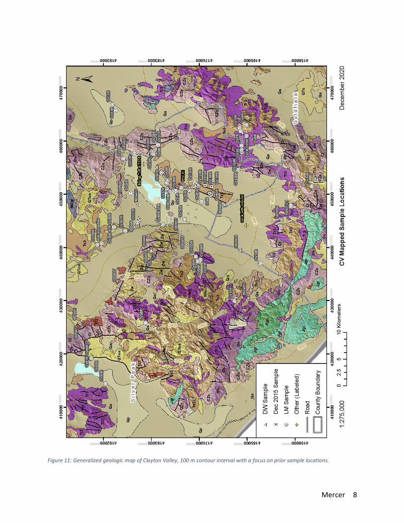
Figure 11 features this same map with a 100 m contour interval for clarity. This serves the purpose of the map as we are able to more clearly see the previous sampling locations derived from my group’s KMZ file. Because Figure 11 can be viewed referencing either the Figure 10 generalized geologic map or the Figure 12 explanation, geologic units were not included in the legend.

Figure 13 features the georeferenced surficial deposits map with sample locations layered on top. The NBMG geologic units were used below the image to provide more spatial reference.

Finally, Figure 14 uses USFWS wetland data and NDWR groundwater basin polygons to outline hydrologic features in the basin. There is a clear pattern to riverine flow when these features are placed over the hillshade. Sample locations were included on this map as well for referencing locations that might be important for geochemistry.

Mercer 7

Figure 10: Generalized geologic map of Clayton Valley, 50 m contour interval with no sample locations.

Mercer 8

Figure 11: Generalized geologic map of Clayton Valley, 100 m contour interval with a focus on prior sample locations.

Mercer 9

Figure 12: Explanation of geologic units in Figures 10, 11, and 13.

Mercer 10

Figure 13: Georeferenced surficial deposits in selected parts of Esmerelda County with sample locations overlain.

Mercer 11

Figure 14: Hydrologic map of Clayton Valley identifying watersheds and wetlands with sample locations.

Mercer 12

V. Conclusion The main goal of this project was to produce a comprehensive, well-organized folder that

could be shared among my teammates with a geodatabase established for field collection. Through the use of ArcCatalog, online resources, georeferencing, raster tools, and geoprocessing tools, four maps were created overlain with previously recorded field data previously unused in a KMZ file. Moving forward, the file geodatabase I created will be able to be uploaded to ArcGIS Online when needed for field work in May. Not only will the use of editable layers and domains expedite our field work, but the visualization of previous samples on geologic and hydrologic maps will allow us to easily plan sampling locations prior to travel. The maps created in this report can be packaged to ensure that the transfer of MXDs between team members would be seamless.