stepwise ctl model checking of state/event systems · stepwise ctl model checking of state/event...

Stepwise CTL Model Checking ofState/Event Systems

Jørn Lind-Nielsen and Henrik Reif Andersen

Department of Information Technology, Technical University of Denmarke-mail: {jl,hra}@it.dtu.dk

Abstract. In this paper we present an efficient technique for symbolicmodel checking of any CTL formula with respect to a state/event system.Such a system is a concurrent version of a Mealy machine and is usedto describe embedded reactive systems. The technique uses compositio-nality to find increasingly better upper and lower bounds of the solutionto a CTL formula until an exact answer is found. Experiments showthis approach to succeed on examples larger than the standard back-wards traversal can handle, and even in many cases where both methodssucceed it is shown to be faster.

1 Introduction

The range of systems that can be formally verified has improved drasticallysince the introduction of symbolic model checking [7,8] with the use of reducedand ordered binary decision diagrams (ROBDD) in the eighties [3,2]. Since thenmany people have improved on the basic algorithms by introducing more efficienttechniques, more compact representations and new methods for simplifying themodels.

One way to do simplifications on the model is by abstraction, where sub-components of the system considered are removed to yield a smaller and simplermodel on which the verification can be done. The technique described here isbased on one such incremental abstraction of the system, where first an initiallysmall subset of the system is used as an abstraction. If this set is not enough toprove or disprove the requirements then the set is incrementally extended untila point where it is possible to give an exact positive or negative answer.

The experimental results are promising and show that the iterative approachcan be used with success on larger systems than the usual backwards traversalcan handle, and it is still faster even when the usual method is feasible.

This work is a direct extension of the work presented at TACAS’98 [11]. Nowthe technique covers full CTL model checking and calculates simultaneously bothan upper and a lower approximation to the solution of the CTL formula.

We apply this technique to the state/event model used in the commercialtool visualSTATEtm [13]. This model is a concurrent version of Mealy machines,that is, it consists of a fixed number of concurrent finite state machines thathave pairs of input events and output actions associated with the transitions of

N. Halbwachs and D. Peled (Eds.): CAV’99, LNCS 1633, pp. 316–327, 1999.c© Springer-Verlag Berlin Heidelberg 1999

Stepwise CTL Model Checking of State/Event Systems 317

the machines. The model is synchronous: each input event is reacted upon byall machines in lock-step; the total output is the multi-set union of the outputactions of the individual machines. Further synchronization between the machi-nes is achieved by associating a guard with the transitions. Guards are Booleancombinations of conditions on the local states of the other machines.

Both the state space and the transition relation of the state/event systemis represented using ROBDDs with a partitioned transition relation, exactly asdescribed in [11].

1.1 Related Work

Another similar technique for exploiting the structure of the system to be verifiedis described in [9]. This technique also computes increasingly better approxima-tions to the exact solution of a CTL formula, but it differs from our approachin several ways. Instead of reusing the previously found states as shown in sec-tion 6, this technique has to recalculate the approximation from scratch eachtime a new component is added to the system. It may also have to include allcomponents in the system, whereas we restrict our inclusion to only the depen-dency closure (cone of influence) of the formula used. Finally the technique isrestricted to ACTL(ECTL) formulae, whereas our technique can be used withany CTL formula.

Pardo and Hachtel describes an abstraction technique in [14] where the ap-proximations are done using ROBDD reduction techniques. This technique isbased on the µ-calculus (and so includes CTL). It utilizes the structure of agiven formula to find appropriate abstractions, whereas our technique dependson the structure of the model.

The technique for showing language containment of L-processes describedin [1], also maintains a subset of processes used in the verification and analyzeserror traces from the verifier to find new processes in order to extend this set.Although the overall goal of finding the result through an abstract, simplifiedmodel is the same as our, the properties verified are different and the L-processeshave properties quite different from ours.

Abstraction as in [5] is similar to ours when the full dependency closureis included from the beginning, and thus it discards the idea of an iterativeapproach.

The idea of abstraction and compositionality is explored in more detail inDavid Longs’ thesis [12].

2 State/Event Systems

A state/event system S consists of n machines M1, . . . , Mn, an alphabet Eof input events and an alphabet O of outputs. Each machine Mi is a triple(Si, s0

i , Ti) of local states Si, an initial state s0i ∈ Si, and a set of transitions Ti.

The set of transitions is a relation

Ti ⊆ Si × E × Gi × M(O) × Si,

318 J. Lind-Nielsen and H.R. Andersen

e2

e1p1p0

M1

l2 = q1

e2

e1q1q0

M2

p0, q0 p1, q0

p1, q1p0, q1

e2

e1

e2

e1

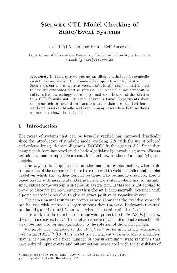
Fig. 1. Two state/event machines and the corresponding parallel combination. Thesmall arrows indicate the initial states.

where M(O) is a multi-set of outputs, and Gi is the set of guards not containingreferences to machine i. These guards are generated from the following simplegrammar for Boolean expressions:

g ::= lj = p | ¬g | g ∧ g | tt .

The atomic predicate lj = p is read as “machine j is at local state p” andtt denotes a true guard. The global state set S of the state/event system is theproduct of the local state sets: S = S1 ×S2 ×· · ·×Sn. The guards are interpretedstraightforwardly over S as given by a satisfaction relation s |= g. The expressionlj = p holds for any s ∈ S exactly when the j’th component of s is p, i.e., sj = p.The interpretation of the other cases is as usual. The transition relation is total,by assuming that the system stays in its current state when no transitions areenabled for a given input event.

Considering a global state s, all guards in the transition relation can beevaluated. We define a version of the transition relation in which the guardshave been evaluated. This relation is denoted s

e o−−→i s′i expressing that machine

i when receiving input event e makes a transition from si to s′i and generates

output o (here si is the i’th component of s). Formally,

se o−−→i s′

i ⇔def ∃g. (si, e, g, o, s′i) ∈ Ti and s |= g .

The transition relation of the whole system is defined as:

se o−−→ s′ ⇔def ∀i. s

e oi−−→i s′i where s′ = (s′

1, . . . , s′n) and o = o1 ] . . . ] on

Where ] denotes multi set union. The example in figure 1 shows a system withtwo state/event machines and the corresponding parallel combination. MachineM2 starts in state q0 and goes to state q1 on the receipt of event e1. Machine M1can not move on e1 because of the guard. After this M2 may go back on evente2 or M1 may enter state p1 on event e1. At last both M1 and M2 can return totheir initial states on event e2.

3 CTL Specifications

CTL [6] is a temporal logic used to specify formal requirements to finite statemachines like the state/event systems presented here. Such specifications consist


of the Boolean constant true tt, conjunction ∧, negation ¬, state predicates andtemporal operators. We use a state predicate variant where the location of amachine is stated: li = s meaning that machine i should be in state s, similar tothe guards.

The temporal operators are the next operator X(φ), the future operator F(φ),the globally operator G(φ) and the until operator (φ1U φ2). Each of these ope-rators must be directly preceded with a path quantifier to state whether theformula should hold for all possible execution paths of the system (A) or onlyfor at least one execution path (E).

The solution to a CTL formula φ is the set of states [[φ]] that satisfy theformula φ. A state/event system S is said to satisfy the property φ, S |= φ if theinitial state s0 is in the solution to φ, s0 ∈ [[φ]].

To describe the exact semantics of the operators we use an additional function[[EX]] that operates on a set of states P . This function returns all the states thatmay reach at least one of the states in P in exactly one step and is defined as[[EX]] P = {s ∈ S | ∃e, o, s′. s

e o−−→ s′ ∧ s′ ∈ P}. The operators are then defined,for a State/Event system with the transition relation s

e o−−→ s′, as:

[[tt]] = S [[li = s]] = {s′ ∈ S | s′i = s}

[[¬φ]] = S\[[φ]] [[φ1 ∧ φ2]] = [[φ1]] ∩ [[φ2]][[EX φ]] = [[EX]][[φ]] [[EG φ]] = νU ⊆ S. [[φ]] ∩ [[EX]]U

[[E(φ1 U φ2)]] = µU ⊆ S. [[φ2]] ∪ ([[φ1]] ∩ [[EX]]U)

Here we use νx.f(x) and µx.f(x) as the maximal and minimal fixed points of amonotone function f on a complete lattice, as given by Tarski’s fixed point theo-rem [16]. The rest of the operators can be defined using the above operators [8].

4 Bounded CTL Solutions

In this section we introduce the bounded CTL solution. A bounded CTL solutionconsists of two sets of states, namely L[[φ]]I and U [[φ]]I which are lower- and upperapproximations to the solution of the formula. The idea is to test for inclusionof the initial state in L[[φ]]I and exclusion from U [[φ]]I . In the first case we knowthat the formula holds and in the second that it does not.

To describe bounded CTL solutions we need to formalize the concept ofdependency between machines in a state/event system. We choose the notionthat one machine Mi depends on another machine Mj if there exists at least oneguard in Mi that has a syntactic reference to a state in Mj . These dependenciesform a directed graph, which we call the dependency graph. In this graph eachvertex represent a machine and an edge from a vertex i to a vertex j representsa dependency in machine Mi on a state in machine Mj . Note that we can ignoreany dependencies introduced by the global synchronization of the input events.

A formula φ depends on a machine Mi if φ contains a sub-formula of theform li = s, and the sort of φ is all the machines φ depends on. The dependencyclosure of a machine Mi is all the machines that are reachable from Mi in the


dependency graph, including Mi. This is also sometimes refered to as the coneof influence. The dependency closure of a formula φ is the union of all thedependency closures of the machines in the sort of φ.

Assume (for the time being) that we have an efficient way to calculate abounded solution to a CTL formula φ using only the machines in an index setI. The result should be two sets of states L[[φ]]I and U [[φ]]I with the followingproperties:

L[[φ]]I ⊆ [[φ]] ⊆ U [[φ]]I . (1)L[[φ]]I1 ⊆ L[[φ]]I2 if I1 ⊆ I2. (2)U [[φ]]I1 ⊇ U [[φ]]I2 if I1 ⊆ I2. (3)L[[φ]]I = [[φ]] = U [[φ]]I if I is dependency closed. (4)

Both L[[φ]]I and U [[φ]]I are only defined for sets I that include the sort of φ.Property (1) means that L[[φ]]I is a lower approximation of [[φ]] and U [[φ]]I is anupper approximation of [[φ]]. Property (2) and (3) mean that the approximationsconverge monotonically towards the correct solution of φ and property (4) statesthat we get the correct solution to φ when I contains all the machines found inthe dependency closure of φ.

In section 5 we will show an algorithm that efficiently computes the boundedsolution to any CTL formulae. With this, it is possible to make a serious impro-vement to the usual algorithm for finding CTL solutions. The algorithm utilizesthe fact that we may be able to prove or disprove the property φ using only a(hopefully) small subset of all the machines in the system.

Our algorithm for verifying a CTL property is as follows

Algorithm CTL verifierInput: A CTL formula φ and a state/event system S and it’s depen-

dency graph GOutput: true if s0 ∈ [[φ]] and false otherwise1. I = sort(φ); result = unknown2. repeat3. calculate L[[φ]]I and U [[φ]]I4. if s0 ∈ L[[φ]]I then result = true5. if s0 6∈ U [[φ]]I then result = false6. I = I ∪ extend(I, G)7. until result 6= unknown

First we set I to be the sort of φ and use this to calculate L[[φ]]I and U [[φ]]I . Ifs0 ∈ L[[φ]]I , then we know, from property (2), that φ holds for the system, and ifs0 6∈ U [[φ]]I then we know, from property (3), that φ does not hold. If neither isthe case then we add more machines to I and try again. This continues until φis either proved or disproved. The algorithm is guaranteed to stop with either afalse or a true result when I is the dependency closure of φ, in which case we haveL[[φ]]I = U [[φ]]I , from property (4), and thus either s0 ∈ L[[φ]]I or s0 6∈ U [[φ]]I .


The function extend selects a new set of machines to be included in I. Wehave chosen to include new machines in a breadth-first manner, so that extendreturns all machines reachable in G from I in one step.

5 Bounded CTL Calculation

In section 4 we showed how to verify a CTL formula φ, by using only a minimalset of machines I from a state/event system and using an efficient algorithm forthe calculation of lower and upper approximations of [[φ]]. In this section we willshow one such algorithm, and for this we need some more definitions. Relatingto an index set I of machines, two states s, s′ ∈ S are I-equivalent, written ass =I s′, if for all i ∈ I, si = s′

i. A set of states P is I-sorted if the followingpredicate is true

I-sorted(P ) ⇔def ∀s, s′ ∈ S. (s ∈ P ∧ s =I s′) ⇒ s′ ∈ P.

This means that if a state s is in P then all other states s′, which are I-equivalentto s, must also be in the set P . This is equivalent to say that a set P is I-sortedif it is independent of the machines in the complement I = {1, . . . , n} \ I.

Consider as an example two machines with the sets of states S0 = {p0, p1},S1 = {q0, q1, q2} and a sort I = {0}. Now the two pairs of states (p0, q1)and (p0, q2) are I-equivalent because their first states match. The set P ={(p0, q0), (p0, q1), (p0, q2)} is I-sorted because it is independent of the states inS1.

The bounded calculation of the constants tt and li = s, negation and con-junction is straight forward as shown in figure 2. The results are clearly I-sortedand satisfies the properties in section 4, if the sub-expressions φ, φ1 and φ2 doesso.

Next State Operator: To show how to find L[[EX φ]]I and U [[EX φ]]I weintroduce two new operators: [[E∀X]]I and [[E∃X]]I . The lower approximation[[E∀X]]I P is a conservative approximation to [[EX]] that only includes states thatare guaranteed to reach P in one step, regardless of the states of the machinesin I. The upper approximation [[E∃X]]I P is an optimistic approximation thatincludes all states that just might reach P . These two operators are defined as:

[[E∀X]]I P = {s ∈ S | ∀s′ ∈ S. s =I s′ ⇒ s′ ∈ [[EX]]I P}[[E∃X]]I P = {s ∈ S | ∃s′ ∈ S. s =I s′ ∧ s′ ∈ [[EX]]I P}

where the results of both operators are I-sorted when [[EX]]I P is I-sorted, as aresult of the extra quantifiers. The calculation of [[EX]]I P can be done efficientlywhen P is I-sorted, using a partitioned transition relation [4]. The definition of[[EX]]I is

[[EX]]I P = {s ∈ S | ∃e, o, s′. se o−−→ s′ ∧ s′ ∈ P}.


This seems to depend on all n machines in S, but as a result of P being I-sorted,it can be reduced to

[[EX]]I P = {s ∈ S | ∃e, o. ∃s′I. ∃s′

I . se o−−→I s′

I ∧ (s′1, . . . , s′

N ) ∈ P}

where ∃s′I . s

e o−−→I s′I means

∧i∈I ∃s′

i. se o−−→i s′

i. This clearly depends on onlythe transition relations for the machines in I.

Now we can define L[[EX φ]]I and U [[EX φ]]I as

L[[EX φ]]I = [[E∀X]]I L[[φ]]IU [[EX φ]]I = [[E∃X]]I U [[φ]]I .

Both L[[EX φ]]I and U [[EX φ]]I are clearly I-sorted because both [[E∀X]]I and[[E∃X]]I are so, and if φ satisfies the properties in section 4 then so does L[[EX φ]]Iand U [[EX φ]]I .

Globally and Until operators: The semantics for EG φ is defined in thesame manner as EX φ, with an added fixed point calculation:

L[[EG φ]]I = νU. L[[φ]]I ∩ [[E∀X]]IUU [[EG φ]]I = νU. U [[φ]]I ∩ [[E∃X]]IU.

The result is also I-sorted and satisfies the properties in section 4 if φ does. ForE(φ1 U φ2) we take

L[[E(φ1 U φ2)]]I = µU. L[[φ2]]I ∪ (L[[φ1]]I ∩ [[E∀X]]I U)U [[E(φ1 U φ2)]]I = µU. U [[φ2]]I ∪ (U [[φ1]]I ∩ [[E∃X]]I U).

6 Reusing Bounded CTL Calculations

One problem with the operators L[[φ]]I and U [[φ]]I from section 5, when usedin the bounded CTL verifier, is that all previously found states have to berediscovered whenever a new set of machines I is introduced. In this sectionwe will show how to avoid this problem for the EG operator and sketch how todo it for the E(φ1U φ2) operator. The final algorithm is shown in figure 2.

First we show how the calculation of U [[EG φ]]I2 can be improved by reusingthe previous calculation of U [[EG φ]]I1 when I1 ⊆ I2. From the definition ofU [[EG φ]]I we get the following:

U [[EG φ]]I2 ⊆ U [[EG φ]]I1 ⊆ U [[φ]]I1 andU [[EG φ]]I2 ⊆ U [[φ]]I2 ⊆ U [[φ]]I1

and from this we know that

U [[EG φ]]I2 ⊆ U [[EG φ]]I1 ∩ U [[φ]]I2 .

We also know, from Tarski’s fixed point theorem, that νf ⊆ x ⇒ νf =⋂i f

i(x),which means the maximum fixed point calculation of f can be started from any


B[[tt]]Ik = (S , S)

B[[li = s]]Ik = let L = {s′ ∈ S | s′i = s}

U = {s′ ∈ S | s′i = s}

in (L, U)

B[[¬φ]]Ik = let (L, U) = B[[φ]]Ikin (S \ U , S \ L)

B[[φ1 ∧ φ2]]Ik = let (L1, U1) = B[[φ1]]Ik(L2, U2) = B[[φ2]]Ik

in (L1 ∩ L2 , U1 ∩ U2)

B[[EX φ]]Ik = let (L, U) = B[[φ]]Ikin ([[E∀X]]Ik L , [[E∃X]]Ik U)

B[[EG φ]]Ik = let (L1, U1) = B[[φ]]Ik( , U2) = B[[EG φ]]Ik−1

U = νV. (U1 ∩ U2) ∩ [[E∃X]]IkV (a)L = νV. (L1 ∩ U) ∩ [[E∀X]]IkV (b)

in (L , U)

B[[E (φ1U φ2)]]Ik = let (L1, U1) = B[[φ1]]Ik(L2, U2) = B[[φ2]]Ik(L3, ) = B[[E (φ1U φ2)]]Ik−1

L = µV. (L2 ∪ L3) ∪ (L1 ∩ [[E∃X]]IkV ) (c)U = µV. (U2 ∪ L) ∪ (U1 ∩ [[E∃X]]IkV ) (d)

in (L , U)

Fig. 2. Full description of how the lower and upper approximations (L[[φ]]I , U [[φ]]I) =B[[φ]]I are calculated for a state/event system S. The sorts are Ik for the current sortand Ik−1 for the previous sort. Initially we have B[[φ]]I0 = (∅, S) and I0 is the sort ofthe expression. We use L for a lower approximation and U for an upper approximation.The lines (a)–(d) show where we reuse previously found states.

x as long as x includes the maximal fixed point of f . Here we use f i(x) as thei’th application of f on itself. From this it is clear that the fixed point calculationof U [[EG φ]]I2 can be started from the intersection of the two sets U [[EG φ]]I1and U [[φ]]I2 . Normally this fixed point calculation would have been started fromU [[φ]]I2 , but in this way we reuse the calculation of U [[EG φ]]I1 to speed up thecalculation of U [[EG φ]]I2 .

The same idea can be used for the lower approximation L[[EG φ]]I2 , wherethe fixed point iteration can be started from the intersection of L[[φ]]I2 andU [[EG φ]]I2 , so that we reuse the calculation of the upper approximation. Thealgorithm in figure 2 utilizes this in line (a) for the upper approximation and inline (b) for the lower approximation.

Exactly the same can be done for L[[E(φ1U φ2)]]I and U [[E(φ1U φ2)]]I , exceptthat the previous lower approximations should be used to restart the calculation,as shown in line c and d in figure 2.


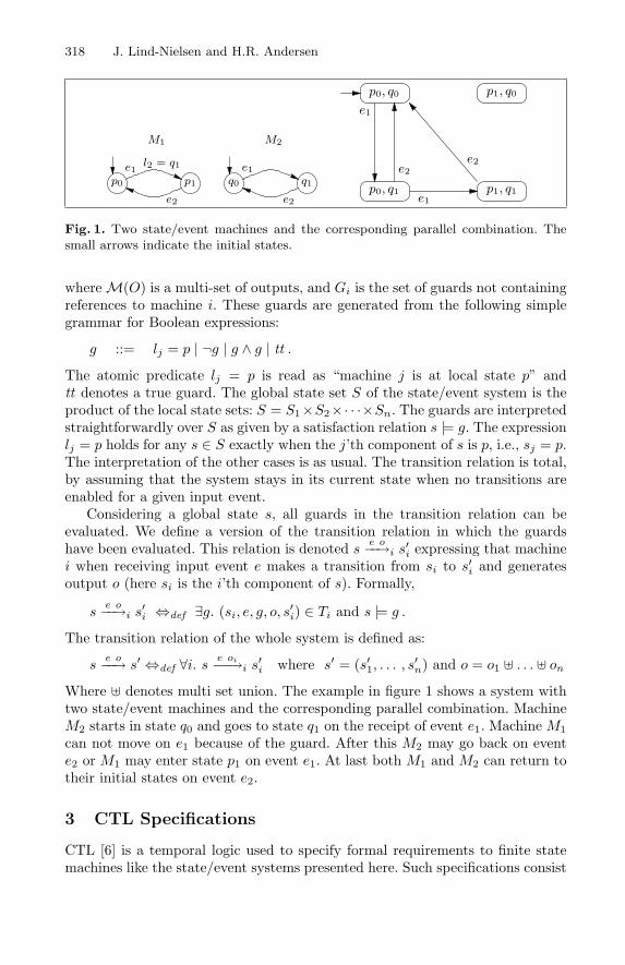
System Machines Local states Declared Reachableintervm 6 182 106 15144vcr 7 46 105 1279dkvm 9 55 106 377568hi-fi 9 59 107 1416384flow 10 232 105 17040motor 12 41 106 34560avs 12 66 107 1438416video 13 74 108 1219440atc 14 194 1010 6399552oil 24 96 1013 237230192train1 373 931 10136 −train2 1421 3204 10476 −

Table 1. The state/event systems used in the experiments. The last two columnsshow the size of the declared and reachable state space. The size of the declared statespace is the product of the number of local states of each machine. The reachable statespace is only known for those systems where a forward iteration of the state space cancomplete.

7 Examples

The technique presented here has been tested on ten industrial state/event sy-stems and two systems constructed by students in a course on embedded systems.The examples are all constructed using visualSTATEtm [13] and cover a largerange of different applications. The examples are hi-fi, avs, atc, flow, mo-tor, intervm, dkvm, oil, train1 and train2 which are industrial examplesand vcr and video which are constructed by students. In table 1 we have listedsome characteristics for these examples.

The experiments were carried out on a pentium 166MHz PC with 32Mb ofmemory, running Linux. For the ROBDD encoding we used BuDDy [10], a locallyproduced ROBDD package which is comparable in efficiency to other state ofthe art ROBDD packages, such as CUDD [15].

For each example we tested three different sets of CTL formulae. One setof formulae for detecting non-determinism in the system, one set for detectinglocal deadlocks and one for finding homestates.

Non-determinism occurs when two transitions leading out of a state dependson the same event and has guards that are enabled at the same time in a reach-able global state. That is, the intersection of the two guards g = g1 ∧ g2 shouldbe non-empty and reachable. Every combination of guards were then checkedfor reachability using the formula EF g.

Locally deadlocked states are local states from which there can never beenabled any outgoing transition, no matter how the rest of the system behaves.So for each local state s in the system we check for absence of local deadlocksusing the formula AG (s ⇒ EF ¬s)


Homestates are states that can be reached from any point in the reachablestate space. So for each local state s of the system we get the formula AG (EF s).

We have unfortunately only access to the examples in an anonymous form,so we have no way of generating more specialized properties.

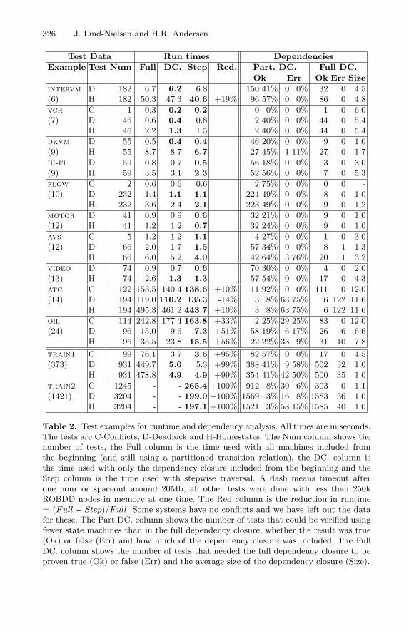
In table 2 we have listed the time it takes to complete checking a whole set ofCTL formulae using the standard backwards traversal with either all machinesin the system or only the machines in the dependency closure, and the time usedwith stepwise traversal. For the largest system it is only the stepwise traversalthat succeeds and with the exception of one system (atc) the stepwise traversalis also faster or comparable in speed to the standard backwards traversal.

We have also shown the number of tests that can be verified using fewermachines than in the dependency closure, how much of the dependency closurethere was needed to do it, how many tests that had to include the full depen-dency closure and the average size of that dependency closure. From this wecan see that in the train2 example we can verify most of the formulae usingonly a small fraction (3 − 15%) of the dependency closure and when the fulldependency closure has to be included then the average size of it is only as littleas 1 ( although we know that some tests includes more than 200 machines in thedependency closure). This indicates that train2 is a loosely coupled system i.e.a system with few dependencies among the state machines.

We also see that atc and oil are more strongly coupled, as the averagedependency closure is larger than for the other examples. This property is alsomirrored in the time needed to verify the two examples.

8 Conclusion

We have extended the successful model checking technique presented in [11]with the ability to do full CTL model checking and not only reachability anddeadlock detection. We have also added the calculation of both upper and lowerapproximations to the result and in this way making it possible to stop earlierin the verification process with either a negative or a positive answer.

Test examples have shown the stepwise traversal of the state space to bemore efficient, than the normal backwards traversal, in terms of both time andspace for a range of industrial examples. We have also shown that the stepwisetechnique may succeed in cases where the standard techniques fails.

The examples also indicates that the stepwise traversal works best on looselycoupled systems, that is; systems with few dependencies among the involvedstate machines.

Acknowledgement

Thanks to the colleagues of the VVS project for numerous fruitful discussionson the verification of state/event models.


Test Data Run times DependenciesExample Test Num Full DC. Step Red. Part. DC. Full DC.

Ok Err Ok Err Sizeintervm D 182 6.7 6.2 6.8 150 41% 0 0% 32 0 4.5(6) H 182 50.3 47.3 40.6 +19% 96 57% 0 0% 86 0 4.8vcr C 1 0.3 0.2 0.2 0 0% 0 0% 1 0 6.0(7) D 46 0.6 0.4 0.8 2 40% 0 0% 44 0 5.4

H 46 2.2 1.3 1.5 2 40% 0 0% 44 0 5.4dkvm D 55 0.5 0.4 0.4 46 20% 0 0% 9 0 1.0(9) H 55 8.7 8.7 6.7 27 45% 1 11% 27 0 1.7hi-fi D 59 0.8 0.7 0.5 56 18% 0 0% 3 0 3.0(9) H 59 3.5 3.1 2.3 52 56% 0 0% 7 0 5.3flow C 2 0.6 0.6 0.6 2 75% 0 0% 0 0 -(10) D 232 1.4 1.1 1.1 224 49% 0 0% 8 0 1.0

H 232 3.6 2.4 2.1 223 49% 0 0% 9 0 1.2motor D 41 0.9 0.9 0.6 32 21% 0 0% 9 0 1.0(12) H 41 1.2 1.2 0.7 32 24% 0 0% 9 0 1.0avs C 5 1.2 1.2 1.1 4 27% 0 0% 1 0 3.0(12) D 66 2.0 1.7 1.5 57 34% 0 0% 8 1 1.3

H 66 6.0 5.2 4.0 42 64% 3 76% 20 1 3.2video D 74 0.9 0.7 0.6 70 30% 0 0% 4 0 2.0(13) H 74 2.6 1.3 1.3 57 54% 0 0% 17 0 4.3atc C 122 153.5 140.4 138.6 +10% 11 92% 0 0% 111 0 12.0(14) D 194 119.0 110.2 135.3 -14% 3 8% 63 75% 6 122 11.6

H 194 495.3 461.2 443.7 +10% 3 8% 63 75% 6 122 11.6oil C 114 242.8 177.4 163.8 +33% 2 25% 29 25% 83 0 12.0(24) D 96 15.0 9.6 7.3 +51% 58 19% 6 17% 26 6 6.6

H 96 35.5 23.8 15.5 +56% 22 22% 33 9% 31 10 7.8train1 C 99 76.1 3.7 3.6 +95% 82 57% 0 0% 17 0 4.5(373) D 931 449.7 5.0 5.3 +99% 388 41% 9 58% 502 32 1.0

H 931 478.8 4.9 4.9 +99% 354 41% 42 50% 500 35 1.0train2 C 1245 - - 265.4 +100% 912 8% 30 6% 303 0 1.1(1421) D 3204 - - 199.0 +100% 1569 3% 16 8% 1583 36 1.0

H 3204 - - 197.1 +100% 1521 3% 58 15% 1585 40 1.0

Table 2. Test examples for runtime and dependency analysis. All times are in seconds.The tests are C-Conflicts, D-Deadlock and H-Homestates. The Num column shows thenumber of tests, the Full column is the time used with all machines included fromthe beginning (and still using a partitioned transition relation), the DC. column isthe time used with only the dependency closure included from the beginning and theStep column is the time used with stepwise traversal. A dash means timeout afterone hour or spaceout around 20Mb, all other tests were done with less than 250kROBDD nodes in memory at one time. The Red column is the reduction in runtime= (Full − Step)/Full. Some systems have no conflicts and we have left out the datafor these. The Part.DC. column shows the number of tests that could be verified usingfewer state machines than in the full dependency closure, whether the result was true(Ok) or false (Err) and how much of the dependency closure was included. The FullDC. column shows the number of tests that needed the full dependency closure to beproven true (Ok) or false (Err) and the average size of the dependency closure (Size).


References

1. F. Balarin and A.L. Sangiovanni-Vincentelli. An iterative approach to languagecontainment. In C. Courcoubetis, editor, CAV’93. 5th International Conferenceon Computer Aided Verification, volume 697 of LNCS, pages 29–40, Berlin, 1993.Springer-Verlag.

2. Randal E. Bryant. Graph-Based Algorithms for Boolean Function Manipulation.IEEE Transactions on Computers, C-35(8):677–691, August 1986.

3. Randal E. Bryant. Symbolic Boolean manipulation with ordered binary decisiondiagrams. ACM Computing Surveys, 24(3):293–318, September 1992.

4. J. R. Burch, E. M. Clarke, and D. E. Long. Symbolic model checking with parti-tioned transition relations. In A. Halaas and P. B. Denyer, editors, Proc. 1991 Int.Conf. on VLSI, August 1991.

5. William Chan, Richard J. Anderson, Paul Beame, and David Notkin. Improvingefficiency of symbolic model checking for state-based system requirements. InProceedings of the ACM SIGSOFT International Symposium on Software Testingand Analysis (ISSTA-98), volume 23,2 of ACM Software Engineering Notes, pages102–112, New York, March2–5 1998. ACM Press.

6. E. M. Clarke, E. A. Emerson, and A. P. Sistla. Automatic verification of finite-state concurrent systems using temporal logic specifications. ACM Transactionson Programming Languages and Systems, 8(2):244–263, April 1986.

7. J.R. Burch, E.M. Clarke, D.E. Long, K.L. MacMillan, and D.L. Dill. Symbolicmodel checking for sequential circuit verification. IEEE Transactions on Computer-Aided Design of Integrated Circuits and Systems, 13(4):401–424, April 1994.

8. J.R. Burch, E.M. Clarke, K.L. McMillan, and D.L. Dill. Sequential Circuit Veri-fication Using Symbolic Model Checking. In Proceedings of the 27th ACM/IEEEDesign Automation Conference, pages 46–51, Los Alamitos, CA, June 1990.ACM/IEEE, IEEE Society Press.

9. W. Lee, A. Pardo, J.-Y. Jang, G. Hachtel, and F. Somenzi. Tearing based au-tomatic abstraction for CTL model checking. In Proceedings of the IEEE/ACMInternational Conference on Computer-Aided Design, pages 76–81, Washington,November10–14 1996. IEEE Computer Society Press.

10. Jørn Lind-Nielsen. BuDDy - A Binary Decision Diagram Package. TechnicalUniversity of Denmark, 1997. http://britta.it.dtu.dk/˜jl/buddy.

11. Jørn Lind-Nielsen, Henrik Reif Andersen, Gerd Behrmann, Henrik Hulgaard, K̊areKristoffersen, and Kim G. Larsen. Verification of Large State/Event Systems usingCompositionality and Dependency Analysis. In TACAS’98 Tools and Algorithmsfor the Construction and Analysis of Systems. Lecture Notes in Computer Science,1998.

12. David E. Long. Model Checking, Abstraction and Compositional Verification. PhDthesis, Carnegie Mellon, 1993.

13. Beologicr A/S. visualSTATEtm 3.0 User’s Guide, 1996.14. Abelardo Pardo and Gary D. Hachtel. Automatic abstraction techniques for pro-

positional µ-calculus model checking. In Computer Aided Verification, CAV’97.Springer Verlag, 1997.

15. Fabio Somenzi. CUDD: CU Decision Diagram Package. University of Colorado atBoulder, 1997.

16. A. Tarski. A lattice-theoretical fixpoint theorem and its application. PacificJ.Math., 5:285–309, 1955.

stepwise ctl model checking of state/event systems · stepwise ctl model checking of state/event...

Documents